Generalizing Distance Covariance to Measure

and Test Multivariate Mutual Dependence

Ze Jin, David S. Matteson∗

February 27, 2018

Abstract

We propose three new measures of mutual dependence between multiple random

vectors. Each measure is zero if and only if the random vectors are mutually indepen-

dent. The first generalizes distance covariance from pairwise dependence to mutual de-

pendence, while the other two measures are sums of squared distance covariances. The

proposed measures share similar properties and asymptotic distributions with distance

covariance, and capture non-linear and non-monotone mutual dependence between the

random vectors. Inspired by complete and incomplete V-statistics, we define empirical

and simplified empirical measures as a trade-off between the complexity and statistical

power when testing mutual independence. The implementation of corresponding tests

is demonstrated by both simulation results and real data examples.

Key words: characteristic functions; distance covariance; multivariate analysis; mutual in-

dependence; V-statistics

∗Research support from an NSF Award (DMS-1455172), a Xerox PARC Faculty Research Award, andCornell University Atkinson Center for a Sustainable Future (AVF-2017).

1

arX

iv:1

709.

0253

2v5

[m

ath.

ST]

25

Feb

2018

1 Introduction

Let X = (X1, . . . , Xd) be a set of variables where each component Xj, j = 1, . . . , d is a

continuous random vector, and let X = {Xk = (Xk1 , . . . , X

kd ) : k = 1, . . . , n} be an i.i.d.

sample from FX , the joint distribution of X. We are interested in testing the hypothesis

H0 : X1, . . . , Xd are mutually independent, HA : X1, . . . , Xd are dependent,

which has many applications, including independent component analysis (Matteson and

Tsay, 2017), graphical models (Fan et al., 2015), naive Bayes classifiers (Tibshirani et al.,

2002), etc. This problem has been studied under different settings and assumptions, including

pairwise (d = 2) and mutual (d ≥ 2) independence, univariate (X1, . . . , Xd ∈ R1) and

multivariate (X1 ∈ Rp1 , . . . , Xd ∈ Rpd) components, and more. Specifically, we focus on the

general case that X1, . . . , Xd are not assumed jointly normal.

The most extensively studied case is pairwise independence with univariate components

(X1, X2 ∈ R1): Rank correlation is considered as a non-parametric counterpart to Pear-

son’s product-moment correlation (Pearson, 1895), including Kendall’s τ (Kendall, 1938),

Spearman’s ρ (Spearman, 1904), etc. Bergsma and Dassios (2014) proposed a test based on

an extension of Kendall’s τ , testing an equivalent condition to H0. Additionally, Hoeffding

(1948) proposed a non-parametric test based on marginal and joint distribution functions,

testing a necessary condition to investigate H0.

For pairwise independence with multivariate components (X1 ∈ Rp1 , X2 ∈ Rp2): Szekely

et al. (2007), Szekely and Rizzo (2009) proposed a test based on distance covariance with

fixed p1, p2 and n → ∞, testing an equivalent condition to H0. Further, Szekely and Rizzo

(2013a) proposed a t-test based on a modified distance covariance for the setting in which n

is finite and p1, p2 →∞, testing an equivalent condition to H0 as well.

For mutual independence with univariate components (X1, . . . , Xd ∈ R1): One natural

2

way to extend the pairwise rank correlation to multiple components is to collect the rank

correlations between all pairs of components, and examine the norm (L2,L∞) of this collec-

tion. Leung and Drton (2015) proposed a test based on the L2 norm with n, d → ∞, and

d/n → γ ∈ (0,∞), and Han and Liu (2014) proposed a test based on the L∞ norm with

n, d→∞, and d/n→ γ ∈ [0,∞]. Each are testing a necessary condition to H0, in general.

For mutual independence with multivariate components (X1 ∈ Rp1 , . . . , Xd ∈ Rpd): This

challenging scenario has not been well studied. Yao et al. (2016) proposed a test based on

distance covariance between all pairs of components with n, d → ∞, testing a necessary

condition to H0. Inspired by distance covariance in Szekely et al. (2007), we propose a new

test based on measures of mutual dependence with fixed d, p1, . . . , pd and n → ∞ in this

paper, testing an equivalent condition to H0. All computational complexities in this paper

make no reference to the dimensions d, p1, . . . , pd, as they are treated as constants.

Our measures of mutual dependence involve V-statistics, and are 0 if and only if mutual

independence holds. They belong to energy statistics (Szekely and Rizzo, 2013b), and share

many statistical properties with distance covariance. Besides, Pfister et al. (2016) proposed

d-variable Hilbert−Schmidt independence criterion (dHSIC) under the same setting, which

originates from HSIC (Gretton et al., 2005), and also is 0 if and only if mutual independence

holds. Although dHSIC involves V-statistics as well, they pursue kernel methods and over-

come the computation bottleneck by resampling and Gamma approximation, while we take

advantage of characteristic functions and resort to incomplete V-statistics.

The weakness of testing mutual independence by a necessary condition, all pairwise in-

dependencies motivates our work on measures of mutual dependence, which is demonstrated

by examples in section 5: If we directly test mutual independence based on the measures

of mutual dependence proposed in this paper, we successfully detect mutual dependence.

Alternatively, if we check all pairwise independencies based on distance covariance, we fail

to detect any pairwise dependence, and mistakenly conclude that mutual independence holds

3

probably because the mutual effect averages out when we narrow down to a pair.

The rest of this paper is organized as follows. In section 2, we give a brief overview of

distance covariance. In section 3, we generalize distance covariance to complete measure

of mutual dependence, with its properties and asymptotic distributions derived. In section

4, we propose asymmetric and symmetric measures of mutual dependence, defined as sums

of squared distance covariances. We present synthetic and real data analysis in section 5,

followed by simulation results in section 61. Finally, section 7 is the summary of our work.

All proofs have been moved to appendix.

The following notations will be used throughout this paper. Let (·, ·, . . . , ·) denote a

concatenation of (vector) components into a vector. Let t = (t1, . . . , td), t0 = (t01, . . . , t

0d), X =

(X1, . . . , Xd) ∈ Rp where tj, t0j , Xj ∈ Rpj , such that pj is the marginal dimension, j = 1, . . . , d,

and p =∑d

j=1 pj is the total dimension. The assumed “X” under H0 is denoted by X =

(X1, . . . , Xd), where XjD= Xj, j = 1, . . . , d, X1, . . . , Xd are mutually independent, and

X, X are independent. Let X ′, X ′′ be independent copies of X, i.e., X,X ′, X ′′i.i.d.∼ FX , and

X ′, X ′′ be independent copies of X, i.e., X, X ′, X ′′i.i.d.∼ FX . Let the weighted L2 norm ‖ · ‖w

of complex-valued function η(t) be defined by ‖η(t)‖2w =

∫Rp |η(t)|2w(t) dt where |η(t)|2 =

η(t)η(t), η(t) is the complex conjugate of η(t), and w(t) is any positive weight function for

which the integral exists.

Given the i.i.d. sample X from FX , let Xj = {Xkj : k = 1, . . . , n} denote the correspond-

ing i.i.d. sample from FXj, j = 1, . . . , d, such that X = {X1, . . . ,Xd}. Denote the joint

characteristic functions of X and X as φX(t) = E[ei〈t,X〉] and φX(t) =∏d

j=1 E[ei〈tj ,Xj〉], and

denote the empirical versions of φX(t) and φX(t) as φnX(t) = 1n

∑nk=1 e

i〈t,Xk〉 and φnX

(t) =∏dj=1( 1

n

∑nk=1 e

i〈tj ,Xkj 〉).

1An accompanying R package EDMeasure (Jin et al., 2018) is available on CRAN.

4

2 Distance Covariance

Szekely et al. (2007) proposed distance covariance to capture non-linear and non-monotone

pairwise dependence between two random vectors (X1 ∈ Rp1 , X2 ∈ Rp2).

X1, X2 are pairwise independent if and only if φX(t) = φX1(t1)φX2(t2), ∀t, which is

equivalent to∫Rp |φX(t)− φX(t)|2w(t) dt = 0, ∀w(t) > 0 if the integral exists. A class of the

weight functions w0(t,m) = (K(p1;m)K(p2;m)|t1|p1+m|t2|p2+m)−1 make the integral a finite

and meaningful quantity composed of m-th moments according to Lemma 1 in Szekely and

Rizzo (2005), where K(q,m) = 2πq/2Γ(1−m/2)m2mΓ((q+m)/2)

, and Γ is the gamma function.

The non-negative distance covariance V(X) is defined by V2(X) = ‖φX(t)− φX(t)‖2w0

=∫Rp |φX(t)− φX(t)|2w0(t) dt, where

w0(t) = (Kp1Kp2|t1|p1+1|t2|p2+1)−1, (1)

with m = 1 and Kq = K(q, 1), while any following result can be generalized to 0 < m < 2. If

E|X| <∞, then V(X) ∈ [0,∞), and V(X) = 0 if and only ifX1, X2 are pairwise independent.

The non-negative empirical distance covariance Vn(X) is defined by V2n(X) = ‖φnX(t) −

φnX

(t)‖2w0

=∫Rp |φnX(t) − φn

X(t)|2w0(t) dt. Calculating V2

n(X) via the symmetry of Euclidian

distances has the time complexity O(n2). Some asymptotic properties of Vn(X) are derived.

If E|X| < ∞, then (i) Vn(X)a.s.−→n→∞

V(X). (ii) Under H0, nV2n(X)

D−→n→∞

‖ζ(t)‖2w0

where

ζ(t) is a complex-valued Gaussian process with mean zero and covariance function R(t, t0) =

[φX1(t1−t01)−φX1(t1)φX1(t01)][φX2(t2−t02)−φX2(t2)φX2(t

02)]. (iii) Under HA, nV2

n(X)a.s.−→n→∞

∞.

3 Complete Measure of Mutual Dependence

Generalizing the idea of distance covariance, we propose complete measure of mutual depen-

dence to capture non-linear and non-monotone mutual dependence between multiple random

5

vectors (X1 ∈ Rp1 , . . . , Xd ∈ Rpd).

X1, . . . , Xd are mutually independent if and only if φX(t) = φX1(t1) . . . φXd(td) = φX(t),

∀t, which is equivalent to∫Rp |φX(t) − φX(t)|2w(t) dt = 0, ∀w(t) > 0 if the integral exists.

We put all components together instead of separating them, and choose the weight function

w1(t) = (Kp|t|p+1)−1. (2)

Definition 1. The complete measure of mutual dependence Q(X) is defined by

Q(X) = ‖φX(t)− φX(t)‖2w1

=

∫Rp

|φX(t)− φX(t)|2w1(t) dt.

We can show an equivalence to mutual independence based on Q(X) according to Lemma

1 in Szekely and Rizzo (2005).

Theorem 1. If E|X| < ∞, then Q(X) ∈ [0,∞), and Q(X) = 0 if and only if X1, . . . , Xd

are mutually independent. In addition, Q(X) has an interpretation as expectations

Q(X) = E|X − X ′|+ E|X ′ − X| − E|X −X ′| − E|X − X ′|.

It is straightforward to estimate Q(X) by replacing the characteristic functions with the

empirical characteristic functions from the sample.

Definition 2. The empirical complete measure of mutual dependence Qn(X) is defined by

Qn(X) = ‖φnX(t)− φnX

(t)‖2w1

=

∫Rp

|φnX(t)− φnX

(t)|2w1(t) dt.

6

Lemma 1. Qn(X) has an interpretation as complete V-statistics

Qn(X) =2

nd+1

n∑k,`1,...,`d=1

|Xk − (X`11 , . . . , X

`dd )|+ 1

n2

n∑k,`=1

|Xk −X`|

− 1

n2d

n∑k1,...,kd,`1,...,`d=1

|(Xk11 , . . . , X

kdd )− (X`1

1 , . . . , X`dd )|,

whose naive implementation has the time complexity O(n2d).

In view of the definition of distance covariance, it may seem natural to define the measure

using the weight function

w2(t) = (Kp1 . . . Kpd|t1|p1+1 . . . |td|pd+1)−1, (3)

which equals w0(t) when d = 2. Given the weight function w2(t), we can define the squared

distance covariance of mutual dependence U(X) = ‖φX(t) − φX(t)‖2w2

and its empirical

counterpart Un(X) = ‖φnX(t) − φnX

(t)‖2w2

, which equal V2(X) and V2n(X) when d = 2. The

naive implementation of Un(X) has the time complexity O(nd+1).

The reason to favor w1(t) instead of w2(t) is a trade-off between the moment condition

and time complexity. We often cannot afford the time complexity of Qn(X) or Un(X), and

have to simplify them through incomplete V-statistics. An incomplete V-statistic is obtained

by sampling the terms of a complete V-statistic, where the summation extends over only a

subset of the tuple of indices. To simplify by replacing complete V-statistics with incom-

plete V-statistics, Un(X) requires the additional d-th moment condition E|X1 . . . Xd| < ∞,

while Qn(X) does not require any other condition in addition to the first moment condition

E|X| <∞. Thus, we can reduce the complexity of Qn(X) to O(n2) with a weaker condition,

which makes Q(X) and Qn(X) from w1(t) a more general solution. Moreover, we define the

7

simplified empirical version of φX(t) as

φn?X

(t) =1

n

n∑k=1

ei∑d

j=1〈tj ,Xk+j−1j 〉 =

1

n

n∑k=1

ei〈t,(Xk1 ,...,X

k+d−1d )〉,

in order to substitute φnX

(t) for simplification, where Xn+kj is interpreted as Xk

j for k > 0.

Definition 3. The simplified empirical complete measure of mutual dependence Q?n(X) is

defined by

Q?n(X) = ‖φnX(t)− φn?X

(t)‖2w1

=

∫Rp

|φnX(t)− φn?X

(t)|2w1(t) dt.

Lemma 2. Q?n(X) has an interpretation as incomplete V-statistics

Q?n(X) =2

n2

n∑k,`=1

|Xk − (X`1, . . . , X

`+d−1d )|+ 1

n2

n∑k,`=1

|Xk −X`|

− 1

n2

n∑k,`=1

|(Xk1 , . . . , X

k+d−1d )− (X`

1, . . . , X`+d−1d )|,

whose naive implementation has the time complexity O(n2).

Using a similar derivation to Theorem 2 and 5 of Szekely et al. (2007), some asymptotic

distributions of Qn(X),Q?n(X) are obtained as follows.

Theorem 2. If E|X| <∞, then

Qn(X)a.s.−→n→∞

Q(X) and Q?n(X)a.s.−→n→∞

Q(X).

Theorem 3. If E|X| <∞, then under H0, we have

nQn(X)D−→

n→∞‖ζ(t)‖2

w1and nQ?n(X)

D−→n→∞

‖ζ?(t)‖2w1,

where ζ(t), ζ?(t) are complex-valued Gaussian processes with mean zero and covariance func-

8

tions

R(t, t0) =d∏j=1

φXj(tj − t0j) + (d− 1)

d∏j=1

φXj(tj)φXj

(t0j)−d∑j=1

φXj(tj − t0j)

∏`6=j

φX`(t`)φX`

(t0`),

R?(t, t0) = 2R(t, t0).

Under HA, we have

nQn(X)a.s.−→n→∞

∞ and nQ?n(X)a.s.−→n→∞

∞.

Therefore, a mutual independence test can be proposed based on the weak convergence

of nQn(X), nQ?n(X) in Theorem 3. Since the asymptotic distributions of nQn(X), nQ?n(X)

depend on FX , a permutation procedure is used to approximate them in practice.

4 Asymmetric and Symmetric Measures of Mutual De-

pendence

As an alternative, we now propose the asymmetric and symmetric measures of mutual de-

pendence to capture mutual dependence via aggregating pairwise dependencies.

The subset of components on the right of Xc is denoted by Xc+ = (Xc+1, . . . , Xd), with

tc+ = (tc+1, . . . , td), c = 0, 1, . . . , d − 1. The subset of components except Xc is denoted by

X−c = (X1, . . . , Xc−1, Xc+), with t−c = (t1, . . . , tc−1, tc+), c = 1, . . . , d− 1.

We denote pairwise independence by ⊥⊥. The collection of pairwise independencies im-

plied by mutual independence includes “one versus others on the right”

{X1⊥⊥X1+ , X2⊥⊥X2+ , . . . , Xd−1⊥⊥Xd}, (4)

9

“one versus all the others”

{X1⊥⊥X−1, X2⊥⊥X−2, . . . , Xd⊥⊥X−d}, (5)

and many others, e.g., (X1, X2)⊥⊥X2+ . In fact, the number of pairwise independencies re-

sulting from mutual independence is at least 2d−1 − 1, which grows exponentially with the

number of components d. Therefore, we cannot test mutual independence simply by checking

all pairwise independencies even with moderate d.

Fortunately, we have two options to test only a small subset of all pairwise independencies

to fulfill the task. The first one is that H0 holds if and only if (4) holds, which can be verified

via the sequential decomposition of distribution functions. This option is asymmetric and

not unique, having d! feasible subsets with respect to different orders of X1, . . . , Xd. The

second one is that H0 holds if and only if (5) holds, which can be verified via the stepwise

decomposition of distribution functions and the fact that Xj⊥⊥X−j implies Xj⊥⊥Xj+ . This

option is symmetric and unique, having only one feasible subset.

To shed light on why these two options are necessary and sufficient conditions to mu-

tual independence, we present the following inequality that the mutual dependence can be

bounded by a sum of several pairwise dependencies as

|φX(t)−d∏j=1

φXj(tj)| ≤

d−1∑c=1

|φ(Xc,Xc+ )((tc, tc+))− φXc(tc)φXc+(tc+)|2.

In consideration of these two options, we test a set of pairwise independencies in place

of mutual independence, where we use V2(X) to test pairwise independence.

Definition 4. The asymmetric and symmetric measures of mutual dependence R(X),S(X)

10

are defined by

R(X) =d−1∑c=1

V2((Xc, Xc+)) and S(X) =d∑c=1

V2((Xc, X−c)).

We can show an equivalence to mutual independence based on R(X),S(X) according to

Theorem 3 of Szekely et al. (2007).

Theorem 4. If E|X| <∞, then R(X),S(X) ∈ [0,∞), and R(X),S(X) = 0 if and only if

X1, . . . , Xd are mutually independent.

It is straightforward to estimate R(X),S(X) by replacing the characteristic functions

with the empirical characteristic functions from the sample.

Definition 5. The empirical asymmetric and symmetric measures of mutual dependence

Rn(X),Sn(X) are defined by

Rn(X) =d−1∑c=1

V2n((Xc,Xc+)) and Sn(X) =

d∑c=1

V2n((Xc,X−c)).

The implementations of Rn(X),Sn(X) have the time complexity O(n2). Using a simi-

lar derivation to Theorem 2 and 5 of Szekely et al. (2007), some asymptotic properties of

Rn(X),Sn(X) are obtained as follows.

Theorem 5. If E|X| <∞, then

Rn(X)a.s.−→n→∞

R(X) and Sn(X)a.s.−→n→∞

S(X).

Theorem 6. If E|X| <∞, then under H0, we have

nRn(X)D−→

n→∞

d−1∑j=1

‖ζRj ((tj, tj+))‖2w0

and nSn(X)D−→

n→∞

d∑j=1

‖ζSj ((tj, t−j))‖2w0,

11

where ζRj ((tj, tj+)), ζSj ((tj, t−j)) are complex-valued Gaussian processes corresponding to the

limiting distributions of nV2n((Xj,Xj+)), nV2

n((Xj,X−j)). Under HA, we have

nRn(X)a.s.−→n→∞

∞ and nSn(X)a.s.−→n→∞

∞.

It is surprising to find that V2n((Xc,Xc+)), c = 1, . . . , d − 1 are mutually independent

asymptotically, and V2n((Xc,X−c)), c = 1, . . . , d are mutually independent asymptotically as

well, which is a crucial discovery behind Theorem 6.

Alternatively, we can plug in Q(X) instead of V2(X) in Definition 4 and Qn(X) instead

of V2n(X) in Definition 5, and define the asymmetric and symmetric measures J (X), I(X) ac-

cordingly, which equalQ(X),Qn(X) when d = 2. The naive implementations of Jn(X), In(X)

have the time complexity O(n4). Similarly, we can replace Qn(X) with Q?n(X) to simplify

them, and define the simplified empirical asymmetric and symmetric measures J ?n (X), I?n(X),

reducing their complexities to O(n2) without any other condition except the first moment

condition E|X| < ∞. Through the same derivations, we can show that Jn(X),J ?n (X),

In(X), I?n(X) have similar convergences as Rn(X),Sn(X) in Theorem 5 and 6.

5 Illustrative Examples

We start with two examples comparing different methods to show the value of our mutual

independence tests. In practice, people usually check all pairwise dependencies to test mutual

independence, due to the lack of reliable and universal mutual independence tests. It is very

likely to miss the complicated mutual dependence structure, and make unsound decisions in

corresponding applications assuming that mutual independence holds.

12

5.1 Synthetic Data

We define a triplet of random vectors (X, Y, Z) on Rq×Rq×Rq, where X, Y ∼ N (0, Iq), W ∼

Exp(1/√

2), the first element of Z is Z1 = sign(X1Y1)W and the remaining q − 1 elements

are Z2:q ∼ N (0, Iq−1), and X, Y,W,Z2:q are mutually independent. Clearly, (X, Y, Z) is a

pairwise independent but mutually dependent triplet.

An i.i.d. sample of (X, Y, Z) is randomly generated with sample size n = 500 and di-

mension q = 5. On the one hand, we test the null hypothesis H0 : X, Y, Z are mutually

independent using proposed measures Rn,Sn,Q?n,J ?n , I?n. On the other hand, we test the

null hypotheses H(1)0 : X⊥⊥Y , H

(2)0 : Y⊥⊥Z, and H

(3)0 : X⊥⊥Z using distance covariance V2

n.

An adaptive permutation size B = 210 is used for all tests.

As expected, mutual dependence is successfully captured, as the p-values of mutual inde-

pendence tests are 0.0143 (Q?n), 0.0286 (J ?n ), 0 (I?n), 0.0381 (Rn) and 0 (Sn). Meanwhile, the

p-values of pairwise independence tests are 0.2905 (X, Y ), 0.2619 (Y, Z), and 0.3048 (X,Z).

According to the Bonferroni correction for multiple tests among all the pairs, the signifi-

cance level should be adjusted as α/3 for pairwise tests. As a result, no signal of pairwise

dependence is detected, and we cannot reject mutual independence.

5.2 Financial Data

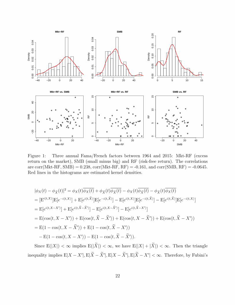
We collect the annual Fama/French 5 factors in the past 52 years between 1964 and 20152.

In particular, we are interested in whether mutual dependence among three factors, X =

Mkt-RF (excess return on the market), Y = SMB (small minus big), and Z = RF (risk-free

return) exists, where annual returns are considered as nearly independent observations. Both

histograms and pair plots of X, Y, Z are depicted in Figure 1.

For one, we apply a single mutual independence test H0 : X, Y, Z are mutually indepen-

2Data at http://mba.tuck.dartmouth.edu/pages/faculty/ken.french/data library.html.

13

dent. For another, we apply three pairwise independence tests H(1)0 : X⊥⊥Y , H

(2)0 : Y⊥⊥Z,

and H(3)0 : X⊥⊥Z. An adaptive permutation size B = 296 is used for all tests.

The p-values of mutual independence tests are 0.0236 (Q?n), 0.0642 (J ?n ), 0.0541 (I?n),

0.1588 (Rn) and 0.1486 (Sn), indicating that mutual dependence is successfully captured. In

the meanwhile, the p-values of pairwise independence tests using distance covariance V2n are

0.1419 (X, Y ), 0.5743 (Y, Z) and 0.5405 (X,Z). Similarly, the significance level should be

adjusted as α/3 according to the Bonferroni correction, and thus we cannot reject mutual

independence, since no signal of pairwise dependence is detected.

6 Simulation Studies

In this section, we evaluate the finite sample performance of proposed measures Qn,Rn,Sn,

Jn, In,Q?n,J ?n , I?n by performing simulations similar to Szekely et al. (2007), and compare

them to benchmark measures V2n (Szekely et al., 2007) and HLτ ,HLρ (Han and Liu, 2014).

We also include permutation tests based on finite-sample extensions of HLτ ,HLρ, denoted

by HLτn,HLρn.

We test the null hypothesis H0 with significance level α = 0.1 and examine the empirical

size and power of each measure. In each scenario, we run 1,000 repetitions with the adaptive

permutation size B = b200 + 5000/nc where n is the sample size, for all empirical measures

that require a permutation procedure to approximate their asymptotic distributions, i.e.,

Qn,Rn,Sn,Jn, In,Q?n,J ?n , I?n,V2

n.

In the following two examples, we fix d = 2 and change n from 25 to 500, and compare

Qn,Rn,Sn,Jn, In,Q?n,J ?n , I?n to V2

n.

Example 1 (pairwise multivariate normal). X1, X2 ∈ R5, (X1, X2)T ∼ N10(0,Σ) where

Σii = 1. Under H0, Σij = 0, i 6= j. Under HA, Σij = 0.1, i 6= j. See results in Table 1 and 2.

14

Example 2 (pairwise multivariate non-normal). X1, X2 ∈ R5, (Y1, Y2)T ∼ N10(0,Σ) where

Σii = 1. X1 = ln(Y 21 ), X2 = ln(Y 2

2 ). Under H0, Σij = 0, i 6= j. Under HA, Σij = 0.4, i 6= j.

See results in Table 3 and 4.

For both example 1 and 2, the empirical size of all measures is close to α = 0.1. The

empirical power of Qn,Rn,Sn,Jn, In is almost the same as that of V2n, while the empirical

power of Q?n,J ?n , I?n is lower than that of V2

n, which makes sense because we trade-off testing

power and time complexity for simplified measures.

In the following two examples, we fix d = 3 and change n from 25 to 500, and compare

Qn,Rn,Sn,Jn, In to Q?n,J ?n , I?n.

Example 3 (mutual multivariate normal). X1, X2, X3 ∈ R5, (X1, X2, X3)T ∼ N15(0,Σ)

where Σii = 1. Under H0, Σij = 0, i 6= j. Under HA, Σij = 0.1, i 6= j. See results in Table 5

and 6.

Example 4 (mutual multivariate non-normal). X1, X2, X3 ∈ R5. (Y1, Y2, Y3)T ∼ N15(0,Σ)

where Σii = 1. Xk = ln(Y 2k ), k = 1, 2, 3. Under H0, Σij = 0, i 6= j. Under HA, Σij = 0.4,

i 6= j. See results in Table 7 and 8.

For both example 3 and 4, the empirical size of all measures is close to α = 0.1. The

empirical power of Qn,Rn,Sn,Jn, In is almost the same, the empirical power of Q?n,J ?n , I?n

is almost the same, while the empirical power of Q?n,J ?n , I?n is lower than that of Qn,Rn,Sn,

Jn, In, which makes sense since we trade-off testing power and time complexity for simplified

measures.

In the last example, we change d from 5 to 50 and fix n = 100, and compare Rn,Sn,Q?n,

J ?n , I?n to HLτ ,HLρ,HLτn,HLρn.

Example 5 (mutual univariate normal high-dimensional). X1, . . . , Xd ∈ R1. (X1, . . . , Xd)T ∼

Nd(0,Σ) where Σii = 1. Under H0, Σij = 0, i 6= j. Under HA, Σij = 0.1, i 6= j. See results

in Table 9 and 10.

15

The empirical size of HLτ ,HLρ is much lower than α = 0.1 and too conservative, while

that of other measures is fairly close to α = 0.1. The reason is probably that the conver-

gence to asymptotic distributions of HLτ ,HLρ requires larger sample size n and number of

components d. The measures Rn,Sn have the highest empirical power, and outperform the

simplified measures Q?n,J ?n , I?n. The empirical power of simplified measures is similar to or

even lower than that of benchmark measures when d = 5. However, the empirical power of

simplified measures converges much faster than that of benchmark measures as d grows.

Moreover, Q?n shows significant advantage over J ?n , I?n. The reason is probably that Q?n is

based on truly mutual dependence while J ?n , I?n is based on pairwise dependencies, and large

d compared to n introduces much more noise to J ?n , I?n because their summation structures,

which makes them more difficult to detect mutual dependence.

The asymptotic analysis of our measures only allows small d compared to n, while our

measures work well with large d compared to n in example 5. However, this success relies on

the underlying dependence structure, which is dense since each component is dependent on

any other component. In contrast, if the dependence structure is sparse as each component

is dependent on only a few of other components, then all measures are likely to fail.

7 Conclusion

We propose three measures of mutual dependence for random vectors based on the equiva-

lence to mutual independence through characteristic functions, following the idea of distance

covariance in Szekely et al. (2007).

When we select the weight function for the complete measure, we trade off between mo-

ment condition and time complexity. Then we simplify it by replacing complete V-statistics

by incomplete V-statistics, as a trade-off between testing power and time complexity. These

two trade-offs make the simplified complete measure both effective and efficient.

16

The asymptotic distributions of our measures depend on the underlying distribution FX .

Thus, the corresponding tests are not distribution-free, and we use a permutation procedure

to approximate the asymptotic distributions in practice.

We illustrate the value of our measures through both synthetic and financial data exam-

ples, where mutual independence tests based on our measures successfully capture the mutual

dependence, while the alternative checking all pairwise independencies fails and mistakenly

leads to the conclusion that mutual independence holds. Our measures achieve competitive

or even better results than the benchmark measures in simulations with various examples.

Although we do not allow large d compared to n in asymptotic analysis, our measures work

well in a large d example since the dependence structure is dense.

Acknowledgements

We are grateful to Stanislav Volgushev for helpful comments on a preliminary draft of this

paper. We also thank an anonymous referee for helpful line-by-line comments.

References

W. Bergsma and A. Dassios. A consistent test of independence based on a sign covariancerelated to kendall’s tau. Bernoulli, 20(2):1006–1028, 2014.

J. Fan, Y. Feng, and L. Xia. A conditional dependence measure with applications to undi-rected graphical models. arXiv preprint arXiv:1501.01617, 2015.

A. Gretton, O. Bousquet, A. Smola, and B. Scholkopf. Measuring statistical dependencewith hilbert-schmidt norms. In ALT, volume 16, pages 63–78. Springer, 2005.

F. Han and H. Liu. Distribution-free tests of independence with applications to testing morestructures. arXiv preprint arXiv:1410.4179, 2014.

W. Hoeffding. A non-parametric test of independence. The annals of mathematical statistics,pages 546–557, 1948.

Z. Jin, S. Yao, D. S. Matteson, and X. Shao. EDMeasure: Energy-Based Dependence Mea-sures, 2018. R package version 1.2.

17

M. G. Kendall. A new measure of rank correlation. Biometrika, 30(1/2):81–93, 1938.

D. Leung and M. Drton. Testing independence in high dimensions with sums of squares ofrank correlations. arXiv preprint arXiv:1501.01732, 2015.

D. S. Matteson and R. S. Tsay. Independent component analysis via distance covariance.Journal of the American Statistical Association, 112(518):623–637, 2017.

R. v. Mises. On the asymptotic distribution of differentiable statistical functions. The annalsof mathematical statistics, 18(3):309–348, 1947.

K. Pearson. Note on regression and inheritance in the case of two parents. Proceedings ofthe Royal Society of London, 58:240–242, 1895.

N. Pfister, P. Buhlmann, B. Scholkopf, and J. Peters. Kernel-based tests for joint inde-pendence. Journal of the Royal Statistical Society: Series B (Statistical Methodology),2016.

C. Spearman. The proof and measurement of association between two things. The Americanjournal of psychology, 15(1):72–101, 1904.

G. J. Szekely and M. L. Rizzo. A new test for multivariate normality. Journal of MultivariateAnalysis, 93(1):58–80, 2005.

G. J. Szekely and M. L. Rizzo. Brownian distance covariance. The annals of applied statistics,3(4):1236–1265, 2009.

G. J. Szekely and M. L. Rizzo. The distance correlation t-test of independence in highdimension. Journal of Multivariate Analysis, 117:193–213, 2013a.

G. J. Szekely and M. L. Rizzo. Energy statistics: A class of statistics based on distances.Journal of statistical planning and inference, 143(8):1249–1272, 2013b.

G. J. Szekely, M. L. Rizzo, and N. K. Bakirov. Measuring and testing dependence bycorrelation of distances. The annals of statistics, 35(6):2769–2794, 2007.

R. Tibshirani, T. Hastie, B. Narasimhan, and G. Chu. Diagnosis of multiple cancer types byshrunken centroids of gene expression. Proceedings of the National Academy of Sciences,99(10):6567–6572, 2002.

S. Yao, X. Zhang, and X. Shao. Testing mutual independence in high dimension via distancecovariance. arXiv preprint arXiv:1609.09380, 2016.

18

Table 1: empirical size (α = 0.1) in Example 1 with 1000 repetitions and d = 2.n V2

n,Rn,Sn Qn,Jn, In Q?n,J ?n I?n

25 0.106 0.102 0.108 0.11130 0.098 0.115 0.086 0.11435 0.095 0.101 0.084 0.10150 0.101 0.101 0.111 0.10670 0.114 0.109 0.090 0.102100 0.104 0.105 0.118 0.117

Table 2: empirical power (α = 0.1) in Example 1 with 1000 repetitions and d = 2.n V2

n,Rn,Sn Qn,Jn, In Q?n,J ?n I?n

25 0.273 0.246 0.160 0.18250 0.496 0.448 0.259 0.300100 0.807 0.751 0.442 0.514150 0.943 0.922 0.604 0.720200 0.979 - 0.749 0.836300 1.000 - 0.889 0.954500 1.000 - 0.978 0.995

Table 3: empirical size (α = 0.1) in Example 2 with 1000 repetitions and d = 2.n V2

n,Rn,Sn Qn,Jn, In Q?n,J ?n I?n

25 0.088 0.093 0.091 0.09230 0.098 0.104 0.108 0.11035 0.104 0.102 0.104 0.09950 0.097 0.098 0.093 0.09770 0.094 0.097 0.089 0.097100 0.092 0.092 0.114 0.099

Table 4: empirical power (α = 0.1) in Example 2 with 1000 repetitions and d = 2.n V2

n,Rn,Sn Qn,Jn, In Q?n,J ?n I?n

25 0.181 0.185 0.141 0.15250 0.352 0.339 0.200 0.239100 0.610 0.607 0.372 0.413150 0.793 0.792 0.474 0.588200 0.885 - 0.604 0.711300 0.989 - 0.803 0.892500 0.999 - 0.953 0.988

19

Table 5: empirical size (α = 0.1) in Example 3 with 1000 repetitions and d = 3.n Qn Q?n Rn Sn Jn J ?

n In I?n25 0.095 0.103 0.093 0.096 0.101 0.100 0.091 0.10130 - 0.110 0.110 0.114 0.108 0.118 0.111 0.12535 - 0.108 0.106 0.102 0.109 0.106 0.104 0.09250 - 0.083 0.113 0.108 0.110 0.090 0.105 0.08570 - 0.107 0.104 0.104 0.098 0.101 0.108 0.109100 - 0.085 0.106 0.108 0.104 0.103 0.109 0.096

Table 6: empirical power (α = 0.1) in Example 3 with 1000 repetitions and d = 3.n Qn Q?n Rn Sn Jn J ?

n In I?n25 0.383 0.220 0.402 0.418 0.360 0.199 0.384 0.22850 - 0.378 0.707 0.719 0.651 0.338 0.671 0.389100 - 0.707 0.956 0.961 0.940 0.643 0.946 0.767150 - 0.873 0.996 0.996 0.993 0.830 0.994 0.921200 - 0.946 1.000 1.000 - 0.930 - 0.972300 - 0.997 1.000 1.000 - 0.996 - 0.999500 - 1.000 1.000 1.000 - 1.000 - 1.000

Table 7: empirical size (α = 0.1) in Example 4 with 1000 repetitions and d = 3.n Qn Q?n Rn Sn Jn J ?

n In I?n25 0.089 0.098 0.096 0.097 0.096 0.099 0.092 0.10830 - 0.098 0.102 0.100 0.094 0.099 0.095 0.10835 - 0.116 0.116 0.122 0.123 0.117 0.123 0.11350 - 0.091 0.112 0.109 0.102 0.097 0.113 0.08870 - 0.084 0.103 0.105 0.096 0.112 0.102 0.116100 - 0.112 0.105 0.105 0.109 0.099 0.104 0.107

Table 8: empirical power (α = 0.1) in Example 4 with 1000 repetitions and d = 3.n Qn Q?n Rn Sn Jn J ?

n In I?n25 0.289 0.164 0.294 0.287 0.291 0.154 0.287 0.16950 - 0.280 0.504 0.510 0.490 0.278 0.501 0.320100 - 0.521 0.824 0.826 0.807 0.498 0.816 0.579150 - 0.689 0.942 0.942 0.937 0.679 0.941 0.770200 - 0.838 0.987 0.986 - 0.826 - 0.905300 - 0.957 0.999 0.999 - 0.956 - 0.982500 - 1.000 1.000 1.000 - 1.000 - 1.000

20

Table 9: empirical size (α = 0.1) in Example 5 with 1000 repetitions and n = 100.d HLτ HLρ HLτn HLρn Qn Q?n Rn Sn Jn J ?

n In I?n5 0.076 0.066 0.113 0.105 - 0.097 0.091 0.091 - 0.094 - 0.10410 0.077 0.070 0.104 0.097 - 0.107 0.092 0.094 - 0.119 - 0.10715 0.094 0.087 0.116 0.113 - 0.109 0.093 0.093 - 0.108 - 0.10020 0.077 0.066 0.089 0.089 - 0.096 0.099 0.118 - 0.115 - 0.10125 0.074 0.058 0.086 0.091 - 0.097 0.090 0.082 - 0.095 - 0.09730 0.091 0.082 0.110 0.114 - 0.109 0.092 0.104 - 0.105 - 0.10950 0.080 0.061 0.088 0.087 - 0.087 0.091 0.088 - 0.095 - 0.087

Table 10: empirical power (α = 0.1) in Example 5 with 1000 repetitions and n = 100.d HLτ HLρ HLτn HLρn Qn Q?n Rn Sn Jn J ?

n In I?n5 0.317 0.305 0.410 0.405 - 0.298 0.545 0.557 - 0.245 - 0.31810 0.426 0.416 0.500 0.510 - 0.557 0.896 0.915 - 0.409 - 0.49715 0.513 0.481 0.593 0.602 - 0.822 0.975 0.982 - 0.538 - 0.64320 0.558 0.534 0.625 0.634 - 0.924 0.996 0.999 - 0.586 - 0.64725 0.593 0.539 0.645 0.634 - 0.977 0.999 0.999 - 0.663 - 0.68930 0.605 0.556 0.675 0.664 - 0.980 1.000 1.000 - 0.711 - 0.70050 0.702 0.641 0.742 0.731 - 0.998 1.000 1.000 - 0.775 - 0.717

Appendix

Proofs of Theorem 1, 2, 3, 4, 5, 6, and Lemma 1, 2.

Theorem 1

Proof. (i) 0 ≤ Q(X) <∞.

(ii) Q(X) = 0⇐⇒ X1, . . . , Xd are mutually independent.

(iii) Q(X) = E|X − X ′|+ E|X ′ − X| − E|X −X ′| − E|X − X ′|.

Since w1(t) is a positive weight function, X1, . . . , Xd are mutually independent if and

only if Q(X) =∫Rp |φX(t)− φX(t)|2w1(t) dt is equal to zero.

By the boundedness property of characteristic functions and Fubini’s theorem, we have

21

Mkt−RFD

ensi

ty

−40 −20 0 20 40

0.00

0.01

0.02

0.03

0.04

SMB

Den

sity

−20 0 20 40

0.00

0.01

0.02

0.03

0.04

RF

Den

sity

0 5 10 15

0.00

0.05

0.10

0.15

0.20

●

●

●

●

●

●●

●

●

●

●

●●

●

●

●

●

● ●

●

●

●

●●

●

●●

●

●

●

●

●

●

●

●

●

●

●

●

●

●

●●

●

●

●

●

●

●

●

●●

−40 −20 0 20

−20

020

40

Mkt−RF vs. SMB

Mkt−RF

SM

B

●●

●

●

●

● ●

●

●

●

●

●

●●

●

●

●

●

●

●

●

●

●

●

●

●

●

●

●

●

●

●● ●

●●

●

●

●

●●

●

●●

●

●●● ● ●●●

−40 −20 0 20

05

1015

Mkt−RF vs. RF

Mkt−RF

RF

●●

●

●

●

●●

●

●

●

●

●

● ●

●

●

●

●

●

●

●

●

●

●

●

●

●

●

●

●

●

●●●

● ●

●

●

●

●●

●

●●

●

● ●● ● ●● ●

−20 0 20 40

05

1015

SMB vs. RF

SMB

RF

Figure 1: Three annual Fama/French factors between 1964 and 2015: Mkt-RF (excessreturn on the market), SMB (small minus big) and RF (risk-free return). The correlationsare corr(Mkt-RF, SMB) = 0.238, corr(Mkt-RF, RF) = -0.161, and corr(SMB, RF) = -0.0645.Red lines in the histograms are estimated kernel densities.

|φX(t)− φX(t)|2 = φX(t)φX(t) + φX(t)φX(t)− φX(t)φX(t)− φX(t)φX(t)

= [Ei〈t,X〉]E[e−i〈t,X〉] + E[ei〈t,X〉]E[e−i〈t,X〉]− E[ei〈t,X〉]E[e−i〈t,X〉]− E[ei〈t,X〉]E[e−i〈t,X〉]

= E[ei〈t,X−X′〉] + E[ei〈t,X−X

′〉]− E[ei〈t,X−X′〉]− E[ei〈t,X−X

′〉]

= E(cos〈t,X −X ′〉) + E(cos〈t, X − X ′〉) + E(cos〈t,X − X ′〉) + E(cos〈t, X −X ′〉)

= E(1− cos〈t,X − X ′〉) + E(1− cos〈t, X −X ′〉)

−E(1− cos〈t,X −X ′〉)− E(1− cos〈t, X − X ′〉).

Since E(|X|) < ∞ implies E(|X|) < ∞, we have E(|X| + |X|) < ∞. Then the triangle

inequality implies E|X −X ′|,E|X − X ′|,E|X − X ′|,E|X −X ′| <∞. Therefore, by Fubini’s

22

theorem and Lemma 1, it follows that

Q(X) =∫|φX(t)− φX(t)|2w1(t) dt

=∫

E(1− cos〈t,X − X ′〉)w1(t) dt+∫

E(1− cos〈t, X −X ′〉)w1(t) dt

−∫

E(1− cos〈t,X −X ′〉)w1(t) dt−∫

E(1− cos〈t, X − X ′〉)w1(t) dt

= E|X − X ′|+ E|X −X ′| − E|X −X ′| − E|X − X ′| <∞.

Finally, Q(X) ≥ 0 since the integrand |φX(t)− φX(t)|2 is non-negative.

Lemma 1

Proof. After a simple calculation, we have

|φnX(t)− φnX

(t)|2 = φnX(t)φnX(t)− φnX(t)φnX

(t)− φnX

(t)φnX(t) + φnX

(t)φnX

(t)

= 1n2

∑nk,`=1 cos〈t,Xk −X`〉 − 2

nd+1

∑nk,`1,...,`d=1 cos〈t,Xk − (X`1

1 , . . . , X`dd )〉

+ 1n2d

∑nk1,...,kd,`1,...,`d=1 cos〈t, (Xk1

1 , . . . , Xkdd )− (X`1

1 , . . . , X`dd )〉+ V

= − 1n2

∑nk,`=1[1− cos〈t,Xk −X`〉] + 2

nd+1

∑nk,`1,...,`d=1[1− cos〈t,Xk − (X`1

1 , . . . , X`dd )〉]

− 1n2d

∑nk1,...,kd,`1,...,`d=1[1− cos〈t, (Xk1

1 , . . . , Xkdd )− (X`1

1 , . . . , X`dd )〉] + V ,

where V is imaginary and thus 0 as the |φnX(t)− φnX

(t)|2 is real.

By Lemma 1 in Szekely and Rizzo (2005)

Qn(X) = ‖φnX(t)− φnX

(t)‖2w1

= − 1n2

∑nk,`=1 |Xk −X`|+ 2

nd+1

∑nk,`1,...,`d=1 |Xk − (X`1

1 , . . . , X`dd )|

− 1n2d

∑nk1,...,kd,`1,...,`d=1 |(X

k11 , . . . , X

kdd )− (X`1

1 , . . . , X`dd )|.

Lemma 2

Proof. After a simple calculation, we have

|φnX(t)− φn?X

(t)|2 = φnX(t)φnX(t)− φnX(t)φn?X

(t)− φn?X

(t)φnX(t) + φn?X

(t)φn?X

(t)

= 1n2

∑nk,`=1 cos〈t,Xk −X`〉 − 2

n2

∑nk,`=1 cos〈t,Xk − (X`

1, . . . , X`+d−1d )〉

23

+ 1n2

∑nk,`=1 cos〈t, (Xk

1 , . . . , Xk+d−1d )− (X`

1, . . . , X`+d−1d )〉+ V ?

= − 1n2

∑nk,`=1[1− cos〈t,Xk −X`〉] + 2

n2

∑nk,`=1[1− cos〈t,Xk − (X`

1, . . . , X`+d−1d )〉]

− 1n2

∑nk,`=1[1− cos〈t, (Xk

1 , . . . , Xk+d−1d )− (X`

1, . . . , X`+d−1d )〉] + V ?,

where V ? is imaginary and thus 0 as the |φnX(t)− φn?X

(t)|2 is real.

By Lemma Lemma 1 in Szekely and Rizzo (2005)

Q?n(X) = ‖φnX(t)− φn?X

(t)‖2w1

= − 1n2

∑nk,`=1 |Xk −X`|+ 2

n2

∑nk,`=1 |Xk − (X`

1, . . . , X`+d−1d )|

− 1n2

∑nk,`=1 |(Xk

1 , . . . , Xk+d−1d )− (X`

1, . . . , X`+d−1d )|.

Theorem 2

Proof. We define

Qn = ‖φnX(t)− φnX

(t)‖2w1

, ‖ξn(t)‖2w1

and Q?n = ‖φnX(t)− φn?X

(t)‖2w1

, ‖ξ?n(t)‖2w1.

For ∀0 < δ < 1, define the region

D(δ) = {t = (t1, . . . , td) : δ ≤ |t|2 =d∑j=1

|tj|2 ≤ 2/δ}, (6)

and random variables

Qn,δ =

∫D(δ)

|ξn(t)|2 dw1 and Q?n,δ =

∫D(δ)

|ξ?n(t)|2 dw1.

For any fixed δ, the weight function w1(t) is bounded on D(δ). Hence Qn,δ is a combi-

nation of V -statistics of bounded random variables. Similar to Theorem 2 of Szekely et al.

(2007), it follows by the strong law of large numbers (SLLN) for V -statistics (Mises, 1947)

24

that almost surely

limn→∞

Qn,δ = limn→∞

Q?n,δ = Q·,δ =

∫D(δ)

|φX(t)− φX(t)|2 dw1.

Clearly Q·,δ → Q as δ → 0. Hence, Qn,δ → Q a.s. and Q?n,δ → Q a.s. as δ → 0, n→∞.

In order to show Qn → Q a.s. and Q?n → Q a.s. as n→∞, it remains to prove that almost

surely

lim supδ→0

lim supn→∞

|Qn,δ −Qn| = lim supδ→0

lim supn→∞

|Q?n,δ −Q?n| = 0.

We define a mixture of X and X as Y−c = (X1, . . . , Xc−1, Xc+), c = 1, . . . , d− 1.

By the Cauchy−Bunyakovsky inequality

|ξn(t)|2 = |φnX(t)−∏d

j=1 φnXj

(tj)|2

= |φnX(t)−∏d

j=1 φnXj

(tj)−∑d−2

c=1(∏c

j=1 φnXj

(tj)φnXc+

(tc+))+∑d−2

c=1(∏c

j=1 φnXj

(tj)φnXc+

(tc+))|2

≤ [|φnX(t)− φnX1(t1)φnX1+

(t1+)|

+∑d−2

c=1 |(∏c

j=1 φnXj

(tj)φnXc+

(tc+))− (∏c

j=1 φnXj

(tj)φnXc+1

(tc+1)φnX(c+1)+(t(c+1)+))|]2

= [∑d−1

c=1 |φn(Xc,Y−c)(tc, t−c)− φnXc(tc)φ

nY−c

(t−c)|]2

≤ (d− 1)∑d−1

c=1 |φn(Xc,Y−c)(tc, t−c)− φnXc(tc)φ

nY−c

(t−c)|2,

and

|ξ?n(t)|2 = | 1n

∑nk=1 e

i〈t,Xk〉 − 1n

∑nk=1 e

i∑d

j=1〈tj ,Xk+j−1j 〉|2

= | 1n

∑nk=1(ei〈t,X

k〉−∑d−1

c=2 ei〈t,(Xk

1 ,...,Xk+c−1c ,Xk

c+)〉+

∑d−1c=2 e

i〈t,(Xk1 ,...,X

k+c−1c ,Xk

c+)〉−ei

∑dj=1〈tj ,X

k+j−1j 〉)|2

= | 1n

∑nk=1

∑d−1c=1(ei〈t,(X

k1 ,...,X

k+c−1c ,Xk

c+)〉 − ei〈t,(X

k1 ,...,X

k+cc+1 ,X

k(c+1)+

)〉)|2

≤ (d− 1)∑d−1

c=1 |1n

∑nk=1 e

i〈t−(c+1),(Xk1 ,...,X

k+c−1c ,Xk

(c+1)+)〉

(ei〈tc+1,Xkc+1〉 − ei〈tc+1,X

k+cc+1 〉)|2

≤ (d−1)∑d−1

c=1( 1n

∑nk=1 |e

i〈t−(c+1),(Xk1 ,...,X

k+c−1c ,Xk

(c+1)+)〉|2 1

n

∑nk=1 |ei〈tc+1,Xk

c+1〉−ei〈tc+1,Xk+cc+1 〉|2)

= (d− 1)∑d−1

c=1( 1n

∑nk=1 |ei〈tc+1,Xk

c+1〉 − ei〈tc+1,Xk+cc+1 〉|2)

≤ (d− 1)∑d

c=22n

∑nk=1(|ei〈tc,Xk

c 〉 − φXc(tc)|2 + |φXc(tc)− ei〈tc,Xk+c−1c 〉|2)

= 4(d− 1)∑d

c=21n

∑nk=1 |ei〈tc,X

kc 〉 − φXc(tc)|2.

25

By the inequality sa+ (1− s)b ≥ asb1−s, 0 < s < 1, a, b > 0, we have

|t|1+p = (|tc|2 + |t−c|2)1+p2 ≥ (1+pc

2+p|tc|2 +

1+∑

j 6=c pj

2+p|t−c|2)

1+p2 ≥ (|tc|

2(1+pc)2+p |tc|

2(1+∑

j 6=c pj)

2+p )1+p2

= |tc|1+

∑j 6=c pj

2+p+pc |t−c|

1+pc2+p

+∑

j 6=c pj , |tc|mc+pc |t−c|m−c+∑

j 6=c pj ,

where 0 < mc < 1, 0 < m−c < 1 and consequently

w1(t) = 1K(p,1)|t|1+p ≤

K(pc,mc)K(∑

j 6=c pj ,m−c)

K(p,1)1

K(pc,mc)|tc|mc+pc

1

K(∑

j 6=c pj ,m−c)|t−c|m−c+∑

j 6=c pj

, C(p, pc,∑

j 6=c pj)1

K(pc,mc)|tc|mc+pc

1

K(∑

j 6=c pj ,m−c)|t−c|m−c+∑

j 6=c pj,

where C(p, pc,∑

j 6=c pj) is a constant depending only on p, pc,∑

j 6=c pj.

By the fact {Rp\D(δ)} ⊂ {|tc|2, |t−c|2 < δ} ∪ {|tc|2 > 1/δ} ∪ {|t−c|2 > 1/δ} and similar

steps in Theorem 2 of Szekely et al. (2007), almost surely

lim supδ→0 lim supn→∞ |Qn,δ −Qn| = lim supδ→0 lim supn→∞∫Rp\D(δ)

|ξn(t)|2 dw1

≤ (d− 1)∑d−1

c=1 lim supδ→0 lim supn→∞∫Rp\D(δ)

|φn(Xc,Y−c)(tc, t−c)− φnXc(tc)φ

nY−c

(t−c)|2 dw1

≤ C(p, pc,∑

j 6=c pj)(d− 1)∑d−1

c=1 lim supδ→0 lim supn→∞∫Rp\D(δ)

|φn(Xc,Y−c)(tc, t−c)

−φnXc(tc)φ

nY−c

(t−c)|2 1K(pc,mc)|tc|mc+pc

1

K(∑

j 6=c pj ,m−c)|t−c|m−c+∑

j 6=c pjdtc dt−c

= 0,

and

lim supδ→0 lim supn→∞ |Q?n,δ −Q?n| = lim supδ→0 lim supn→∞∫Rp\D(δ)

|ξ?n(t)|2 dw1

≤ 4(d− 1)∑d

c=2 lim supδ→0 lim supn→∞1n

∑nk=1

∫Rp\D(δ)

|ei〈tc,Xkc 〉 − φXc(tc)|2 dw1

≤ C(p, pc,∑

j 6=c pj)4(d−1)∑d

c=2 lim supδ→0 lim supn→∞1n

∑nk=1

∫Rp\D(δ)

|ei〈tc,Xkc 〉−φXc(tc)|2

1K(pc,mc)|tc|mc+pc

1

K(∑

j 6=c pj ,m−c)|t−c|m−c+∑

j 6=c pjdtc dt−c

= 0.

Therefore, almost surely

lim supδ→0 lim supn→∞ |Qn,δ −Qn| = lim supδ→0 lim supn→∞ |Q?n,δ −Q?n| = 0.

Theorem 3

Proof. (i) Under H0:

26

Let ζ(t) denote a complex-valued Gaussian processe with mean zero and covariance func-

tions

R(t, t0) =d∏j=1

φXj(tj − t0j) + (d− 1)

d∏j=1

φXj(tj)φXj

(t0j)

−d∑j=1

φXj(tj − t0j)

∏j′ 6=j

φXj′(tj′)φXj′

(t0j′).

We define

nQn = n‖φnX(t)− φnX

(t)‖2w1

, ‖ζn(t)‖2w1.

After a simple calculation, we have

E[ζn(t)] = E[ζ?n(t)] = 0,

E[ζn(t)ζn(t0)]

= (1− 1nd−1 )

∏dj=1 φXj

(tj − t0j) + (n− 1− (n−1)d

nd−1 )∏d

j=1 φXj(tj)φXj

(t0j)

− (n−1)d−1

nd−1 [∑d

j=1 φXj(tj − t0j)

∏j′ 6=j φXj

(tj)φXj(t0j)] + on(1)

→ R(t, t0) as n→∞.

In particular, E|ζn(t)|2 → R(t, t) ≤ d as n → ∞. Thus, E|ζn(t)|2 ≤ d + 1 for enough

large n.

For ∀0 < δ < 1, define the region D(δ) as (6). Given ∀ε > 0, we choose a partition

{D`(δ)}N`=1 of D(δ) into N(ε) measurable sets with diameter at most ε, and suppress the

notation of D(δ), D`(δ) as D,D`. Then we define two sequences of random variables for any

fixed t` ∈ D`, ` = 1, . . . , N

Qn(δ) =N∑`=1

∫D`

|ζn(t`)|2 dw1.

For any fixed M > 0, let β(ε) = supt,t0 E||ζn(t)|2 − |ζn(t0)|2| where the supremum is

taken over all t = (t1, . . . , td) and t0 = (t01, . . . , t0d) s.t. max{|t|2, |t0|2} ≤ M and |t − t0|2 =∑d

j=1 |tj − t0j |2 ≤ ε2. By the continuous mapping theorem and ζn(t) → ζn(t0) as ε → 0, we

27

have |ζn(t)|2 → |ζn(t0)|2 as ε → 0. By the dominated convergence theorem and E|ζn(t)|2 ≤

d+1 for enough large n, we have E||ζn(t)|2−|ζn(t0)|2| → 0 as ε→ 0, which leads to β(ε)→ 0

as ε→ 0.

As a result

E|∫D|ζn(t)|2 dw1 −Qn(δ)| = E|

∑N`=1

∫D`(|ζn(t)|2 − |ζn(t`)|2) dw1|

≤∑N

`=1

∫D` E||ζn(t)|2 − |ζn(t`)|2| dw1 ≤ β(ε)

∫D

1 dw1

→ 0 as ε→ 0.

By similar steps in Theorem 2, we have

E|∫D|ζn(t)|2 dw1 − ‖ζn‖2

w1| → 0 as δ → 0 and E|

∫D|ζ?n(t)|2 dw1 − ‖ζ?n‖2

w1| → 0 as δ → 0.

Therefore

E|Qn(δ)− ‖ζn‖2w1| → 0 as ε, δ → 0 and E|Q?

n(δ)− ‖ζ?n‖2w1| → 0 as ε, δ → 0.

On the other hand, define two random variables for any fixed t` ∈ D`, ` = 1, . . . , N

Q(δ) =N∑`=1

∫D`

|ζ(t`)|2 dw1.

Similarly, we have

E|Q(δ)− ‖ζ‖2w1| → 0 as ε, δ → 0.

By the multivariate central limit theorem, delta method and continuous mapping theo-

rem, we have

Qn(δ) =∑N

`=1

∫D` |ζn(t`)|2 dw1 →D

∑N`=1

∫D` |ζ(t`)|2 dw1 = Q(δ) as n→∞.

Therefore

‖ζn‖2w1→D ‖ζ‖2

w1as ε, δ → 0, n→∞,

since {Qn(δ)} have the following properties

(a) Qn(δ) converges in distribution to Q(δ) as n→∞.

(b) E|Qn(δ)− ‖ζn‖2w1| → 0 as ε, δ → 0.

(c) E|Q(δ)− ‖ζ‖2w1| → 0 as ε, δ → 0.

28

Analogous to ζ(t), ζn(t), β(ε), Q(δ), Qn(δ) for Qn, we can define ζ?(t), ζ?n(t), β?(ε), Q?(δ),

Q?n(δ) for Q?n, and prove that ‖ζ?n‖2

w1→D ‖ζ?‖2

w1as ε, δ → 0, n → ∞ through the same

derivations. The only differences are E[ζ?n(t)ζ?n(t0)] = 2R(t, t0) and E|ζ?n(t)|2 = 2R(t, t) ≤

2d+ 1 for enough large n.

(ii) Under HA:

By Theorem 1 and 2, we have

Qn → Q > 0 a.s. as n→∞.

Therefore

nQn →∞ a.s. as n→∞.

Similarly, we can prove that nQ?n →∞ a.s. as n→∞ through the same derivations.

Theorem 4

Proof. (i) 0 ≤ R(X) <∞.

(ii) 0 ≤ S(X) <∞.

(iii) R(X) =∑d−1

c=1 V2(Xc, Xc+) = 0⇐⇒ X1, . . . , Xd are mutually independent.

(iv) S(X) =∑d

c=1 V2(Xc, X−c) = 0⇐⇒ X1, . . . , Xd are mutually independent.

Since E|X| < ∞, we have 0 ≤ V2(Xc, Xc+) < ∞, c = 1, . . . , d − 1. Thus, 0 ≤ R(X) =∑d−1c=1 V2(Xc, Xc+) <∞.

Similarly, we have 0 ≤ S(X) =∑d

c=1 V2(Xc, X−c) <∞.

“⇐=”

IfX1, . . . , Xd are mutually independent, thenXc andXc+ are independent, ∀c = 1, . . . , d−

1.

By Theorem 3 of Szekely et al. (2007), V2(Xc, Xc+) = 0, ∀c = 1, . . . , d− 1.

As a result, R(X) = 0.

Similarly, we can prove that S(X) = 0, since Xc and X−c are independent, ∀c = 1, . . . , d.

29

“=⇒”

If R(X) = 0, then V2(Xc, Xc+) = 0, ∀c = 1, . . . , d− 1.

By Theorem 3 of Szekely et al. (2007), Xc and Xc+ are independent, ∀c = 1, . . . , d − 1.

Thus, For all t ∈ Rp, we have

φ(Xj ,Xj+ )(tj, tj+)− φXj(Xj)φXj+

(tj+)| = 0,

where φXjand φXj+

denote the marginal and φ(Xj ,Xj+ ) denotes the joint characteristic func-

tion of Xj and Xj+ respectively, j = 1, . . . , d.

For all t ∈ Rp, we have

|φX(t)−∏d

j=1 φXj(tj)|

= |φX(t)−∏d

j=1 φXj(tj)−

∑d−2c=1(

∏cj=1 φXj

(tj)φXc+(tc+)) +

∑d−2c=1(

∏cj=1 φXj

(tj)φXc+(tc+))|

≤ |φX(t)− φX1(t1)φX1+(t1+)|

+∑d−2

c=1 |∏c

j=1 φXj(tj)φXc+

(tc+)−∏c

j=1 φXj(tj)φXc+1(tc+1)φX(c+1)+

(t(c+1)+)|

≤ |φX(t)− φX1(t1)φX1+(t1+)|

+∑d−2

c=1 |∏c

j=1 φXj(tj)||φXc+

(tc+)− φXc+1(tc+1)φX(c+1)+(t(c+1)+)|

≤ |φX(t)− φX1(t1)φX1+(t1+)|+

∑d−2c=1 |φXc+

(tc+)− φXc+1(tc+1)φX(c+1)+(t(c+1)+)|

=∑d−1

c=1 |φ(Xc,Xc+ )(tc, tc+)− φXc(tc)φXc+(tc+)|

= 0.

Therefore, for all t ∈ Rp, we have |φX(t) −∏d

j=1 φXj(tj)| = 0, which implies that

X1, . . . , Xd are mutually independent.

Similarly, we can prove that S(X) = 0 implies that X1, . . . , Xd are mutually independent,

since Xc and X−c are independent implies that Xc and Xc+ are independent.

30

Theorem 5

Proof. By Theorem 2 of Szekely et al. (2007)

limn→∞ V2n(Xc,Xc+) = V2(Xc, Xc+), c = 1, . . . , d− 1,

limn→∞ V2n(Xc,X−c) = V2(Xc, X−c), c = 1, . . . , d.

Therefore, the limit of sum converges to the sum of limit as

Rn(X)a.s.−→n→∞

R(X) and Sn(X)a.s.−→n→∞

S(X).

Theorem 6

Proof. (i) Under H0:

We define

nRn(X) = nd−1∑c=1

V2n(Xc,Xc+) ,

d−1∑c=1

‖ζcn(t(c−1)+)‖2w0,

which is the sum corresponding to the pairs {Xd−1, Xd}, {Xd−2, (Xd−1, Xd)}, {Xd−3, (Xd−2,

Xd−1, Xd)}, . . . , {X1, (X2, . . . , Xd)}. Any two of them can be reorganized as {X1, X2} and

{X4, (X1, X2, X3)} where X3 could be empty. Without loss of generality, next we will show

φn(X1,X2)(t1, t2) − φnX1(t1)φnX2

(t2) and φn(X1,X2,X3,X4)(s1, s2) − φn(X1,X2,X3)(s1)φnX4(s2) are uncor-

related. Then it follows that ζcn(t(c−1)+), c = 1, . . . , d− 1 are uncorrelated.

After a simple calculation, we have

E[φn(X1,X2)(t1, t2)− φnX1(t1)φnX2

(t2)] = E[φn(X1,X2,X3,X4)(s1, s2)− φn(X1,X2,X3)(s1)φnX4(s2)] = 0,

E[φn(X1,X2)(t1, t2)− φnX1(t1)φnX2

(t2)][φn(X1,X2,X3,X4)(s1, s2)− φn(X1,X2,X3)(s1)φnX4(s2)] = 0.

As a result

Cov(φn(X1,X2)(t1, t2)− φnX1(t1)φnX2

(t2), φn(X1,X2,X3,X4)(s1, s2)− φn(X1,X2,X3)(s1)φnX4(s2)) = 0.

For ∀δ > 0, define the region Dc(δ) = {t(c−1)+ = (tc, tc+) = (tc, . . . , td) : δ ≤ |t(c−1)+|2 =∑dj=c |tj|2 ≤ 2/δ}. Given ∀ε > 0, we choose a partition {D`

c}Nc`=1 of Dc(δ) into Nc(ε) measur-

31

able sets with diameter at most ε, and define a sequence of random variables for any fixed

t`(c−1)+ ∈ D`c, ` = 1, . . . , Nc as

Qcn(δ) =

Nc∑`=1

∫D`

c

|ζcn(t`(c−1)+)|2 dw0.

Let ζc(t(c−1)+) = ζc(tc, tc+) denote a complex-valued Gaussian process with mean zero

and covariance function Rζc(t(c−1)+ , t

0(c−1)+) = [φXc(tc− t0c)−φXc(tc)φXc(t

0c)][φXc+

(tc+− t0c+)−

φXc+(tc+)φXc+

(t0c+)].

By the multivariate central limit theorem, delta method and continuous mapping theo-

rem, we haveQ1n(δ)−

∑N1

`=1

∫D`

1|ζ1(t`)|2 dw0

...

Qd−1n (δ)−

∑Nd−1

`=1

∫D`

d−1|ζd−1(t`(d−2)+)|2 dw0

→D

∑N1

`=1

∫D`

1|ζ1(t`)|2 dw0

...∑Nd−1

`=1

∫D`

d−1|ζd−1(t`(d−2)+)|2 dw0

as n→∞ with asymptotic mutual independence.

Thus, Qcn(δ), c = 1, . . . , d− 1 are asymptotically mutually independent.

By similar steps in Theorem 5 of Szekely et al. (2007), we have

E|Qcn(δ)− ‖ζcn(t(c−1)+)‖2

w0| → 0, c = 1, . . . , d− 1 as ε, δ → 0.

Hence‖ζ1

n(t)‖2w0−Q1

n(δ)

...

‖ζd−1n (t(d−2)+)‖2

w0−Qd−1

n (δ)

→P

0

...

0

as ε, δ → 0.

By the multivariate Slutsky’s theorem, we have‖ζ1

n(t)‖2w0

...

‖ζd−1n (t(d−2)+)‖2

w0

→D

‖ζ1(t)‖2w0

...

‖ζd−1(t(d−2)+)‖2w0

as ε, δ → 0, n→∞ with asymptotic mutual independence.

Therefore

32

‖ζcn(t(c−1)+)‖2w0

, c = 1, . . . , d− 1 are asymptotically mutually independent.∑d−1c=1 ‖ζcn(t(c−1)+)‖2

w0→D

∑d−1c=1 ‖ζc(t(c−1)+)‖2

w0as n→∞.

Analogous to ζcn(t(c−1)+), ζc(t(c−1)+), Rζc(t(c−1)+ , t

0(c−1)+) for Rn(X), we can define ηcn(t),

ηc(t), Rηc (t, t

0) for Sn(X), and prove that ‖ηcn(t)‖2w0

, c = 1, . . . , d are asymptotically mu-

tually independent, and∑d

c=1 ‖ηcn(t)‖2w0→D

∑dc=1 ‖ηc(t)‖2

w0as n → ∞ through the same

derivations.

The only differences are that we will show φn(X1,X2,X3)(t1, t2, t3) − φnX1(t1)φn(X2,X3)(t2, t3)

and φn(X1,X2,X3)(s1, s2, s3)− φnX2(s2)φn(X1,X3)(s1, s3) are asymptotically uncorrelated.

(ii) Under HA:

By Theorem 4, we have

Rn → R > 0 a.s. as n→∞.

Therefore

nRn →∞ a.s. as n→∞.

Similarly, we can prove that nSn →∞ a.s. as n→∞ through the same derivations.

Remark. Under HA, ζcn(t(c−1)+), c = 1, . . . , d − 1 are not asymptotically uncorrelated, and

ηcn(t), c = 1, . . . , d are not asymptotically uncorrelated.

Complete Measure of Mutual Dependence Using Weight

Function w2

Except that Un(X) requires the additional d-th moment condition E|X1 . . . Xd| < ∞ to be

simplified, U(X) is in an extremely complicated form. Even when d = 3, U(X) already has

33

12 different terms as follows.

U(X) = ‖φX(t)− φX(t)‖2w2

= −E|X1 −X ′1||X2 −X ′2||X3 −X ′3|

+ 2E|X1 −X ′1||X2 −X ′′2 ||X3 −X ′′′3 |

−E|X1 −X ′1|E|X2 −X ′2|E|X3 −X ′3|

+ E|X1 −X ′1||X2 −X ′2|+ E|X1 −X ′1||X3 −X ′3|+ E|X2 −X ′2||X3 −X ′3|

− 2E|X1 −X ′1||X2 −X ′′2 | − 2E|X1 −X ′1||X3 −X ′′′3 | − 2E|X2 −X ′′2 ||X3 −X ′′′3 |

+ E|X1 −X ′1|E|X2 −X ′2|+ E|X1 −X ′1|E|X3 −X ′3|+ E|X2 −X ′2|E|X3 −X ′3|

= −E|X1 −X ′1||X2 −X ′2||X3 −X ′3|

+ 2E|X1 −X ′1||X2 −X ′′2 ||X3 −X ′′′3 |

−E|X1 −X ′1|E|X2 −X ′2|E|X3 −X ′3|

+∑

1≤i<j≤3

E|Xi −X ′i||Xj −X ′j|

− 2∑

1≤i<j≤3

E|Xi −X ′i||Xj −X ′′j |

+∑

1≤i<j≤3

E|Xi −X ′i|E|Xj −X ′j|.

In general, the number of different terms in U(X) grows exponentially as d increases.

Basically, we will see all combinations of all components in all moments as expectations.

34