Generalized SU(2) covariant Wigner

1

20172017

Journal of Physics A: Mathematical and Theoretical

Generalized SU(2) covariant Wigner functions and some of their applications

Andrei B Klimov1, José Luis Romero1 and Hubert de Guise2

1 Departamento de Física, Universidad de Guadalajara, Revolucion 1500, 44420 Guadalajara, Jalisco, Mexico2 Department of Physics, Lakehead University, Thunder Bay, Ontario P7B 5E1, Canada

E-mail: [email protected]

Received 7 December 2014, revised 25 October 2016Accepted for publication 29 November 2016Published 13 July 2017

AbstractWe survey some applications of SU(2) covariant maps to the phase space quantum mechanics of systems with fixed or variable spin. A generalization to SU(3) symmetry is also briefly discussed in framework of the axiomatic Stratonovich–Weyl formulation.

Keywords: Wigner, quasidistributions, semiclassical

(Some figures may appear in colour only in the online journal)

1. Introduction

Originally introduced by Wigner [1], phase space methods have blossomed and seeded mul-tiple applications in quantum optics, quantum chemistry, classical optics, signal analysis, speech analysis and other areas [2–11].

In quantum physics, phase space methods have been used for state identification and char-acterization by plotting symbols of the density matrix as a distribution function on the sphere or in the q − p plane [12] to study the non-classicality of states [13, 14], phase properties of finite quantum systems [105, 106], and for state reconstruction using quantum tomography [15], among others.

Moyal [16] expanded the work of Wigner on the harmonic oscillator by showing how Wigner’s approach could be reformulated so that every quantum mechanical operator f is in correspondence with a symbol (called the Weyl symbol) Wf ( )Ω on a phase space. This symbol is a c-number function obtained by using an invertible kernel w( )Ω , with Ω phase space coor-dinates. Through this so-called Moyal correspondence, average values of operators are com-puted as in classical statistical mechanics: by integration over phase space of the Weyl symbol of an operator using the symbol of the density matrix (called quasi-distribution function) as a formal probability distribution.

A Klimov et al

Generalized SU(2) Wigner functions

Printed in the UK

323001

JPHAC5

© 2017 IOP Publishing Ltd

50

J. Phys. A: Math. Theor.

JPA

1751-8121

10.1088/1751-8121/50/32/323001

Topical Review

Journal of Physics A: Mathematical and Theoretical

IOP

1751-8121/17/323001+54$33.00 © 2017 IOP Publishing Ltd Printed in the UK

J. Phys. A: Math. Theor. 50 (2017) 323001 (54pp) https://doi.org/10.1088/1751-8121/50/32/323001

mailto:[email protected]

http://crossmark.crossref.org/dialog/?doi=10.1088/1751-8121/50/32/323001&domain=pdf&date_stamp=2017-07-13

publisher-id

doi

https://doi.org/10.1088/1751-8121/50/32/323001

Topical Review

2

In this review we deal mostly with maps for spin-like systems, for which the dynamical group is SU(2) and phase space is the 2-sphere [17–22], and their recent generalizations to higher unitary groups [23]. These maps, together with the Heisenberg–Weyl maps, remain the most popular because they allow the visualization of states as distributions in 2- dimensional manifolds (the sphere and the plane, respectively). The maps have relatively simple analytical properties, which are complemented by considerable familiarity with the phase space constructions. Additionally, SU(2) and the Heisenberg–Weyl (HW) group describe an exten-sive palette of physical situations. The reader interested more exclusively in physical systems having the HW group as a dynamical symmetry, and the flat q − p space as phase space, is referred to [24–40] for a sample of articles that discuss and explore some applications of phase space methods to these widely-used types of systems.

It is Stratonovich in [17] who introduced an axiomatic approach extending beyond the harmonic oscillator and generalizable to quantum systems admitting a dynamical symmetry group which allows the construction of a phase space as an appropriate homogeneous mani-fold. Indeed, when the observables of a theory are elements (or powers of elements) of a Lie algebra acting irreducibly on the quantum Hilbert space of states, the phase space is a mani-fold constructed as a quotient space—as described in section 2.1—and is closely related to the set of orbit-type coherent states [41–43] for the corresponding group.

The Stratonovich–Moyal–Weyl correspondence provides a systematic procedure for constructing a family of s-parametrized trace-like maps through a kernel w sˆ ( )( ) Ω for some common types of dynamical symmetry groups [24–32]. The label s historically specifies the ordering rules for functions of non-commutative operators in the Heisenberg–Weyl case; for higher groups s is used to specify elements of the family so they satisfies certain boundary and duality conditions: the maps labelled by s and −s are mutually dual in the sense of equa-tions (2.4) and (2.5).

Within this approach, operators and density matrices are in one-to-one correspondence with symbols: average values are obtained by convoluting the symbol of an operator with the dual symbol for the density matrix. In applications, the particular form of the map w sˆ ( )( ) Ω strongly depends on the symmetry group of the Hamiltonian and of the underlying system.

The foundation of the Weyl–Moyal–Stratonovich approach is a specific symbol calculus mapping a product of two operators f and g onto a (non-commutative) star-product [16, 33] of their symbols W Wf g( ) ( )Ω ∗ Ω . The ∗ operation replaces the standard manipulations of opera-tors in a Hilbert space of states by differential (or integral) operators acting on the product of their symbols in phase space. The axiomatic introduction to the algebra of classical observa-bles of an associative but non-commutative star-product leads to a specific quantization pro-cedure known as deformation quantization [34].

Given the explicit construction of the map, a formal integral representation of the star-product is easily obtained (see e.g. [32, 25, 37]), but rarely useful in practical calculations. Instead, a differential form of the star-product operation, emphasizing the local nature of the phase space approach, is known for systems with Heisenberg–Weyl [16, 38], E(2) [44] and SU(2) [45–47] and some generalizations [48, 49].

Without a doubt one of the most important applications of phase space methods [50] remains the analysis of quantum-classical correspondence during the evolution of a system [51]. The phase space approach may not only substantially simplify the analysis of the dynam-ical behavior of large-dimensional systems, but also reveals if a physical phenomenon has classical or essentially quantum roots. Using the star-product one can rewrite the Schrödinger equation for the density matrix in the form of an evolution equation (the Moyal equation) for its symbol. The advantage of such a formulation of the evolution problem lies in the possibility

J. Phys. A: Math. Theor. 50 (2017) 323001

Topical Review

3

of expanding the Moyal equation in powers of one or more small parameters. These so-called semi-classical parameters are related both to the symmetry of the interaction Hamiltonian and the symmetry of the map w sˆ ( )( ) Ω .

For instance, the semi-classical parameter for the HW map is often taken as the inverse number of excitations in the corresponding one-dimensional system, e.g. the average number of photons in a field mode or the energy of a particle in a one-dimensional potential, etc. For spin-like systems, the inverse effective spin length usually plays the role of semi-classical parameter [45, 52].

To lowest order in these parameters, the evolution is described by a first-order partial differential equation, and provides an efficient method for studying quantum dynamics (at least for not very long times) in the semi-classical limit. In this so-called Liouvillian or Truncated Wigner Approximation (TWA), points of the initial distribution are propagated along classical trajectories in phase space [53, 54, 58].

TWA describes the dynamics of nonlinear quantum systems drastically better than naive solutions of the Heisenberg equations of motion with partially decoupled correlators (the so-called parametric approximation) [56–57]. This being said, quantum phenomena resulting from self-interference, like appearance of Schrödinger cats, are clearly beyond the scope of TWA [55]. Detailed discussions of TWA with applications to various physical situations can be found in [56–67] (see also [68], where different semi-classical methods for the description of evolution problems are compared).

The phase space approach is also directly generalizable to multipartite systems. The mapping kernel is then just a product of single-particle kernels. Although such a map is not practical for pictorial purposes, the semi-classical ideas can still be employed: the evolution equation in TWA contains only first order derivatives, and so can be solved using the method of characteristics and interpreted as an evolution along ‘trajectories’ in a direct product of the corresponding classical manifolds [57, 69, 70]. Several physically relevant multi-partite char-acteristics of the system, such as entanglement and negativity [71], can be described within this framework.

The choice of map used as an interface between the quantum and classical worlds is crucial since it fixes the structure of the phase space manifold. As an archetypal example where differ-ent types of phase space mappings with different symmetries can be chosen, we may consider a photon number preserving coupling of two field modes. A first choice is a direct H H1 1( ) ( )× map into two flat q − p phase spaces, 2 2R R⊗ . A second option is to first decompose the ini-tial state over the SU(2)- invariant subspaces with fixed photon number, and then map states from each subspace on the two-dimensional sphere ,2( )θ φS . Both options are faithful for the description of the evolution of su(2) observables, such as moments of the Stokes operators. Whereas in the first case there are two semi-classical parameters, given by the inverse of the individual photon numbers in each mode (see for instance [61] where numerous examples of field-field interactions are analyzed), in the second case there is a single semi-classical param-eter: it is the inverse sum of excitations in both modes, i.e. the inverse effective spin length. Thus, the SU(2) mapping is more appropriate for the analysis of the semi-classical dynamics of number-preserving exchange of excitations between the modes than the H H1 1( ) ( )× map. As an empiric observation, it seems that the higher the symmetry of the map, the better the performance of the TWA [72].

In spite of its broad successes, the standard Stratonovich–Weyl mapping is not always adequate for the description of a variety of physical situations. This occurs when the sym-metry group of the map does not act irreducibly on the density matrix of the system. This is especially important for the analysis of the dynamics and occurs for instance, when the Hamiltonian and/or an observable or its evolution mixes and/or contains contribution from


Topical Review

4

irreducible subspaces of the symmetry group used for the mapping from the Hilbert space into the classical phase space. In the previous example this would correspond to a situation where a non-number-preserving external pumping field or dissipation is present, or when analyzing the evolution of a single field mode under some mode-coupling Hamiltonian.

In order to characterize quantum systems, their semi-classical limits and in particular their semi-classical dynamics in situations where the standard approach is not directly applicable, one can relax the requirement of mapping into a ‘true’ phase space, keep only the covariance condition (under an appropriate transformation group) and maintain a one-to-one relation between operators and their symbols. It results that, at least in the case of the SU(2) symmetry, this program can be accomplished [49] and a generalized SU(2) covariant mapping endowed with the correct contraction limits and differential form of the star-product can be constructed. In addition, in the semi-classical limit an approximation corresponding to TWA in the general Stratonovich–Weyl framework can also be established [73] and describes an effective dynam-ics on the four-dimensional cotangent bundle T 2∗S proper to quantum systems with E(3) as dynamical group. This approach is especially useful for the description of physical systems with a variable number of excitations (or a variable spin) and allows to naturally extend the concept of phase operators introduced for fixed spin-like systems.

There are also many important physical systems for which the Stratonovich construction is not directly applicable: for instance optical angular momentum systems with E(2) symmetry, and rigid rotors and heavy tops, for which E(3) is appropriate. In these cases, different con-structions of Wigner-like representations have been proposed in [44, 74].

Mappings into meta phase space, related to the co-adjoint representation of the symmetry group, with a map defined as a Fourier-like transform of the group element in the polar parametri-zation, were analyzed in [75] and applied to representations of polarization states of light in [76].

Finally, one should not overlook various other types of maps introduced and discussed in the recent literature. This includes the approaches of [77, 78] applicable to physical systems with curved configuration space and related to the group manifold based on the ‘midpoint’ approach to the Wigner–Weyl mapping [78, 79].

Beyond SU(2), applications of the higher symmetry SU(n) maps may pave the way to investigation of the semi-classical dynamics of phenomena which can be realized in more than one way and have different time scales. Broadly speaking, this is a consequence of the weight space being no longer one-dimensional: as a result there is typically more than one path in weight space connecting the initial and final states, and carefully tailored Hamiltonians can enhance or lessen correlations or other quantum features along different paths. An example of this was presented in [80].

In spite of this possibility, applications of the higher symmetry SU(n) maps are limited and not well discussed in literature [23, 48, 81]. The general construction of phase space mappings is currently available for the symmetric representations of the SU(n) group, and presented in section 7. Some results for SU(3) maps-the next simplest case after SU(2)- are presented in sections 7.2 and 7.4, but technical challenges impede the development of the star-product machinery, resulting in a significant reduction of the systematic use of such mappings beyond the semi-classical limit [82].

2. Axiomatic formulation: Stratonovich–Weyl scheme

In this section we briefly outline the main ingredients of the axiomatic Stratonovich–Weyl construction of phase space mapping (see for an extended discussion e.g. [35, 37]). We sup-pose for now a quantum system with states elements a Hilbert space H which carries a unitary irreducible representation λ of a compact Lie group G.


Topical Review

5

2.1. The coset space

We write T ( )ωλ for the matrix realization of the element Gω∈ in the irreducible representation (irrep) λ. Since λ is usually fixed, we generally omit it and use T ( )ω to lighten the notation. T ( )ω act by linear transformations on H.

The Lie algebra g of G can be organized in the usual way in a set of commuting opera-tors spanning the Cartan subalgebra h of g, a set of raising operators n+ and a set of lowering operators n−.

As H carries the irrep λ, a basis for H is also a basis for the irrep λ. Within the basis set there is a unique (up to a phase) highest weight state λ| ; h.w.⟩ with the property that

λ ν λ λ| = | | =+h n; h.w. ; h.w. , ; h.w. 0,k k i⟩ ⟩ ⟩ (2.1)

for any hk h∈ and ni n∈+ +.Let H be the largest subgroup of G that leaves λ| ; h.w.⟩ invariant (up to a phase). A clas-

sic result [83] shows the coset /G H=M is isomorphic to the classical phase space for the system. The group G acts transitively on M; points in M are denoted by Ω, and an arbitrary element Gω∈ can be decomposed as

, , ./G H Hω η η= Ω Ω∈ ∈ (2.2)

2.2. The s-parameterized kernel Ωw sˆ ( )( )

Following Stratonovich [17], a one-to-one mapping from the space of operators L f( ˆ ) acting in H to the family of functions on M (labelled by an index s)

f W .fsˆ ↔ ( )( ) Ω ∈M (2.3)

is implemented though a trace operation with a kernel w sˆ ( )( ) Ω

W f wTr .fs s( ) ( ˆ ˆ ( ))( ) ( )Ω = Ω (2.4)

The inverse mapping is an integral transform

f w Wd ,sfsˆ ( ) ˆ ( ) ( )( ) ( )∫ µ= Ω Ω Ω−

M (2.5)

where d ( )µ Ω is the invariant measure on the coset /G H.The mathematical constructions of the kernel w sˆ ( )( ) Ω is constrained to satisfy the following

familiar rules:

1. To guarantee that Hermitian operators f are mapped to real functions W fs ( )( ) Ω on M, we

require that Ωw sˆ ( )( ) be Hermitian: w ws sˆ ( ) ˆ ( )( ) ( ) †Ω = Ω ; 2. The trace of an operator f becomes a phase space integration

f WTr d fs( ˆ ) ( ) ( )( )∫ µ Ω Ω

M (2.6)

by imposing the normalization conditions

1( ˆ ( )) ( ) ˆ ( )( ) ( )

M∫ µΩ = Ω Ω =w wTr 1, d .s s (2.7)

3. The covariance of map of equation (2.3) is ensured by the requirement

T w T w , .s s( ) ˆ ( ) ( ) ˆ ( )( ) † ( ) Gω ω ω ωΩ = Ω ∈ (2.8)


Topical Review

6

This covariance property implies W Wfs

fs 1( ) ( )( ) ( ) ωΩ = Ω−

ω , if f T f T:ˆ ( ) ˆ ( )†ω ω=ω .

4. Finally, the trace of a product of operators is a convolution of phase space symbols

( ˆ ˆ) ( ) ( ) ( )( ) ( )

M∫ µ= Ω Ω Ω−f g W WTr d ,fs

gs

(2.9)

when we require the kernel to have a traciality property:

( ˆ ( ) ˆ ( )) ( )( ) ( )Ω Ω′ = ∆ Ω Ω′−w wTr ,s s (2.10)

where ,( )′∆ Ω Ω satisfies the self-reproducing condition

∫ µ Ω ∆ Ω Ω′ Ω = Ω′M

f fd , ,( ) ( ) ( ) ( ) (2.11)

for any arbitrary f ( )Ω on M. This ensures, when f ρ= , that the quantum mechanical average of an operator g is the phase space integration of the corresponding symbol weighted by a probability (quasi)-distribution.

Because the kernel is constructed to be invariant under H

T w T w0 0 , ,s s( ) ˆ ( ) ( ) ˆ ( )( ) † ( ) Hη η η= ∈ (2.12)

a convenient representation of the kernel is the explicitly covariant form

w T w T0 ,s sˆ ( ) ( ) ˆ ( ) ( )( ) ( ) †ω ωΩ = (2.13)

where T T T( ) ( ) ( )ω η= Ω with ω η= Ω , Hη∈ and /G HΩ∈ .The Stratonovich s-parametrized kernel for SU(2) is given in equations (3.8). For SU(n)

the general form is given in equation (7.8); for SU(3) the various factors required to specialize equation (7.8) are found in equations (7.20), (7.24) and (7.26).

2.3. s-parameterized quasi-distributions

When f is the density matrix ρ, its symbol W s ( )( ) Ωρ is usually called the quasi-distribution function of the system.

The kernel is constructed so as to satisfy requirements stemming from early work on quasi-distribution functions. By tradition the Husimi-Berezin Q-function [18, 19] corresponds to the value s = −1:

ρ λ ρ λΩ = Ω = Ω| | Ωρ ρ=−Q W: ; ; ,s 1ˆ → ( ) ( ) ⟨ ˆ ⟩( ) (2.14)

where

λ λ| Ω = Ω | Ω∈T; : ; h.w. , ,⟩ ( ) ⟩ /G H (2.15)

is the Perelomov coherent state [41, 42] for the irrep λ of G.By construction the Q-function is a positive distribution (since ρ is a positive operator). The

Q-function is typically used for representation of quantum states when interference effects are not of major interest. From equation (2.5) it follows immediately that the kernel w sˆ ( )( ) Ω must satisfy, for s = −1, the ‘boundary condition’

λ λΩ = Ω | | Ω−w T T; h.w. ; h.w. .1ˆ ( ) ( ) ⟩⟨ ( )( ) † (2.16)

The value s = 1 is used for the so-called P-function:


Topical Review

7

P W P: d ; ; .s 1ˆ → ( ) ( ) ( ) ( ) ⟩⟨( ) ∫ρ µ λ λΩ = Ω = Ω Ω | Ω Ω|ρ ρ ρ=

M (2.17)

The P-distribution frequently has a quasi-singular behaviour: for instance, the P-symbol of a coherent state (2.15) is a δ-function on the classical manifold.

The condition of equation (2.9) shows that, in general, the trace of two operators will require the s and −s symbols of these operators. For this reason, the s = 1 and s = −1 sym-bols of an operator f are dual to each other and known as the contravariant and covariant symbols, respectively. The duality between the P-function and the Q-function can be used as an alternative ‘boundary condition’ for the kernel.

By interpolating between s = −1 and s = 1, we obtain the self-dual s = 0 solutions [35], leading to the so-called Wigner symbol for which we omit the s index when s = 0:

W W: .f fs 0( ) ( )( )Ω = Ω= (2.18)

When f ρ= , the Wigner quasi-distribution can be negative and is appropriate for highlight-ing and detecting quantum interference effects especially in systems with HW symmetry. This negativity property has also been proposed [36] for the detection of ‘quantumness’ of states. A drawback of the Wigner function is its extremely noisy structure for nontrivial linear combina-tions of basis states, which does not make it very useful for the identification of complex states.

The assignment of the values s has a direct interpretation in harmonic oscillator systems, where s refers to an ordering of operators. Although this interpretation is not formally pos-sible in SU(n) systems, the values s = 1,0 and −1 are still traditionally associated with the Q, Wigner and P-functions respectively.

The s-parametrized maps can be also used for the phase space description of compound systems if the density matrix can be decomposed into a direct sum of operators acting in subspaces invariant under the action of the symmetry group. Such subspaces are typically determined by as a set I of integrals of motion; a one-to-one mapping can be established for every component

W I;Isˆ ⇔ ( )( )ρ Ωρ (2.19)

in the decomposition

p .I

I Iˆ ˆ∑ρ ρ= (2.20)

The use of integrals of motion is especially convenient if the system, once reduced to a submanifold with fixed constants of motion, retains SU(n) as a dynamical symmetry group so that the action of SU(n) does not mix the subspaces.

The standard phase space approach cannot be applied for the construction of maps (with a required symmetry properties) if the density matrix cannot be decomposed on the irreducible representations of the dynamical group.

To deal with such cases we may relax the requirement of mapping operators into distribu-tions in a classical phase space but still try to fulfill the Stratonovich–Weyl conditions. Neither will the invariance property of equation (2.12) be necessarily satisfied, nor will interpretation of the Q- and P-distribution in terms of Perelomov-like coherent states. Details of this kind of generalized map for SU(2) are presented in section 4.

It follows from equation (2.5) that the density matrix can be expressed in the so-called tomographic form, i.e. in terms of probability of its projection on the coherent states [15, 86]:


Topical Review

8

wd ; h.w. ; h.w. ,1ˆ ( ) ˆ ( )⟨ ˆ( ) ⟩( )∫ρ µ λ ρ λ= Ω Ω | Ω |M

(2.21)

( ) ˆ ( )⟨ ˆ ⟩( )M∫ µ λ ρ λ= Ω Ω Ω| | Ωwd ; ; ,1 (2.22)

where T Tˆ( ) ( ) ˆ ( )†ρ ρΩ = Ω Ω is the transformed density matrix. In practice, equation (2.21) often leads to substantial errors due to a singular nature of the mapping kernel w 1ˆ ( )( ) Ω , includ-ing for compact groups in limit of large dimensions.

As a result it may be more convenient to reconstruct directly from the experimental data the Wigner function of the state, using

( ) ( )⟨ ˆ( ) ⟩ ( ˆ ( ) ˆ ( ))( ) ( )∫ µ λ ρ λΩ′ = Ω | Ω | Ω Ω′ρM

W w wd ; h.w. ; h.w. Tr .1 0 (2.23)

In section 5.1 we discuss applications of phase space methods to the tomography of a density matrix ρ for spin-like systems.

2.4. Dynamics, semi-classical limit and TWA

The star-product takes into account the non-commutative features of quantum mechanical operators. It is formally defined through

W W W W WL: ,fs

gs

fgs

f g fs

gs

,( ) ( ) ( ) [ ( ) ( )]( ) ( ) ( ) ( ) ( )Ω ∗ Ω = Ω = Ω Ω (2.24)

where Lf g, is a differential or integral operator acting on the ordered product of symbols: L Lf g g f, ,≠ in general. In the particular case of the Wigner mapping, the star-product operation satisfies the useful property

W W W Wd d ,f g f g0 0 0 0( ) ( ) ( ) ( ) ( ) ( )( ) ( ) ( ) ( )∫ ∫µ µΩ Ω ∗ Ω = Ω Ω Ω

M M (2.25)

which follows immediately from the integral representation of Lf,g,

( ) ( ) ( ) ( ) ( ) ( )( ) ( ) ( )∫ ″ ″ ″µ µΩ = Ω′ Ω Ω Ω′ Ω Ω′ ΩKM

W W Wd d , , ,fg f g0 0 0

(2.26)

w w w, , Tr .0 0 0( ) ( ˆ ( ) ˆ ( ) ˆ ( ))( ) ( ) ( )′ ′″ ″Ω Ω Ω = Ω Ω ΩK (2.27)

The star-product enables the ‘translation’ of the operator algebra into operations with phase space functions.

Using the star-product one can represent the Schrödinger equation for the density matrix

Hi , ,t ˆ [ ˆ ˆ]ρ ρ∂ = (2.28)

as a Liouville-type evolution for s-parametrized symbols, called the Moyal equation:

W W Wi , ,ts

Hs s

M( ) ( ) ( )( ) ( ) ( )∂ Ω = Ω Ωρ ρ (2.29)

where W Hs ( )( ) Ω is the symbol of the Hamiltonian H of the system and

W W W W W W, : ,fs

gs

M fs

gs

gs

fs ( ) ( ) ( ) ( ) ( ) ( )( ) ( ) ( ) ( ) ( ) ( )Ω Ω = Ω ∗ Ω − Ω ∗ Ω (2.30)

is the so-called Moyal bracket with ∗ denoting the star-product.


Topical Review

9

To obtain the Moyal equation of equation (2.29) for a wide class of physically mean-ingful Hamiltonians, one can successfully use instead of the full star-product machinery correspondence rules describing the action group generators on the density matrix. The formal expressions of group generators acting on the density matrix are sometimes called the Bopp operators [87, 88, 90] or D-operator algebras [42, 89].

In practice, the local (differential) form of the star-product operator Lf g, is fairly com-plicated even for systems having H(1) or SU(2) as symmetry groups. In applications, the star-product is often limited to the zeroth and first order terms of the expansion of Lf g, in a semi-classical parameter ε that captures the strength of quantum fluctuations through some physical property frequently expressed in terms of the inverse of the total energy, the num-ber of photons, the spin size, the inverse dimension of the irrep λ of the symmetry group, etc. Specialized forms of the semi-classical parameter will be considered in sections 3.2, 4.4 and 7.4.

The expansion of the star-product immediately yields a very convenient feature of a phase space representation of the quantum evolution: the possibility of expanding the Moyal brackets in series in the semi-classical parameter ε to eventually arrive at a first-order Liouville-type equation [53] describing the time evolution of the initial phase space distribution via trajectories defined through a set of first-order ordinary differential equations.

In light of the correspondence principle, the leading order terms of the Moyal equation can be represented in the form of Poisson brackets of the symbols of the functions f and g on the classical manifold, so that the s-parametrized Wigner function dynamics is governed by

W W W, correction terms,ts s

Hs

P( ) ( ) ( ) ( ) ( ) ( )ε∂ Ω = Ω Ω +ρ ρ (2.31)

where f g, P ( ) ( )Ω Ω is the Poisson bracket on the manifold. Dropping the correction terms on the rhs of equation (2.31) gives the so-called truncated Wigner approximation, or TWA. This scheme has been widely used in numerous applications (for a recent review of applications to HW case see e.g. [63]).

The approximate evolution equation of equation (2.31) can be solved using the method of characteristics, resulting in an evolution of the Wigner function of the form

Ω| = Ω − | =ρ ρW t W t t 0 ,s s( ) ( ( ) )( ) ( ) (2.32)

where t( )Ω denotes classical trajectories. These trajectories are solutions of the classical Hamiltonian equations, i.e. each point of the initial quantum distribution evolves along the corresponding classical trajectory.

The evolution distorts the initial distribution but cannot convert positive regions of the Wigner function into negative regions (and vice versa); this follows from conservation of local Poincaré invariants under the action of Poisson bracket. In this sense, the phase space distribution in the TWA behaves as a incompressible fluid, which greatly facilitates an intui-tive interpretation of the dynamics of the system. In the case of compound systems with the density matrix of the form (2.20) the evolution of the whole system is described by a weighted sum of the dynamics in each submanifold, with the weight pI for each submanifold obtained from equations (2.19) and (2.20):

∑Ω| = Ω − | =ρW t p W t I t; 0 ,s

II

sI( ) ( ( ) )( ) ( )

(2.33)

where the classical trajectories Ω tI ( ) in different manifolds satisfy the same Hamiltonian equations and differ only by the value of the integral of motion.


Topical Review

10

The correction terms are known for the Heisenberg–Weyl and SU(2) systems; they are generically expanded in terms of the semi-classical parameter as follows:

scorrection terms .2 3 ( ) ( )ε ε= +O O (2.34)

The net size of the correction terms containing higher-order derivatives depends not only on the exponent of the semi-classical parameter but also on a ‘dynamical part’ which is closely related to the degree of non-linearity of the Hamiltonian. In addition, in systems for which equation (2.20) holds, the semi-classical parameter ε is usually a function of integrals of motion related to the number of excitations.

Clearly, the 2( )εO terms disappear for the s = 0 (Wigner) mapping. The absence of this second order contributions 2ε∼ is especially important in several physically interesting situa-tions where, due to non-linearity of the Hamiltonian, the value of first correction does not tend to zero in the semi-classical limit. This explains why the Wigner function dynamics is usually used for the semi-classical description of quantum dynamics.

The TWA of equation (2.32) describes well the initial stage of the nonlinear dynamics—when one can neglect self-interference—for a class of initial so-called semi-classical states [2, 23, 56–58, 61, 62]. In applications, these semi-classical states are represented as localized distributions (as for instance, are coherent states) and the ‘classical domain’ of their evolution, i.e. the timescale over which they faithfully follow the classical trajectories, is related to their transformation properties under the action of the invariance group of the Hamiltonian [91].

The semi-classical solution of equation (2.32) allows the calculation of mean values of

observables ˆfj leading to considerably better results than obtained in the parametric approx-imation, which consists in decoupling correlators in the Heisenberg equations:

⟨ˆ ( )⟩ (⟨ ˆ ( )⟩)∑β∂ =f t F f t ,t jk

jk k (2.35)

where the functions ( ˆ )Ffk (which need not be linear) are defined through

∑β =F f i f H, .k

jk k j(ˆ ) [ ˆ ˆ ] (2.36)

The TWA leads to the evolution equation for average values of fj in the form

∑α∂ =f t F f t ,t jk

jk k⟨ˆ ( )⟩ ⟨ ( ˆ )( )⟩ (2.37)

where

s ,jk jk2( ) ( )α β ε ε= + +O O (2.38)

in accordance with (2.34). This allows the use the semi-classical solution (2.32) for the description of short-time physical phenomena - for instance, squeezing—attributed to the deformation of the initial distribution.

One indicator of deviation from the semi-classical evolution could be taken to be higher moments of the Wigner distribution

( ) ( )M∫π

=+

Ω Ω|− >ρ⎜ ⎟⎛⎝

⎞⎠m t

SW t k

2 1

4d , 2.k

kk

(2.39)

In the semi-classical picture, where the evolution of phase space coordinates is generated by canonical transformations, these higher moments are time-independent. Thus, the devia-tions from their initial values describe a spread of the initial distribution in phase space due to purely quantum effects in the evolution. More precisely, since m t 0 0t k( )∂ = = , the widths


Topical Review

11

of the mk(t) at t = 0, given by δ ∼∂ =m t 0k t k2 ( ) define the timescales over which the semi-

classical approximation allows a description of the dynamics of different sets of quantum observables. In practice, the fourth-order moment is most commonly used [92] at it is positive and captures well the evolution of quantum interference effects, and the so-called semiclassi-cal time, τsem can be defined as τ δ∼ −

sem 42.

3. The SU(2) Stratonovich–Weyl mapping

The Moyal-Stratonovich quantization program encapsulated in equations (2.4) and (2.5) can be carried out in a systematic way for symmetric representations of compact semi-simple groups. The group SU(2) is the simplest case where a mapping kernel wS

sˆ ( )( ) Ω can be con-structed in this program for a system with a single value of S. Owing to the simplicity of the kernel, a number of analytical results can be obtained, as exemplified below. In particular, a local form of the star-product can be explicitly found, so that the semi-classical limit of the Stratonovich–Weyl mapping becomes easily accessible.

3.1. The kernel and some properties of the resulting mappings

We consider a 2S + 1-dimensional Hilbert space H of that carries a unitary irreducible rep-resentation of the SU(2) group, with group element : , ,( )ω φ θ ψ= expressed in terms of three Euler angles leading to a S S2 1 2 1( ) ( )+ × + matrix representation T ( )ω of SU 2( )ω∈ realized by the sequence of exponentiations

T e e e , 0 2 , 0 , 0 4 .S S Si i iz y z( ) ⩽ ⩽ ⩽ˆ ˆ ˆω φ π θ π ψ π= < < <φ θ ψ− − − (3.1)

Here S su 2x y z, ,ˆ ( )∈ are generators of the SU(2) group and satisfy the usual angular momentum

commutation relations.The Hilbert space H is spanned by the orthonormal basis S m m S S, , , ..., ⟩ | = − . The basis

elements are (as usual) chosen to be eigenstates of Sz and S S SS x y z2 2 2 2ˆ ˆ ˆ ˆ= + + ,

S S m m S m S m S S S mS, , , , 1 , .z2ˆˆ ⟩ ⟩ ⟩ ( ) ⟩| = | | = + | (3.2)

The usual SU(2) coherent states S; ⟩|Ω are defined (up to a global phase) by action of the displacement operator

( ) ( ˆ ˆ ) ( )θ θ φΩ = − − Ω =φ φ+−

−⎡⎣ ⎤⎦T S Sexp e e , : , ,1

2i i (3.3)

on the highest weight state, with explicit expression in terms of ,( )θ φ given by:

∑ θ θ

|Ω = Ω |

=+ −

|φ

=−

− + −

S T S S

S

S m S mS m

; ,

2 !

! !e cos sin , .

m S

Sm

S m S mi 1

2

1

2( ) ( )⟩ ( ) ⟩

( )( ) ( )

⟩ (3.4)

The corresponding classical phase space, like the coherent states, depends only on the two coordinates ,( )θ φ , and is isomorphic to the 2-sphere SU U, 2 12( ) ( )/ ( )θ φ =S , where U(1) corresponds to the transformation e Si zψ− which leaves the highest weight state S S, ⟩| invariant up to a phase.

The s-parametrized kernel wSsˆ ( )( ) Ω satisfying the Stratonovich–Weyl conditions is well-

known [17, 32, 35]. It is constructed from a set of tensor operators [93]


Topical Review

12

TL

S

S

m

L

M

S

mS m S m

2 1

2 1; , , ,LM

S

m m S

S

,

ˆ ⟩ ⟨∑=++

| |′

′=−′

(3.5)

where L S0, 1, , 2= … and M L L, ,= − … and where ;j

m

j

m

J

M1

1

2

2 is an su(2) Clebsch–Gordan

coefficient. The tensors of equation (3.5) form an orthogonal basis of operators in the space of S S2 1 2 1( ) ( )+ × + matrices acting on the system and are transformed under the SU(2) group

action of equation (3.1) as

T T T D T ,LMS

M L

L

M ML

LMS( ) ˆ ( ) ( ) ˆ† ∑ω ω ω=

=−′′ ′ (3.6)

where

D L M T L M, , ,M ML ( ) ⟨ ( ) ⟩ω ω= | |′′ (3.7)

is the Wigner D-function.In terms of these tensors the kernel wS

sˆ ( )( ) Ω is written in the expanded form

ˆ ( ) ( ) ˆ( ) ∑ ∑πΩ =

+Ω

= =−

−∗w

S

S

S

L S

SY T

4

2 1;

0,S

s

L

S

M L

L s

LM LMS

0

2

(3.8)

with Y Y: ,LM LM( ) ( )θ φΩ = the usual spherical harmonics. In this way the kernel automatically satisfies the required transformation and normalization properties given in equations (2.7)–(2.10), where integration is over 2S with the measure

∫ ∫ ∫π πθ θ φ

+Ω =

+ π πS S2 1

4d

2 1

4d sin d .

0 0

2 (3.9)

The kernel wSsˆ ( )( ) Ω can also be given in the explicitly covariant form

w T w T0 ,Ss

Ssˆ ( ) ( ) ˆ ( ) ( )( ) ( ) †Ω = Ω Ω (3.10)

wS

S

L S

S

L

ST0 ;

0

2 1

2 1,S

s

L

S s

LS

0

2

0ˆ ( ) ˆ( ) ∑=++=

−

(3.11)

with w 0Ssˆ ( )( ) explicitly invariant under z-rotations in the basis of equation (3.2):

w we 0 e 0 .SSs S

Ssi iz zˆ ( ) ˆ ( )ˆ ( ) ˆ ( )=ψ ψ− (3.12)

The particular case s = −1 is just a projection into the highest state:

= | |=−w S S S S0 , , ,Ss 1ˆ ( ) ⟩⟨( ) (3.13)

as discussed in equation (2.16).The symbol of an operator f transformed by a group element T as given in equation (3.1),

f T f T:ˆ ( ) ( ) ˆ ( )†ω ω ω= is recovered from that of f using the covariance condition equation (2.8)

W Wn n ,fs

fs 1( ) ( )( )

( ) ( ) ω=ω− (3.14)

where it is convenient to consider the argument of the symbol as a unit vector

n cos sin , sin sin , cos( )φ θ φ θ θ= (3.15)


Topical Review

13

pointing in the direction ,θ φ on the sphere, so that the group element acts on it as a 3 3× matrix [93].

An operator acting in the 2S + 1 Hilbert space can be decomposed on the basis of the irre-ducible tensor operators equation (3.5) as

f f T f T f, Tr .L

S

M L

L

LM LMS

LM LMS

0

2ˆ ˆ (( ˆ ) ˆ )†∑ ∑= =

= =− (3.16)

By linearity its symbol is the sum of symbols of the tensor components:

∑ ∑πΩ =

+Ω

= =−

−

WS

S

S

L S

Sf Y

2

2 1;

0.f

s

L

S

M L

L s

LM LM0

2

( ) ( )( ) (3.17)

Some simple examples are provided in table 1.

In a manner reminiscent of Heisenberg–Weyl systems, the symbols W f1 ( )( ) Ω± are related

through a simple transformation:

∫ ′∑ ζΩ = Ω Ω′−

=

WS

S

L S

SW P;

0d cos ,f

s

L

S s

fs

L0

2 2

2( ) ( ) ( )( ) ( )

S (3.18)

where s 1=± , PL(z) is the Legendre polynomial, and

cos cos cos sin sin cos .( )ζ θ θ θ θ φ φ= + −′ ′ ′ (3.19)

The symbol W f1 ( )( ) Ω− is obtained from W f

1 ( )( ) Ω by a smoothing transformation, as becomes clear for S 1 since

( )++

−++

⎡⎣⎢

⎤⎦⎥

S

S

L S

S

L

S

L L

S;

0

2 1

2 1exp

1

2 1,

2

(3.20)

while the inverse transformation becomes singular in this limit.The kernel for a multipartite system is a product of single particle kernels given in equa-

tion (3.8), and the corresponding classical manifold is ...2 2× ×S S . It follows that

W , ..., Tr .sN S

sS Ns

N1 ;1 1 ;( ) ( ˆ ( ) ˆ ( ))( ) ( ) ( )ρ ω ωΩ Ω = Ω ⊗…⊗ Ωρ (3.21)

The differential form of star-product ∗ that depends on the local coordinates Ω,

Ω ∗ Ω = ΩW W W WL:fs

gs

f g fs

gs

,( ) ( ) ( )( )( ) ( ) ( ) ( ) (3.22)

Table 1. Some simple operators and their symbols. Here: A B, ˆ ˆ+ is the anticommuta-tor, = − + +− +A S S S S2 1 2 3 1S

s s s1 2 1 2[ ( )] [( )( )]( ) ( )/ ( )/ and n is given in equation (3.15).

Operator Symbol

Si W S S n1Ss S

S

si1

2

i ( )( ) ( )ˆ( ) /Ω = +

+

−

S S,i k ˆ ˆ + W A n n i k,S Ss

Ss

i k,i k( ) ( ) ˆ ˆ

( ) ( )Ω = ≠+

S j2ˆ W A n

S

sSs

iS S1

22 1

3

1

3j

2 ( )( )ˆ( ) ( ) ( )Ω = − + +


Topical Review

14

was found in [45, 46] (see also [47]) and has a somewhat involved form given in equa-tion (B.1) of the appendix. In what follows we examine its approximate form in the asymptotic limit S 1 .

3.2. Semi-classical limit

The semi-classical limit in spin-like systems is related to large value of spin or, alternatively, large dimension of SU(2) representations. It is natural to choose the semi-classical param eter as S2 1 11( )ε = + − . The semi-classical states are usually associated with states having a smooth and localized distributions with extension S∼ . Algebraically, the density matrix of semi-classical states is decomposed only on low rank tensors of equation (3.16). For such states, one can provide a quite detailed description of the kinematic and dynamic.

3.2.1. The kernel ΩwSsˆ ( )( ) . The actual expression for symbols of even simple physical states

can be quite involved, especially for the s = 0 (Wigner) mapping. In the limit of large spin, S 1 , an asymptotic expression for wS

0ˆ ( )( ) Ω , valid for integer S, can be obtained [94] as

wS

S n1 1 e ,S

S S n0 iˆ

ˆ ( ) ( ) ˆ( )⎛

⎝⎜

⎞

⎠⎟Ω − +

⋅ π− ⋅ (3.23)

ˆ ( ) ( ) ⟩⟨( ) ∑= − + | |π−⎜ ⎟⎛⎝

⎞⎠w

m

SS m S m0 1 1 e , , ,S

S

m

m0 i (3.24)

where S S SS , ,x y zˆ ( ˆ ˆ ˆ )= and n is the unit vector of equation (3.15).

For instance, the Wigner function of the state S m, ⟩| acquires the following asymptotic form

W dm

S1 2 1 cosm

SmmS( ) ( ) ( )⎜ ⎟

⎛⎝

⎞⎠θ θΩ − + (3.25)

Sd S m S m

1

2sin e 2 1 c.c. .

S

mmSi

1( )( ) ( ) ( )( )θ θ+−

− + + +φ−+ (3.26)

The symbols of general coherent states are very often useful in applications; these can be easily obtained using the covariance property of equation (3.14), i.e. by rotating the symbol of the state S S, ⟩| so that W n nn 1m S z

Sz

0 2( ) ( )( ) += . In this manner, for instance, the Wigner function of an equatorial coherent state 2, 0/ ⟩θ π φ| = = is just

θ φ θ φΩ = +π−W sin cos 1 sin cos .S

22 1( ) ( ) [ ]/ (3.27)

We also note that the approximate kernel equation (3.23) leads to an accurate form of Wigner function, including situations involving macroscopic quantum superpositions such as Schrödinger cat states ⟩ ⟩∼| + | −S S S S, , .

The asymptotic form of the star-product operator L f gs, ( )( ) Ω in the limit S 1 is also consid-

erably simplified

s sL2

1 1 ,f gs

f g f g,21 1( ) [( ) ( ) ] ( )( ) S S S SεεΩ = ⊗ + − ⊗ − + ⊗ +− + + − O (3.28)

θ= −∂ ∂θ φ

± ⎜ ⎟⎛⎝

⎞⎠∓S :

i

sin. (3.29)


Topical Review

15

where the action of the operation ⊗ on the product of symbols is defined as

W W W W: .f g fs

gs

fs

gs( ) ( ) ( ) ( ( ))( ( ))( ) ( ) ( ) ( )S S S S⊗ Ω Ω = Ω Ω− + − + (3.30)

A consequence of equation (3.28) is reflected in the expansion of the Moyal bracket of equation (2.30), which reduces to the Poisson bracket on the 2S sphere in the large spin limit [45]:

W W W s2 , ,ts s

Hs

P2 3( ) ( ) ( ) ( ) ( )( ) ( ) ( )ε ε ε∂ Ω = Ω Ω + +ρ ρ O O (3.31)

where , P ⋅ ⋅ denotes the Poisson brackets on the sphere:

P,1

sin.P ( ) ˆ

θ⋅ ⋅ = ∂ ⊗ ∂ −∂ ⊗∂ =φ θ θ φ (3.32)

The first-order correction terms on the right of equation (3.31) have the form

( )( ) ( ) ( ) ( )ε ε= − +ρ ρ⎡⎣ ⎤⎦L L Os W W W Wcorrection terms , , ,s

Hs

Ps

Hs

P2 2 2 3

(3.33)

where

cot1

sin,2

2

2 2

2

2

⎡⎣⎢

⎤⎦⎥θ

θθ θ φ

= −∂∂+

∂∂+

∂∂

L (3.34)

is the su(2) Casimir operator on the sphere, so that Y L L Y, 1 ,LM LM2 ( ) ( ) ( )θ φ θ φ= +L .

As an example of the type of second-order correction terms that occur, we may observe that the Hamiltonian

H S ,z2ˆ ˆχ= (3.35)

leads to the following exact evolution equation for the Wigner function

( ) ( ) ( ) ( )L Lχε

θ ε θ θ∂ Ω = − Φ − + ∂ Φ ∂ Ωρ θ φ ρ−⎜ ⎟

⎡⎣⎢

⎛⎝

⎞⎠

⎤⎦⎥W W

1

2cos

1

2cos sin ,t

2 1 2

(3.36)

where the function 2( )Φ L is defined as:

2 2 1 2 1 .2 2 2 2 2 2 21 2

( ) ( ) ( )/⎡

⎣⎢⎤⎦⎥ε ε εΦ = − + + − −L L L (3.37)

If the limit of 1ε , the leading term of equation (3.36) is 1ε∼ − ; the terms of 1( )O vanish and the first correction terms are ε∼ :

( ) [ ˆ ] ( )χ ε θ ε∂ Ω = − ∂ + Ξ Ωρ φ ρ−W Wcos ,t

1 (3.38)

where Ξ is a diffusion-like operator containing higher order derivatives:

ˆ [ ( ) ]Lθ θΞ = − + + ∂ ∂θ φ1

2cos 1 sin .2 (3.39)

3.2.2. Correspondence rules. In applications, the correspondence rules (also called Bopp operators or D-algebra elements) are very useful [42, 88, 90]:

ρ

ρ+ Λ Ω Ωρ⎪

⎪⎜ ⎟

⎪

⎪⎫⎬⎭

⎧⎨⎩

⎛⎝

⎞⎠∓ L

S

SW

1

2,

z

zz

s s0

ˆ ˆ

ˆ ˆ↔ ( ) ( )( ) ( ) (3.40)


Topical Review

16

ˆ ˆ

ˆ ˆ↔ ( ) ( )( ) ( )

ρ

ρ+ Λ Ω Ωρ

±

±± ±⎪

⎪⎜ ⎟

⎪

⎪⎫⎬⎭

⎧⎨⎩

⎛⎝

⎞⎠∓ L

S

SW

1

2,s s (3.41)

where z,L± are the first order differential operators,

θ= ±∂ + ∂ = − ∂φθ φ φ±

±L Le i cot , i .zi ( ) (3.42)

satisfying the su(2) commutation relations.

The operators s0, ( )( )Λ Ω± have an exact simple form for =±s 1 [89]:

εθ θ θΛ Ω = + + ∂θ± ⎜ ⎟

⎛⎝

⎞⎠s s

1

2

1cos cos sin ,0

1 ( )( ) (3.43)

se

sin

2 2cos e sin 1 .z

1 i i( ) [ ( )]( ) L Lθε

θ θΛ Ω = − ±φ φ±± ±

±±∓ (3.44)

Unfortunately the corresponding exact expressions for the Wigner function (s = 0) are rather

intricate (but provided in equations (B.10) and (B.11)), although the operators 00ˆ ( )

( )Λ Ω and

0ˆ ( )( )Λ Ω± do have good asymptotic properties:

εθ ε

θε

εΛ Ω = + Λ Ω = +φ±

±1

2cos , e

sin

2,0

0 0 i( ) ( ) ( ) ( )( ) ( )O O (3.45)

where no first-order terms appear in the expansion of ( )( )Λ Ω±0,0 on ε.

3.3. Contraction limits

Two interesting non-compact groups can be obtained as contractions [84, 85] from the SO(3) group: the Heisenberg–Weyl group and the group E(2) of rigid motions of the 2-dimensional Euclidean plane. It results that the contraction procedure can be performed also on the level of mapping operators so as to obtain from equation (3.8) (for integer values of S) kernels for HW and E(2) groups.

3.3.1. Contraction to the Heisenberg–Weyl group. Let us assume the density matrix for the system has a sharp maximum in the vicinity of the lowest state of the 2S + 1 dimensional rep-resentation, k S j S,ρ − − , with k j S, . Geometrically, these states with m S≈− are concentrated near the south pole of the Bloch sphere, so that in the kernel of equation (3.8) one should consider →θ π [94, 95].

For S 1 , the matrix elements of su(2) generators between states in this region become indistinguishable (up to scaling) from those of Heisenberg–Weyl algebra [84, 96]:

S S a S S a S N S2 , 2 , ,zˆ ˆ ˆ ˆ ˆ ˆ† −+ − (3.46)

where N satisfies

N a a N a a a a N S N a a, , , , , 1 , .[ ˆ ˆ ] ˆ [ ˆ ˆ] ˆ [ ˆ ˆ ] ˆ / ˆ → ˆ ˆ† † † †= = − = − (3.47)

Using the asymptotic form of equation (3.23) with →θ π and S →∞ so the product r S 2 sin/ θ= remains finite, one obtains

ˆ ( ) → [ ( ˆ )( ˆ )] ˆ ( )( ) † ( )π α α αΩ − − =∗w a a w2 exp i ,S0 0 (3.48)


Topical Review

17

r e ,i α = φ− (3.49)

i.e. exactly the Wigner kernel for Heisenberg–Weyl group [97].The contraction of wS

1ˆ ( )( ) Ω± to the corresponding HW kernels is done by observing that the spin coherent states of equation (3.4) are generated by applying the displacement operator T ( )ω of equation (3.3) for ,( )θ π ϑ φ= − to the lowest state of the representation, S S, ⟩| − , so that in the vicinity of the south pole, where 1ϑ , the displacement on the sphere T ( )Ω con-tracts to a displacement in the plane:

T T a aexp ,( ) → ( ) ( )†α α αΩ = − ∗ (3.50)

with α given in equation (3.49). Thus, identifying S S, ⟩| − with 0⟩| in the Fock basis we recover the projector on the harmonic oscillator coherent state. A similar contraction to HW is obtained in the vicinity of the north pole of the Bloch sphere.

3.3.2. Contraction to the E(2) group. If the elements of the density matrix kk( ˆ)ρ ′ that differ significantly from 0 are such that k k S,| | | |′ , the states are now concentrated in a band not too far from the equator of the Bloch sphere. For these states the matrix elements of su(2) generators become [84], in the limit S →∞, indistinguishable from those of the e(2) algebra, i.e. with the scaling

S

Se

S

Se S e, ,x

xy

y z z

ˆˆ

ˆˆ ˆ ˆ (3.51)

the commutation relations are now those of e(2), the Euclidean algebra in two dimensions:

e e e e e e e e, i , , i , , 0.z x y y z x x y[ ˆ ˆ ] ˆ [ ˆ ˆ ] ˆ [ ˆ ˆ ]= = = (3.52)

In e(2), the operators e e,x y( ˆ ˆ ) generate translations, while ez still generates rotations in the xy plane. The representation space is spanned by orthonormalized basis m⟩| of eigenstates of the operator ez:

| = | = − ∞ e m m m m, , ..., with .z ⟩ ⟩ → (3.53)

From the asymptotic form of equation (3.24), and using in the covariant representation of equation (3.10), one obtains

w w z T z T z1 e ,SS e0 i zˆ ( ) → ˆ( ) ( ) ( ) ( )( ) ˆ †Ω = − π− (3.54)

T z z e zeexp i ,( ) [ ( ˆ ˆ )]= − +∗+ − (3.55)

where z tan e2

i= θ φ and e e eix yˆ ˆ ˆ= ±± .

4. Generalized SU(2) Wigner-like mapping

The standard SU(2) mapping cannot be directly applied to systems with variable spin, for which the representation space is not restricted to a single SU(2) invariant subspace. Although any state can still be expanded on the angular momentum basis, the density matrix and some observables cannot be represented in terms of projectors on distinct SU(2) irreducible sub-spaces. Simple realizations of this type of systems include two coupled angular momenta, the linear rigid rotor, two classically-pumped interacting field modes are of considerable interest in physical applications.


Topical Review

18

In order to map states and observables of this type of quantum systems into a set of c-num-ber functions with good properties under global SU(2) transformations, it is mandatory to use an operational basis that spans the whole angular momentum space. This basis is formed by the generalized SU(2) tensors [98].

Moreover, a generalized kernel , ,jsw ( )( ) φ θ ψ [49] which enables this mapping depends not

only on the spherical angles ,θ φ but also on a third ‘angle’ ψ and a new discrete index j; the latter two are initially formal parameters but they will be seen to take on physical meaning when we later deal with applications [73].

4.1. Generalized tensors

Suppose the Hilbert space H contains multiple SU(2) irreps and is thus spanned by

⟩ H = | = − … = …J m m J J JSpan , ; , , ; 0, , 1, , .1

2

3

2 (4.1)

We first construct a set of tensor operators which connect different SU(2) subspaces [98]:

TK

J

J

m

K

q

J

mJ m J m

2 1

2 1; , , .Kq

J J

mm

ˆ ∑=++′

′′

′ ′′

′ (4.2)

The tensors transform like the su(2) basis states K q, ⟩| under commutation with the su(2) generators. They form a complete set and any operator in H can be expanded as

f f T f T f, Tr .J J K J J

J J

q K

K

KqJ J

KqJ J

KqJ J

KqJ J

, 0, 12

,1

ˆ ˆ (( ˆ ) ˆ )†∑ ∑ ∑= == …

∞

= −

+

=−′ ′

′′ ′ ′ ′

(4.3)

The expansion of equation (4.3) can be re-arranged in the form of direct sum on the sectors with fixed values of j J J= +′ :

f f f f T, ,j

j jK

j

q q K

K

Kq

j q j q

Kq

j q j q

0, 12

,1 0, 12

,

12

12

12

12ˆ ˆ ˆ ˆ

( ) ( ) ( ) ( )∑ ∑ ∑= =

= …

∞

= =−

+ − + −

′

′ ′ ′ ′

(4.4)

where the sum over K starts at K = 0 when j is integer, and starts at K 1

2= when j is half-integer.

These tensors will in general be represented by rectangular matrices with J2 1( )+′ columns

and (2J + 1) rows. Operators f j in equation (4.4) for which j is half-integer are necessarily rectangular and constructed from rectangular tensors of the form given in equation (4.2). On

the other hand, operators f j for which j is an integer may or may not be square tensors. The square tensors of equation (3.5) are, in this notation, matrices of dimension j j1 1( ) ( )+ × +

since j S2 Z= ∈ + in this case; for the T LMSˆ tensors of equation (3.5) we have q 0=′ (so that j

is necessarily integer) in the expansion of equation (4.4); in addition, these tensors act entirely within a ( j + 1)-dimensional SU(2) subspace.

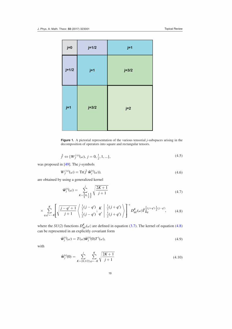
Figure 1 is a pictorial description of how various elements of these non-square tensors appear in the decomposition of f on j-sectors.

4.2. Generalized kernel

For the operators of equation (4.3), a convenient SU(2) covariant Wigner-like mapping to c-number functions, depending on three Euler angles , ,( )ω φ θ ψ=


Topical Review

19

ω⇔ =f W j, 0, , 1, ... ,fj s 1

2ˆ ( ) ( ) (4.5)

was proposed in [49]. The j-symbols

W fTr ,fj s

jsw( ) ( ˆ ˆ ( )) ( ) ( )ω ω= (4.6)

are obtained by using a generalized kernel

K

j

2 1

1js

K

j

0, 12

w

ˆ ( )( ) ∑ω =++

= (4.7)

j q

j

j q

j q

K

q

j q

j qD T

1

1; ,

q q K

Ks

qqK

Kq

j q j q

,

1

21

2

1

21

2

12

12

( )

( )

( )

( )( ) ˆ ( ) ( )

⎡

⎣⎢⎢

⎤

⎦⎥⎥∑ ω×

− ++

−

−

+

+

′ ′

′ ′

′

′=−

−+ −

′′

′ ′

(4.8)

where the SU(2) functions DqqK ( )ω′ are defined in equation (3.7). The kernel of equation (4.8)

can be represented in an explicitly covariant form

T T0 ,js

jsw wˆ ( ) ( ) ˆ ( ) ( )( ) ( ) †ω ω ω= (4.9)

with

K

j0

2 1

1js

K

j

q K

K

0,1 2

w ( )( )

/ ∑ ∑=

++= =−

(4.10)

Figure 1. A pictorial representation of the various tensorial j-subspaces arising in the decomposition of operators into square and rectangular tensors.


Topical Review

20

j q

j

j q

j q

K

q

j q

j qT

1

1; .

s

K q

j q j q1

21

2

1

21

2

12

12

( )

( )

( )

( )ˆ ( ) ( )

⎛

⎝⎜⎜

⎞

⎠⎟⎟×

− ++

−

−

+

+

−+ −

(4.11)

We point out that 0j1w ( )( )− is not a diagonal rank-one tensor as in the SU(2) case of equa-

tion (3.8); nevertheless we have the relation

w( ) ˆ ( )/

( )∑ + = Φ Φ=

−j 1 0 ,j

j0,1 2,1,..

1 (4.12)

S S S2 1 , .S 0,1 2,/∑Φ = +

= …

∞

(4.13)

The kernels of equation (4.8) are Hermitian and normalized

∫ ∫ ∫πφ θ θ ψ φ θ ψ

+ π π πj 1

16d d sin d , ,j

s2 0

2

0 0

4w ( )( ) (4.14)

j

j

, integer,

0, half-integer.j 11

⎧⎨⎩

= + (4.15)

In addition, they satisfy the following trace and orthogonality conditions:

ω =⎧⎨⎩

jj

Tr1, integer,0, half-integer,j

sw( )ˆ ( )

( ) (4.16)

Tr , ,js

js

j j j,w w( ˆ ( ) ˆ ( )) ( )( ) ( )ω ω δ δ ω ω=′ ′−′ ′ (4.17)

where j j,δ ′ is the usual Kronecker symbol while ,j( )δ ω ω′ is the reproductive kernel

W Wd , .fj

j j j fj

,( ) ( ) ( )∫ ω ω δ ω ω δ ω=′ ′′′

′ (4.18)

that functions as an analog of the δ-function on the group. Here, d d sin d dω φ θ θ ψ= is the SU(2) volume element.

It follows from equation (4.17) that the map (4.6) is explicitly invertible:

fj

W1

16d ,j f

j sj

s2

wˆ ( ) ˆ ( ) ( ) ( )∫π ω ω ω=+ − (4.19)

and thus establishes a one-to-one correspondence between the components f j appearing in equation (4.19) and the symbols W f

j s ( ) ( ) ω on the subspaces labeled by j.For every fixed value of the discrete parameter j, the map of equation (4.6) is a function of

three Euler angles and thus cannot be a representation of operators in a classical phase space, which by definition is even-dimensional. Nevertheless, in contrast with the standard SU(2) covariant Stratonovich–Weyl approach, the generalized map offers the possibility of recon-structing, through equations (4.4) and (4.19), the whole operator rather than only its projection on irreducible subspaces.

We note that, when f acts in a single SU(2) subspace, q 0=′ in equation (4.4), j is an inte-

ger and only square tensors T Kqj j2 2ˆ / /

enter in the map of equations (4.5) and (4.6). In this case

we recover the standard Stratonovich kernel of equation (3.8) with S = j/2, where w ,S js

2ˆ ( )/( ) θ φ= ,

is independent of the third angle ψ.


Topical Review

21

The kernel wSsˆ ( )( ) Ω of equation (3.8) is simply related to the generalized kernel j

sw ( )( ) ω of equation (4.8) by averaging over the angle ψ:

wd

4.S j

sjs

20

4wˆ ( ) ˆ ( )/

( ) ( )∫ψπ

ωΩ =π

= (4.20)

The physical significance of the phase ψ will be discussed in greater details later.The overlap relation can be seen to take the form

f gj

W WTr1

16d .

jfj s

gj s

0, 12

,12

( ˆ ˆ) ( ) ( ) ( ) ( )∫∑ πω ω ω=

+

= …

∞−

(4.21)

The symbol of the identity operator 1 on the entire space is obviously

1( ) Z∑ω δ= = ∈

= …

∞ ∗⎧⎨⎩W

j1 ,0 otherwise

j

njn

0,1,2 (4.22)

This implies the normalization condition

( ˆ ) ( )∫∑ πω=

+Θ

= …

∞

fj

WTr1

16d .

jfj

0,1,2,2 (4.23)

An explicit differential form for the star-product acting directly on j-symbols,

W W WL ,fgj s

j jf gj j j s

fj s

gj s

,,,

1 2

1 2 1 2( ) ( ( ) ( )) ( ) ( ) ( ) ( )∑ω ω ω= (4.24)

can be found in [73] and is reproduced in appendix C. It has a local form L f gj j j s

j j j j,,

, ,1 2

1 2

( ) δ δ∼ and reduces to the standard product of equation (B.1) when the operators f and g are elements of the enveloping algebra of su(2).

The structure of the correspondence rules (Bopp operators) for the generalized ker-nels is not unexpectedly more involved than for the simple SU(2) mappings of equations (3.40)–(3.41): derivatives with respect to the angle ψ appear even for the description of the action of the angular momentum operators [100]. The asymptotic form of correspondence rules are most useful in practice.

4.3. Some examples

Broadly speaking the generalized symbols W fj s ( ) ( ) ω have more complicated form than their

standard Stratonovich–Weyl expressions. In addition, not all of them have an intuitive inter-pretation, as can be seen from equation (4.29) below. Nevertheless, within the framework of this generalized formalism, one can find using equations (4.5)–(4.9) images of operator that do not belong to the su(2) enveloping algebra. This becomes especially attractive in the semi-classical limit, when these symbols ‘become functions defined’ in a symplectic phase space. We emphasize that the index j can only take integer values for symbols independent of ψ. When there is no ψ dependence, the operators act exclusively within an SU(2) irreducible subspace, and are functions of the angular momentum operators.

For instance, the image of the total angular momentum operator J2ˆ is

Wj j

2 21

Jj s

nj n,2 ( )( )

Z⎜ ⎟⎛⎝

⎞⎠ ∑ω δ= +∈ +

(4.25)

and independent of the parameter s.


Topical Review

22

On the other hand, non-diagonal tensors constructed as per equation (4.2) which mix SU(2) irreps always depend on the angle ψ, both for integer and half-integer values of of the index j.

For instance the operator n coszˆ θ= , corresponding to the z-component of the unit vector of equation (3.15), has an expansion in terms in the non-squared tensors of (4.2) as

nj

T T1

2,z

j

j j j j

1,3,5...10

12

12

10

12

12ˆ

⎛

⎝⎜⎜

⎞

⎠⎟⎟∑=

+−

=

+ − − +

(4.26)

and can also be expanded in a coordinate basis as

n d sin d cos , , ,zˆ ⟩⟨∫ ϕ ϑ ϑ ϑ ϕ ϑ ϕ ϑ= | | (4.27)

Y j m, , , ,j m j

j

jm0,1,

⟩ ( ) ⟩∑ ∑ϕ ϑ ϕ ϑ| = |= … =−

∗ (4.28)

where ϕ and ϑ are angles in the configuration space. The j-symbol for nzˆ is then obtained as

Wj

j 1sin cos .n

j ss

nj n

2

0,1,..,2 1z

( )( )/⎛

⎝⎜

⎞⎠⎟ ∑ω θ ψ δ=

+

−

=+ (4.29)

The counter-intuitive form of this symbol will be discussed later.Introducing the bi-polar spherical harmonics [93] Y Y, , Kq1 1 2 2 ( ) ( )ϕ ϑ ϕ ϑ⊗ ′ , one may

observe that for j Z∈ +, the kernel of (4.11) can be expressed for s = 0 using the , ⟩ϕ ϑ| basis as

0 d d , ,j0

1 2 2 2 1 1w ( )( ) ∫ ϕ ϑ ϕ ϑ= Ω Ω (4.30)

K

jY Y

2 1

11 , , .

K

j

q K

K j q

j q j q

Kq0

22

1 12

2 2( ) ( ) ( )⎧⎨⎩

⎫⎬⎭∑ ∑ ϕ ϑ ϕ ϑ×

++

− ⊗= =−

−+ − (4.31)

This representation clearly reveals its the angular momentum coupling nature of the mapping kernel.

As another example consider the realization of angular momentum states JM⟩| in terms of boson operators (the Schwinger representation):

⟩ ( ˆ ) ( ˆ )( ) ( )

⟩ ⟩† †

|+ −

| |+ −

J Ma b

J M J M,

! !0 0

J M J M

(4.32)

The boson annihilation operator a clearly connects JM⟩| and J M ⟩| ′ ′ , where J J 1

2= −′ and

M M 1 2/= −′ . Using equation (4.32) the Heisenberg–Weyl annihilation operator a can be expanded as

aj j

T1 2 3 2

2,

j

j j

12

, 32

,1 2 1 2

12

1 2 , 12

1 2ˆ ( / )( / ) ˆ

/ /( / ) ( / )

∑=+ +

= …−− +

(4.33)

and its symbol is given by

Wj j

j

1 2 3 2

1cos

1

2e ,a

j ss

sk

j k

1

1i 2

12

, 32

,

,( / ) ( / )

( ) ( ) ( )/ ∑θ δ=

+ ++

φ ψ−

−− +

= …

∞

(4.34)


Topical Review

23

showing that only half-integer values of j survive for this essentially ‘quantum’ operator. This should be contrasted with nzˆ , an operator that admits a classical interpretation.

An important application is to the product of two Heisenberg–Weyl coherent states

αβ α β=: ,a b (4.35)

/ ∑γγ

= γ−

=

∞

nne

!,

n

n2

0,1,..

2

(4.36)

This state is decomposable into a direct sum of the SU(2) coherent states S, ;0 0 ⟩θ φ| equa-tion (3.4) as

( )⟩/∑αβ θ φ= |ψ

= …

∞− r

SSe

2 !e , ; ,

S

rS

j

0, 12

,1,

22

i0 0

20

(4.37)

with the coherent state parameters α and β are given by

r rcos1

2e , sin

1

2e .0

i 20

i 20 0 0 0( )/ ( )/⎜ ⎟ ⎜ ⎟⎛⎝

⎞⎠

⎛⎝

⎞⎠α θ β θ= =φ ψ φ ψ− + − (4.38)

The sum over S clearly points to the existence of non-diagonal elements in the SU(2) decom-position of the density matrix ⟩⟨αβ αβ| |, so the standard map of equation (3.8) cannot be used. Within the generalized approach one calculates that the j-Wigner symbols of the sate equation (4.37) depend only on a single continuous parameter:

( )( ) ( )

( )( )

∑ω χ ν=

++

+ + −αβ

−

=

Wr

j

K

j K j K

e

1

2 1

1 ! !,j

j r

K

jK0

2

0, 12

2

(4.39)

where K( )χ ν is the SU(2) group character

Ksin 2 1

sin,K 2

2

( )[( ) ]

χ ν =+ ν

ν (4.40)

with the angle ν implicitly given by

ν θ θ φ φ ψ ψ

θ θ φ φ ψ ψ

= − − −

− + − −

cos cos cos cos

cos sin sin .

1

2

1

2 01

2 01

2 0

1

2 01

2 01

2 0

( ) ( ) ( )

( ) ( ) ( )

(4.41)

The corresponding Q-function also has a simple form:

( )( )( ) ( )

( ) ( )∑ω θ=+ −

′′ ′

αβφ ψ− −

=−

+

′

′ ′ ′W rj q j q

e cos1

! !e ,j r

j

q j

jq1 1

2

22i2

(4.42)

where the angles , ,(ω φ θ ψ=′ ′ ′ ′) are obtained as a composition 0ω ω of the Euler angles 0ω (4.38) and ω in the standard way [93].

4.4. Semiclassical limit

In the semi-classical limit, when typical values of the index j are sufficiently large, the exact expression of equation (4.24) for the star-product reduces to the elegant form


Topical Review

24

W

W W

e

d d

4e e ,

fgj s s s

j j

j j Jfj s j j J

gj s

12 2

0

4

2,

i i

0 0

1 2

20

1 10

2

( )

( )

( ( ))( ( ))

( ) ( ) ( ) ( )

( ) ( ) ( ) ( )

J J J J J J J J J J

∫ ∑

ω

ϕ ϕπ

ω ω

≈

×′

ε ε ε

πϕ ϕ

− ⊗ − ⊗ − ⊗ − ⊗ + ⊗

− + − −′

+ − − + + − − +

(4.43)

with

ie i cot1

sin, i .i 0J J

⎡⎣⎢

⎤⎦⎥θ

θψ θ φ ψ

=∂∂±

∂∂

∂∂

= −∂∂

ψ± ∓∓ (4.44)

More precisely, this semi-classical limit corresponds to situations where components with large values of j1 and j2 are the most important in the decomposition of the operators f and g given by equation (4.4). Since j J J1 1 1= + ′ and j J J2 2 2= + ′ , this occurs when J1′ and J1, and when J2′ and J2, are large in equation (4.3).

Operationally, the tensors appearing in the expansion of equation (4.4) should be predomi-nantly of low rank. When the density matrices satisfies this criteria, it describes so-called semi-classical states. The semi-classical parameter j 1 1( )ε = + − in this case is different in every sector labelled by the index j.

The approximate expression for the star-product given in equation (4.43) is considerably simplified in the limit where we consider j as a formal continuous parameter. Since symbols with integer and half-integer values of the index j behave in fundamentally different ways, the star-product takes a slightly different form in the continuous limit.

For integer j one can show that, to leading order in the semiclassical parameter, one obtains

ε

ε θ ε θ

ε

≈ ⊗ + ∂ ⊗∂ +

+ ∂ ⊗ ∂ +∂ − ∂ +∂ ⊗∂ +

+ + −∂ ⊗ + ⊗∂

ψ ψ

ψ θ θ ψ

+ +

+ +

+ + + +

W W W W W

W W W W

P W W W W W W

i cot cot

i2

,

fgj s

fj

gj

fj

gj

j j fj

gj

fj

gj

fj

gj

fj

gj j j

fj

gj

1 2 1 2

1 2 1 2

1 2 1 2 1 2 1 2

1 1

1 1

( )( )

( )

( )( )( ) ( )

ˆ

( ) / /

/ /

/ / / /

(4.45)

whereas, for the half-integer j case we have instead

ε

ε θ ε θ

ε

≈ ⊗ + ∂ ⊗∂ +

+ ∂ ⊗ ∂ +∂ − ∂ +∂ ⊗∂ +

+ + +⊗∂

+∂ ⊗

ψ ψ

ψ θ θ ψ

+ +

+ +

+ + + +

W W W W W

W W W W

P W W W W W W W W

i cot cot

i2 2

,

fgj s

fj

gj

fj

gj

j j fj

gj

fj

gj

fj

gj

fj

gj j

fj

gj j

fj

gj

1 2 1 2

1 2 1 2

1 2 1 2 1 2 1 2

1 1

1 1

( )( )

( )

( )( )( ) ( )

ˆ

( ) / /

/ /

/ / / /

(4.46)

where P is the Poisson bracket operator on 2S given in equation (3.32). Both of these expression contain derivative w/r to the parameter j, which is now understood in this limit to be continuous.

The form of the star-product given above can be used to obtain the semi-classical evo-lution equation for the j-symbols of the density matrix. Summing and extracting (4.45) and (4.46) one obtains the approximate Moyal equation (2.29) (to leading order in ε) for the linear combinations

W j W W, :s j s j s1 2( ) ( ) ( )( ) ( ) / ( )ω ω ω= ±ρ ρ ρ+

± (4.47)

in a form of [73] analogous to the standard TWA for the pure SU(2) case, given in equation (3.31)


Topical Review

25

( ) ( )( )

( )

( ) ( ) ( )

( )

( ) ( )

ωθ

θ

ω ω

∂ ≈ −+

∂ ⊗∂ −∂ ⊗∂ ++

∂ ⊗∂ −∂ ⊗∂

+ ∂ ⊗∂−∂ ⊗∂

ρ θ ψ ψ θ θ φ φ θ

ψ ψ ρ

±

± ±

⎡⎣⎢

⎤⎦⎥

W jj j

W j W j

,2 cot

1

2

1 sin

2 , , ,

ts

j j Hs s

(4.48)

which we can represent as a Poisson bracket on a 4-dimensional manifold:

ω ω ω∂ ≈ρ ρ± ± ±W j W j W j, 2 , , ,t

sHs s( ) ( ) ( )( ) ( ) ( )

(4.49)

W j W j, ,,

a b

ab Hs

a

s

b, 1

4 ( ) ( )( ) ( )

∑ ωω

ξ

ω

ξ=

∂

∂

∂

∂ρ

=

± ± (4.50)

W j W j W j, : , , ,Hs

Hj s

Hj s1 2( ) ( ) ( )( ) ( ) / ( )ω ω ω= ± +

± (4.51)

with j, , ,1 2 3 4ξ φ ξ θ ξ ψ ξ= = = = ; here, abω are the components of a non-degenerate closed 2-form ω:

j j1 d 1 cos d ,( ) ( )α ψ θ φ= + − + (4.52)

dω α= − (4.53)

d j d jd 1 cos d 1 .(( ) ) ( )φ θ ψ= ∧ + + ∧ + (4.54)

The (continuous) index j thus emerges as a new dynamical variable conjugate to the angle ψ.The canonical (Darboux) pairs j, 1 cos( ( ) )φ θ+ and j, 1( )ψ + can be conveniently inter-

preted in terms of a rigid rotor motion [99]: the projection j 1 cos( ) θ+ of the angular momen-tum j + 1 on the fixed axis z produces a phase shift φ, while the precession of the phase ψ is generated by total angular moment j + 1 in the body-fixed frame.

The 2-form ω of equation (4.54) defines a metric on the cotangent bundle T 2∗S corre-sponding to the co-adjoint orbit of the E(3) group fixed by the values of the Casimir opera-tors R 12 = and S R 0⋅ = , where the (commuting) generators of translations X Y ZR , ,( ˆ ˆ ˆ)= together with the components of the angular momentum operators S S SS , ,x y z( ˆ ˆ ˆ )= close on e(3), the Euclidean algebra in three dimensions:

S S S X X S X X, i , , 0, , i .i j ijk k i j i j ijk k[ ˆ ˆ ] ˆ [ ˆ ˆ ] [ ˆ ˆ ] ˆε ε= = = (4.55)

The translations operators X X Yiˆ ˆ ˆ= ±± and Z act on the angular momentum basis functions by multiplying the spherical harmonics Y ,jm( )ϕ ϑ by factors of sin e iϑ ϕ± and cosϑ, respectively.

We note that W 0j sS R( )( ) ω =⋅ while

( )( )Z

ω =∈

= …

+

⎪

⎪⎧⎨⎩

Wj

j

1 ,

0 , .j sR 1

2

3

2

2 (4.56)

As a result of the explicitly covariant form of the kernel given in equation (4.31), the semi-classical approach on T 2∗S is very convenient to study the dynamics of spin–spin interactions invariant under global rotations. For instance, given the Wigner j-symbol of L N Sz z zˆ ˆ ˆ= + and N Sˆ ˆ⋅ as

( )ω θ= +⎜ ⎟⎛⎝

⎞⎠W

j j1

2 2 21 cos ,L

jz (4.57)


Topical Review

26

Wj j

N N S S1

2 2 21 1 1 ,j

N S( ) ( ) ( )ˆ ˆ ⎜ ⎟

⎡⎣⎢

⎛⎝

⎞⎠

⎤⎦⎥ω = + − + − +

⋅ (4.58)

the dynamics resulting from the Hamiltonian

H N S N S,z zˆ ˆˆ ( ˆ ˆ )κ χ= + + ⋅ (4.59)

is described by the following simple evolution equation in the T 2∗S phase space:

W j W j j W j, , 2 1 , ,t ( ) ( ) ( ) ( )ω κ ω χ ω∂ = − ∂ − + ∂ρ φ ρ ψ ρ (4.60)

where no higher order derivatives appear. It follows from the solution of Equation (4.60)

ω φ κ θ ψ χ|− = − − + | =ρW j t W t j t j t, , , 2 1 , 0 ,( ) ( ( ) ) (4.61)

that the evolution of the angle ψ is different in each j-subspace and is an indicator of appear-ance of spin–spin correlations; this therefore represents an alternative to other correlation measures such as purity or negativity.

The correspondence rules (Bopp operators) are also nicely simplified in the semi-classical limit j 1 : to 1( )O one obtains [100]

W W1

2

1sin e ,S

j s j si( ) ¯ ( )( ) ( )J⎡⎣⎢

⎤⎦⎥ω

εθ ω≈ −ρφ

ρ++ (4.62)

W W1

2

1sin e ,S

j s j si( ) ¯ ( )( ) ( )J⎡⎣⎢

⎤⎦⎥ω

εθ ω≈ +ρ

φρ

−−− (4.63)

W W1

2

1cos i ,S

j s j sz

( ) ( )( ) ( )⎛⎝⎜

⎞⎠⎟ω

εθ

φω≈ −

∂∂ρ ρ (4.64)

where the operators J± are defined slightly differently from the J± equation (C.4): here we have

J θφ θ θ ψ

=∂∂+∂∂±

∂∂

φ±

± ∓⎡⎣⎢

⎤⎦⎥

ie cot i1

sin.i (4.65)

On the other hand, for HW creation-annihilation operators we obtain,

W W2

e cos 2 ,aj s j si

2

12( ) / ( )( ) ( )

ωε

θ ω≈ρ

φ ψρ

−+ +

(4.66)

W W2

e cos 2 ,aj s j si

2

12( ) / ( )( ) ( )

† ωε

θ ω≈ρ

φ ψρ

+ − (4.67)

indicating that, to leading order, the action of generators of the Heisenberg–Weyl algebra is reduced to a change the value of the index j by 1/2.

5. Applications to kinematical problems

5.1. Quantum tomography

One of the simplest applications of the theory of quasi-distributions for spin-like systems is an explicit reconstruction scheme of the density matrix from measured probabilities (see e.g. [15, 86] and references therein). For fixed spin systems one has


Topical Review

27

Sw Q

2 1

4d , , ,S

12

ˆ ˆ ( ) ( )( )∫ρπ

θ φ θ φ=+

Ω ρS

(5.1)

where

Q S S S S, , , , ,( ) ⟨ ˆ( ) ⟩θ φ ρ θ φ= | |ρ (5.2)

D D, , , .ˆ( ) ˆ ( ) ˆ ˆ( )†ρ θ φ θ φ ρ θ φ= (5.3)

The quantities Q ,( )θ φρ are frequently called tomograms.As mentioned in connection with equation (2.23), a direct tomographic reconstruction of

the SU(2) Wigner function

( ) ( ) ( )∫′π

Ω =+

Ω Ω Ω Ω′ρ ρS

WS

Q K4

2 1d , ,S

2

(5.4)

∑ ζΩ Ω′ ==

KS

S

L S

SP, ;

0cos ,S

L

S

L0

2

( ) ( ) (5.5)

with PL(z) the Legendre polynomial and ζ defined in equation (3.19), can be more appropri-ate especially for large values of the effective spin S (in which case the kernel ( )Ω Ω′K ,S is a smooth function) and/or when the precise value of S is unknown (due—say—to a weak depend ence of the kernel equation (5.5) on the spin size when S 1 ) [101].

Tomographic schemes like the ones mentioned above are highly redundant and in practice are discretized. For instance, the density matrix of spin S system can be recovered by measur-ing probabilities to obtain the maximum spin projection for (2S + 1)2 appropriately chosen direction [102]. On the other hand, the coefficients Kqρ of the multipole expansion (3.16), can

be found from the moments n S⟨( ) ⟩⋅

, K1 ⩽ ⩽ measured in suitable directions.The SU(2) maps are widely used for the tomography of two polarization modes (H and

V) within polarization sectors [76] constituted by states with fixed photon numbers and thus corresponding to SU(2) invariant subspaces. This kind of reconstruction of the polarization density matrix (in each subspace) can be efficiently performed in experiment [103] and the results can be conveniently represented as a distribution on the S2 sphere.

In the case of systems with variable spin or having a variable number of excitations, the reconstruction relation of equation (4.19) can be rewritten as [104]

jQ

1

16d ,

j

jj

0,1 2,12

1wˆ ( ) ˆ ( )/

( )∫∑ρπ

ω ω ω=+

ρ= …

∞

(5.6)

where ω ω ρ ω= =ρ=−

Q W QTr 0jjs j1( ) ˆ ( ) ( ˆ( ) ˆ ( )), where T Tˆ( ) ˆ ( ) ˆ ˆ ( )†ρ ω ω ρ ω= is the SU(2)-

transformed density matrix. In other words, the full density matrix can be reconstructed by measuring the expectation values of the operators (written in the angular momentum basis):

ˆ ( ) ( ) ( ) ( ) ( )∑= + + − −=−

Q j q j q j q j q0 , , .j

q j

j1

2

1

2

1

2

1

2 (5.7)

on ˆ( )ρ ω .One example of a variable spin system important in applications is the two polarization mode

states (H and V), considered in the whole space, and not only inside individual polarization sectors. In this case the operator Q 0

jˆ ( ) takes the specific form (in the photon polarization basis)


Topical Review

28

Q j q j q0 0 0 ,j

q j

j

HH VVˆ ( ) ∑= + − ⊗

=− (5.8)

with factorized states always containing the vacuum in one mode. Then, the data required for reconstruction of the complete state of an arbitrary two-mode polarized light field can be obtained from a conditional balanced homodyne tomographic setup [104].

5.2. Phase distribution problem

5.2.1. SU(2) relative phase POVM. The map (3.8) can be used to introduce a distribution function for the phase φ associated with the projection of the angular momentum on the z axis. In quantum optics, the phase φ is frequently related to the relative phase between polarization modes [105] defined in each polarization sector. Such an operator valued measure (POVM) can be defined [105, 106] by integrating over θ the kernel of the equation (3.8) for s = −1, corresponding to the Q-function

Ω = |Ω Ω |=−w S S; ; ,Ss 1ˆ ( ) ⟩⟨( ) (5.9)

where S; ⟩|Ω is the SU(2) coherent state (3.4). The phase POVM

Sw

2 1

4d sin ,S S

0

1ˆ ( ) ˆ ( )( )∫φπ

θ θ∆ =+

Ωπ

− (5.10)

is positively defined, Hermitian, normalized

, d ,S S S

0

2

1ˆ ( ) ˆ ( ) ˆ ( )†

∫φ φ φ φ∆ = ∆ ∆ =π

(5.11)

and satisfies the covariance condition,

e e .SS

SS

i i0

z z0 0ˆ ( ) ˆ ( )ˆ ˆφ φ φ∆ = ∆ +φ φ− (5.12)

The resulting probability distribution

P Tr S( ) [ ˆ ( ) ˆ]φ φ ρ= ∆ (5.13)

can be used to evaluate averages of phase observables according to

f P fd .0

2( ˆ) ( ) ( )∫φ φ φ φ=

π (5.14)

Although in many situations the explicit form of (5.13) is quite complicated, the asymp-totic for S 1 frequently is notoriously simplified. For instance, for a coherent state (3.4)

S;0 ⟩|Ω one has

PL

Sexp

2 1, 0 ,

2

0 0( )ˆ

( )⎛

⎝⎜⎜

⎞

⎠⎟⎟φ δ φ φ θ π≈ −

+− < < (5.15)

where L2ˆ is the differential realization of the Casimir operator on 2S . For 00θ ≠ or π the opera-

tor L2ˆ , when acting on 0( )δ φ φ− , is reduced to

L1

sin,

2

20

20

ˆθ

= − ∂φ (5.16)

while at 00θ = or π (i.e. for highest and lowest states ⟩| ±S S, of the representation), it leads to a flat distribution: P 1 2( ) /φ π= . Then, for instance, for typical angle observables we obtain


Topical Review

29

L

Scos exp

2 1cos .k k

2

0

ˆ⎛

⎝⎜⎜

⎞

⎠⎟⎟φ φ= −

+ (5.17)

In the contraction limit described in equations (3.46)–(3.50), the POVM equation (5.10) is reduced to the phase distribution operator for the Heisenberg–Weyl group, which also allows to consistently define the phase operator itself [107].

5.2.2. Joint ψ φ− POVM. The map of equations (4.6)–(4.8) allows a generalization of the concept of phase distribution to systems with variable spin. The phase ψ in this case is formally one of the angle variables defining a point in j, , ,( )φ θ ψ space. As discussed in section 4.4 this phase also appears in the semi-classical limit as a variable conjugate to j, and thus can be inter-preted as a phase shift generated by the total angular momentum rather than to its projection on a given fixed axis. Algebraically, the phase ψ carries information about coherences between sectors (labelled by j) of a density matrix. Thus, in the framework of the generalized SU(2) approach one can introduce a joint φ-ψ POVM in a way that generalizes equation (5.10):

j,

1

16sin d ,

jj

0, 12

,1,..2 0

1wˆ ( ) ˆ ( )( )∫∑φ ψπ

θ θ ω∆ =+ π

=

− (5.18)

where j1w ( )( ) ω− is defined in equation (4.8), and the positivity of (5.18) follows from (4.13).

The operator ,ˆ ( )φ ψ∆ is normalized

d d , ,0

4

0

21ˆ ( )∫ ∫ψ φ φ ψ∆ =

π π (5.19)

and covariant under Sz rotations,

e , e , ,S Si iz zˆ ( ) ˆ ( )ˆ ˆφ ψ φ φ ψ∆ = ∆ + ′φ φ− ′ ′ (5.20)

and S0ˆ -displacements,

e , e , ,S Si i0 0ˆ ( ) ˆ ( )ˆ ˆφ ψ φ ψ ψ∆ = ∆ + ′ψ ψ− ′ ′ (5.21)

where the operator

S N N k N k1

22, 2, ,

N k N

N

00,1,... 2

2ˆ / /

/

/

∑ ∑==

∞

=− (5.22)

plays the role of the total photon number in the case of two-polarized field modes; S0ˆ also

commutes with the angular momentum operators. Integration of ,ˆ ( )φ ψ∆ over ψ gives a direct sum of SU(2) phase POVM given in equation (5.10):

d , .j

j0

4

0,1,2

ˆ ( ) ˆ ( )/∫ ∑ψ φ ψ φ∆ = ∆π

= …

∞

(5.23)

The average values are computed by using the joint probability distribution function P , Tr ,( ) [ ˆ ( ) ˆ]φ ψ φ ψ ρ= ∆ in the standard manner:

f g P f gd d , ,0

2

0

4( ˆ) ( ˆ) ( ) ( ) ( )∫ ∫φ ψ φ ψ φ ψ φ ψ=

π π (5.24)

and in general f g f g .( ˆ) ( ˆ) ( ˆ) ( ˆ)φ ψ φ ψ≠


Topical Review

30

For the two-mode coherent state of equation (4.35), where in the parametrization of equa-tion (4.38) the angle 0ψ plays the role of ‘phase’ between SU(2) irreducible subspaces (4.37), the joint distribution function in the limit of large average photon number, α β| | + | | = n 1,2 2 ¯ has the asymptotic form,

P , e ,nJ 20 0

2( ) ( ) ( )/φ ψ δ φ φ δ ψ ψ≈ − −− (5.25)

where

J1

sin2 cos ,2

20

20

20 0 0 0

( )θ

θ= − ∂ − ∂ ∂ +∂φ φ ψ ψ (5.26)

so that in particular,

cos e cos , cos e cos ,k n k k n kJ J20

20

2 2ˆ ˆ/ /φ φ ψ ψ≈ ≈− − (5.27)

have sharp maxima at 0ψ and 0φ , while the correlation disappears for high intensity fields

O ncos cos e cos cos cos cos 1 .nJ 20 0

2ˆ ˆ ( ) ˆ ˆ ( / )/φ ψ φ ψ φ ψ≈ = +− (5.28)

Observables depending only on the phase ψ can be computed using a POVM obtained by integrating equation (5.18) over the phase φ,

d , ,0

2ˆ ( ) ˆ ( )∫ψ φ φ ψ∆ = ∆π

(5.29)

which satisfies the covariance condition (5.21), but it is not invariant under the action of Sz. In the particular case of the state equation (4.37) one has

P Je ,1

sin.nJ 2

02

20

22

0( ) ( )/ψ δ ψ ψ

θ≈ − = − ∂ψ− (5.30)

6. Applications to semi-classical dynamics

In this section we present some examples of semi-classical dynamics using the Truncated Wigner Approximation for spin-like systems with fixed and variable values of spin. In general, the TWA is appropriate for description of dynamics of semi-classical states represented in phase space as smooth localized functions, the typical size of which is much less than char-acteristic dimensions of the classical potential, and located in stable regions of the symbol of Hamiltonian. In addition, the TWA can also describe evolution of states located in unstable classical regions, although the time scale for the validity of this description is necessarily shorter than for the stable motion. This more limited validity is related to a comparatively larger sensitivity to small fluctuations leading to a faster deviation from classical trajectories.

The main effect captured by TWA is a deformation of the initial distribution, since different points in the distribution move with different velocities (with the exception of evolutions gen-erated by Hamiltonians linear in the generators, for which the evolution of the state amounts to a rigid translation in phase space of the original function). Physical effects such as e.g. spin squeezing [108] which arise from this type of Hamiltonian are well described in the TWA and thus are purely classical in nature in the sense that all ‘quantumness’ of this effect is in the initial distribution rather than in the evolution.

The situation becomes more interesting for multipartite systems. Here, the semi-classical evolution occurs in a phase space which is a direct product of phase spaces of individual sub-systems. The semi-classical evolution may then ‘entangle’ the interacting subsystems in the


Topical Review

31

sense that the initially independent distributions associated with different physical subsystems become strongly interrelated without affecting the purity of the initial state. In this case there may exists more than one semi-classical parameter.

The semi-classical time semτ for which the TWA describes relatively well the quantum evolution of higher order correlation functions of spin observables, strongly depends both on the Hamiltonian and the initial state. In many physical applications the (dimensionless) semi-classical time is semτ ε∼ λ− , 0 1⩽λ< , where ε is a semi-classical parameter. Interestingly, for some selected observables the time validity of the TWA can be significantly longer than the semi-classical time semτ . In the case of spin-variable systems the semi-classical parameter is usually taken as averaged over the sectors that have the largest contribution in the decomposi-tion of the initial state.

The possibility of simulating the full quantum dynamics by semi-classical dynamics can be fruitfully applied for optimization purposes; for instance, to the determination of optimum values of the interaction constants needed to achieve the best squeezing or entanglement in spin-like systems.

Finally, we note that one important ingredient of the semiclassical approach is that the Wigner function of the physically relevant initial states (such as coherent states, squeezed states, etc) can be nicely approximated in the limit S 1 using the asymptotic form of the mapping kernel given in equation (3.23). The asymptotic form of the kernel eliminates numer-ical errors appearing in the computation of Clebsch–Gordan coefficients for representations of large dimensions.

6.1. Fixed S dynamics

Suppose the density matrix decomposes into SU(2)-invariant subspaces as in equation (2.20). Then, in each invariant subspace the semi-classical dynamics is governed by classical trajec-tories on 2S :

( ) ( ( ) ( ) )θ φ θ φ| = − − | =ρ ρW t W t t t, , 0 , (6.1)

where t t,( ) ( )θ φ are solutions of the classical Hamiltonian equations and W W, : ,0( ) ( )( )θ φ θ φ=ρ ρ .The time scale semτ for which TWA remains valid is heavily dependent on the highest

degree of the polynomial in the su(2) generators entering in the Hamiltonian. For typical phys-ical applications where interaction Hamiltonians are no more than quadratic in the generators and assuming the interaction constant χ of the highest degree operator is independent of the SU(2) irrep label S , the TWA usually fails before τ ∼ −Ssem

1 2/ and τ ∼ −Ssem1 for stable and

unstable regimes, respectively. Nevertheless, typical observables such as some average values and fluctuations of the spin operators, may evolve according to the semi-classical picture even up to times τ∼ 1 , where the quantum interference effects become predominant and in general cannot be neglected.

6.1.1. The finite Kerr-like interaction. The simplest non-trivial example is the Kerr-like Hamiltonian

H S .z2ˆ ˆχ= (6.2)

The symbol of the Hamiltonian is given in table 1 as

( )θ φ θ∝W , cosH2 (6.3)


Topical Review

32

and leads to the following evolution of the Wigner function [57, 109, 110]:

θ φχε

θΩ| = − | =ρ ρ⎜ ⎟⎛⎝

⎞⎠W t W

tt, cos 0 ,( )

(6.4)

i.e. parts of the initial distribution located at different values of θ precess with different angular velocities about the z axis.

If the initial state is the equatorial coherent state of (3.27), with 2, 00 0/θ π φ= = , so the phase space distribution is localized at the stable fixed point of W cosH

2( ) θΩ ∼ , the solution to equation (6.4) leads to a very good description of squeezing effect: the first and the second moments of the spin operators are described up to times t 1χ ∼ . By contrast, the evolution of arbitrary observables is usually well described by TWA, in this particular case, only up to times Ssem

1 2/χτ − . For longer times, telltale signs of self-interference leading to Schrödinger cats on the sphere start to appear, as can be noticed for instance by analyzing the behaviour of the fourth moment m4(t) of the Wigner function using Equation (2.39).

6.1.2. The Meshkov–Lipkin interaction. The TWA is also applicable to the less trivial case of the Meshkov–Lipkin interaction [111]:

H S gS .z x2ˆ ˆ ˆχ= + (6.5)

The semi-classical (i.e. large angular momentum) trajectories of this Hamiltonian have been by investigated by Bohr and Mottelson in the context of the nuclear cranking model [113].

The resulting symbol for the Hamiltonian is given by

W gsin cos

2

cos

4.H

2

2( ) θ φ

εχ θε

Ω = + (6.6)

This Hamiltonian can be seen to exhibit a second order phase transition for gε χ= .When the initial state is a spin coherent state 2, 00 0/ ⟩θ π φ| = = located at the minimum

of WH( )Ω given in equation (6.6), the corresponding truncated evolution equation leads to the standard equations for ( ,θ φ)

g sin ,tθ φ∂ = − (6.7)

g cot cos cos ,tφ θ φχε

θ∂ = − + (6.8)

providing a good description of the time-dependence of the two first moments of the angu-lar momentum operators below the phase-transition point g ⩽ε χ up to times t Sχ λ− ,

1 2/λ< . Above the phase-transition point, gε χ> , the same state 2, 0/ ⟩π| is on the classical separatrix but the evolution of the first two moments is still sufficiently well approximated for

t S , 1 2/χ λ∼λ− even in this unstable regime [112].The deviation of the semi-classical evolution from the exact evolution of the fourth order

moment m4 of equation (2.39) is quite different above and below the phase transition: below the transition, when g ⩽ε χ, the semi-classical approximation hold to Ssem

1 2/χτ − whereas above, when gε χ> it holds to Ssem

1χτ − .

6.1.3. Bi-partite systems. For bi-partite systems, when the Wigner distribution is defined on 2 2×S S , the evolution along classical trajectories leads to inter-dependence of phase variables

in the individual sub-manifolds, which results in a strong correlation between interacting sub-systems. This effect can be observed even on the simplest example of bi-linear interaction


Topical Review

33

H S S ,z z1 2ˆ ˆ ˆ( ) ( )

χ= ⊗ (6.9)

which leads to the following evolution of the bi-partite Wigner function in the TWA [57]:

W t Wt t

t, ,2

cos ; ,2

cos 0 ,1 2 1 12

2 2 21

1( ) ( )θ φχε

θ θ φχε

θΩ Ω | = − − | =ρ ρ (6.10)

( )ε = + −S2 11,2 1,21 (6.11)

Equation (6.10) provides an excellent description of the purity dynamics P(t) of one of inter-acting spins

( ) ( ) ( ) ( )∫ρ= ∼ Ω Ω Ω′ Ω Ω | Ω Ω′ |ρ ρP t W t W tTr d d d , , ,12

1 2 2 1 2 1 2 (6.12)

frequently used for the characterization of the spin–spin entanglement for pure states.Since purity is not a physical observable, the limitations for its applicability are not the

same as for moments of the angular momentum operators. In particular, the results of TWA basically coincide with exact quantum computations for large spins [57] for arbitrary times.

In situations where the spin–spin interaction is modified by the presence of a magnetic field, the interaction Hamiltonian has more complicated structure:

H S S g S S ,z z y y1 2 1 2 1 2

1 1ˆ ˆ ˆ ( ˆ ˆ )( ) ( ) ( ) ( ) ( ) ( )

χ= ⊗ + ⊗ + ⊗ (6.13)

and in particular reveals a phase transition at g2 ε χ= . The TWA describes well a short time evolution of bi-partite correlations even in the unstable regime and can be used for optim-ization of spin–spin entanglement as a function of the parameter g/χ in the limit of large spins.

Finally, we add the TWA also describes the long-time dynamics of some other properties of multi-partite systems, such as the negativity [71], which characterizes spin–spin correla-tions [112].

6.2. Variable spin dynamics

Following equations (4.50)–(4.54), the semi-classical dynamics of a quantum system with variable spin—or alternatively systems for which the initial state contains non-neg-ligible contributions from several large SU(2) subspaces—is defined by trajectories in the four-dimensional symplectic manifold T 2∗S . These trajectories can be different for

W j W W,s j s j s1 2( ) ( ) ( )( ) ( ) / ( )ω ω ω= ±ρ ρ ρ+

±. The computation of average values of operators

containing only T KQˆ ′

tensors for + =′ even in its decomposition (and in particular the

square tensors describing operators from the su(2) enveloping algebra) is completed using

W Wj j1

2( ( ) ( ))ω ω+ρ ρ+ −

:

T jj

d1

16KQ0 2

ˆ ∫ π=

+∞′ (6.14)

W jW t j t W t j t

d ,, ,

2,

T KQ ( )

( ( ) ( )) ( ( ) ( ))∫ ω ω

ω ω×

− − + − −ρ ρ+ −′ (6.15)

where t( )ω and j(t) are classical trajectories on T 2∗S .For the expectation values of non-squared tensors, for which + =′ odd, we need to use

W W Wj j j1 2 1

2( ) ( ( ) ( ))/ ω ω ω= −ρ ρ ρ

++ − :


Topical Review

34

T jj

d1

16KQ0 2

ˆ ∫ π=

+∞′ (6.16)

W jW t j t W t j t

d ,, ,

2,

T KQ ( )

( ( ) ( )) ( ( ) ( ))∫ ω ω

ω ω×

− − − − −ρ ρ+ −′ (6.17)

where n n1 2,/ Z− = + ∈′ .There are two basic physical situations for which the semi-classical picture on T 2∗S is

appropriate, depending if the expansion of the Hamiltonian contains only square tensors, or rectangular and square tensors.

6.2.1. Hamiltonian with square tensors only. If the decomposition of the Hamiltonian con-tains only square tensors so H is block-diagonal, and if an exact or perturbative solution in each SU(2)-subspace is available, the whole evolution operator is recovered by summing over irreducible subspaces with coefficients from the initial state expansion.

On the other hand, the density matrix will typically contain contributions from multiple subspaces, its phase space image, in general, will contain non-square tensors coupled by the Hamiltonian: the evolution of the density matrix is not a simple sum of maps in each SU(2)-irreducible subspace.

This is where decomposing in terms of j-sectors becomes particularly convenient: whereas various SU(2)-subspaces of Wρ may be mixed, different j-sector are NOT mixed under evo-lution: when the Hamiltonian is block-diagonal and preserves irreducible SU(2)-subspaces the Wigner function evolves in each j-sector as

W t W t t t j, , , , ,j( ) ( ( ) ( ) ( ) )ω φ θ ψ θ φ| = − − + Ψ |ρ ρ (6.18)

where t t,( ) ( )θ φ are classical trajectories on 2S and the form of j t, ,( )θ φΨ | depends on the Hamiltonian function.

For instance, it follows readily from equation (4.25) that the total angular momentum, H J

2ˆ ˆω= , generates only rotations of the ψ-angle in the (integer) j-symbols,

( ) ( ( ) )ω φ θ ψ ω| = − + | =ρ ρW t W j t j t, , 1 , 0 .j (6.19)

As another example, consider the non-linear two-mode Hamiltonian

H a a b bg

a b ab2 2

,2 2ˆ (( ˆ ˆ) ( ˆ ˆ) ) ( ˆ ˆ ˆ ˆ )† † † †χ= + + + (6.20)

that preserves the integral of motion N a a b bˆ ˆ ˆ ˆ ˆ† †= + and can be recast, up to the constant

operator N N J11

2

1

2

2ˆ ( ˆ ) ˆ+ ≡ representing the total angular momentum, in terms of the su(2)

algebra generators in form of the Lipkin-Meshkov model given in equation (6.5), with

S a b ab S a a b b1

2,

1

2.x z

ˆ ( ˆ ˆ ˆ ˆ ) ˆ ( ˆ ˆ ˆ ˆ)† † † †= + = − (6.21)

If the initial state belongs to a single SU(2) irrep, the approximation given in equation (6.1) can be applied in the limit of large average excitation numbers N⟨ ˆ ⟩.

For an arbitrary initial state, for instance the product of coherent states given in equa-tion (4.35) which does not belong to a single SU(2) subspace, where at least one of the fields is in a strong coherent state, the evolution equation on T 2∗S should be used. The angle ψ in the general solution (6.18) then evolves according to


Topical Review

35

t j t g2

31

cos

sind .

t

0( ) ( ) ( )

( )∫ψ ψ χφ τθ τ

τ= + + + (6.22)

We should point out that it is not always convenient to use a map from a two-mode Hamiltonian into an su(2) form because of the complexity of computing the symbol of the Hamiltonian. For instance, a direct application of the generalized map of equations (4.6) and (4.8) and in particular of equation (4.34) is more appropriate in the case of the down-conver-sion Hamiltonian,

H g a b b a .2 2ˆ ( ˆ ˆ ˆ ˆ )† †= + (6.23)

The j symbol of this Hamiltonian contains only half-integer j and for j 1 simplifies to

( ) ( ) ( )/ω θ θ φ ψ≈ + +W j2 1 cos sin cos 3 ,Hj 3 2 2 1

2

1

2

1

2 (6.24)

while the representation of (6.23) in terms of su(2) generators contains square roots and their Wigner symbols do not have simple expressions.

Solutions in the form equation (6.18) should be used for computation of averages of non-squared operators, as for instance, a a,ˆ ˆ† in case of equation (6.5) or (6.23).

6.2.2. Hamiltonians containing non-square tensors. Suppose the expansion of the Hamil-

tonian of the system contains non-square operators T KQˆ ′

, ≠ ′ . A simple physical situation

where this would occur consists e.g. in adding to an SU(2) invariant two-mode Hamiltonian a (non-invariant) pumping term ∼ a a( ˆ ˆ)†+ .

For this type of Hamiltonian the two-mode Heisenberg–Weyl TWA does not always lead to satisfactory results, especially when one of the non-linearly coupled field is initially in a vac-uum state. This kind of system cannot be treated in terms of the standard Stratonovich–Weyl approach either, but is tractable in the formalism of generalized j-mappings [100].

As an example of this situation, we consider the Lipkin–Meshkov Hamiltonian of equa-tion (6.20) in the presence of external pumping a a( ˆ ˆ)†µ + .

In this case, the evolution of both W j,( )ωρ+ and W j,( )ωρ− are required. The evolution of W j,( )ωρ+ yields Hamilton equations defining classical trajectories on T 2∗S :

tg

d

dsin ,

θφ= − (6.25)

tg j

d

dcot cos 1 cos ,( )φθ φ χ θ= − + + (6.26)

tg j

d

d

cos

sin

2

31 ,( )ψ φ

θχ= + + (6.27)

j

tj

d

d2 1 cos

1

2sin

1

2.( ) ( ( ))µ θ φ ψ= − + + (6.28)


Topical Review

36

The first two equations are similar to (6.7) with j 11 →ε +− but now contain an evolution of the index j.

The evolution of W j,( )ωρ− is obtained with minimal effort by changing →µ µ− in equa-tion (6.28), with the other Hamilton equations remaining the same.

As in the single-S SU(2) case, the initial Wigner function can be well approximated in the limit j 1 . For instance, the Wigner function corresponding to the state r0⟩ ⟩α β| = | = in the limit of a highly excited b-mode, r 12 has the form

ω

ω ν

=

=

∈ρ

ν

ρν

− − −

+ − − −

+

⎫

⎬⎪⎪

⎭⎪⎪

Wj

r

W

j2 e e ,

2e e cos ,

,

j j r r j

j j r r j

22 2 sin 1

2

1 2 2 2 sin 12

1

2

2 2 2 2

2 2 2 2

( )

( )

( ) / ( )

/ ( ) / ( )Z (6.29)

where

ν θ φ ψ= −cos sin cos .1

2

1

2

1

2( )( ) (6.30)

6.3. The linear rigid rotor

The linear rigid rotor is an example of a system for which typical Hamiltonians contain non-square tensors. This example deserves a separate treatment due to its importance in many applications, such as linear molecules in external fields.

To connect with Classical Mechanics, we need a change of coordinate so that the symmetry axis of the rotor (rather than the total angular momentum axis) is now the quantization axis. This is achieved by first applying a 2/π -rotation about the y-axis. Applying this rotation to the kernel of equation (4.11) yields

0 e 0 e .jy S Si 2 i 2y yw wˆ ( ) ˆ ( )/ ˆ / ˆ= π π− (6.31)

The full kernel

T T0jy

jyw wˆ ( ) ( ) ˆ ( ) ( )†ω ω ω= (6.32)

leads to the standard classical picture [114]. This can be verified by noting for instance that, with this change of axis, the symbol of nzˆ operator (4.27) has now an intuitive form

W jcos .nj

nj n

0,1,..,

1z( ) ( )∑ω θ δ≈ +

=

−O (6.33)

This should be compared with the ‘unrotated’ expression of equation (4.29).The Darboux coordinates become p ,( )θθ and p ,( )φφ , where the conjugate momenta to

coordinates θ and φ are

p j 1 sin ,( ) ψ= +θ (6.34)

p j 1 sin cos ,( ) θ ψ= +φ (6.35)

and p 0=ψ always.Using this scheme a simple semi-classical approach to linear rigid rotor evolution can be

developed, as for instance, the alignment dynamics in an external field described by

H J n .z2 2ˆ ˆ ˆκ= − (6.36)


Topical Review

37

To leading order in 1/j, the j-symbol is just a classical Hamiltonian

W jj j

,2 2

1 cos ,Hj 2( ) ⎜ ⎟

⎛⎝

⎞⎠ω κ θ= + − (6.37)

where j takes only integer values. The truncated Wigner evolution for W j,( )ωρ leads to the fol-lowing evolution:

j 1 sin ,t ( )θ ψ∂ = − + (6.38)

j 1cos

sin,t ( )φψθ

∂ = − + (6.39)

jj

1 cot cos4 cos sin cos

1t ( )ψ θ ψ

κ θ θ ψ∂ = − + +

+ (6.40)

j 4 cos sin sin ,t κ θ θ ψ∂ = (6.41)

which are equivalent to the standard Hamilton equations for the canonical variables p ,( )θθ and p ,( )φφ and describe well the alignment dynamics for times t 1κ ∼ . Alternative phase space-

like approaches were developed in [115].

6.4. Dissipation

As a final application we consider the semi-classical dynamics of dissipative systems, gov-erned by the Lindblad equation:

H Li , ,tj

j jˆ [ ˆ ˆ] ˆ ( ˆ)∑ρ ρ γ ρ∂ = − + (6.42)

where Ljˆ is a Lindblad superoperator.Phase space methods allow the rewriting (sometimes exactly as for HW symmetry, or to

some approximation in the SU(2) case) of the Lindblad equation in the form of a diffusion equation, thus helping the analysis of physical effects using the intuitive language of classical mechanics [116, 117].

In the semi-classical limit of the TWA, the Schrödinger equation is mapped to the classi-cal Hamiltonian equation (in the sense that the image of the commutator is the appropriate Poisson brackets), so that zeroth order terms in a semi-classical parameter appearing in the expansion of the star-product of equations (3.28), (4.45) and (4.46) (or of the correspondence rules of equations (3.40), (3.41), (4.62)–(4.64)) cancel out.

As a result of this cancellation, the star-product is not formally required in order to obtain the evolution equation in the semi-classical limit within the framework of the standard clas-sical phase space approach. To represent the action of the superoperators Ljˆ in phase space, both zeroth and first order terms in the semi-classical expansions (3.40), (3.41), (4.62)–(4.64) are needed.

The dissipative phase-space dynamics of spins were studied quite intensively using mainly the P- and Q-symbols. The Wigner map is sometimes more convenient for physi-cal analysis [118]; the evolution equation takes a slightly different form than for the P- and Q-representations. Here, we provide a few equations appearing in typical spin relaxation problems.


Topical Review

38

6.4.1. Single spin systems. When the system is in equilibrium with a thermal bath at temper-ature T and limited to a single value of S, the dissipative terms are given by

L S S S S S Sg

2 ,1

2,1 1 1

ˆ ( ˆ) ( ˆ ˆ ˆ ˆ ˆ ˆ ˆ ˆ ˆ ) ( )ρ γ ρ ρ ρ γ

ν= − − =

+− + + − + − (6.43)

where kTexp 101ħ[ ( / ) ]ν ω= − − and

L S S S S S Sg

2 ,2

,2 2 2ˆ ( ˆ) ( ˆ ˆ ˆ ˆ ˆ ˆ ˆ ˆ )ρ γ ρ ρ ρ γ

ν= − − =+ − − + − + (6.44)

with g a system-bath effective coupling. The Lindblad equation (6.42) was discussed in the framework of the SU(2) phase-space approach in numerous papers (see for instance [41] [117] [118] and references therein). The evolution equation for the Wigner function is obtained by using the semi-classical expansion of the correspondence rules for the su(2) generators:

L 2 cos sin1,22

2

21ˆ ( ˆ) → ( )

⎡⎣⎢

ρφ

ε θ θ− −∂∂

+ ∂θ−∓L (6.45)

W2

2 1 cos3

2

2 1

4sin .2

2

( ) ( )⎛

⎝⎜

⎛⎝⎜

⎞⎠⎟

⎞

⎠⎟⎤

⎦⎥⎥

εθ θ± + + +

+∂ Ωθ ρL

L (6.46)

with L is given in equation (3.34).A contribution from a dispersion-like decoherence

L S S S S2

2dd

z z z z2 2ˆ ( ˆ) ( ˆ ˆ ˆ ˆ ˆ ˆ ˆ )ρ

γρ ρ ρ= − − (6.47)

takes the form of a phase-diffusion differential operator:

LW

.d

2

2ˆ ( ˆ) →

( )ρ

φ∂ Ω

∂ρ

(6.48)

In the high temperature limit where 1ν , we find the simplified expression for the super-operator image in the phase space:

ρν

ρν

φ+ − +

∂∂

Ωρ⎛⎝⎜

⎞⎠⎟L L L W

2 2.1 2

22

2ˆ( ˆ) ( ˆ ˆ )( ˆ) → ( )L (6.49)

6.4.2. Multiple S values. In this case a contribution from the S0ˆ operator, defined in equa-

tion (5.22) and such that S S 120 0

ˆ ( ˆ )= +L may arise in order to describe a decoherence between different invariant subspaces. This effect appears in the description of depolarizing channel in two-mode system:

L S S S S2

2 .s 0 0 02

02ˆ ( ˆ) ( ˆ ˆ ˆ ˆ ˆ ˆ ˆ )ρ ρ ρ ρ=

Γ− − (6.50)

In this case the phase space dynamics is described by

LW j,

.s

2

2ˆ ( ˆ) →

( )ρ

ωψ

∂

∂ρ

(6.51)


Topical Review

39

7. Generalizations: SU(n) mappings

7.1. The general case

The formalism of Stratonovich–Weyl maps can be fairly easily generalized to some systems with SU(n) dynamical symmetry. A straightforward construction of an s-parametrized w sˆ ( )( ) Ω mapping kernel for systems with SU(n) symmetry group was proposed in [32] and contains certain ambiguities. An accurate deduction of such kernel for symmetric representations of SU(n) has been done in [23] (see also [81, 122]).

Denote by H the Hilbert space of a quantum system. Suppose a compact Lie group G, which we take to be SU(n) acts irreducibly on H so that H carries the irrep λ of G. Elements ω∈G act linearly in H via the matrix representation T ( )ω .

Let H be the largest subgroup of SU(n) that leaves ; h.w.⟩λ| invariant (to within a phase), and the phase space for the corresponding classical system is isomorphic to the coset

SU n( )/M H= [83], so that SU(n) acts on M by canonical transformations.Operators acting in H will transform according to the irrep λ λ⊗ ∗, where λ∗ the irrep con-

jugate to λ.The product λ λ⊗ ∗ is reducible so, in addition to the labeling of states in irrep λ, we must

consider the labeling of tensors from a general irrep , , ..., n1 2 1( )σ σ σ σ= − . In general, a weight α in irrep σ may occur multiple times; the label Iα distinguishes between multiple occurrences of this weight.

Ambiguities occur when the irrep σ occurs more than once in the decomposition λ λ⊗ ∗, and how to proceed in such cases remains an open question [23].

Assuming σ is not repeated in the decomposition λ λ⊗ ∗, a tensor T I;ˆγσλ

γ is given

explicitly by

T I I C; ; ,II I

I II

; ;ˆ ⟩⟨ ˜∑ α βλ λ= | |γ α β

γσλ

α βα β λ λ

σγ

α β

α β

γ∗∗ (7.1)

where λ∗ the irrep conjugate to λ, β∗ the weight conjugate to β, and σ an irrep in the decom-position of λ λ⊗ ∗.

The coefficients C I II

;˜α βγλ λσ

α β

γ∗ ∗ satisfy the orthogonality relation

C CI I

I II

I II

I I; ;( ˜ ) ˜∑ δ δ δ=α βν

α βν

ννα β

λ λσ

λ λσ

σσ∗

′′

′ ′′ ′

α β

α βν

α β

νν ν

∗ ∗ ∗ ∗ (7.2)

and are elements of a unitary matrix. The irreducible tensors of equation (7.1) satisfy

h T T, .i I i I; ;[ ˆ ˆ ] ˆα=α ασλ

σλ

α α (7.3)

which implies the tensors are trace orthogonal over ,ασ and Iα:

T TTr .I I I I; ;[( ˆ ) ˆ ] δ δ δ=α ασλ

σλ

σσ αα∗

′ ′′ ′ ′ ′ ′ ′α αα α

(7.4)

For SU n( ) irreps of the type , 0, , 0( )λ … , basis states will be written ; ⟩νλ| , where the ith component of the weight , , n1 1[ ]ν ν ν= … − is the eigenvalue of the ith Cartan element on the state:

h ; ; .i iˆ ⟩ ⟩ν νλ ν λ| = | (7.5)


Topical Review

40

For these irreps there is no weight multiplicity and the additional label I is not necessary. Moreover, an irrep σ occurs at most once in λ λ⊗ ∗, where 0, ,( )λ λ= …∗ . Thus, for instance:

⊕λ λ σ σ⊗ = σλ= SU, 0 0, , for 3 ,0( ) ( ) ( ) ( ) (7.6)

SU, 0, 0 0, 0, , 0, for 4 , etc.0( ) ( ) ( ) ( )⊕λ λ σ σ⊗ = σλ= (7.7)

The highest weight vector of , 0, , 0( )λ … is U n 1( )− invariant; this subgroup acts only on the last n − 2 components of a weight. The kernel is then of the form

w F D T ,s s

II I0; 0 ;ˆ ( ) ( ) ˆ( ) ( )∑ ∑Ω = Ω

ββ βλ

σσ

σσλ

β

β β (7.8)

with

D I T 0; ; 0 , ,I 0; 0( ) ⟨ ( ) ⟩ Mβσ σΩ ≡ | Ω | Ω∈βσ

ββ (7.9)

an SU n( ) group function for the irrep , 0, , 0,( )σ σ σ≡ … [119], and

F Cdim

dim.s

ss0

1 2

h.w.; h.w.0( )

( )( ˜ )( )

( )/⎡⎣⎢

⎤⎦⎥

σλ

=σ λ λσ

+−

∗ ∗ (7.10)

Here, the notation 00 is meant to imply that the state 0; 0⟩σ| has zero-weight and is a scalar (invariant) under U(n − 1) transformations.

7.2. The case of SU 3( ) irreps of the type λ, 0( )

For the simplest non-trivial example of the SU(3) group, the general equations (7.8)–(7.10) can be further developed. We follow [119] for the labeling and construction of basis states for an irrep ,( )λ µ . Defining

C a a a a ,ij i j i j1 1 2 2ˆ † † † †= + (7.11)

the Lie algebra su(3) is spanned by the six ladder operators C i j, 1, 2, 3ij ˆ ≠ = together with the two diagonal Cartan elements

h C C C h C C2 , .1 11 22 33 2 22 33ˆ ˆ ˆ ˆ ˆ ˆ ˆ= − − = − (7.12)

The root diagram is given in figure 2. Basis states are then given by

∑

λ µ ν ν ν

ν ν ν λ

λν ν ν

|

= | | |

I

m m

I

N

I

N mm m m

,

; ; ,m m m N

1 2 3

1

2 3

3

1

2 2

2

1

2 1

1

1

21

2

1

2 1 11

2 2 21

2 3 3

1 2 3

( )( ) ⟩

⟩ ⟩ ⟩( )

(7.13)

⟩( ˆ ) ( ˆ )( ) ( )

⟩† †

| =+ −

|+ −

s ma a

s m s m! !0 .i i

is m

is m

i i i i

1 2i i i i

(7.14)

with ;j

m

j

m

J

M1

1

2

2 an SU(2) Clebsch–Gordan coefficient.

The weight ,1 2 2 3[ ]ν ν ν ν ν≡ − − of the state is extracted from a triple 1 2 3( )ν ν ν of non-nega-tive integers constrained by 21 2 3ν ν ν λ µ+ + = + . The label kν is seen, from equations (7.13) and (7.14), to be the total number of quanta in mode k of a 3-dimensional oscillator with two


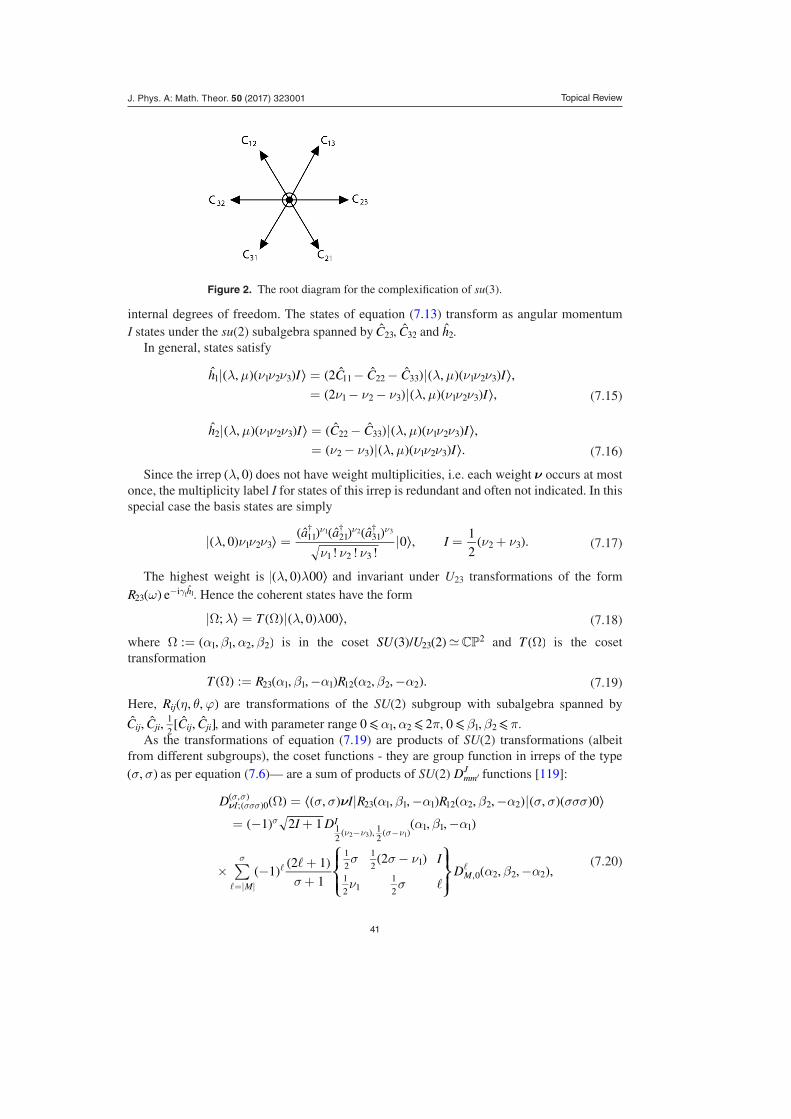
Topical Review

41

internal degrees of freedom. The states of equation (7.13) transform as angular momentum I states under the su(2) subalgebra spanned by C23

ˆ , C32ˆ and h2

ˆ .In general, states satisfy

ˆ ( )( ) ⟩ ( ˆ ˆ ˆ ) ( )( ) ⟩( ) ( )( ) ⟩

λ µ ν ν ν λ µ ν ν νν ν ν λ µ ν ν ν

| = − − |= − − |

h I C C C I

I

, 2 , ,

2 , ,1 1 2 3 11 22 33 1 2 3

1 2 3 1 2 3 (7.15)

λ µ ν ν ν λ µ ν ν νν ν λ µ ν ν ν

| = − |= − |

h I C C I

I

, , ,

, .2 1 2 3 22 33 1 2 3

2 3 1 2 3

ˆ ( )( ) ⟩ ( ˆ ˆ ) ( )( ) ⟩( ) ( )( ) ⟩ (7.16)

Since the irrep , 0( )λ does not have weight multiplicities, i.e. each weight ν occurs at most once, the multiplicity label I for states of this irrep is redundant and often not indicated. In this special case the basis states are simply

a a aI, 0

! ! !0 ,

1

2.1 2 3

11 21 31

1 2 32 3

1 2 3

( ) ⟩( ˆ ) ( ˆ ) ( ˆ )

⟩ ( )† † †

λ ν ν νν ν ν

ν ν| = | = +ν ν ν

(7.17)

The highest weight is , 0 00( ) ⟩λ λ| and invariant under U23 transformations of the form R e h

23i 1 1( ) ˆω γ− . Hence the coherent states have the form

T; , 0 00 ,⟩ ( ) ( ) ⟩λ λ λ|Ω = Ω | (7.18)

where : , , ,1 1 2 2( )α β α βΩ = is in the coset SU U3 2232( )/ ( ) CP and T ( )Ω is the coset

transformation

T R R: , , , , .23 1 1 1 12 2 2 2( ) ( ) ( )α β α α β αΩ = − − (7.19)

Here, R , ,ij( )η θ ϕ are transformations of the SU(2) subgroup with subalgebra spanned by

C C C C, , ,ij ji ij ji1

2ˆ ˆ [ ˆ ˆ ], and with parameter range 0 , 21 2⩽ ⩽α α π, 0 ,1 2⩽ ⩽β β π.

As the transformations of equation (7.19) are products of SU(2) transformations (albeit from different subgroups), the coset functions - they are group function in irreps of the type

,( )σ σ as per equation (7.6)— are a sum of products of SU(2) DmmJ′ functions [119]:

( ) ⟨( ) ( ) ( ) ( )( ) ⟩

( ) ( )

( ) ( ) ( )( )

( )( )

( ) ( )

∑

νσ σ α β α α β α σ σ σσσ

α β α

σ

σ σ ν

ν σα β α

Ω = | − − |

= − + −

× −++

−−

ν σσσσ σ

σν ν σ ν

σ

− −

=| |

⎧⎨⎪

⎩⎪

⎫⎬⎪

⎭⎪

D I R R

I D

ID

, , , , , , 0

1 2 1 , ,

12 1

1

2, , ,

I

I

MM

; 0,

23 1 1 1 12 2 2 2

12

, 12

1 1 1

1

2

1

2 1

1

2 11

2

,0 2 2 2

2 3 1

(7.20)

Figure 2. The root diagram for the complexification of su(3).


Topical Review

42

with M 1ν σ= − and a b cd e f

⎧⎨⎩

⎫⎬⎭ an su(2) 6j-symbol [119]. The measure dΩ on the coset and

the range of integration of the parameters are given by

∫ ∫ ∫ ∫ ∫α α β ββ β

βΩ =−π π π π

d d d sin dd 1 cos

4sin .

0

2

20

2

10

1 10

2 22 (7.21)

The SU(3) tensor operators are constructed using SU(3) Clebsch–Gordan coefficients for the coupling , 0 0, ,( ) ( ) → ( )λ λ σ σ⊗ . Indeed we find

∑ λ α α α λ β β β

λα α α

λλ β λ β λ β

σ σν ν ν

= | |

×− − −

−

αβν ν νσ σ

λ β−

T

J

, 0 , 0

, 0;

0,

, ,

,

;1

J;,

1 2 3 1 2 3

1 2 3 1 2 3 1 2 3

1 2 3

2

ˆ ( ) ⟩⟨( )

( ) ( ) ( ) ( )

( )

(7.22)

where the SU(3) Clebsch–Gordan coefficient can be factored in the usual way as

J

, 0;

0,

, ,

,

;1 2 3 1 2 3 1 2 3

( ) ( ) ( )λα α α

λλ β λ β λ β

σ σν ν ν− − −

(7.23)

( ) ( ) ( ) ( )

( ) ( ) ( )λα

λλ β

σ σν

α α

α α

β

β β ν ν=

−

+

− − −J

J, 0;

0, ,

;; .

1 1 1

1

2 2 3

1

2 2 3

1

2 1

1

2 3 21

2 2 3

(7.24)

The coefficient λα

λλ β

σ σν−

;J

, 0 0, ,

;1 1 1

( ) ( ) ( ) is the reduced SU(3) CG, an expression for which is given

in equation (D.1) of the appendix.

Since dim , 0 1 21

2( ) ( )( )λ λ λ= + + and dim , 1 3( ) ( )σ σ σ= + the factor F s( )

σ of equa-

tion (7.10) specializes to:

F 1, 0

00;

0,

0

,

; 0

2 1

1 2,s

s s3 1 2

( ) ( ) ( ) ( ) ( )( )( )

( )( )/⎛

⎝⎜

⎞⎠⎟

⎛⎝⎜

⎞⎠⎟λ

λλλλ

σ σσσσ

σλ λ

= −+

+ +σλ

− +

(7.25)

λσ

λ σ λ σσ

λ λ= −

++ + −

++ +

λ

− +⎛

⎝⎜⎜

⎞

⎠⎟⎟

⎛⎝⎜

⎞⎠⎟1 !

2 1

2 ! !

2 1

1 2,

s s3 3 1 2

( ) ( )( ) ( )

( )( )( )

( )/

(7.26)

where we have used the expression for ( ) ( ) ( )λλ

λ σ σσ

;, 0 0,

0

,

; 0 given in equation (D.9) of the

appendix.These expressions allow a complete construction of the kernel w sˆ ( )( ) Ωλ of equation (7.8).

The Wigner-type symbols, s = 0, of some of the su(3) generators are provided in table 2.Average values are computed in the usual manner

A W W1 2

8d .A2

⟨ ˆ⟩ ( )( ) ( ) ( )∫λ λ

π=

+ +Ω Ω Ωρ (7.27)

Combining the expressions of equations (7.26) and (7.22) for F 0( )σ and T 0; 0

ˆσλ

, the Wigner kernel at 0Ω = takes the form


Topical Review

43

w F T0 ,00

0

0; 0ˆ ( ) ˆ( ) ( )∑=λ

σ

λ

σ σλ

= (7.28)

n n n n n n, 0 , 0 1 ,n n n

n n nn

1 2 3 1 2 3

1 2 3

1 2 31( ) ⟩⟨( ) ( )∑ λ λ= | | −

λ

λ

+ + =

C (7.29)

where n n n1 2 3 λ+ + = . On the other hand, for s = −1, the kernel at the origin simplifies to the expected form

ˆ ( ) ˆ ( ) ⟩⟨( )( ) ( )∑ λ λ λ λ= = | |λσ

σ σλ− −w F T0 , 0 00 , 0 00 .0

1 10 (7.30)

In the limit 1λ , the coefficient n n n1 2 3

λC can be approximated [23] as:

n

n n

0 if 3,

26

if 3,n n n

1

1 11 2 3

/

/

⎧⎨⎪

⎩⎪

λ

λλ

<

− + >λ C (7.31)

in a manner reminiscent of the asymptotic form of the SU(2) kernel at the origin given in equation (3.23).

Again in the 1λ regime, the Wigner symbol for the highest weight state , 0 00( ) ⟩λ λ| is well approximated by

W Ae ,cos 12( ) ( )Ω ≈ρλ β − (7.32)

where A is a normalization constant chosen so that

W1 2

8d 1

2

( )( ) ( )∫λ λ

π+ +

Ω Ω =ρ (7.33)

7.3. Some applications

An interesting application the general formalism presented in equations (7.8)–(7.10) is to the quantum tomography of systems with SU(n) symmetry. This can be done by a formal applica-tion of the reconstruction formula of equation (2.21). Several proposal for the implementa-tion of such protocols were discussed in [123–125], where additional delicate situations were analyzed. The reduction to the form equation (2.23) is also possible, although the general expression becomes quite cumbersome.

Another direct application is the problem of SU(3) relative phase POVM, similar to the corresponding SU(2) case considered in section 5.2.1. The POVM for two relative phases 1α and 2α can be obtained by integrating the kernel w 1ˆ ( )( ) Ωλ

− over ,1 2β β :

ˆ ( ) (( )) ˆ ( )( )∫ ∫α αλπ

β ββ β

β∆ =−

Ωπ π

λ−w,

dim , 0

4sin d

d 1 cos

4sin ,1 2 2 0

1 10

2 22

1 (7.34)

where the normalization factor is chosen so that

d d , .0

2

10

2

2 1 2 1ˆ ( )∫ ∫α α α α∆ =π π

(7.35)

Under shifts generated by the action of the Cartan operators the POVM equation (7.34) is transformed to


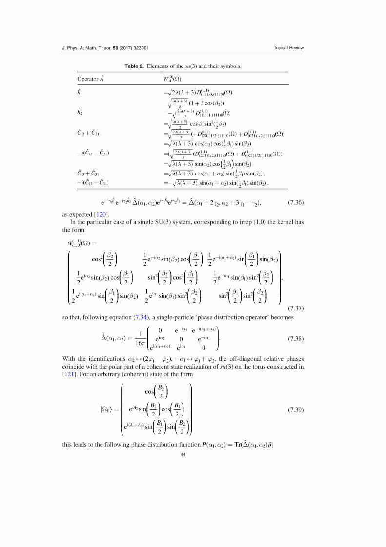
Topical Review

44

e e , e e 2 , 3 ,h h h hi i1 2

i i1 2 2 1 2

1 1 2 2 1 1 2 2ˆ ( ) ˆ ( )ˆ ˆ ˆ ˆα α α γ α γ γ∆ = ∆ + + −γ γ γ γ− − (7.36)

as expected [120].In the particular case of a single SU(3) system, corresponding to irrep (1,0) the kernel has

the form

ββ

β ββ

ββ β β

ββ

ββ β

β β β

Ω =

α α α

α α

α α α

−

− − +

−

+

⎜ ⎟ ⎜ ⎟ ⎜ ⎟

⎜ ⎟ ⎜ ⎟ ⎜ ⎟ ⎜ ⎟

⎜ ⎟ ⎜ ⎟ ⎜ ⎟ ⎜ ⎟

⎛

⎝

⎜⎜⎜⎜⎜⎜⎜

⎛⎝

⎞⎠

⎛⎝

⎞⎠

⎛⎝

⎞⎠

⎛⎝

⎞⎠

⎛⎝

⎞⎠

⎛⎝

⎞⎠

⎛⎝

⎞⎠

⎛⎝

⎞⎠

⎛⎝

⎞⎠

⎛⎝

⎞⎠

⎛⎝

⎞⎠

⎞

⎠

⎟⎟⎟⎟⎟⎟⎟

w

cos2

1

2e sin cos

2

1

2e sin

2sin

1

2e sin cos

2sin

2cos

2

1

2e sin sin

2

1

2e sin

2sin

1

2e sin sin

2sin

2sin

2

,

1,01

2 2 i2

1 i 12

i2

1 2 2 2 1 i1

2 2

i 12

i1

2 2 2 1 2 2

2 1 2

2 1

1 2 1

ˆ ( )

( ) ( )

( ) ( )

( ) ( )

( )( )

( )

( )

(7.37)so that, following equation (7.34), a single-particle ‘phase distribution operator’ becomes

,1

16

0 e ee 0 e

e e 0

.1 2

i i

i i

i i

2 1 2

2 1

1 2 1

ˆ ( )( )

( )

⎛

⎝

⎜⎜

⎞

⎠

⎟⎟α α

π∆ =

α α α

α α

α α α

− − +

−

+ (7.38)

With the identifications 22 1 2↔ ( )α ϕ ϕ− , 1 1 2↔α ϕ ϕ− + , the off-diagonal relative phases coincide with the polar part of a coherent state realization of su(3) on the torus constructed in [121]. For an arbitrary (coherent) state of the form

B

B B

B B

cos2

e sin2

cos2

e sin2

sin2

A

A A

0

2

i 2 1

i 1 2

2

1 2

⟩

( )

⎜ ⎟

⎜ ⎟ ⎜ ⎟

⎜ ⎟ ⎜ ⎟

⎛

⎝

⎜⎜⎜⎜⎜⎜⎜

⎛⎝

⎞⎠

⎛⎝

⎞⎠

⎛⎝

⎞⎠

⎛⎝

⎞⎠

⎛⎝

⎞⎠

⎞

⎠

⎟⎟⎟⎟⎟⎟⎟

|Ω =

+

(7.39)

this leads to the following phase distribution function P , Tr ,1 2 1 2( ) ( ˆ ( ) ˆ)α α α α ρ= ∆

Table 2. Elements of the su(3) and their symbols.

Operator A W A0 ( )( ) Ω

h1 = D2 3 111 0; 111 01,1( ) ( )( ) ( )

( )λ λ+ Ω

= 1 3 cos3

82( ( ))( ) β+λ λ+

h2ˆ = D2 3

3 111 1; 111 01,1 ( )( )

( ) ( )( )− Ωλ λ+

= cos sin3

21

2 1

2 2( )( ) β βλ λ+

C C12 21ˆ ˆ+ = D D2 3

3 201 1 2; 111 01,1

021 1 2; 111 01,1( ( ) ( ))( )

( ) / ( )( )

( ) / ( )( )− Ω + Ωλ λ+

= 3 cos cos sin21

2 1 2( ) ( ) ( ) ( )λ λ α β β+

C Ci 12 21( ˆ ˆ )− − = D Di 2 3

3 201 1 2; 111 01,1

021 1 2; 111 01,1( ( ) ( ))( )

( ) / ( )( )

( ) / ( )( )Ω + Ωλ λ+

= 3 sin cos sin21

2 1 2( )( ) ( ) ( )λ λ α β β+

C C13 31ˆ ˆ+ = 3 cos sin sin1 2

1

2 1 2( ) ( ) ( ) ( )λ λ α α β β+ + ,

C Ci 13 31( ˆ ˆ )− − = 3 sin sin sin1 21

2 1 2( ) ( ) ( ) ( )λ λ α α β β− + + ,


Topical Review

45

α α π α π α

π α α

= − + −

+ − − + + +

+ +

⎜ ⎟ ⎜ ⎟

⎜ ⎟ ⎜ ⎟ ⎜ ⎟

⎜ ⎟ ⎜ ⎟ ⎜ ⎟

⎛⎝⎜ ⎛

⎝⎞⎠

⎛⎝

⎞⎠

⎛⎝

⎞⎠

⎛⎝

⎞⎠

⎛⎝

⎞⎠

⎛⎝

⎞⎠

⎛⎝

⎞⎠

⎛⎝

⎞⎠⎞⎠⎟

P BB

A BB

A

BB A A

B B

B B B

,1

12sin sin

2cos sin cos

2cos

sin2

sin cos 4 sin2

sin2

4 cos2

4 sin2

cos2

.

1 2 12 2

1 1 21

2 2

12 1 2 1 2

2 1 2 2

2 2 2 2 2 1

( ) ( ) ( ) ( ) ( )

( ) ( )

(7.40)

7.4. SU(3) dynamics

7.4.1. Poisson bracket on SU U3 2 2( )/ ( ) CP . Following the general scheme presented in equations (2.28)–(2.32) the semi-classical dynamics of quantum systems with SU(3) sym-metry group is developed on SU U3 2 2( )/ ( ) CP , where the local coordinates are determined by the coset parametrization of equation (7.19) as , , ,1 1 2 2( )α β α βΩ = , and the semi-classical param eter is

1

2 3.

( )ε

λ λ=

+ (7.41)

One then obtains the Poisson bracket in the form [82]

,4

sin sin12 1

2 21 1 1 1 ( )

β β⋅ ⋅ = ∂ ⊗ ∂ −∂ ⊗∂α β β α (7.42)

2 tan

sin

1

2 1

2 1

2 22 1 1 2( )

β

β− ∂ ⊗∂ −∂ ⊗∂α β β α (7.43)

4

sin.

22 2 2 2( )

β+ ∂ ⊗∂ −∂ ⊗∂α β β α (7.44)

Although the SU(3) Wigner functions are not so conveniently illustrated on 2CP , the most important features of the evolution can be captured by analysis of physically meaningful lim-its in which some semiclassical trajectories can be obtained either analytically or numerically in the TWA scheme. In addition, additional insights can be gained by plotting projections of the Wigner function on some selected submanifolds [80, 82].

7.4.2. Application: two types of SU(3) squeezing. The simplest dynamical application of the SU(n) phase space approach is the analysis of squeezing, i.e. the possibility of reduc-ing quant um fluctuations of given observables in multi-level systems below some commonly accepted threshold. It can be shown [82] that an hierarchy of different types of squeezings can be established, caused by dynamically induced correlations between substructures in the spec-trum of the system. Analysis of these effects can be performed completely in the framework of the SU(n) TWA.

The simplest SU(3) Hamiltonians that lead to a deformation of an initial distribution result-

ing in squeezing are of the form H h1 12ˆ ˆ∼ + linear terms and H h2 2

2ˆ ˆ∼ + linear terms, where h1


Topical Review

46

and h2ˆ are given in equations (7.15) and (7.16). The the linear terms are added for conveni-

ence, to remove rigid rotations of the distribution in the phase space.The effect produced by these Hamiltonians is substantially different:

a) The Hamiltonian

H h h2 3

60,2

21ˆ ˆ ˆ⎜ ⎟

⎛⎝

⎞⎠

λ= +

+ (7.45)

with symbol

W1 3 4

480sin

1

23 4 cos 5 cos 2 20 1 3 cos 2 ,

H4

2

2 2 1

2

( ) ( )( )

[ ( ) ( ( ))]

⎜ ⎟⎛⎝

⎞⎠

λ λ λ λβ

β β β

=− + +

× + + + + (7.46)

generates evolution of the angles 1α and 2α

t t0 1 4 cos sin1

2,1 1 1

22( ) ( ) ( )( ) ⎜ ⎟

⎡⎣⎢

⎛⎝

⎞⎠⎤⎦⎥α α λ λ β β= − − + (7.47)

t t01

101 4 1 cos sin

1

2,2 2 1

22( ) ( ) ( )( ) ⎜ ⎟

⎡⎣⎢

⎛⎝

⎞⎠⎤⎦⎥α α λ λ β β= − − + − (7.48)

in a very similar way as the Hamiltonian H Sz2ˆ ˆ∼ leads to the phase φ dynamics in case of

SU(2) symmetry, as shown in equation (6.4). This is especially noticeable from how the sym-

bol W cos sinh 12 1

2 22 ( )β β∼ appears in equations (7.47)–(7.48). Since h2ˆ is the Cartan element

proportional to the operator Sz of the su23(2) subalgebra equation (7.17), h22ˆ produces SU(2)-

like correlations in each SU23(2) subrepresentation contained in the original , 0( )λ irrep. As a result, the optimal squeezing time and the maximum achievable squeezing scale with λ practically in the same way as they scale with S in spin systems [82].b) The Hamiltonian

H h h h C C C2 3

5, 2 .1

21 1 11 22 33ˆ ˆ ˆ ˆ ˆ ˆ ˆ⎜ ⎟

⎛⎝

⎞⎠

λ= −

+= − − (7.49)

with symbol

W9

401 3 4 3 4 cos 5 cos 2 ,H 2 2( ) ( )( ) ( ( ))λ λ λ λ β β= − + + + + (7.50)

produces, in contradistinction to equation (7.45), correlations between SU(2) subspaces but no correlations inside the subspaces, as h1 acts diagonally on SU(2) states. As a result, the type of

squeezing generated by H h12ˆ ˆ∝ is qualitatively different from SU(2)-type squeezing. This dif-

ference is reflected in the scaling behaviours with λ of optimal squeezing times and maximum squeezing. This type of squeezing can be considered as a pure SU(3) squeezing [82].

From the phase space perspective it is clear that since WH depends on 2β alone, the only coordinate to evolve in time, according to equation (7.44), will be 2α . For an initial state of the form

R B0, , 0 , 0 0012 2⟩ ( ) ( ) ⟩ζ λ λ| = | (7.51)

with B arccos 1 52 ( / )= − (which defines the location of the minimum of the potential function (7.50)), the trajectory can be obtained analytically as


Topical Review

47

t t09

51 4 1 5 cos ,2 2 2( ) ( ) ( )( ) ( )α α λ λ β= − − + + (7.52)

resulting in a squeezing of the initial distribution.

8. Conclusion

This review is a survey of the axiomatic formulation of phase space quantum mechanics, con-centrating on spin-like systems and following Stratonovich. Our aim was to highlight some of the uses of phase space methods in a variety of kinematical and dynamical settings, including situations where the states of the system contain more than one value of spin angular momen-tum and provide some explicit expressions ready for their immediate applications in particular physical situations.

The formalism for higher symmetry group can be generalized without too much difficulty but technology required for practical calculations—various Clebsch–Gordan and recoupling coefficients, the properties of coset functions etc—are still not well developed.

Because of the inherent breadth of applications, we have by design included many tech-nical results, but only references to source papers where fuller derivations and discussions can be found. We hope that in this way the review can serve a springboard for further invest-igations in a research area where new results are constantly published.

Acknowledgments

The work of ABK is supported by CoNaCyT grant 254127. The work of HdG is supported by NSERC of Canada. HdG would like to dedicate this review to the memory of Prof V V Paranjape.

Appendix A. An integral form of w 0Ssˆ ( )( )

One can show that

w 0 d e ,Ss S s

0

2i zˆ ( ) ( )( ) ˆ ( )∫ ω κ ω=

πω (A.1)

iL

S

S

S

L S

S

1

2

2 1

2 1;

0s

L

SL

LS

s

0

2

( ) ( ) ( )( ) ∑κ ωπ

χ ω= −++=

−

(A.2)

where LS( )χ ω are the generalized characters of the group [93]

iS

M

L S

Me ;

0.L

S L

M

Mi( ) ∑χ ω = ω− (A.3)

One can also show that the function 0 ( )( )κ ω in the limit case of large representation dimensions, S 1 takes the following asymptotic form [94] (see also [95]),

SS1

i, ,S0 ( ) → ( ) ( ) ( ) →( ) ⎡

⎣⎢⎤⎦⎥κ ω δ ω π

ωδ ω π− − −

∂∂

− ∞ (A.4)

where the limit is understood in a weak sense.


Topical Review

48

Appendix B. Exact expression for the SU(2) star-product

The SU(2) star-product operation can be expressed as

N a F F FL ,f g Sn

n Ss n

Ss

fn

Ss

g,1 2 1 2 1 2( ) ( ) [( ( )) ( ( )) ]( ) ( )S S∑Ω = ⊗− + − − −L L L (B.1)

where we have used the notation A B W W AW BW:f g f g f gˆ ˆ ( ) ( ˆ )( ˆ )⊗ = , and

[( ) ( ) ] /= + +N S S S2 1 2 1 ! 2 ! ,Ss 2 (B.2)

=−+ +

an S n

1

! 2 1 !.n

n( )( ) (B.3)

Here 2L is Casimir operator on the sphere given in equation (3.34) such that

F Y F L Y, , ,S L M S L M2

, ,( ) ( ) ( ) ( )θ φ θ φ=L (B.4)

with FS(L) succinctly given by

= + + −F L S L S L2 1 ! 2 ! ,S( ) ( ) ( ) (B.5)

but expressible as a function of L(L + 1). In other words

F F L L M L M, , .SL M

S2

,

( ) ( ) ⟩⟨∑= | |L (B.6)

The symbolic powers n( )S± have been introduced in (B.1) according to

( ) θθ

= Π − ∂ ∂θ φ±

=− ⎜ ⎟

⎛⎝

⎞⎠∓S k cot

i

sin.n

kn

01 (B.7)

The number of terms in the sum (B.1) is finite because the Wigner function ΩW fs ( )( ) of an

operator f is the polynomial of finite degree in the SU(2) generators: specifically

W n f0, deg ,nfs ( ) ˆ( ) ( )S Ω = >± (B.8)

where the degree of non-linearity, fdeg ˆ, (in the generators of the su(2) algebra) of an operator f , is defined by the maximum value of , such that f 0k ≠ , with f k given in equation (3.16).

As an example, the star-product for S = 1/2 is given by

Ω

= ⊗

− ⊗

+ − − −

− + − − −

⎜⎛⎝ F F F

F F F

L

21

2

,

f g

sSs

Ss

f Ss

g

Ss

Ss

f Ss

g

,

1 2 1 2 1 2 1 2

1

3 !1 2 1 1 2 1 1 2 )

( )

( ) [( ( )) ( ( )) ]

( ) [( ( )) ( ( )) ]

( )/

( ) ( )S S

L L L

L L L (B.9)

where F W 0fs1 2˜ ( ) ( ) =− L if fdeg 2ˆ ⩾ .

The s,0

( )Λ± operators for =±s 1 are given in equation (3.44). For the Wigner function (s = 0) they are quite involved,

θ θ θΛ = Φ − + ∂ Φε

εθ−cos cos 2 sin ,0

0 1

42

41 2( ) ( ) ( )( ) L L (B.10)


Topical Review

49

( ) [ ( )] ( )( ) L Lθε

θ θΛ = Φ ± − ± Φφ ε φ±

±±

± −l lesin

42 cos e sin 2 1 ,z

0 i 24

i 1 2 (B.11)

where the function ( )Φ L2 is given in equation (3.37) and 2L is the differential realization of the SU(2) Casimir operator (3.34).

Appendix C. Generalized star-product operation

The generalization of the star-product operation for an arbitrary value of of the ordering parameter s can be found following [49], leading to the following explicit expression:

1 1( )( )( )

( ˆ )( ( ˆ ) ( ˆ ))

[((ˆ ) ( ˆ ) ( ( ˆ ) ( ˆ )) )

((ˆ ) ( ˆ ) ( ( ˆ ) ( ˆ )) )]

( )ˆ ˆ

/

( ˆ ) /

( ˆ ) /

J J

J J J

J J J

J J

J

J

∫

⊗

∑ϕ ϕπ

=+ ++

× Γ − + Γ + +

× Γ − + Γ + +

Γ − + Γ + +

′π

ϕ

ϕ

=

∞

− ⊗ + ⊗

−

− −

+ − − +

− − − −

′

⎡⎣⎢

⎤⎦⎥

aj j

j

F J j j

F J j j

F J j j

Ld d

4

1 1

1

2 2

e 2 2

e 2 2 ,

f gj j j s

njn

s

js s

nj

s j j s

nj

s j j s

,,

0

4

20 2

1 2

12

1 2 0 0 2

1 2 i1

01

0 2

1 2 i2

02

0 2

1 20 0

12

0

21

0

(C.1)

where

=−

Γ + +a

n K n

1

! 2 2,K

nn( )

( ) (C.2)

( ˆ ) ( ) ( ) ( ) ( )Θ = + + − ΘF J D j k j k D1 ! ! ,j nmk

nmk2 (C.3)

x( )Γ is the standard Gamma-function, x x x1( ) ( )Γ + = Γ ,

ie i cot1

sin, i ,i 0ˆ ˆJ J

⎡⎣⎢

⎤⎦⎥θ

θψ θ φ ψ

=∂∂±

∂∂

∂∂

= −∂∂

ψ±∓∓ (C.4)

are the contravariant components of the su(2) algebra generators, and

J cot1

sin2 cos ,

22

2 2

2

2

2 2

2ˆ

⎡

⎣⎢

⎛⎝⎜

⎞⎠⎟⎤

⎦⎥

θθθ θ φ

θφ ψ ψ

= −∂∂+

∂∂+

∂∂−

∂∂ ∂

+∂∂

(C.5)

is the Casimir operator.

Appendix D. Reduced SU(3) CG coefficients λλ

λσ

σ σσ− − + −q p q p J

, 0;

0, ,2 ;

( ) ( ) ∥ ( )

We have found that the reduced SU(3) CG needed to construct the tensor operators of equa-tion (7.22) are given by the summations


Topical Review

50

∑

∑

λλ

λσ

σ σσ

σ

σ σ σ σ σ σ σ

σ

σ σ

σ σ

σλ σ σ ν λ ν σ

λ σ ν ν λ σ

ν

ν

σ ν

σ ν

σ

σ

σ

νλ νλ ν

ν λ σ σ

λ σ ν σ σ

− − + −×

− +

−

×−

+

= −− + − +

×− + + + − −

×− − + + − +

− − + +

×+

− − −

− + +

−−−

×+ + − − −

− − + − + − −

σ

ν ν

ν ν

=

+ − −

=

⎛

⎝⎜⎜

⎞

⎠⎟⎟

q p q p J

q

q

p q

J q

J

J

p J T

J

s

p

J s

J

J

p

p J s p J s

s s

p J s

q

q

q

s p q s

J p q p J

, 0;

0, ,

2 ;;

, 2 ; , 2 ;

2 1

1 ;2

!

! !

1

!

2 ! 1 ! ! 2 1 !

! ! 2 !

;! !

! !

! ! !

! !,

p

s s

sp J s

1

21

2

1

21

2

2 1

2

12

1

21

2

1

2

1

2

1

2

1

21

2

1

21

2

1

21

2

1

2

1

2

1

2

min

max

min

max

( ) ( ) ( ) ( )

⟨( ) ∥ ∥ ( ) ⟩

( ) /

( ( ) ) ( ( ) )

( ) ( ) ( ) ( ) ( )( ) ( )

( )

( )

( ) ( )( )

( ) ( ) ( )( ) ( ( )) ( ( ) )

/

( )

(D.1)

where

σ

σ σ

− +

−

= −+

− − + + − +σ+ −

q

q

p q

J q

J

J

J q

J p J q p

;

12 1 ! !

! 1 !,J p

1

21

2

1

21

2

21

2

1

2( ) ( )

( )

( ) ( )

( ) ( ) (D.2)

( ) ( )

⟨( ) ∥ ∥ ( ) ⟩

( ) ( ) ( )

/

( )

σ σ σ σ σ σ σ

σ σ

−

= −+ +

− − + − + +σ

σ σ− +

p J T

J p

J J

, 2 ; , 2 ;1

2

12 1 ! ! 2 1 !

! 1 !,

p

p Jp p

2

12

2

2

3

2 2

3

2

(D.3)

ν

ν

σ ν

σ ν

σ

σ

σ σ νν σ

+

− − −=

+ ++ +s s

s

s;

1 ! !

! 1 !,

1

21

2

1

21

2

1

21

2

( )

( )( ) ( )

( ) (D.4)

and the following bounds hold:

J p q pMin1

2, 0[ ( ) ] ⩽ ⩽σ λ σ+ − + − (D.5)


Topical Review

51

σ σ σ= − − = + −s p J s p JMax 0, Min ,min1

2 max1

2[ ( ) ] [ ( ) ] (D.6)

ν σ ν λ σ= + − − − = −q p J s qMax 0, Min ,min1

2 max[ ( ) ] [ ] (D.7)

Since the SU(2) CGs ;s

p

J s

J

J

212

12

12

/σ

σ σ− + − + are known, and indeed have simple expres-

sions given they contain at least one state of maximal weight, the only unknown left in equa-tion (D.1) is the reduced CG we are looking for.

Further simplification occurs when p σ= and J = 0. In this case we have

( ) ( ) ( ) ( ) ( ) ( )( ) ( )

( ) ( ) ( )( ) ( ) ( )[ ]

[ ]

∑

λα

λλ α

σ σσ

σ λ σλ α λ σ

α λ σ αλ α α σ σ

−= −

+ −− + + +

×− + + + − −− − + − −

λ α

σ α

σ λ α

−

= −

− k k

k k k k

, 0;

0, ,

; 01

2 1 !

1 2 !

1 ! 1 !

! ! ! !k

k

1 1 1

Max 0,

Min ,1 1

1 1

1

1

1

(D.8)

Finally, the coefficient λλ

λ σ σσ

;, 0 0,

0

,

; 0

( ) ( ) ( ) needed to obtain F s( )σ of equation (7.26) is given by

λλ

λ σ σσ

λ σλ σ λ σ

=+

+ + −, 0

;0,

0

,

; 0

2 ! 1

2 ! !

3 2( ) ( ) ( ) ( )( ) ( )

/ (D.9)

References

[1] Wigner E 1932 Phys. Rev. 40 749 [2] Zachos C K, Fairle D B and Curtright T L 2005 Quantum Mechanics in Phase Space (Singapore:

World Scientific) [3] Hillery M, O’Connell R F, Scully M O and Wigner E P 1984 Phys. Rep. 106 121 Lee H-W 1995 Phys. Rep. 259 147 de Almeida O A M 1998 Phys. Rep. 295 265 [4] Schleich W P 2001 Quantum Optics in Phase Space (New York: Wiley) [5] Kohen D, Marston C C and Tannor D J 1997 J. Chem. Phys. 107 5236 [6] Testorf M E, Hennely B M and Ojeda-Castaneda J 2010 Phase Space Optics (New York:

McGraw-Hill) [7] Cohen L 1995 Time-Frequency Analysis (Englewood Cliffs, NJ: Prentice Hall) [8] Claasen T A C M and Mecklenbrauker W F G 1980 Philips J. Res. 35 217 [9] Dragoman D 2005 EURASIP J. Appl. Signal Process. 10 1520 [10] Schroeck F 1996 Quantum Mechanics on Phase Space (Dordrecht: Kluwer) [11] Dragoman D 1997 Prog. Opt. 37 1–56 Luis A 2016 Polarization in quantum optics Prog. Opt. 61 2 [12] Dowling J P, Agarwal G S and Schleich W P 1994 Phys. Rev. A 49 4101 [13] Kiesel T and Vogel W 2010 Phys. Rev. A 82 032107 Kiesel T, Vogel W, Bellini M and Zavatta A 2011 Phys. Rev. A 83 032116 [14] Lee C T 1991 Phys. Rev. A 44 R2775 Milburn G J 1986 Phys. Rev. A 33 674 Kenfack A 2004 J. Opt. B: Quantum Semiclass. Opt. 6 1396 [15] D’Ariano G M, Maccone L and Paini M 2003 J. Opt. B 5 77 D’Ariano G M, Paris M G A and Sacchi M F 2003 Adv. Imaging Electron Phys. 128 205 [16] Moyal J E 1949 Proc. Camb. Phil. Soc. 45 99 [17] Stratonovich R L 1956 Sov. Phys.—JETP 31 1012 [18] Husimi K 1940 Proc. Phys. Math. Soc. Japan 23 264


https://doi.org/10.1103/PhysRev.40.749


https://doi.org/10.1016/0370-1573(84)90160-1

https://doi.org/10.1016/0370-1573(84)90160-1

https://doi.org/10.1016/0370-1573(95)00007-4

https://doi.org/10.1016/0370-1573(95)00007-4

https://doi.org/10.1016/S0370-1573(97)00070-7

https://doi.org/10.1016/S0370-1573(97)00070-7

https://doi.org/10.1063/1.474887

https://doi.org/10.1063/1.474887

https://doi.org/10.1155/ASP.2005.1520

https://doi.org/10.1155/ASP.2005.1520

https://doi.org/10.1103/PhysRevA.49.4101






https://doi.org/10.1103/PhysRevA.44.R2775

https://doi.org/10.1103/PhysRevA.44.R2775



https://doi.org/10.1088/1464-4266/5/1/311

https://doi.org/10.1088/1464-4266/5/1/311

https://doi.org/10.1017/S0305004100000487

https://doi.org/10.1017/S0305004100000487

Topical Review

52

[19] Berezin P A 1975 Commun. Math. Phys. 40 153 [20] Agarwal G S 1981 Phys. Rev. A 24 2889 [21] Luis A 2008 J. Phys. A: Math. Theor. 41 495302 [22] Rivas A and Luis A 2013 Phys. Rev. A 88 052120 [23] Klimov A B and de Guise H 2010 J. Phys. A: Math. Theor. 43 402001 [24] Glauber R J 1963 Phys. Rev. Lett. 10 84 [25] Sudarshan E C G 1963 Phys. Rev. Lett. 10 177 [26] Cahill K E and Glauber R J 1969 Phys. Rev. A 177 1857 [27] Cahill K E and Glauber R J 1969 Phys. Rev. A 177 1882 [28] Agarwal G S and Wolf E 1968 Phys. Rev. Lett. 21 180 [29] Agarwal G S and Wolf E 1970 Phys. Rev. D 2 2161 [30] Agarwal G S and Wolf E 1970 Phys. Rev. D 2 2187 [31] Agarwal G S and Wolf E 1970 Phys. Rev. D 2 2206 [32] Brif C and Mann A 1999 Phys. Rev. A 59 971 [33] Dubin D A, Hennings M A and Smith T B 2000 Mathematical Aspects of Weyl Quantization and

Phase (Singapore: World Scientific) [34] Bayen F, Flato M, Fronsdal C, Lichnerowicz A and Sternheimer D 1978 Ann. Phys. 111 61 [35] Várilly J C and Gracia-Bondía J M 1989 Ann. Phys. 190 107 [36] Kenfack A and Zyczkowski K 2004 J. Opt. B: Quantum Semiclass. Opt. 6 396 Giraud O, Braun P and Braun D 2008 Phys. Rev. A 78 042112 Giraud O, Braun P and Braun D 2010 New J. Phys. 12 063005 Ferraro A and Paris M G A 2012 Phys. Rev. Lett. 108 26040 [37] Gadella M M 1995 Fortschr. Phys. 43 229 [38] Cohen L J 1966 J. Math. Phys. 7 781 Cohen L J 1976 J. Math. Phys. 17 1863 [39] Zurek H W and Paz J P 1994 Phys. Rev. Lett. 72 2508 [40] Banaszek K and Knight P L 1997 Phys. Rev. A 55 2368 [41] Perelomov A 1986 Generalized Coherent States and Their Applications (Berlin: Springer) [42] Zhang W M, Feng D H and Gilmore R 1990 Rev. Mod. Phys. 62 867 Arecchi F T, Courtens E, Gilmore R and Thomas H 1972 Phys. Rev. A 6 2211 [43] Gazeau J P 2009 Coherent States in Quantum Physics (Berlin: Wiley) [44] Gadella M, Martın M A, Nieto L M and del Olmo M A 1991 J. Math. Phys. 32 1182 Bizarro J P 1994 Phys. Rev. A 49 3255 Nieto L M, Atakishiyev N A, Chumakov S M and Wolf K B 1998 J. Phys. A: Math. Gen. 31 3875 Plebanski J F, Przanowski M, Tosiek J and Turrubiates F J 2000 Acta Phys. Pol. B 31 561 Kastrup H A 2006 Phys. Rev. A 73 052104 Rigas I, Sanchez-Soto L L, Klimov A B, Rehacek J and Hradil Z 2011 Ann. Phys. 326 426 [45] Klimov A B 2002 J. Math. Phys. 43 2202 [46] Klimov A B and Espinoza P 2002 J. Phys. A: Math. Gen. 35 8435 [47] Rios P M and Straume E 2014 Symbol Correspondences for Spin Systems (Berlin: Springer) [48] Figeroa H, Gracia-Bondilla J M and Varilly J C 1990 J. Math. Phys. 31 2664 [49] Klimov A B and Romero J L 2008 J. Phys. A: Math. Theor. 41 055303 [50] Berry M V 1977 Phil. Trans. R. Soc. 287 237 [51] McLafferty F J 1983 Chem. Phys. 78 3253 Grønager M and Henriksen N E 1995 J. Chem. Phys. 102 5387 [52] Amiet J P and Cibils M B 1991 J. Phys. A: Math. Gen. 24 1515 [53] Ballentine L E, Yang Y and Zibin J P 1994 Phys. Rev. A 50 2854 [54] de M Rios P P and de Almeida A O 2002 J. Phys. A: Math. Gen. 35 2609 [55] Agarwal G S, Puri R R and Singh P R 1997 Phys. Rev. A 56 2249 Chumakov S M, Frank A and Wolf K B 1999 Phys. Rev. A 60 1817 [56] Kinsler P and Drummond P D 1997 Phys. Rev. A 44 7848 [57] Klimov A B and Espinoza P 2005 J. Opt. B: Quantum Semiclass. Opt. 7 183 [58] Heller E J 1976 J. Chem. Phys. 65 1289 [59] Oliveira A C, Nemes M C and Fonseca Romero K M 2003 Phys. Rev. E 68 036214 [60] Hoffmann S E, Corney J F and Drummond P D 2008 Phys. Rev. A 78 013622 [61] Drobný G, Bandilla A and Jex I 1997 Phys. Rev. A 55 78 [62] Bagrov V G, Belov V V and Ternov I M 1992 Theor. Math. Phys. 90 84 [63] Polkovnikov A 2011 Ann. Phys. 325 1790


https://doi.org/10.1007/BF01609397

https://doi.org/10.1007/BF01609397



https://doi.org/10.1088/1751-8113/41/49/495302

https://doi.org/10.1088/1751-8113/41/49/495302



https://doi.org/10.1088/1751-8113/43/40/402001

https://doi.org/10.1088/1751-8113/43/40/402001

https://doi.org/10.1103/PhysRevLett.10.84










https://doi.org/10.1103/PhysRevD.2.2161








https://doi.org/10.1016/0003-4916(78)90224-5

https://doi.org/10.1016/0003-4916(78)90224-5

https://doi.org/10.1016/0003-4916(89)90262-5

https://doi.org/10.1016/0003-4916(89)90262-5

https://doi.org/10.1088/1464-4266/6/10/003

https://doi.org/10.1088/1464-4266/6/10/003



https://doi.org/10.1088/1367-2630/12/6/063005

https://doi.org/10.1088/1367-2630/12/6/063005



https://doi.org/10.1002/prop.2190430304

https://doi.org/10.1002/prop.2190430304

https://doi.org/10.1063/1.1931206

https://doi.org/10.1063/1.1931206

https://doi.org/10.1063/1.522807

https://doi.org/10.1063/1.522807





https://doi.org/10.1103/RevModPhys.62.867

https://doi.org/10.1103/RevModPhys.62.867



https://doi.org/10.1063/1.529315

https://doi.org/10.1063/1.529315



https://doi.org/10.1088/0305-4470/31/16/015

https://doi.org/10.1088/0305-4470/31/16/015



https://doi.org/10.1016/j.aop.2010.11.016


https://doi.org/10.1063/1.1463711

https://doi.org/10.1063/1.1463711

https://doi.org/10.1088/0305-4470/35/40/305

https://doi.org/10.1088/0305-4470/35/40/305

https://doi.org/10.1063/1.528967

https://doi.org/10.1063/1.528967

https://doi.org/10.1088/1751-8113/41/5/055303

https://doi.org/10.1088/1751-8113/41/5/055303

https://doi.org/10.1098/rsta.1977.0145

https://doi.org/10.1098/rsta.1977.0145

https://doi.org/10.1063/1.469266

https://doi.org/10.1063/1.469266

https://doi.org/10.1088/0305-4470/24/7/023

https://doi.org/10.1088/0305-4470/24/7/023



https://doi.org/10.1088/0305-4470/35/11/307

https://doi.org/10.1088/0305-4470/35/11/307







https://doi.org/10.1088/1464-4266/7/6/004

https://doi.org/10.1088/1464-4266/7/6/004

https://doi.org/10.1063/1.433238

https://doi.org/10.1063/1.433238

https://doi.org/10.1103/PhysRevE.68.036214






https://doi.org/10.1007/BF01018819

https://doi.org/10.1007/BF01018819



Topical Review

53

[64] Osborn T A and Molzahn F H 1995 Ann. Phys. 241 79–127 [65] Kinsler P and Drummond P D 1993 Phys. Rev. A 48 3310 [66] Dodonov V V, Manko V I and Ossipov D L 1990 Physica A 168 1055 [67] Heller E J, Reimers J R and Drolshagen J 1987 Phys. Rev. A 190 2613 Heller E J 1991 J. Chem. Phys. 94 2723 [68] Schubert G et al 2009 Int. J. Mod. Phys. C 20 1155 [69] Furuya K, Nemes M C and Pellegrino G Q 1998 Phys. Rev. Lett. 80 5524 Angelo R M, Furuya K, Nemes M C and Pellegrino G Q 2001 Phys. Rev. A 64 043801 Angelo R M, Furuya K, Nemes M C and Pellegrino G Q 1999 Phys. Rev. E 60 5407 Novaes M 2005 Ann. Phys. 318 308 [70] Ozorio de Almeida A M 2009 Lect. Not. Phys. 768 157 [71] Vidal G and Werner R F 2002 Phys. Rev. A 65 032314 [72] Davidson S M and Polkovnikov A 2015 Phys. Rev. Lett. 114 043603 [73] Tomatani K, Romero J L and Klimov A B 2015 J. Phys. A: Math. Theor. 48 215303 [74] Twareque Ali S, Atakishiyev N M, Chumakov S M and Wolf K B 2000 Ann. Henri Poincaré 1 685 [75] Wolf K B 1996 Opt. Commun. 132 343 Atakishiyev N M, Chumakov S M and Wolf K B 1998 J. Math. Phys. 39 6247 [76] Karassiov V P and Masalov A V 2002 J. Opt. B: Quantum Semiclass. Opt. 4 S366 [77] Alonso M A, Pogosyan G S and Wolf K B 2002 J. Math. Phys. 43 5857 Alonso M A, Pogosyan G S and Wolf K B 2003 J. Math. Phys. 4 1472 [78] Chaturvedi S, Ercolessi E, Marmo G, Morandi G, Mucunda N and Simon R 2006 J. Phys. A:

Math. Gen. 39 1405 [79] Mucunda N, Marmo G, Zampini A, Chaturvedi S and Simon R 2005 J. Math. Phys. 46 012106 [80] Klimov A B, Dinani H T and de Guise H 2013 J. Phys. A: Math. Theor. 46 105302 [81] Tilma T, Everitt M J, Samson J H, Munro W J and Nemoto K 2016 Phys. Rev. Lett. 117 1804501 [82] Klimov A B, Dinani H T, Medendorp Z E D and de Guise H 2012 New. J. Phys. 13 113033 [83] Onofri E 1975 Math. J. 16 1087 [84] Gilmore R 2008 Lie Groups, Lie Algebras, and Some of Their Applications (Cambrige: Cambridge

University Press) [85] Talman J D 1968 Special Functions: a Group Theoric Approach (Amsterdam: W A Benjamin) Sharp W T 1960 Racah Algebra and the contraction of groups vol CRT-935 (Chalk River:

Atomic Energy of Canada Ltd) (AECL-1098) [86] Dodonov V V and Man’ko V I 1997 Phys. Lett. A 229 335 Agarwal G S 1998 Phys. Rev. A 57 67 Man’ko V I and Marmo G 1998 Phys. Scr. 58 224 Man’ko O V, Man’ko V I and Marmo G 2000 Phys. Scr. 62 446 [87] Bopp F 1956 Ann. Inst. Henri Poincaré 15 81 [88] Klimov A B and Chumakov S M 2009 A Group-Theoretical Approach to Quantum Optics

(New York: Wiley) [89] Gilmore R, Bowden C M and Narducci L M 1975 Phys. Rev. A 12 1019 [90] Zueco D and Calvo I 2007 J. Phys. A: Math. Theor. 40 4635 [91] Sadovskii D A and Zhilinskii B I 1999 Phys. Lett. A 256 235 [92] Rivera A L, Atakishiyev N M, Chumakov S M and Wolf K B 1997 Phys. Rev. A 55 876 [93] Varshalovich D A, Moskalev A N and Khersonskiĭ V K 1988 Quantum Theory of Angular

Momentum (Singapore: World Scientific) Biedenharn L C and Louck J D 1984 Angular Momentum in Quantum Physics (Encyclopedia of

Mathematics and its Applications vol 8) (Cambridge: Cambridge University Press) [94] Klimov A B and Chumakov S M 2000 J. Opt. Soc. Am. A 17 2315 [95] Amiet J P and Weigert S 2000 Phys. Rev. A 63 012102 [96] Rowe D J, de Guise H and Sanders B C 2001 J. Math. Phys. 42 2315 [97] Royer A 1977 Phys. Rev. A 15 f449 [98] Blum K 2012 Density Matrix Theory and Applications vol 64 (Berlin: Springer) [99] Dubrovin B A, Krichever I M and Novikov S P 2001 Integrable systems. I Dynamical Systems

IV (Berlin: Springer) pp 177–332 [100] Preciado B, Romero J L and Klimov A B 2012 Phys. Scr. T 147 014027 [101] Schmeid R and Treutlein P 2011 New J. Phys. 13 065019 [102] Heiss S and Weigert S 2000 Phys. Rev. A 63 012105 Filippov S N and Man’ko V I 2010 J. Russ. Laser Res. 31 32


https://doi.org/10.1006/aphy.1995.1057





https://doi.org/10.1016/0378-4371(90)90271-S

https://doi.org/10.1016/0378-4371(90)90271-S



https://doi.org/10.1063/1.459848

https://doi.org/10.1063/1.459848

https://doi.org/10.1142/S0129183109014278

https://doi.org/10.1142/S0129183109014278













https://doi.org/10.1088/1751-8113/48/21/215303

https://doi.org/10.1088/1751-8113/48/21/215303

https://doi.org/10.1007/PL00001012

https://doi.org/10.1007/PL00001012

https://doi.org/10.1016/0030-4018(96)00364-1

https://doi.org/10.1016/0030-4018(96)00364-1

https://doi.org/10.1063/1.532636

https://doi.org/10.1063/1.532636

https://doi.org/10.1088/1464-4266/4/4/321

https://doi.org/10.1088/1464-4266/4/4/321

https://doi.org/10.1063/1.1518139

https://doi.org/10.1063/1.1518139

https://doi.org/10.1063/1.1559644

https://doi.org/10.1063/1.1559644

https://doi.org/10.1088/0305-4470/39/6/014

https://doi.org/10.1088/0305-4470/39/6/014

https://doi.org/10.1063/1.1825078

https://doi.org/10.1063/1.1825078

https://doi.org/10.1088/1751-8113/46/10/105302

https://doi.org/10.1088/1751-8113/46/10/105302

https://doi.org/10.1103/physrevlett.117.180401

https://doi.org/10.1103/physrevlett.117.180401

https://doi.org/10.1088/1367-2630/13/11/113033

https://doi.org/10.1088/1367-2630/13/11/113033

https://doi.org/10.1016/S0375-9601(97)00199-0

https://doi.org/10.1016/S0375-9601(97)00199-0

https://doi.org/10.1238/Physica.Regular.062a00446

https://doi.org/10.1238/Physica.Regular.062a00446



https://doi.org/10.1088/1751-8113/40/17/015

https://doi.org/10.1088/1751-8113/40/17/015

https://doi.org/10.1016/S0375-9601(99)00229-7

https://doi.org/10.1016/S0375-9601(99)00229-7



https://doi.org/10.1364/JOSAA.17.002315

https://doi.org/10.1364/JOSAA.17.002315



https://doi.org/10.1063/1.1358305

https://doi.org/10.1063/1.1358305



https://doi.org/10.1088/0031-8949/2012/T147/014027

https://doi.org/10.1088/0031-8949/2012/T147/014027

https://doi.org/10.1088/1367-2630/13/6/065019

https://doi.org/10.1088/1367-2630/13/6/065019



https://doi.org/10.1007/s10946-010-9122-x

https://doi.org/10.1007/s10946-010-9122-x

Topical Review

54

[103] Müller C R et al 2012 New J. Phys. 14 085002 Hoz D L et al 2013 Phys. Rev. A 88 063803 [104] Klimov A B, Romero J L and Wallentowitz S 2014 Phys. Rev. A 89 020101 [105] Barnett S M and Vaccaro J A 2007 The Quantum Phase Operator: a Review (London: Taylor &

Francis) [106] Luis A and Sánchez-Soto L L 1993 Phys. Rev. A 48 4702 Luis A and Sánchez-Soto L L 1998 Eur. Phys. J. 3 195 Luis A and Sánchez-Soto L L 2000 Prog. Opt. 41 421 [107] Ellinas D 1991 J. Math. Phys. 32 135 [108] Ma J, Wang X, Sun C P and Nori F 2011 Phys. Rep. 509 89–165 [109] Klimov A B and Chumakov S M 2002 Rev. Mex. Fis. 48 317 [110] Kalmykov Y P, Coffey W T and Titov S V 2008 J. Phys. D: Appl. Phys. 41 134005 [111] Lipkin H J, Meshkov N and Glick A L 1965 Nucl. Phys. 62 188 Botet R and Jullien R 1983 Phys. Rev. B 28 3955 Cirac J I, Lewenstein M, Mølmer K and Zoller P 1998 Phys. Rev. A 57 1208 [112] Valtierra I, Romero J L and Klimov A B 2016 Phys. Rev. A 94 042336 Valtierra I, Romero J L and Klimov A B 2017 (unpublished) [113] Bohr A and Mottelson B R 1980 Phys. Scr. 22 p461 [114] Romero J L, Klimov A B and Wallentowitz S 2015 New J. Phys. 17 043015 [115] Fischer T, Gneiting C and Hornberger K 2013 New J. Phys. 15 06004 Gneiting C, Fischer T and Hornberger K 2013 Phys. Rev. A 88 062117 Zhdanov D V and Seideman T 2015 Phys. Rev. A [116] Belchev B and Walton M A 2009 Ann. Phys. 324 670 [117] Carmichael H J 1999 Dissipation in Quantum Mechanics: the Master Equation Approach

(Statistical Methods in Quantum Optics) (Berlin: Springer) [118] Benedict M G and Czirják A 1999 Phys. Rev. A 60 4034 Thaplyal K et al 2015 Ann. Phys. 362 261 Kalmykov Y P, Coffey W T and Titov S V 2016 Adv. Chem. Phys. 161 41–275 [119] Rowe D J, Sanders B C and de Guise H 1999 Math. J. 40 3604 [120] Klimov A B, Sánchez-Soto L L, de Guise H and Björk G 2004 J. Phys. A: Math. Gen.

37 4097–106 [121] de Guise H and Bertola M 2002 J. Math. Phys. 43 3425–44 [122] Harland D et al 2012 Phys. Rev. A 86 062117 Tilma T and Nemoto K 2012 J. Phys. A: Math. Theor. 45 015302 [123] Klimov A B, Man’ko O V, Man’ko V I, Smirnov Y F and Tolstoy V N 2002 J. Phys. A:

Math. Gen. 35 6101 [124] Klimov A B and de Guise H 2008 J. Phys. A: Math. Theor. 41 025303 [125] Mahler D, Klimov A B and de Guise H 2010 Phys. Scr. T 140 014026


https://doi.org/10.1088/1367-2630/14/8/085002

https://doi.org/10.1088/1367-2630/14/8/085002







https://doi.org/10.1063/1.529136

https://doi.org/10.1063/1.529136

https://doi.org/10.1016/j.physrep.2011.08.003



https://doi.org/10.1088/0022-3727/41/13/134005

https://doi.org/10.1088/0022-3727/41/13/134005

https://doi.org/10.1016/0029-5582(65)90862-X

https://doi.org/10.1016/0029-5582(65)90862-X

https://doi.org/10.1103/PhysRevB.28.3955

https://doi.org/10.1103/PhysRevB.28.3955



https://doi.org/10.1103/physreva.94.042336

https://doi.org/10.1103/physreva.94.042336

https://doi.org/10.1088/1367-2630/17/4/043015

https://doi.org/10.1088/1367-2630/17/4/043015









https://doi.org/10.1002/9781119290971.ch2

https://doi.org/10.1002/9781119290971.ch2

https://doi.org/10.1002/9781119290971.ch2

https://doi.org/10.1088/0305-4470/37/13/012

https://doi.org/10.1088/0305-4470/37/13/012

https://doi.org/10.1088/0305-4470/37/13/012

https://doi.org/10.1063/1.1479301

https://doi.org/10.1063/1.1479301

https://doi.org/10.1063/1.1479301



https://doi.org/10.1088/1751-8113/45/1/015302

https://doi.org/10.1088/1751-8113/45/1/015302

https://doi.org/10.1088/0305-4470/35/29/312

https://doi.org/10.1088/0305-4470/35/29/312

https://doi.org/10.1088/1751-8113/41/2/025303

https://doi.org/10.1088/1751-8113/41/2/025303

https://doi.org/10.1088/0031-8949/2010/T140/014026

https://doi.org/10.1088/0031-8949/2010/T140/014026

Documents

Generalized SU(2) covariant Wigner