Embed Size (px)
Citation preview

Generalized Stacked Sequential
Learning
Eloi Puertas i Prats
Department of Applied Mathematics and Analysis
Universitat de Barcelona
Doctoral advisors:
Dr. Oriol Pujol i Vila
Dr. Sergio Escalera Guerrero
A thesis submitted in the Mathematics and Computer Science Doctorate
Program
Doctor in Mathematics - Computer Science (PhD)
Sep 2014

ii
Abstract
In many supervised learning problems, it is assumed that data is indepen-
dent and identically distributed. This assumption does not hold true in
many real cases, where a neighboring pair of examples and their labels ex-
hibit some kind of relationship. Sequential learning algorithms take benefit
of these relationships in order to improve generalization. In the literature,
there are different approaches that try to capture and exploit this correla-
tion by means of different methodologies. In this thesis we focus on meta-
learning strategies and, in particular, the stacked sequential learning (SSL)
framework.
The main contribution of this thesis is to generalize the SSL highlighting
the key role of how to model the neighborhood interactions. We propose an
effective and efficient way of capturing and exploiting sequential correlations
that take into account long-range interactions. We tested our method on
several tasks: text line classification, image pixel classification, multi-class
classification problems and human pose segmentation. Results on these
tasks clearly show that our approach outperforms the standard stacked
sequential learning as well as off-the-shelf graphical models such conditional
random fields.

iv

to my parents, brother and sister
All men by nature desire to know. An indication of this is the delight we
take in our senses; for even apart from their usefulness they are loved for
themselves; and above all others the sense of sight. For not only with a
view to action, but even when we are not going to do anything, we prefer
sight to almost everything else. The reason is that this, most of all the
senses, makes us know and brings to light many differences between things.
Aristotle. Book I, 980.a21: Opening paragraph of Metaphysics

Acknowledgements
First of all, I would like to thank my advisors Dr. Oriol Pujol and Dr
Sergio Escalera for all the support they have giving me during all these
years. Without your help this would not happen. Thank you both for your
patience and everything else.
I would like to express my gratitude to all my colleagues of University of
Barcelona, specifically those of the Department of Matematica Aplicada i
Analisi, thanks to them, work and lunch is always a pleasure.
Thanks to my parents Miquel i Rosa, brother Santi and sister Susana for
having always been there for me.
Many thanks to David Masip, Carles Noguera, Jordi Campos, Felix Bou,
Santi Ontanon for all the discussions we had and for the time we spent
together. Guys, you really are an inspiration to me.
I would like to mention the members of IIIA-CSIC and Computer Vision
Center research centers I had work with, who have shared with me their
knowledge and expertise.
I would also like to take this opportunity to thank my lifelong mentors:
Josep Maria Fortuny, Eva Armengol, Maria Vanrell, Philippe R. Richard,
Markus Hohenwarter, Jordi Vitria, Francesc Esteve, Ramon Lopez de Mantaras
and Carles Sierra. Special thanks goes to Nate Davison for your lessons of
life, guitar and english!
Finally, last but not least, I would like to thank all my doctoral fellows in
MAIA department: Ari Farres, Marta Canadell, Dani Perez, David Martı,
Jordi Canela, Carlos Domingo, Ruben Berenguel, Narcıs, Marc, Roc, Giulia,
Arturo, Nadia, Meri, Maya, Estefania, Miguel Angel, Toni, Miguel Reyes,
Dani, Albert Clapes, Cristina, Carles Riera, Alex, Adriana, Santi, Laura,

Katia, Francesco, Piero, Simone, Carlo, Marina, Elitza, Michal, Xavi Perez,
Oscar Amoros, Javi Morales and Victor Ponce. Each beer with you counts
twice!
Per acabar els agraıments, ho fare en la meva llengua mare, el catala.
Cada matı quan entro a l’edifici historic de la Universitat de Barcelona, no
puc deixar de pensar per un moment que per alla mateix el meu avi Jaume,
el meu avi Miguel, que nomes he conegut en fotografies, i les meves avies
Joana i Adoracion deurien passejar-s’hi tot sovint. No puc, doncs, deixar
de sentir orgull per tots els meus avis i els meus pares, per haver lluitat,
sofert i finalment sortir-se’n endavant durant uns anys tant difıcils com els
que van haver de viure. El que he pogut gaudir durant tots aquests anys
d’estudi, recerca i treball es gracies a la seva constancia i dedicacio.
Tambe vull aprofitar l’ocasio per agrair a tota la gent que des del moment
en que vaig decidir comencar a fer un llarg camı en l’Academia han estat,
en algun moment o un altre al meu costat. Els amics de debo sempre seran
els millors aliats en els moments d’alegria i el millor refugi en els moments
tristos.
Amb el Ferran, l’Alex, en Jony, la Veronica, el Guillem i el David hem
apres a viure la Universitat. Amb l’Esteve i la Rosa, el David i l’Oscar
hem passat els millors i pitjors moments. Amb el Carles, la Laia, la Su,
l’Oscar, el Nestor, la Marta, el Paco, el Santi, el Jordi i la Camp hem
passat els moments mes heavys. Amb la Cemre, l’Angela i l’Amanda hem
passat moments de tots colors, des dels mes divertits al mes surrealistes.
Amb l’Ivette, l’Anna Bonfill, l’Elisabeth i l’Ariadna Valls, la Nuria i el Loki
i la Carolina hem constatat que com el Valles no hi ha res. Amb el Jordi,
l’Albert, l’Alfons hem descobert Catalunya des de Salses a Guardamar i de

Fraga a Mao. Amb el Toni Ferrero, Jordi Martınez, els Serres, el Kurto, el
Pau, el Martı, el Miquel, el Naves, l’Oscar Bano, el Robert i el Julia hem
fet del futbol mes que un esport. Amb la Diamar i l’Albert, el Reixaquet i
l’Alba i l’Helena, el Sergi i el Quim hem pogut comprovar que qualsevol nit
pot sortir el sol i que casa seva es casa nostra, si es que hi ha cases d’algu.
Amb la Sara hem rigut molt. Amb la Marta Palacın hem tingut llargues
tertulies de cafe sobre la Fe dels Set i la diferencia entre pletoric i platonic.
Gracies a l’Anna Bertran per haver-me donat suport en iniciar aquest llarg
camı. Gracies a l’Anna Lliberia per aguantar-me quan no veia la llum al
final del tunel. I sobretot gracies a la Claire per haver-me acompanyat en
aquest ultim tram.
Finalment agrair tambe a tots els estudiants d’Enginyeria Informatica de la
Universitat de Barcelona que he tingut tots aquests anys i que m’han aguan-
tat el rollo i suportat les bronques. Especialment a l’Albert Rosado, Adrian
Hermoso, David Trigo, Carles Riera, Albert Clapes, Alex Pardo, Matilde
Gallardo, Albert Huelamo, Pablo Martınez i Xavi Moreno; us asseguro que
he apres mes jo de vosaltres que no pas al reves.
Gracies a tots per ser com sou!
PD: I will never forget you; Marc Esteve and Jordi Masip.

Contents
List of Figures ix
List of Tables xiii
1 Introduction 1
1.1 Overview of Contributions . . . . . . . . . . . . . . . . . . . . . . . . . . 2
1.2 Outline . . . . . . . . . . . . . . . . . . . . . . . . . . . . . . . . . . . . 4
1.3 List of publications . . . . . . . . . . . . . . . . . . . . . . . . . . . . . . 4
2 Background 7
2.1 Sequential Learning . . . . . . . . . . . . . . . . . . . . . . . . . . . . . 7
2.1.1 Meta-Learning sequential learning . . . . . . . . . . . . . . . . . 8
2.1.1.1 Sliding and recurrent sliding window . . . . . . . . . . . 9
2.1.1.2 Stacked sequential learning . . . . . . . . . . . . . . . . 10
2.1.2 Hidden Markov Models . . . . . . . . . . . . . . . . . . . . . . . 10
2.1.3 Discriminative Probabilisitic Graphical Models . . . . . . . . . . 12
2.1.3.1 Maximum Entropy Markov model (MEMM) . . . . . . 13
2.1.3.2 Conditional Random Fields (CRF) . . . . . . . . . . . . 14
2.2 Contextual information in image classification tasks . . . . . . . . . . . 16
2.3 Sequential learning in multi-class problems . . . . . . . . . . . . . . . . 17
2.4 Conclusions . . . . . . . . . . . . . . . . . . . . . . . . . . . . . . . . . . 17
3 Generalized Stacked Sequential Learning 19
3.1 Generalized Stacked Sequential Learning . . . . . . . . . . . . . . . . . . 20
3.2 Multi-Scale Stacked Sequential Learning (MSSL) . . . . . . . . . . . . . 21
3.2.1 Multi-scale decomposition . . . . . . . . . . . . . . . . . . . . . . 21
v
CONTENTS
3.2.1.1 Multi-resolution Decomposition . . . . . . . . . . . . . 22
3.2.1.2 Pyramidal Decomposition . . . . . . . . . . . . . . . . . 23
3.2.1.3 Pros and cons of multi-resolution and pyramidal decom-
positions . . . . . . . . . . . . . . . . . . . . . . . . . . 23
3.2.2 Sampling pattern . . . . . . . . . . . . . . . . . . . . . . . . . . . 24
3.2.3 The coverage-resolution trade-off . . . . . . . . . . . . . . . . . . 26
3.3 Experiments and Results . . . . . . . . . . . . . . . . . . . . . . . . . . . 27
3.3.1 Categorization of FAQ documents . . . . . . . . . . . . . . . . . 27
3.3.2 Weizmann horse database . . . . . . . . . . . . . . . . . . . . . . 31
3.3.2.1 Results on the resized Weizmann horse database . . . . 33
3.3.2.2 Results on the full size Weizmann horse database . . . 36
3.4 Results Discussion . . . . . . . . . . . . . . . . . . . . . . . . . . . . . . 38
3.4.1 Blocking effect using the pyramidal decomposition . . . . . . . . 42
3.5 Conclusions . . . . . . . . . . . . . . . . . . . . . . . . . . . . . . . . . . 43
4 Extensions to MSSL 45
4.1 Extending the basic model: using likelihoods . . . . . . . . . . . . . . . 45
4.2 Learning objects at multiple scales . . . . . . . . . . . . . . . . . . . . . 46
4.3 MMSSL: Multi-class Multi-scale Stacked Sequential Learning . . . . . . 48
4.3.1 Extending the base classifiers . . . . . . . . . . . . . . . . . . . . 50
4.3.2 Extending the neighborhood function J . . . . . . . . . . . . . . 51
4.4 Extended data set grouping: a compression approach . . . . . . . . . . . 52
4.5 Experiments and Results . . . . . . . . . . . . . . . . . . . . . . . . . . . 54
4.5.1 Horse image classification using shifting . . . . . . . . . . . . . . 54
4.5.2 Flowers classification using shifting . . . . . . . . . . . . . . . . . 55
4.5.3 MSSL for multi-class classification problems . . . . . . . . . . . . 57
4.5.3.1 Experimental Settings . . . . . . . . . . . . . . . . . . . 57
4.5.3.2 Numerical Results . . . . . . . . . . . . . . . . . . . . . 60
4.5.3.3 Qualitative Results . . . . . . . . . . . . . . . . . . . . 63
4.5.3.4 Comparing among proposed multi-class MSSL techniques 70
4.6 Conclusions . . . . . . . . . . . . . . . . . . . . . . . . . . . . . . . . . . 73
vi

CONTENTS
5 Application of MSSL for human body segmentation 75
5.1 Stage One: Body Parts Soft Detection . . . . . . . . . . . . . . . . . . . 76
5.2 Stage Two: Fusing Limb Likelihood Maps Using MSSL . . . . . . . . . 79
5.3 Experimental Results . . . . . . . . . . . . . . . . . . . . . . . . . . . . . 81
5.3.1 Dataset . . . . . . . . . . . . . . . . . . . . . . . . . . . . . . . . 81
5.3.2 Methods . . . . . . . . . . . . . . . . . . . . . . . . . . . . . . . . 82
5.3.3 Settings and validation protocol . . . . . . . . . . . . . . . . . . 82
5.3.4 Quantitative Results . . . . . . . . . . . . . . . . . . . . . . . . . 83
5.3.5 Qualitative Results . . . . . . . . . . . . . . . . . . . . . . . . . . 83
5.4 Conclusions . . . . . . . . . . . . . . . . . . . . . . . . . . . . . . . . . . 84
6 Conclusions 87
Bibliography 91
vii

CONTENTS
viii

List of Figures
2.1 Stacked sequential learning algorithm. . . . . . . . . . . . . . . . . . . . 11
2.2 Graphical structures of HMM, MEMM and CRF for sequencial learning. 13
3.1 Block diagram for SSL . . . . . . . . . . . . . . . . . . . . . . . . . . . . 20
3.2 Block diagram for GSSL . . . . . . . . . . . . . . . . . . . . . . . . . . . 20
3.3 Design of J(y′, ρ, θ) in MSSL . . . . . . . . . . . . . . . . . . . . . . . . 21
3.4 Two examples of multi-scale decomposition . . . . . . . . . . . . . . . . 22
3.5 A graphical representation of the displacements set ρ . . . . . . . . . . . 25
3.6 (a) number of features needed for covering a certain number of predicted
values for different window sizes r, (b) detail with respect to the coverage,
(c) number of features needed to consider a certain detail value . . . . . 26
3.7 Comparison of the proposed MR-SSL method to AdaBoost (first row),
SSL using a window of size 7×7 (second row), CRF (third row) and
Pyr-SSL (last row) on the resized Weizmann horse database. . . . . . . 34
3.8 The best 30 segmentations on full size images. First column shows the
input image, second column shows the ground truth, third column shows
the classification result and the last column shows a color coded image
with true positives (blue), true negatives (white), false positives (cyan)
and false negatives (red). . . . . . . . . . . . . . . . . . . . . . . . . . . 37
3.9 The weights Adaboost assigned to the (a) pixel-wise color features, (b)
textural SIFT descriptor and (c) contextual features. The total weight
of the pixel-wise color feature is 1.06 (10.2%), the total weight of SIFT
features is 2.4 (23.2%) and the total weight of contextual features is 6.89
(66.6%). . . . . . . . . . . . . . . . . . . . . . . . . . . . . . . . . . . . . 39
ix

LIST OF FIGURES
3.10 Input, ground truth and results of different methods on the test image
number 142. . . . . . . . . . . . . . . . . . . . . . . . . . . . . . . . . . . 39
3.11 Input, ground truth and results of different methods on the test image
numbers: 84, 22, 71, 88, 108 and 109 respectively. . . . . . . . . . . . . . 40
3.12 Label field multi-resolution decomposition classifying image number 84. 41
3.13 Input, ground truth and results of different methods on the test image
number 41. . . . . . . . . . . . . . . . . . . . . . . . . . . . . . . . . . . 42
3.14 Input, ground truth and results of different methods on the test image
number 153. . . . . . . . . . . . . . . . . . . . . . . . . . . . . . . . . . . 42
3.15 Visual comparison of the Pyr-SSL and the MR-SSL on images number
68 and 144. . . . . . . . . . . . . . . . . . . . . . . . . . . . . . . . . . . 43
4.1 Architecture of the shifting technique. . . . . . . . . . . . . . . . . . . . . 47
4.2 ECOC one-versus-one coding matrix. . . . . . . . . . . . . . . . . . . . 49
4.3 Multi-class multi-scale stacked sequential learning . . . . . . . . . . . . . 50
4.4 5-class likelihood maps compressed to three, using partitions. Binary
approach is represented by Table 1. The symbols used are 0 and 1.
Ternary approach is represented by Table 2. The symbols used are -1
and 1. Applying Equation. 4.6 we obtain the aggregated likelihood maps
P1, P2, P3 ∈ P. In the case of binary compression, any class marked with
zero in a codeword Γ is not considered, while in the case of ternary com-
pression, all classes are aggregated according to each of the codewords
Γ. . . . . . . . . . . . . . . . . . . . . . . . . . . . . . . . . . . . . . . . 53
4.5 Examples of horse classification. Second column shows Adaboost prediction.
Third and forth uses MSSL over the images with and without shifting. . . . . 54
4.6 Predictions using Adaboost and MSSL. . . . . . . . . . . . . . . . . . . . . 56
4.7 Comparison of all methods against each other with the Nemenyi test.
Groups of classifiers that are not significantly different are connected. . 64
4.8 Figures of final classification in motion sequential scenario and motion
random scenario for ADAboost, multi-label optimization Graph cut, and
our proposal MMSSL. Y-axe shows the labels for each class and X-axe is
the time interval. Predictions values are marked with + and real values
are marked just below with dots. . . . . . . . . . . . . . . . . . . . . . . 66
x

LIST OF FIGURES
4.9 Figures of final classification in ETRIMS 4 Classes HOG database. (a)
Shows the original image, (b) the groundtruth image, and (c),(d), and
(e) show ADAboost, GraphCut, and MMSSL without compression, re-
spectively. . . . . . . . . . . . . . . . . . . . . . . . . . . . . . . . . . . . 67
4.10 Figures of final classification in ETRIMS 8 Classes HOG database. (a)
Shows the original image, (b) the groundtruth image, and (c),(d), and
(e) show ADAboost, GraphCut, and MMSSL without compression, re-
spectively. . . . . . . . . . . . . . . . . . . . . . . . . . . . . . . . . . . . 68
4.11 Figures of final classification in IVUS using 6 scales. (a) Shows the
original image, (b) the groundtruth image, and (c),(d), and (e) show
ADAboost, GraphCut, and MMSSL without compression, respectively. . 69
4.12 Comparative between multi-class multi-scale stacked sequential learning
approaches in ETRIMS 4 Classes HOG database. (a) Shows the original
image, (b) the groundtruth image, and (c), (d), (e), and (f) shows the
different MMSSL schemes: (c) MMSSL using only label predictions, (d)
MMSSL using confidences, (e) MMSSL using binary compression, and
(f) MMSSL using ternary compression . . . . . . . . . . . . . . . . . . . 71
4.13 Comparative between multi-class multi-scale stacked sequential learning
approaches in ETRIMS 8 Classes HOG database. (a) Shows the original
image, (b) the groundtruth image, and (c), (d), (e), and (f) shows the
different MMSSL schemes: (c) MMSSL using only label predictions, (d)
MMSSL using confidences, (e) MMSSL using binary compression, and
(f) MMSSL using ternary compression. . . . . . . . . . . . . . . . . . . . 72
xi

LIST OF FIGURES
5.1 Method overview. (a) Abstract pipeline of the proposed MSSL method where
the outputs Y ′
iof the first multi-class classifier H1(x) are fed to the multi-scale
decomponsition and sampling function J(x) and then used to train the second
stacked classifierH2(x) which provides a binary output Y. (b) Detailed pipeline
for the MSSL approach used in the human segmentation context where H1(x)
is a multi-class classifier that takes a vector X of images from a dataset. As
a result, a set of likelihood maps Y ′
1. . . Y ′
nfor each part is produced. Then
a multi-scale decomposition with a neighborhood sampling function J(x) is
applied. The output X′ produced is taken as the input of the second classifier
H2(x), which produces the final likelihood map Y, showing for each point the
confidence of belonging to human body class. . . . . . . . . . . . . . . . . . 78
5.2 (a) Tree-structure classifier of body parts, where nodes represent the defined
dichotomies. Notice that the single or double lines indicate the meta-class
defined. (b) ECOC decoding step, in which a head sample is classified. The
coding matrix codifies the tree-structure of (a), where black and white positions
are codified as +1 and−1, respectively. c, d, y, w, X , and δ correspond to a class
category, a dichotomy, a class codeword, a dichotomy weight, a test codeword,
and a decoding function, respectively. . . . . . . . . . . . . . . . . . . . . . 79
5.3 Limb-like probability maps for the set of 6 limbs and body-like probability map.
Image (a) shows the original RGB image. Images from (b) to (g) illustrate the
limb-like probability maps and (h) shows the union of these maps. . . . . . . 80
5.4 Comparative between H1 and H2 output. First column are the original images.
Second column are H2 output likelihood maps. Last column are the union of
all likelihood map of body parts . . . . . . . . . . . . . . . . . . . . . . . . 81
5.5 Different samples of the HuPBA 8k+ dataset. . . . . . . . . . . . . . . . . . 82
5.6 Samples of the segmentation results obtained by the compared approaches. . . 86
xii

List of Tables
3.1 Average percentage error and methods ranking for different FAQ data-
sets, different methods; and different parameterization of SSL, Pyr-SSL
and MR-SSL. For the sake of table compactness, the following definitions
should be considered: ρ3 = {−3,−2, . . . , 2, 3}, ρ6 = {−6,−5, . . . , 5, 6},ρ1 = {−1, 0, 1}. . . . . . . . . . . . . . . . . . . . . . . . . . . . . . . . 29
3.2 Average percentage error for different configurations of Pyr-SSL and MR-
SSL. The last two rows show the average rank for each parameterization
as well as the average rank for each of the multi-scale families. . . . . . 30
3.3 The average performance of AdaBoost, SSL (7×7 window size), MR-
SSL, CRF and Pyr-SSL in terms of Accuracy, Precision and Overlapping.
Standard deviations are in brackets. . . . . . . . . . . . . . . . . . . . . 33
3.4 Wilcoxon paired signed rank test p-values for the results of the accuracy
measure. . . . . . . . . . . . . . . . . . . . . . . . . . . . . . . . . . . . . 35
3.5 Wilcoxon paired signed rank test p-values for the results of the overlap-
ping measure. . . . . . . . . . . . . . . . . . . . . . . . . . . . . . . . . . 35
3.6 The average performance of AdaBoost and MR-SSL in terms of Accu-
racy, Precision and Overlapping; adding 27 Haar-like features to the first
feature vector x. Standard deviations are in brackets. . . . . . . . . . . 36
3.7 The average performance of AdaBoost and MR-SSL in terms of Accu-
racy, Precision and Overlapping using the color plus SIFT descriptor as
the first feature vector x. Standard deviations are in brackets. . . . . . . 38
4.1 Results of prediction using Adaboost and MSSL with and without shifting
technique. . . . . . . . . . . . . . . . . . . . . . . . . . . . . . . . . . . . 55
4.2 Results using Adaboost and MSSL. . . . . . . . . . . . . . . . . . . . . . . 56
xiii

LIST OF TABLES
4.3 Result figures for database motion sequential scenario. . . . . . . . . . . 60
4.4 Result figures for database motion random scenario. . . . . . . . . . . . 60
4.5 Result figures for database motion one person. . . . . . . . . . . . . . . 61
4.6 Result figures for database FAQ. . . . . . . . . . . . . . . . . . . . . . . 61
4.7 Result figures for database IVUS, using 6 scales. . . . . . . . . . . . . . 61
4.8 Result figures for database ETRIMS 4 classes RGB and HOG. . . . . . 62
4.9 Result figures for database ETRIMS 8 classes RGB and HOG. . . . . . 62
4.10 Mean rank of each strategy considering the accuracy terms of the differ-
ent experiments. . . . . . . . . . . . . . . . . . . . . . . . . . . . . . . . 63
5.1 Overlapping results over the 9 folds of the HupBA8K+ dataset for the proposed
MSSL method and the Soft detectors post-processing their outputs with the
Graph-Cuts method and GMM Graph-Cuts method. . . . . . . . . . . . . . 84
xiv

GLOSSARY
Input data
X Set of input samples
x An input sample
Ci The ith class out of a total of N
y ∈ {C1, C2, . . . , CN} Ground truth labels
Multi-scale SSL
H1(x), H2(x) Two classifiers working on the i.i.d. hypothesis
y′ Predicted label value by h1(x)
Y Final MSSL prediction produced by h2(xext)
F (x, c) A prediction confidence map
J(y′, ρ, θ) A functional that models the labels context
θ Neighborhood parameterization
ρ Set of displacement vectors
M Cardinality of ρ
~ρm ∈ ρ A generic displacement vector
z ∈ Rw The contextual feature vector produced by J
w ∈ N The length of the contextual feature vector z
xext The extended feature vector combining x and z
Σ Set of scales
s ∈ {1, 2, . . . , S} Index of the Σ scales
G(µ, σ) Multi-dimensional Gaussian distribution
Φ(s) Multi-resolution decomposition
Ψ(s) Pyramidal decomposition
Multiclass MSSL
n Number of dichotomizers
b A dichotomizer
M ECOC coding matrix
Y A class codeword in ECOC framework
X A sample prediction codeword in ECOC framework
mx Margin for a prediction of sample x
β Constant which governs transition in a sigmoidean function
δ A soft distance
α Normalization parameter for soft distance δ
P A set of partitions of classes
P A partition of groups of classes
γ A symbol in a partition codeword
Γ A partition codeword
xv

GLOSSARY
Experiments settings
R The mean ranking for each system configurations
E The total number of experiments
k The total number of system configuration
χ2
FFriedman statistic value
t Number of iterations in an ADAboost classifier
xvi

1
Introduction
Over the past few decades, machine learning (ML) algorithms have become a very
useful tool in tasks where designing and programming explicit, rule-based algorithms
are infeasible. Some examples of applications where machine learning has been applied
successfully are spam filtering, optical character recognition (OCR), search engines and
computer vision. One of the most common tasks in ML is supervised learning, where
the goal is to learn a general model able to predict the correct label of unseen examples
from a set of known labeled input data. In supervised learning often it is assumed
that data is independent and identically distributed (i.i.d). This means that each
sample in the data set has the same probability distribution as the others and all are
mutually independent. However, classification problems in real world databases can
break this i.i.d. assumption. For example, consider the case of object recognition in
image understanding. In this case, if one pixel belongs to a certain object category, it
is very likely that neighboring pixels also belong to the same object, with the exception
of the borders. Another example is the case of a laughter detection application from
voice records. A laugh has a clear pattern alternating voice and non-voice segments.
Thus, discriminant information comes from the alternating pattern, and not just by the
samples on their own. Another example can be found in the case of signature section
recognition in an e-mail. In this case, the signature is usually found at the end of the
mail, thus important discriminant information is found in the context. Another case
is part-of-speech tagging in which each example describes a word that is categorized
as noun, verb, adjective, etc. In this case it is very unlikely that patterns such as
[verb, verb, adjective, verb] occur. All these applications present a common feature:
the sequence/context of the labels matters.
Sequential learning (25) breaks the i.i.d. assumption and assumes that samples are
1

1. INTRODUCTION
not independently drawn from a joint distribution of the data samples X and their
labels Y . In sequential learning the training data actually consists of sequences of pairs
(x, y), so that neighboring examples exhibit some kind of correlation. Usually sequential
learning applications consider one-dimensional relationship support, but these types of
relationships appear very frequently in other domains, such as images, or video.
Sequential learning should not be confused with time series prediction. The main
difference between both problems lays in the fact that sequential learning has access
to the whole data set before any prediction is made and the full set of labels is to be
provided at the same time. On the other hand, time series prediction has access to real
labels up to the current time t and the goal is to predict the label at t + 1. Another
related but different problem is sequence classification. In this case, the problem is
to predict a single label for an input sequence. If we consider the image domain, the
sequential learning goal is to classify the pixels of the image taking into account their
context, while sequence classification is equivalent to classify one full image as one class.
Sequential learning has been addressed from different perspectives: from the point of
view of meta-learning by means of sliding window techniques, recurrent sliding windows
or stacked sequential learning where the method is formulated as a combination of
classifiers; or from the point of view of graphical models, using for example Hidden
Markov Models or Conditional Random Fields.
In this thesis, we are concerned with meta-learning strategies. Cohen et al. (17)
showed that stacked sequential learning (SSL from now on) performed better than
CRF and HMM on a subset of problems called “sequential partitioning problems”.
These problems are characterized by long runs of identical labels. Moreover, SSL is
computationally very efficient since it only needs to train two classifiers a constant
number of times. Considering these benefits, we decided to explore in depth sequential
learning using SSL and generalize the Cohen architecture to deal with a wider variety
of problems.
1.1 Overview of Contributions
The contributions of this thesis aim to give solutions to the open problems in sequential
learning described in (25) which are: a) how to capture and exploits sequential corre-
lations; b) how to represent and incorporate complex loss functions; c) how to identify
long-distance interactions; d) how to make sequential learning computationally efficient.
Our first contribution is a generalization of the SSL framework. We argue that a
fundamental and overlooked step in SSL is the way in which the extended set (which
2
1.1 Overview of Contributions
is fed into the second classifier) is created. Instead of creating the extended set using a
standard window approach, we propose a new aggregation method capable of capturing
long-distance interactions efficiently. This method (MSSL) is based on a multi-scale
decomposition of the first classifier predictions. In this way, we provide answers to
the above open questions obtaining a method that: a) captures and exploit sequential
correlations; b) since the method is a meta-learning strategy the loss function depen-
dency is delegated to the second step classifier; c) it efficiently captures long-distance
interactions; and d) it is fast, because it relies on training a few general learners.
Starting from this general framework, we propose a range of extensions with the
purpose of making our architecture usable in a broader number of applications. By
using theses extensions, our framework provides a general way for the classification
of objects at different scales as well as for performing multi-class classification in an
efficient way.
Our concluding contribution is an application of our framework for human body
segmentation.
Summarizing, the main contributions of this thesis are:
• Multiscale Stacked Sequential Learning: A generalization of the SSL framework
where the extended set is built by applying a multi-scale decomposition of the
first classifier predictions.
• Scale invariant MSSL: An extended architecture of the MSSL framework useful
when objects appear at different scales. Using this methodology different sized
objects can be classified correctly without retraining.
• Multi-class MSSL: A way to extend MSSL to multi-class classification problems.
By applying the ECOC framework in the base classifiers of MSSL and converting
predictions to a likelihood measure we propose a general way to use MSSL in
multi-class classification
• Memory-efficient multi-class MSSL: A compression approach of multi-class MSSL
for reducing the number of features in the extended set depending on the number
of classes.
• Application of MSSL for human body segmentation: An application of MSSL
framework for human body segmentation. Here results show that our framework
gives useful contextual information about joint body parts, helping to improve
final classification accuracy.
3

1. INTRODUCTION
1.2 Outline
This thesis proceeds as follows:
Chapter 2: Background. Chapter 2 covers some background material on sequential
learning from several points of view inside machine learning: meta-learning, hid-
den markov models and discriminative probabilistic graphical models. Moreover,
from the side of computer vision, works related to contextual information are also
described. Finally some works specifically related to sequential learning applied
to multi-class problems are shown.
Chapter 3: Generalized Stacked Sequential Learning. In chapter 3 we intro-
duce our main contribution to the sequential learning problem. First a gener-
alization of the called stacked sequential learning method is described. Next, an
implementation of the proposed multi-scale stacked sequential learning (MSSL)
method is presented explained. Finally, experiments and results comparing our
methodology with other sequential learning approaches are discussed.
Chapter 4: Extensions to MSSL. Chapter 4 provides several improvements over
MSSL framework. First the inclusion of likelihoods measures instead of class la-
bels in the stacked pipeline is proposed. Next, we show the extended architecture
of our framework, where objects can be classified at different scales without re-
training. In addition, a general methodology for multi-class classification problem
is integrated with MSSL framework. Finally, an approach for compressing the
number of features in the stacked pipeline is described.
Chapter 5: Application of MSSL for human body segmentation. In chapter 5
an application of MSSL for human body segmentation is described. Here the
stacked pipeline is modified to be used along with cutting-edge technologies for
body segmentation.
Chapter 6: Conclusions. Chapter 6 concludes this thesis, highlighting the most rel-
evant contributions of this work.
1.3 List of publications
Much of the work presented here has appeared first in other publications. The results
of Chapter 3 appeared in (34), though the discussion here is extended. The extension
to our MSSL framework learning objects at multiple scales described in Chapter 4
4

1.3 List of publications
appeared in (52). The multi-class and the compression of the extended set appeared in
(53).
Finally the application of MSSL for human body segmentation has been published in
the ECCV14 workshop ChaLearn Looking at People: pose recovery, action/interaction,
gesture recognition that will be held in Zurich, Switzerland from September 6th to 12th
2014 (54).
In addition of these publications, preliminary results were presented in high relevant
conferences in the area. A comprehensive list of all the contributions is found in the
following lines:
• (2009) Multi-modal laughter recognition in video conversations. S Escalera, E
Puertas, P Radeva, O Pujol. Computer Vision and Pattern Recognition Work-
shops, 2009. CVPR Workshops. IEEE Computer Society Conference on,
• (2009) Multi-scale stacked sequential learning. O Pujol, E Puertas, C Gatta.
Multiple Classifier Systems, 262-27.
• (2009) Multi-Scale Multi-Resolution Stacked Sequential Learning. E Puertas, C
Gatta, O Pujol. Proceedings of the 12th International Conference of the Catalan
Association for Artificial Intelligence (CCIA). 112-117.
• (2010) Classifying Objects at Different Sizes with Multi-Scale Stacked Sequential
Learning. E Puertas, S Escalera, O Pujol Proceedings of the 10th International
Conference of the Catalan Association for Artificial Intelligence (CCIA), 193-200.
• (2011) Multi-scale stacked sequential learning. C Gatta, E Puertas, O Pujol.
Pattern Recognition 44 (10), 2414-2426
• (2011) Multi-class multi-scale stacked sequential learning. E Puertas, S Escalera,
O Pujol. Multiple Classifier Systems, 197-206
• (2013) Generalized multi-scale stacked sequential learning for multi-class classi-
fication. E Puertas, S Escalera, O Pujol. Pattern Analysis and Applications,
1-15
Additionally, in the following lines a list of other coauthored published works related
to this PhD is given:
• (2010) Adding Classes Online in Error Correcting Output Codes Framework. S
Escalera, D Masip, E Puertas, P Radeva, O Pujol ICPR 2010, 2945-2948
5

1. INTRODUCTION
• (2011) Online error correcting output codes. S Escalera, D Masip, E Puertas, P
Radeva, O Pujol. Pattern Recognition Letters 32 (3), 458-467
6

2
Background
In this chapter we first explain the sequential learning concept. Next, previous works
related to sequential learning from different points of view are described. Besides these
related works coming from the machine learning field, sequential learning can be applied
in computer vision problems as a tool for contextual information retrieval. Therefore,
relevant works in this area are also commented. To conclude this chapter, we point
out some works related to sequential learning but explicitly in the case of multi-class
problems.
2.1 Sequential Learning
The classical supervised learning problem consists in constructign a classifier that can
correctly predict the classes of new objects given training examples of already known
objects (48). This task is typically formalized as follows:
Let assume the problem domain of classifying a pixel of an image to the class which
it belongs to. Let X denote an image of an object of interest and Y ∈ {C1, C2, ..., CN}denote the corresponding ground truth label image. A training example is a pair (x,y)
consisting of a pixel of the image and its associated class label. We assume that the
training examples are drawn independently and identically from the joint distribution
P (x,y), and we will refer to a set of n such examples as the training data. A classifier
is a function H that maps from images to classes. The goal of the learning process is to
find an H that correctly predicts the class y = H(x) for each pixel x from a new image.
This is accomplished by searching some space H of possible classifiers for a classifier
that produces good results on the training data without overfitting. One thing that
is apparent in this and other applications is that they do not quite fit the supervised
7
2. BACKGROUND
learning framework. Rather than being drawn independently and identically (i.i.d.)
from some joint distribution P (x,y), the training data actually consist of sequences of
(x,y) pairs. These sequences exhibit significant sequential correlation. That is, nearby
x and y values are likely to be related to each other. Sequential patterns are important
because they can be exploited to improve the prediction accuracy of our classifiers, as
in the case of image segmentation, where surrounding pixels belong to the same class,
except for the ones on the edges.
Sequential learning (25) breaks the independent and identically distributed (i.i.d.)
assumption and assumes that samples are not independently drawn from a joint dis-
tribution of the data samples X and their labels Y . In sequential learning the training
data consists of sequences of pairs (x,y), and the goal is to construct a classifier H
that can correctly predict a new label sequence Y = h(X) given an input sequence X.
Sequential learning is often confused with two other, closely-related tasks. The
first of these is the time-series prediction problem. The main difference between both
problems lays in the fact that sequential learning has access to the whole data set before
any prediction is made and the full set of labels is to be provided at the same time. On
the other hand, time series prediction has access to real labels up to the current time t
and the goal is to predict the label at t+1. The second closely-related task is sequence
classification. In this task, the problem is to predict a single label y that applies to
an entire input sequence X. For example, in the case of images, instead of classifying
each pixel of the image, simply to say whether the whole image belongs to a class or
another.
In literature, sequential learning has been addressed from different perspectives. We
split them into three big families: a) from the point of view of meta-learning techniques,
b) from the point of view of hidden markov models and c) from the point of view of
various probabilistic graphical models.
2.1.1 Meta-Learning sequential learning
Meta-learning techniques (71) use a combination of different classifiers in order to
predict a test example. The idea is to extend the classical supervised learning problem in
a recursive fashion, where each step is aimed to obtain better results than the previous,
but without overfitting. Recurrent sliding windows and stacked learning are well-known
meta-learning strategies. In next subsections they are explained whitin the context of
sequential learning,
8
2.1 Sequential Learning
2.1.1.1 Sliding and recurrent sliding window
The sliding window method converts the sequential supervised learning problem into
the classical supervised learning problem. It constructs a classifier H that maps
an input window of width w into an single output value y. Specifically, let d =
(w − 1)/2 be the half-width of the window. Then H predicts yi using the window
[xt−d, xt−d+1, . . . , xt, . . . , xt+d−1, xt+d]. The window classifier H is trained by convert-
ing each sequential training example (xi,yi) into windows and then applying a standard
supervised learning algorithm. A new sequence x is classified by converting it to win-
dows, applying H to predict each y to form the predicted sequence Y . The obvious
advantage of this sliding window method is that it permits any classical supervised
learning algorithm to be applied. Although the sliding window method gives adequate
performance in many applications(29, 55, 63), it does not take advantage of correlations
between nearby yt values. To be more precise, the only relationships between nearby
yt values that are captured are those that are predictable from nearby xt values. If
there are correlations among the yt values that are independent of the xt values, then
these are not captured. One way that sliding window methods can be improved is to
make them recurrent. In a recurrent sliding window method, the predicted value yt is
fed as an input to help make the prediction for yt+1. Specifically, with a window of
half-width d, the most recent d predictions, yt−d, yt− d+ 1, . . . , yt−1, are used as inputs
(along with the sliding window [xt−d,xt−d+1, . . . ,xt, . . . ,xt+d−1,xt+d] ) to predict yt.
Clearly, the recurrent method captures predictive information that was not being cap-
tured by the simple sliding window. The values used for the yt inputs when training the
classifier can be achieved by means of meta-learning; by training a first non-recurrent
classifier, and then use its yt predictions as the inputs. This process can be iterated, so
that the predicted outputs from each iteration are employed as inputs in the next iter-
ation. Another approach is to use the correct labels yt as the inputs. The advantage of
using the correct labels is that training can be performed with the standard supervised
learning algorithms, since each training example can be constructed independently. On
the other hand, when correct labels are used instead of predicted labels, the window
classifier can overfit, thus the features used during the training will be much more ac-
curate than the ones used during testing, leading the classifier to a higher testing error
by relying on not trustworthy features. By using a first non-recurrent classifier we can
know the a priory accuracy of the predictions features that will be used during the
testing phase, resulting in a more reliable testing error.
9

2. BACKGROUND
2.1.1.2 Stacked sequential learning
Stacked sequential learning is a meta-learning (71) method, in which an arbitrary base
learner is augmented, in this case, by making the learner aware of the labels of nearby
examples. Basically, the stacked sequential learning (SSL) scheme is a two layers clas-
sifier where, firstly, a base classifier H1(x) is trained and tested with the original data
X. Then, an extended data set is created which joins the original training data features
X with the predicted labels Y ′ produced by the base classifier considering a fixed-size
window around the example. Finally, a second classifier H2(x) is trained with this new
feature set. Then the inference algorithm takes part. Using the trained model of H1
on new instances x, a set of predictions y are obtained. With these predictions, a new
extended set instance xext is constructed as above. Finally, using the trained model of
H2 on this extended set, a final set of predictions Y are obtained. Figure 2.1 describes
the SSL algorithm. The main drawback of the SSL approach is that the width of the
window around the sample determines the maximum length of interaction among sam-
ples. Therefore, the longer the window, the further the interaction is considered, but
also the extended data set is increased in terms of features. This makes this approach
not suitable for problems that present long range sequential relationships. Further-
more, if we consider more than one relationship dimension, the size of the extended
set increases exponentially, making it not feasible for sequential type of datasets like
images.
2.1.2 Hidden Markov Models
The hidden Markov Model (HMM (1, 56)) is a statistical Markov model in which the
system being modeled is assumed to be a Markov process with unobserved (hidden)
states. A HMM can be presented as the simplest dynamic Bayesian network. HMM
describes the joint probability P (x,y) of a collection of hidden and observed discrete
random variables. It is defined by two probability distributions: the transition distri-
bution P (yt|yt−1), which tells how adjacent y values are related, and the observation
distribution P (x|y), which tells how the observed x values are related to the hidden y
values. It relies on the assumption that the tth hidden variable given the (t− 1)th hid-
den variable is independent of previous hidden variables, and the current observation
variables depend only on the current hidden state. These distributions are assumed to
be stationary (i.e., the same for all times t). In most learning problems, x is a vector
of features (x1, . . . , xn), which makes the observation distribution difficult to handle
without further assumptions. A common assumption is that each feature is generated
10

2.1 Sequential Learning
Parameters: a neighborhood window of size W, a cross-validation parameter K,
two base classifiers H1 and H2
Result: prediction y = H2x
Learning algorithm: Given a data set X = {(xt,yt)}// Construct a sample of predictions Y ′
t for each xt ∈ X as follows:
1. Split X into K equal-sized disjoint subsets X1, . . . ,Xk
for i← 1 to K do
2. fj ← H1(X−Xj)
end for
3. Y ′ ← {(xt,y′t) : y
′t ← fj(xt);x ∈ Xj}
// Construct an extended set xext
4. xext ← (xt′,yt) : xt
′ ← [x′1, . . . ,x
′t] where x′i ← (xi, y
′i −W, . . . , y′i +W ) and y′i is
the i-th component of y′t, the label vector paired with xt ∈ Y′
return {f ← H1(X), f ′ ← H2(xext)}
Inference algorithm: Given an instance vector x
1. y ← f(x)
2. Construct an extended set instance xext, as above (using y instead of y′t)
return Y ← f ′(xext)
Figure 2.1: Stacked sequential learning algorithm.
11
2. BACKGROUND
independently (conditioned on y). This means that P (x|y) can be replaced by the
product of n separate distributions P (xj|y), j = 1, . . . , n.
In a sequential supervised learning problem, it is straightforward to determine the
transition and observation distributions. P (yt|yt−1) can be computed by looking at
all pairs of adjacent y labels Similarly, P (xj |y) can be computed by looking at all
pairs of xj and y. The most complex computation is to predict a value y given an
observed sequence x. Because the HMM is a representation of the joint probability
distribution P (x,y), it can be applied to compute the probability of any particular
y given any particular x : P (y|x). Hence, for an arbitrary loss function L(y, y), the
optimal prediction is:
y = argminz
∑
y
P (y|x)L(z, y).
In the case where the loss function decomposes into separate decisions for each yt, the
Forward-Backward algorithm (56) can be applied. Rather, where the loss function de-
pends on the entire observed sequence, the goal is usually to find the y with the highest
probability: y = argmaxy P (y|x). This can be solved by the dynamic programming
algorithm known as the Viterbi algorithm (56), that computes, for each class label c
and each time step t, the probability of the most likely path starting at time 0 end
ending at time t with class u. When the algorithm reaches the end of the sequence, it
has computed the most likely path from time 0 to time ti and its probability.
Although HMMs provide an elegant and sound methodology, they suffer from one
principal drawback: any relationship relying on long-range interactions (this is, involv-
ing not only two consecutive y values) cannot be captured by a first-order Markov model
(i.e., where P (yt) only depends on yt−1). A second problem with the HMM model is
that it generates each xt only from the corresponding yt. This makes it difficult to use
an input window, moreover if the input window is not just of one dimension, but two,
like in the case of images, where there exists a spatial relationship.
2.1.3 Discriminative Probabilisitic Graphical Models
Several directions have been explored to try to overcome the limitations of the HMM.
The introduction of probabilistic graphical models that represent discriminative model
P (y|x) rather than the generative model P (x,y) is one of these directions. These mod-
els do not try to explain how the x’s are generated. Instead, they just try to predict the
y values given the x’s. In a generative model, one expends efforts to model the joint dis-
tribution P (x,y), which involves implicit modeling of the observations x. This means
that the generative approach may spend a lot of resources on modeling the generative
12
2.1 Sequential Learning
yt−1 yt yt+1
xt−1 xt xt+1
(a)HMM
yt−1 yt yt+1
xt−1 xt xt+1
(b)MEMM
yt−1 yt yt+1
xt−1 xt xt+1
(c)CRF
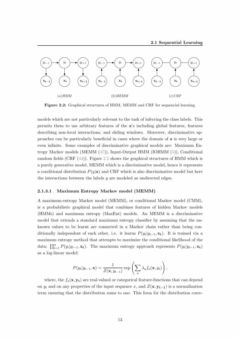
Figure 2.2: Graphical structures of HMM, MEMM and CRF for sequencial learning.
models which are not particularly relevant to the task of inferring the class labels. This
permits them to use arbitrary features of the x’s including global features, features
describing non-local interactions, and sliding windows. Moreover, discriminative ap-
proaches can be particularly beneficial in cases where the domain of x is very large or
even infinite. Some examples of discriminative graphical models are: Maximum En-
tropy Markov models (MEMM (47)), Input-Output HMM (IOHMM (5)), Conditional
random fields (CRF (44)). Figure 2.2 shows the graphical structures of HMM which is
a purely generative model, MEMM which is a discriminative model, hence it represents
a conditional distribution P (y|x) and CRF which is also discriminative model but here
the interactions between the labels y are modeled as undirected edges.
2.1.3.1 Maximum Entropy Markov model (MEMM)
A maximum-entropy Markov model (MEMM), or conditional Markov model (CMM),
is a probabilistic graphical model that combines features of hidden Markov models
(HMMs) and maximum entropy (MaxEnt) models. An MEMM is a discriminative
model that extends a standard maximum entropy classifier by assuming that the un-
known values to be learnt are connected in a Markov chain rather than being con-
ditionally independent of each other, i.e. it learns P (yt|yt−1,xt). It is trained via a
maximum entropy method that attempts to maximize the conditional likelihood of the
data:∏n
i=1 P (yi|yi−1,xt). The maximum entropy approach represents P (yt|yt−1,xt)
as a log-linear model:
P (yt|yt−1,x) =1
Z(x, yt−1)exp
(∑
a
λafa(x, yt)
)
,
where, the fa(x,yt) are real-valued or categorical feature-functions that can depend
on yt and on any properties of the input sequence x, and Z(x,yt−1) is a normalization
term ensuring that the distribution sums to one. This form for the distribution corre-
13
2. BACKGROUND
sponds to the maximum entropy probability distribution satisfying the constraint that
the empirical expectation for the feature is equal to the expectation given the model:
Ee [fa(x,y)] = Ep [fa(x,y)] ∀a.
The parameters λa can be estimated using generalized iterative scaling (21). The
optimal state sequence y1, . . . , yn can be found using a very similar Viterbi algorithm
to the one used for HMMs.
Bengio and Frasconi (5) introduced a variation of MEMM called Input-Output
HMM (IOHMM). It is similar to the MEMM except that it introduces hidden state
variables st in addition to the output labels yt. Sequential interactions are modeled by
the st variables. To handle these hidden variables during training, the Expectation-
Maximization (EM (22)) algorithm is applied.
One drawback of MEMMs and IOHMM models is that they potentially suffer from
the ”label bias problem”. Notice that in MEMM model:
∑
yt
P (yt|yt−1,x1, . . . ,xt) =∑
yt
P (yt|yt− 1,xt) · P (yt−1|x1, . . . ,xt−1)
= 1 · P (yt|yt−1,x1, . . . ,xt−1)
= P (yt|yt−1,x1, . . . ,xt−1)
This says that the total probability mass “received” by yt−1 (based on x1, . . . , xt−1)
must be “transmitted” to labels yt at time t regardless of the value of xt. The only
role of xt is to influence which of the labels receive more of the probability at time t.
In particular, all of the probability mass must be passed on to some yt even if xt is
completely incompatible with yt. Thus, observations xt from later in the sequence has
absolutely no effect on the posterior probability of the current state; or, in other words,
the model does not allow for any smoothing.
Conditional random fields (CRF) (44) were designed to overcome this weakness,
which had already been recognized in the context of neural network-based Markov
models in the early 1990s. Another source of label bias is that training is always done
with respect to known previous predictions, so the model struggles at test time when
there is uncertainty in the previous prediction.
2.1.3.2 Conditional Random Fields (CRF)
Conditional random fields (44) are a type of discriminative undirected probabilistic
graphical model. In the CRF, the relationship among adjacent pairs yt−1 and yt is
modeled as an Markov Random Field (13) conditioned on the x inputs. In other
14
2.1 Sequential Learning
words, the way in which the adjacent y values influence each other is determined by
the input features. It is used to encode known relationships between examples and
construct consistent interpretations. The CRF is represented by a set of potentials
Mt(yt−1, yt|x), for each position in t in the sample sequence x, it is defined as:
Mt(yt−1, yt|x) = exp(Λt(yt−1, yt|x))Λt(yt−1, yt|x) =
∑
k
λkfk(yt−1, yt,x) +∑
k
µkgk(yt,x),
where the fk are features that encode some information about yt−1, yt, and arbitrary
information about x, and the gk are features that encode some information about yt and
x. It is assumed that both fk and gk are given and fixed. In this way, it is possible to
incorporate arbitrarily long-distance information about x. The conditional probability
P (y|x) is written as:
P (y|x) =∏n+1
t=1 Mt(yt−1, yt|x)[∏n+1
t=1 Mt(x)]
start,stop
,
where y0 = start and yn+1 = stop. The normalizer in the denominator is needed
because the potentials Mt are unnormalized ”scores”.
The training of CRFs is expensive, because it requires a global adjustment of the
λ values. This global training is what allows the CRF to overcome the label bias
problem by allowing the xt values to modulate the relationships between adjacent yt−1
and yt values. Algorithms based on iterative scaling and gradient descent have been
developed for optimizing both P (y|x) and also for separately optimizing P (yt|x) for
loss functions that depend only on the individual label. Whereas in HMMs or MEEMs
case, each gradient step required only a single execution of inference, when training a
CRF, we must execute inference for every single data case, conditioning on variables x.
This makes the training phase considerably more expensive than HMMs or MEMMs.
For example, in image classification task, inference step using a generative method
involves summation over the space of all possible images; if we have N×N image where
each pixel can take 256 values, the resulting space has 256N2values, giving rise to a
highly intractable inference problem (even using approximate inference methods). The
next section shows other methods and approaches that particularly exploit contextual
information in image classification tasks.
15
2. BACKGROUND
2.2 Contextual information in image classification tasks
While the contribution of this thesis can appear limited into the machine learning area,
it is also of interest for the computer vision community. A large part of the com-
puter vision community is recently devoting efforts to exploit contextual information
to improve classification performance in object/class recognition and segmentation. For
these reasons, relevant state of the art comes from machine learning as well as from
computer vision communities.
The use of contextual information is potentially able to cope with ambiguous cases
in classification. Moreover, the contextual information can increase a machine learning
system performance both in terms of accuracy and precision, thus helping to reduce
both false positive and false negatives. However, the methods presented in the previous
section suffer from different disadvantages.
Although CRFs are a general and powerful framework for combining features and
contextual information, its application to image classification tasks can be very ex-
pensive. This is because the computational cost of both training and inference are
very high and both proportional to the exponential of the clique cardinality. Since we
assume that all the variables are observed in the training set, we can find the global
optimum of the objective function, so long as we can compute the gradient exactly.
Unfortunately for CRF involving large clique cardinality it is not tractable to compute
the exact gradient. Several approximate inference methods have been used, like mean
field, loopy belief propagation (69) or graph cuts (11). Even though approximate in-
ference methods will be used, if the clique is not reduced to a few nodes (usually the
4-neighborhood, i.e. the pixels at north, west, south and east of the center pixel), it is
infeasible to compute the inference step. In fact, successful CRF models (43, 68) have
been applied to groups of pixels using a clique of size 2 on a 4-neighborhood.
Other methods of the literature exploit contextual information by identifying super-
pixels using segmentation algorithms tuned to perform over-segmentation (18, 36, 37).
In (37), for example, the set of super-pixels is clustered forming a vocabulary of possible
local contexts. Finally, the super-pixels are considered as the context for classification
by considering the spatial relationship between the pixel (or area) being classified and
the neighborhood super-pixels. In (18, 36) the super-pixels are used to form the puzzle
that better fits the object, using also contextual information, and geometric coher-
ence, among different puzzles. All these methods assume that an over-segmentation
is possible, and hopefully, different super-pixels can cluster together in a semantically
meaningful way.
16
2.3 Sequential learning in multi-class problems
Other contextual methods extract a global representation of the context, and use
it to influence the classification step. In (65), the context is modeled globally. Thus,
the method does not locally compute the context and can not relate labels (or objects)
spatially (or temporally) by means of the local context.
2.3 Sequential learning in multi-class problems
Usually, the applications considered need classifiers that are able to deal with multiple
classes. However, in the case of sequential learning, few of the previous approaches
are able to deal with the multi-class case. One case of multi-class extension is the
CRF using graph-cut with alpha-expansion (11). Another approach is to decompose
the multi-class problem into a set of binary-class problems and combine them in some
way. In this sense, the Error-Correct Output Codes (ECOC) (24) framework is a well-
studied methodology that is used to transform multi-class problems to an ensemble
of binary classifiers. The fundamental issues here are: how this decomposition can be
done in an efficient way, and how a final classification can be obtained from the different
binary predictions. In the ECOC framework, these two issues are defined as coding and
decoding phases in a communication problem. During the coding phase a codeword is
assigned to each label in the multi-class problem. Each bit in the codeword identifies
the membership of such class for a given binary classifier. The most used coding
strategies are the one-versus-all (50), where each class is discriminated against the
rest and one-versus-one (3), which splits each possible pairs of classes. The decoding
phase of the ECOC framework is based on error-correcting principles, where distances
measurements between the output code and the target codeword are the strategies most
frequently applied. Among these, Hamming and Euclidean measures are the most used
(27).
2.4 Conclusions
Independently of the specific method, there are still fundamental issues in sequential
supervised learning that require the attention of the community. In (25) the authors
acknowledge the following issues: a) how to capture and exploit sequential correlations;
b) how to represent and incorporate complex loss functions; c) how to identify long-
distance interactions; d) how to make sequential learning computationally efficient.
In the next chapter we propose our contribution to the sequential learning research.
Our framework, called Generalized SSL (GSSL), is a generalization of the standard
17

2. BACKGROUND
stacked sequential learning stated in the stacked sequential learning section 2.1.1.2.
Our method aims to give an answer to these previous questions. Particularly, we are
interested in how to capture and exploit sequential correlations and how to identify
long-distance interactions, focusing on image classification tasks. Our secondary goal
is to do it as generally (i.e. setting the minimum number of parameter) as possible,
while being computationally efficient and accurate compared to general probabilisitics
models, as CRFs.
18
3
Generalized Stacked Sequential
Learning
In this chapter, first (Section 3.1) we propose a Generalized Stacked Sequential Learning
(GSSL) schema for classification tasks. As mentioned in the previous chapter, our
contribution is centered on sequential learning problems. Sequential learning assumes
that samples are not independently drawn from a joint distribution of the data samples
X and their labels Y . Therefore, here the training data is considered as a sequence of
pairs: example and its label (x, y), such that neighboring examples exhibit some kind
of relationship.
Cohen et al (17) presents an approach of sequential learning based on a meta-
learning framework (71) . Basically, the Stacked Sequential Learning (SSL) scheme is
a two layers classifier where, firstly, a base classifier H1(x) is trained and tested with
the original data X. Then, an extended data set is created which joins the original
training data features X with the predicted labels Y ′ produced by the base classifier
considering a fixed-size window around the example. Finally, second classifier H2(x)
is trained with this new feature set. The final result is a set of predictions Y . Figure
3.1 shows a scheme of the SSL framework. As said before, the main drawback of
this SSL approach is that the width of the window around the sample determines the
maximum length of interaction among samples. Therefore, the longer the window,
the further the interaction is considered, but also the extended data set is increased in
terms of features. This makes this approach not suitable for problems that present long
range sequential relationships. Furthermore, if we consider more than one relationship
dimension, the size of the extended set increases exponentially, making it not feasible
for sequential types of datasets like images, videos, or time series. Our method aims to
19
3. GENERALIZED STACKED SEQUENTIAL LEARNING
give an answer to these drawbacks. Particularly, we are interested in how to capture and
exploit sequential correlations and how to identify long-distance interactions, focusing
on image classification tasks. Our secondary goal is to do it as generally (i.e. setting
the minimum number of parameter) as possible, while being computationally efficient
and accurate compared with general probabilisitics models, as CRFs.
Next, section 3.2 describes our implementation of Generalized Stacked Sequential
Learning, called Multi-scale Stacked Sequential Learning (MSSL), which gives response
to these questions. Finally this chapter ends (Section 3.3) with some experiments using
our approach and a discussion of the results obtained.
H1(x) ∪ H2(x)
X
Y′
X
X′ = (X;Y ′) Y
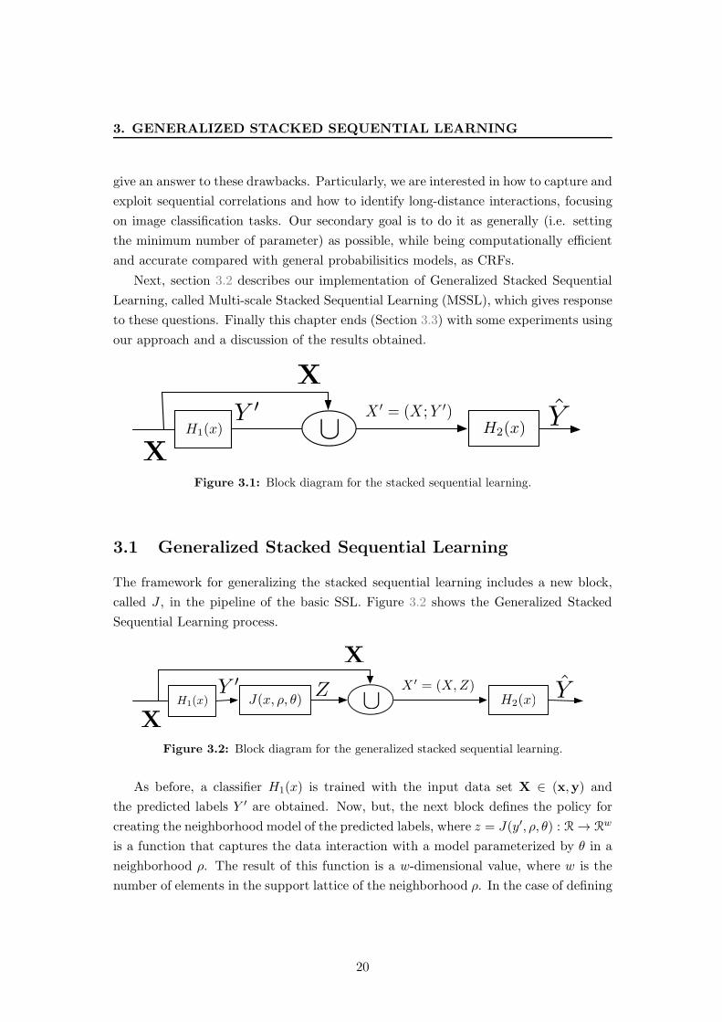
Figure 3.1: Block diagram for the stacked sequential learning.
3.1 Generalized Stacked Sequential Learning
The framework for generalizing the stacked sequential learning includes a new block,
called J , in the pipeline of the basic SSL. Figure 3.2 shows the Generalized Stacked
Sequential Learning process.
H1(x) J(x, ρ, θ) ∪ H2(x)
X
Y′
Z
X
X′ = (X,Z) Y
Figure 3.2: Block diagram for the generalized stacked sequential learning.
As before, a classifier H1(x) is trained with the input data set X ∈ (x,y) and
the predicted labels Y ′ are obtained. Now, but, the next block defines the policy for
creating the neighborhood model of the predicted labels, where z = J(y′, ρ, θ) : R→ Rw
is a function that captures the data interaction with a model parameterized by θ in a
neighborhood ρ. The result of this function is a w-dimensional value, where w is the
number of elements in the support lattice of the neighborhood ρ. In the case of defining
20
3.2 Multi-Scale Stacked Sequential Learning (MSSL)
MULTI-SCALE
DECOMPOSITION
SAMPLING
PATTERN
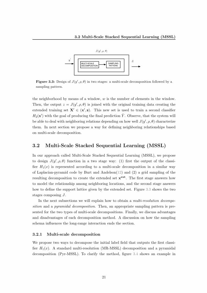
z
Figure 3.3: Design of J(y′, ρ, θ) in two stages: a multi-scale decomposition followed by a
sampling pattern.
the neighborhood by means of a window, w is the number of elements in the window.
Then, the output z = J(y′, ρ, θ) is joined with the original training data creating the
extended training set X′ ∈ (x′, z). This new set is used to train a second classifier
H2(x′) with the goal of producing the final prediction Y . Observe, that the system will
be able to deal with neighboring relations depending on how well J(y′, ρ, θ) characterize
them. In next section we propose a way for defining neighboring relationships based
on multi-scale decomposition.
3.2 Multi-Scale Stacked Sequential Learning (MSSL)
In our approach called Multi-Scale Stacked Sequential Learning (MSSL), we propose
to design J(y′, ρ, θ) function in a two stage way: (1) first the output of the classi-
fier H1(x) is represented according to a multi-scale decomposition in a similar way
of Laplacian-pyramid code by Burt and Andelson(12) and (2) a grid sampling of the
resulting decomposition to create the extended set xext. The first stage answers how
to model the relationship among neighboring locations, and the second stage answers
how to define the support lattice given by the extended set. Figure 3.3 shows the two
stages composing J .
In the next subsections we will explain how to obtain a multi-resolution decompo-
sition and a pyramidal decomposition. Then, an appropriate sampling pattern is pre-
sented for the two types of multi-scale decompositions. Finally, we discuss advantages
and disadvantages of each decomposition method. A discussion on how the sampling
schema influences the long-range interaction ends the section.
3.2.1 Multi-scale decomposition
We propose two ways to decompose the initial label field that outputs the first classi-
fier H1(x). A standard multi-resolution (MR-MSSL) decomposition and a pyramidal
decomposition (Pyr-MSSL). To clarify the method, figure 3.4 shows an example in
21
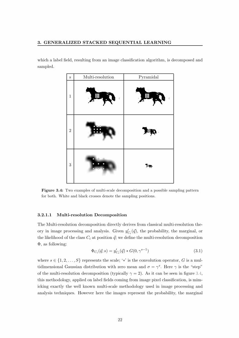
3. GENERALIZED STACKED SEQUENTIAL LEARNING
which a label field, resulting from an image classification algorithm, is decomposed and
sampled.
s Multi-resolution Pyramidal
1
2
3
Figure 3.4: Two examples of multi-scale decomposition and a possible sampling pattern
for both. White and black crosses denote the sampling positions.
3.2.1.1 Multi-resolution Decomposition
The Multi-resolution decomposition directly derives from classical multi-resolution the-
ory in image processing and analysis. Given y′Ci(~q), the probability, the marginal, or
the likelihood of the class Ci at position ~q; we define the multi-resolution decomposition
Φ, as following:
ΦCi(~q; s) = y′Ci
(~q) ∗G(0, γs−1) (3.1)
where s ∈ {1, 2, . . . , S} represents the scale; ‘∗’ is the convolution operator, G is a mul-
tidimensional Gaussian distribution with zero mean and σ = γs. Here γ is the “step”
of the multi-resolution decomposition (typically γ = 2). As it can be seen in figure 3.4,
this methodology, applied on label fields coming from image pixel classification, is mim-
icking exactly the well known multi-scale methodology used in image processing and
analysis techniques. However here the images represent the probability, the marginal
22
3.2 Multi-Scale Stacked Sequential Learning (MSSL)
or the likelihood of a certain class. As a result, the Multi-resolution decomposition
provides information regarding the spatial homogeneity and regularity of the label field
at different scale. It is easy to understand that, for example, a noisy classification at
scale 1 does not influences importantly the results of scale 3. In this way, the highest
scale robustly represents the label field in presence of noisy classification (reaching the
limit of an almost homogeneous label field) and, at the same time, intermediate scales
give different levels of details in the initial label field.
3.2.1.2 Pyramidal Decomposition
An alternative is provided by the pyramidal decomposition (2). The pyramidal de-
composition is substantially similar to the multi-resolution decomposition with the
exception that actually, the resulting pyramid codify more efficiently the multi-scale
information. However, it has an important drawback that will be discussed in next
subsections.
Starting from the above mentioned Multi-resolution decomposition, the Pyramidal
decomposition Ψ can be obtained as follows:
ΨCi(~q; s) = ΦCi
(⌊kss~q⌋; s) (3.2)
where ⌊·⌋ is the floor function, ~q ∈ NN , N is the dimensionality of the data. Here
~qj ∈[
1Xj
γs−1
]
, where Xj is the integer size of every dimension j (for an image, N = 2,
X1 and X2 are respectively the width and height of the image). Here ks is the sampling
step and depends on γ, ks = γs/2. Actually, the pyramidal decomposition samples the
Multi-resolution theoretically without loss of information, since at higher scales, the
high frequency content have been progressively filtered out.
3.2.1.3 Pros and cons of multi-resolution and pyramidal decompositions
The multi-resolution approach is the most appropriate in terms of signal processing
theory. However, the pyramidal decomposition actually contains the same information
as the multi-resolution while coding it in a more compact way. Unfortunately, as it can
be noticed in formula (3.5), the sampling at large scales is prone to produce blocking
artifacts. This is due to the fact that during the pyramidal decomposition process,
each scale summarizes the information of the above area in a block that is γN times
smaller (here N is the dimensionality of the data, for images N = 2). Obviously, at
large scales this reflects a sharp transition form a value to another in the feature vector.
This does not happen using the multi-resolution decomposition, where the Gaussian
filtering assures smooth transitions at every scale.
23
3. GENERALIZED STACKED SEQUENTIAL LEARNING
Summarizing, if the input data is sufficiently small, the use of the multi-resolution
decomposition is highly recommended, while if the input data is inherently large, the
pyramidal decomposition can help to save memory at the cost of possible blocking
artifacts. To avoid blocking artifacts, an interpolation technique could be used. How-
ever, after the next step, sampling pattern, the resulting output will be the same size,
therefore pyramidal decomposition compactness is not a big advantage. For sake of
simplicity, our MSSL framework will use the multi-resolution approach as a standard
multi-scale decomposition method.
3.2.2 Sampling pattern
Once the desired multi-scale representation has been computed, an appropriate sam-
pling pattern should be applied. This pattern can be represented by a set of displace-
ment vectors that defines the neighborhood ρ =⋃M
m=1~δm. Once the displacement vec-
tors are defined, the feature vector for the multi-resolution decomposition is obtained
by the following formula:
z(~p) = {Φ(~p + ~δ1; 1),Φ(~p + ~δ2; 1), . . . ,Φ(~p+ ~δM ; 1),︸ ︷︷ ︸
scale s=1
Φ(~p+ γ ~δ1; 2),Φ(~p + γ ~δ2; 2), . . . ,Φ(~p+ γ ~δM ; 2),︸ ︷︷ ︸
scale s=2
...
Φ(~p+ γ(S−1) ~δ1;S),Φ(~p + γ(S−1) ~δ2;S), . . . ,Φ(~p+ γ(S−1) ~δM ;S)︸ ︷︷ ︸
scale s=S
}
(3.3)
This formula shows that the sampling is performed following the displacement vectors
at each scale s. However, the displacement at different scales are multiplied by a factor
γ(s−1) so that, higher scales correspond to larger displacement. For the sake of clarity,
the sampling in figure 3.4 (left) is obtained with S = 3, γ = 2, M = 9 and the following
set of displacements:
ρ = { ~δ1 = (−1,−1), ~δ2 = (−1, 0), ~δ3 = (−1, 1),~δ4 = (0,−1), ~δ5 = (0, 0), ~δ6 = (0, 1),~δ7 = (1,−1), ~δ8 = (1, 0), ~δ9 = (1, 1)}.
(3.4)
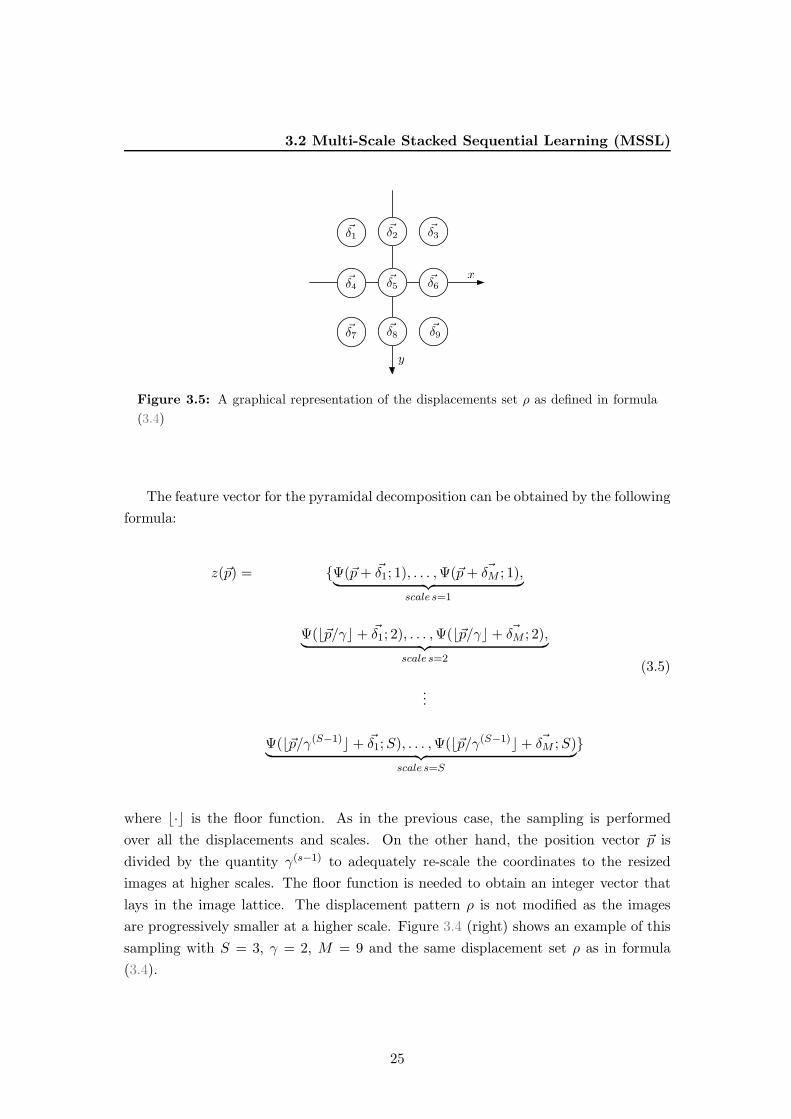
This displacement set can be represented graphically as in figure 3.5.
24
3.2 Multi-Scale Stacked Sequential Learning (MSSL)
!δ1
!δ2 !δ3
!δ4
!δ5 !δ6
!δ7
!δ8 !δ9
x
y
Figure 3.5: A graphical representation of the displacements set ρ as defined in formula
(3.4)
The feature vector for the pyramidal decomposition can be obtained by the following
formula:
z(~p) = {Ψ(~p+ ~δ1; 1), . . . ,Ψ(~p+ ~δM ; 1),︸ ︷︷ ︸
scale s=1
Ψ(⌊~p/γ⌋+ ~δ1; 2), . . . ,Ψ(⌊~p/γ⌋ + ~δM ; 2),︸ ︷︷ ︸
scale s=2
...
Ψ(⌊~p/γ(S−1)⌋+ ~δ1;S), . . . ,Ψ(⌊~p/γ(S−1)⌋+ ~δM ;S)︸ ︷︷ ︸
scale s=S
}
(3.5)
where ⌊·⌋ is the floor function. As in the previous case, the sampling is performed
over all the displacements and scales. On the other hand, the position vector ~p is
divided by the quantity γ(s−1) to adequately re-scale the coordinates to the resized
images at higher scales. The floor function is needed to obtain an integer vector that
lays in the image lattice. The displacement pattern ρ is not modified as the images
are progressively smaller at a higher scale. Figure 3.4 (right) shows an example of this
sampling with S = 3, γ = 2, M = 9 and the same displacement set ρ as in formula
(3.4).
25
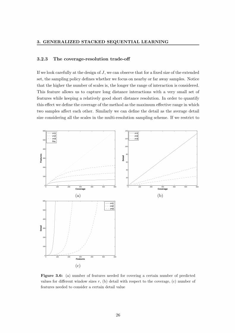
3. GENERALIZED STACKED SEQUENTIAL LEARNING
3.2.3 The coverage-resolution trade-off
If we look carefully at the design of J , we can observe that for a fixed size of the extended
set, the sampling policy defines whether we focus on nearby or far away samples. Notice
that the higher the number of scales is, the longer the range of interaction is considered.
This feature allows us to capture long distance interactions with a very small set of
features while keeping a relatively good short distance resolution. In order to quantify
this effect we define the coverage of the method as the maximum effective range in which
two samples affect each other. Similarly we can define the detail as the average detail
size considering all the scales in the multi-resolution sampling scheme. If we restrict to
0 100 200 300 400 500 6000
100
200
300
400
500
600
Coverage
Fea
ture
s
r=1r=2r=3f=c
0 100 200 300 400 500 6000
20
40
60
80
100
120
140
Coverage
Det
ail
r=1r=2r=3
(a) (b)
0 100 200 300 400 500 6000
100
200
300
400
500
600
Features
Det
ail
r=1r=2r=3
(c)
Figure 3.6: (a) number of features needed for covering a certain number of predicted
values for different window sizes r, (b) detail with respect to the coverage, (c) number of
features needed to consider a certain detail value
26

3.3 Experiments and Results
grid square samplings, the sampling scheme can be expressed as a set of displacements
obtained by ~δ = (k · i, k · j) where i, j ∈ {1, 0,−1} and k = 1, 2, . . . , r. This defines a
square grid of size 2r + 1 centered at the sample of interest as the one shown in figure
3.5. The value of r plays an important role in the scheme since it allows to govern
the average detail of the approximation. In this setup the coverage can be computed
as c = γ(S−1)(2r + 1)d, the number of features generated by the proposed approach is
f = S(2r + 1)d and detail is computed as the average value of the relative distance
between adjacent points at scale i, given by γi−1. Thus, d = 1S
∑S−1i=0 γi = γS−1
γ−1 .
Figure 3.6 shows the relationship among detail, coverage and number of features.
Figure 3.6(a) plots the number of features needed for observing a certain number of
predicted labels (coverage). Different curves show the effect of altering the size of
the support window r. Thus, in a 2-dimensional sequential domain if the support
window has a size of 3, r = 1, we need 7 scales and a total of 63 features to capture
information from about 600 labels. The parameter r governs the trade-off between
resolution and coverage. Observe in Figure 3.6(b) that average detail is coarser as the
coverage increases. Thus, small patterns in long distance label interactions are lost. As
r increases, the number of features also increase (Figure 3.6(c)), but more complex and
detailed label patterns can be captured. On the contrary, maximum interaction details
are observed at the cost of using the same number of features as the coverage value.
This trade-off allows the practitioner to consider different strategies according to the
degree of sequential correlation expected in the sequence.
3.3 Experiments and Results
In order to validate the proposed techniques, MR-SSL and Pyr-SSL are applied and
compared to state-of-the-art strategies in two different scenarios. The first scenario
considers one dimensional correlations in the label field in a text categorization task.
The second experiment concerns the image domain, where correlations are found on a
two dimensional support lattice.
3.3.1 Categorization of FAQ documents
• Dataset The FAQ categorization task has been frequently used in literature as a
benchmark for sequential learners (17) (26). In this data set, three different com-
puter science FAQ groups pages are used (ai-neural-nets, ai-general, aix). Each
FAQ group consists of 5 to 7 long sequences of lines; each sequence corresponds to
a single FAQ document. Each line is characterized using McCallun et al features
27
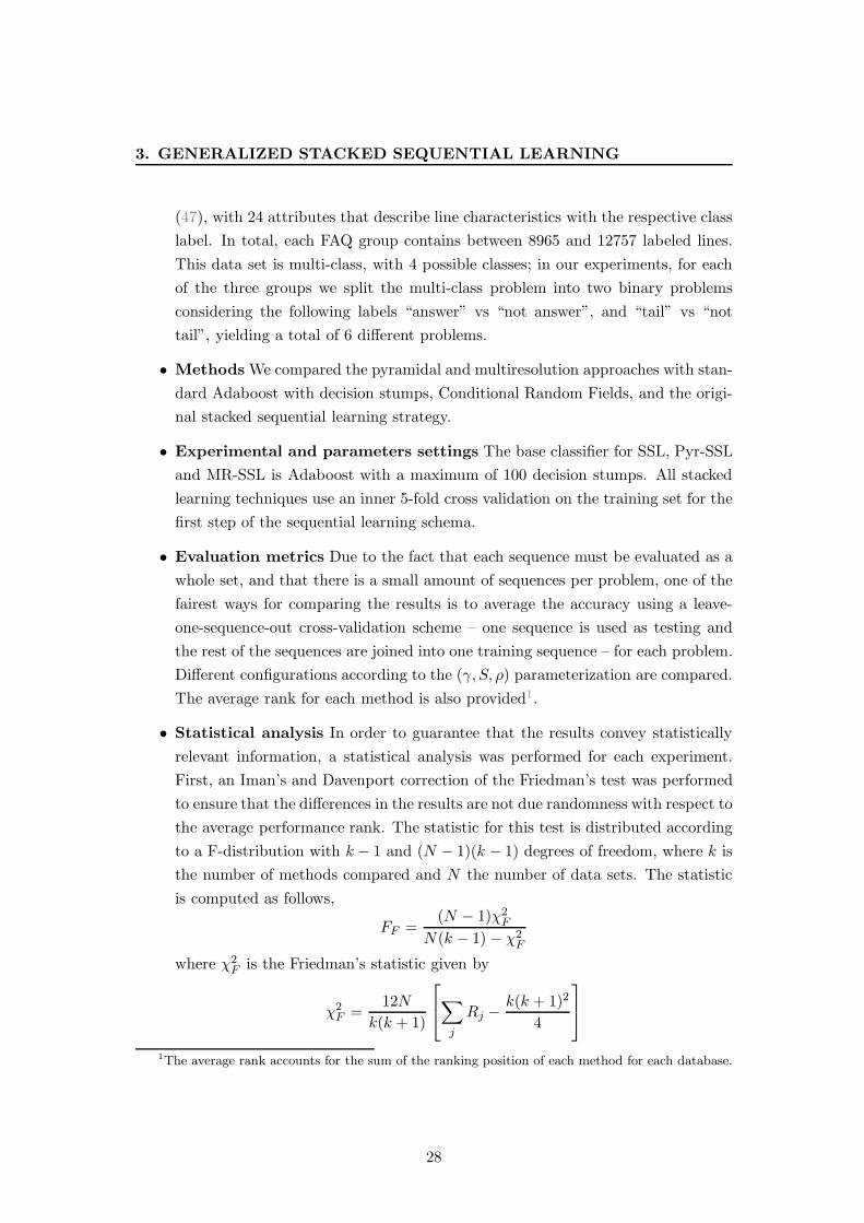
3. GENERALIZED STACKED SEQUENTIAL LEARNING
(47), with 24 attributes that describe line characteristics with the respective class
label. In total, each FAQ group contains between 8965 and 12757 labeled lines.
This data set is multi-class, with 4 possible classes; in our experiments, for each
of the three groups we split the multi-class problem into two binary problems
considering the following labels “answer” vs “not answer”, and “tail” vs “not
tail”, yielding a total of 6 different problems.
• Methods We compared the pyramidal and multiresolution approaches with stan-
dard Adaboost with decision stumps, Conditional Random Fields, and the origi-
nal stacked sequential learning strategy.
• Experimental and parameters settings The base classifier for SSL, Pyr-SSL
and MR-SSL is Adaboost with a maximum of 100 decision stumps. All stacked
learning techniques use an inner 5-fold cross validation on the training set for the
first step of the sequential learning schema.
• Evaluation metrics Due to the fact that each sequence must be evaluated as a
whole set, and that there is a small amount of sequences per problem, one of the
fairest ways for comparing the results is to average the accuracy using a leave-
one-sequence-out cross-validation scheme – one sequence is used as testing and
the rest of the sequences are joined into one training sequence – for each problem.
Different configurations according to the (γ, S, ρ) parameterization are compared.
The average rank for each method is also provided1.
• Statistical analysis In order to guarantee that the results convey statistically
relevant information, a statistical analysis was performed for each experiment.
First, an Iman’s and Davenport correction of the Friedman’s test was performed
to ensure that the differences in the results are not due randomness with respect to
the average performance rank. The statistic for this test is distributed according
to a F-distribution with k − 1 and (N − 1)(k − 1) degrees of freedom, where k is
the number of methods compared and N the number of data sets. The statistic
is computed as follows,
FF =(N − 1)χ2
F
N(k − 1)− χ2F
where χ2F is the Friedman’s statistic given by
χ2F =
12N
k(k + 1)
∑
j
Rj −k(k + 1)2
4
1The average rank accounts for the sum of the ranking position of each method for each database.
28
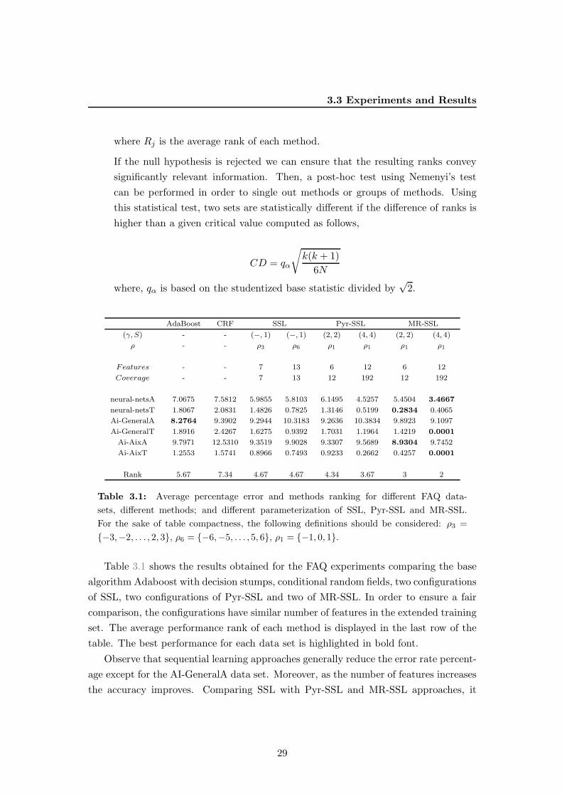
3.3 Experiments and Results
where Rj is the average rank of each method.
If the null hypothesis is rejected we can ensure that the resulting ranks convey
significantly relevant information. Then, a post-hoc test using Nemenyi’s test
can be performed in order to single out methods or groups of methods. Using
this statistical test, two sets are statistically different if the difference of ranks is
higher than a given critical value computed as follows,
CD = qα
√
k(k + 1)
6N
where, qα is based on the studentized base statistic divided by√2.
AdaBoost CRF SSL Pyr-SSL MR-SSL
(γ, S) - - (−, 1) (−, 1) (2, 2) (4, 4) (2, 2) (4, 4)
ρ - - ρ3 ρ6 ρ1 ρ1 ρ1 ρ1
Features - - 7 13 6 12 6 12
Coverage - - 7 13 12 192 12 192
neural-netsA 7.0675 7.5812 5.9855 5.8103 6.1495 4.5257 5.4504 3.4667
neural-netsT 1.8067 2.0831 1.4826 0.7825 1.3146 0.5199 0.2834 0.4065
Ai-GeneralA 8.2764 9.3902 9.2944 10.3183 9.2636 10.3834 9.8923 9.1097
Ai-GeneralT 1.8916 2.4267 1.6275 0.9392 1.7031 1.1964 1.4219 0.0001
Ai-AixA 9.7971 12.5310 9.3519 9.9028 9.3307 9.5689 8.9304 9.7452
Ai-AixT 1.2553 1.5741 0.8966 0.7493 0.9233 0.2662 0.4257 0.0001
Rank 5.67 7.34 4.67 4.67 4.34 3.67 3 2
Table 3.1: Average percentage error and methods ranking for different FAQ data-
sets, different methods; and different parameterization of SSL, Pyr-SSL and MR-SSL.
For the sake of table compactness, the following definitions should be considered: ρ3 =
{−3,−2, . . . , 2, 3}, ρ6 = {−6,−5, . . . , 5, 6}, ρ1 = {−1, 0, 1}.
Table 3.1 shows the results obtained for the FAQ experiments comparing the base
algorithm Adaboost with decision stumps, conditional random fields, two configurations
of SSL, two configurations of Pyr-SSL and two of MR-SSL. In order to ensure a fair
comparison, the configurations have similar number of features in the extended training
set. The average performance rank of each method is displayed in the last row of the
table. The best performance for each data set is highlighted in bold font.
Observe that sequential learning approaches generally reduce the error rate percent-
age except for the AI-GeneralA data set. Moreover, as the number of features increases
the accuracy improves. Comparing SSL with Pyr-SSL and MR-SSL approaches, it
29
3. GENERALIZED STACKED SEQUENTIAL LEARNING
Pyr-SSL MR-SSL
(γ, S) (2, 2) (2, 3) (2, 4) (4, 4) (2, 2) (2, 3) (2, 4) (4, 4)
ρ ρ1 ρ1 ρ1 ρ1 ρ1 ρ1 ρ1 ρ1
Features 6 9 12 12 6 9 12 12
Coverage 12 24 48 192 12 24 48 192
neural-netsA 6.1495 5.624 4.9195 4.5257 5.4504 4.6303 4.0018 3.4667
neural-netsT 1.3146 0.7159 0.5257 0.5199 0.2834 0.2499 0.2210 0.4065
Ai-GeneralA 9.2636 9.1998 9.0374 10.3834 9.8923 9.3698 8.8874 9.1097
Ai-GeneralT 1.7031 1.2716 0.6582 1.1964 1.4219 0.7136 0.6407 0.0001
Ai-AixA 9.3307 9.3412 9.1311 9.5689 8.9304 9.1276 9.2907 9.7452
Ai-AixT 0.9233 0.4754 0.2888 0.2662 0.4257 0.0001 0.0806 0.0001
Rank 7 6.17 4 5.33 5 3.25 2.16 3.08
Avg rank 5.63 3.37
Table 3.2: Average percentage error for different configurations of Pyr-SSL and MR-SSL.
The last two rows show the average rank for each parameterization as well as the average
rank for each of the multi-scale families.
is worth noting that using a similar number of features, the multi-scale counterparts
achieve much better results. This seems to suggest that the data sets include some
structure information that can only be captured at large scales. This idea is reinforced
by the fact that for some of the data sets, the larger the coverage, the lower the error
rate achieved. Finally, when the multi-scale step γ is doubled – thus quadrupling the
coverage by sacrificing resolution in the data sequence – we can see that applying Pyr-
SSL accuracy improves on half of the data sets. On the other hand, when applying
MR-SSL accuracy improves in all except for one data set.
Observing the ranks for all proposed methods, it can be noticed that Pyr-SSL
and MR-SSL strategies perform better than Adaboost, CRF and SSL. Considering the
different configurations of the MSSL technique, Pyr-SSL performs poorer than MR-
SSL. A detailed analysis of this effect is shown in Table 3.2.
A statistical analysis of the results shows that, in our case, Iman’s and Davenport
correction of the Friedman’s test yields FF = 2.9329 and the critical value for this test
is F (7, 35) = 2.249, so we reject the null hypothesis that the results may be due to
randomness with respect to the average rank. Thus we can safely say that the analysis
of ranks convey statistically relevant information.
A post-hoc analysis of the data using Nemenyi’s test1 singles out MR-SSL (4, 4) from
SSL, CRF and AdaBoost with a 95% confidence. Additionally, all proposed strategies
1Critical difference using Nemenyi’s test at 0.05 is 2.44, and at 0.10 is 2.05.
30
3.3 Experiments and Results
are statistically different than CRF and Adaboost at 90% confidence. On the other
hand, SSL shows statistically significant differences with respect to CRF, as reported
in the original SSL paper but fails to display any statistically significative difference
with respect to Adaboost.
Table 3.2 shows a detailed comparison between Pyr-SSL and MR-SSL using different
parameter configurations. Average ranks for each configuration are provided. Addi-
tionally, a single average rank for Pyr-MSSL and MR-SSL is given. The parameters
are chosen such that the number of features and coverages are comparable.
Using Iman’s and Davenport statistic FF = 6.0689, with a critical value for F (7, 35) =
2.249, so we reject the null hypothesis that the results may be due to randomness with
respect to the average rank. A post-hoc test using Nemenyi’s test critical difference
with 95% of confidence shows that MR-SSL always statistically outperforms Pyr-SSL
when we compare the same parameter configurations.
3.3.2 Weizmann horse database
• Dataset The Weizmann horse database is composed of 328 side-view color images
of horses and their respective manual segmentations. This database has been
proposed to evaluate the performance of a segmentation algorithm (7). In the
database, the horses exhibit a sufficiently regular structure; i.e. all are standing
and face towards the left. They vary significantly in color and size.
• Methods We compared the proposed methods against AdaBoost, CRF and stan-
dard SSL (using a window of size 7×7). For the following experiments, the CRF
implementation is a modified version of the one in (68). We incorporated Ad-
aBoost to generate the unary potential. In this way, the base classifier for all the
SSL strategies is the same as the one used by CRF. For the learning phase we used
the stochastic gradient descent as it proved to be one of the fastest ways to train
a CRF (68). Finally, inference is performed by means of the belief propagation
method.
• Experimental and parameters settings
Two different experiments are performed using this dataset:
– First, in order to perform a fair comparison to the method in (7), we resize
all the images to 40x30 pixel size. This problem will also serve to establish
proper comparisons with computationally intensive methods such as CRF.
31
3. GENERALIZED STACKED SEQUENTIAL LEARNING
A good way to show the capabilities of the proposed method, is to reduce
the number of features that the first classifier can use to discriminate the
horse class. In this way, the behavior of the proposed method will be easier
to describe. We actually reduce the feature vector to pixel-wise color. The
images are transformed from sRGB to CIELAB color space to highlight
lightness and chromatic components. The first classifier (h1(x)) only has
access to the three CIELAB color coordinates for each pixel in the image.
Observe that this classification can be prone to several errors due to the
similarity between horses color and background color. Moreover, since the
classification is performed pixel-wise, the first classifier is prone to isolated
misclassifications.
As in the previous experiment, the base classifier is an AdaBoost with deci-
sion stumps reaching a maximum of 100 iterations. Regarding the MR-SSL,
to have an effective long-range label interaction, we set the number of scales
S = 5, γ = 2 and ρ as in formula (3.4), so that the maximum displacement
during sampling is of ±γ(S−1) = ±24 = ±16 pixel, thus covering great part
of the image size.
– In order to show that the proposed method also works well with bigger
images, the other experiment uses full size images. In this case results are
compared with segmentation state-of-the-art methods.
To deal with full size images, we use the SIFT descriptor for the first classifier
(using the CIELAB color space) because texture is an important feature
when the images have a sufficient resolution. Moreover, we set the number
of scales S = 7, γ = 2 and ρ as in formula (3.4), obtaining a coverage value
of ±64 pixels.
• Evaluation metrics
Due to the significant amount of data a 5-fold cross-validation technique is used
for obtaining the average evaluation metrics. As done in (7), we used the Jac-
card index (40) as a quality measure of the overlapping o between the automatic
segmentation and the labeled ground-truth; being A and M respectively the au-
tomatic and manual (ground-truth) segmentations, the overlapping is defined as
o = |A∩M ||A∪M | . This measure is equivalent to the ratio of the true positive over the
sum of true positive, false positive and false negatives.
• Statistical analysis The amount of data in these experiments enable the pos-
sibility of using powerful statistical tests that were not available in the former
32
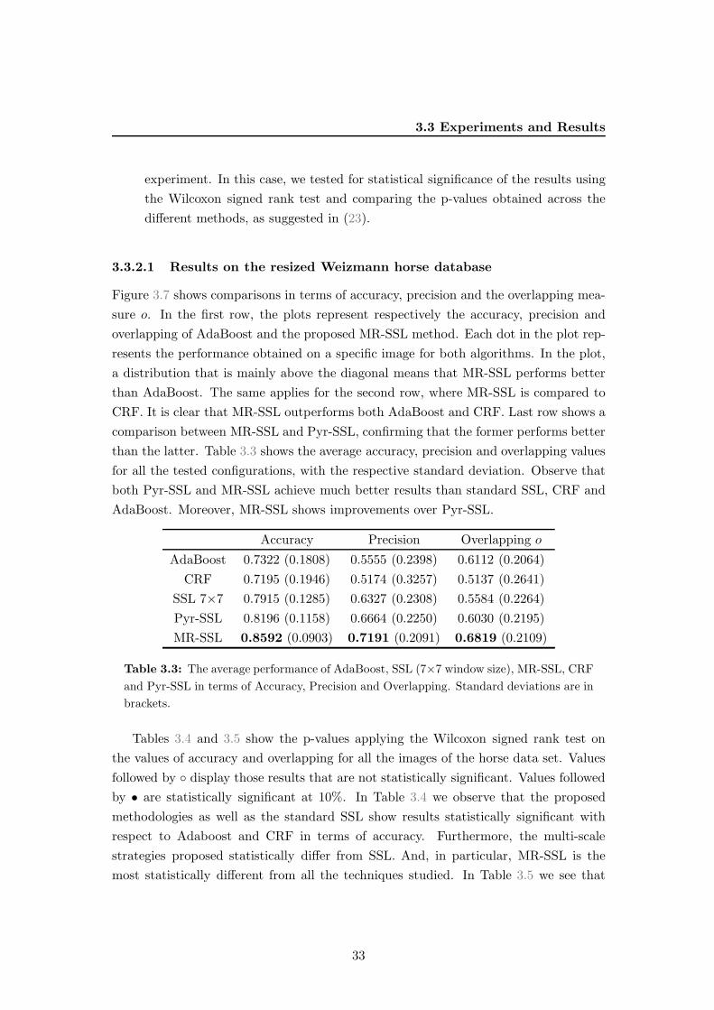
3.3 Experiments and Results
experiment. In this case, we tested for statistical significance of the results using
the Wilcoxon signed rank test and comparing the p-values obtained across the
different methods, as suggested in (23).
3.3.2.1 Results on the resized Weizmann horse database
Figure 3.7 shows comparisons in terms of accuracy, precision and the overlapping mea-
sure o. In the first row, the plots represent respectively the accuracy, precision and
overlapping of AdaBoost and the proposed MR-SSL method. Each dot in the plot rep-
resents the performance obtained on a specific image for both algorithms. In the plot,
a distribution that is mainly above the diagonal means that MR-SSL performs better
than AdaBoost. The same applies for the second row, where MR-SSL is compared to
CRF. It is clear that MR-SSL outperforms both AdaBoost and CRF. Last row shows a
comparison between MR-SSL and Pyr-SSL, confirming that the former performs better
than the latter. Table 3.3 shows the average accuracy, precision and overlapping values
for all the tested configurations, with the respective standard deviation. Observe that
both Pyr-SSL and MR-SSL achieve much better results than standard SSL, CRF and
AdaBoost. Moreover, MR-SSL shows improvements over Pyr-SSL.
Accuracy Precision Overlapping o
AdaBoost 0.7322 (0.1808) 0.5555 (0.2398) 0.6112 (0.2064)
CRF 0.7195 (0.1946) 0.5174 (0.3257) 0.5137 (0.2641)
SSL 7×7 0.7915 (0.1285) 0.6327 (0.2308) 0.5584 (0.2264)
Pyr-SSL 0.8196 (0.1158) 0.6664 (0.2250) 0.6030 (0.2195)
MR-SSL 0.8592 (0.0903) 0.7191 (0.2091) 0.6819 (0.2109)
Table 3.3: The average performance of AdaBoost, SSL (7×7 window size), MR-SSL, CRF
and Pyr-SSL in terms of Accuracy, Precision and Overlapping. Standard deviations are in
brackets.
Tables 3.4 and 3.5 show the p-values applying the Wilcoxon signed rank test on
the values of accuracy and overlapping for all the images of the horse data set. Values
followed by ◦ display those results that are not statistically significant. Values followed
by • are statistically significant at 10%. In Table 3.4 we observe that the proposed
methodologies as well as the standard SSL show results statistically significant with
respect to Adaboost and CRF in terms of accuracy. Furthermore, the multi-scale
strategies proposed statistically differ from SSL. And, in particular, MR-SSL is the
most statistically different from all the techniques studied. In Table 3.5 we see that
33
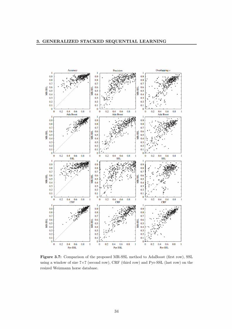
3. GENERALIZED STACKED SEQUENTIAL LEARNING
Figure 3.7: Comparison of the proposed MR-SSL method to AdaBoost (first row), SSL
using a window of size 7×7 (second row), CRF (third row) and Pyr-SSL (last row) on the
resized Weizmann horse database.
34
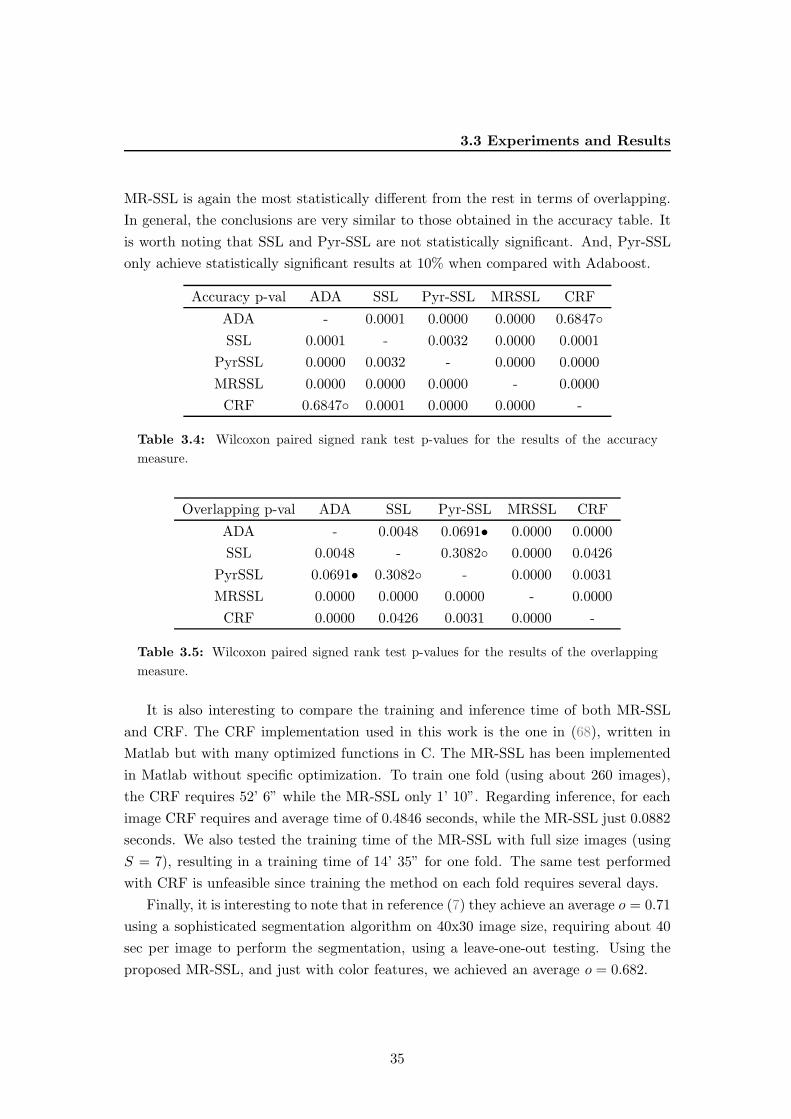
3.3 Experiments and Results
MR-SSL is again the most statistically different from the rest in terms of overlapping.
In general, the conclusions are very similar to those obtained in the accuracy table. It
is worth noting that SSL and Pyr-SSL are not statistically significant. And, Pyr-SSL
only achieve statistically significant results at 10% when compared with Adaboost.
Accuracy p-val ADA SSL Pyr-SSL MRSSL CRF
ADA - 0.0001 0.0000 0.0000 0.6847◦SSL 0.0001 - 0.0032 0.0000 0.0001
PyrSSL 0.0000 0.0032 - 0.0000 0.0000
MRSSL 0.0000 0.0000 0.0000 - 0.0000
CRF 0.6847◦ 0.0001 0.0000 0.0000 -
Table 3.4: Wilcoxon paired signed rank test p-values for the results of the accuracy
measure.
Overlapping p-val ADA SSL Pyr-SSL MRSSL CRF
ADA - 0.0048 0.0691• 0.0000 0.0000
SSL 0.0048 - 0.3082◦ 0.0000 0.0426
PyrSSL 0.0691• 0.3082◦ - 0.0000 0.0031
MRSSL 0.0000 0.0000 0.0000 - 0.0000
CRF 0.0000 0.0426 0.0031 0.0000 -
Table 3.5: Wilcoxon paired signed rank test p-values for the results of the overlapping
measure.
It is also interesting to compare the training and inference time of both MR-SSL
and CRF. The CRF implementation used in this work is the one in (68), written in
Matlab but with many optimized functions in C. The MR-SSL has been implemented
in Matlab without specific optimization. To train one fold (using about 260 images),
the CRF requires 52’ 6” while the MR-SSL only 1’ 10”. Regarding inference, for each
image CRF requires and average time of 0.4846 seconds, while the MR-SSL just 0.0882
seconds. We also tested the training time of the MR-SSL with full size images (using
S = 7), resulting in a training time of 14’ 35” for one fold. The same test performed
with CRF is unfeasible since training the method on each fold requires several days.
Finally, it is interesting to note that in reference (7) they achieve an average o = 0.71
using a sophisticated segmentation algorithm on 40x30 image size, requiring about 40
sec per image to perform the segmentation, using a leave-one-out testing. Using the
proposed MR-SSL, and just with color features, we achieved an average o = 0.682.
35
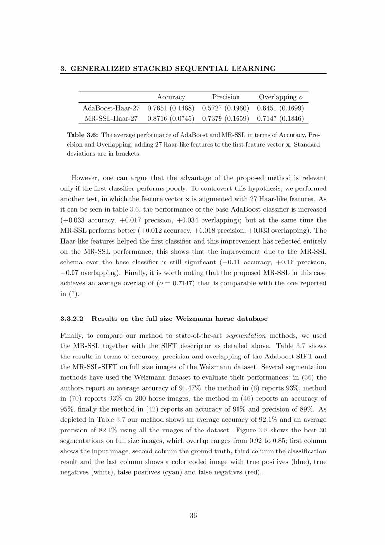
3. GENERALIZED STACKED SEQUENTIAL LEARNING
Accuracy Precision Overlapping o
AdaBoost-Haar-27 0.7651 (0.1468) 0.5727 (0.1960) 0.6451 (0.1699)
MR-SSL-Haar-27 0.8716 (0.0745) 0.7379 (0.1659) 0.7147 (0.1846)
Table 3.6: The average performance of AdaBoost and MR-SSL in terms of Accuracy, Pre-
cision and Overlapping; adding 27 Haar-like features to the first feature vector x. Standard
deviations are in brackets.
However, one can argue that the advantage of the proposed method is relevant
only if the first classifier performs poorly. To controvert this hypothesis, we performed
another test, in which the feature vector x is augmented with 27 Haar-like features. As
it can be seen in table 3.6, the performance of the base AdaBoost classifier is increased
(+0.033 accuracy, +0.017 precision, +0.034 overlapping); but at the same time the
MR-SSL performs better (+0.012 accuracy, +0.018 precision, +0.033 overlapping). The
Haar-like features helped the first classifier and this improvement has reflected entirely
on the MR-SSL performance; this shows that the improvement due to the MR-SSL
schema over the base classifier is still significant (+0.11 accuracy, +0.16 precision,
+0.07 overlapping). Finally, it is worth noting that the proposed MR-SSL in this case
achieves an average overlap of (o = 0.7147) that is comparable with the one reported
in (7).
3.3.2.2 Results on the full size Weizmann horse database
Finally, to compare our method to state-of-the-art segmentation methods, we used
the MR-SSL together with the SIFT descriptor as detailed above. Table 3.7 shows
the results in terms of accuracy, precision and overlapping of the Adaboost-SIFT and
the MR-SSL-SIFT on full size images of the Weizmann dataset. Several segmentation
methods have used the Weizmann dataset to evaluate their performances: in (36) the
authors report an average accuracy of 91.47%, the method in (6) reports 93%, method
in (70) reports 93% on 200 horse images, the method in (46) reports an accuracy of
95%, finally the method in (42) reports an accuracy of 96% and precision of 89%. As
depicted in Table 3.7 our method shows an average accuracy of 92.1% and an average
precision of 82.1% using all the images of the dataset. Figure 3.8 shows the best 30
segmentations on full size images, which overlap ranges from 0.92 to 0.85; first column
shows the input image, second column the ground truth, third column the classification
result and the last column shows a color coded image with true positives (blue), true
negatives (white), false positives (cyan) and false negatives (red).
36
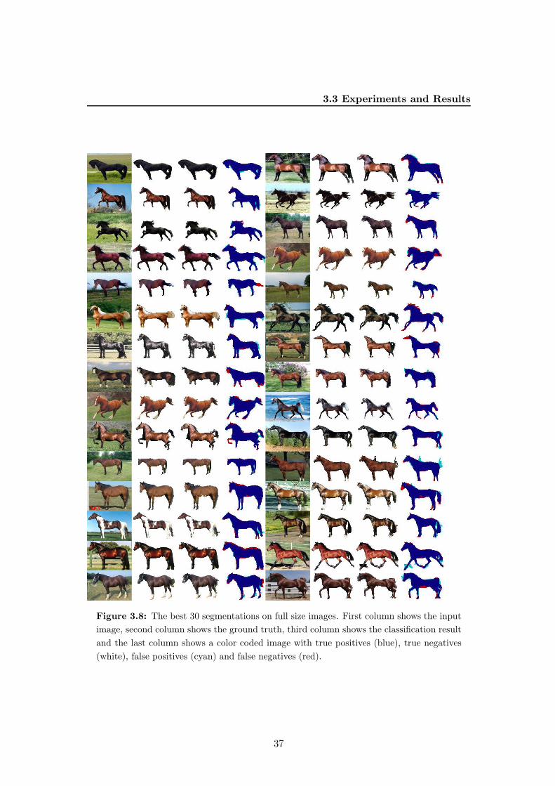
3.3 Experiments and Results
Figure 3.8: The best 30 segmentations on full size images. First column shows the input
image, second column shows the ground truth, third column shows the classification result
and the last column shows a color coded image with true positives (blue), true negatives
(white), false positives (cyan) and false negatives (red).
37
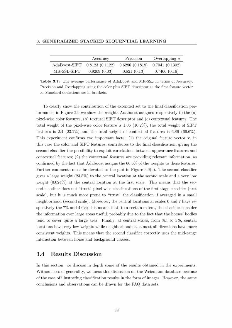
3. GENERALIZED STACKED SEQUENTIAL LEARNING
Accuracy Precision Overlapping o
AdaBoost-SIFT 0.8123 (0.1122) 0.6286 (0.1818) 0.7041 (0.1302)
MR-SSL-SIFT 0.9209 (0.03) 0.821 (0.13) 0.7466 (0.16)
Table 3.7: The average performance of AdaBoost and MR-SSL in terms of Accuracy,
Precision and Overlapping using the color plus SIFT descriptor as the first feature vector
x. Standard deviations are in brackets.
To clearly show the contribution of the extended set to the final classification per-
formance, in Figure 3.9 we show the weights Adaboost assigned respectively to the (a)
pixel-wise color features, (b) textural SIFT descriptor and (c) contextual features. The
total weight of the pixel-wise color feature is 1.06 (10.2%), the total weight of SIFT
features is 2.4 (23.2%) and the total weight of contextual features is 6.89 (66.6%).
This experiment confirms two important facts: (1) the original feature vector x, in
this case the color and SIFT features, contributes to the final classification, giving the
second classifier the possibility to exploit correlations between appearance features and
contextual features; (2) the contextual features are providing relevant information, as
confirmed by the fact that Adaboost assigns the 66.6% of the weights to these features.
Further comments must be devoted to the plot in Figure 3.9(c). The second classifier
gives a large weight (23.5%) to the central location at the second scale and a very low
weight (0.024%) at the central location at the first scale. This means that the sec-
ond classifier does not “trust” pixel-wise classifications of the first stage classifier (first
scale), but it is much more prone to “trust” the classification if averaged in a small
neighborhood (second scale). Moreover, the central locations at scales 6 and 7 have re-
spectively the 7% and 4.6%; this means that, to a certain extent, the classifier consider
the information over large areas useful, probably due to the fact that the horses’ bodies
tend to cover quite a large area. Finally, at central scales, from 3th to 5th, central
locations have very low weights while neighborhoods at almost all directions have more
consistent weights. This means that the second classifier correctly uses the mid-range
interaction between horse and background classes.
3.4 Results Discussion
In this section, we discuss in depth some of the results obtained in the experiments.
Without loss of generality, we focus this discussion on the Weizmann database because
of the ease of illustrating classification results in the form of images. However, the same
conclusions and observations can be drawn for the FAQ data sets.
38
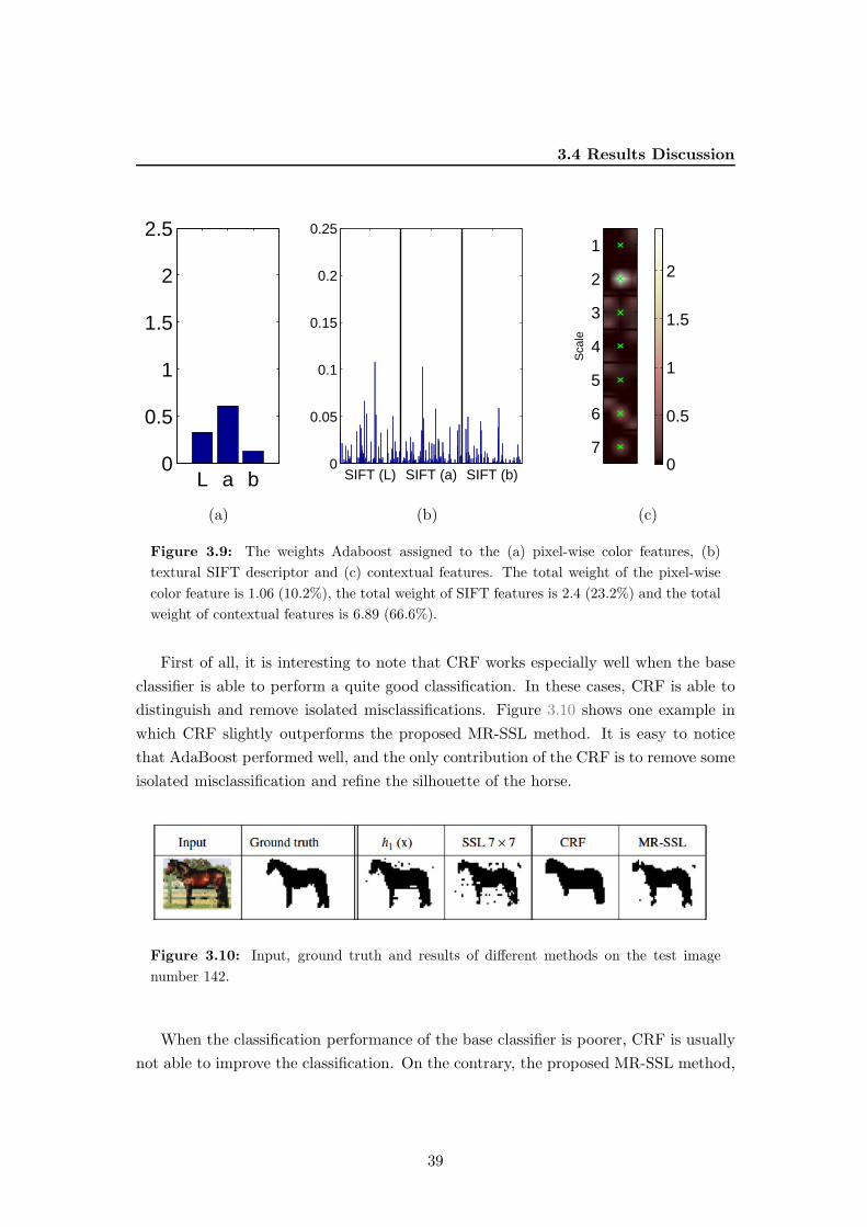
3.4 Results Discussion
L a b0
0.5
1
1.5
2
2.5
SIFT (L) SIFT (a) SIFT (b)0
0.05
0.1
0.15
0.2
0.25
Sca
le
1
2
3
4
5
6
70
0.5
1
1.5
2
(a) (b) (c)
Figure 3.9: The weights Adaboost assigned to the (a) pixel-wise color features, (b)
textural SIFT descriptor and (c) contextual features. The total weight of the pixel-wise
color feature is 1.06 (10.2%), the total weight of SIFT features is 2.4 (23.2%) and the total
weight of contextual features is 6.89 (66.6%).
First of all, it is interesting to note that CRF works especially well when the base
classifier is able to perform a quite good classification. In these cases, CRF is able to
distinguish and remove isolated misclassifications. Figure 3.10 shows one example in
which CRF slightly outperforms the proposed MR-SSL method. It is easy to notice
that AdaBoost performed well, and the only contribution of the CRF is to remove some
isolated misclassification and refine the silhouette of the horse.
Figure 3.10: Input, ground truth and results of different methods on the test image
number 142.
When the classification performance of the base classifier is poorer, CRF is usually
not able to improve the classification. On the contrary, the proposed MR-SSL method,
39
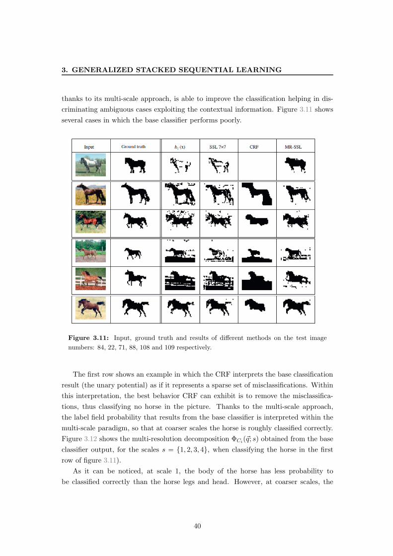
3. GENERALIZED STACKED SEQUENTIAL LEARNING
thanks to its multi-scale approach, is able to improve the classification helping in dis-
criminating ambiguous cases exploiting the contextual information. Figure 3.11 shows
several cases in which the base classifier performs poorly.
Figure 3.11: Input, ground truth and results of different methods on the test image
numbers: 84, 22, 71, 88, 108 and 109 respectively.
The first row shows an example in which the CRF interprets the base classification
result (the unary potential) as if it represents a sparse set of misclassifications. Within
this interpretation, the best behavior CRF can exhibit is to remove the misclassifica-
tions, thus classifying no horse in the picture. Thanks to the multi-scale approach,
the label field probability that results from the base classifier is interpreted within the
multi-scale paradigm, so that at coarser scales the horse is roughly classified correctly.
Figure 3.12 shows the multi-resolution decomposition ΦCi(~q; s) obtained from the base
classifier output, for the scales s = {1, 2, 3, 4}, when classifying the horse in the first
row of figure 3.11).
As it can be noticed, at scale 1, the body of the horse has less probability to
be classified correctly than the horse legs and head. However, at coarser scales, the
40
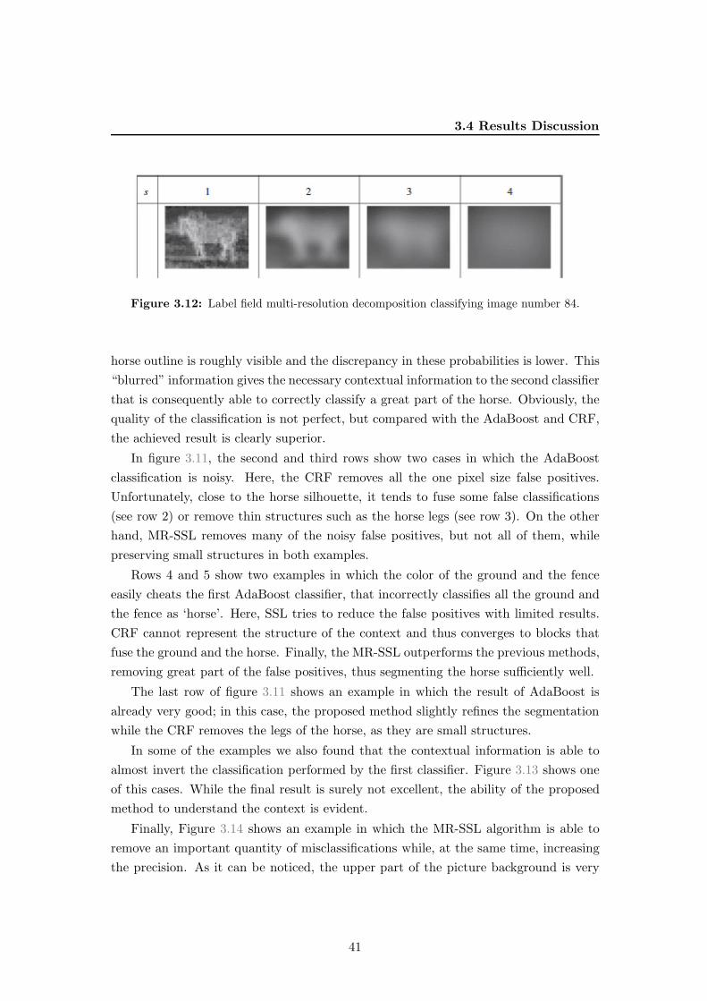
3.4 Results Discussion
Figure 3.12: Label field multi-resolution decomposition classifying image number 84.
horse outline is roughly visible and the discrepancy in these probabilities is lower. This
“blurred” information gives the necessary contextual information to the second classifier
that is consequently able to correctly classify a great part of the horse. Obviously, the
quality of the classification is not perfect, but compared with the AdaBoost and CRF,
the achieved result is clearly superior.
In figure 3.11, the second and third rows show two cases in which the AdaBoost
classification is noisy. Here, the CRF removes all the one pixel size false positives.
Unfortunately, close to the horse silhouette, it tends to fuse some false classifications
(see row 2) or remove thin structures such as the horse legs (see row 3). On the other
hand, MR-SSL removes many of the noisy false positives, but not all of them, while
preserving small structures in both examples.
Rows 4 and 5 show two examples in which the color of the ground and the fence
easily cheats the first AdaBoost classifier, that incorrectly classifies all the ground and
the fence as ‘horse’. Here, SSL tries to reduce the false positives with limited results.
CRF cannot represent the structure of the context and thus converges to blocks that
fuse the ground and the horse. Finally, the MR-SSL outperforms the previous methods,
removing great part of the false positives, thus segmenting the horse sufficiently well.
The last row of figure 3.11 shows an example in which the result of AdaBoost is
already very good; in this case, the proposed method slightly refines the segmentation
while the CRF removes the legs of the horse, as they are small structures.
In some of the examples we also found that the contextual information is able to
almost invert the classification performed by the first classifier. Figure 3.13 shows one
of this cases. While the final result is surely not excellent, the ability of the proposed
method to understand the context is evident.
Finally, Figure 3.14 shows an example in which the MR-SSL algorithm is able to
remove an important quantity of misclassifications while, at the same time, increasing
the precision. As it can be noticed, the upper part of the picture background is very
41
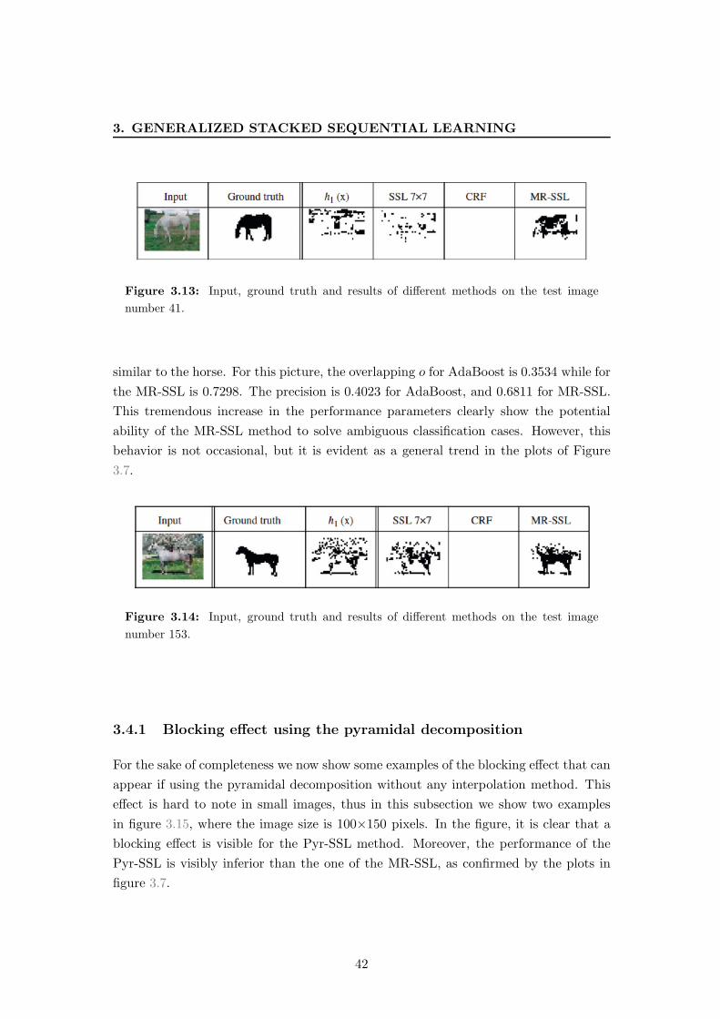
3. GENERALIZED STACKED SEQUENTIAL LEARNING
Figure 3.13: Input, ground truth and results of different methods on the test image
number 41.
similar to the horse. For this picture, the overlapping o for AdaBoost is 0.3534 while for
the MR-SSL is 0.7298. The precision is 0.4023 for AdaBoost, and 0.6811 for MR-SSL.
This tremendous increase in the performance parameters clearly show the potential
ability of the MR-SSL method to solve ambiguous classification cases. However, this
behavior is not occasional, but it is evident as a general trend in the plots of Figure
3.7.
Figure 3.14: Input, ground truth and results of different methods on the test image
number 153.
3.4.1 Blocking effect using the pyramidal decomposition
For the sake of completeness we now show some examples of the blocking effect that can
appear if using the pyramidal decomposition without any interpolation method. This
effect is hard to note in small images, thus in this subsection we show two examples
in figure 3.15, where the image size is 100×150 pixels. In the figure, it is clear that a
blocking effect is visible for the Pyr-SSL method. Moreover, the performance of the
Pyr-SSL is visibly inferior than the one of the MR-SSL, as confirmed by the plots in
figure 3.7.
42
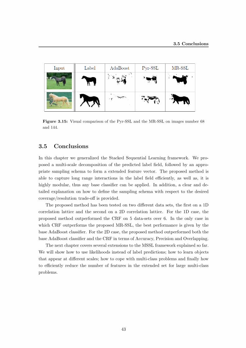
3.5 Conclusions
Figure 3.15: Visual comparison of the Pyr-SSL and the MR-SSL on images number 68
and 144.
3.5 Conclusions
In this chapter we generalized the Stacked Sequential Learning framework. We pro-
posed a multi-scale decomposition of the predicted label field, followed by an appro-
priate sampling schema to form a extended feature vector. The proposed method is
able to capture long range interactions in the label field efficiently, as well as, it is
highly modular, thus any base classifier can be applied. In addition, a clear and de-
tailed explanation on how to define the sampling schema with respect to the desired
coverage/resolution trade-off is provided.
The proposed method has been tested on two different data sets, the first on a 1D
correlation lattice and the second on a 2D correlation lattice. For the 1D case, the
proposed method outperformed the CRF on 5 data-sets over 6. In the only case in
which CRF outperforms the proposed MR-SSL, the best performance is given by the
base AdaBoost classifier. For the 2D case, the proposed method outperformed both the
base AdaBoost classifier and the CRF in terms of Accuracy, Precision and Overlapping.
The next chapter covers several extensions to the MSSL framework explained so far.
We will show how to use likelihoods instead of label predictions; how to learn objects
that appear at different scales; how to cope with multi-class problems and finally how
to efficiently reduce the number of features in the extended set for large multi-class
problems.
43

3. GENERALIZED STACKED SEQUENTIAL LEARNING
44
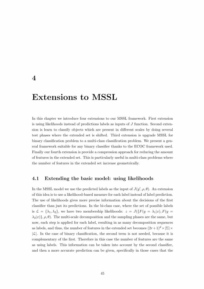
4
Extensions to MSSL
In this chapter we introduce four extensions to our MSSL framework. First extension
is using likelihoods instead of predictions labels as inputs of J function. Second exten-
sion is learn to classify objects which are present in different scales by doing several
test phases where the extended set is shifted. Third extension is upgrade MSSL for
binary classification problem to a multi-class classification problem. We present a gen-
eral framework suitable for any binary classifier thanks to the ECOC framework used.
Finally our fourth extension is provide a compression approach for reducing the amount
of features in the extended set. This is particularly useful in multi-class problems where
the number of features in the extended set increase geometrically.
4.1 Extending the basic model: using likelihoods
In the MSSL model we use the predicted labels as the input of J(y′, ρ, θ). An extension
of this idea is to use a likelihood-based measure for each label instead of label prediction.
The use of likelihoods gives more precise information about the decisions of the first
classifier than just its predictions. In the bi-class case, where the set of possible labels
is L = {λ1, λ2}, we have two membership likelihoods: z = J({F (y = λ1|x), F (y =
λ2|x)}, ρ, θ). The multi-scale decomposition and the sampling phases are the same, but
now, each step is applied for each label, resulting in as many decomposition sequences
as labels, and thus, the number of features in the extended set becomes (2r+1)d×|Σ|×|L|. In the case of binary classification, the second term is not needed, because it is
complementary of the first. Therefore in this case the number of features are the same
as using labels. This information can be taken into account by the second classifier,
and then a more accurate prediction can be given, specifically in those cases that the
45

4. EXTENSIONS TO MSSL
first classifier has limited support for deciding the predicted label.
In order to obtain these values we need the base classifier H1(x) to generate not
only a class prediction, but also its likelihood. Unfortunately, not all kind of classifiers
can give a likelihood for their predictions. However, classifiers that work with margins,
such as Adaboost or SVM, can be used (32). In these cases, it is necessary to con-
vert the margins used by these classifiers to a measure of likelihood. In case of using
Adaboost, we apply a sigmoid function that normalizes Adaboost margins from the
interval [−∞,∞] to [−1, 1] by means of the following equation,
f(x) =1− e−βmx
1 + e−βmx, (4.1)
wheremx is the margin given by Adaboost algorithm for the example x, and a constant
that governs the transition: β = − ln(0.5ǫ)0.25t . It depends on the number of iterations t that
Adaboost performs, and an arbitrary small constant ǫ. Now, we use a soft distance
to convert the normalized values to a likelihood in the range [0, 1] for each label λ as
follows:
f(x|y = λ1) = e−αd(−1,f(x)),
f(x|y = λ2) = e−αd(1,f(x)),
where α = − ln(ǫ)/2 , and ǫ is an arbitrarily small constant (i.e ǫ = 10−3).
4.2 Learning objects at multiple scales
In MSSL the choice of the scales is critical. The more scales are selected, the better
performance is obtained. This is because different patterns at different scales can be
detected. Nonetheless, if we learn a pattern with a concrete size, then when a new
sequence at different size (smaller for example) is classified, the prediction would not
be correct using such scales. This is because the ranges of interactions displayed in
the test sequence are not comparable with the ones displayed in the training phase,
due to the fact that MSSL learns absolute interaction ranges. In order to effectively
learn interactions in the pattern of interest we must ensure that the training set display
these interactions at the same range. We call this particular training set a template.
However, during the testing phase, objects can be found at different sizes displaying
different interaction ranges that the ones learned.
For example, let suppose we have a set of template images X of size D and we
train the model using a set of scales Σ0 = {2, 4, 8}. During the testing phase, let it be
a set of test images X of size D/2 and the same set of scales Σ0 = {2, 4, 8}, then we
46
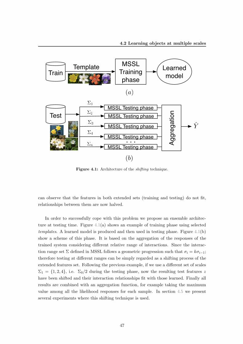
4.2 Learning objects at multiple scales
Learned
modelTrain
Test
Σ1
Σ2
Σ3
Σ4
Σn
MSSL
Training
phase
MSSL Testing phase
MSSL Testing phase
MSSL Testing phase
MSSL Testing phase
MSSL Testing phase
Ag
gre
ga
tio
n
Template
Y
. . .
(a)
(b)
Figure 4.1: Architecture of the shifting technique.
can observe that the features in both extended sets (training and testing) do not fit,
relationships between them are now halved.
In order to successfully cope with this problem we propose an ensemble architec-
ture at testing time. Figure 4.1(a) shows an example of training phase using selected
templates. A learned model is produced and then used in testing phase. Figure 4.1(b)
show a scheme of this phase. It is based on the aggregation of the responses of the
trained system considering different relative range of interactions. Since the interac-
tion range set Σ defined in MSSL follows a geometric progression such that σi = kσi−1;
therefore testing at different ranges can be simply regarded as a shifting process of the
extended features set. Following the previous example, if we use a different set of scales
Σ1 = {1, 2, 4}, i.e. Σ0/2 during the testing phase, now the resulting test features z
have been shifted and their interaction relationships fit with those learned. Finally all
results are combined with an aggregation function, for example taking the maximum
value among all the likelihood responses for each sample. In section 4.5 we present
several experiments where this shifting technique is used.
47

4. EXTENSIONS TO MSSL
4.3 MMSSL: Multi-class Multi-scale Stacked Sequential
Learning
In order to extend the Generalized Stacked Sequential Learning scheme to the multi-
class case,it is necessary that base classifiers H1(x) and H2(x) can deal with data
belonging to N classes instead of just two (binary case). This can be achieved using
inherent multi-class base classifiers such as Random Forests, Naive Bayes, Decision
Trees, Nearest Neighbors, Linear Discriminant Analysis etc. However in those cases
where the base classifiers are not inherently multi class, such as Super Vector Machines
or Regularized Lesat-Squares, a multi-class scheme is needed. The two basics schemes
are: One vs. All and All vs. All. The former consists in building N different binary
classifiers, where for the ith classifier, all the points in class i are the positive examples,
and all the points not in class i are the negative examples. Therefore, let fx be the ith
classifier, the result of classification is to pick the class of the most confident classifier
(Equation 4.2). While the later consists in buildingN(N−1) classifiers, one classifier todistinguish each pair of classes i and j. Let fij be the classifier where class i were positive
examples and class j were negative. Note that exists symmetry between classifiers of
the same pair of classes, i.e. fji = −fij. Therefore the result of classification can be
expressed as in Equation 4.3.
f(x) = argmaxi
fi(x). (4.2)
One vs. All
f(x) = argmaxi
∑
j
fij(x)
. (4.3)
One vs. One
An other approach is using the ECOC framework. Error-Correcting Output Codes
(ECOC) are a general framework to combine binary problems to address the mutli-class
problem (24, 27). ECOC framework consists of two phases: a coding phase, where a
codeword is assigned to each class of a multi-class problem, and a decoding phase,
where, given a test sample, it looks for the most similar class codeword. Originaly (24),
a codeword was a sequence of bits represented by {−1,+1}, where each bit identifies
the membership of the class for a given binary classifier (dichotomizer). Afterwards (3),
a third symbol (the zero symbol) was introduced, which means that a particular class is
not considered by a given classifier. Given a set of N classes to be learned in an ECOC
48
4.3 MMSSL: Multi-class Multi-scale Stacked Sequential Learning
design, n different bipartitions (groups of classes) are formed, and n dichotomizers
over the partitions are trained. As a result, a codeword Yc, c ∈ [1, . . . , N ] of length
n is obtained for each class c. Arranging the codewords as rows, a coding matrix
M ∈ {−1, 0,+1}N×n is defined. The most used coding strategy is the one-versus-all
(50), where each class is discriminated against the rest, obtaining a codeword of length
equal to the number of classes. In Figure 4.2 we show an example of one-versus-one
coding matrix, which considers all possible pairs of classes, with a codeword length
of N(N−1)2 . The matrix is coded using ten dichotomizers {b1, . . . , b10} for a 5-class
problem. The white regions are coded by 1 (considered as one class by the respective
dichotomizer bj , the dark regions by -1 (considered as the other class), and the gray
regions correspond to the zero symbol (classes that are not considered by the respective
dichotomizer bj).
b1 b2 b3 b4 b5 b6 b7 b8 b9 b10
Y1
Y2
Y3
Y4
Y5
Figure 4.2: ECOC one-versus-one coding matrix.
During the decoding process, applying the n binary classifiers, a code X is obtained
for each data sample in the test set. This code is compared to the base codewords
(Yc, c ∈ [1, . . . , N ]) of each class defined in the matrix M . The data sample is then
assigned to the class with the closest codeword. In order to find the closest codeword,
the decoding strategies most frequently used are Hamming and Euclidean measures
(28). those based on distances measurements between the output code and the target
codeword. Among these, the most applied(27) are defined as: HD(x, yi) =∑n
j=1(1 −sign(xj · yji ))/2; defined as: ED(x, yi) =
√∑n
j=1(xj − yji )
2.
Apart from the extension of the base classifiers, the neighborhood function J(y′, ρ, θ)
has also to be modified. Figure 4.3 shows the Multi-class Multi-scale Stacked Sequential
Learning (MMSSL) scheme presented in this work. Given an input sample x, the
first classifier produces not only a prediction, but a measure of confidence F (x, c)
for belonging to each class defined in c ∈ [1, . . . , N ]. These confidence maps are the
input of the neighborhood function J(F (x, c), ρ,Σ). This function performs a multi-
class decomposition over the confidence maps into s scales defined by Σ. Over this
49
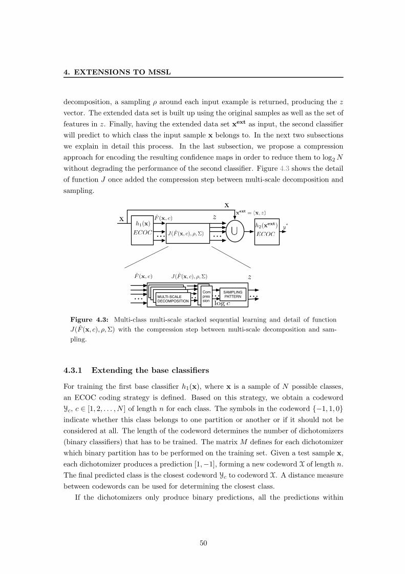
4. EXTENSIONS TO MSSL
decomposition, a sampling ρ around each input example is returned, producing the z
vector. The extended data set is built up using the original samples as well as the set of
features in z. Finally, having the extended data set xext as input, the second classifier
will predict to which class the input sample x belongs to. In the next two subsections
we explain in detail this process. In the last subsection, we propose a compression
approach for encoding the resulting confidence maps in order to reduce them to log2N
without degrading the performance of the second classifier. Figure 4.3 shows the detail
of function J once added the compression step between multi-scale decomposition and
sampling.
ECOC ECOCJ(F (x, c), ρ,Σ). . .
zF (x, c)
. . .
SAMPLING PATTERN. . .
F (x, c) z
. . .
log c
. . . . . .MULTI-SCALE DECOMPOSITION
Compression
J(F (x, c), ρ,Σ)
h1(x) h2(xext)
Figure 4.3: Multi-class multi-scale stacked sequential learning and detail of function
J(F (x, c), ρ,Σ) with the compression step between multi-scale decomposition and sam-
pling.
4.3.1 Extending the base classifiers
For training the first base classifier h1(x), where x is a sample of N possible classes,
an ECOC coding strategy is defined. Based on this strategy, we obtain a codeword
Yc, c ∈ [1, 2, . . . , N ] of length n for each class. The symbols in the codeword {−1, 1, 0}indicate whether this class belongs to one partition or another or if it should not be
considered at all. The length of the codeword determines the number of dichotomizers
(binary classifiers) that has to be trained. The matrix M defines for each dichotomizer
which binary partition has to be performed on the training set. Given a test sample x,
each dichotomizer produces a prediction [1,−1], forming a new codeword X of length n.
The final predicted class is the closest codeword Yc to codeword X. A distance measure
between codewords can be used for determining the closest class.
If the dichotomizers only produce binary predictions, all the predictions within
50

4.3 MMSSL: Multi-class Multi-scale Stacked Sequential Learning
X have the same importance. Instead, if the dichotomizers can produce a measure
of confidence on its predictions, a more fine-grained distance between codewords can
be obtained. By applying equation 4.1 we can convert the margins used by those
classifiers to a measure of confidence with values between the codeword interval [−1, 1].Applying this for each dichotomizer, a new codeword X of length n is formed, where
all the symbols ∈ R. Once we have a normalized codeword, we use a soft distance δ
for decoding, i.e. we compare the codeword X with each codeword Yc, c ∈ [1, . . . , N ]
defined in the matrixM . These distance measures can be seen as a prediction confidence
measure for each class, once we normalize them to the range [0, 1]. Therefore, given a
set of possible labels ci, i ∈ [1, . . . , N ], we define the membership confidences as follows:
F (y = ci|x) = e−αδ(Y1,X),∀i ∈ [1, .., N ], (4.4)
where δ is a soft distance such the Euclidean one, and α depends on δ. By applying this
to the all data samples in X we define the confidence map for each class as expressed
in Equation 4.5:
F (x, c) = {F (y = c1|x), . . . , F (y = cN |x)},∀x ∈ X. (4.5)
4.3.2 Extending the neighborhood function J
We define the neighborhood function J in two stages: 1) a multi-scale decomposition
over the confidence maps F (x, c) and 2) a sampling performed over the multi-scale
representation. This function is extended in order to deal with multiple classes. Now
it is formulated as follows:
z = J(F (x, c), ρ,Σ).
Starting from the confidence maps, we apply a multi-scale decomposition upon them,
resulting in as many decomposition sequences as classes. For the decomposition we
use the multi-resolution Gaussian approach (3.2.1.1). Each level of the decomposition
(scale) is generated by the convolution of the confidence map by a Gaussian mask with
standard deviation σ. In this way, the bigger σ is, the longer interactions are considered.
Therefore, at each level of decomposition all the points have information from the rest
accordingly to the sigma parameter. Given a set of Σ = {σ1, . . . , σs} ∈ R+ and all
the predicted confidence maps F (x, c), each level of the decomposition si, i ∈ [1, . . . , s]
is computed as follows:
F si(x, c) = gσi(x) ∗ F (x, c),∀i ∈ [1, .., s],
51

4. EXTENSIONS TO MSSL
where gσi(x) is defined as a multidimensional isotropic gaussian filter with zero
mean:
gσi(x) =1
(2π)d/2σ1/2i
e−12xT σ−1
ix.
Once the multi-scale decomposition is performed, we define the support lattice z.
This is, the sampling over the multi-scale representation which forms the extended
data. Our choice is to use a scale-space sliding window over each label multi-scale
decomposition. The selected window has a fixed radius with length defined by ρ in each
dimension d and with origin in the current prediction example. Thus, the elements
covered by the window is w = (2ρ + 1)d around the origin. Then, for each scale si
considered in the previous decomposition the window is stretched in each direction
using a displacement proportional to the scale we are analyzing. This displacement
at each scale forces that each point considered around the current prediction has very
small influence from previous neighbor points. In this way, the number of features of
z appended to the input data set is equal to (2ρ+ 1)d · s · c. According to this, we can
see that the extended data set increases with the number of classes. This can produce
a scalability problem, since the second classifier has to deal with large feature sets.
4.4 Extended data set grouping: a compression approach
The goal of grouping the extended data set is to compress its number of features without
losing significant performance. Using our MMSSL approach, we can see that the size
of the extended set depends on the number of classes, the number of scales, and the
number of samples around each example. We can choose the number of samples and
scales, but the number of classes is problem dependent. Therefore, for reducing the
number of confidence maps, we add a compression process between the multi-scale
decomposition and the sampling process as shown in Figure 4.3. This compression is
done following information theory by means of partitions.
Let P be a set {{P 11 , P
21 }, . . . , {P 1
κ , P2κ}} of partitions groups of classes and c =
{c1, . . . , cN} the set of all the classes, so that for any j, P 1j ⊆ c, P 2
j ⊆ c | P 1j ∪ P 2
j = c,
and P 1j ∩ P 2
j = ∅. The confidence maps are grouped using the elements on P. We
have defined two different ways of combining the partitions: using binary compression
or using ternary compression. Let the confidence map F sk of a certain scale sk, k ∈[1, . . . , s] be expressed as follows,
F sk(x, Pj) =
N∑
i
γijFsk(x, ci), (4.6)
52
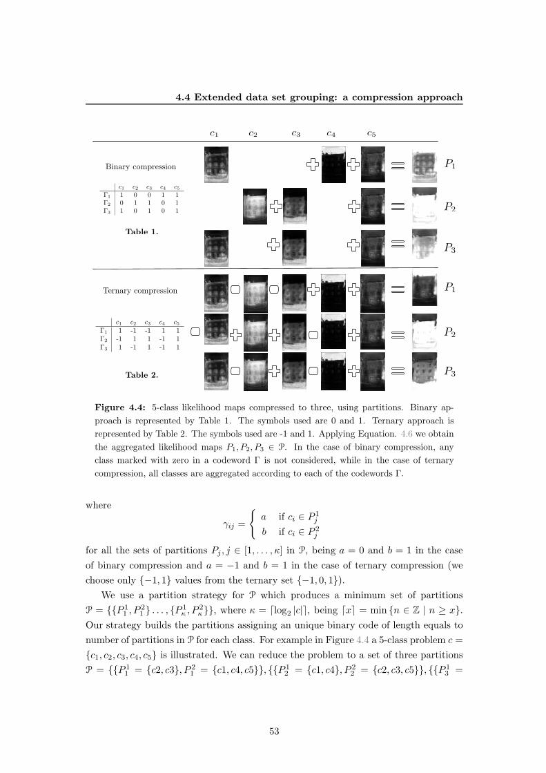
4.4 Extended data set grouping: a compression approach
c1 c2 c3 c4 c5
c1 c2 c3 c4 c5
Γ1 1 0 0 1 1
Γ2 0 1 1 0 1
Γ3 1 0 1 0 1
c1 c2 c3 c4 c5
Γ1 1 -1 -1 1 1
Γ2 -1 1 1 -1 1
Γ3 1 -1 1 -1 1
Table 1.
Table 2.
P1
P1
P2
P3
P3
P2
Binary compression
Ternary compression
Figure 4.4: 5-class likelihood maps compressed to three, using partitions. Binary ap-
proach is represented by Table 1. The symbols used are 0 and 1. Ternary approach is
represented by Table 2. The symbols used are -1 and 1. Applying Equation. 4.6 we obtain
the aggregated likelihood maps P1, P2, P3 ∈ P. In the case of binary compression, any
class marked with zero in a codeword Γ is not considered, while in the case of ternary
compression, all classes are aggregated according to each of the codewords Γ.
where
γij =
{
a if ci ∈ P 1j
b if ci ∈ P 2j
for all the sets of partitions Pj , j ∈ [1, . . . , κ] in P, being a = 0 and b = 1 in the case
of binary compression and a = −1 and b = 1 in the case of ternary compression (we
choose only {−1, 1} values from the ternary set {−1, 0, 1}).We use a partition strategy for P which produces a minimum set of partitions
P = {{P 11 , P
21 } . . . , {P 1
κ , P2κ}}, where κ = ⌈log2 |c|⌉, being ⌈x⌉ = min {n ∈ Z | n ≥ x}.
Our strategy builds the partitions assigning an unique binary code of length equals to
number of partitions in P for each class. For example in Figure 4.4 a 5-class problem c =
{c1, c2, c3, c4, c5} is illustrated. We can reduce the problem to a set of three partitions
P = {{P 11 = {c2, c3}, P 2
1 = {c1, c4, c5}}, {{P 12 = {c1, c4}, P 2
2 = {c2, c3, c5}}, {{P 13 =
53
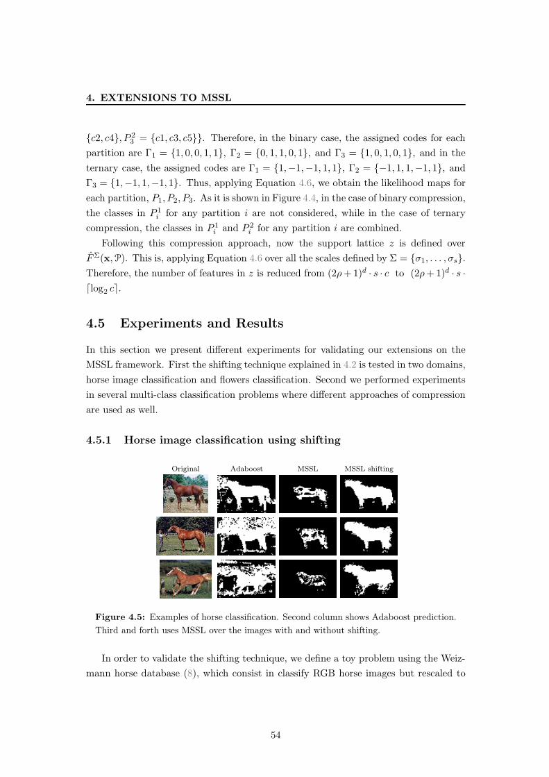
4. EXTENSIONS TO MSSL
{c2, c4}, P 23 = {c1, c3, c5}}. Therefore, in the binary case, the assigned codes for each
partition are Γ1 = {1, 0, 0, 1, 1}, Γ2 = {0, 1, 1, 0, 1}, and Γ3 = {1, 0, 1, 0, 1}, and in the
ternary case, the assigned codes are Γ1 = {1,−1,−1, 1, 1}, Γ2 = {−1, 1, 1,−1, 1}, andΓ3 = {1,−1, 1,−1, 1}. Thus, applying Equation 4.6, we obtain the likelihood maps for
each partition, P1, P2, P3. As it is shown in Figure 4.4, in the case of binary compression,
the classes in P 1i for any partition i are not considered, while in the case of ternary
compression, the classes in P 1i and P 2
i for any partition i are combined.
Following this compression approach, now the support lattice z is defined over
FΣ(x,P). This is, applying Equation 4.6 over all the scales defined by Σ = {σ1, . . . , σs}.Therefore, the number of features in z is reduced from (2ρ+1)d · s · c to (2ρ+1)d · s ·⌈log2 c⌉.
4.5 Experiments and Results
In this section we present different experiments for validating our extensions on the
MSSL framework. First the shifting technique explained in 4.2 is tested in two domains,
horse image classification and flowers classification. Second we performed experiments
in several multi-class classification problems where different approaches of compression
are used as well.
4.5.1 Horse image classification using shifting
Original Adaboost MSSL MSSL shifting
Figure 4.5: Examples of horse classification. Second column shows Adaboost prediction.
Third and forth uses MSSL over the images with and without shifting.
In order to validate the shifting technique, we define a toy problem using the Weiz-
mann horse database (8), which consist in classify RGB horse images but rescaled to
54
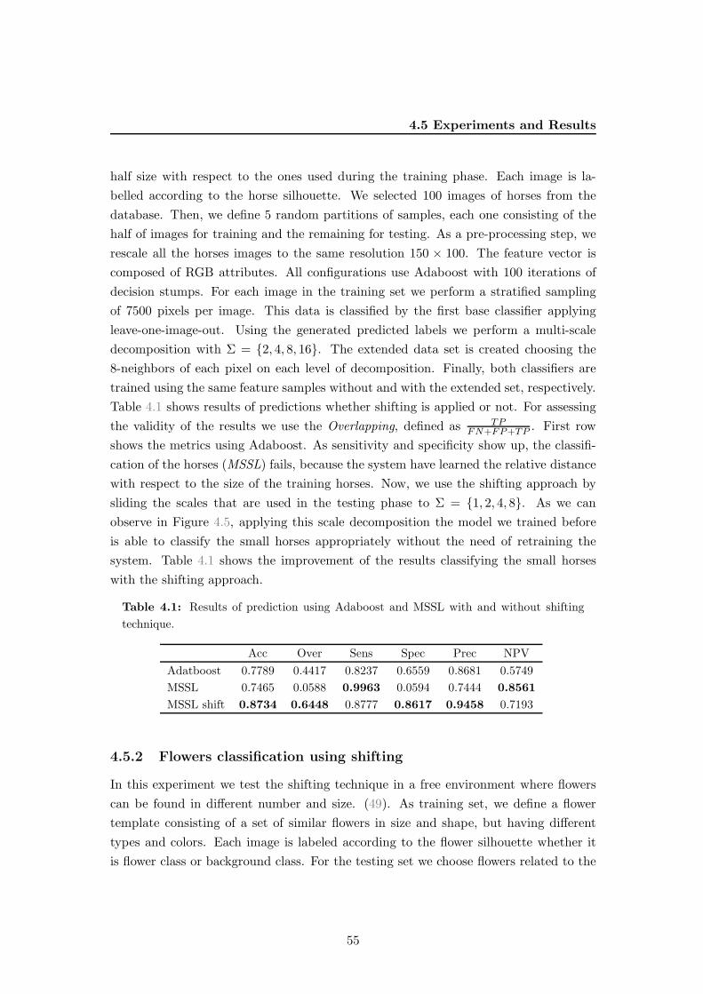
4.5 Experiments and Results
half size with respect to the ones used during the training phase. Each image is la-
belled according to the horse silhouette. We selected 100 images of horses from the
database. Then, we define 5 random partitions of samples, each one consisting of the
half of images for training and the remaining for testing. As a pre-processing step, we
rescale all the horses images to the same resolution 150 × 100. The feature vector is
composed of RGB attributes. All configurations use Adaboost with 100 iterations of
decision stumps. For each image in the training set we perform a stratified sampling
of 7500 pixels per image. This data is classified by the first base classifier applying
leave-one-image-out. Using the generated predicted labels we perform a multi-scale
decomposition with Σ = {2, 4, 8, 16}. The extended data set is created choosing the
8-neighbors of each pixel on each level of decomposition. Finally, both classifiers are
trained using the same feature samples without and with the extended set, respectively.
Table 4.1 shows results of predictions whether shifting is applied or not. For assessing
the validity of the results we use the Overlapping, defined as TPFN+FP+TP . First row
shows the metrics using Adaboost. As sensitivity and specificity show up, the classifi-
cation of the horses (MSSL) fails, because the system have learned the relative distance
with respect to the size of the training horses. Now, we use the shifting approach by
sliding the scales that are used in the testing phase to Σ = {1, 2, 4, 8}. As we can
observe in Figure 4.5, applying this scale decomposition the model we trained before
is able to classify the small horses appropriately without the need of retraining the
system. Table 4.1 shows the improvement of the results classifying the small horses
with the shifting approach.
Table 4.1: Results of prediction using Adaboost and MSSL with and without shifting
technique.
Acc Over Sens Spec Prec NPV
Adatboost 0.7789 0.4417 0.8237 0.6559 0.8681 0.5749
MSSL 0.7465 0.0588 0.9963 0.0594 0.7444 0.8561
MSSL shift 0.8734 0.6448 0.8777 0.8617 0.9458 0.7193
4.5.2 Flowers classification using shifting
In this experiment we test the shifting technique in a free environment where flowers
can be found in different number and size. (49). As training set, we define a flower
template consisting of a set of similar flowers in size and shape, but having different
types and colors. Each image is labeled according to the flower silhouette whether it
is flower class or background class. For the testing set we choose flowers related to the
55
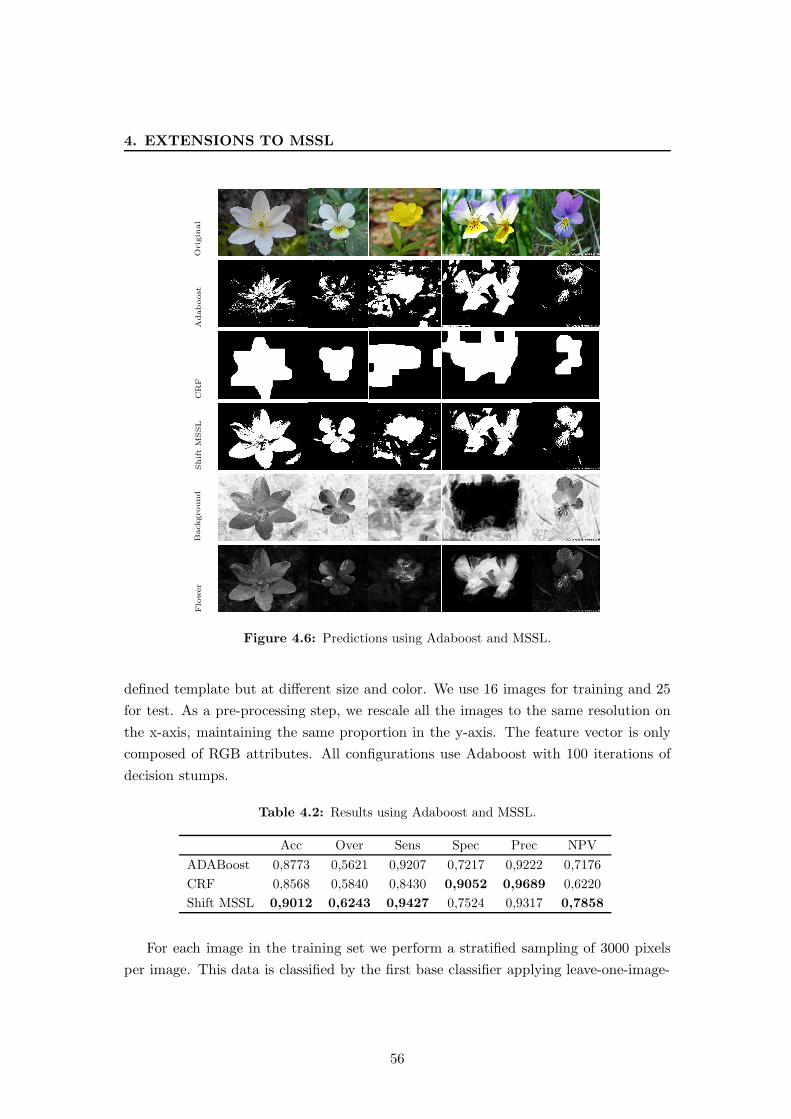
4. EXTENSIONS TO MSSL
Origin
al
Adaboost
CRF
ShiftM
SSL
Background
Flower
Figure 4.6: Predictions using Adaboost and MSSL.
defined template but at different size and color. We use 16 images for training and 25
for test. As a pre-processing step, we rescale all the images to the same resolution on
the x-axis, maintaining the same proportion in the y-axis. The feature vector is only
composed of RGB attributes. All configurations use Adaboost with 100 iterations of
decision stumps.
Table 4.2: Results using Adaboost and MSSL.
Acc Over Sens Spec Prec NPV
ADABoost 0,8773 0,5621 0,9207 0,7217 0,9222 0,7176
CRF 0,8568 0,5840 0,8430 0,9052 0,9689 0,6220
Shift MSSL 0,9012 0,6243 0,9427 0,7524 0,9317 0,7858
For each image in the training set we perform a stratified sampling of 3000 pixels
per image. This data is classified by the first base classifier applying leave-one-image-
56
4.5 Experiments and Results
out. Using the generated predicted labels we perform a multi-scale decomposition with
Σ = {18, 27, 41}. The extended data set is created choosing the 8-neighbors of each
pixel on each level of decomposition. Finally, both classifiers are trained using the same
feature samples with and without the extended set, respectively. We have performed
several testing phases using always the same trained model. For each testing phase,
we use a three scale decomposition from the range Σ = {0.5, 3, 5, 8, 12, 18, 27, 41}. This
makes a total of 6 test rounds per image. At the end of each test round we take the
measures of the likelihood of each image. Examples of background and flower likelihoods
images at different rounds are shown in Figure 4.6. We calculate the maximum for all
rounds, resulting in two images. The row Shift MSSL shows the result of joining both
images using the greater than operation. The figure also shows the original image and
its resulting classification using Adaboost and CRF (45). Table 4.2 shows the metrics
for these methods. Shift MSSL approach beats the non-sequential Adaboost approach
for each metric and it also beats CRF in accuracy and overlapping. The rest of metrics
point out that our method is better defining the flower class than the CRF method.
4.5.3 MSSL for multi-class classification problems
In the next subsection data, methods and validation protocol for each experiment are
presented. Afterwards, the results are presented in two aspects, a) statistical results,
where different measures are computed and significance tests are performed on different
datasets, and b) qualitative results, where concrete results are particularly analyzed for
a more intuitive understanding of the behavior of each method.
4.5.3.1 Experimental Settings
• Data: we test our multi-class methodology performing 9 different experiments
out from four databases:
1. Sensor Motion data database: The sensor motion database (14) is a data set
of accelerometer sensor runs from 15 different people performing certain ac-
tivities. Each accelerometer sample is labeled as one of 5 different activities,
namely walking, climbing stairs, standing idle, interacting and working. The
spatial relationship in label space is 1D. There are two different scenarios.
Sequential scenario is where all the people is doing the activities in the same
order (motion sequential scenario). Random scenario is where all the people
is performing the activities in random order (motion random scenario)). We
57
4. EXTENSIONS TO MSSL
also performed a third experiment for benchmark purposes in which there
are only activities from one person (motion one person).
2. FAQ database (17, 26): The FAQ database is a set of frequented asked
questions pages from Usenet. There are 48 annotated pages from several
topics. Each line in a page is labeled as (0) header, (1) question, (2) answer,
or (3) tailing. There are 24 boolean features characterizing each line. The
spatial relationship in label space is 1D.
3. IVUS image database (16): It contains images from Intravascular Ultra-
sound (IVUS). They are a set of IVUS frames manually labelled. 8 classes
are considered: (1) blood, (2) plaque, (3) media, (4) media adventitia, (5)
guide-wire, (6) shadowing, (7) external tissue, and (8) calcium. The spa-
tial relationship in label space is 2D. There are 29 textural features in total
extracted from IVUS data.
4. e-trims database (41): The e-trims database is comprised of two image
datasets, e-trims 4-class with four annotated object classes and e-trims 8-
class with eight annotated object classes. There are 60 annotated images in
each of the dataset. The object classes considered in 4-class dataset are: (1)
building, (2) pavement/road, (3) sky, and (4) vegetation. In 8-class dataset
the object classes considered are: (1) building, (2) car, (3) door, (4) pave-
ment, (5) road, (6) sky, (7) vegetation, and (8) window. Additionally, for
each database we have a background class (0) for any other object. All
images are resized proportionally to 150 pixels height. Train images are
stratified sampled, taking 3000 pixels. We have performed experiments with
two different set of features: RGB representation of each pixel, and RGB
plus HOG (Histogram of oriented gradient (19)) with 9 bins, ending up with
12 features for sample. The spatial relationship in label space is 2D.
• Methods: We test all the databases with four different configurations of our
MMSSL methodology. Also, we test with Real Adaboost (31) and CRF Multi-
label optimization through Graph Cut α-expansion (10) as baseline experiments.
The settings for all the MMSSL configurations are the same, the only difference
is the way the extended data set is generated. We have used as base classi-
fier a Real Adaboost ensemble of 100 decision stumps. The coding strategy
for the ECOC framework in each classifier is one-versus-one and the decoding
measure is Euclidean distance. The neighborhood function performs a Gaussian
multi-resolution decomposition in 4 scales, using Σ = {1, 2, 4, 8}, except in IVUS
58
4.5 Experiments and Results
database where we used 6 scales Σ = {1, 2, 4, 8, 16, 32} due to the images di-
mensions. In 1D databases, we used w = 7 elements in both directions of the
neighborhood, while in 2D databases we used just the surrounding points, i.e.
w = 1. Summarizing, the different experiments we have performed are:
1. MMSSL using labels. It uses the MMSSL framework using only the predicted
labels from the first classifier as input for neighborhood function.
2. MMSSL using confidences. It uses the MMSSL framework using the confi-
dence maps for all the classes as input for neighborhood function.
3. MMSSL using compression approach with binary matrix: It uses the MMSSL
framework using a compression over the confidence map. The compression
matrix uses binary values {0, 1}.4. MMSSL using compression approach with ternary matrix. It uses the MMSSL
framework using a compression over the confidence map. The compression
matrix uses ternary values {−1, 1}.5. Adaboost. Uses only one Adaboost classifier, without taking into account
the neighborhood relationship. Used as baseline experiment.
6. Multi-label optimization. It uses multi-label optimization via α-expansion.
We have applied the α-expansion optimization, using the confidence maps
for each class obtained from the first classifier. For the neighborhood term,
we use the intensity between the point and its neighbors for each direction
defined in the database.
• Validation: For the different experiments we use 5-fold cross-validation or one-
leave-out for final prediction. For each fold, the base classifier h1(x) uses ten-fold
cross-validation for predicting the labels of the training set, which produces the
confidence maps used later for the second classifier h2(x). We measure the results
in terms of the accuracy, and the mean of overlapping, recall, and precision from
a N × N confusion matrix , computed as follow: accuracy =∑N
i TPi∑N
i (TP+FP+FN)i,
overlappingi =TPi
(TP+FN+FP )i, recalli =
TPi
(TP+FN)i, and precisioni =
TPi
(FP+TP )i,
where TPi means the predictions correctly classified in the class i, FPi means the
predictions misclassified as class i and FNi means the actual class i predictions
misclassified as any other class. For comparing the results obtained from the
different experiments we have used statistic tests: the Friedman test for checking
the non-randomness of the results and the Nemenyi test for checking if one of the
configurations can be statistically singled out (23).
59
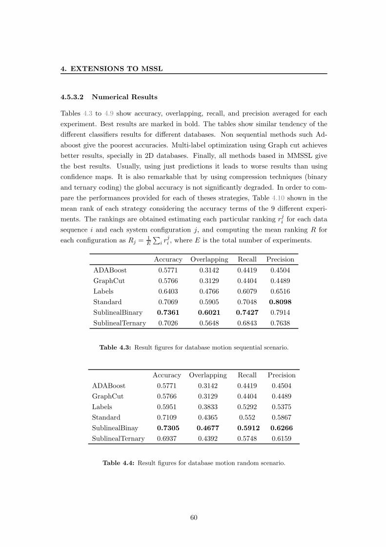
4. EXTENSIONS TO MSSL
4.5.3.2 Numerical Results
Tables 4.3 to 4.9 show accuracy, overlapping, recall, and precision averaged for each
experiment. Best results are marked in bold. The tables show similar tendency of the
different classifiers results for different databases. Non sequential methods such Ad-
aboost give the poorest accuracies. Multi-label optimization using Graph cut achieves
better results, specially in 2D databases. Finally, all methods based in MMSSL give
the best results. Usually, using just predictions it leads to worse results than using
confidence maps. It is also remarkable that by using compression techniques (binary
and ternary coding) the global accuracy is not significantly degraded. In order to com-
pare the performances provided for each of theses strategies, Table 4.10 shown in the
mean rank of each strategy considering the accuracy terms of the 9 different experi-
ments. The rankings are obtained estimating each particular ranking rji for each data
sequence i and each system configuration j, and computing the mean ranking R for
each configuration as Rj =1E
∑
i rji , where E is the total number of experiments.
Accuracy Overlapping Recall Precision
ADABoost 0.5771 0.3142 0.4419 0.4504
GraphCut 0.5766 0.3129 0.4404 0.4489
Labels 0.6403 0.4766 0.6079 0.6516
Standard 0.7069 0.5905 0.7048 0.8098
SublinealBinary 0.7361 0.6021 0.7427 0.7914
SublinealTernary 0.7026 0.5648 0.6843 0.7638
Table 4.3: Result figures for database motion sequential scenario.
Accuracy Overlapping Recall Precision
ADABoost 0.5771 0.3142 0.4419 0.4504
GraphCut 0.5766 0.3129 0.4404 0.4489
Labels 0.5951 0.3833 0.5292 0.5375
Standard 0.7109 0.4365 0.552 0.5867
SublinealBinay 0.7305 0.4677 0.5912 0.6266
SublinealTernary 0.6937 0.4392 0.5748 0.6159
Table 4.4: Result figures for database motion random scenario.
60
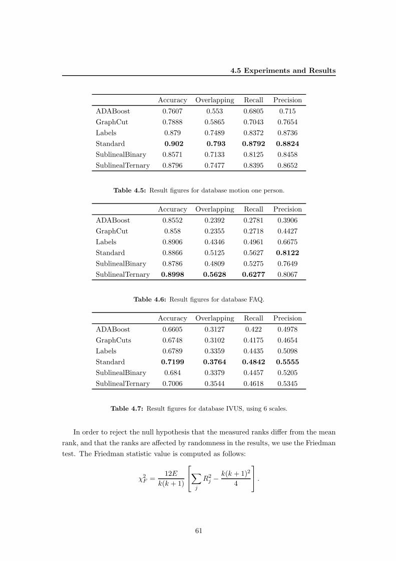
4.5 Experiments and Results
Accuracy Overlapping Recall Precision
ADABoost 0.7607 0.553 0.6805 0.715
GraphCut 0.7888 0.5865 0.7043 0.7654
Labels 0.879 0.7489 0.8372 0.8736
Standard 0.902 0.793 0.8792 0.8824
SublinealBinary 0.8571 0.7133 0.8125 0.8458
SublinealTernary 0.8796 0.7477 0.8395 0.8652
Table 4.5: Result figures for database motion one person.
Accuracy Overlapping Recall Precision
ADABoost 0.8552 0.2392 0.2781 0.3906
GraphCut 0.858 0.2355 0.2718 0.4427
Labels 0.8906 0.4346 0.4961 0.6675
Standard 0.8866 0.5125 0.5627 0.8122
SublinealBinary 0.8786 0.4809 0.5275 0.7649
SublinealTernary 0.8998 0.5628 0.6277 0.8067
Table 4.6: Result figures for database FAQ.
Accuracy Overlapping Recall Precision
ADABoost 0.6605 0.3127 0.422 0.4978
GraphCuts 0.6748 0.3102 0.4175 0.4654
Labels 0.6789 0.3359 0.4435 0.5098
Standard 0.7199 0.3764 0.4842 0.5555
SublinealBinary 0.684 0.3379 0.4457 0.5205
SublinealTernary 0.7006 0.3544 0.4618 0.5345
Table 4.7: Result figures for database IVUS, using 6 scales.
In order to reject the null hypothesis that the measured ranks differ from the mean
rank, and that the ranks are affected by randomness in the results, we use the Friedman
test. The Friedman statistic value is computed as follows:
χ2F =
12E
k(k + 1)
∑
j
R2j −
k(k + 1)2
4
.
61
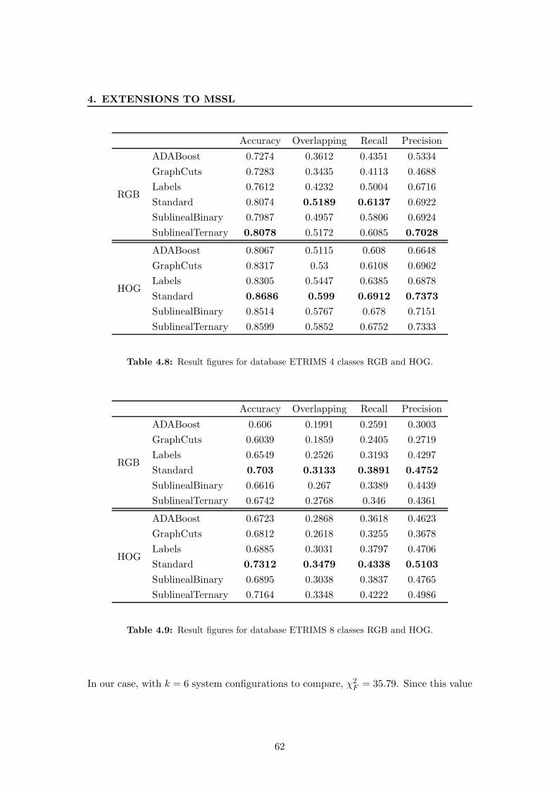
4. EXTENSIONS TO MSSL
Accuracy Overlapping Recall Precision
RGB
ADABoost 0.7274 0.3612 0.4351 0.5334
GraphCuts 0.7283 0.3435 0.4113 0.4688
Labels 0.7612 0.4232 0.5004 0.6716
Standard 0.8074 0.5189 0.6137 0.6922
SublinealBinary 0.7987 0.4957 0.5806 0.6924
SublinealTernary 0.8078 0.5172 0.6085 0.7028
HOG
ADABoost 0.8067 0.5115 0.608 0.6648
GraphCuts 0.8317 0.53 0.6108 0.6962
Labels 0.8305 0.5447 0.6385 0.6878
Standard 0.8686 0.599 0.6912 0.7373
SublinealBinary 0.8514 0.5767 0.678 0.7151
SublinealTernary 0.8599 0.5852 0.6752 0.7333
Table 4.8: Result figures for database ETRIMS 4 classes RGB and HOG.
Accuracy Overlapping Recall Precision
RGB
ADABoost 0.606 0.1991 0.2591 0.3003
GraphCuts 0.6039 0.1859 0.2405 0.2719
Labels 0.6549 0.2526 0.3193 0.4297
Standard 0.703 0.3133 0.3891 0.4752
SublinealBinary 0.6616 0.267 0.3389 0.4439
SublinealTernary 0.6742 0.2768 0.346 0.4361
HOG
ADABoost 0.6723 0.2868 0.3618 0.4623
GraphCuts 0.6812 0.2618 0.3255 0.3678
Labels 0.6885 0.3031 0.3797 0.4706
Standard 0.7312 0.3479 0.4338 0.5103
SublinealBinary 0.6895 0.3038 0.3837 0.4765
SublinealTernary 0.7164 0.3348 0.4222 0.4986
Table 4.9: Result figures for database ETRIMS 8 classes RGB and HOG.
In our case, with k = 6 system configurations to compare, χ2F = 35.79. Since this value
62
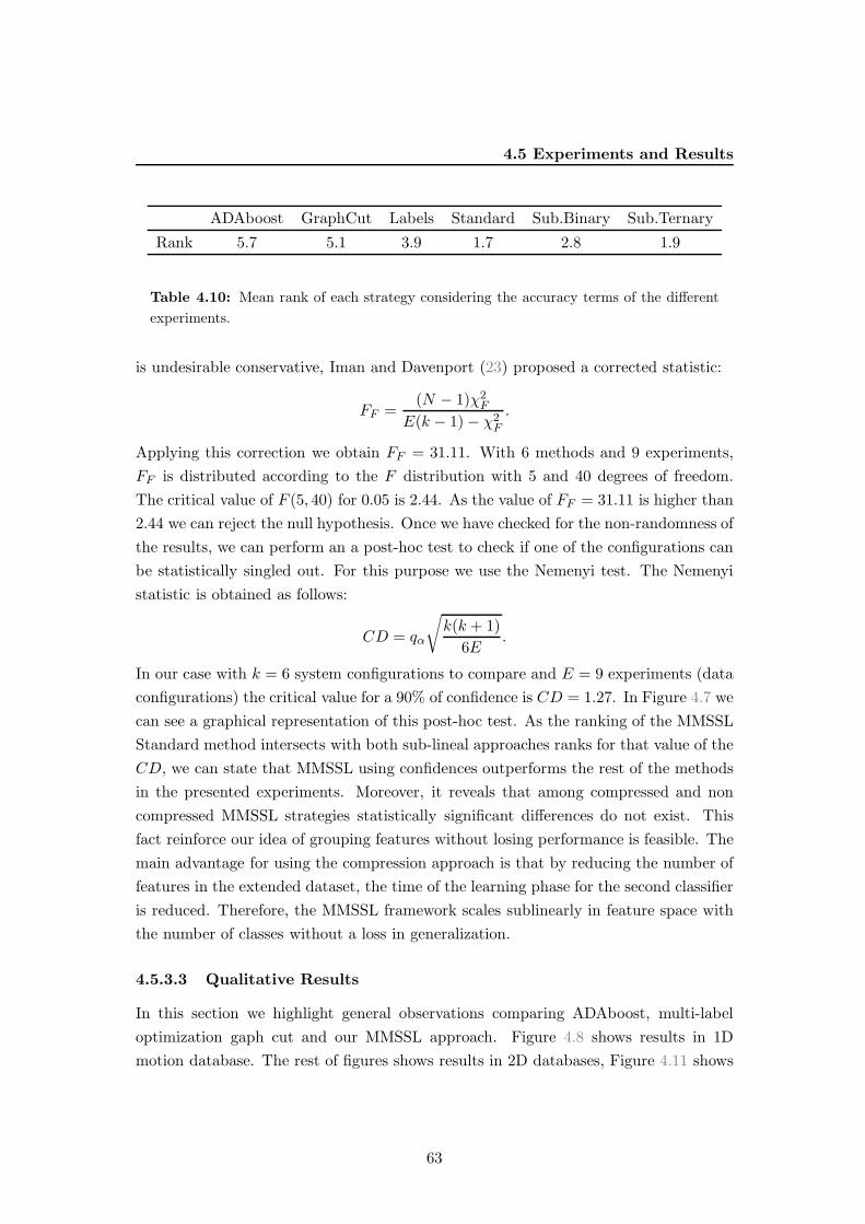
4.5 Experiments and Results
ADAboost GraphCut Labels Standard Sub.Binary Sub.Ternary
Rank 5.7 5.1 3.9 1.7 2.8 1.9
Table 4.10: Mean rank of each strategy considering the accuracy terms of the different
experiments.
is undesirable conservative, Iman and Davenport (23) proposed a corrected statistic:
FF =(N − 1)χ2
F
E(k − 1)− χ2F
.
Applying this correction we obtain FF = 31.11. With 6 methods and 9 experiments,
FF is distributed according to the F distribution with 5 and 40 degrees of freedom.
The critical value of F (5, 40) for 0.05 is 2.44. As the value of FF = 31.11 is higher than
2.44 we can reject the null hypothesis. Once we have checked for the non-randomness of
the results, we can perform an a post-hoc test to check if one of the configurations can
be statistically singled out. For this purpose we use the Nemenyi test. The Nemenyi
statistic is obtained as follows:
CD = qα
√
k(k + 1)
6E.
In our case with k = 6 system configurations to compare and E = 9 experiments (data
configurations) the critical value for a 90% of confidence is CD = 1.27. In Figure 4.7 we
can see a graphical representation of this post-hoc test. As the ranking of the MMSSL
Standard method intersects with both sub-lineal approaches ranks for that value of the
CD, we can state that MMSSL using confidences outperforms the rest of the methods
in the presented experiments. Moreover, it reveals that among compressed and non
compressed MMSSL strategies statistically significant differences do not exist. This
fact reinforce our idea of grouping features without losing performance is feasible. The
main advantage for using the compression approach is that by reducing the number of
features in the extended dataset, the time of the learning phase for the second classifier
is reduced. Therefore, the MMSSL framework scales sublinearly in feature space with
the number of classes without a loss in generalization.
4.5.3.3 Qualitative Results
In this section we highlight general observations comparing ADAboost, multi-label
optimization gaph cut and our MMSSL approach. Figure 4.8 shows results in 1D
motion database. The rest of figures shows results in 2D databases, Figure 4.11 shows
63
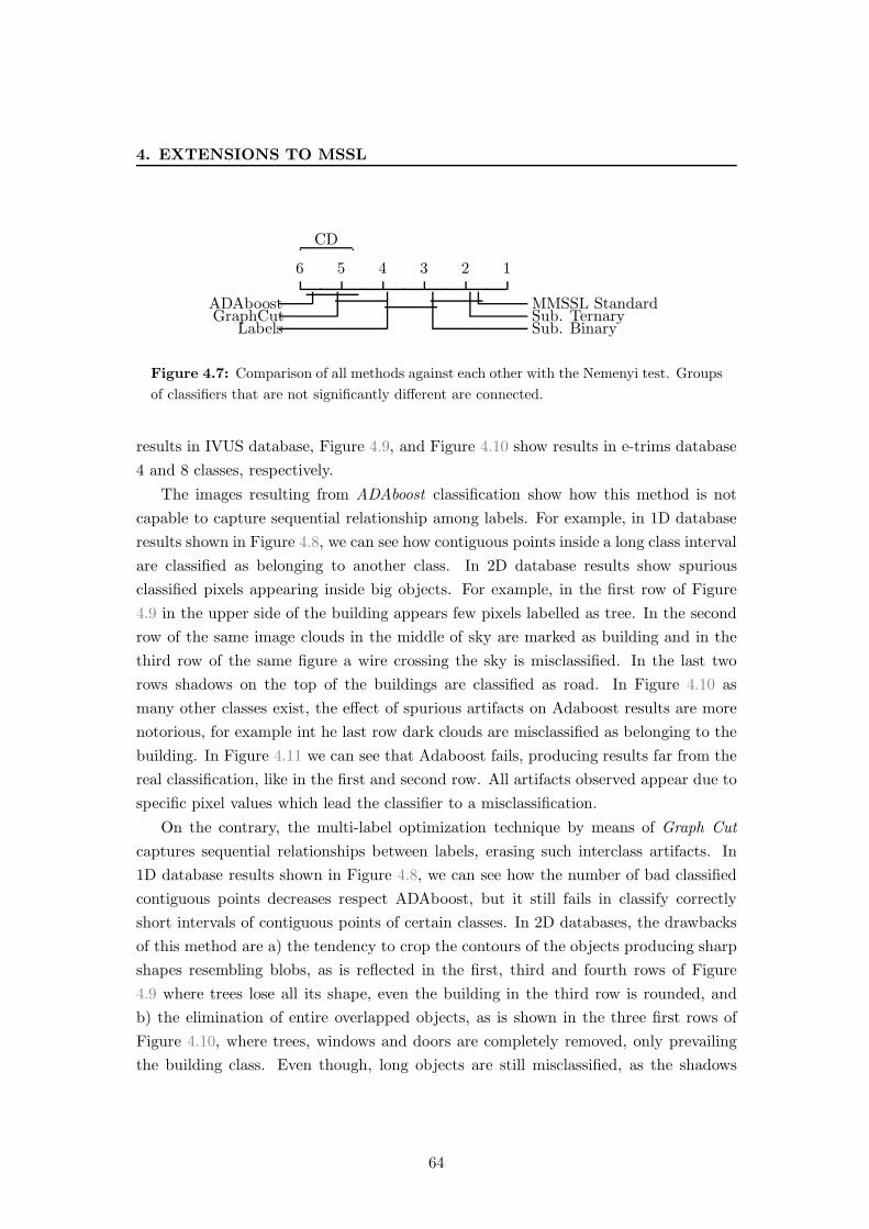
4. EXTENSIONS TO MSSL
6 5 4 3 2 1
CD
ADAboostGraphCut
Labels Sub. BinarySub. TernaryMMSSL Standard
Figure 4.7: Comparison of all methods against each other with the Nemenyi test. Groups
of classifiers that are not significantly different are connected.
results in IVUS database, Figure 4.9, and Figure 4.10 show results in e-trims database
4 and 8 classes, respectively.
The images resulting from ADAboost classification show how this method is not
capable to capture sequential relationship among labels. For example, in 1D database
results shown in Figure 4.8, we can see how contiguous points inside a long class interval
are classified as belonging to another class. In 2D database results show spurious
classified pixels appearing inside big objects. For example, in the first row of Figure
4.9 in the upper side of the building appears few pixels labelled as tree. In the second
row of the same image clouds in the middle of sky are marked as building and in the
third row of the same figure a wire crossing the sky is misclassified. In the last two
rows shadows on the top of the buildings are classified as road. In Figure 4.10 as
many other classes exist, the effect of spurious artifacts on Adaboost results are more
notorious, for example int he last row dark clouds are misclassified as belonging to the
building. In Figure 4.11 we can see that Adaboost fails, producing results far from the
real classification, like in the first and second row. All artifacts observed appear due to
specific pixel values which lead the classifier to a misclassification.
On the contrary, the multi-label optimization technique by means of Graph Cut
captures sequential relationships between labels, erasing such interclass artifacts. In
1D database results shown in Figure 4.8, we can see how the number of bad classified
contiguous points decreases respect ADAboost, but it still fails in classify correctly
short intervals of contiguous points of certain classes. In 2D databases, the drawbacks
of this method are a) the tendency to crop the contours of the objects producing sharp
shapes resembling blobs, as is reflected in the first, third and fourth rows of Figure
4.9 where trees lose all its shape, even the building in the third row is rounded, and
b) the elimination of entire overlapped objects, as is shown in the three first rows of
Figure 4.10, where trees, windows and doors are completely removed, only prevailing
the building class. Even though, long objects are still misclassified, as the shadows
64

4.5 Experiments and Results
in the top part of the buildings in the last two rows in Figure 4.9, or worst, the dark
clouds in the last row of Figure 4.10 are completely joined with the building forming a
huge building. In Figure 4.11 we can see a fairly improvement respect Adaboost, but it
still fails in the classification of the three first rows. This method fails mainly because
it is not considering the relationship among objects at different scales.
The last method considered is our approach, MMSSL using confidences without
compression.The results of this method are qualitatively better than the rest. The
results are a trade-off between spacial coherence and shape permanence. This is because
the relationship among classes is considered at different scales. In 1D database results
shown in Figure 4.8, we can see how the MMSSL is the only method that achieves good
performance as well in long sequences as in short sequences of points of the same class
and does not matter whether the activities are carried on in the same order as trained or
not. In 2D databases, we can see in Figure 4.9 how MMSSL is able to keep the shape
of buildings and trees in all the images and how it removes interclass artifacts that
previous method were not able to, for example the shadows on the top of the building
in the last two rows. In Figure 4.10 we can see in all the images that windows, trees
and doors are fairly kept, even the dark clouds in the last row are practically removed,
appearing only spurious pixels in the border of the image. Moreover, in Figure 4.11, we
can see how MMSSL is able to close big areas of the same class like in the three firsts
rows, where the rest of methods fail. Also is remarkable in the fourth and fifth row
how narrower classes between wider classes are preserved, where the other methods fail.
The points where the method fails the most are the junctions between classes where
does not exist a clear distinction, for example in the second row in Figure 4.10 where
cars are classified altogether as one, mixing with the grass and the road.
65
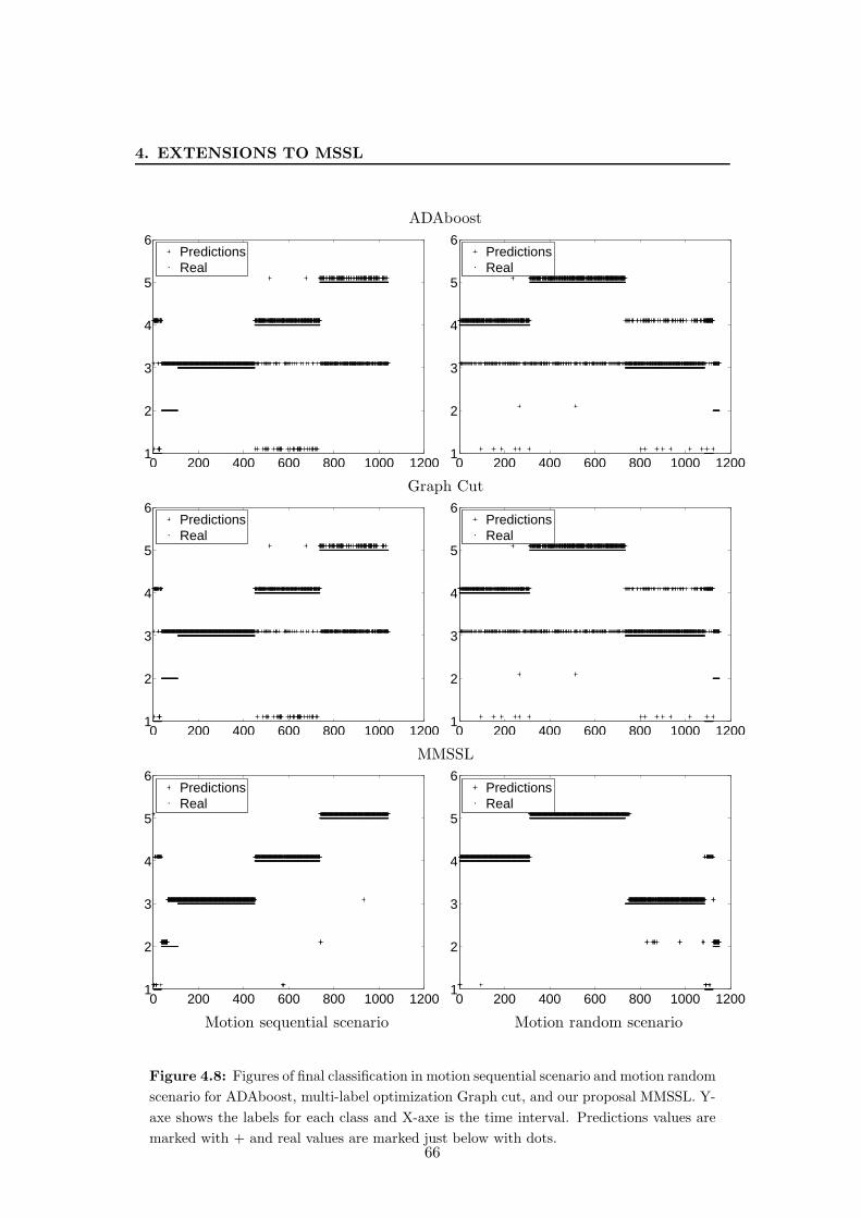
4. EXTENSIONS TO MSSL
ADAboost
0 200 400 600 800 1000 12001
2
3
4
5
6
PredictionsReal
0 200 400 600 800 1000 12001
2
3
4
5
6
PredictionsReal
Graph Cut
0 200 400 600 800 1000 12001
2
3
4
5
6
PredictionsReal
0 200 400 600 800 1000 12001
2
3
4
5
6
PredictionsReal
MMSSL
0 200 400 600 800 1000 12001
2
3
4
5
6
PredictionsReal
0 200 400 600 800 1000 12001
2
3
4
5
6
PredictionsReal
Motion sequential scenario Motion random scenario
Figure 4.8: Figures of final classification in motion sequential scenario and motion random
scenario for ADAboost, multi-label optimization Graph cut, and our proposal MMSSL. Y-
axe shows the labels for each class and X-axe is the time interval. Predictions values are
marked with + and real values are marked just below with dots.66
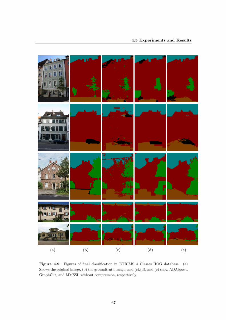
4.5 Experiments and Results
(a) (b) (c) (d) (e)
Figure 4.9: Figures of final classification in ETRIMS 4 Classes HOG database. (a)
Shows the original image, (b) the groundtruth image, and (c),(d), and (e) show ADAboost,
GraphCut, and MMSSL without compression, respectively.
67
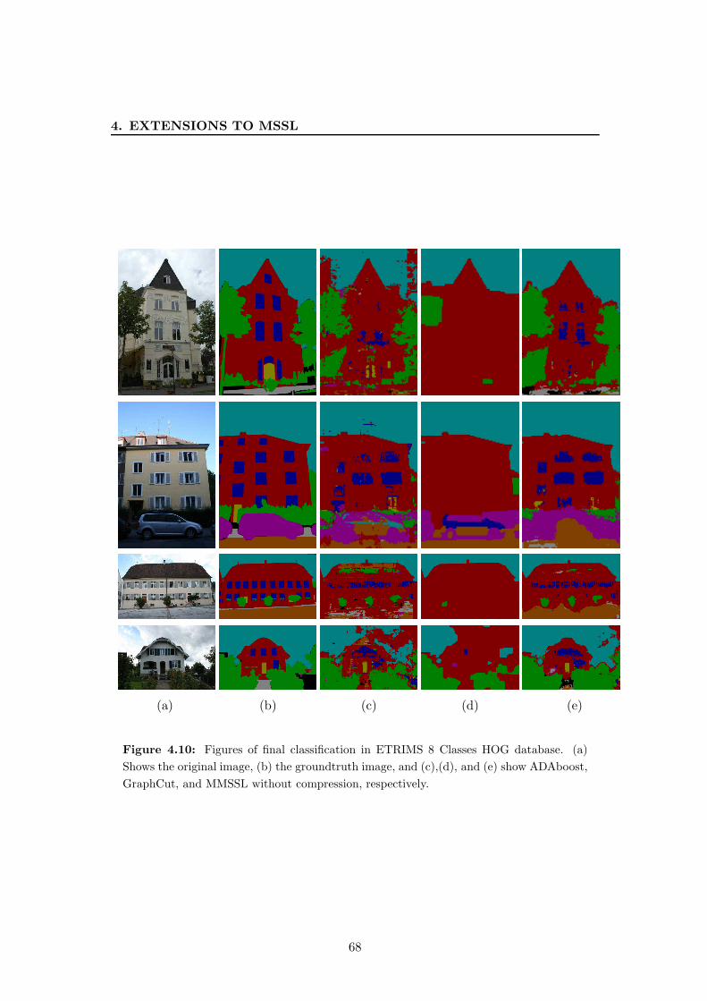
4. EXTENSIONS TO MSSL
(a) (b) (c) (d) (e)
Figure 4.10: Figures of final classification in ETRIMS 8 Classes HOG database. (a)
Shows the original image, (b) the groundtruth image, and (c),(d), and (e) show ADAboost,
GraphCut, and MMSSL without compression, respectively.
68
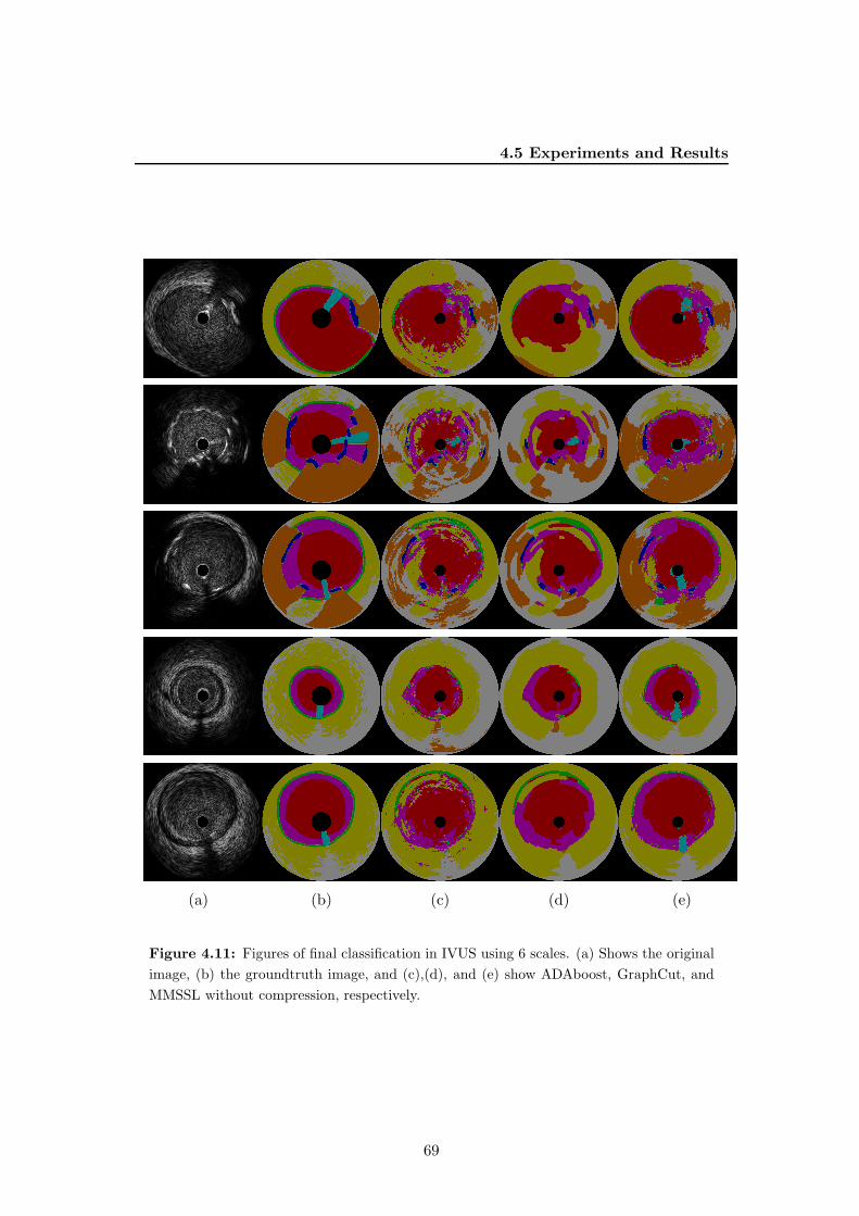
4.5 Experiments and Results
(a) (b) (c) (d) (e)
Figure 4.11: Figures of final classification in IVUS using 6 scales. (a) Shows the original
image, (b) the groundtruth image, and (c),(d), and (e) show ADAboost, GraphCut, and
MMSSL without compression, respectively.
69
4. EXTENSIONS TO MSSL
4.5.3.4 Comparing among proposed multi-class MSSL techniques
Finally, Figures 4.12 and 4.13 show the difference among MMSSL approaches. It is
appreciable how MMSSL using labels fails classifying long areas of contiguous pixels,
while the rest of methods predict them correctly. This is because using confidences
for each sample instead of the most probable label makes possible to break ties of
equiprobable classes. Differences between compressed and non compressed methods
are not so straightforward to see, but while in Figure 4.12 there are few differences
in Figure 4.13 we can see how non compressed methods leads to smoother results
than compressed methods. Compressed methods tend to fail in closing some classes,
appearing spurious pixels inside them. Sometimes this behavior can lead to a better
classification if it was misclassified, as it happens in the last row of Figure 4.12. The
second row of Figure 4.13 shows the learning capacity of the likelihood maps. In column
(d), MMSSL without compression, we can see a boundary marked as unknown object
(class 0, black label) in front of the building. Inside this region, it is marked as car label.
In the original image, column (a), it is appreciable a woman riding a bicycle in those
area. Although in the groundtruth image, column (b), these elements are omitted, our
method using likelihood maps is capable of detecting them as an element different to
road or building, and assigning the inner region to car label, given its visual appearance
and position.
70
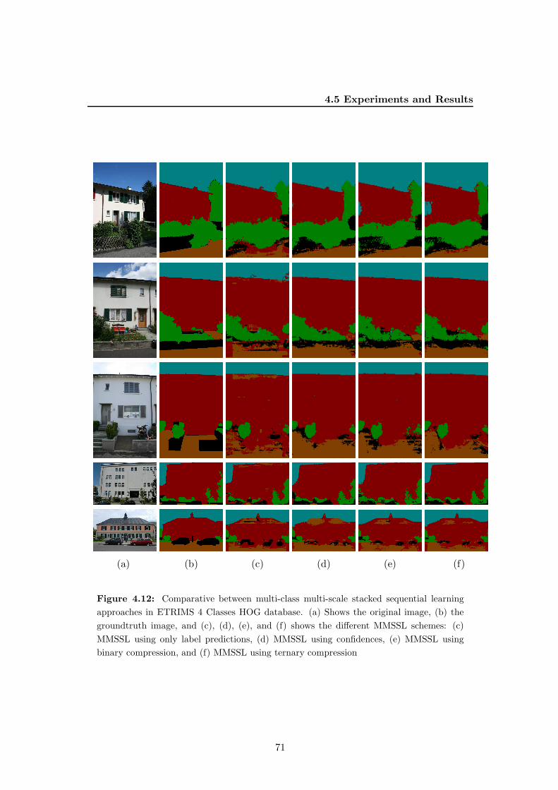
4.5 Experiments and Results
(a) (b) (c) (d) (e) (f)
Figure 4.12: Comparative between multi-class multi-scale stacked sequential learning
approaches in ETRIMS 4 Classes HOG database. (a) Shows the original image, (b) the
groundtruth image, and (c), (d), (e), and (f) shows the different MMSSL schemes: (c)
MMSSL using only label predictions, (d) MMSSL using confidences, (e) MMSSL using
binary compression, and (f) MMSSL using ternary compression
71
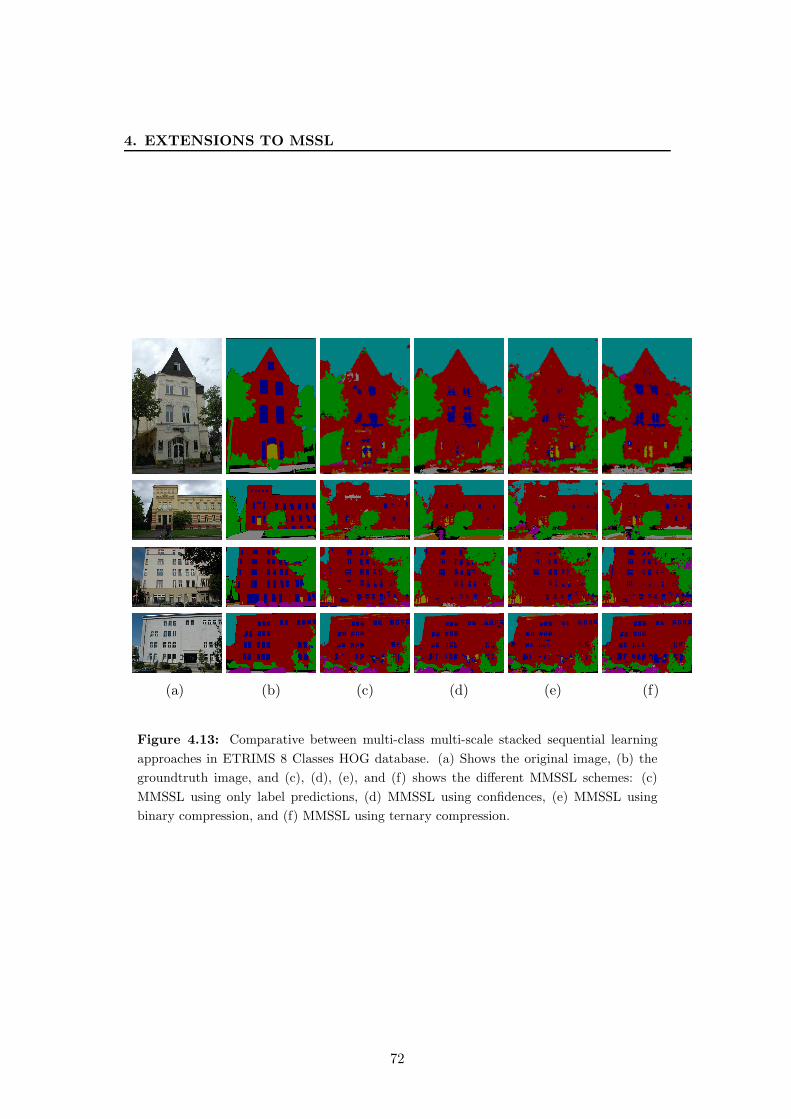
4. EXTENSIONS TO MSSL
(a) (b) (c) (d) (e) (f)
Figure 4.13: Comparative between multi-class multi-scale stacked sequential learning
approaches in ETRIMS 8 Classes HOG database. (a) Shows the original image, (b) the
groundtruth image, and (c), (d), (e), and (f) shows the different MMSSL schemes: (c)
MMSSL using only label predictions, (d) MMSSL using confidences, (e) MMSSL using
binary compression, and (f) MMSSL using ternary compression.
72
4.6 Conclusions
4.6 Conclusions
In this chapter we extended the Multi-scale stacked sequential learning framework in
different ways. First we adapt the J for working with likelihood values instead of
prediction labels when the first classifier is able to produce them. Secondly we adjust
the MSSL framework for classifying objects at different sizes. In order to do this, we
proposed the shifting technique at testing time. This allows to correctly classify objects
at different sizes than the learned ones. Thirdly, we adapt the multi-scale sequential
learning (MSSL) to the multi-class case (MMSSL). In order to do this, we put the
ECOC framework into the base classifiers and show how to compute the confidence
maps using the normalized margins obtained from the ECOC base classifiers. Finally we
define a compression approach for reducing the number of features in the extended data
set. The results show that, on the one hand, MMSSL achieves accurate classification
performance in multi-class classification problems taking benefit of sequential learning.
On the other hand, the compression process is feasible, since in terms of accuracy the
loss of information is negligible.
In next chapter we present an example application of MSSL for human body segmen-
tation, where exists sequential dependences between instances. In this scenario MSSL is
used with great success, improving results with respect state-of-the-art methodologies.
73

4. EXTENSIONS TO MSSL
74
5
Application of MSSL for human
body segmentation
Human segmentation in RGB images is a challenging task due to the high variability
of the human body, which includes a wide range of human poses, lighting conditions,
cluttering, clothes, appearance, background, point of view, number of human body
limbs, etc. In this particular problem, the goal is to provide a complete segmentation
of the person/people appearing in an image. In literature, human body segmentation
is usually treated in a two-stage fashion. First, a human body part detection step is
performed, obtaining a large set of candidate body parts. These parts are used as prior
knowledge by segmentation/inference optimization algorithms in order to obtain the
final human body segmentation.
In the first stage, that is the detection of body parts, weak classifiers are trained
in order to obtain a soft prior of body parts (which are often noisy and unreliable).
Most works in literature have used edge detectors, convolutions with filters, linear SVM
classifiers, Adaboost or Cascading classifiers (67). For example, (58) used a tubular
edge template as a detector, and convolved it with an image defining locally maximal
responses above a threshold as detections. In (57), the authors used quadratic logistic
regression on RGB features as the part detectors. Other works, have applied more
robust part detectors such as SVM classifiers (15, 35) or AdaBoost (51) trained on
HOG features (19). More recently, Dantone et. al used Random Forest as classifiers
to learn body parts (20). Although recently robust classifiers have been used, part
detectors still involve false-positive and false-negatives problems given the similarity
nature among body parts and the presence of background artifacts. Therefore, a second
stage is usually required in order to provide an accurate segmentation.
75
5. APPLICATION OF MSSL FOR HUMAN BODY SEGMENTATION
In the second stage, soft part detections are jointly optimized taking into account
the nature of the human body. However, standard segmentation techniques (i.e. region-
growing, thresholding, edge detection, etc.) are not applicable in this context due to
the huge variability of environmental factors (i.e lightning, clothing, cluttering, etc.)
and the changing nature of body textures. In this sense, the most known models for
the optimization/inference of soft part priors are Poselets (9, 51) of Bourdev et. al.
and Pictorial Structures (4, 30, 62) by Felzenszwalb et. al., both of which optimize the
initial soft body part priors to obtain a more accurate estimation of the human pose,
and provide with a multi-limb detection. In addition, there are some works in literature
that tackle the problem of human body segmentation (segmenting the full body as one
class) obtaining satisfying results. For instance, Vinet et al. (66) proposed to use
Conditional Random Fields (CRF) based on body part detectors to obtain a complete
person/background segmentation. Belief propagation, branch and bound or Graph Cut
optimization are common approaches used to perform inference of the graphical models
defined by human body (38, 39, 59). Finally, methods like structured SVM or mixture
of parts (72, 73) can be use in order to take profit of the contextual relations of body
parts.
In this chapter, we present a novel two-stage human body segmentation method
based on the Multi-Scale Stacked Sequential Learning (MSSL) framework. In the first
stage of our method for human segmentation, a multi-class Error-Correcting Output
Codes classifier (ECOC) is trained to detect body parts and to produce a soft likelihood
map for each body part. In the second stage, a multi-scale decomposition of these
maps and a neighborhood sampling is performed, resulting in a new set of features.
The extended set of features encodes spatial, contextual and relational information
among body parts. This extended set is then fed to the second classifier of MSSL, in
this case a Random Forest binary classifier, which maps a multi-limb classification to
a binary human classification problem. Finally, in order to obtain the resulting binary
human segmentation, a post-processing step is performed by means of Graph Cuts
optimization, which is applied to the output of the binary classifier.
5.1 Stage One: Body Parts Soft Detection
In this work, the first stage detector H1(x) in the MSSL pipeline is based on the soft
body parts detectors defined in (60). The work of Bautista et al (60) is based on
an ECOC ensemble of cascades of Adaboost classifiers. Each of the cascades focuses
on a subset of body parts described using Haar-like features where regions have been
76

5.1 Stage One: Body Parts Soft Detection
previously rotated towards main orientation to make the recognition rotation invariant.
Although any other part detector technique could be used in the first stage of our
process, we also choose the same methodology. As a case study, although any classifier
can be included in the ECOC framework, here we considerer as base learner also the
same ensemble of cascades given its fast computization.
Because of its properties, cascades of classifiers are usually trained to split one visual
object from the rest of possible objects of an image. This means that the cascade of
classifiers learns to detect a certain object (body part in our case), ignoring all other
objects (all other body parts). However, some body parts have similar appearance, i.e.
legs and arms, and thus, it makes sense to group them in the same visual category.
Because of this, we learn a set of cascades of classifiers where a subset of limbs are
included in the positive set of one cascade, and the remaining limbs are included as
negative instances together with background images in the negative set of the cascade.
In this sense, classifier H1 is learned by grouping different cascades of classifiers in a
tree-structure way and combining them in an Error-Correcting Output Codes (ECOC)
framework (28). Then, H1 outputs correspond to a multi-limb classification prediction.
An example of the body part tree-structure defined taking into account the nature
of human body parts is shown in Fig. 5.2(a). Notice that classes with similar visual
appearance (e.g. upper-arm and lower-arm) are grouped in the same meta-class in most
dichotomies. In addition, dichotomies that deal with difficult problems (e.g. d5) are
focused only in the difficult classes, without taking into account all other body parts.
In this case, class c7 denotes the background.
We use the problem dependent coding matrix defined in (60) in order to allow
the inclusion of cascade of classifiers and learn the body parts. In particular, each
dichotomy is obtained from the body part tree-structure. Fig. 5.2(b) shows the coding
matrix codification of the tree-structure in Fig. 5.2(a).
In the ECOC decoding step an image is processed using a sliding windowing ap-
proach. Each image patch x, is described and tested. In our case, each patch is first
rotated by main gradient orientation and tested using the ECOC ensemble with Haar-
like features and cascade of classifier. In this sense, each classifier d outputs a prediction
whether x belongs to one of the two previously learnt meta-classes. Once the set of
predictions c ∈ {+1,−1}1×n is obtained, it is compared to the set of codewords of the
classes yi from M , using a decoding function δ(c, yi) and the final prediction is the
class with the codeword with minimum decoding, i.e. argmini δ(c, yi). As a decoding
function we use the Loss-Weighted approach with linear loss function defined in (28).
Then, a body-like probability map is built. This map contains, at each position the
77
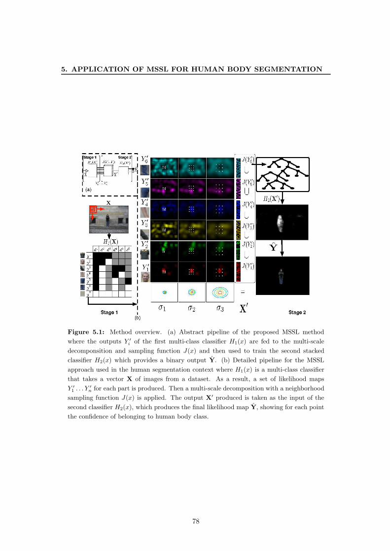
5. APPLICATION OF MSSL FOR HUMAN BODY SEGMENTATION
Figure 5.1: Method overview. (a) Abstract pipeline of the proposed MSSL method
where the outputs Y ′
iof the first multi-class classifier H1(x) are fed to the multi-scale
decomponsition and sampling function J(x) and then used to train the second stacked
classifier H2(x) which provides a binary output Y. (b) Detailed pipeline for the MSSL
approach used in the human segmentation context where H1(x) is a multi-class classifier
that takes a vector X of images from a dataset. As a result, a set of likelihood maps
Y ′
1. . . Y ′
n for each part is produced. Then a multi-scale decomposition with a neighborhood
sampling function J(x) is applied. The output X′ produced is taken as the input of the
second classifier H2(x), which produces the final likelihood map Y, showing for each point
the confidence of belonging to human body class.
78
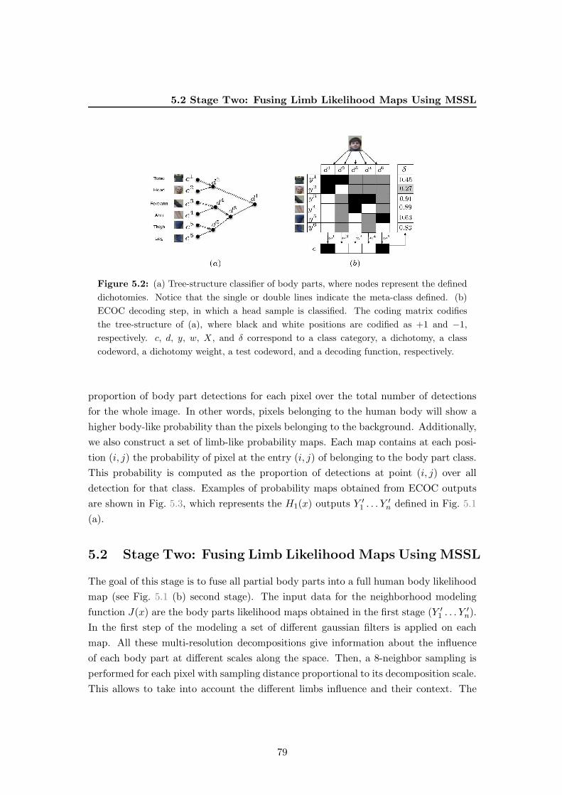
5.2 Stage Two: Fusing Limb Likelihood Maps Using MSSL
Figure 5.2: (a) Tree-structure classifier of body parts, where nodes represent the defined
dichotomies. Notice that the single or double lines indicate the meta-class defined. (b)
ECOC decoding step, in which a head sample is classified. The coding matrix codifies
the tree-structure of (a), where black and white positions are codified as +1 and −1,respectively. c, d, y, w, X , and δ correspond to a class category, a dichotomy, a class
codeword, a dichotomy weight, a test codeword, and a decoding function, respectively.
proportion of body part detections for each pixel over the total number of detections
for the whole image. In other words, pixels belonging to the human body will show a
higher body-like probability than the pixels belonging to the background. Additionally,
we also construct a set of limb-like probability maps. Each map contains at each posi-
tion (i, j) the probability of pixel at the entry (i, j) of belonging to the body part class.
This probability is computed as the proportion of detections at point (i, j) over all
detection for that class. Examples of probability maps obtained from ECOC outputs
are shown in Fig. 5.3, which represents the H1(x) outputs Y′1 . . . Y
′n defined in Fig. 5.1
(a).
5.2 Stage Two: Fusing Limb Likelihood Maps Using MSSL
The goal of this stage is to fuse all partial body parts into a full human body likelihood
map (see Fig. 5.1 (b) second stage). The input data for the neighborhood modeling
function J(x) are the body parts likelihood maps obtained in the first stage (Y ′1 . . . Y
′n).
In the first step of the modeling a set of different gaussian filters is applied on each
map. All these multi-resolution decompositions give information about the influence
of each body part at different scales along the space. Then, a 8-neighbor sampling is
performed for each pixel with sampling distance proportional to its decomposition scale.
This allows to take into account the different limbs influence and their context. The
79

5. APPLICATION OF MSSL FOR HUMAN BODY SEGMENTATION
(a) RGB Image (b) Head (c) Torso (d) Arms
(e) Forearms (f) Thighs (g) Legs (d) Full Body
Figure 5.3: Limb-like probability maps for the set of 6 limbs and body-like probability
map. Image (a) shows the original RGB image. Images from (b) to (g) illustrate the
limb-like probability maps and (h) shows the union of these maps.
extended set X ′ is formed by stacking all the resulting samplings at each scale for each
limb likelihood map (see the extended feature set X ′ in Fig. 5.1(b)). As a result, X ′
will have dimensionality equals to the number of samplings multiplied by the number
of scales and the number of body parts. In our experiments we use eight neighbor
sampling, three scales and six body parts. Notice that contrary to the MSSL traditional
framework, we do not fed the second classifier H2 with both the originalX and extended
X ′ features, and only the extended set X ′ is provided. In this sense, the goal of H2
is to learn spatial relations among body parts based on the confidences produced by
first classifier. As a result, second classifier provides a likelihood of the membership
of an image pixel to the class ’person’. Thus, the multiple spatial relations of body
parts (obtained as a multi-class classifier in H1), are labelled as a two-class problem
(person vs not person) and trained by H2. Consequently, the label set associated to the
extended training data X ′ corresponds to the union of the ground truths of all human
body parts. Although, within our method any binary classifier can be considerer for
H2, we use a Random Forest classifier to train 50 random trees that focus on different
configurations of the data features. This strategy has shown robust results for human
body segmentation in multi-modal data (64). Fig. 5.4 shows a comparative between
the union of the likelihood maps obtained by the first classifier and the final likelihoods
obtained after the second stage. We can see that a naive fusion of the limb likelihoods
produce noisy outputs in many body parts. The last column shows how second stage
80
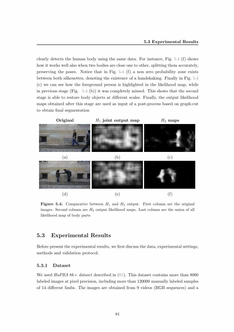
5.3 Experimental Results
clearly detects the human body using the same data. For instance, Fig. 5.4 (f) shows
how it works well also when two bodies are close one to other, splitting them accurately,
preserving the poses. Notice that in Fig. 5.4 (f) a non zero probability zone exists
between both silhouettes, denoting the existence of a handshaking. Finally in Fig. 5.4
(c) we can see how the foreground person is highlighted in the likelihood map, while
in previous stage (Fig. 5.4 (b)) it was completely missed. This shows that the second
stage is able to restore body objects at different scales. Finally, the output likelihood
maps obtained after this stage are used as input of a post-process based on graph-cut
to obtain final segmentation
Original H1 joint output map H2 maps
(a) (b) (c)
(d) (e) (f)
Figure 5.4: Comparative between H1 and H2 output. First column are the original
images. Second column are H2 output likelihood maps. Last column are the union of all
likelihood map of body parts
5.3 Experimental Results
Before present the experimental results, we first discuss the data, experimental settings,
methods and validation protocol.
5.3.1 Dataset
We used HuPBA 8k+ dataset described in (61). This dataset contains more than 8000
labeled images at pixel precision, including more than 120000 manually labeled samples
of 14 different limbs. The images are obtained from 9 videos (RGB sequences) and a
81
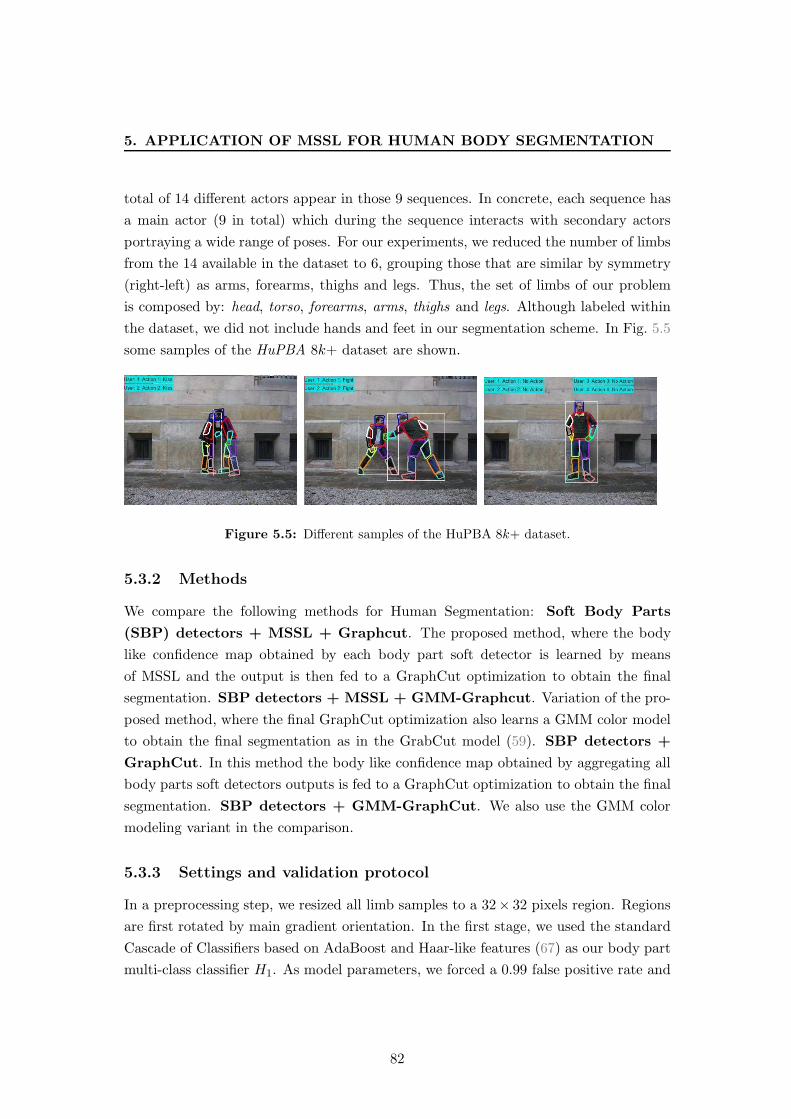
5. APPLICATION OF MSSL FOR HUMAN BODY SEGMENTATION
total of 14 different actors appear in those 9 sequences. In concrete, each sequence has
a main actor (9 in total) which during the sequence interacts with secondary actors
portraying a wide range of poses. For our experiments, we reduced the number of limbs
from the 14 available in the dataset to 6, grouping those that are similar by symmetry
(right-left) as arms, forearms, thighs and legs. Thus, the set of limbs of our problem
is composed by: head, torso, forearms, arms, thighs and legs. Although labeled within
the dataset, we did not include hands and feet in our segmentation scheme. In Fig. 5.5
some samples of the HuPBA 8k+ dataset are shown.
Figure 5.5: Different samples of the HuPBA 8k+ dataset.
5.3.2 Methods
We compare the following methods for Human Segmentation: Soft Body Parts
(SBP) detectors + MSSL + Graphcut. The proposed method, where the body
like confidence map obtained by each body part soft detector is learned by means
of MSSL and the output is then fed to a GraphCut optimization to obtain the final
segmentation. SBP detectors + MSSL + GMM-Graphcut. Variation of the pro-
posed method, where the final GraphCut optimization also learns a GMM color model
to obtain the final segmentation as in the GrabCut model (59). SBP detectors +
GraphCut. In this method the body like confidence map obtained by aggregating all
body parts soft detectors outputs is fed to a GraphCut optimization to obtain the final
segmentation. SBP detectors + GMM-GraphCut. We also use the GMM color
modeling variant in the comparison.
5.3.3 Settings and validation protocol
In a preprocessing step, we resized all limb samples to a 32× 32 pixels region. Regions
are first rotated by main gradient orientation. In the first stage, we used the standard
Cascade of Classifiers based on AdaBoost and Haar-like features (67) as our body part
multi-class classifier H1. As model parameters, we forced a 0.99 false positive rate and
82

5.3 Experimental Results
maximum of 0.4 false alarm rate during 8 stages. To detect limbs with trained cascades
of classifiers, we applied a sliding window approach with an initial patch size of 32× 32
pixels up to 60 × 60 pixels. As result of this stage, we obtained 6 likelihood maps for
each image. In the second stage, we performed 3-scale gaussian decomposition with σ ∈[8, 16, 32] for each body part. Then, we generated a extended set selecting for each pixel
its 8-neighbors with σ displacement. From this extended set, a sampling of 1500 selected
points formed the input examples for the second classifier. As second classifier, we used
a Random Forest with 50 decision trees. Finally, in a post-processing stage, binary
Graph Cuts with a GMM color modeling (we experimentally set 3 components) were
applied to obtain the binary segmentation where the initialization seeds of foreground
and background were tuned via cross-validation. For the binary Graph Cuts without
a GMM color modeling we directly fed the body likelihood map to the optimization
method. In order to assess our results, we used 9-fold cross-validation, where each fold
correspond to images of a main actor sequence. As results measurement we used the
Jaccard Index of overlapping (J = A⋂
BA⋃
B ) where A is the ground-truth and B is the
corresponding prediction.
5.3.4 Quantitative Results
In Table 5.1 we show overlapping results for the HuPBA 8K+ dataset. Specifically,
we show the mean overlapping value obtained by the compared methods on 9 folds of
the HuPBA 8k+ dataset. We can see how our MSSL proposal consistently obtains a
higher overlapping value on every fold.
Notice that MSSL proposal outperforms in the SBP+GC method in all folds (by at
least a 3% difference), which is the state-of-the-art method for human segmentation in
the HuPBA 8k+ dataset (60).
5.3.5 Qualitative Results
In Fig. 5.6 some qualitative results of the compared methodologies for human segmen-
tation are shown. It can be observed how in general SBP+MSSL+GMM-GC obtains
a better segmentation of the human body than the SBP + GMM-GC method. This
improvement is due to the contextual body part information encoded in the extended
feature set. In particular, this performance difference is clearly visible in Fig. 5.6(f)
where the human pose is completely extracted from the background. We also observe
how the proposed method is able to detect a significative number of body parts at dif-
ferent scales. This is clearly appreciated in Fig. 5.6(c), where persons at different scales
83
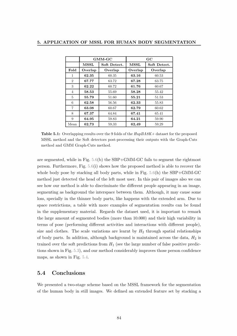
5. APPLICATION OF MSSL FOR HUMAN BODY SEGMENTATION
GMM-GC GC
MSSL Soft Detect. MSSL Soft Detect.
Fold Overlap Overlap Overlap Overlap
1 62.35 60.35 63.16 60.53
2 67.77 63.72 67.28 63.75
3 62.22 60.72 61.76 60.67
4 58.53 55.69 58.28 55.42
5 55.79 51.60 55.21 51.53
6 62.58 56.56 62.33 55.83
7 63.08 60.67 62.79 60.62
8 67.37 64.84 67.41 65.41
9 64.95 59.83 64.21 59.90
Mean 62,73 59,33 62,49 59,29
Table 5.1: Overlapping results over the 9 folds of the HupBA8K+ dataset for the proposed
MSSL method and the Soft detectors post-processing their outputs with the Graph-Cuts
method and GMM Graph-Cuts method.
are segmented, while in Fig. 5.6(b) the SBP+GMM-GC fails to segment the rightmost
person. Furthermore, Fig. 5.6(i) shows how the proposed method is able to recover the
whole body pose by stacking all body parts, while in Fig. 5.6(h) the SBP+GMM-GC
method just detected the head of the left most user. In this pair of images also we can
see how our method is able to discriminate the different people appearing in an image,
segmenting as background the interspace between them. Although, it may cause some
loss, specially in the thinner body parts, like happens with the extended arm. Due to
space restrictions, a table with more examples of segmentation results can be found
in the supplementary material. Regards the dataset used, it is important to remark
the large amount of segmented bodies (more than 10.000) and their high variability in
terms of pose (performing different activities and interactions with different people),
size and clothes. The scale variations are learnt by H2 through spatial relationships
of body parts. In addition, although background is maintained across the data, H2 is
trained over the soft predictions from H1 (see the large number of false positive predic-
tions shown in Fig. 5.3), and our method considerably improves those person confidence
maps, as shown in Fig. 5.4.
5.4 Conclusions
We presented a two-stage scheme based on the MSSL framework for the segmentation
of the human body in still images. We defined an extended feature set by stacking a
84

5.4 Conclusions
multi-scale decomposition of body part likelihood maps, which are learned by means of
a multi-class classifier based on soft body part detectors. The extended set of features
encodes spatial and contextual information of human limbs which combined enabled us
to define features with high order information. We tested our proposal on a large dataset
obtaining significant segmentation improvement over state-of-the-art methodologies.
85
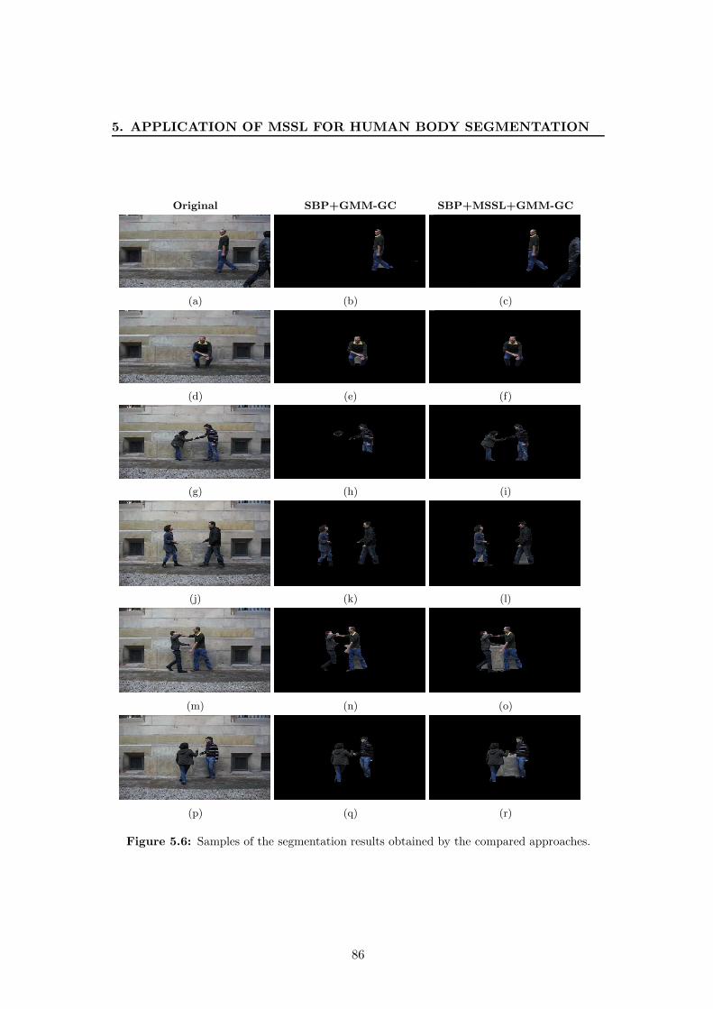
5. APPLICATION OF MSSL FOR HUMAN BODY SEGMENTATION
Original SBP+GMM-GC SBP+MSSL+GMM-GC
(a) (b) (c)
(d) (e) (f)
(g) (h) (i)
(j) (k) (l)
(m) (n) (o)
(p) (q) (r)
Figure 5.6: Samples of the segmentation results obtained by the compared approaches.
86

6
Conclusions
This thesis focuses on the problem of sequential learning from a meta-learning perspec-
tive.
Chapter 1 introduces the concept of sequential learning and the motivations of this
thesis.
Chapter 2 reviews some approaches of sequential learning from different points of
view. These approaches mainly comes from machine learning and pattern recognition
fields. However, since one of the motivations is to use sequential learning in images
classification tasks, we have reviewed some related works appeared in computer vision
field.
As a result of the research in this topic, in this thesis the following contributions
are proposed:
• In Chapter 3 we present a novel framework for sequential learning problems.
Specifically, we generalize the stacked sequential learning framework (SSL) stress-
ing the key role of the neighborhood modeling, in order to apply it in problems
such as object recognition or human body parts segmentation. Thanks to the
inclusion of function J after first classifier, where the multi-scale decomposition
and sampling of predictions is performed, our approach (MSSL) is more efficient
and capable to capture longer distance interactions than the original SSL. The
method allows to have an explicit trade-off between the resolution of the interac-
tions we desire to model and the number of features; very detailed interactions
can be modeled in short distance or long distance patterns can be captured with
a coarser resolution using the same number of features in the extended training
set. We show that strategies mixing detailed interactions and long ranges can be
defined at the cost of adding more features. The proposed method has been tested
87
6. CONCLUSIONS
on two different data sets, the first on a 1D correlation lattice and the second on
a 2D correlation lattice. We have compared our methodology with the graphical
model CRF. Our method has obtained better results in both datasets, assuming
non a priori knowledge of the structure of the labels. Even, our methodology is
more straight-forward than the graphical models, since the loss function depen-
dency is delegated to the base classifier. This means that the parametrization
of our method is only dependent on the base classifier, the number of scales in
the multi-resolution step and the number of sampled elements forming the ex-
tended data set. This last two parameters can be easily tuned depending on the
application dataset and the computation capacity available.
On going research in MSSL is towards to consider non-isotropic and/or non-linear
decomposition methods. Recently, Gatta and Ciompi (33) use scale-space Taylor
coefficients in order to model the neighborhood relationships, instead of using
multi-resolution decomposition. Meanwhile, we have already performed some
experiments applying wavelets and bilateral filters instead of multi-resolution de-
composition, but in the general case, the results have not been significantly better
than the ones obtained using MSSL.
• In Chapter 4 we develop some improvements over MSSL framework. Specifically,
we have developed a general and efficient extension of MSSL for the multi-class
case by integrating the ECOC framework in the base classifiers. We test our
multi-class methodology performing different experiments out from four databases
showing different kind of sequential relationships: Sensor motion data database,
FAQ database, IVUS image database and e-trims database. We test all the
databases with different configurations of our MSSL methodology, including a
feature-compression approach based on sub-lineal ECOCs. Finally, we compare
our results with Real Adaboost and CRF Multi-label optimization through Graph
Cut α-expansion methodologies.
As future work we going to experiment with other compression approaches, such
as compressed sensing or PCA, for the sake of reducing the extended set as much
as possible without losing accuracy.
• The last contribution of this chapter is an architecture specifically designed for
classification of different sized objects. The challenge in this problem comes by
the fact that the classifier has not been necessarily exposed to examples at the
different scales found in the testing images. We have used two images dataset for
testing our architecture: a data base of pictures of different sized horses and a
88

data base of different types and sized flowers. Adaboost and CRF are also used
as baseline experiments in order to compare our achieved results.
As future work we consider a scale and rotation invariant architecture, shifting
not only the scales but also the sampled neighborhood patterns.
• Finally, in Chapter 5 we present an application of MSSL for human body seg-
mentation. We presented a two-stage scheme based on the MSSL framework for
the segmentation of the human body in still images. We defined an extended
feature set based on likelihood maps obtained from soft body part detectors.
These features encode spatial and contextual information of human limbs provid-
ing high order information to the second classifier. We tested our proposal on a
large dataset obtaining significant segmentation improvement over state-of-the-
art methodologies.
Our work in progress is to refine our body segmentation application in order to
perform accurate multi-limb body segmentation. This is, to perform correctly
segmentation of each part of the body (arms, legs, torso, head...) by using our
MSSL framework.
89

6. CONCLUSIONS
90

Bibliography
[1] Aas, K., Eikvil, L. & Huseby, R. (1999). Applications of hidden markov chains
in image analysis. Pattern Recognition, 32, 703–713. 10
[2] Adelson, E.H., Anderson, C.H., Bergen, J.R., Burt, P.J. & Ogden, J.M.
(1984). Pyramid methods in image processing. RCA Engineer , 29, 33–41. 23
[3] Allwein, E., Schapire, R. & Singer, Y. (2002). Reducing multiclass to binary:
A unifying approach for margin classifiers. JMLR, 1, 113–141. 17, 48
[4] Andriluka, M., Roth, S. & Schiele, B. (2009). Pictorial structures revisited:
People detection and articulated pose estimation. In Computer Vision and Pattern
Recognition, 2009. CVPR 2009. IEEE Conference on, 1014–1021, IEEE. 76
[5] Bengio, Y. & Frasconi, P. (1996). Input-output HMM’s for sequence process-
ing. IEEE Transactions on Neural Networks, 7(5), 1231–1249. 13, 14
[6] Borenstein, E. & Malik, J. (2006). Shape guided object segmentation. In
CVPR (1), 969–976. 36
[7] Borenstein, E. & Ullman, S. (2002). Class-specific, top-down segmentation. In
Proceedings of the European Conference on Computer Vision, vol. 2351, 109–124,
Copenhagen, Denmark. 31, 32, 35, 36
[8] Borenstein, E. & Ullman, S. (2004). Learning to segment. In T. Pajdla &
J. Matas, eds., European Conference on Computer Vision (3), vol. 3023 of Lecture
Notes in Computer Science, 315–328, Springer. 54
[9] Bourdev, L., Maji, S., Brox, T. & Malik, J. (2010). Detecting people using
mutually consistent poselet activations. In Computer Vision–ECCV 2010 , 168–
181, Springer. 76
91

BIBLIOGRAPHY
[10] Boykov, Y. & Funka-Lea, G. (2006). Graph cuts and efficient nd image seg-
mentation. International Journal of Computer Vision, 70, 109–131. 58
[11] Boykov, Y., Veksler, O. & Zabih, R. (2001). Fast approximate energy mini-
mization via graph cuts. IEEE Trans. Pattern Anal. Mach. Intell., 23, 1222–1239.
16, 17
[12] Burt, P. & Adelson, E. (1983). The laplacian pyramid as a compact image
code. IEEE Transactions on Communications, 532–540. 21
[13] Cai, J. & Liu, Z. (2002). Pattern recognition using markov random field models.
Pattern Recognition, 35, 725–733. 14
[14] Casale, P., Pujol, O. & Radeva, P. (2012). Personalization and user verifi-
cation in wearable systems using biometric walking patterns. Personal Ubiquitous
Comput., 16, 563–580. 57
[15] Chakraborty, B., Bagdanov, A.D., Gonzalez, J. & Roca, X. (2011). Hu-
man action recognition using an ensemble of body-part detectors. Expert Systems.
75
[16] Ciompi, F., Pujol, O., Gatta, C., Carrillo, X., Mauri, J. & Radeva, P.
(2011). A holistic approach for the detection of media-adventitia border in ivus.
In MICCAI (3), 411–419. 58
[17] Cohen, W.W. & de Carvalho, V.R. (2005). Stacked sequential learning. Proc.
of IJCAI 2005 , 671–676. 2, 19, 27, 58
[18] Cour, T. & Shi, J. (2007). Recognizing objects by piecing together the segmen-
tation puzzle. In Proc. IEEE Computer Society Conference on Computer Vision
and Pattern Recognition, 1 – 8, IEEE Computer Society, Minneapolis, Minnesota,
USA. 16
[19] Dalal, N. & Triggs, B. (2005). Histograms of oriented gradients for human
detection. In CVPR, vol. 1, 886 –893. 58, 75
[20] Dantone, M., Gall, J., Leistner, C. & van Gool, L. (2013). Human pose
estimation using body parts dependent joint regressors. In Computer Vision and
Pattern Recognition (CVPR), 2013 IEEE Conference on, 3041–3048. 75
[21] Darroch, J.N. & Ratcliff, D. (1972). Generalized iterative scaling for log-
linear models. The Annals of Mathematical Statistics, 43, 1470–1480. 14
92
BIBLIOGRAPHY
[22] Dempster, A.P., Laird, N.M. & Rubin, D.B. (1977). Maximum likelihood
from incomplete data via the em algorithm. JOURNAL OF THE ROYAL STA-
TISTICAL SOCIETY, SERIES B , 39, 1–38. 14
[23] Demsar, J. (2006). Statistical comparisons of classifiers over multiple data sets.
J. Mach. Learn. Res., 7, 1–30. 33, 59, 63
[24] Dietterich, T. & Bakiri, G. (1995). Solving multiclass learning problems via
error-correcting output codes. In Journal of Artificial Intelligence Research, vol. 2,
263–286. 17, 48
[25] Dietterich, T.G. (2002). Machine learning for sequential data: A review. In
Proceedings of the Joint IAPR International Workshop on Structural, Syntactic,
and Statistical Pattern Recognition, 15–30, Springer-Verlag, London, UK. 1, 2, 8,
17
[26] Dietterich, T.G., Ashenfelter, A. & Bulatov, Y. (2004). Training condi-
tional random fields via gradient tree boosting. In Proceedings of the 21th Interna-
tional Conference on Machine Learning , 217–224, ACM, Banff, Alberta, Canada.
27, 58
[27] Escalera, S., Tax, D., Pujol, O., Radeva, P. & Duin, R. (2008). Subclass
problem-dependent design of error-correcting output codes. PAMI , 30, 1–14. 17,
48, 49
[28] Escalera, S., Pujol, O. & Radeva, P. (2010). On the decoding process in
ternary error-correcting output codes. PAMI , 32, 120–134. 49, 77
[29] Fawcett, T. & Provost, F. (1997). Adaptive fraud detection. Data Mining and
Knowledge Discovery , 1, 291–316. 9
[30] Felzenszwalb, P.F. & Huttenlocher, D.P. (2000). Efficient matching of pic-
torial structures. In Computer Vision and Pattern Recognition, 2000. Proceedings.
IEEE Conference on, vol. 2, 66–73, IEEE. 76
[31] Freund, Y. & Schapire, R. (1995). A decision-theoretic generalization of on-
line learning and an application to boosting. In EuroCOLT , 23–37. 58
[32] Friedman, J., Hastie, T. & Tibshirani, R. (2000). Additive Logistic Regres-
sion: a Statistical View of Boosting. The Annals of Statistics, 38. 46
93
BIBLIOGRAPHY
[33] Gatta, C. & Ciompi, F. (2014). Stacked sequential scale-space taylor context.
IEEE Transactions on Pattern Analysis and Machine Intelligence, 36, 1694–1700.
88
[34] Gatta, C., Puertas, E. & Pujol, O. (2011). Multi-scale stacked sequential
learning. Pattern Recognition, 44, 2414–2426. 4
[35] Gkioxari, G., Arbelaez, P., Bourdev, L.D. & Malik, J. (2013). Articu-
lated pose estimation using discriminative armlet classifiers. In CVPR, 3342–3349,
IEEE. 75
[36] Gorelick, L. & Basri, R. (2009). Shape based detection and top-down delin-
eation using image segments. Int. J. Comput. Vision, 83, 211–232. 16, 36
[37] Heitz, G. & Koller, D. (2008). Learning spatial context: Using stuff to find
things. In Proceedings of the 10th European Conference on Computer Vision, 30–
43, Springer-Verlag, Marseille, France. 16
[38] Hernandez-Vela, A., Reyes, M., Ponce, V. & Escalera, S. (2012).
Grabcut-based human segmentation in video sequences. Sensors, 12, 15376–15393.
76
[39] Hernandez-Vela, A., Zlateva, N., Marinov, A., Reyes, M., Radeva,
P., Dimov, D. & Escalera, S. (2012). Graph cuts optimization for multi-limb
human segmentation in depth maps. In CVPR, 726–732. 76
[40] Jaccard, P. (1901). Distribution de la flore alpine dans le bassin des drouces
et dans quelques regions voisines. Bulletin del la Societe Vaudoisedes Sciences
Naturelles, 37, 241–272. 32
[41] Korc, F. & Forstner, W. (2009). eTRIMS image database for interpreting
images of man-made scenes. Tech. Rep. TR-IGG-P-2009-01, Institute of Geodesy
and Geoinformation, Universitat Bonn. 58
[42] Kumar, M.P., Torr, P.H.S. & Zisserman, A. (2005). Obj cut. In Proceedings
of the 2005 IEEE Computer Society Conference on Computer Vision and Pat-
tern Recognition (CVPR’05) - Volume 1 - Volume 01 , CVPR ’05, 18–25, IEEE
Computer Society, Washington, DC, USA. 36
[43] Kumar, S. & Hebert, M. (2003). Discriminative random fields: A discriminative
framework for contextual interaction in classification. In Proceedings of the 2003
94
BIBLIOGRAPHY
IEEE International Conference on Computer Vision (ICCV ’03), vol. 2, 1150–
1157, Nice, France. 16
[44] Lafferty, J.D., McCallum, A. & Pereira, F. (2001). Conditional ran-
dom fields: Probabilistic models for segmenting and labeling sequence data.
In Proceedings of the International Conference on Machine Learning , 282–289,
Williamstown, MA, USA. 13, 14
[45] Lee, C.H., Greiner, R. & Schmidt, M.W. (2005). Support vector random
fields for spatial classification. In A. Jorge, L. Torgo, P. Brazdil, R. Camacho &
J. Gama, eds., PKDD , vol. 3721 of Lecture Notes in Computer Science, 121–132,
Springer. 57
[46] Levin, A. & Weiss, Y. (2009). Learning to combine bottom-up and top-down
segmentation. International Journal of Computer Vision, 81, 105–118. 36
[47] McCallum, A., Freitag, D. & Pereira, F.C.N. (2000). Maximum entropy
markov models for information extraction and segmentation. In Proceedings of
the Seventeenth International Conference on Machine Learning , 591–598, Morgan
Kaufmann Publishers Inc., San Francisco, CA, USA. 13, 28
[48] Mitchell, T.M. (1997). Machine Learning . McGraw-Hill, Inc., New York, NY,
USA, 1st edn. 7
[49] Nilsback, M.E. & Zisserman, A. (2006). A visual vocabulary for flower classi-
fication. In Proc. IEEE Conf. Comput. Vision Pattern Recog., vol. 2, 1447–1454,
IEEE Computer Society. 55
[50] Nilsson, N. (1965). Learning machines. In McGraw-Hill . 17, 49
[51] Pishchulin, L., Andriluka, M., Gehler, P. & Schiele, B. (2013). Pose-
let conditioned pictorial structures. In Computer Vision and Pattern Recognition
(CVPR), 2013 IEEE Conference on, 588–595, IEEE. 75, 76
[52] Puertas, E., Escalera, S. & Pujol, O. (2010). Classifying objects at different
sizes with multi-scale stacked sequential learning. In CCIA, 193–200. 5
[53] Puertas, E., Escalera, S. & Pujol, O. (2013). Generalized multi-scale stacked
sequential learning for multi-class classification. Pattern Analysis and Applica-
tions, 1–15. 5
95

BIBLIOGRAPHY
[54] Puertas, E., Bautista, M., S’anchez, D., Escalera, S. & Pujol, O.
(2014). Learning to segment humans by stacking their body parts. In ChaLearn
Looking at people Workshop, ECCV . 5
[55] Qian, N. & Sejnowski, T.J. (1988). Predicting the secondary structure of glob-
ular proteins using neural network models. Journal of Molecular Biology , 202,
865–884. 9
[56] Rabiner, L.R. (1989). A tutorial on hidden markov models and selected appli-
cations in speech recognition. Proceedings of the IEEE , 77, 257–286. 10, 12
[57] Ramanan, D., Forsyth, D. & Zisserman, A. (2005). Strike a pose: tracking
people by finding stylized poses. In Computer Vision and Pattern Recognition,
2005. CVPR 2005. IEEE Computer Society Conference on, vol. 1, 271–278 vol. 1.
75
[58] Ramanan, D., Forsyth, D. & Zisserman, A. (2007). Tracking people by learn-
ing their appearance. PAMI , 29, 65 –81. 75
[59] Rother, C., Kolmogorov, V. & Blake, A. (2004). ”grabcut”: interactive
foreground extraction using iterated graph cuts. ACM Trans. Graph., 23, 309–
314. 76, 82
[60] Sanchez, D., Ortega, J.C., Bautista, M.A. & Escalera, S. (2013). Human
body segmentation with multi-limb error-correcting output codes detection and
graph cuts optimization. In Proceedings of InPRIA, 50–58. 76, 77, 83
[61] Sanchez, D., Bautista, M. & Escalera, S. (2014). Hupba 8k+: Dataset and
ecocgraphcut based segmentation of human limbs. Neurocomputing . 81
[62] Sapp, B., Jordan, C. & Taskar, B. (2010). Adaptive pose priors for picto-
rial structures. In Computer Vision and Pattern Recognition (CVPR), 2010 IEEE
Conference on, 422–429, IEEE. 76
[63] Sejnowski, T.J. & Rosenberg, C.R. (1987). Parallel networks that learn to
pronounce english text. Complex Systems, 1, 145–168. 9
[64] Shotton, J., Fitzgibbon, A., Cook, M., Sharp, T., Finocchio, M.,
Moore, R., Kipman, A. & Blake, A. (2011). Real-Time Human Pose Recog-
nition in Parts from Single Depth Images. In Computer Vision and Pattern Recog-
nition. 80
96
BIBLIOGRAPHY
[65] Torralba, A. (2003). Contextual priming for object detection. Int. J. Comput.
Vision, 53, 169–191. 17
[66] Vineet, V., Warrell, J., Ladicky, L. & Torr, P. (2011). Human in-
stance segmentation from video using detector-based conditional random fields.
In BMVC . 76
[67] Viola, P. & Jones, M. (2001). Rapid object detection using a boosted cascade
of simple features. In CVPR, vol. 1. 75, 82
[68] Vishwanathan, S.V.N., Schraudolph, N.N., Schmidt, M.W. & Murphy,
K.P. (2006). Accelerated training of conditional random fields with stochastic
gradient methods. In Proceedings of the 23rd International Conference on Machine
Learning , 969–976, ACM, New York, NY, USA. 16, 31, 35
[69] Weiss, Y. (2001). Comparing the mean field method and belief propagation for
approximate inference in mrfs. 16
[70] Winn, J. (2005). Locus: Learning object classes with unsupervised segmentation.
In in ICCV , 756–763. 36
[71] Wolpert, D.H. (1992). Stacked generalization. Neural Networks, 241–259. 8, 10,
19
[72] Yang, Y. & Ramanan, D. (2011). Articulated pose estimation with flexible
mixtures-of-parts. In IEEE Conference on Computer Vision and Pattern Recogni-
tion, 1385–1392, IEEE. 76
[73] Yu, C.N.J. & Joachims, T. (2009). Learning structural svms with latent vari-
ables. In Proceedings of the 26th Annual International Conference on Machine
Learning , 1169–1176, ACM. 76
97