Embed Size (px)
Citation preview
Generalized Solovay Measures, the HOD Analysis, and the Core ModelInduction
by
Nam Duc Trang
A dissertation submitted in partial satisfaction of the
requirements for the degree of
Doctor of Philosophy
in
Mathematics
in the
Graduate Division
of the
University of California, Berkeley
Committee in charge:
Professor John Steel, ChairProfessor W. Hugh WoodinProfessor Sherrilyn Roush
Fall 2013
Generalized Solovay Measures, the HOD Analysis, and the Core ModelInduction
Copyright 2013by
Nam Duc Trang
1
Abstract
Generalized Solovay Measures, the HOD Analysis, and the Core Model Induction
by
Nam Duc Trang
Doctor of Philosophy in Mathematics
University of California, Berkeley
Professor John Steel, Chair
This thesis belongs to the field of descriptive inner model theory. Chapter 1 provides aproper context for this thesis and gives a brief introduction to the theory of AD+, the theoryof hod mice, and a definition of KJ(R). In Chapter 2, we explore the theory of generalizedSolovay measures. We prove structure theorems concerning canonical models of the theory“AD+ + there is a generalized Solovay measure” and compute the exact consistency strengthof this theory. We also give some applications relating generalized Solovay measures to thedeterminacy of a class of long games. In Chapter 3, we give a HOD analysis of AD+ + V =L(P(R)) models below “ADR + Θ is regular.” This is an application of the theory of hodmice developed in [23]. We also analyze HOD of AD+-models of the form V = L(R, µ)where µ is a generalized Solovay measure. In Chapter 4, we develop techniques for the coremodel induction. We use this to prove a characterization of AD+ in models of the formV = L(R, µ), where µ is a generalized Solovay measure. Using this framework, we also canconstruct models of “ADR + Θ is regular” from the theory “ZF + DC + Θ is regular + ω1 isP(R)-supercompact”. In fact, we succeed in going further, namely we can construct a modelof “ADR + Θ is measurable” and show that this is in fact, an equiconsistency.

i
To my parents
ii
Contents
List of Figures iv
1 Introduction 11.1 AD+ . . . . . . . . . . . . . . . . . . . . . . . . . . . . . . . . . . . . . . . . 31.2 Hod Mice . . . . . . . . . . . . . . . . . . . . . . . . . . . . . . . . . . . . . 51.3 A definition of KJ(R) . . . . . . . . . . . . . . . . . . . . . . . . . . . . . . 8
2 Generalized Solovay Measures 142.1 When α = 0 . . . . . . . . . . . . . . . . . . . . . . . . . . . . . . . . . . . . 18
2.1.1 The Equiconsistency . . . . . . . . . . . . . . . . . . . . . . . . . . . 182.1.2 Structure Theory . . . . . . . . . . . . . . . . . . . . . . . . . . . . . 21
2.2 When α > 0 . . . . . . . . . . . . . . . . . . . . . . . . . . . . . . . . . . . . 242.2.1 The Equiconsistency . . . . . . . . . . . . . . . . . . . . . . . . . . . 242.2.2 Structure Theory . . . . . . . . . . . . . . . . . . . . . . . . . . . . . 36
2.3 Applications . . . . . . . . . . . . . . . . . . . . . . . . . . . . . . . . . . . . 402.3.1 An Ultra-homogenous Ideal . . . . . . . . . . . . . . . . . . . . . . . 402.3.2 Determinacy of Long Games . . . . . . . . . . . . . . . . . . . . . . . 45
3 HOD Analysis 563.1 When V = L(P(R)) . . . . . . . . . . . . . . . . . . . . . . . . . . . . . . . 56
3.1.1 The Successor Case . . . . . . . . . . . . . . . . . . . . . . . . . . . . 563.1.2 The Limit Case . . . . . . . . . . . . . . . . . . . . . . . . . . . . . . 79
3.2 When V = L(R, µ) . . . . . . . . . . . . . . . . . . . . . . . . . . . . . . . . 863.2.1 HODL(R,µ) with M]
ω2 . . . . . . . . . . . . . . . . . . . . . . . . . . . 87
3.2.2 HODL(R,µ) without M]ω2 . . . . . . . . . . . . . . . . . . . . . . . . . 93
3.2.3 HODL(R,µα) for α > 0 . . . . . . . . . . . . . . . . . . . . . . . . . . . 95
4 The Core Model Induction 974.1 Framework for the Induction . . . . . . . . . . . . . . . . . . . . . . . . . . . 974.2 Θ > ω2 Can Imply AD+ . . . . . . . . . . . . . . . . . . . . . . . . . . . . . 100
4.2.1 Introduction . . . . . . . . . . . . . . . . . . . . . . . . . . . . . . . . 100
iii
4.2.2 Basic setup . . . . . . . . . . . . . . . . . . . . . . . . . . . . . . . . 1014.2.3 Getting one more Woodin . . . . . . . . . . . . . . . . . . . . . . . . 1024.2.4 ΘK(R) = Θ . . . . . . . . . . . . . . . . . . . . . . . . . . . . . . . . . 1064.2.5 An alternative method . . . . . . . . . . . . . . . . . . . . . . . . . . 1104.2.6 AD in L(R, µ) . . . . . . . . . . . . . . . . . . . . . . . . . . . . . . . 112
4.3 ZF + DC + Θ is regular + ω1 is P(R)-supercompact . . . . . . . . . . . . . 1154.3.1 Digression: upper bound for consistency strength . . . . . . . . . . . 1154.3.2 Θ > θ0 . . . . . . . . . . . . . . . . . . . . . . . . . . . . . . . . . . . 1194.3.3 ADR + Θ is regular . . . . . . . . . . . . . . . . . . . . . . . . . . . . 1204.3.4 ADR + Θ is measurable . . . . . . . . . . . . . . . . . . . . . . . . . . 128
Bibliography 142
iv
List of Figures
2.1 Implications in the proof of part 2 of Theorem 2.3.11 . . . . . . . . . . . . . 50
3.1 The process in Theorem 3.1.24 . . . . . . . . . . . . . . . . . . . . . . . . . . 733.2 The proof of branch condensation of Λ in Lemma 3.1.36 . . . . . . . . . . . . 85
4.1 The construction of Σ+σ . . . . . . . . . . . . . . . . . . . . . . . . . . . . . . 138
v
Acknowledgments
I would firstly like to thank my parents for the sacrifice they’ve made in order to give meand my brother a better future in the U.S. I would also like to thank my aunts, uncles,my grandparents in Vietnam who raised me, and my relatives in the U.S. who helped andsupported my family during the first few difficult years in a foreign country.
I would like to thank Grigor Sargsyan, who developed the theory of hod mice, for men-toring me. A large part of this thesis comes from countless conversations with him. I wouldalso like to thank my advisor, John Steel, for many discussions about descriptive inner modeltheory and for patiently correcting countless mistakes I’ve made over the years. The big pic-ture about descriptive set theory, inner model theory, and their connection that I’ve gainedcomes from those conversations. I would like to thank Hugh Woodin for developing thebeautiful theory of AD+ and the core model induction technique that most of this thesis re-volves about and for sharing with me his deep insight and knowledge in set theory. Withouthim, much of this thesis wouldn’t exist. Lastly, I thank Martin Zeman for introducing meto set theory.
1
Chapter 1
Introduction
In this chapter, we briefly discuss the the general subject of descriptive inner modeltheory, which provides the context for this thesis; we then summarize basic definitions andfacts from the theory of AD+, the theory of hod mice that we’ll need in this thesis, and adefinition of KJ(R) for certain mouse operators J .
Descriptive inner model theory (DIMT) is a crossroad between pure descriptive set theory(DST) and inner model theory (IMT) and as such it uses tools from both fields to study anddeepen the connection between canonical models of large cardinals and canonical models ofdeterminacy. The main results of this thesis are theorems of descriptive inner model theory.
The first topic this thesis is concerned with is the study of a class of measures calledgeneralized Solovay measures (defined in Chapter 2). In [28], Solovay defines a normal finemeasure µ0 on Pω1(R) from ADR. Martin and Woodin independently prove that determinacyof real games of fixed countable length follows from ADR and define a hierarchy of normalfine measures 〈µα | α < ω1〉, where each µα is on the set of increasing and continuous funtionsfrom ωα into Pω1(R) (this set is denoted Xα in Chapter 2). They also define the so-called“ultimate measure” µω1 on increasing and continuous functions from α (α < ω1) into Pω1(R)(this set is denoted Xω1 in Chapter 2) and prove the existence of µω1 from ADR, though notfrom determinacy of long games. The obvious question that arises is whether the consitencyof the theory (Tα) ≡ “AD + there is a normal fine measure on Xα” (for α ≤ ω1) implies theconsistency of the theory ADR. The answer is “no” and this follows from work of Solovay [28].Woodin shows furthermore that (T0) is equiconsistent with “ZFC + there are ω2 Woodincardinals”, which in turns is much weaker in consistency strength than ADR. This is theoriginal motivation of this investigation of generalized Solovay measures.
Generalizing Woodin’s above result, Chapter 2 computes the exact consistency strengthof “AD + there is a normal fine measure on Xα” for all α > 0 and shows that these theoriesare much weaker than ADR consistency-wise. Chapter 2 also contains various other resultsconcerning structure theory of AD+-models of the form V = L(R, µα), where µα is a normalfine measure on Xα (for α ≤ ω1) and its applications.
The second topic of this thesis is the HOD analysis. The HOD analysis is an integral
CHAPTER 1. INTRODUCTION 2
part of descriptive inner model theory as it is the key ingredient in the proof of the MouseSet Conjecture (MSC), which is an important conjecture that provides a connection betweencanonical models of large cardinals and canonical models of determinacy. We recall a bit ofhistory on the computation of HOD. Under AD, Solovay shows that HOD κ is measurablewhere κ = ωV1 . This suggests that HOD of canonical models of determinacy (like L(R)) is amodel of large cardinals. Martin and Steel in [16] essentially show that HODL(R) CH. Themethods used to prove the results above are purely descriptive set theoretic. Then Steel, (in[42] or [37]) using inner model theory, shows V HOD
Θ is a fine-structural premouse, which inparticular implies V HOD
Θ GCH. Woodin (see [31]), building on Steel’s work, completes thefull HOD analysis in L(R) and shows HOD GCH + Θ is Woodin and furthermore showsthat the full HOD of L(R) is a hybrid mouse that contains some information about a certainiteration strategy of its initial segments. A key fact used in the computation of HOD inL(R) is that if L(R) AD then L(R) MC1. It’s natural to ask whether analogous resultshold in the context of AD+ + V = L(P(R)). Recently, Grigor Sargsyan in [23], assumingV = L(P(R)) and there is no models of “ADR + Θ is regular” (we call this smallnessassumption (*) for now), proves Strong Mouse Capturing (SMC) (a generalization of MC)and computes V HOD
Θ for Θ being limit in the Solovay sequence and V HODθα
for Θ = θα+1 in asimilar sense as above.
Chapter 3 extends Sargsyan’s work to the computation of full HOD under (*). Thisanalysis heavily uses the theory of hod mice developed by Sargsyan in [23]. Chapter 3also computes full HOD of AD+-models of the form L(R, µα) as part of the analysis of thestructure theory of these models. This is used to prove (among other things) ADR,ωαΠ˜1
1
implies (and hence is equivalent to) ADR,ωα <-ω2-Π˜11 for 1 ≤ α < ω1 (I believe the case α = 1
has been known before).The last topic of this thesis concerns the core model induction (CMI). CMI is a powerful
technique of descriptive inner model theory pioneered by Woodin and further developedby Steel, Schindler, and others. It draws strength from natural theories such as PFA toinductively construct canonical models of determinacy and large cardinals in a locked-stepprocess. This thesis develops methods for the core model induction to solve a variety ofproblems. The first of which is a characterization of determinacy in models of the formL(R, µα) (α < ω1). I show that L(R, µα) AD if and only if L(R, µα) Θ > ω2 (see Section4.2). Another major application of the core model induction in this thesis is the proof of theequiconsistency of the theories: “ZF + DC + Θ is regular + ω1 is P(R)-supercompact” and“ADR + Θ is measurable” (see Section 4.3).
1MC stands for Mouse Capturing, which is the statement that if x, y ∈ R, then x ∈ OD(y) ⇔ x is in amouse over y.
CHAPTER 1. INTRODUCTION 3
1.1 AD+
We start with the definition of Woodin’s theory of AD+. In this thesis, we identify R withωω. We use Θ to denote the sup of ordinals α such that there is a surjection π : R→ α.
Definition 1.1.1. AD+ is the theory ZF + AD + DCR and
1. for every set of reals A, there are a set of ordinals S and a formula ϕ such thatx ∈ A⇔ L[S, x] ϕ[S, x]. (S, ϕ) is called an ∞-Borel code for A;
2. for every λ < Θ, for every continuous π : λω → ωω, for every A ⊆ R, the set π−1[A] isdetermined.
AD+ is arguably the right structural strengthening of AD. In fact, AD+ is equivalent to“AD + the set of Suslin cardinals is closed” (see [12]). Another, perhaps more useful,equivalence of AD+ is “AD + Σ1 statements reflect to Suslin-co-Suslin” (see [40] for a moreprecise statement).
Recall that Θ is defined to be the supremum of α such that there is a surjection fromR onto α. Under AC, Θ is just c
+. In the context of AD, Θ is shown to be the supremumof w(A)2 for A ⊆ R. Let A ⊆ R, we let θA be the supremum of all α such that there is anOD(A) surjection from R onto α.
Definition 1.1.2 (AD+). The Solovay sequence is the sequence 〈θα | α ≤ Ω〉 where
1. θ0 is the sup of ordinals β such that there is an OD surjection from R onto β;
2. if α > 0 is limit, then θα = supθβ | β < α;
3. if α = β + 1 and θβ < Θ (i.e. β < Ω), fixing a set A ⊆ R of Wadge rank θβ, θα is thesup of ordinals γ such that there is an OD(A) surjection from R onto γ, i.e. θα = θA.
Note that the definition of θα for α = β + 1 in Definition 1.1.2 does not depend on thechoice of A. We recall some basic notions from descriptive set theory.
Suppose A ⊆ R and (N,Σ) is such that N is a transitive model of “ZFC−Replacement”and Σ is an (ω1, ω1)-iteration strategy or just ω1-iteration strategy for N . We use o(N),ORN , ORDN interchangably to denote the ordinal height of N . Suppose that δ is countablein V but is an uncountable cardinal of N and suppose that T, U ∈ N are trees on ω× (δ+)N .We say (T, U) locally Suslin captures A at δ over N if for any α ≤ δ and for N -genericg ⊆ Coll(ω, α),
A ∩N [g] = p[T ]N [g] = RN [g]\p[U ]N [g].
2w(A) is the Wadge rank of A. We will use either w(A) or |A|w to denote the Wadge rank of A.
CHAPTER 1. INTRODUCTION 4
We also say that N locally Suslin captures A at δ. We say that N locally captures A ifN locally captures A at any uncountable cardinal of N . We say (N,Σ) Suslin captures Aat δ, or (N, δ,Σ) Suslin captures A, if there are trees T, U ∈ N on ω × (δ+)N such thatwhenever i : N → M comes from an iteration via Σ, (i(T ), i(U)) locally Suslin captures Aover M at i(δ). In this case we also say that (N, δ,Σ, T, U) Suslin captures A. We say (N,Σ)Suslin captures A if for every countable δ which is an uncountable cardinal of N , (N,Σ)Suslin captures A at δ. When δ is Woodin in N , one can perform genericity iterations onN to make various objects generic over an iterate of N . This is where the concept of Suslincapturing becomes interesting and useful. We’ll exploit this fact on several occasions.
Definition 1.1.3. Γ is a good pointclass if it is closed under recursive preimages, closedunder ∃R, is ω-parametrized, and has the scale property. Furthermore, if Γ is closed under∀R, then we say that Γ is inductive-like.
Under AD+, Σ12, Σ2
1 are examples of good poinclasses. If Γ is a good pointclass, we say(N,Σ) Suslin captures Γ if it Suslin captures every A ∈ Γ. The following are two importantstructure theorems of AD+ that are used at many places throughout this thesis.
Theorem 1.1.4 (Woodin, Theorem 10.3 of [35]). Assume AD+ and suppose Γ is a goodpointclass and is not the last good pointclass. There is then a function F defined on R suchthat for a Turing cone of x, F (x) = 〈N ∗x ,Mx, δx,Σx〉 such that
1. N ∗x |δx =Mx|δx,
2. N ∗x “ZF + δx is the only Woodin cardinal”,
3. Σx is the unique iteration strategy of Mx,
4. N ∗x = L(Mx,Λ) where Λ is the restriction of Σx to stacks ~T ∈ Mx that have finitelength and are based on Mx δx,
5. (N ∗x ,Σx) Suslin captures Γ,
6. for any α < δx and for any N ∗x -generic g ⊆ Coll(ω, α), (N ∗x [g],Σx) Suslin capturesCode((Σx)Mxα) and its complement at δ+
x .
Theorem 1.1.5 (Woodin, unpublished but see [40]). Assume AD+ +V = L(P(R)). SupposeA is a set of reals such that there is a Suslin cardinal in the interval (w(A), θA). Then
1. The pointclass Σ21˜(A) has the scale property.
2. M∆˜21(A) ≺Σ1 L(P(R)).
3. LΘ(P(R)) ≺Σ1 L(P(R)).
Finally, we quote another theorem of Woodin, which will be key in our HOD analysis.
Theorem 1.1.6 (Woodin, see [13]). Assume AD+. Let 〈θα | α ≤ Ω〉 be the Solovay sequence.Suppose α = 0 or α = β + 1 for some β < Ω. Then HOD θα is Woodin.
CHAPTER 1. INTRODUCTION 5
1.2 Hod Mice
In this subsection, we summarize some definitions and facts about hod mice that will be usedin our computation. For basic definitions and notations that we omit, see [23]. The formaldefinition of a hod premouse P is given in Definition 2.12 of [23]. Let us mention some basicfirst-order properties of P . There are an ordinal λP and sequences 〈(P(α),ΣPα ) | α < λP〉and 〈δPα | α ≤ λP〉 such that
1. 〈δPα | α ≤ λP〉 is increasing and continuous and if α is a successor ordinal then P δPαis Woodin;
2. P(0) = Lpω(P|δ0)P ; for α < λP , P(α + 1) = (LpΣPαω (P|δα))P ; for limit α ≤ λP ,
P(α) = (Lp⊕β<αΣPβω (P|δα))P ;
3. P ΣPα is a (ω, o(P), o(P))3-strategy for P(α) with hull condensation;
4. if α < β < λP then ΣPβ extends ΣPα .
We will write δP for δPλP and ΣP = ⊕β<λPΣPβ+1.
Definition 1.2.1. (P ,Σ) is a hod pair if P is a countable hod premouse and Σ is a (ω, ω1, ω1)iteration strategy for P with hull condensation such that ΣP ⊆ Σ and this fact is preservedby Σ-iterations.
Hod pairs typically arise in AD+-models, where ω1-iterability implies ω1 + 1-iterability.In practice, we work with hod pairs (P ,Σ) such that Σ also has branch condensation.
Theorem 1.2.2 (Sargsyan). Suppose (P ,Σ) is a hod pair such that Σ has branch conden-sation. Then Σ is pullback consistent, positional and commuting.
The proof of Theorem 1.2.2 can be found in [23]. Such hod pairs are particularly impor-tant for our computation as they are points in the direct limit system giving rise to HOD.For hod pairs (MΣ,Σ), if Σ is a strategy with branch condensation and ~T is a stack onMΣ
with last model N , ΣN ,~T is independent of ~T . Therefore, later on we will omit the subscript~T from ΣN,~T whenever Σ is a strategy with branch condensation and MΣ is a hod mouse.
Definition 1.2.3. Suppose P and Q are two hod premice. Then P Ehod Q if there is α ≤ λQ
such that P = Q(α).
If P and Q are hod premice such that P Ehod Q then we say P is a hod initial segmentof Q. If (P ,Σ) is a hod pair, and Q Ehod P , say Q = P(α), then we let ΣQ be the strategyof Q given by Σ. Note that ΣQ ∩ P = ΣPα ∈ P .
3This just means ΣPα acts on all stacks of ω-maximal, normal trees in P.
CHAPTER 1. INTRODUCTION 6
All hod pairs (P ,Σ) have the property that Σ has hull condensation and therefore, micerelative to Σ make sense. To state the Strong Mouse Capturing we need to introduce thenotion of Γ-fullness preservation. We fix some reasonable coding (we call Code) of (ω, ω1, ω1)-
strategies by sets of reals. Suppose (P ,Σ) is a hod pair. Let I(P ,Σ) be the set (Q,ΣQ, ~T )
such that ~T is according to Σ such that i~T exists and Q is the end model of ~T and ΣQ is
the ~T -tail of Σ. Let B(P ,Σ) be the set (Q,ΣQ, ~T ) such that there is some R such that
Q = R(α), ΣQ = ΣR(α) for some α < λR and (R,ΣR, ~T ) ∈ I(P ,Σ).
Definition 1.2.4. Suppose Σ is an iteration strategy with hull-condensation, a is a countabletransitive set such that MΣ ∈ a4 and Γ is a pointclass closed under boolean operations andcontinuous images and preimages. Then LpΓ,Σ
ω1(a) = ∪α<ω1Lp
Γ,Σα (a) where
1. LpΓ,Σ0 (a) = a ∪ a
2. LpΓ,Σα+1(a) = ∪M :M is a sound Σ-mouse over LpΓ,Σ
α (a)5 projecting to LpΓ,Σα (a) and
having an iteration strategy in Γ.
3. LpΓ,Σλ (a) = ∪α<λLpΓ,Σ
α (a) for limit λ.
We let LpΓ,Σ(a) = LpΓ,Σ1 (a).
Definition 1.2.5 (Γ-Fullness preservation). Suppose (P ,Σ) is a hod pair and Γ is a point-class closed under boolean operations and continuous images and preimages. Then Σ is aΓ-fullness preserving if whenever (~T ,Q) ∈ I(P ,Σ), α + 1 ≤ λQ and η > δα is a strongcutpoint of Q(α + 1), then
Q|(η+)Q(α+1) = LpΓ,ΣQ(α),~T (Q|η).
and
Q|(δ+α )Q = LpΓ,⊕β<αΣQ(β+1),~T (Q|δQα ).
When Γ = P(R), we simply say fullness preservation. A stronger notion of Γ-fullnesspreservation is super Γ-fullness preservation. Similarly, when Γ = P(R), we simply say superfullness preservation.
Definition 1.2.6 (Super Γ-fullness preserving). Suppose (P ,Σ) is a hod pair and Γ is apointclass closed under boolean operations and continuous images and preimages. Σ is superΓ-fullness preserving if it is Γ-fullness preserving and whenever (~T ,Q) ∈ I(P ,Σ), α < λQ
and x ∈ HC is generic over Q, then
LpΓ,ΣQ(α)(x) = M | Q[x] “M is a sound ΣQ(α)-mouse over x and ρω(M) = x”.4MΣ is the structure that Σ-iterates.5By this we mean M has a unique (ω, ω1 + 1)-iteration strategy Λ above LpΓ,Σ
α (a) such that wheneverN is a Λ-iterate of M, then N is a Σ-premouse.
CHAPTER 1. INTRODUCTION 7
Moreover, for such an M as above, letting Λ be the unique strategy for M, then for anycardinal κ of Q[x], Λ HQ[x]
κ ∈ Q[x].
Hod mice that go into the direct limit system that gives rise to HOD have strategies thatare super fullness preserving. Here is the statement of the strong mouse capturing.
Definition 1.2.7 (The Strong Mouse Capturing). The Strong Mouse Capturing (SMC) isthe statement: Suppose (P ,Σ) is a hod pair such that Σ has branch condensation and isΓ-fullness preserving for some Γ. Then for any x, y ∈ R, x ∈ ODΣ(y) iff x is in someΣ-mouse over 〈P , y〉.
When (P ,Σ) = ∅ in the statement of Definition 1.2.7 we get the ordinary Mouse Captur-ing (MC). The Strong Mouse Set Conjecture (SMSC) just conjectures that SMC holds belowa superstrong.
Definition 1.2.8 (Strong Mouse Set Conjecture). Assume AD+ and that there is no mousewith a superstrong cardinal. Then SMC holds.
Recall that by results of [23], SMSC holds assuming (*). To prove that hod pairs exist inAD+ models, we typically do a hod pair construction. For the details of this construction,see Definitions 2.1.8 and 2.2.5 in [23]. We recall the Γ-hod pair construction from [23] whichis crucial for our HOD analysis. Suppose Γ is a pointclass closed under complements andunder continuous preimages. Suppose also that λP is limit. We let
Γ(P ,Σ) = A | ∃(Q,ΣQ, ~T ) ∈ B(P ,Σ) A <w6Code(ΣQ).
HP Γ = (P ,Λ) | (P ,Λ) is a hod pair and Code(Λ) ∈ Γ,
and
MiceΓ = (a,Λ,M) | a ∈ HC, a is self-wellordered transitive, Λ is an iteration
strategy such that (MΛ,Λ) ∈ HP Γ, MΛ ∈ a, and M E LpΓ,Λ(a).
If Γ = P(R), we let HP = HP Γ and Mice = MiceΓ. Suppose (MΣ,Σ) ∈ HP Γ. Let
MiceΓΣ = (a,M) | (a,Σ,M) ∈MiceΓ.
Definition 1.2.9 (Γ-hod pair construction). Let Γ be an inductive-like pointclass and AΓ
be a universal Γ-set. Suppose (M, δ,Σ) is such that M ZFC - Replacement, (M, δ) iscountable, δ is an uncountable cardinal in M , Σ is an (ω1, ω1)-iteration strategy for M ,Σ∩(L1(Vδ))
M ∈M . Suppose M locally Suslin captures AΓ. Then the Γ-hod pair constructionof M below δ is a sequence 〈〈N β
ξ | ξ < δ〉,Pβ,Σβ, δβ | β ≤ Ω〉 that satisfies the followingproperties.
6Wadge reducible to
CHAPTER 1. INTRODUCTION 8
1. M Col(ω,<δ) “for all β < Ω, (Pβ,Σβ) is a hod pair such that Σβ ∈ Γ”7;
2. 〈N 0ξ | ξ < δ〉 are the models of the L[ ~E]-construction of V M
δ and 〈N βξ | ξ < δ〉 are
the models of the L[ ~E,Σβ]-construction of V Mδ . δ0 is the least γ such that o(N 0
γ ) = γand LpΓ(N 0
γ ) “γ is Woodin” and δβ+1 is the least γ such that o(N β+1γ ) = γ and
LpΓ,Σβ(N β+1γ ) “γ is Woodin”.
3. P0 = LpΓω(N 0
δ0) and Σ0 is the canonical strategy of P0 induced by Σ.
4. Suppose δβ+1 exists, N β+1δβ+1
doesn’t project across δβ. Furthermore, if β = 0 or is
successor and N β+1δβ+1 “δβ is Woodin” and if β is limit then (δ+
β )Pβ = (δ+β )Nβ+1δβ+1 , then
Pβ+1 = LpΓ,Σβω (N β+1
δβ+1) and Σβ+1 is the canonical strategy Pβ+1 induced by Σ.
5. For limit ordinals β, letting P∗β = ∪γ<βPγ, Σ∗β = γ<βΣγ, and δβ = supγ<βδγ, if δβ < δ
then let 〈N ∗,βξ | ξ < δ〉 be the models of the L[ ~E,Σ∗β]-construction of V Mδ . If there isn’t
any γ such that o(N ∗,βγ ) = γ and LpΓ,Σ∗β(N ∗,βγ ) “γ is Woodin” then we let Pβ be
undefined. Otherwise, let γ be the least such that o(N ∗,βγ ) = γ and LpΓ,Σ∗β(N ∗,βγ ) “γ
is Woodin.” If N ∗,βγ doesn’t project across δβ then Pβ = N ∗,βγ |(δ+ωβ )N
∗,βγ , and Σβ is the
canonical iteration strategy for Pβ induced by Σ. Otherwise, let Pβ be undefined.
1.3 A definition of KJ(R)
Definition 1.3.1. Let L0 be the language of set theory expanded by unary predicate symbolsE, B, S, and constant symbols l and a. Let a be a given transitive set. A model withparamemter a is an L0-structure of the form
M = (M ;∈, E,B,S, l, a)
such that M is a transtive rud-closed set containing a, the structureM is amenable, aM = a,S is a sequence of models with paramemter a such that letting Sξ be the universe of Sξ
• SSξ = S ξ for all ξ ∈ dom(S) and SSξ ∈ Sξ if ξ is a successor ordinal;
• Sξ = ∪α<ξSα for all limit ξ ∈ dom(S);
• if dom(S) is a limit ordinal then M = ∪α∈dom(S)Sα and l = 0, and
• if dom(S) is a successor ordinal, then dom(S) = l.
7This means there is a strategy Ψ for Pβ extending Σβ such that Code(Ψ) ∈ Γ and Ψ is locally Suslincaptured by M (at δ).
CHAPTER 1. INTRODUCTION 9
The above definition is due to Steel and comes from [46]. Typically, the predicate Ecodes the top extender of the model; S records the sequence of models being built so far.Next, we write down some notations regarding the above definition.
Definition 1.3.2. Let M be the model with parameter a. Then |M| denotes the universeof M. We let l(M) = dom(SM) denote the length of M and set M|ξ = SMξ for allξ < l(M). We set M|l(M) =M. We also let ρ(M) ≤ l(M) be the least such that there issome A ⊆M definable (from parameters in M) over M such that A ∩ |M|ρ(M)| /∈M .
Suppose J is a mouse operator that condenses well and relivizes well (in the sense of[26]). The definition of MJ,]
1 (more generally, the definition of a J-premouse over a self-wellorderable set) has been given in [26] and [46]. Here we only re-stratify its levels so as tosuit our purposes.
Definition 1.3.3. LetM be a model with parameter a, where a is self-wellorderable. SupposeJ is an iteration strategy for a mouse P coded in a. Let A be a set of ordinals coding thecofinal branch of T according to J , where T is the least (in the canonical well-ordering ofM) such that J(T ) /∈ |M| if such a tree exists; otherwise, let A = ∅. In the case A 6= ∅, letA∗ = o(M) + α | α ∈ A and ξ be
1. the least such that Jξ(M)[A∗] is a Q-structure of M|ρ(M) if such a ξ exists; or,
2. ξ is the least such that Jξ(M)[A∗] defines a set not amenable to M|ρ(M) if such a ξexists; or else,
3. ξ = sup(A∗).
For α ≤ ξ, we define Mα. For α = 0, let M0 =M. For 0 < α < ξ, suppose Mα has beendefined, we let
Mα+1 = (|J (Mα)[A∗]|;∈, ∅, A∗ ∩ |J (Mα)[A∗]|, SaMα, l(Mα) + 1, a).
For limit α, let Mα = ∪β<αMβ. We then let FJ(M) =Mξ. In the case A = ∅, we let
FJ(M) = (|J (M)|;∈, ∅, ∅, SaM, l(M) + 1, a).
In the case J is a (hybrid) first-order mouse operator8, we let J∗(M) be the least level ofJ(M) that is a Q-structure or defines a set not amenable to M|ρ(M) if it exists; other-wise, J∗(M) = J(M). We then define FJ(M) as follows. Let M0 = M. Suppose for αsuch that ωα < o(J∗(M)), we’ve defined M||α and maintained that |M||α| = |J∗(M)||α|,let Mα+1 = (|J∗(M)||(α + 1)|;∈, ∅, ∅, SaMα, l(Mα) + 1, a), where S = SMα. If α islimit and J∗(M)||α is passive, let Mα = ∪β<αMβ; otherwise, let Mα = (∪β<α|Mβ|;∈, E, ∅,∪β<αSMβ , supβ<αl(Mβ), a), where E is F
J∗(M)α . Finally,
8This means there is a (hybrid) mouse operator J ′ that condenses well such that there is a formula ψin the language of J ′-premice and some parameter a such that for every x ∈ dom(J), J(x) is the leastM LpJ
′(x) that satisfies ψ[x, a].
CHAPTER 1. INTRODUCTION 10
FJ(M) = Mγ, where ωγ = o(J∗(M)).
The rest of the definition of a J-premouse over a self-wellorderable set a is as in [46]. Wenow wish to extend this definition to non self-wellorderable sets a, and in particular to R.For this, we need to assume that the following absoluteness property holds of the operatorJ . We then show that if J is a mouse strategy operator for a nice enough strategy, then itdoes hold.
Definition 1.3.4. We say J determines itself on generic extensions (relative to N =MJ,]1 )
iff there are formulas ϕ, ψ in the language of J-premice such that for any correct, non-dropping iterate P of N , via a countable iteration tree, any P-cardinal δ, any γ ∈ OR suchthat P|γ ϕ+“δ is Woodin”, and any g which is set-generic over P|γ, then (P|γ)[g] is closedunder J and J P [g] is defined over (P|γ)[g] by ψ. We say such a pair (ϕ, ψ) genericallydetermines J .
The model operators that we encounter in the core model induction condense well, rela-tivize well, and determine themselves on generic extensions.
Definition 1.3.5. We say a (hod) premouse M is reasonable iff under ZF + AD, Msatisfies the first-order properties which are consequences of (ω, ω1, ω1)-iterability, or underZFC,M satisfies the first-order properties which are consequences of (ω, ω1, ω1+1)-iterability.
The following lemma comes from [27].
Lemma 1.3.6. Let (P ,Σ) be such that either (a) P is a reasonable premouse and Σ is theunique normal OR-iteration strategy for P; or (b) P is a reasonable hod premouse, (P ,Σ)is a hod pair which is fullness preserving and has branch condensation. Assume that MΣ
1
exists and is fully iterable. Then Σ determines itself on generic extensions.
Let M be a transitive model of some fragment of set theory. Let G be the canonicalCol(ω,M)-name for the generic G ⊆ Col(ω,M) and xG be the canonical name for the realcoding (n,m) | G(n) ∈ G(m), where we identify G with the surjective function from ωonto M that G produces. Let Λ be the strategy for N = MJ,]
1 . Using the terminology of[23], we say a tree T on N via Λ is the tree for making M generically generic if the followingholds:
1. T (o(M) + 1) is a linear iteration tree obtained by iterating the first total measureof M and its images o(M) + 1 times.
2. For α ≥ o(M) + 1, ETα is the extender with least index in MTα such that there is a
condition p ∈ Col(ω,M) such that p xG does not satisfy an axiom involving ETαfrom the extender algebra Bδ, where δ is the Woodin cardinal of MT
α .
CHAPTER 1. INTRODUCTION 11
We denote such a tree TM . Note that TM ∈ V , T is nowhere dropping, and lh(TM) < |M |+.Also note that TM does not include the last branch. Given a formula ϕ, let T ϕM = TM λ,where λ is least such that either λ = lh(TM) or λ is a limit ordinal and there is P E Q(TM λ)such that M(TM λ) E P and P ϕ. Now suppose there is P N such that N|δN E Pand P ϕ. Let λ ≤ lh(T ϕM) be a limit. If λ < lh(T ϕM) let Qϕ(TM λ) = Q(M(TM λ)).Otherwise let Qϕ(TM λ) = P , where P is least such that M(TM λ) E P E MTM
Λ(TM λ) andP ϕ.
We’re ready to define J-premice over an arbitrary transitive set a. The idea that todefine a Σ-premouse (over an arbitrary set), it suffices to tell the model branches of treesthat make certain levels of the model generically generic comes from [23], where it’s used toreorganize hod mice in such a way that S-constructions work.
Definition 1.3.7. Suppose a is a transitive set coding MJ,]1 . Suppose (ϕ, ψ) generically
determines J . Let Λ be the strategy for MJ,]1 . We define F ∗J (a) to be a level of a model M
with parameter a with the following properties. There is α < l(M) such that M|α ZF. Letα be the least such and let ξ be the largest cardinal of M|α = Jα(a). Let λ ≤ lh(T ϕM|α) be alimit. Let
Pα,λ = Qϕ(TM|α λ).
Let B ⊆ o(Pα,λ) be the standard set coding Pα,λ. Let ωγ = o(Pα,λ). Let for β < l(M),
Aβ = o(M|β) + η | η ∈ B × (α, λ).
and define
FJ,α,λ(M|β) = J Aβγ (M|β)
if no levels of J Aγ (M|β) is a Q-structure for (M|β)|ρ(M|β) or projects across ρ(M|β);
otherwise, let FJ,α,λ(M|β) = J (M|β).9.SupposeM|β has been defined and there is a λ such that Pα,λ is defined, T ϕM|α λ ∈M|β,
but for no β′ < l(M|β), FJ,α,λ(M|β′) 6= J (M|β′), we let then M|ξ∗ = FJ,α,λ(M|β), whereξ∗ = l(FJ,α,λ(M|β)) for the least such λ.
We say that T ϕM|α|λ is taken care of in M if there is a β < l(M) such that FJ,α,λ(M|β)
M and FJ,α,λ(M|β) 6= J (M|β). SoM is the least such that for every limit λ ≤ lh(T ϕM|α),
T ϕM|α λ is taken care of in M.
Finally, let F ∗J (a) =M if no levels ofM projects across ξ. Otherwise, let F ∗J (a) =M|β,where β is the least such that ρω(M|β) < ξ.
9Technically, FJ,α,λ(M|β) is stratified as a model over a but we suppress the structure for brevity. SeeDefinition 1.3.3 for the stratification.
CHAPTER 1. INTRODUCTION 12
Definition 1.3.8 (Potential J-premouse over a). Let a be a transitive structure such that acontains a real coding N . We say that M is a potential J-premouse over a iff M is amodel with parameter a, and there is an ordinal λ and a increasing, closed sequence 〈ηα〉α≤λof ordinals, such that for each α ≤ λ, we have:
(a) if a is not a self-wellordered set, then η0 = 1 and M|1 = a; otherwise, either λ = 0 andM =M|η0 EMJ,]
1 or else M|η0 =MJ,]1 (in the sense of Definition 1.3.3),
(b) ηα ≤ l(M),
(c) if α + 1 < λ, then M|ηα+1 = F ∗J (M|ηα),
(d) if α + 1 = λ, then M E F ∗J (M|ηα),10
(e) ηλ = l(M),
(f) if η = ηα and EM|η 6= ∅ (and therefore α is a limit) then EM|η codes an extender Ethat coheres M|η and satisfies the obvious modifications of the premouse axioms (in thesense of Definition 2.2.1 of [46]) and E is a× γ-complete for all γ < crt(E)11.
We define projecta, standard parameters, solidity, soundness, cores as in section 2.2 of[46].
Definition 1.3.9. Suppose M is a potential J-premouse over a. Then we say that M is aJ-premouse over a if for all λ < l(M), M|λ is ω-sound.
Definition 1.3.10. SupposeM is a J-premouse over a. We say thatM is active if EM 6= ∅or BM 6= ∅. Otherwise, we say that M is passive.
Definition 1.3.11 (J-mouse). Let M, a be as in Definition 1.3.9. We say that N is aJ-mouse over a if ρω(N ) = a and whenever N ∗ is a countable transitive J-premouse oversome a∗ and there is an elementary embedding π : N ∗ → N such that π(a∗) = a, then N ∗ isω1 + 1-iterable12 and whenever R is an iterate of N ∗ via its unique iteration strategy, R isa J-premouse over a∗.
Suppose M is a J-premouse over a. We say that M is J-complete if M is closed underthe operator F ∗J . The following lemma is also from [27].
Lemma 1.3.12. Suppose M is a J-premouse over a and M is J-complete. Then M isclosed under J ; furthermore, for any set generic extension g of N , N [g] is closed under Jand in fact, J is uniformly definable over N [g] (i.e. there is a L0-formula φ that defines Jover any generic extension of N).
10We will also use Mη to denote M|η.11This means whenever 〈Xx | x ∈ a × γ〉 ∈ M|λ is such that Xx ∈ Eb for each x ∈ a × γ, where b is a
finite subset of lh(E), then ∩x∈aXx ∈ Eb12Sometimes we need more than just ω1 + 1-iterability. See Chapter 4.
CHAPTER 1. INTRODUCTION 13
If a in Definition 1.3.11 is Hω1 , then we define LpJ(R) to be the union of all J-miceN overa13. In core model induction applications, we typically have a pair (P ,Σ) where P is eithera hod premouse and Σ is P ’s strategy with branch condensation and is fullness preserving(relative to mice in some pointclass) or P is a sound (hybrid) premouse projecting to somecountable set a and Σ is the unique (normal) strategy for P . Lemma 1.3.6 shows that Σcondenses well and determines itself on generic extension in the sense defined above. We thendefine LpΣ(R)14 as above and use a core model induction to prove LpΣ(R) AD+. What’sneeded to prove this is the scales analysis of LpΣ(R) AD+ from the optimal hypothesissimilar to those used by Steel to analyze the pattern of scales in K(R).
13We’ll be also saying J-premouse over R when a = Hω114In this thesis, we use LpΣ(R) and KΣ(R) interchangably.
14
Chapter 2
Generalized Solovay Measures
We work under the theory ZF + DC unless stated otherwise. For each α < ω1, for eachf : α→ Pω1(R), f is nice if for all i, f(i) is coded by an element in f(i + 1) (we will abusenotation and write “f(i) ∈ f(i+ 1)”) and if i is limit, f(i) = ∪j<if(j). Let Xα be the set ofall nice f : ωα → Pω1(R). Also let Xω1 = f : α→ Pω1(R) | f is nice and α < ω1. For anyf : α→ Pω1(R), we let Rf = ∪β<αf(β).
Definition 2.0.13 (Fineness). For α ≤ ω1, µα is said to be fine if for any σ ∈ Pω1(R), theset of all g ∈ Xα such that σ ∈ g(0) has µα-measure one.
Definition 2.0.14 (Normality). For α < ω1, a measure µα on Xα is normal if
1. (Fodor’s property) For any F : Xα → Pω1(R) such that ∀∗µαfF (f) ⊆ f(0) ∧ F (f) 6= ∅,there is an x ∈ R such that ∀∗µαf(x ∈ F (f));
2. (Shift invariance) If X ∈ µα and β < ωα, then fβ | f ∈ X ∈ µα where fβ(i) =f(β + i).
For α = ω1, a measure µα on Xα is normal if (1)-(2) hold for µα and
3. (Idempotence) If A,B ∈ µα, then AaB = fag | f ∈ A ∧ g ∈ B ∧ fag ∈ Xα ∈ µα.
Note that condition (1) of normality is the generalization of the Fodor’s property in theZFC context. This is all that we can demand for the following reasons. For α = 0, in thecontext of DC, the exact statement of Fodor’s lemma reduces to countable completeness ofµ0 and this is not sufficient to prove, for example, Los’s theorem for ultraproducts using µ0.Suppose α > 0 and consider the function F such that F (f) = x ∈ R | x codes f(0). Therecan’t be an x ∈ R that codes f(0) for µα-measure one many f .
Here’s an easy lemma that characterizes (1) in terms of diagonal intersection. The proofof the lemma, which does not use the axiom of choice, is easy and we leave it to the reader.
Lemma 2.0.15 (ZF + DC). Fix α < ω1 and suppose µα is a fine measure on Xα. Thefollowing are equivalent:
CHAPTER 2. GENERALIZED SOLOVAY MEASURES 15
(a) For all 〈Ax | x ∈ R ∧ Ax ∈ µα〉, 4x∈R = f ∈ Xα | f ∈ ∩x∈f(0)Ax ∈ µα.
(b) ∀∗µαf (F (f) ⊆ f(0)→ ∃x∀∗µαf x ∈ F (f)).
We need the following (unpublished) theorem of Woodin, which proves the existence ofmodels of “AD+ + there is a normal fine measure on Xα” for α ≤ ω1 from AD+ + ADR. Acorollary of Theorem 2.0.16 is Theorem 2.0.17, a well-known theorem of Solovay (α = 0) andof Martin and Woodin (α > 0).
Theorem 2.0.16 (Woodin). Assume AD++ADR. Let A ⊆ R. There is a tuple (M, ~E, δ,Σ, τ)such that
1. ~E is a weakly coherent extender sequence on M in the sense that if F ∈ ~E and iF :M → Ult(M,F ) is the ultrapower map then M agrees with Ult(M,F ) up to lh(F );
2. ~E witnesses that δ is a measurable limit of Woodin cardinals in M ;
3. τ is a Col(ω, δ)-term in M and Σ is an iteration strategy for M such that if i : M → Nis an iteration map according to Σ, then for any g ⊆ Col(ω, i(δ)) generic over N ,A ∩N [g] = i(τ)g.
Theorem 2.0.17 (Martin,Woodin). Assume AD+ + ADR. Then for all α ≤ ω1, there is anormal fine measure µα on Xα.
Proof. We’ll use Theorem 2.0.16 to show there is a normal fine measure µω1 on Xω1 . Themeasures µα can be constructed from µω1 as follows. For any A ⊆ Xα,
A ∈ µα ⇔ f ∈ Xω1 | f α ∈ A ∈ µω1 .
We proceed to define µω1 . Let A ⊆ Xω1 . A ∈ µω1 if for all B ⊆ R coding A1, letting(MB, ~EB, δB,ΣB, τB) be as in Theorem 2.0.16 for B, g ⊆ Col(ω,< δB) be MB-generic, δα bethe αth-limit of Woodin cardinals in MB, then 〈RMB [gδα] | δα < δB〉2 ∈ (τA)g.
Lemma 2.0.18. µω1 is a normal fine measure on Xω1.
Proof. We first show µω1 is a measure. Suppose not. There is an A ⊆ Xω1 such that thereare B,C ⊆ R coding A and (MB, ~EB, δB,ΣB, τB), (MC , ~EC , δC ,ΣC , τC) as in Theorem 2.0.16for B and C respectively and
MB ∅ Col(ω,<δB) fG ∈ τA,
but
MC ∅ Col(ω,<δC) fG /∈ τA.
1The coding is so that if M captures B by τB , then M captures A by some τA.2From now on, we’ll denote this sequence fg.
CHAPTER 2. GENERALIZED SOLOVAY MEASURES 16
We will get a contradiction by a back-and-forth argument that produces iteration mapsi : MB → NB, j : MC → NC such that there are gB ⊆ Col(ω,< i(δB)) generic over NB,gC ⊆ Col(ω,< j(δC)) generic over NC such that fgB = fgC .
We informally describe the first ω steps of this process. Let 〈δn | n < ω〉 and 〈γn | n < ω〉be the first ω Woodin cardinals of MB and MC respectively. Let M0 = MB and N0 = MC .We first iterate M0 below δ0 to produce i0 : M0 → M1 and g0 ⊆ Col(ω, i0(δ0)) such thatN0|γ0 ∈ M1[g0]. We then iterate in the window [γ0, γ1) and produce j0 : N0 → N1 andh0 ⊆ Col(ω, j0(γ1)) such that M1[g0]|δ0 ∈ N1[h0]. In general, for all 0 < n < ω, weproduce in : Mn → Mn+1 in the window [in−1 · · · i0(δn−1), in−1 · · · i0(δn)) and gn ⊆Col(ω, in · · · i0(δn)) extending gn−1 such that Nn[h0, . . . , hn−1]|(jn−1 · · · j0(γn−1)) ∈Mn+1[gn] and then jn : Nn → Nn+1 in the window [jn−1 · · · j0(γn−1), jn−1 · · · j0(γn)),hn ⊆ Col(ω, jn · · · j0(γn)) extending hn−1 such that Mn+1[gn]|(in · · · i0(δn)) ∈ Ni+1[hn].Let Mω and Nω be the direct limits of the Mn’s and Nn’s respectively. Let 〈δωn | n ≤ ω〉 and〈γωn | n ≤ ω〉 be the first ω Woodins and their sup of Mω and Nω respectively. Then it’sclear from our construction that σ0 = Mω[gn]|δωn | n < ω = Nω[hn]|γωn | n < ω is thesymmetric reals at δωω of Mω and γωω of Nω. Let gω ⊆ Col(ω, δωω) be Mω generic realizing σ0 asthe symmetric reals and hω ⊆ Col(ω, γωω ) be Nω generic realizing σ0 as the symmetric reals.We then repeat the back-and-forth process described above using the next ω Woodins. Whenwe use up the Woodins on one side but not the other, we hit the measure of the measurableWoodin cardinal of the shorter side to create more Woodin cardinals and continue the back-and-forth process. The coiteration will stop successfully when we use up the Woodins onboth sides. It’s easy to see that this process stops successfully and we produce G on the Mside and H on the N side such that fG = fH . Contradiction.
It’s easy to see that µω1 is fine. To verify property (2) of normality, suppose X ∈ µω1 andα < ω1 is such that Xα =def fα | f ∈ X /∈ µω1 where fα(i) = f(α+ i). So there is B ⊆ Rcoding X,Xα such that letting (MB, ~EB, δB,ΣB, τB) be as in Theorem 2.0.16 for B, we have
Col(ω,< δB) MB fG ∈ τX ∧ fG /∈ τXα .
Let M0 = N0 = MB and run the back-and-forth argument as above to get a contradiction.The difference here is in the first ω steps of the coiteration: on the M0 side the iteration usesthe first ω Woodins of M0 and on the N0 side the iteration ignores the first ωα Woodins ofN0 and uses the ωα + ith Woodins of N0. The process stops successfully and results in theend models Mω1 and Nω1 , generics G for Mω1 and H for Nω1 such that fG = fαH . But thenMω1 [G] fG /∈ Xα while Nω1 [H] fαH = fG ∈ Xα. This is a contradiction.
To verify property (1) of normality, suppose F is such that X = f ∈ Xω1 | F (f) 6=∅ ∧ F (f) ⊆ f(0) ∈ µω1 but for all x ∈ R, Yx = f ∈ X | x ∈ F (f) /∈ µω1 . Let B ⊆ Rcode F,X, Yx | x ∈ R and let (MB, ~EB, δB,ΣB, τB) be as in Theorem 2.0.16 for B. Lettingg ⊆ Col(ω, δB) be generic over MB, we have
MB[g] fg ∈ τX ∧ ∀x ∈ RMB(fg /∈ τYx),
which means
CHAPTER 2. GENERALIZED SOLOVAY MEASURES 17
MB[g] F (fg) 6= ∅ ∧ F (fg) ⊆ fg(0) ∧ ∀x ∈ RMB(x /∈ F (fg)).
For each x ∈ fg(0), let Mx = MB[x] and gx ⊆ Col(ω,< δB) generic over MB[x] suchthat fg(0) = fgx(0); also, let M∅ = MB. Now use the back-and-forth argument above tocoiterate Mx | x ∈ fg(0) above the first ω Woodins of each model. The process terminatessuccessfully and produce for each x ∈ fg(0) a model M∞
x , a generic g∞x over M∞x (at the
measurable limit of Woodins of the model) such that
1. for all x, y ∈ fg(0), fg∞x = fg∞y ;
2. for all x ∈ fg(0), fg∞x (0) = fg(0);
3. for all x ∈ fg(0), x /∈ F (fg∞x ).
(1)-(3) imply F (fg∞x ) = 0 for any x ∈ fg(0). This is a contradiction.
To verify (3), suppose A,B ∈ µω1 and let (M, ~E, δ,Σ, τ) witness this. This means M isboth A-iterable and B-iterable via Σ and the term τ computes the terms τA and τB. Letg ⊆ Col(ω, δ) be M -generic and let f = fg. Hence f ∈ A. Now let i : M → N be theultrapower map via a measure on δ in M . By coiterating N above δ and M and using aback-and-forth argument similar to the above, we get an iterate P of N (above δ) such thatletting j : N → P be the iteration map, there is a generic h ⊆ Col(ω, j(i(δ))) over P suchthat h extends g and fh\fg ∈ B. This means fh ∈ AaB. Hence we finish verifying (3).
It’s not clear that under AD++ADR, the measure µω1 defined above is the unique measuresatisfying (1)-(3) of Definition 2.0.14. However AD+ + ADR implies that the measures µα(for α < ω1) are unique. AD+ + ADR implies µ0 is unique (see [47]) (we just need DCR forthe proof of the main theorem in [47] for showing µ0 is unique). To show uniqueness of µαfor α > 0, we need the following definition. We identify Pω1(R) with X0.
Definition 2.0.19. Fix 0 ≤ α < ω1. Suppose A ⊆ Xα. We say that A is a club3 if there isa function F : R<ω → R such that clα,F = A where
clα,F = f ∈ Xα | ∀β F ′′f(β)<ω ⊆ f(β) ∧ F ′′f(β)<ω ∈ f(β + 1)4.
Martin and Woodin actually proves that under AD+ + ADR, real games of length α forany α < ω1 are determined. Hence for any α < ω1, for any A ⊆ Xα, either A contains aclub or R\A contains a club. By the same arguments Solovay uses to prove µ0 is normalunder ADR, we have that if 〈Ax | Ax ⊆ Xα ∧ x ∈ R〉 is a sequence of clubs then the diagonalintersection
3For α = 0, the notion of a club is just the usual notion of club for subsets of Pω1(R). Again we confuse
X0 for Pω1(R).4Recall that this means that there is a real in f(β + 1) that codes an enumeration of F ′′f(β)<ω
CHAPTER 2. GENERALIZED SOLOVAY MEASURES 18
4xAx =def f ∈ Xα | f ∈ ∩x∈f(0)Ax
contains a club.We show µ1 is unique and the proof of the other cases is similar. So suppose A ∈ µ1. It’s
enough to show A contains a club, that is A contains cl1,F for some F as in Definition 4.3.27.It’s easy to check that the following is an equivalent definition of µ1. We say A ∈ µ1 if for allB ⊆ R coding A, letting (MB, ~EB, δB,ΣB, τB) be as in Theorem 2.0.16 for B except that ~EBwitnesses that δB is a limit of ω2 Woodin cardinals in MB, g ⊆ Col(ω, δB) be MB-generic,
fg ∈ (τA)g. Fix an (MA, ~EA, δA,ΣA, τA). Then for a club of σ ∈ Pω1(R), σ is closed underΣA. Let F be such that for all σ ∈ Pω1(R) closed under F , σ is closed under ΣA. Usinggenericity iteration, it’s easy to see that for all f ∈ cl1,F , f ∈ A. This shows that wheneverA ∈ µ1, then A contains a club. Hence µ1 is the unique normal fine measure on X1, since itis just the club filter on X1. A similar proof works for 2 ≤ α < ω1.
2.1 When α = 0
2.1.1 The Equiconsistency
We assume familiarity with stationary tower forcing (see [14]) which will be used in the proofof the following theorem of Woodin.
Theorem 2.1.1 (Woodin). The following are equiconsistent.
1. ZFC + there are ω2 Woodin cardinals.
2. There is a filter µ on Pω1(R) such that L(R, µ) ZF + DC + AD + µ is a normal finemeasure on Pω1(R).
We first prove the (1)⇒ (2) direction of Theorem 2.1.1. Assume γ is the sup of ω2 Woodincardinals and for each i < ω, let ηi be the sup of the first ωi Woodin cardinals. SupposeG ⊆ Col(ω,< γ) is V -generic and for each i, let R∗ = ∪α<γRV [Gα] and σi = RV [GCol(ω,<ηi)].We define a filter F∗ as follows: for each A ⊆ R∗ in V [G]
A ∈ F∗ ⇔ ∃n∀m ≥ n(σm ∈ A).
We call F∗ defined above the tail filter .
Lemma 2.1.2. L(R∗,F∗) F∗ is a normal fine measure on Pω1(R∗).
Proof. Suppose not. So this statement is forced by the empty condition in Col(ω,< γ).
Claim. There is a forcing P of size less than the first Woodin cardinal such that in V P,L(R, C) “C is a normal fine measure on Pω1(R)” where C is the club filter on Pω1(R).
CHAPTER 2. GENERALIZED SOLOVAY MEASURES 19
Proof. Let κ be the first measurable cardinal and U be a normal measure on κ. Let j :V → M be the ultrapower map by U . Let P0 be Col(ω,< κ). Let G ⊆ P0 be V -generic.Col(ω,< j(κ)) = j(P0) is isomorphic to P0∗Q for some Q and whenever H ⊆ Q is V [G]-generic, then j can be lifted to an elementary embedding j+ : V [G] → M [G][H] defined byj+(τG) = j(τ)G∗H . We define a filter F∗ as follows.
A ∈ F∗ ⇔ ∀H ⊆ Q(H is V [G]-generic⇒ RV [G] ∈ j+(A)).
It’s clear from the definition that F∗ ∈ V [G]. Let R∗ = RV [G] is the symmetric reals. Weclaim that L(R∗,F∗) F∗ is a normal fine measure on Pω1(R)∗. Suppose A ∈ L(R∗,F∗) isdefined in V [G] by a formula ϕ from a real x ∈ R∗ (without loss of generality, we suppressparameters U, s, where s ∈ OR<ω that go into the definition of A); so σ ∈ A ⇔ V [G] ϕ[σ, x]. Let α < κ be such that x ∈ V [G α] and we let U∗ be the canonical extension of Uin V [G α]. Then either ∀∗U∗βV [G α] ∅ Col(ω,<β) ϕ[R, x] or ∀∗U∗βV [G α] ∅ Col(ω,<β)
¬ϕ[R, x]. This easily implies either A ∈ F∗ or ¬A ∈ F∗. We leave the proof of normalityand fineness to the reader.
Since PR∗ has size ω1 in V [G], we can then let P1 be the iterated club shooting posetdefined in 17.2 of [4] to shoot clubs through stationary subsets of PR∗ . By 17.2 of [4], P1
does not add any ω-sequence of ordinals. Letting H ⊆ P1 be V [G]-generic, in V [G][H], westill have L(R∗,F∗) F∗ is a normal fine measure on Pω1(R)∗ and furthermore, F is therestriction of the club filter on L(R∗,F∗). Our desirable P is P0∗P1.
By the claim, we may assume that in V , the club filter F on Pω1(R) has the propertythat L(R,F) F is a normal fine measure on Pω1(R). Let λ > γ be inaccessible and let
S = X ≺ Vλ | X is countable, γ ∈ X, ∃η ∈ X ∩ γ such that
for all successor Woodin cardinals λ ∈ X ∩ (η, γ), if D ⊆ Q<λ, D ∈ Xis predense then X captures D.
By lemma 3.1.14 of [14], S is stationary and furthermore, letting H ⊆ P(Pω1(Vλ))/INS begeneric such that S ∈ H, then for some ξ < γ, for all ξ < δ < γ and δ is Woodin, H ∩Q<δ
is V -generic. We may as well assume ξ is less than the first Woodin cardinal and hence forall δ < γ, δ is Woodin, H ∩Q<δ is V -generic.
Let j : V → (M,E) be the induced generic embedding given by H. Of course, (M,E)may not be wellfounded but wellfounded at least up to λ because j′′λ ∈M . For each α < ω2,let jα : V → Mα be the induced embedding by H ∩ Q<δα , let M∗ be the direct limit of theMα’s and j∗ : V →M∗ be the direct limit map. Note that jα, j
∗ factor into j.Let R∗ = RM∗ and for each i < ω, σi = RM∗i where M∗
i = limnMωi+n. Let G ⊆ Col(ω,<γ) be such that ∪α<ηiRV [Gα] = σi for all i. Let F∗ be the tail filter defined in V [G]. We claimthat if A ∈ j∗(F) then A ∈ F∗. To see this, let π ∈M∗ witness that A is a club. Let α < ω2
be such that Mα contains the preimage of π. Then it is clear that ∀m such that ωm ≥ αand π′′σm ⊆ σm. This shows j∗(F) ⊆ F∗ and hence Lλ(R∗, j∗(F)) = Lλ(R∗,F∗) F∗ is anormal fine measure on Pω1(R∗). Since λ can be chosen arbitrarily large, we’re done.
CHAPTER 2. GENERALIZED SOLOVAY MEASURES 20
Lemma 2.1.3. L(R∗,F∗) AD+.
Proof. We use the notation of Lemma 4.4. Note that from the proof of Theorem 4.4,L(R∗,F∗) = L(R∗,F) where F is the club measure on Pω1(R∗). We want to show theanalogy of Lemma 6.4 in [29], that is
Lemma 2.1.4. Let H ⊆ Col(ω,< γ) be generic, R∗ be the symmetric reals, x ∈ RV [Gα] forsome α < γ, and ψ be a formula in the language of set theory with an additional predicatesymbol. Suppose
∃B ∈ L(R∗,F∗)((HC∗,∈, B) ψ[x])
then∃B ∈ HomV [Gα]
<γ ((HCV [Gα],∈, B) ψ[x]).
Such a B in Lemma 2.1.4 is called a ψ-witness. Assuming this, the lemma follows fromthe proof of Theorem 6.1 from Lemma 6.4 in [29]. To see that Lemma 2.1.4 holds, pick theleast γ0 such that some OD(x)L(R∗,F∗) ψ-witness B is in Lγ0(R∗,F∗) and by minimizing thesequence of ordinals in the definition of B, we may assume B is definable (over Lγ0(R∗,F∗))from x without ordinal parameters. We may as well assume x ∈ V . We want to produce anabsolute definition of B as in the proof of Lemma 6.4 in [29]. We do this as follows. Firstlet ϕ be such that
u ∈ B ⇔ Lγ0(R∗,F∗) ϕ[u, x],
and
ψ(v) = “v is a ψ-witness”.
Let C denote the club filter on Pω1(R) and θ(u, v) be the natural formula defining B:
θ(u, v) = “L(R, C) C is a normal fine measure on Pω1(R) and L(R, C) ∃Bψ[B]
and if γ0 is the least γ such that Lγ(R, C) ∃Bψ[B]
then Lγ0(R, C) ϕ[u, v]”.
We apply the tree production lemma (see [29]) to the definition θ(u, v) with parameterx ∈ RV . It’s clear that stationary correctness holds. To verify generic absolutenss, let δ < γbe a Woodin cardinal; let g be < δ generic over V and h be < δ+ generic over V [g]. Wewant to show that if y ∈ RV [g]
V [g] θ[y, x]⇔ V [g][h] θ[y, x].
There are G0, G1 ⊆ Col(ω,< γ) such that G0 is generic over V [g] and G1 is generic overV [g][h] with the property that R∗G0
= R∗G1and furthermore, if η < γ is a limit of Woodin
cardinals above δ, then R∗G0 η = R∗G1
η5. Such G0 and G1 exist since h is generic over
5R∗G0is the symmetric reals defined by G0 and similarly for R∗G1
. R∗G0 η = RV [g][G0∩Col(ω,<η)] and
R∗G1 η = RV [g][h][G1∩Col(ω,<η)].
CHAPTER 2. GENERALIZED SOLOVAY MEASURES 21
V [g] and δ < γ. But this means letting Fi be the tail filter defined from Gi respectivelythen L(R∗G0
,F0) = L(R∗G1,F1). The proof of Lemma 4.4 implies that L(R, C)V [g] is embed-
dable into L(R∗G0,F0) and L(R, C)V [g][h] is embeddable into L(R∗G1
,F1). This proves genericabsoluteness. This gives us that B ∩RV ∈ HomV
<γ and B ∩RV is a ψ-witness. Hence we’redone.
The proof of the convers of Theorem 2.1.1 is contained in the proof of Theorem 2.1.5,especially that of Lemma 2.1.6.
2.1.2 Structure Theory
We now explore the structure theory of L(R, µ) (under determinacy assumption of course).We prove the following theorem, which is also due to Woodin.
Theorem 2.1.5 (Woodin). The following holds in L(R, µ) assuming L(R, µ) AD+ + µ isa normal fine measure on Pω1(R).
1. (Lδ˜21(R)[µ], µ Lδ˜2
1(R)[µ]) ≺Σ1 (L(R, µ), µ); furthermore, µ Lδ˜2
1(R)[µ] is contained in
the club filter.
2. Suppose L(R, µ) µ0, µ1 are normal fine measures on Pω1(R). Then L(R, µ) µ0 =µ1.
To prove (1), we first assume in some generic extension of L(R, µ), there is a class modelN such that
1. N ZFC+ there are ω2 Woodin cardinals;
2. letting λ be the sup of the Woodin cardinals of N , R can be realized as the symmetricreals over N via Col(ω,< λ);
3. letting F be the tail filter on Pω1(R) in N [G] where G ⊆ Col(ω,< λ) is a generic overN such that R is the symmetric reals induced by G, L(R, µ) = L(R,F).
In N [G], let D = L(Γ,R) where Γ = A ⊆ R | L(A,R) AD+. Woodin has shownthat D AD+ and Γ = P(R)D. We claim that Γ = P(R)L(R,µ). Suppose not, then thereis an A ∈ D\L(R, µ). By general theory of AD+, ΘL(R,µ) is a Suslin cardinal in D andP(R)L(R,µ) ⊆ Hom∗ where Hom∗ is the pointclass of Suslin co-Suslin sets of D. By the proofof Lemma 4.4, F ∩ L(R,F) = C ∩ L(R,F) where C is the club filter on Pω1(R). This showsL(R, µ)“ ∈ ”D and furthermore, (R, µ)] exists in D. This is a contradiction to the fact thatD is in a generic extension of L(R, µ).
Suppose (L(R, µ), µ) φ where φ is a Σ1 statement. Since L(R, µ) Θ is regular, by astandard argument, (LΘ(R, µ), µ) ≺1 (L(R, µ), µ). This means there is a κ < Θ such that
CHAPTER 2. GENERALIZED SOLOVAY MEASURES 22
(Lκ(R, µ), µ∩Lκ(R, µ)) φ. There is a set B ⊆ R in L(R, µ) such that B codes the structure(Lκ(R, µ), µ ∩ Lκ(R, µ)) and hence there is a ϕ such that
(L(R, µ), µ) φ⇔ (HC,∈, B) ϕ.
By the existence of N and the previous section, there is α < λ and a B ∈ N [Gα] such that
(HCN [Gα],∈, B) ϕ.
But (HCN [Gα],∈, B) ≺ (HC,∈, B∗) where B∗ ∈ Hom∗ is the canonical blowup of B. Thisgives us a κ < δ˜2
1 such that (Lκ(R, µ), µ∩Lκ(R, µ)) φ. Since φ is Σ1, we have (Lδ˜21(R, µ), µ∩
Lδ˜21(R, µ)) φ.
Lemma 2.1.6. There is a forcing notion P in L(R, µ) and there is an N in L(R, µ)P satis-fying (1)-(3) above.
Proof. Working in L(R, µ), fix a tree T for a universal Σ21 set. For any real x, by a Σ2
1
degree dx, we mean the equivalence class of all y such that L[T, y] = L[T, x]. If d1, d2 areΣ2
1 degrees, we say d1 ≤ d2 if for any x ∈ d1 and y ∈ d2, x ∈ L[T, y]. Let D = 〈di | i <ω〉 | ∀i(di is a Σ2
1 degree and di ≤ di+1).Next, we define a measure ν on D. We say A ∈ ν iff for any ∞-Borel code S for A,
∀∗µσ L[T, S](σ) AD+ + σ = R + ∃(∅, U) ∈ PΣ21
(∅, U) G ∈ AS. In the definition of
ν, PΣ21
is the usual Prikry forcing using the Σ21 degrees in L[T, S](σ), G is the name for
the corresponding Prikry sequence, AS is the set of reals coded by S. Note that whetherA ∈ ν does not depend on the choice of S. To see this, let S0, S1 be codes for A. LetT∞ =
∏σ T and S∞i =
∏σ Si be the ultraproducts by µ. Then since L[T∞, S∞0 ](R)∩P(R) =
L[T∞, S∞1 ](R) ∩ P(R) = L(R, µ) ∩ P(R), the PΣ21
forcing relations in these models are
the same, in particular, L[T∞, S∞0 ](R) ∃(∅, U) ∈ PΣ21
(∅, U) G ∈ AS∞0 if and only if
L[T∞, S∞1 ](R) ∃(∅, U) ∈ PΣ21
(∅, U) G ∈ AS∞1 . The claim follows from Los’ theorem.Let P be the usual Prikry forcing using ν. Conditions in P are pairs (p, U) where p =
〈~di | i ≤ n∧ ~di ∈ D∧ ~di ∈ ~di+1(0)〉 and U is a ν splitting tree6 with stem p. (p, U) ≤P (q,W )if p end extends q and U ⊆ W . P has the usual Prikry property, that is given any condition(p, U), a term τ , a formula ϕ(x), we can find a (p, U ′) ≤P (p, U) such that (p, U ′) decides thevalue of ϕ[τ ]. Let G be P generic. We identify G with the union of the stems of conditions
in G, i.e., G is identified with 〈~di | i < ω∧∃U(〈dj | j ≤ i〉, U) ∈ G〉. We need some notations
before proceeding. We write V for L(R, µ); for any g ∈ D, let ωg1 = supi ωL[T∞,g(i)]1 and
δ(g i) = ωL[T∞,gi]2 . To produce a model with ω2 Woodin cardinals, we use the following
theorem.
Theorem 2.1.7 (Woodin). Assume AD+. Let R, S be sets of ordinals. Then for a (Turing,
Σ21) cone of x, HOD
L[R,S,x]R ωL[R,S,x]
2 is a Woodin cardinal.
6This means if q ∈ U , then ∀∗ν ~dqa~d ∈ U .
CHAPTER 2. GENERALIZED SOLOVAY MEASURES 23
For any countable transitive a which admits a well-ordering rudimentary in a and for anyreal x coding a, let
Qxa = HOD
L[T∞,x]T∞,a (δ(x) + 1).
We now let
Q00 = Q
~d0(0)∅ ,
and
δ00 = δ(~d0(0)).
For i < ω, let
Q0i+1 = Q
~d0(i+1)
Q0i
,
and
δ0i+1 = δ(~d0(i+ 1)).
This finishes the first block. Let Q0ω = ∪iQ0
i . In general, we let
Qj+10 = Q
~dj+1(0)
Qjω,
and
δj+10 = δ( ~dj+1(0)).
For i < ω, let
Qj+1i+1 = Q
~dj+1(i+1)
Qj+1i
,
and
δj+1i+1 = δ( ~dj+1(i+ 1)).
We observe that the following hold.
1. for all i, HOD(V [G],V )G ∩ V [G]
ωG(i)1
= HODVG(i+1) ∩ VωG(i)
1;
2. for all a ∈ D<ω, ∀∗νg ∀i, L[T∞, a, g] ∩ Vδ(gi)+1 = HODVa,g ∩ Vδ(gi)+1 = HODV
a,gi ∩Vδ(gi)+1 = L[T∞, a, g i] ∩ Vδ(gi)+1.
3. for any a as above, for a cone of d, P(a) ∩Qda ⊆ L[T, a].
CHAPTER 2. GENERALIZED SOLOVAY MEASURES 24
(1) follows from the Prikry property of P. (2) follows from the definition of ν since ∀∗νg, gis a Prikry generic for some local PΣ2
1. To see (3), assume not. For a cone of d, let bd =
the least b ⊆ a such that b ∈ Qda\L[T∞, a]. Since a is countable, there is a fixed b such that
b = bd for a cone of d. But then b is OD(T, a) which implies b ∈ L[T∞, a] by a standardarguments. Contradiction.
By (1)-(3) and the above construction, in HOD(V [G],V )G , the inner model
N = L[T∞, 〈Qij | i, j < ω〉] δij is a Woodin cardinal for all i, j < ω.
Letting λ = supi,j δij, by Vopenka, there is a G ⊆ Col(ω,< λ) generic over N such that
R∗G = RV . InN [G], let F be the tail filter. It remains to see that L(R, µ) = L(R,F). SupposeA ∈ L(R,F) is such that A ∈ F but µ(A) = 0. Let A∗ = d ∈ D | ∪d ∈ A. Then ν(A∗) = 0.
Recall G = 〈~di | i < ω〉 is our Prikry generic. Since the Prikry forcing is done relative to
ν and ν(A∗) = 0, only finitely many ~di are in A∗. Since A ∈ F , ∃m∀m ≥ n( ~dn ∈ A∗).Contradiction. Hence we’re done.
The lemma finishes the proof of (1) in Theorem 2.1.5. (2) of Theorem 2.1.5 is also acorollary of the proof of Lemma 2.1.6. One first modifies the definition of P in Lemma 2.1.6by redefining the tree U in the condition (p, U) to be ν0-splitting at the even levels and ν1-splitting at the odd levels where νi is defined from µi in the exact way that ν is defined fromµ in the proof of Lemma 2.1.6. Everything else in the proof of the lemma stays the same.This implies L(R, µ0) = L(R, µ1) = L(R,F) and µ0 = µ1 = F . To see this, just note thatsince we already know L(R,F) AD+ + F is a normal fine measure on Pω1(R), it sufficesto show if A ∈ F then A ∈ µ0 and A ∈ µ1. Suppose there is an A ∈ F such that A ∈ µ0
and A /∈ µ1 (the cases A ∈ µ1\µ0 and A /∈ µ0 ∩ µ1 are handled similarly). Let A∗ be asabove. Then A∗ ∈ ν0\ν1. For any condition (p, U), just shrink U to U∗ at the even levels byintersecting with A∗ and at the odd levels by intersecting with ¬A∗. Then (p, U∗) A /∈ F .Contradiction. This finishes the proof of Theorem 2.1.5.
Remark: The proof of Theorems 2.1.1 and 2.1.5 also shows that L(R, µ) AD if andonly if L(R, µ) AD+.
2.2 When α > 0
2.2.1 The Equiconsistency
This section is devoted to the proof of the following theorem.
Theorem 2.2.1. 1. For α < ω, the theories “AD+ + DC + Θ = θ0+ there is a normalfine measure on Xα” and “ZFC+ there are ωα+2 Woodin cardinals” are equiconsistent.For α ≥ ω, the theories “AD+ + DC + there is a normal fine measure on Xα” and“ZFC + there are ωα+1 Woodin cardinals” are equiconsistent.
CHAPTER 2. GENERALIZED SOLOVAY MEASURES 25
2. For α < ω1 limit, the theories “AD++DC+∀β < α∃µβ(µβ is a normal fine measure onXβ)” and “ZFC+ there are ωα Woodin cardinals” are equiconsistent. For α = ω1, thetheories “AD+ + DC + ∀β < α∃µβ(µβ is a normal fine measure on Xβ)” and “ZFC +there is a κ such that the order type of the set ξ < κ | ξ is Woodin is κ are equicon-sistent.
3. The theories “AD+ + DC + there is a normal fine measure on Xω1” and “ZFC + ∃κ(κ is mesurable ∧ κ is a limit of Woodin cardinals)” are equiconsistent.
We begin with the following defintion.
Definition 2.2.2. For each α < ω1, let D be the set of all Σ21 degrees in L(R, µα)7.
Dα = g : ωα+1 → D | g(β) < g(β + 1) ∧ g(β) = supγ<β
g(γ) for limit β.
Definition 2.2.3. Let D be as in Definition 2.2.2 and let µ be the cone measure on D. LetP−1 be the Prikry forcing relative to µ. Conditions in P−1 are (p, T ) where p is an increasingsequence of Σ2
1 degrees and T is a µ-splitting tree with stem p. The ordering ≤P−1 on P−1 isas follows:
(p, T ) ≤P−1 (q, S)⇔ p end extends q ∧ T ⊆ S.
We now prove (1). We first consider the case α < ω. We assume α > 0 as the case α = 0is dealt with in the previous subsection. We prove the theorem for α = 1. The cases where1 < α < ω are proved similarly. Suppose AD+ + DC+ there is a normal fine measure on X1.Let µ1 be such a measure and work in L(R, µ1), which satisfies AD+ + DC + µ1 is a normalfine measure on X1. For each f ∈ X1, let Rf = ∪βf(β) and let Ff be the tail filter on Rfdefined as follows: for any A ∈ Pω1(Rf ),
A ∈ Ff ⇔ ∃n∀m ≥ n(f(m) ∈ A).
For f ∈ X1, let Mf = HOD(L(R,µ1),µ1)Rf∪Ff . Note that if f1, f2 ∈ X1 are such that f1 =∗ f2, i.e.
∃β1, β2 such that fβ1
1 = fβ2
1 , then Mf1 = Mf2 . Let M =∏
f Mf/µ1. Then it’s easy to verifythat Los theorem holds for this ultraproduct with respect to shift invariant functions, thatis if F (f1) = F (f2) whenever f1 =∗ f2 and ϕ is a formula, then ∀∗µ1
fMf ϕ[F (f)] ⇔ M ϕ[[F ]µ1 ].
Lemma 2.2.4. For a µ1-measure one f , the following hold:
1. Rf = RMf ;
7Working in L(R, µα), suppose x, y ∈ R. We say x ≤ y if x ∈ HOD(L(R,µα),µα)y . We say x and y are
Σ21-equivalent, and write x ≡ y if x ≤ y and y ≤ x. Finally, x < y if x ≤ y and y x. A Σ2
1 degree d isan equivalence class consisting of reals which are Σ2
1-equivalent. ≤ naturally induces a partial order on Σ21
degrees. Also under AD the cone filter on the Σ21 degree is an ultrafilter.
CHAPTER 2. GENERALIZED SOLOVAY MEASURES 26
2. Mf AD+ + Ff is a normal fine measure on X0.
Proof. Suppose (1) fails, which means RM 6= R (note that the functions F1(f) = Rf andF2(f) = RMf are shift invariant). Let x ∈ R\RM . So x = [λf.x]µ1 and the function F (f) = xfor all f is obviously shift-invariant. By fineness, ∀∗µ1
f(x ∈ Rf ). This is a contradiction.We now verify ∀∗µ1
f(Mf Ff is a measure). Suppose not. For each such f , let F (f) =x ∈ Rf | ∃A ∈ ODMf (x,Ff )(A /∈ Ff ∧ ¬A /∈ Ff ). By normality, we may assume∃x ∈ R∀∗µ1
f (x ∈ F (f) ⊆ f(0)). For each such f , let Af be the least ODMf (x,Ff ) set thatis not measured by Ff and suppose that ∀∗µ1
f(f(0) ∈ Af ) (the other case is similar). Thisimplies ∀∗µ1
f(f(1) ∈ Af ) because ∀∗µ1f(Mf = Mf∗) where f ∗(β) = f(β+1). This easily gives
Af ∈ Ff . Contradiction.Fineness is obvious. It remains to verify normality. By normality of µ1 and the above
argument, we have
∀∗µ1f∃〈Afx | x ∈ Rf ∧ Afx ∈ Ff〉 ∈Mf (4xA
fx /∈ Ff ).
This means ∀∗µ1f∃x ∈ f(0) (f(0) /∈ Afx). By normality, we get
∃x∀∗µ1f (f(0) /∈ Afx).
Fixing such an x, it’s easy to see that for all n < ω, ∀∗µ1f (f(n) /∈ Afx). This contradicts the
fact that Afx ∈ Ff .Finally, to show ∀∗µ1
f(Mf AD+). Suppose ∀∗µ1f(Mf ¬AD+). By normality, ∀∗µ1
f∃AfMf Af witnesses ¬AD+. We may assume that whenever f1 =∗ f2, Af1 = Af2 . Hence thefunction F (f) = Af is shift invariant. This means M [Af ]µ1 witnesses that AD+ fails.Since R ⊆M ⊆ L(R, µ1) AD+, M AD+. Contradiction.
Working in L(R, µ1), let T be the tree for a universal Σ21 set and suppose µ0 is a normal
fine measure on X0. An example of such a µ0 is the projection of µ1 to a normal fine measureon X0. If S is an ω1-Borel code, we let AS be the set interpreted by S. Let ν0 be a measureon D0 defined as follows: for any A ⊆ D0,
A ∈ ν0 ⇔ for any S ω1-Borel code of A ∀∗µ0σ
(L[T, S](σ) “AD+ + σ = R+ ∃(∅, U) ∈ P−1(∅, U) G ∈ AS”).
In the above, G is the canonical P0-name for the generic filter. ν0 is well-defined and is ameasure. Let P0 be the Prikry forcing relative to ν0. Let ν1 be the measure on D1 definedas follows: for any A ⊆ D1,
A ∈ ν1 ⇔ for any S ∞-Borel code of A ∀∗µ1f
(Mf AD+ + Rf = R+ ∃(∅, U) ∈ P0(∅, U) G ∈ AS),
We rename the filter Ff defined as above to µf0 to allow for filters of the form µfα for variousα that appear later on. The definition of ν1 makes sense by Lemma 2.2.4. Let P1 be the
CHAPTER 2. GENERALIZED SOLOVAY MEASURES 27
Prikry forcing relative to ν1. Conditions in P1 are pairs (p, U) where p = 〈~di | i ≤ n ∧ ~di ∈D1∧ ~di ∈ ~di+1(0)〉 and U is a ν1 splitting tree with stem p. (p, U) ≤P1 (q,W ) if p end extendsq and U ⊆ W . P0 and P1 have the usual Prikry property, that is for i ∈ 0, 1, given anycondition (p, U), a term τ , a formula ϕ(x), we can find a (p, U ′) ≤Pi (p, U) such that (p, U ′)decides the value of ϕ[τ ].
Let G be generic for P1. By a similar proof to that of Lemma 2.1.6, in L(R, µ1)[G], thereis an N such that
1. N ZFC+ there are ω3 Woodin cardinals;
2. letting γk be the limit of the first ω2k Woodin cardinals in N and let λ = supk γk, thereis G ⊆ Col(ω,< λ) generic over N such that R∗G =def ∪αRN [Gα] = R;
3. Let G be as above and let F be defined as in (*) below relative to N,G. ThenL(R∗G, Hom∗) = P(R)L(R∗,F) and L(R, µ1) = L(R∗,F).
(1) suffices for what we want to prove. We’ll use (2) and (3) in the proof of Theorem 2.2.12and some other occasions.
Now suppose V ZFC+ there are ω3 Woodin cardinals. By working in the resultingmodel of the full background construction L[E], we may assume that letting λ be the supof the Woodin cardinals, every countable M embeddable into (an sufficiently large initialsegment of) V has Hom<λ iteration strategy. Let G ⊆ Col(ω,< λ) be V -generic and RG bethe symmetric reals. Let γk be the sup of the first ω2k Woodin cardinals in V . By induction,let 〈γn0 | n < ω〉 be the limits of Woodin cardinals below γ0 and 〈γnk | n < ω〉 be the limitsof Woodin cardinals below γk and above γk−1. In V [G], we define the following filter F asfollows
A ∈ F ⇔ ∃m∀n ≥ m(〈RV [Gγkn] | k < ω〉 ∈ A). (*)
Lemma 2.2.5. L(RG,F) RG = R+ AD+ + F is a normal fine measure on X1.
Proof. That RG = RL(RG,F) is clear since F is definable in V [G] from RG and in fact, thereis a symmetric term for F V (RG).
Claim 1. F is a measure on L(RG,F).
Proof. Suppose not. By minimizing counter-examples, we may assume there is an x ∈ RG,a B ∈ L(RG,F) not measured by F such that B is definable from x. By moving to a smallgeneric extension containing x, we may assume x ∈ V ; suppose 〈RV [Gγk0 ] | k < ω〉 ∈ B (the/∈-case is similar). Hence there is a formula ϕ such that ϕ(x, γ0, λ) holds in V [G]. Let Mbe countable transitive such that there is a π : M → V and x ∈ M . Let Σ be the Hom<λ
iteration strategy for M . By a standard genericity iteration argument, there is a Σ-iterateM∞ of M such that there is a Col(ω,< λ) generic H over M∞ such that RG = RH and for
CHAPTER 2. GENERALIZED SOLOVAY MEASURES 28
all k, n < ω, RV [Gγnk+1] = RMω1 [H(γnk )M∞ ]. We note here that L(RG,F)M∞[H] = L(RG,F)V [G]
(up to the ordinal height of M∞). Since ϕ(x, γ0, λ) holds in M∞[H], 〈RV [Gγn1 ] | n < ω〉 ∈ B.Repeating the argument gives us that for all k < ω, 〈RV [Gγnk ] | n < ω〉 ∈ B, which meansB ∈ F . Contradiction.
Claim 2. F is normal fine in L(RG,F).
Proof. Fineness is obvious. Let us verify normality. Property (2) of normality follows fromthe proof of Claim 1. The idea is the following: if A ∈ F and assume without loss of generalitythat fωn,ω(n+1) =def 〈RV [Gγkn] | k < ω〉 ∈ A for all n. Fix m < ω. Using the same notation asin Claim 1, we can iterate M to M∞ so that for all n (fωn,ω(n+1))
M∞[H] = fω(n+m),ω(n+m+1).Property (1) of normality is verified as follows. By Lemma 2.0.15, it is enough to verify the
following: Suppose 〈Ax | x ∈ RG∧Ax ∈ F〉 ∈ L(RG,F). Then 4x∈RGAx =def f ∈ X1 | f ∈∩x∈f(0)Ax ∈ F . Suppose not. Assume without loss of generality that f0,ω /∈ 4x∈RGAx,that is ∃x ∈ f0,ω(0)f0,ω /∈ Ax. Without loss of generality, we may assume x ∈ V . Let M becountable transitive as in the proof of Claim 1 and x ∈M . By iterating and shifting blocks asin the proof of Claim 1, we have M∞ such that (fωn,ω(n+1))
M∞[H] = fω(n+1),ω(n+2). This means
x ∈ fMω10,ω (0) and f
Mω10,ω = fω,ω2 /∈ Ax. Repeating this we get Ax /∈ F . Contradiction.
Claim 3. AD+ holds in L(RG,F).
Proof. It suffices to prove AD holds in L(RG,F) since by general AD+ theory, every set ofreals has ∞-Borel code in L(RG,F). This is enough to force an N with properties (1)-(3)as above, which will give us AD+ in L(RG,F). Suppose not. Let A be such that A is notdetermined, A is defined over L(RG,F) by (ϕ, x). Without loss of generality, we may assumex ∈ V . Let
ψ(f, x) ≡ Col(ω,< λ) L(R∗G,F) ϕ[f, x].
In V , let B = f | ψ(f, x). It’s enough to show B ∈ HomV<λ since this will imply A = B∗,
which will give us a contradiction to the fact that A is not determined. To see B ∈ HomV<λ,
it’s enough to show B is projective in Σ where Σ is a Hom<λ strategy for a countabletransitive M containing x and embeddabble into V . But f ∈ B iff there is a countableiteration tree according to Σ with end model N such that f is generic over N at the firstWoodin cardinal of N and N [f ] ψ[f, x]. This is because we can further iterate N above thefirst Woodin to an N∞ such that there is a generic H ⊆ Col(ω,< λN∞) such that R∗H = R∗Gand letting G be the tail filter defined from (N∞, H), then F agrees with G. This finishesthe proof of the lemma.
The proof of the second clause of (1) follows from that of the first clause and the proof of (2).We now proceed to the proof of (2). Suppose α < ω1 is limit. Suppose V = L(R, ~µ) satisfiesAD+ and dom(~µ) = α and ∀β < α(~µ(β) is a normal fine measure on Xβ). We first assume
CHAPTER 2. GENERALIZED SOLOVAY MEASURES 29
α = ω. Let νn be defined from µn as above and Pn be the Prikry forcing associated to νn.We define Pω, a version of Prikry forcing relative to the sequence of measures 〈νn | n < ω〉as follows. (p, T ) ∈ Pω if
• ∃n < ω(n = dom(p)) and ∀m < n(p(m) ∈ Dm);
• m < n− 1→ p(m) ∈ p(m+ 1)(0);
• p is a stem of the tree T ;
• ∀q ∈ T (m = dom(q)→ (∀∗νmf(q ∈ f(0) ∧ qaf ∈ T ))).
Let G ⊆ Pω be generic. Using the construction of Lemma 2.1.6, in L(R, ~µ), we get a modelN ZFC + there are ωω Woodin cardinals.
Now for the general case of limit α > ω, first fix an fβ : ω → β increasing and cofinalfor each limit β ≤ α. We define νβ from µβ by induction on β < α as above. We define theposet Pα relative to fα (a similar comment applies to limits β < α). This means (p, T ) ∈ Pαif
• ∃n < ω(n = dom(p)) and ∀m < n(p(m) ∈ Dfα(m));
• m < n− 1→ p(m) ∈ p(m+ 1)(0);
• p is a stem of the tree T ;
• ∀q ∈ T (m = dom(q)→ (∀∗νfα(m)f(q ∈ f(0) ∧ qaf ∈ T ))).
Let G ⊆ Pα be generic. Again, using the construction of Lemma 2.1.6, in L(R, ~µ), we get amodel N ZFC + there are ωα Woodin cardinals.
For the converse, suppose V ZFC+ there are ωα Woodin cardinals. Suppose also thatthe transitive collapse of a countable elementary substructure of V has HomV
<λ-strategy,where λ is the sup of the Woodin cardinals in V . Let f : ωα → λ be the increasing andcontinuous enumeration of the Woodin cardinals and their sups. Fix, for 0 ≤ β ≤ γ ≤ α,fβ,γ : ωβ → ωγ be increasing and continous (and cofinal if 0 < β) such that each f(ξ) is alimit ordinal. Let G ⊆ Col(ω,< λ) be V -generic and R∗G be the symmetric reals. For each0 ≤ β < α, let
A ∈ Fβ ⇔ ∃m∀n ≥ m〈RV [Gf(fβ,f1,α(n)(γ))] | γ < ωβ〉 ∈ A
Using the techniques developed above, it’s not hard to see that L(R∗G, 〈Fβ | β < α〉) AD+ + ∀β < α(Fβ is a normal fine measure on Xβ).
For the second clause of (2). First suppose V ZFC + λ = o.t.(δ < λ | δ is Woodin).Let κ be the first cardinal such that there is an embedding j : V → M such that cp(j) = κ
and Vκ+2 ⊆ M . Fix such a j. Let ~U be a measure sequence on Vκ derived from j suchthat cof(lh(~U)) ≥ κ+ (such a ~U exists by the assumption on κ, see [6]). Let P~U be the
CHAPTER 2. GENERALIZED SOLOVAY MEASURES 30
Radin forcing defined relative to ~U (see [6]). Let C be a Radin club induced by a P~U -genericg. By standard theory of Radin forcing, C has order type κ and κ remains regular (henceinaccessible) in V [g] (see Theorem 5.19 in [6]). Let G ⊆ Col(ω,< κ) be V [g] generic. InV [C,G], let R∗ = RV [C,G] and Fα be the club filter on Xα in the sense of Definition 4.3.27.The following lemma is key.
Lemma 2.2.6. In V [C,G], L(R∗,Fα) Fα is a normal fine measure on Xα. In factL(R∗, 〈Fα | α < ω1〉) ∀α < ω1 Fα is a normal fine measure on Xα.
Proof. Fix an α. To make the proof simpler notationally, we will assume that α = ωα.We need the following definition. Suppose D ⊆ C is of order type ωα. D is good if Dis closed and for any β ∈ D, letting β+
D be the least element of C bigger than β, we have(D β + 1, C β + 1) ∈ Vγ[C γ,G γ] for some γ < β+
D. For any limit β of D, let
σβ = ∪α<βRV [Cα,Gα],
and
σD = 〈σβ | β is a limit in D〉.
It’s clear that in V [C,G], σD ∈ Xα. We want to show that the set A = σD | D is goodcontains a club. To this end, let F be defined as follows. For any x ∈ R∗, let β ∈ C be theleast such that x ∈ V [C β,G β] and define F (x) to be the first real (in the ordering givenby G β+1) coding a bijection between ω and (Vβ, C β,G β). Let τ ∈ clα,F . We want toshow that τ = σD for some good D. This will show that A contains a club. This is easy. Forexample, to extract the first ω elements of our desired D, let x0 be a real that enumerates(τ(0), F ′′τ(0)<ω) in order type ω (we take x0 ∈ τ(1) if τ(1) exists and x0 be any such realotherwise). Using x0 and the fact that τ(0) is closed under F , we can easily construct anω-sequence of C coded by x0 as follows. Let 〈yi | i < ω〉 be an enumeration of τ(0) as codedby x0. By induction, we construct a sequence 〈β0
n | n < ω〉 as follows.
• if n = 0, let β00 be the ordinal coded by F (y0) (note that β0
0 ∈ C);
• if yn+1 /∈ Vβ0n[C β0
n, G β0n], then β0
n+1 > β0n is the ordinal coded by F (yn+1);
otherwise, β0n+1 = β0
n.
We can just repeat this procedure if α > 1. For instance, we construct the sequence 〈β1n | n <
ω〉 given by τ(1) as before but we demand that x0 ∈ Vβ10[C β1
0 , G β10 ]. It’s easy to verify
then that the sequence D = 〈βin | i < α ∧ n < ω〉 ∪ 〈supn βin | n < ω ∧ i < α〉 is good and
furthermore, σD = τ .For each x ∈ R∗, let Ax = σD |D is good and x ∈ σD(0). By the discussion above, each
Ax contains a club. Let F ′α ⊆ Fα be the restriction of Fα to Ax | x ∈ R∗∪¬Ax | x ∈ R∗.It’s enough to show that the model M = L(R∗,F ′α) F ′α is a normal fine measure on Xα.Note that N ⊆ V (R∗) is a definable class of V (R∗).
Suppose not. Let A be a counterexample. Without loss of generality, we may assume
CHAPTER 2. GENERALIZED SOLOVAY MEASURES 31
A is definable (over V (R∗) from a real x ∈ V (otherwise, letting β < κ be such thatx ∈ V [C β,G β], we can just work in N = V [C β,G β] as the ground model andforce with (P~U*Col(ω,< κ))N). Suppose without loss of generality that it is forced (by a
condition of the form 〈〈∅, ~U〉, B〉) that σD ∈ A where D is just the first ωα elements of C.Note that D is a good sequence. We want to show that A ∈ F ′α by showing that σD ∈ A forevery good sequence D. Fix such a D. Let C ′ = D ∪ C\D. By the basic analysis of Radinforcing, the following hold:
• any closed cofinal subsequence E of C (E need not be in V [g]) is Radin generic for
P~U |ξ over V for some ξ ≤ lh(~U);
• if E is a closed cofinal subsequence of C such that there is a β < κ such that for allγ ≥ β, γ ∈ E ⇔ γ ∈ C then E is V -generic for P~U .
Hence, C ′ is Radin generic for P~U . Let γ = sup(D) and γ∗ be the least element of C biggerthan γ. Since D is good, (D,C γ) ∈ Vβ[C γ,G β] for some β < γ∗. To prove theclaim, it’s enough to construct (inside V [C,G]) a Col(ω, β) generic G∗ such that (C γ,G β) ∈ V [D,G∗]. Then, by homogeneity and the Solovay factor lemma for Col(ω,< κ) andnice factoring properties of P~U , there is a Col(ω,< κ) generic G′ extending G∗ such thatV [D,G∗][C ′\D,G′] = V [C ′, G′] and RV [C,G] = RV [C′,G′] which implies MV [C,G] = MV [C′,G′].Notice then that D is the first ωα elements of C ′ so it must be that σD ∈ A.
We now proceed to the construction of G∗. This is standard. Working in V [C γ,G γ∗],let σ = RV [Cγ,Gβ]. Note that σ codes (C γ,D,G γ). Then there is a G∗ ⊆ Col(ω,< β)generic over V [D] that realizes σ as the symmetric reals. By absoluteness, there is such aG∗ in V [C γ,G γ∗]. By the property of σ and G∗, we have (C γ,G γ) ∈ V [D,G∗].This completes the proof of the lemma.
The lemma implies that the proof of Theorem 2.1.1 can be used to show that if H ⊆Col(ω,< λ) is V [g,G]-generic, R∗ is the symmetric reals, and µα is the tail filter on the Xα
of V [g,G](R∗) for each α < λ, then in V [g,G](R∗), the model
L(R∗, 〈µα | α < ω1〉)8 AD+ + µα is a normal fine measure on Xα for all α < ω1.
For the converse, we assume
L(R, 〈µα | α < ω1〉) AD+ + ∀α < ω1(µα is a normal fine measure on Xα).
Working in L(R, 〈µα | α < ω1〉). We want to force a model of ZFC+ there is a limit ofWoodin cardinals κ such that the order type of the set of Woodin cardinals below κ is κ.This is done by defining a Prikry forcing Pω1 as follows. Let µ be the club measure on ω1
and να be the measure defined from µα for each α < ω1. Elements of Pω1 are pairs (p, U)
where ∃n such that p = 〈~di | i ≤ n ∧ ∀i ≤ n∃αi < ω1(~di ∈ Dαi) ∧ ∀i < n(αi < αi+1)〉 and U
8Note that in V [g,G](R∗), λ = ω1.
CHAPTER 2. GENERALIZED SOLOVAY MEASURES 32
is a tree of height ω with stem p and ∀q ∈ U∀∗µα∀∗ναfqaf ∈ U . It’s easy to see Pω1 has the
Prikry property and forcing with Pω1 gives the desired large cardinal property.We now prove (3). Suppose V ZFC + ∃κ(κ is a measurable cardinal which is a
limit of Woodin cardinals). Suppose furthermore that if θ >> κ and X ≺ Vθ is count-able and π : MX → Vθ is the uncollapse map, then MX has Hom<κ iteration strat-egy. Let f : κ → κ be the increasing continuous enumeration of the set S = α <κ | α is a limit of Woodin cardinals and µ a normal measure on κ. Let G ⊆ Col(ω,< κ)be generic over V and for each α ∈ S, Rα = ∪β<αRV [Gβ]. Also let R∗G = RV [G]. We define afilter FG as follows. First, let j : V →M be the ultrapower map by µ and H be V [G]-genericsuch that j lifts to an embedding (which we also denote by j) from V [G] to M [G][H]. Say
A ∈ FG ⇔ 〈Rj(f)(α) | κ ≤ α < j(κ)〉 ∈ j(j)(A).9
It’s not hard to see that L(R∗G,FG) “R = R∗G ∧ FG is a measure on Xω1”.
Lemma 2.2.7. L(R∗G,FG) FG is normal and fine.
Proof. We verify fineness first. Let σ ∈ Pω1(R∗G) and
Xσ = h ∈ Xω1 | σ ∈ h(0).
We want to show Xσ ∈ FG. Let x ∈ R∗G code σ and β < κ be such that x ∈ V [G β].Working in V [G β], let µ∗ be the natural extension of µ. Let j∗ : V [G β] → M [G β]be the ultrapower embedding by µ∗. Let G∗ ⊆ Col(ω,< κ) be V [G β] generic such thatV [G] = V [G β][G∗]. Let FG∗ be defined over V [G β][G∗] from µ∗ the same way FGbe defined over V [G] from µ. It’s clear that L(R∗G,FG∗) = L(R∗G,FG) FG = FG∗ andXσ ∈ FG∗ . This means Xσ ∈ FG.
We now verify normality. (3) of Definition 2.0.14 follows easily from the (equivalent)definition of FG. To verify (1) of Definition 2.0.14, note that if F is as in the statement of (1),then j(j)(F )(〈Rj(f)(α) | κ ≤ α < j(κ)〉 ⊆ R∗G and is nonempty. Let x ∈ j(j)(F )(〈Rj(f)(α) | κ ≤α < j(κ)〉. Then x witnesses the conclusion of (1). (2) of Definition 2.0.14 is verified usingthe iterability of MX in M to shift blocks as before (and note that MX has Hom<j(κ)-strategyin M). We leave the details to the reader.
Lemma 2.2.8. L(R,FG) AD+.
Proof. Suppose B ∈ L(R∗G,FG) ∩ P(R) is defined by (ϕ, x) over L(R∗G,FG). That is,
y ∈ B ⇔ L(R∗G,FG) ϕ[y, x].
9We abuse the notation a bit here in this definition. j(j) is the ultrapower map from M intoUlt(M, j(µ)) = N and it lifts to j(j) : M [G][H] → N [G][H][K] for some K ⊆ Col(ω,< j(j)(κ)). Thedefinition is equivalent to A ∈ FG ⇔ ∀∗µα∀∗µβ Col(ω,<β) fα,β ∈ A.
CHAPTER 2. GENERALIZED SOLOVAY MEASURES 33
Without loss of generality, we simplify our proof by assuming no ordinal parameters areinvolved in the definition of B and x ∈ RV . Fix θ >> κ and let X ≺ Vθ be such that X iscountable and (x, µ) ∈ X. Let π : M → Vθ be the uncollapse map and (κ∗, ν) = π−1(κ, µ).By our assumption, let Σ be a HomV
<κ-iteration strategy for M . Letting δM0 be the firstWoodin cardinal of M , the set B can be defined as follows
y ∈ B ⇔ ∃(T , b) ∈ Σ∃g(b = Σ(T ) ∧ g ⊆ Col(ω, iTb (δM0 )) ∧ y ∈MTb [g]
∧MTb [g] ∅ Col(ω,<iTb (κ∗)) L(R, F) ϕ[y, x]). (∗)
In (*), R is the symmetric term for the symmetric reals for Col(ω,< iTb (κ∗)) and F is thesymmetric term for the filter defined from iTb (ν) the same way FG is defined from µ. Itsuffices to verify (*) since this implies B ∈ Hom∗.
We now verify (*). It suffices to show that for any Σ-iterate N of M , we can furtheriterate N to P such that letting κP be the image of κ∗, there is an H ⊆ Col(ω,< κP ) genericover P such that ∃α < κ (α is a limit of Woodin cardinals and for all limit of Woodincardinals β < κ (RP [Hβ] = RV [G(α+β)])). Without loss of generality, we may assume N = Mand α = 0. By induction, suppose in V [G f(α)], there is an Σ-iterate Mα of M viaiα : M →Mα such that letting κα = iα(κ∗) and να = iα(ν),
1. f(α) ≤ κα;
2. ∃Hα ⊆ Col(ω,< f(α)) such that if α is a successor ordinal, then ∀β ≤ α(RV [Gf(β)] =RMα[Hf(β)]) and if α is limit, then ∀β < α(RV [Gf(β)] = RMα[Hf(β)]).
We describe how to fulfill (1) and (2) for α+ 1. First inside V [G f(α+ 1)], let M∗α = Mα if
f(α) < κα and M∗α = Ult(Mα, να). Let 〈xn | n < ω〉 be an enumeration of RV [Gf(α+1)] inside
V [G f(α + 2)]. Then let Mα+1 be a Σ-iterate of M∗α according to the genericity iteration
procedure that successively makes xn generic at δn where 〈δi | i < ω〉 are the first ω Woodincardinals of M∗
α above f(α). It’s easy to check that (1) and (2) holds for α + 1.Let Mκ be the direct limit of the Mα’s for α < κ. It’s easy to check that
• κκ = κ;
• C = α < κ | α = κα ∈ µ;
• letting H ⊆ Col(ω,< κ) be generic over Mκ such that ∀α < κ(RMκ[Gf(α)] = RV [Gf(α)]),and FH be the filter defined from νκ, then L(R∗H ,FH) = L(R∗G,FG).
The key to verifying the last item is that if B ∈ νκ then B contains a tail of C. This finishesthe proof of the lemma.
For the converse of (3). Suppose
L(R, µω1) ZF + AD+ + Θ = θ0 + µω1 is a normal fine measure on Xω1 .
CHAPTER 2. GENERALIZED SOLOVAY MEASURES 34
Working in L(R, µω1), let νω1 be defined from µω1 the same way να is defined from µα, thatis, letting αf be the order type of the domain of f for all f ∈ Xω1 and µfβ be the “tail filter”
concentrating on sequences of length ωβ < α defined relative to f 10, we say
A ∈ νω1 ⇔ ∀S∀∗µω1f(S is an ∞-Borel code for A ∧ f ∈ Xω1 ⇒
HOD〈µfβ | β<αf 〉∪Rf ∃(∅, U) Pω1
g ∈ AS).
For the definition of νω1 to make sense, we need the following lemma.
Lemma 2.2.9. ∀∗µω1f HODRf∪〈µfβ | β<αf 〉
AD+ + R = Rf + ∀β < αf µfβ is a normal fine
measure on Xβ.
Proof. We sketch the proof. The proof of ∀∗µω1f Mf =def HODRf∪〈µfβ | β<αf 〉
AD+ +R = Rfis similar to that of Lemma 2.2.4. We verify the last clause. Suppose ∀∗µω1
f∃β < αf (Mf
µfβ is not a measure on Xβ). By normality, there is a β < ω1 such that ∀∗µω1fMf µ
fβ is not
a measure on Xβ. We may as well assume β is the least such. By normality, we can choose∀∗µω1
f an Af witnessing this. The Af ’s are chosen so that if f and g agree on a tail, thenAf = Ag. Suppose without loss of generality that ∀∗µω1
f0,β ∈ Af . Then ∀∗µω1f fβ,β+β ∈ Af
etc. This means ∀∗µω1Af ∈ µfβ. Contradiction.
Fineness is obvious. To verify normality, note that property (2) of Definition 2.0.14 isobvious from the fact that the µfβ’s are tail filters. Properties (1) is verified as in the proofof Lemma 2.2.4.
Let T be a tree for the universal Σ21 set and let Pω1 be the Prikry forcing associated to
νω1 . Now the proof of Theorem 2.1.5 adapted to Pω1 , we get the following facts (which willnot be used in this proof)
(Lδ21˜ (R, µω1), µω1) ≺Σ1 (L(R, µω1), µω1) (*)
and
(L(R, µω1), µω1) µω1 is unique (**).
Let G ⊆ Pω1 be a Prikry generic and
~fG = ∪p | ∃U((p, U) ∈ G).
Note that ~fG can compute G. Let NG = ∪iN~fG(i)11 be the model associated with the generic
G. We know that
10Note that ∀∗µω1f and for all β < αf , ωβ < αf . Furthermore, HODS,〈µfβ | β<αf 〉∪Rf
αf = ω1.11N~fG(i) is defined the same way as in the proof of Lemma 2.1.6. There N~fG(i)(j) is denoted as Qij . Also
o(N~fG(i)) is the supremum of α~fG(i) many N~fG(i)-Woodin cardinals.
CHAPTER 2. GENERALIZED SOLOVAY MEASURES 35
NG ωV1 is a limit of Woodins and o.t.(δ < ωV1 | NG δ is Woodin) = ωV1 ,
and furthermore by the Prikry property of Pνω1, M =def L[T,NG] does not produce bounded
subsets of ωV1 that are not in NG.
Lemma 2.2.10. Suppose α < ωV1 and g : α→ ωV1 is increasing in V [G]. Suppose also thatg ∈M . Then g is not cofinal.
Proof. We first claim that the sequence ~g = 〈o(N~fG(i)) | i < ω〉 is not in M . This is
where we use property (3) of Definition 2.0.14. By (3) for example, the sequence ~f ′ =def
(~fG(0)a ~fG(1))a〈~fG(i) | i ≥ 2〉 and the filter G′12 associated with ~f ′ is also a Prikry generic
and V [~fG] = V [~f ′] = V [G] = V [G′] and NG = NG′13. So it’s impossible to define ~g from NG.
Now suppose g : ω → o(NG) is increasing and cofinal and is in M . Let 〈(qn, Un) | n <ω〉 enumerate in descending order the elements of G. Suppose without loss of generality(q0, U0) ∈ G forces all the relevant facts above g. By induction, we define g′(n), (pn, Tn) ∈ Pω1
as follows. Let (p−1, T−1) = (q0, U0) and set g(−1) = g′(−1) = 0. Let g′(n) be the leastα > maxg′(n − 1), g(n − 1) such that α =o.t.γ < α | γ is Woodin in NG. Note thatg′ ∈ L[T,NG]. For each n, there is a condition (q,W ) ≤ (pn−1, Tn−1) and (q,W ) ≤ (qkn , Ukn),where kn is the largest k such that g′(n) ≥ o(Nqk) that satisfies the following:
• Nq =def ∪i<lh(q)Nq(i) NG;
• o(Nq) = g′(n);
• all Woodin cardinals in Nq are Woodin cardinals in NG.
Let (pn, Tn) be such a (q,W ). Note that we use DC to construct the sequence 〈(pn, Tn) | n <ω〉. Let H be the upward closure of (pn, Tn) | n < ω. By the construction of H and thefact that g′ is cofinal in ωV1 , we get that H is generic. However, NG = NH and g′ ∈ L[T,NH ]give us a contradiction to the previous claim.
Now, we’re onto the most general case. Assume α < ωV1 and g : α → ωV1 is increasingand cofinal and g ∈M . We aim to get a contradiction. This is easy. Let x ∈ V code α andlet g′ ∈ L[T,NG, x] be a cofinal map from ω into ωV1 defined from g and x. Running thesame proof as above (but replacing L[T,NG] by L[T,NG, x]) gives us a contradiction.
So we have
M ωV1 is an inaccessible limit of Woodin cardinals.
Let µG be a filter on ωV1 defined (in V [G]) as follows.
12G′ = (p, U) | p ~f ′ ∧ ~f ′ ∈ [U ]13Formally speaking, we obtain G′ as π′′G where π : Pω1
→ Pω1is a projection defined as follows.
π((∅, U)) = (∅, U), π((p, U)) = (∅, U) if lh(p) = 1, and π((p, U)) = (p∗, U) where if p = (f0, f1, · · · , fn) then
p∗ = (fa0 f1, · · · , fn).
CHAPTER 2. GENERALIZED SOLOVAY MEASURES 36
A ∈ µG ⇔ ∃n∀m ≥ n (o(N~fG(m)) ∈ A).
The following lemma completes the proof.
Lemma 2.2.11. L[T,NG][µG] µG witnesses that ωV1 is a measurable limit of Woodincardinals.
Proof. By idempotence (property (3) of Definition 2.0.14), it’s easy to see that µG measuresall subsets of ωV1 in L[T,NG]. Indeed, if A is defined by a formula ψ with parameters (T,NG)
in V [G] and o(N~f(0)) ∈ A. Let ~f ′, G′ be defined as in Lemma 2.2.10, we get that V [G′] = V [G]
and NG = NG′ and o(N~f ′(0)) = o(N~f(1)) ∈ A. Repeating this, we get that A ∈ µG.
Next we want to see that L[T,NG][µG] ωV1 is inaccessible. By the Prikry property,L[T,NG][µG] adds no bounded subsets of ωV1 to NG. By the same proof as that of Lemma2.2.10, we get that no cofinal h : α→ ωV1 (for α < ωV1 ) can exist in L[T,NG][µG].
Finally, we need to show L[T,NG][µG] µG is a countably complete measure. Firstwe verify that L[T,NG][µG] µG is a measure. Again, the proof in the first paragraph
generalizes here. The point is that letting ~f ′, G′ be as in the first paragraph, not onlyV [G] = V [G′], NG = NG′ but also µG = µG′ . To verify countable completeness, supposethere exists 〈An | n < ω ∧ An ∈ µG〉 ∈ L[T,NG][µG] and A =def ∩nAn /∈ µG. Without
loss of generality, we may assume ~fG(0) /∈ A. So there is an n such that ~fG(0) /∈ An. Fix
such an n. Let ~f ′, G′ be as above. Then we have V [G] = V [G′], NG = NG′ , µG = µG′ , ando(N~f ′(0)) = o(N~f(1)) /∈ An. Repeating this, we get An /∈ AG. Contradiction.
2.2.2 Structure Theory
We prove the following theorem.
Theorem 2.2.12. Suppose α ≤ ω1 and L(R, µα) AD+ +DC+µα is a normal fine measureon Xα. Then for each β ≤ α there is a unique normal fine measure on Xβ in L(R, µα). Ifα is limit, L(R, 〈µβ | β < α〉) µβ is the unique normal fine measure on Xβ. Furthermore,if α < ω1, then L(R, µα) Θ = θ0
Proof. For the first clause of the theorem, we only prove a representative case: α = 1. Theother cases are similar. So assume α = 1. So we have
L(R, µ1) AD+ + µ1 is a normal fine measure on X1.
Let µ0 be the measure on X0 defined from µ1, that is letting π : X1 → X0 be π(f) = ∪nf(n),
A ∈ µ0 ⇔ π−1[A] ∈ µ1.
We want to show
L(R, µ1) ∀i ∈ 0, 1 µi is the unique normal fine measure on Xi.
CHAPTER 2. GENERALIZED SOLOVAY MEASURES 37
The proof is just a combination of techniques used earlier. To show uniqueness of µ1, let µ′1be any normal fine measure on X1 in L(R, µ1). Let ν ′1 be defined from µ′1 the same way ν1 is
defined from µ1. Let P′1 consist of pairs (p, U) where p = 〈~di | i ≤ n∧ ~di ∈ D1 ∧ ~di ∈ ~di+1(0)〉and U is a tree with stem p that is ν1-splitting at the even levels and ν ′1-splitting at the oddlevels. (p, U) ≤P′1 (q,W ) if p end extends q and U ⊆ W . By the same reasoning as in theproof of Theorem 2.1.5, L(R, µ1) = L(R, µ′1) and µ1 = µ′1.
Now let µ′0 be a normal fine measure on X0 and ν ′0 be the measure on D0 induced byµ′0. To show µ0 = µ′0, we modify the forcing P′1 as follows. Let P′′1 consist of pairs (p, U)
such that p = 〈~di | i ≤ n ∧ ~di ∈ ~di+1(0) ∧ 2i + 1 ≤ n ⇒ ( ~d2i ∈ D0 ∧ ~d2i+1 ∈ D1)〉 andU is a tree with stem p such that U is ν0-splitting at levels of the form 4n, ν1-splitting atlevels of the form 2n + 1, and ν ′0-splitting at levels of the form 4n + 2. The ordering of
the poset is the obvious ordering. Let 〈~di | i < ω〉 be a generic sequence that gives rise toa model N ZFC + ∃ω3 Woodin cardinals and an N -generic G such that R∗G = R. Let
〈σi0, ~σi = 〈σij | 1 ≤ j < ω〉 | i < ω ∧ σij ∈ Pω1(R)〉 be the sequence given by 〈~di | i < ω〉. LetF0,F1 be defined as follows.
A ∈ F1 ⇔ ∃n∀m ≥ n σm0a~σm ∈ A,
and
A ∈ F0 ⇔ ∃n∀m ≥ n σm0 ∈ A.
It’s easy to see that L(R, µ1) = L(R,F1) µ1 = F1 ∧ µ0 = µ′0 = F0.For the second clause, let α be limit and denote ~µ = 〈µβ | β < α〉. We assume L(R, ~µ)
AD+ + ∀β < α(µβ is a normal fine measure on Xβ). Let f : ω → α be increasing andcofinal and νβ be the measure on Dβ induced by µβ. Let Pf,α be a poset defined as follows.
Conditions are pairs (p, U) where p = 〈~di | i ≤ n ∧ ∀i(di ∈ Df(i))〉. U is a tree with stem pthat is νβ-splitting at every level β < α. The ordering is the usual ordering. So in general if(p, U) ∈ Pf,α, p is finite and U is a tree of height α and the function f guides the extension
of the stem p. Let G be a generic and 〈~di | i < ω〉 be the union of the stems of conditions inG. Let N be the model given by U as above. That is N ZFC+ there exist ∪β<αωβ Woodincardinals and there is an N -generic H such that R∗H = R. In N [H], for each β < α, let Fβbe the tail filter on Xβ. Then L(R, ~µ) = L(R, ~F) where F = 〈Fβ | β < α〉. This also provesuniqueness of µβ for all β.
Finally, we prove that for each α < ω1,
L(R, µα) Θ = θ0.
Suppose not. In L(R, µα), let M = L(P(R)) and H = HODMR . By a refinement of Theorem
2.0.16, if A ⊆ Xα is a Suslin co-Suslin set, there is a mouse MA that is (coarsely) A-iterablewith Suslin co-Suslin iteration strategy. Furthermore, MA has ωα + 1 Woodin cardinals. ByTheorem 1.3 in [18], the real game with ωα moves with payoff A is determined. This impliesthat the club filter is a normal fine measure ν on the Suslin co-Suslin subsets of Xα. Now
CHAPTER 2. GENERALIZED SOLOVAY MEASURES 38
it’s not hard to modify Theorem 1 of [47] to show that ν is unique, hence ν agrees with µαon the Suslin co-Suslin sets. Furthermore, we get that ν is ODM and hence ν P(R)H ∈ H.This implies L(R, µα) ∈ H. Contradiction.
We now summarize more useful facts about the model M = L(R, µα) (0 < α < ω1)assuming M AD+ that are parallel to those in the case α = 0. The proof of the followingtheorem combines the techniques developed above along with the proof of the correspondingtheorems in the case α = 0. Since there is nothing new, we will omit the proof.
Theorem 2.2.13. Suppose 0 < α < ω1 and M = L(R, µα) AD+ + µα is a normal finemeasure on Xα. The following hold in M assuming M AD+.
• Θ = θ0 and L(P(R))M Θ = θ0;
• µα is the unique normal fine measure on Xα; furthermore, µα ∆˜ 21 is the club filter;
• Letting Mδ˜21
= Lδ˜21(R, µα), then (Mδ˜2
1, µα ∆˜ 2
1) ≺1 (M,µα).
We now sketch the proof of the following key theorem which is needed in the proof ofTheorems 2.3.10 and 2.3.11.
Theorem 2.2.14. For −1 ≤ α < ω1, let M = L(R, µα) and suppose if α = −1 then µα = ∅and if α ≥ 0 then M AD+ + µα is a normal fine measure on Xα. Suppose (R, µα)] exists.Then there is a premouse M such that
• M is active;
• M there are ωα+2 Woodin cardinals if α < ω; otherwise,M there are ωα+1 Woodincardinals.
• M is (ω1, ω1)-iterable.
Remark: The case α = −1 has been known to Woodin. For α ≥ 0, like the α = −1 case,the proof makes heavy use of the structure theory of M , especially the HOD analysis.
Proof sketch of Theorem 2.2.14. The sketch makes heavy use of the HOD analysis done inthe next section. The reader is advised to consult the relevant results there. Let Γ = (Σ˜2
1)M
and Ω = Env(Γ). We’ll use the following facts.
Theorem 2.2.15. Assume M,µα,Γ,Ω are defined as above and assume (R, µα)] exists. Then
(a) Ω = P(R)M ;
(b) there is a sjs14 A sealing Ω15;
14sjs stands for self-justifying system, which is a countable collection A of sets of reals such that if A ∈ Athen so is ¬A and a scale on A has its norms in A.
15This means A is cofinal in Ω
CHAPTER 2. GENERALIZED SOLOVAY MEASURES 39
(c) letting A be the universal (Σ21)M -set, then there is a sjs A sealing Ω containing A.
We sketch the proof of Theorem 2.2.14 for the case α = 0. The other cases are similar.First let A be as in c) of Theorem 4.2.5. Since A is countable, fix in V an enumeration
〈An | n < ω〉 of A. Hence there is a real x such that for each n < ω, An is OD(L(R,µ0),µ0)x .
We assume x = ∅. The case x 6= ∅ is just the relativization of the proof for x = ∅. Theproof of Theorem 6.29 in [41] and a reflection argument (as done in the next section, wherethe HOD computation of L(R, µ0) without assuming M]
ω2 exists is discussed) can be usedto show that for any n < ω, there is a pair (Pn,Σn) such that
(a) o(Pn) = Ord and there are ω2 countable ordinals 〈δα | α < ω2〉 with sup λ such that forα < ω2, Pn δα is Woodin and furthermore Pn = L[Pn|λ];
(b) ∀α < ω2 Pn|((δα)+ω)Pn is Γ-suitable (we call such a Pn ω2-suitable);
(c) Σn is an M -fullness preserving strategy that respects ⊕k<nAk.
We sketch the construction of such a pair (Pn,Σn). In fact, we show that for every A whichis OD(L(R,µ0),µ0), there is a pair (PA,ΣA) satisfying (a)-(c) for A. Suppose not. Working inL(R, µ0), let φ be a formula describing this. By Σ1-reflection (Theorem 2.1.5), there is amodel N = Lκ(R, µ0) (for some κ < δ˜2
1) such that N MC+AD+DC+ ZF−+ Θ = θ0 + φ.Note that µ0 ∩N is the club filter on P(X0)N .
Now let Ω = P(R)N and we may assume Ω = Env((Σ˜21)N). We can construct a pair
(N ,Λ) such that
• there are 〈ηi | i < ω2〉 such that N ηi is Woodin for all i;
• letting λ = supi ηi, then N = Lγ[N|λ] for some γ;
• ρ(N ) < λ and Λ is N -fullness preserving strategy for N above ρ(N ) and Λ condenseswell.
See Subsection 3.2.2 for such a construction. N is ω2-suitable relative to N but Λ /∈ N .We may assume ρ(N ) < η0. Let A ∈ ODN witness φN . By suitability, there is a termτNA,i ∈ N such that for any g ⊆ Col(ω, ηi) generic over N , A ∩ N [g] = (τNA,i)g. We will showthat for each i < ω2, a Λ-iterate Qi of N is (A, i)-iterable (i.e. for any Λ-iterate R of Q,letting j : Q → R be the iteration map, j(τQA,i) = τRA,i). By comparing all the Qi’s, we get aΛ-iterate Q such that Q is (A, i)-iterable for all i < ω2. Contradiction.
To this end, first note that for any Λ-iterate P of N , there is a further Λ-iterate P ’ suchthat the derived model of P ’16 (at the sup of its Woodins) is N . Also for a Λ-iterate Pof N , we’ll use 〈ηPi | i < ω2〉 to denote the Woodin cardinals of P . Fix an i < ω2. Fornotational simplicity, for a Λ-iterate P of N , we denote τPA,i by τPA . Suppose there is asequence 〈Qn |n < ω〉 such that
16By ”derived model”, we mean the model of the form L(R∗, µ) where R∗ is the symmetric reals for thesymmetric collapse at the sup of the Woodins of P’ and µ is the tail filter as constructed in [44].
CHAPTER 2. GENERALIZED SOLOVAY MEASURES 40
• Q0 = Q and Qn+1 is a Λ-iterate of Qn;
• letting ik,k+1 : Qk → Qk+1 be the iteration map, then ik,k+1(τQkA ) 6= τQk+1
A .
For k < l, let ik,l = il−1,l · · · ik,k+1. Let Qω be the direct limit of the system (ik,l | k < l).We get a contradiction using the definability of A in N and the fact that each Qk can be
further iterated to realize N as its derived model. Indeed, by a similar construction as thatof Theorem 6.29 in [41], we can construct
1. maps jk : Qk → Qωk where crt(jk) > ηQki and jk is an iteration map for k < ω;
2. maps iωk,l : Qωk → Qωl such that iωk,l jk = jl ik,l for k < l < ω;
3. N can be realized as the derived model of Qωk for each k < ω;
4. letting Qωω be the direct limit of the Qωk ’s under maps iωk,l’s, then Qωω is embedded intoa Λ-iterate of N and hence is well-founded.
This is enough to get a contradiction as in Theorem 6.29 of [41]. This completes our sketch.Finally, we can then use Corollary 5.4.12 and Theorem 5.4.14 of [26] to get a premouse P
that is ω2-suitable and an (ω1, ω1)-strategy Σ for P that is M -fullness preserving, condenseswell, and is guided by A. Since (R, µ0)] exists, P] exists. Hence we’re done.
2.3 Applications
2.3.1 An Ultra-homogenous Ideal
We prove the following two theorems. The first one uses Pmax forcing over a model of theform L(R, µ) as above and the second one is an application of the core model induction.Woodin’s book [48] or Larson’s handbook article [15] are good sources for Pmax.
Theorem 2.3.1. Suppose L(R, µ) “AD+ +µ is a normal fine measure on Pω1(R)” and letG be a Pmax generic over L(R, µ). Then in L(R, µ)[G], there is a normal fine ideal I onPω1(R) such that
1. letting F be the dual filter of I and A ⊆ R such that A is ODx for some x ∈ R, eitherA ∈ F or R\A ∈ F ;
2. I is precipitous;
3. for all s ∈ [OR]ω, for all generics G0, G1 ⊆ I+, letting jGi : V → Ult(V,Gi) = Mi
for i ∈ 0, 1 be the generic embeddings, then jG0 HODI,s = jG1 HODI,s and
HODM0
RV ∪RV = HODM1
RV ∪RV ∈ V .
CHAPTER 2. GENERALIZED SOLOVAY MEASURES 41
Proof. For each σ ∈ Pω1(R), let Mσ = HOD(L(R,µ),µ)σ∪σ . Suppose G is a Pmax generic over
L(R, µ). Note that L(R, µ)[G] ZFC since Pmax wellorders the reals. In L(R, µ)[G], let
I = A | ∃〈Ax | x ∈ R〉(A ⊆ Ox∈RAx ∧ ∀x (µ(Ax) = 0 or Ax = ¬S)),
where S = σ ∈ Pω1(R) | G ∩ σ is Pmax σ-generic over Mσ. It’s clear that in L(R, µ)[G],I is a normal fine ideal. Let F be the dual filter of I.
Lemma 2.3.2. Let I− = A | ∃〈Ax | x ∈ R〉(A ⊆ Ox∈RAx ∧ ∀x µ(Ax) = 0). Let F− bethe dual filter of I−. Suppose A ∈ F−. Then ∃B,C such that µ(B) = 1 and C is a club inL(R, µ)[G] such that B ∩ C ⊆ A.
Proof. Suppose 1 Pmax τ : R → µ witnesses σ | ∀x ∈ σ σ ∈ τ(x) ∈ F−. For each x ∈ R.let Dx = p | p ‖ τ(x). It’s easy to see that Dx is dense for each x. Furthermore,
∀∗µσ∀x ∈ σ(Dx ∩ σ is dense in Pmax σ ∧ q ∈ Dx ∩ σ | q σ ∈ τ(x) is dense.)
For otherwise, ∃x, q∀∗µσ x ∈ σ∧q ∈ Dx∩σ∧q σ /∈ τ(x). This contradicts that q τ(x) ∈ µ.Let B be the set of σ having the property displayed above. µ(B) = 1.
Let A ⊆ R code the function x 7→ Dx and let G be a Pmax-generic over L(R, µ). HenceD = σ | ∀x ∈ σ σ ∈ τG(x) ∈ F−. Let C = σ | (σ,A∩ σ,G∩ σ) ≺ (R, A,G). Hence C isa club in L(R, µ)[G] and B ∩ C ⊆ D.
Lemma 2.3.3. Let I−,F− be as in Lemma 2.3.2. Then S /∈ I−.
Proof. Suppose not. Then ¬S ∈ F−. The following is a Σ1-statement (with predicate µ)that L(R, µ)[G] satisfies:
∃B,C(µ(B) = 1 ∧ C is a club ∧ ∀σ(σ ∈ B ∩ C ⇒ ∃D ⊆ σ(D ∈ HODL(R,µ)σ∪σ ∧G ∩D = ∅))).
By part (1) of Theorem 2.1.5 and the fact that Pmax is a forcing of size R, Lδ˜21(R, µ)[G] satisfies
the same statement. Here µ coincides with the club measure and hence Lδ˜21(R, µ)[G] ¬S
contains a club. Let C be a club of elementary substructures Xσ containing everythingrelevant (and a pair of complementing trees for the universal Σ2
1 set). Then it’s easy to seethat C∗ ⊆ S where C∗ = σ | σ = R ∩Xσ ∧Xσ ∈ C. This is a contradiction.
We now proceed to characterize I-positive sets in terms of the Pmax forcing relation overL(R, µ).
Lemma 2.3.4. Suppose p ∈ Pmax and τ is a Pmax term for a subset of Pω1(R) in genericextensions of L(R, µ). Then the following is true in L(R, µ).
p Pmax τ is I-positive ⇔ ∀∗µσ ∀∗g ⊆ Pmax σ (p ∈ g ⇒ ∃q < g q Pmax σ ∈ τ).
CHAPTER 2. GENERALIZED SOLOVAY MEASURES 42
Proof. Some explanations about the notation in the lemma are in order. “∀∗g ⊆ Pmax σ”means “for comeager many filters g over Pmax σ”; “∃∗g ⊆ Pmax σ” means “for nonmeagermany filters g over Pmax σ”. These category quantifiers make sense because σ is count-able. Also we only force with Pmax here so we’ll write “ ” for “ Pmax ” and “p < q” for“p <Pmax q”. Finally, “q < g” means “∀r ∈ g q < r”.
Claim. Suppose in L(R, µ), ∀σ Xσ is comeager in Pmax σ. Then ∀∗µσ∀Gσ (Gσ is Pmax σ-generic over Mσ ⇒ Gσ ∈ Xσ).
Proof. Suppose σ 7→ Xσ is ODµ,x for some x ∈ R. Let A = y ∈ R | y codes (σ, g) where g ∈Xσ. Hence A is ODµ,x. Let S be an ODµ,x ∞-Borel code for A. Hence, ∀∗µσ S ∈Mσ.
For each such σ, let Gσ ∈ Xσ be Mσ-generic and H be Mσ[Gσ]-generic for Col(ω, σ).Then
Mσ[Gσ][H] (σ,Gσ) ∈ Xσ.
In the above, note that we use S ∈ Mσ. Also no p ∈ Pmax σ can force (σ, G) /∈ Xσ. Hencewe’re done.
Suppose the conclusion of the lemma is false. There are two directions to take care of.Case 1. p τ is I-positive but ∀∗µσ∃∗g (p ∈ q ∧ ∀q < g g σ /∈ τ).
Extending p if necessary and using normality, we may assume ∀∗µσ∀∗g(p ∈ g∧∀q < g q σ /∈ τ). Let T be the set of such σ. Let G be a Pmax generic and p ∈ G. By the claim andthe fact that S ∈ F , τG ∩S ∩ T 6= ∅. So let σ ∈ τG ∩S ∩ T such that p ∈ G∩ σ. Then G∩ σis Mσ-generic and ∀q < G ∩ σ q σ /∈ τ . But ∃q < G ∩ σ such that q ∈ G by density. Thisimplies σ /∈ τG. Contradiction.Case 2. p τ ∈ I and ∀∗µσ∀∗g (p ∈ g ⇒ ∃q < g q σ ∈ τ).
Let T be the set of σ as above. Let G be Pmax generic containing p. Hence T ∈ F . Letσ ∈ T ∩ S ∩ ¬τG and p ∈ G ∩ σ. By density, ∃q < G ∩ σ q ∈ G ∧ q σ ∈ τ . Hence σ ∈ τG.Contradiction.
Now suppose f is a Pmax name for a function from an I-positive set into OR and let τbe a name for domf and for simplicity suppose ∅ f : τ → OR. Let F : Pω1(R)→ OR bedefined as follows:
F (σ) = ασ where ασ is the least α such that
∀∗g ⊆ Pmax σ ∃q < g q σ ∈ τ ∧ f(σ) = ασ, and
0 otherwise.
Clearly, F ∈ L(R, µ). It’s easy to see using Lemma 2.3.4 that if G is Pmax-generic, then inL(R, µ)[G], F agrees with fG on an I-positive set. We summarize this fact.
CHAPTER 2. GENERALIZED SOLOVAY MEASURES 43
Lemma 2.3.5. Suppose G is a Pmax generic over L(R, µ). Suppose f : A → OR inL(R, µ)[G] and A is I-positive. Then there is a function F : Pω1(R) → OR in L(R, µ)such that σ | F (σ) = f(σ) is I-positive.
Working in L(R, µ)[G], let H ⊆ I+ be generic. We show that (1)-(3) hold. Let A ⊆ Rbe ODx for some x ∈ R. By countable closure and homogeneity of Pmax, x ∈ L(R, µ)and hence A ∈ L(R, µ). Since F L(R, µ) = µ, we obtain (1)17. Lemma 2.3.5 implies∀s ∈ ORω HODs ∈ V and is independent of H. To see this, note that s ∈ L(R, µ) asPmax is countably closed and L(R, µ) DC; furthermore, by homogeneity of Pmax, HODs ⊆HODL(R,µ)
s and there is a bijection between OR and HODs in L(R, µ). So Lemma 2.3.5 appliesto functions f : S → HODs where S is I-positive. This implies jH HODs = jµ HODs,which also shows (2).
To show jH HODI is independent of H, first note that I is generated by µ andA =def T ⊆ Pω1(R) | ∃C(C is a club and T ∩ C = S ∩ C. Note that A is definable inL(R, µ)[G] (from no parameters). To see this, suppose G0, G1 are two Pmax generics (inL(R, µ)[G]) and let SGi be defined relative to Gi (i ∈ 0, 1) the same way S is definedrelative to G. Also let AGi ⊆ ω1 be the generating set for Gi. Let p ∈ G0 ∩ G1 anda0, a1 ∈ P(ω1)p be such that ji(ai) = Ai where ji are unique iteration maps of p. The proofof homogeneity of Pmax gives a bijection π from q | q < p to itself. It’s easy to see that
C = σ | (σ,Pmax σ, π σ) ≺ (R,Pmax, π),
is a club and SG0 ∩ C = SG1 ∩ C. By homogeneity of Pmax, there is a bijection (definableover) L(R, µ) from OR onto HODI . So the ultraproduct [σ 7→ HODI ]H using functions inL(R, µ)[G] is just [σ 7→ HODI ]µ using functions in L(R, µ).
Finally, to see HODM0
RV ∪RV = HODM1
RV ∪RV ∈ V , note that for any generic H, letting V =
L(R, µ)[G], HODUlt(V,H)
RV ∪RV is represented by σ 7→ HODVσ∪σ. Let f be such that dom(f) = S
where S is I-positive and ∀σ ∈ S, f(σ) ∈ HODVσ∪σ. By normality, shrinking S if necessary,
we may assume ∃x ∈ R∀σ ∈ S, f(σ) ∈ HODVx,σ and Lemma 2.3.5 can be applied to this f .
We finished the proof of Theorem 2.3.1.
A normal fine ideal I on Pω1(R) is ultra-homogenenous if it satisfies (1)-(3) in Theorem2.3.1. The next theorem then gives the equiconsistency of the conclusion of Theorem 2.3.1with ω2 Woodin cardinals. It is technically an application of the core model induction butthe core model induction argument has been carried out in [46] so we will not reproduce ithere.
Theorem 2.3.6 (ZFC). Suppose there is an ultra-homogeneous normal fine ideal I onPω1(R). Then in V [G] for some (possibly trivial) G, there is a filter µ on Pω1(R) such
17The proof of (1) in fact shows more. It shows that if A ⊆ R is ODs for some s ∈ ORω, then A ∈ F orR\A ∈ F
CHAPTER 2. GENERALIZED SOLOVAY MEASURES 44
thatL(R, µ) “AD + µ is a normal fine measure on Pω1(R)”.
Proof. Suppose not. By Lemma 4.5.1 of [46], the existence of a normal fine ideal I on Pω1(R)such that I is precipituous and for all generics G0, G1 ⊆ I+, s ∈ ORω, jG0 HODs = jG1 HODs ∈ V and HOD
Ult(V,G0)
RV ∪RV = HODUlt(V,G1)
RV ∪RV ∈ V implies ADK(R). Let M = K(R). Let Fbe the directed system in M , M∞ = dirlimF in M . Fix a generic G ⊆ I+ and let j = jGbe the generic embedding. To prove the theorem, we consider two cases.
Case 1. ΘK(R) < c+.
We first observe that the argument giving Theorem 4.6.6 in [46] can be carried out in thiscase. This is because hypothesis of Case 1 replaces the strength of the ideal in the hypothesisof Theorem 4.6.6 in [46] and ultra-homogeneity implies pseudo-homogeneity. Hence we geta model N containing R ∪OR such that N AD+ + Θ > θ0.
In N , one can easily show that the club filter µ on Pω1(R) restricted to PΘ0(R) is inHODR and is a normal fine measure there. This implies
L(R, µ) + AD + µ is a normal fine measure on Pω1(R).
This finishes the proof of the theorem in Case 1.
Case 2. ΘK(R) ≥ c+
Recall that F is the dual filter to I. Let µ = F ∩M . First we observe by (1) that µ isa normal fine measure on Pω1(R)M . Next, we need to see that µ doesn’t construct sets ofreals beyond M . This is the content of the next lemma.
Lemma 2.3.7. L(R, µ) ⊆M .
Proof. We first prove the following claim.
Claim. µ is amenable to M in that if 〈Ax | x ∈ R ∧ Ax ∈ P(Pω1(R))M〉 ∈ M then〈Ax | x ∈ R ∧ µ(Ax) = 1〉 ∈M .
Proof. Fix a sequence C = 〈Ax | x ∈ R ∧ Ax ∈ P(Pω1(R))M〉 ∈ M and fix an ∞-Borel codeS for the sequence. Let T be the tree for a universal (Σ2
1)M set. We may assume S ∈ ODM
and is a bounded subset of ΘM . We also assume S codes T . By MC and the definition ofT, S in M , it’s easy to see that in M ,
∀∗µσ(P(σ) ∩ L(S, σ) = P(σ) ∩ L(T, σ) = P(σ) ∩ Lp(σ)).
Let S∗ = [σ 7→ S]µ and T ∗ = [σ 7→ T ]µ where the ultraproducts are taken with functions inM . Now, S∗, T ∗ may not be in M but
P(R) ∩ L(S∗,R) = P(R) ∩ L(T ∗,R) = P(R)M .
CHAPTER 2. GENERALIZED SOLOVAY MEASURES 45
This implies C ∈ L(S∗,R). For each x ∈ R,
Ax ∈ µ ⇔ (∀∗µσ)(σ ∈ Ax ∩ Pω1(σ))
⇔ (∀∗µσ)(L(S, σ) ∅ Col(ω,σ) σ ∈ Ax ∩ Pω1(σ))
⇔ L(S∗,R) ∅ Col(ω,R) R ∈ Ax.
The above shows µ C ∈ L(S∗,R). Since µ C can be coded by a set of reals in L(S∗,R),µ C ∈M . This finishes the proof of the claim.
Using the claim, we finish the proof of the lemma as follows. Suppose α is least such that∃A ⊆ Pω1(R) A ∈ Lα+1(R)[µ]\Lα(R)[µ] and A /∈ M . By properties of α and condensationof µ, there is a definable over Lα(R)[µ] surjection of R onto Lα(R)[µ]. This implies α < c
+.Also by minimality of α, P(R) ∩ Lα(R)[µ] ⊆M .
Now, if P(R)∩Lα(R)[µ] ( P(R)M , then Lemma 4.3.24 gives us µ∩Lα(R)[µ] ∈M whichimplies A ∈M . Contradiction. So we may assume P(R) ∩ Lα(R)[µ] = P(R)M . This meansΘLα(R)[µ] = ΘM ≥ c
+. This contradicts the fact that α < c+.
Lemma 4.3.24 implies L(R, µ) AD + µ is a normal fine measure on Pω1(R). This fin-ishes the proof of the theorem.
2.3.2 Determinacy of Long Games
Definition 2.3.8. Let β be an ordinal and A ⊆ ωω. A is β-Π˜11 if there exist Π˜1
1 sets Aα forα ≤ β such that Aβ = ∅ and
A = x ∈ ωω | ∃α ≤ β(α is odd ∧ x ∈ ∩γ<αAγ\Aα).
We also say A is < β-Π˜11 if A is α-Π˜1
1 for some α < β.
We define the class of long game determinacy we’re interested in.
Definition 2.3.9. Let α < ω1. Then we say
1. ADω,αΠ˜11 (ADω,α<-ω2-Π˜1
1) holds if all integer games of length α with Π˜11-payoff (<-ω2-
Π˜11-payoff, respectively) are determined.
2. ADR,αΠ˜11 (ADR,α<-ω2-Π˜1
1) holds if all real games of length α with Π˜11-payoff (<-ω2-Π˜1
1-payoff, respectively) are determined.
As a warm-up for the main theorem (Theorem 2.3.11), we prove the following theorem.One can think of Theorem 2.3.10 as a special case (when α = 1) of Theorem 2.3.11 wherethe relevant model here is L(R) (as opposed to L(R, µα)). The structure theory of L(R) iswell-known.
Theorem 2.3.10. The following statements are equivalent:
CHAPTER 2. GENERALIZED SOLOVAY MEASURES 46
1. ADR,ωΠ˜11, ADR,ω<-ω2-Π˜1
1, and “R] exists.”
2. ADω,ω2Π˜11, ADω,ω2<-ω2-Π˜1
1, and “ADL(R) and R] exists.”
Theorem 2.3.11. 1. For 1 < α < ω the following statements are equivalent: ADω,ω1+αΠ˜11,
ADω,ω1+α<-ω2-Π˜11, ADR,ωαΠ˜1
1, ADR,ωα<-ω2-Π˜11, L(R, µα−2) “AD+ + µα−2 is a normal
fine measure on Xα−2” and (R, µα−2)] exists, where µα−2 is the club filter on XVα−2.
2. For ω ≤ α < ω1 the following statements are equivalent: ADω,ωα+1Π˜11, ADω,ωα+1<-ω2-
Π˜11, ADR,ωα+1Π˜1
1, ADR,ωα+1 <-ω2-Π˜11, L(R, µα) “AD+ + µα is a normal fine measure
on Xα” and (R, µα)] exists, where µα is the club filter on XVα .
3. For 1 ≤ α < ω1 such that α is a limit ordinal, the following statements are equivalent:ADω,ωαΠ˜1
1, ADω,ωα<-ω2-Π˜11, ADR,ωαΠ˜1
1, ADR,ωα <-ω2-Π˜11, L(R, 〈µβ | β < α〉) “AD+ +
µβ is a normal fine measure on Xβ for all β < α” and (R, 〈µβ | β < α〉)] exists, whereµβ is the club filter on XV
β .
From the above theorems, we easily get the following.
Corollary 2.3.12. For α < ω1, the following hold.
1. If α = 1, ADR,ωαΠ˜11 is (logically) strictly weaker than ADω,ωα+1Π˜1
1.
2. If 1 < α < ω, ADR,ωαΠ˜11 is equivalent to ADω,ωα+1Π˜1
1.
3. If ω ≤ α < ω1, ADR,ωαΠ˜11 is equivalent to ADω,ωαΠ˜1
1.
Proof of Theorem 2.3.10. We start with the proof of part 1.“R] exists” implies ADR,ω<-ω2-Π˜1
1: The proof of this is just Martin’s proof that “0] exists”implies ADω,ω<-ω2-Π1
1 (cf. [5]).ADR,ω<-ω2-Π˜1
1 implies ADR,ωΠ˜11: This is clear since the poinclass Π˜1
1 is contained in thepointclass <-ω2-Π˜1
1.ADR,ωΠ˜1
1 implies “R] exists”: This is the main implication. We will follow Woodin’s proofof Harrington’s theorem that ADω,ωΠ1
1 implies “0] exists.”
Let γ be a (large) regular cardinal. Let N = Vγ. We want to show that NCol(ω,R) RV]
exists. Then by absoluteness, R] exists in V . To this end, we play the following game G0.G0 consists of ω rounds. At round k, player I plays x2k, n2k and player II responds withx2k+1, n2k+1, where x2k, x2k+1 ∈ R and n2k, n2k+1 ∈ ω. The game stops after ω rounds arefinished. Let σ = xk | k < ω, yI = 〈n2k | k < ω〉 and yII = 〈n2k+1 | k < ω〉.
Before describing the winning condition for the players in the game G0, let us fix somenotation. For an x ∈ ωω18, let Ex = 〈n,m〉 | x(n) = m be the ordering coded by x, letMx be the transitive collapse of the structure (ω,Ex) if Ex is wellfounded, and let |x| be therank of Ex if Ex is wellfounded. Finally, if M is an ω-model, let std(M) be the standardpart of M . Using the notation introduced, player II wins the play if
18In this paper, R is the same as ωω
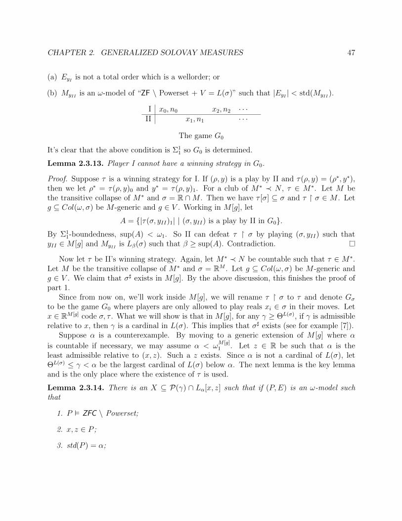
CHAPTER 2. GENERALIZED SOLOVAY MEASURES 47
(a) EyI is not a total order which is a wellorder; or
(b) MyII is an ω-model of “ZF \ Powerset + V = L(σ)” such that |EyI | < std(MyII ).
I x0, n0 x2, n2 · · ·II x1, n1 · · ·
The game G0
It’s clear that the above condition is Σ11 so G0 is determined.
Lemma 2.3.13. Player I cannot have a winning strategy in G0.
Proof. Suppose τ is a winning strategy for I. If (ρ, y) is a play by II and τ(ρ, y) = (ρ∗, y∗),then we let ρ∗ = τ(ρ, y)0 and y∗ = τ(ρ, y)1. For a club of M∗ ≺ N , τ ∈ M∗. Let M bethe transitive collapse of M∗ and σ = R ∩M . Then we have τ [σ] ⊆ σ and τ σ ∈ M . Letg ⊆ Col(ω, σ) be M -generic and g ∈ V . Working in M [g], let
A = |τ(σ, yII)1| | (σ, yII) is a play by II in G0.
By Σ11-boundedness, sup(A) < ω1. So II can defeat τ σ by playing (σ, yII) such that
yII ∈M [g] and MyII is Lβ(σ) such that β ≥ sup(A). Contradiction.
Now let τ be II’s winning strategy. Again, let M∗ ≺ N be countable such that τ ∈ M∗.Let M be the transitive collapse of M∗ and σ = RM . Let g ⊆ Col(ω, σ) be M -generic andg ∈ V . We claim that σ] exists in M [g]. By the above discussion, this finishes the proof ofpart 1.
Since from now on, we’ll work inside M [g], we will rename τ σ to τ and denote Gσ
to be the game G0 where players are only allowed to play reals xi ∈ σ in their moves. Letx ∈ RM [g] code σ, τ . What we will show is that in M [g], for any γ ≥ ΘL(σ), if γ is admissiblerelative to x, then γ is a cardinal in L(σ). This implies that σ] exists (see for example [7]).
Suppose α is a counterexample. By moving to a generic extension of M [g] where α
is countable if necessary, we may assume α < ωM [g]1 . Let z ∈ R be such that α is the
least admissible relative to (x, z). Such a z exists. Since α is not a cardinal of L(σ), letΘL(σ) ≤ γ < α be the largest cardinal of L(σ) below α. The next lemma is the key lemmaand is the only place where the existence of τ is used.
Lemma 2.3.14. There is an X ⊆ P(γ) ∩ Lα[x, z] such that if (P,E) is an ω-model suchthat
1. P ZFC \ Powerset;
2. x, z ∈ P ;
3. std(P ) = α;
CHAPTER 2. GENERALIZED SOLOVAY MEASURES 48
4. P τ is a winning strategy for II in Gσ and x enumerates σ, τ ;
then X = (P(γ) ∩ L(σ))P .
Proof. Let (P0, E0), (P1, E1) be two ω-models satisfying (1)-(4). We will occasionally con-fuse the set Pi with the structure (Pi, Ei). We further assume that RP0 ∩ RP1 = RLα[x,z]
and P(γ)P0 ∩ P(γ)P1 = P(γ)Lα[x,z]. Given any ω-model (P0, E0) satisfying (1)-(4), we canalways find an ω-model (P1, E1) satisfying (1)-(4) and is ”divergent” from (P0, E0) in theabove sense. We want to show (P (γ)∩L(σ))P0 = (P (γ)∩L(σ))P1 . Let A ∈ (P (γ)∩L(σ))P0 .We show that A ∈ (P (γ) ∩ L(σ))P1 . Of course, the converse is symmetrical.
Let a0 ∈ OrdP0 be such that a > α = std(P0), a is additively closed19, and (P0, E0) “A ∈ La0(σ).” Let a1 ∈ P1 be such that a1 > α and a1 is additively closed. The followingfact is key.
Claim 1: (b | bE0a0) ∼= (b | bE1a1) ∼= α + αQ.
Proof. We prove (b | bE0a0) ∼= α + αQ; the other equality is similar. We define anequivalence ∼ on a0 as follows. Let a, b ∈ OrdP0 be such that aE0a0 and bE0a, we say
a ∼ b⇔ ∃β < α(a = β + b ∨ b = β + a).
Clearly, ∼ is an equivalence relation on the set b ∈ OrdP0 | bE0a. We claim that for allbE0a0, [b]∼ has an E0-least element. To see this, first note that for any β < α, [β]∼ = [0]∼has an E0-least element, namely 0. Now suppose b /∈ std(P0). Note then that the set
b− a | aE0b
is finite in P0 and hence is actually finite since P0 is an ω-model and hence it is correct aboutfiniteness. This in turns implies the set
b− β | βE0b ∧ β < α
is non-empty, finite, and is bounded in α. But this implies [b]∼ has an E0-least element asclaimed.
Now let c, d /∈ std(P0) be such that cE0dE0a0 and c d. We want to show that there isan e such that cE0eE0d, c e, and e d. To this end, let d∗ = min([d]∼). By the claimabove, d∗ exists and cE0d
∗ and c d∗. But this means c+ β | β < α is not cofinal in d∗,so we can choose an e such that cE0eE0d
∗ as required.The above shows that [c]∼ | cE0a0 ∼= 1 +Q, which implies c | cE0a0 ∼= α + αQ.
Claim 1 implies that Col(ω, a0)P0 ∼= Col(ω, a1)P1 ∼= Col(ω, α + αQ). Next we build twogenerics G0, G1 as follows:
(a) Gi is Pi generic for Col(ω, ai) where i = 0, 1;
19This means for all bE0a0, b+ a0 = a0.
CHAPTER 2. GENERALIZED SOLOVAY MEASURES 49
(b) (i, j) | G0(i)E0G0(j) = (i, j) | G1(i)E1G1(j);
(c) P0 ∩ P0[G0] = P0, P1 ∩ P1[G1] = P1, P0 ∩ P1[G1] = P0 ∩ P1, and P1 ∩ P0[G0] = P0 ∩ P1;
(d) Pi[Gi] τ is a winning strategy for II in Gσ.
The requirement (b) can be ensured by a standard back-and-forth argument and the require-ment (c) can be ensured by choosing sufficiently generic G0 and G1. The requirement (d) isjust by Σ1
1-absoluteness.Now let h ∈ R be such that Eh = (i, j) | G0(i)E0G0(j).
Claim 2: A ∈ P1[G1].
Proof. First mote that h ∈ P0[G0] ∩ P1[G1] and hence τ(σ, h) ∈ P0[G0] ∩ P1[G1]. Wethen have P0[G0] “h gives a wellordering of length a0 and τ(σ, h) codes a model of V =L(σ) with standard part > a0.” This means P0[G0] “A is coded by τ(σ, h).” Since τ(σ, h)∈ P1[G1], A ∈ P1[G1].
Claim 2 implies A ∈ P1[G1] ∩ P0. c) implies that A ∈ P1. Hence we’re done.
Using Lemma 2.3.14, we get.
Lemma 2.3.15. Let Rγ ⊆ γ and Rγ ∈ Lγ+1(σ) be a coding of the canonical bijectione : γ × γ → γ. Let X be as in Lemma 2.3.14, then X ⊆ L(σ) and in fact,
(X, γ,Rγ,∈) ≺ (P (γ) ∩ L(σ), γ, Rγ,∈).
Proof. We prove X ⊆ L(σ), the proof of that
(X, γ,Rγ,∈) ≺ (P (γ) ∩ L(σ), γ, Rγ,∈)
is very similar. Let A ∈ X. By definition of X, A ∈ Lα[x, z]. Suppose A /∈ L(σ). This is afact in M [g] about A, x, z, α, σ; hence, there is an ω-model P in M [g] such that
• P ZFC \ Powerset;
• x, z, σ, z ∈ P and P τ is II’s winning strategy for Gσ and x enumerates σ, τ ;
• α = std(P );
• P A /∈ L(σ).
This contradicts the Lemma 2.3.14.
Let κ = (γ+)L(σ). Let X be as in Lemmata 2.3.14 and 2.3.15 and let Lη(σ) be the tran-sitive collapse of X.
Claim: η < α.
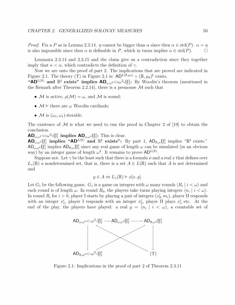
CHAPTER 2. GENERALIZED SOLOVAY MEASURES 50
Proof. Fix a P as in Lemma 2.3.14. η cannot be bigger than α since then α ∈ std(P ). α = ηis also impossible since then α is definable in P , which in turns implies α ∈ std(P ).
Lemmata 2.3.14 and 2.3.15 and the claim give us a contradiction since they togetherimply that κ < α, which contradicts the definition of γ.
Now we are onto the proof of part 2. The implications that are proved are indicated inFigure 2.1. The theory (T) in Figure 2.1 is: ADL(R,µ0) + (R, µ0)] exists.“ADL(R) and R] exists” implies ADω,ω2<-ω2-Π˜1
1: By Woodin’s theorem (mentioned inthe Remark after Theorem 2.2.14), there is a premouse M such that
• M is active, ρ(M) = ω, and M is sound;
• M there are ω Woodin cardinals;
• M is (ω1, ω1)-iterable.
The existence of M is what we need to run the proof in Chapter 2 of [19] to obtain theconclusion.ADω,ω2<-ω2-Π˜1
1 implies ADω,ω2Π˜11: This is clear.
ADω,ω2Π˜11 implies “ADL(R) and R] exists”: By part 1, ADR,ωΠ˜1
1 implies “R] exists.”ADω,ω2Π˜1
1 implies ADR,ωΠ˜11 since any real game of length ω can be simulated (in an obvious
way) by an integer game of length ω2. It remains to prove ADL(R).Suppose not. Let γ be the least such that there is a formula φ and a real x that defines over
Lγ(R) a nondetermined set, that is, there is a set A ∈ L(R) such that A is not determinedand
y ∈ A⇔ Lγ(R) φ[x, y].
Let G1 be the following game. G1 is a game on integers with ω many rounds 〈Ri | i < ω〉 andeach round is of length ω. In round R0, the players take turns playing integers 〈ni | i < ω〉.In round Ri for i > 0, player I starts by playing a pair of integers (xi0,mi), player II respondswith an integer xi1, player I responds with an integer xi2, player II plays xi3 etc. At theend of the play, the players have played: a real y = 〈ni | i < ω〉, a countable set of
ADω,ω3<-ω2-Π˜11
ADR,ω2<-ω2-Π˜11
ADω,ω3Π˜11 ADR,ω2Π˜1
1
(T)
Figure 2.1: Implications in the proof of part 2 of Theorem 2.3.11
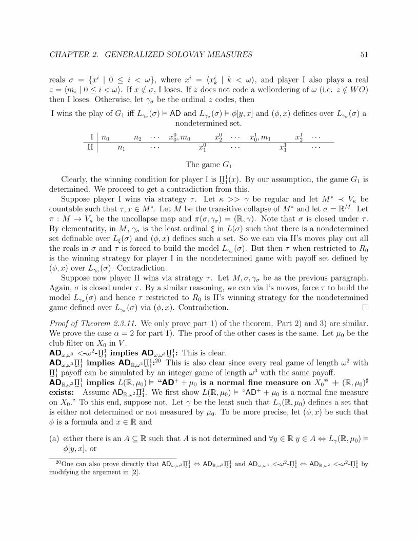
CHAPTER 2. GENERALIZED SOLOVAY MEASURES 51
reals σ = xi | 0 ≤ i < ω, where xi = 〈xik | k < ω〉, and player I also plays a realz = 〈mi | 0 ≤ i < ω〉. If x /∈ σ, I loses. If z does not code a wellordering of ω (i.e. z /∈ WO)then I loses. Otherwise, let γσ be the ordinal z codes, then
I wins the play of G1 iff Lγσ(σ) AD and Lγσ(σ) φ[y, x] and (φ, x) defines over Lγσ(σ) anondetermined set.
I n0 n2 · · · x00,m0 x0
2 · · · x10,m1 x1
2 · · ·II n1 · · · x0
1 · · · x11 · · ·
The game G1
Clearly, the winning condition for player I is Π˜11(x). By our assumption, the game G1 is
determined. We proceed to get a contradiction from this.Suppose player I wins via strategy τ . Let κ >> γ be regular and let M∗ ≺ Vκ be
countable such that τ, x ∈M∗. Let M be the transitive collapse of M∗ and let σ = RM . Letπ : M → Vκ be the uncollapse map and π(σ, γσ) = (R, γ). Note that σ is closed under τ .By elementarity, in M , γσ is the least ordinal ξ in L(σ) such that there is a nondeterminedset definable over Lξ(σ) and (φ, x) defines such a set. So we can via II’s moves play out allthe reals in σ and τ is forced to build the model Lγσ(σ). But then τ when restricted to R0
is the winning strategy for player I in the nondetermined game with payoff set defined by(φ, x) over Lγσ(σ). Contradiction.
Suppose now player II wins via strategy τ . Let M,σ, γσ be as the previous paragraph.Again, σ is closed under τ . By a similar reasoning, we can via I’s moves, force τ to build themodel Lγσ(σ) and hence τ restricted to R0 is II’s winning strategy for the nondeterminedgame defined over Lγσ(σ) via (φ, x). Contradiction.
Proof of Theorem 2.3.11. We only prove part 1) of the theorem. Part 2) and 3) are similar.We prove the case α = 2 for part 1). The proof of the other cases is the same. Let µ0 be theclub filter on X0 in V .ADω,ω3 <-ω2-Π˜1
1 implies ADω,ω3Π˜11: This is clear.
ADω,ω3Π˜11 implies ADR,ω2Π˜1
1:20 This is also clear since every real game of length ω2 with
Π˜11 payoff can be simulated by an integer game of length ω3 with the same payoff.
ADR,ω2Π˜11 implies L(R, µ0) “AD+ + µ0 is a normal fine measure on X0” + (R, µ0)]
exists: Assume ADR,ω2Π˜11. We first show L(R, µ0) “AD+ + µ0 is a normal fine measure
on X0.” To this end, suppose not. Let γ be the least such that Lγ(R, µ0) defines a set thatis either not determined or not measured by µ0. To be more precise, let (φ, x) be such thatφ is a formula and x ∈ R and
(a) either there is an A ⊆ R such that A is not determined and ∀y ∈ R y ∈ A⇔ Lγ(R, µ0) φ[y, x], or
20One can also prove directly that ADω,ω3Π˜11 ⇔ ADR,ω2Π˜1
1 and ADω,ω3 <-ω2-Π˜11 ⇔ ADR,ω2 <-ω2-Π˜1
1 bymodifying the argument in [2].
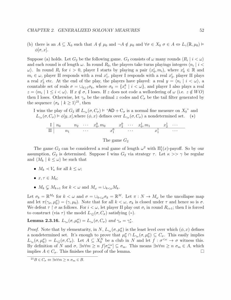
CHAPTER 2. GENERALIZED SOLOVAY MEASURES 52
(b) there is an A ⊆ X0 such that A /∈ µ0 and ¬A /∈ µ0 and ∀σ ∈ X0 σ ∈ A ⇔ Lγ(R, µ0) φ[σ, x].
Suppose (a) holds. Let G2 be the following game. G2 consists of ω many rounds 〈Ri | i < ω〉and each round is of length ω. In round R0, the players take turns playings integers 〈ni | i <ω〉. In round Ri for i > 0, player I starts by playing a pair (xi0,mi), where xi0 ∈ R andmi ∈ ω, player II responds with a real xi1, player I responds with a real xi2, player II playsa real xi3 etc. At the end of the play, the players have played: a real y = 〈ni | i < ω〉, acountable set of reals σ = ∪k≥1σk, where σk = xki | i < ω, and player I also plays a realz = 〈mi | 1 ≤ i < ω〉. If x /∈ σ, I loses. If z does not code a wellordering of ω (i.e. z /∈ WO)then I loses. Otherwise, let γσ be the ordinal z codes and Cσ be the tail filter generated bythe sequence 〈σk | k ≥ 1〉21, then
I wins the play of G2 iff Lγσ(σ,Cσ) “AD + Cσ is a normal fine measure on X0” andLγσ(σ,Cσ) φ[y, x],where (φ, x) defines over Lγσ(σ,Cσ) a nondetermined set. (*)
I n0 n2 · · · x00,m0 x0
2 · · · x10,m1 x1
2 · · ·II n1 · · · x0
1 · · · x11 · · ·
The game G2
The game G2 can be considered a real game of length ω2 with Π11(x)-payoff. So by our
assumption, G2 is determined. Suppose I wins G2 via strategy τ . Let κ >> γ be regularand 〈Mk | k ≤ ω〉 be such that
• Mk ≺ Vκ for all k ≤ ω;
• x, τ ∈M0;
• Mk (Mk+1 for k < ω and Mω = ∪k<ωMk.
Let σk = RMk for k < ω and σ = ∪k<ωσk = RM . Let π : N → Mω be the uncollapse mapand let π(γσ, µ
σ0 ) = (γ, µ0). Note that for all k < ω, σk is closed under τ and hence so is σ.
We defeat τ σ as follows. For i < ω, let player II play out σi in round Ri+1; then I is forcedto construct (via τ) the model Lγ∗σ(σ,Cσ) satisfying (*).
Lemma 2.3.16. Lγσ(σ, µσ0 ) = Lγσ(σ,Cσ) and γσ = γ∗σ.
Proof. Note that by elementarity, in N , Lγσ(σ, µσ0 ) is the least level over which (φ, x) definesa nondetermined set. It’s enough to prove that µσ0 ∩ Lγσ(σ, µσ0 ) ⊆ Cσ. This easily impliesLγσ(σ, µσ0 ) = Lγ∗σ(σ,Cσ). Let A ⊆ XN
0 be a club in N and let f : σ<ω → σ witness this.By definition of N and σ, ∃n∀m ≥ n f [σ<ωm ] ⊆ σm. This means ∃n∀m ≥ n σm ∈ A, whichimplies A ∈ Cσ. This finishes the proof of the lemma.
21B ∈ Cσ ⇔ ∃n∀m ≥ n σm ∈ B.
CHAPTER 2. GENERALIZED SOLOVAY MEASURES 53
By the lemma, in N , τ σ when restricted to R0 of G2 is I’s winning strategy for thenondetermined game defined by (φ, x) over Lγσ(σ, µσ0 ). Contradiction. A similar (and a biteasier) reasoning gives a contradiction from the assumption that II has a winning strategyin G2.
Now suppose (b) holds. Then (φ, x) defines over Lγ(R, µ0) a set A such that A /∈ µ0 and¬A /∈ µ0. Let G3 be the following game. G3 has ω rounds Ri | i < ω and each round isof length ω. For i < ω, player I starts round Ri by playing a pair (xi0, ni), where xi0 ∈ Rand ni ∈ ω, II responds with a real xi1, I then responds with a ral xi2, II plays a real xi3 inresponse etc. Let σi = xik | k < ω. Additionally, if i > 0, we require that the real xi0 mustcode σi−1
22 (otherwise, I loses). At the end of the play, let σ = ∪iσi, y = 〈ni | i < ω〉, andlet Cσ be the tail filter defined by the sequence 〈σi | i < ω〉. If y /∈ WO, I loses. Otherwise,letting γσ be the ordinal coded by y, then
I wins the play of G3 ⇔ x ∈ σ0 and Lγσ(σ,Cσ) “AD +Cσ is a normal fine measure on X0”and (φ, x) defines over Lγσ(σ,Cσ) a set not measured by Cσ and σ0 ∈ Cσ. (**)
I x00, n0 x0
2 · · · x10 (codes σ0), n1 x1
2 · · ·II x0
1 · · · x11 · · ·
The game G3
The winning condition for player I in G3 is Π11(x) so G3 is determined. First let τ be I’s
winning strategy. Let κ >> γ be regular and 〈Mk | k ≤ ω〉 be such that
• Mk ≺ Vκ for all k ≤ ω;
• x, τ ∈M0;
• Mk (Mk+1 for k < ω and Mω = ∪k<ωMk.
Let σk = RMk for k < ω and σ = ∪k<ωσk = RM . Let π : N → Mω be the uncollapse mapand let π(γσ, µ
σ0 ) = (γ, µ0). Note that for all k < ω, σk is closed under τ and hence so is
σ. We defeat τ σ as follows. We consider the following sequence 〈Pn | n < ω〉, whereeach Pn is a complete play of G3 according τ . We describe how II plays in Pn. In roundRi, II plays out σi+n (since σi+n is closed under τ , at the end of round Ri, the players playout the countable set of reals σi+n). At the end of the play Pn, the players play out thesequence Sn = 〈σi+n | i < ω〉 (note that ∪Sn = σ) and τ constructs a model Lγn(σ,Cn)satisfying (**), where Cn is the tail filter given by Sn. Note that Cn = Cm for all n,m. LetC be Cn for some (any) n. Hence by the fact that Lγn(σ,Cn) satisfies (**), for all n,m,Lγn(σ,Cn) = Lγm(σ,Cm). Let ξ = γn for some (any) n. Let A be the set not measured by Cdefined by (φ, x) over Lξ(σ,C). Recall that for each n, the countable set of reals played outin R0 of Pn is σn, we have by the fact that τ is I’s winning strategy that σn ∈ A. So A ∈ C
22This just means that xi0 can compute an enumeration in order type ω of σi−1
CHAPTER 2. GENERALIZED SOLOVAY MEASURES 54
after all. Contradiction.Assume now II has a winning strategy in G3. The same reasoning as above gives us a
contradiction. The only difference is we get that for all n, σn /∈ A so ¬A ∈ C.Now it remains to prove (R, µ0)] exists. The proof is a combination of techniques used
in the proof that ADR,ω2Π˜11 ⇒ L(R, µ0) “AD+ + µ0 is a normal fine measure on X0” and
ADR,ωΠ˜11 ⇒ R] exists. We sketch only the proof here.
Recall that at this point, we have proved L(R, µ0) AD+ +µ0 is a normal fine measure onX0. We describe a real game G of length ω2 with Π1
1 payoff. A typical play of G is as follows.At round Ri, player I starts the round by playing (xi0, ni) where xi0 ∈ R, ni ∈ ω, player IIresponds with (xi1,mi) where xi1 ∈ R, mi ∈ ω, player I responds with xi2, player II plays xi3in response. In general, for k ≤ 1, player I plays a real xi2k while player II plays a real xi2k+1.At the end of the play, the players play a sequence 〈σi | i < ω〉, where σi = xij | j < ω,player I plays a real x = 〈ni | i < ω〉, and player II plays a real y = 〈mi | i < ω〉. Let C bethe tail filter generated by the sequence 〈σi | i < ω〉 and σ = ∪iσi.
Using the notation introduced in the proof of ADR,ωΠ˜11 ⇒ R], Player II wins the play if
(a) Ex is not a total order which is a wellorder; or
(b) My is an ω-model of “ZF \ Powerset + V = L(σ,C) + AD+ + C is a normal fine measureon X0” such that |Ex| < std(My).
Again, G is determined and player I cannot have a winning strategy in G. Hence II hasa winning strategy τ . Let κ be a large, regular cardinal in V , and M∗ ≺ Vκ be countablesuch that M∗ is the union of an increasing sequence 〈M∗
n | n < ω〉 of countable elementarysubstructures of Vκ and τ ∈ M∗
0 . Let M be the transitive collapse of M∗ and π is theuncollapse map. Let π(σ, µσ0 ) = (R, µ0). Let g ⊆ Col(ω, σ) be M -generic and g ∈ V .We prove that σ] exists in M [g] by proving in M [g], there is a real x such that for everyγ ≥ ΘL(σ,µσ0 ), if γ is admissible relative to x then γ is a cardinal in L(σ, µσ0 ). The rest of theproof is similar to that of the corresponding part in the proof of ADR,ωΠ˜1
1 ⇒ R]. We leavethe details to the reader.L(R, µ0) “AD+ + µ0 is a normal fine measure on X0” + (R, µ0)] exists impliesADω,ω3 <-ω2-Π˜1
1: Theorem 4.2.5 implies there is a premouse M such that
• M is active, ρ(M) = ω, and M is sound;
• M there are ω2 Woodin cardinals;
• M is (ω1, ω1)-iterable.
The existence of M is what we need to run the proof in Chapter 2 of [19] to obtain theconclusion.ADω,ω3 <-ω2-Π˜1
1 implies ADR,ω2 <-ω2-Π˜11: This is again clear since every real game of
length ω2 with <-ω2-Π˜11 payoff can be simulated by an integer game of length ω3 with the
CHAPTER 2. GENERALIZED SOLOVAY MEASURES 55
same payoff.ADR,ω2 <-ω2-Π˜1
1 implies ADR,ω2Π˜11: This is also clear.
The above implications cover all the equivalences that need to be proved. Hence we’redone.
56
Chapter 3
HOD Analysis
3.1 When V = L(P(R))
3.1.1 The Successor Case
3.1.1.1 Preliminaries
Let (P ,Σ) be a hod pair such that Σ has branch condensation. We let KΣ,−(R) be theunion of all N such that N is a Σ-premouse over R (in the sense of [27])1, ρω(R) = R, andwhenever M is countable transitive such that P ∈M and M elementarily embeds into N ,thenM has a unique ω1 + 1-iteration strategy Λ such that whenever Q is a Λ-iterate ofM,then Q is also a Σ-premouse. We say M is Σ-iterable. Finally, let KΣ(R) = L(KΣ,−(R)).
Let (P ,Σ) be as above. We briefly describe a notion of Prikry forcing that will beuseful in our HOD computation. The forcing P described here is defined in KΣ(R) and isa modification of the forcing defined in Section 6.6 of [41]. All facts about this forcing areproved similarly as those in Section 6.6 of [41] so we omit all proofs.
First, let T be the tree of a Σ21(Σ) scale on a universal Σ2
1 set U . Write Px for theΣ-premouse coded by the real x. Let a be countable transitive, x ∈ R such that a is codedby a real recursive in x. A normal iteration tree U on a 0-suitable Σ-premouse Q (seeDefinition 3.1.20, where (Q,Σ) is defined to be 0-suitable) is short if for all limit ξ ≤ lh(U),LpΣ(M(U|ξ)) δ(U|ξ) is not Woodin. Otherwise, we say that U is maximal. We say that a0-suitable Pz is short-tree iterable by Λ if for any short tree T on Pz, b = Λ(T ) is such thatMT
b is 0-suitable, and b has a Q-structure Q such that Q EMTb . Put
Fxa = Pz | z ≤T x,Pz is a short-tree iterable 0-suitable Σ-premouse over a
For each a, for x in the cone in the previous claim, working in L[T, x], we can simultaneouslycompare all Pz ∈ Fxa (using their short-tree iteration strategy) while doing the genericity
1Here we assume Σ is sufficiently iterable that the definition of Σ-premouse over R makes sense; see [27]for more details.
CHAPTER 3. HOD ANALYSIS 57
iterations to make all y such that y ≤T x generic over the common part of the final modelQx,−a . This process (hence Qx,−a ) depends only on the Turing degree of x. Put
Qxa = LpΣω(Qx,−a ), and δxa = o(Qx,−a ).
By the above discussion, Qxa, δxa depend only on the Turing degree of x. Here are someproperties obtained from the above process.
1. Fxa 6= ∅ for x of sufficiently large degree;
2. Qx,−a is full (no levels of Qxa project strictly below δxa);
3. Qxa δxa is Woodin;
4. P(a) ∩Qxa = P(a) ∩ODT (a ∪ a) and P(δxa) ∩Qxa = P(δxa) ∩ODT (Qx,−a ∪ Qx,−
a );
5. δxa = ωL[T,x]1 .
Now for an increasing sequence ~d = 〈d0, ..., dn〉 of Turing degrees, and a countable transitive,set
Q0(a) = Qd0a and Qi+1(a) = Qdi+1
Qi(a) for i < n
We assume from here on that the degrees di+1’s are such that Qdi+1
Qi(a) are defined. For ~d as
above, write Q~di (a) = Qi(a) even though Qi(a) only depends on ~d|(i+ 1). Let µ be the cone
measure on the Turing degrees. We can then define our Prikry forcing P (over L(T,R)) as
follows. A condition (p, S) ∈ P just in case p = 〈Q~d0(a), ...,Q~d
n(a)〉 for some ~d, S ∈ L(T,R) is a“measure-one tree” consisting of stems q which either are initial segments or end-extensionsof p and such that (∀q = 〈Q~e0(a), ...,Q~ek(a)〉 ∈ S)(∀∗µd) let ~f = 〈~e(0), ..., ~e(k), d〉, we have
〈Q~f0(a), ...,Q~f
(k+1)(a)〉 ∈ S. The ordering on P is defined as follows.
(p, S) 4 (q,W ) iff p end-extends q, S ⊆ W , and ∀n ∈ dom(p)\ dom(q) (p|(n+ 1) ∈ W ).
P has the Prikry property in KΣ(R). Let G be a P-generic over KΣ(R), 〈Qi | i < ω〉 =
∪p | ∃ ~X(p, ~X) ∈ G and Q∞ =⋃iQi. Let δi be the largest Woodin cardinal of Qi. Then
P (δi) ∩ L[T, 〈Qi | i < ω〉] ⊆ Qi,
and
L[T,Q∞] = L[T, 〈Qi | i < ω〉] δi is Woodin.
Definition 3.1.1 (Derived models). Suppose M ZFC and λ ∈ M is a limit of Woodincardinals in M . Let G ⊆ Col(ω,< λ) be generic over M . Let R∗G (or just R∗) be thesymmetric reals of M [G] and Hom∗G (or just Hom∗) be the set of A ⊆ R∗ in M(R∗) suchthat there is a tree T such that A = p[T ] ∩ R∗ and there is some α < λ such that
CHAPTER 3. HOD ANALYSIS 58
M [G α] “T has a <-λ-complement”.
By the old derived model of M at λ, denoted by D(M,λ), we mean the model L(R∗, Hom∗).By the new derived model of M at λ, denoted by D+(M,λ), we mean the model L(Γ,R∗),where Γ is the closure under Wadge reducibility of the set of A ∈ M(R∗) ∩ P(R∗) such thatL(A,R∗) AD+.
Theorem 3.1.2 (Woodin). Let M be a model of ZFC and λ ∈ M be a limit of Woodincardinals of M . Then D(M,λ) AD+, D+(M,λ) AD+. Furthermore, Hom∗ is thepointclass of Suslin co-Suslin sets of D+(M,λ).
Using the proof of Theorem 3.1 from [36] and the definition of KΣ(R) from [27], we get thatin KΣ(R)[G], there is a Σ-premouse Q+
∞ extending Q∞ such that KΣ(R) can be realizedas a (new) derived model of Q+
∞ at ωV1 , which is the limit of Woodin cardinals of Q+∞.
Roughly speaking, the Σ-premouse Q+∞ is the union of Σ-premice R over Q∞, where R is
an S-translation of some MKΣ(R) (see [23] for more on S-translations).
3.1.1.2 When α = 0
We recall some basic notions from descriptive inner model theory. All the notions andnotations used in this section are standard. See [26] and [38] for full details. Here, we’ll tryto stay as close notationally as possible to those used in [26] and [38]. The reader who arefamiliar with basic descriptive inner model theory can skip ahead to the actual computationand come back to this when necessary.
Definition 3.1.3 (k-suitable premouse). Let 0 ≤ k < ω and Γ be an inductive-like pointclass.A premouse N is k-suitable with respect to Γ iff there is a strictly increasing sequence 〈δi | i ≤k〉 such that
1. for all δ, N “δ is Woodin” iff δ = δi for some i < 1 + k;
2. ORN = sup((δ+nk )N |n < ω);
3. LpΓ(N|ξ) = N|(ξ+)+ for all cutpoints ξ of N where LpΓ(N|ξ) = ∪M | N|ξ M∧ρ(M) = ξ ∧M has iteration strategy in Γ;
4. if ξ ∈ OR ∩N and ξ 6= δi for all i, then LpΓ(N|ξ) ”ξ is not Woodin.”
Definition 3.1.4. Let N be as above and A ⊆ R. Then τNA,ν is the unique standard termσ ∈ N such that σg = A∩N [g] for all g generic over N for Col(ω, ν), if such a term exists.We say that N term captures A iff τNA,ν exists for all cardinals ν of N .
If N ,Γ are as in Definition 2.1 and A ∈ Γ, then [26] shows that N term captures A.Later on, if the context is clear, we’ll simply say capture instead of term capture or Suslincapture. For a complete definition of “N is A-iterable”, see [38]. Roughly speaking, N isA-iterable if N term captures A and
CHAPTER 3. HOD ANALYSIS 59
1. for any maximal tree T (or stack ~T ) on N , there is a cofinal branch b such that thebranch embedding iTb =def i moves the term relation for A correctly i.e., for any κ
cardinal in N , i(τNA,κ) = τMTbA,i(κ);
2. if T on N is short, then there is a branch b such that Q(b, T )2 exists and Q(b, T ) LpΓ(M(T ))3; we say that T ab is Γ-guided.
This obviously generalizes to define ~A-iterability for any finite sequence ~A.
Definition 3.1.5. Let N be k-suitable with respect to Σ21 and k < ω. Let ~A = 〈Ai | i ≤ n〉
be a sequence of OD sets of reals and ν = (δ+ωk )N . Then
1. γN~A = sup(ξ|ξ is definable over (N|ν, τNA0,δk, ..., τNAn,δk) ∩ δ0);
2. HN~A = HullN (γN~A ∪ τNA0,δk
, ..., τNAn,δk), where we take the full elementary hull withoutcollapsing.
From now on, we will write τNA without further clarifying that this stands for τNA,δ whereδ is the largest Woodin cardinal of N . We’ll also write τNA,l for τN
A,δNlfor l ≤ k. Also, we’ll
occasionally say k-suitable without specifying the pointclass Γ.
Definition 3.1.6. Let N be k-suitable with respect to some pointclass Γ and A ∈ Γ. N isstrongly A-iterable if N is A-iterable and for any suitable M such that if i, j : N →M aretwo A-iteration maps then i HNA = j HMA .
Definition 3.1.7. Let Γ be an inductive-like pointclass and N be k-suitable with respect toΓ for some k. Let A be a countable collection of sets of reals in Γ ∪ Γ. We say A guides astrategy for N below δN0 if whenever T is a countable, normal iteration tree on N based onδN0 of limit length, then
1. if T is short, then there is a unique cofinal branch b such that Q(b, T ) exists andQ(b, T ) LpΓ(M(T ))4, and
2. if T is maximal, then there is a unique nondropping branch b such that iTb (τNA,µ) =
τMTbA,ib(µ) for all A ∈ A and cardinals µ ≥ δNk of N and δ(T ) = supγM
Tb
A,0 | A ∈ A where
δ = iTb (δ0).
2Q(b, T ) is called the Q-structure and is defined to be the least initial segment of MTb that defines thefailure of Woodinness of δ(T ).
3This implicitly assumes that Q(b, T ) has no extenders overlapping δ(T ). We’re only interested in treesT arising from comparisons between suitable mice and for such trees, Q structures have no extenders over-lapping δ(T ).
4Again we disregard the case where Q-structures have overlapping extenders.
CHAPTER 3. HOD ANALYSIS 60
We can also define an A-guided strategy that acts on finite stacks of normal trees in a similarfashion.
The most important instance of the above definition used in this paper is when A isa self-justifying-system that seals a Σ1 gap. A strategy guided by such an A has manydesirable properties.
We state a theorem of Steel’s which essentially says that Mouse Capturing implies MouseCapturing for mice over R.
Theorem 3.1.8 (Steel, see [35]). Assume AD+ + V = L(P(R)) + Θ = θ0 + MC5. Thenevery set of reals is in a (countably iterable) mouse over R projecting to R. In other words,V = K(R), where
K(R) = L(∪M | M is R-sound, ρω(M) = R, and M is countably iterable).
Next, we prove the following theorem of Woodin’s which roughly states that HOD iscoded into a subset of Θ.
Theorem 3.1.9 (Woodin). Assume AD+ + V = L(P(R)). Then HOD = L[P ] for someP ⊆ Θ in HOD.
Proof. First, let
P = (~α,~a) | ~α = 〈α0, α1, ..., αn〉 ∈ Θ<ω,~a = 〈a0, a1, ..., an〉,∀i ≤ n(ai ⊆ αi).
P is a poset with the (obvious) order by extension. If g is a P-generic over V then g inducesan enumeration of order type ω of (Θ,∪γ<ΘP(γ)). Now let
Q∗ = (~α,A) | ~α = 〈α0, α1, ..., αn〉 ∈ Θ<ω, A ⊆ P(α0)× P(α1)× ...× P(αn), A ∈ OD.
The ordering on Q∗ is defined as follows:
(~α,A) ≤ (~β,B)⇔ ∀i < dom(~α)~α(i) = ~β(i), B|(P(~α(0))× ...× P(~α(dom(α)− 1)))6 ⊆ A.
There is a poset Q ∈ HOD ∩ P(Θ) that is isomorphic to Q∗ via an OD map π. For ourconvenience, whenever p ∈ Q, we will write p∗ for π(p). Furthermore, we can define π sothat elements of Q have the form (~α,A) whenever p∗ = (~α,A∗). In other words, we canthink of π as a bijection of Θ and the set of OD subsets of P(α0)×P(α1)× ...×P(αn) forα0, α1, ..., αn < Θ. For notational simplicity, if p∗ = (~α,A∗), we write o(p∗) for ~α and s(p∗)for A∗.
Claim 1. Let g be P-generic over V . Then g induces a Q-generic Gg over HOD. Infact, for any condition q ∈ Q, we can find a P-generic g over V such that q ∈ Gg and Gg isa Q-generic over HOD.
5MC stands for Mouse Capturing, which states that if x, y ∈ R and x ∈ OD(y) then x is in a sound mouseover y projecting to y.
CHAPTER 3. HOD ANALYSIS 61
Proof. As mentioned above, g induces a generic enumeration f of (Θ,∪γ<ΘP(γ)) of ordertype ω. Furthermore, for each n < ω, f(n)0 < Θ and f(n)1 ⊆ f(n)0. Let
G = ∪n<ω(〈f(0)0, ..., f(n)0〉, A) ∈ Q | 〈f(0)1, ..., f(n)1〉 ∈ A∗.
We claim that G is Q-generic over HOD. To see this, let D ⊆ Q, D ∈ HOD be a denseset. Let p = f |(n + 1) for some n. It’s enough to find a q = (〈α0, ..., αm〉, 〈a0, ..., am〉) ∈ Pextending p such that Dq ∩D 6= ∅ where
Dq = (〈α0, ..., αm〉, A) | 〈a0, ..., am〉 ∈ A∗.
If no such q exists, let r = (〈f(0)0, ..., f(n)0〉, B), where
b ∈ B∗ ⇔ ∀t ∈ D∀c(bac /∈ s(t)).
Then r is a condition in Q with no extension in D. Contradiction.
For each α < Θ, n < ω, and 〈α0, ..., αn〉, let Aα,〈α0,...,αn〉 = (〈α0, ..., αn〉, A) such that∀a ∈ A∗(α ∈ a(n)). We can then define a canonical term in HOD for a generic enumerationof ∪γ<ΘP(γ). For each n < ω, let σn = (p, α) | p ∈ Q, p ≤ Aα,〈α0,...,αn〉 for some 〈α0, ..., αn〉 ∈Θn+1; let τ = (A, σn) | n < ω,A ∈ Q. Then it’s easy to see that whenever G is P-genericover HOD induced by a P-generic over V , τG enumerates ∪γ<ΘP(γ) in order type ω. Thismeans we can recover P(R)V in the model L[Q, τ ][G] by AD+ (here we only use the fact thatevery set of reals has an ∞-Borel code which is a bounded subset of Θ).
To sum up, we have L[Q, τ ] ⊆ HOD ⊆ L[Q, τ ][G] for some Q-generic G over HOD. Bya standard argument, this implies that L[Q, τ ] = HOD.
Now let F = (M, ~A) | ~A is a finite sequence of OD sets of reals and M is k-suitable for
some k and is strongly ~A-iterable. We say (M, ~A) ≤F (N , ~B) if ~A ⊆ ~B and M iterates
to a suitable initial segment of N , say N−, via its iteration strategy that respects ~A. Wethen let π(M, ~A),(N , ~B) : HM~A → HN
−
~Bbe the unique map. That is, given any two different
iteration maps i0, i1 :M→N− according toM’s iteration strategy, by strong ~A-iterability,i0 HM~A = i1 HM~A , so the map π(M, ~A),(N , ~B) is well-defined. The following theorem isbasically due to Woodin. We just sketch the proof and give more details in the proof ofProposition 3.1.12.
Theorem 3.1.10. Assume V = L(P(R)) +AD+ +MC+ Θ = θ0. Given any OD set of realsA and any n ∈ ω, there is an n-suitable M that is strongly A-iterable. The same conclusionholds for any finite sequence ~A of OD sets of reals.
Proof. We’ll prove the theorem for n = 1. The other cases are similar. So suppose not. ByTheorem 3.1.8, V = K(R). Then V φ where φ = (∃α) (K(R)|α “ZF− + Θ exists +(∃A) (A is OD and there is no 1-suitable strongly A-iterable mouse))”.
CHAPTER 3. HOD ANALYSIS 62
Let γ < δ˜21 be least such that K(R)|γ φ. Such a γ exists by Σ1-reflection, i.e. Theorem
1.1.5. Then it is easy to see that γ ends a proper weak gap, say [γ, γ] for some γ < γ. Fixthe least such A as above. By [39] and the minimality of γ, we get a self-justifying-system(sjs) 〈Ai | i < ω〉 of ODK(R)|γ sets of reals in K(R)|γ that seals the gap7. We may and
do assume A = A0. Let Γ = ΣK(R)|γ1 and Ω a good pointclass beyond K(R)|(γ + 1), i.e.
P(R)K(R)|(γ+1) ( ∆˜Ω. Ω exists because γ < δ˜21. Let N∗ be a coarse Ω-Woodin, fully iterable
mouse. Such an N∗ exists by [35] or by Theorem 1.1.4. In fact by Theorem 1.1.4, one canchoose N∗ that Suslin captures Ω and the sequence 〈Ai | i < ω〉. Also by [35], there areclub-in-ORN∗ many Γ-Woodin cardinals in N∗. It can be shown that the L[E]-constructiondone inside N∗ reaches a P such that P is 1-suitable with respect to Γ (hence has canonicalterms for the Ai’s) and P “δ0 and δ1 are Woodin cardinals” where δ0 and δ1 are the firsttwo Γ-Woodin cardinals in N∗. Let Σ be the strategy for P induced by that of N∗. By liftingup to the background strategy and using term condensation for the self-justifying-system,we get that Σ is guided by 〈Ai | i < ω〉, hence (P ,Σ) is strongly A-iterable. But thenK(R)|γ ”P is strongly A-iterable.” This is a contradiction.
The theorem implies F 6= ∅. Moreover, we have that F is a directed system becausegiven any (M, ~A), (N , ~B) ∈ F , we can do a simultaneous comparison of (M, ~A), (N , ~B),
and some (P , ~A ⊕ ~B) ∈ F using their iteration strategies to obtain some (Q, ~A ⊕ ~B) ∈ Fsuch that (M, ~A), (N , ~B) ≤F (Q, ~A ⊕ ~B). We summarize facts about M∞ proved in [26]and [41]. These results are due to Woodin.
Lemma 3.1.11. 1. M∞ is wellfounded.
2. M∞ has ω Woodin cardinals (δM∞0 , δM∞1 ...) cofinal in its ordinals.
3. θ0 = δM∞0 and HOD|θ0 =M∞|δM∞0 .
We’ll extend this computation to the full HOD. Now we define a strategy Σ∞ for M∞.For each A ∈ OD ∩ P(R), let τM∞A,k = common value of π(P,A),∞(τPA,k) where π(P,A),∞ is
the direct limit map and τPA,k is the standard term of P that captures A at δPk . Σ∞ will
be defined (in V ) for (finite stacks of) trees on M∞|δM∞0 in M∞. For k ≥ n, M∞ “Col(ω, δM∞n )×Col(ω, δM∞k ) (τM∞A,n )g = (τM∞A,k )h∩M∞[g]” where g is Col(ω, δM∞n ) generic
and h is Col(ω, δM∞k ) generic. This is just saying that the terms cohere with one another.Let G be Col(ω,< λM∞) generic over M∞ where λM∞ is the sup of Woodin cardinals
in M∞. Then R∗G is the symmetric reals and A∗G := ∪k(τM∞A,k )G|δM∞k.
Proposition 3.1.12. For all A ⊆ R, A is OD, L(A∗G,R∗G) AD+.
7This means that for all i, ¬Ai and a scale for Ai are in 〈Ai | i < ω〉. Furthermore, the Ai’s are cofinalin the Wadge hierarchy of K(R)|γ.
CHAPTER 3. HOD ANALYSIS 63
Proof. Suppose not. Using Σ1-reflection, there is an N , which is a level of K(R) below δ˜21
satisfying the statement (T) ≡ “AD+ + ZF− + DC + MC + ∃A(A is OD and L(A∗G,R∗G) 2AD+))”. We may assume N is the first such level. Let
U = (x,M) :M is a sound x-mouse, ρω(M) = x, and has an iteration strategy in N.
Since MC holds in N , U is a universal (Σ21)N -set. Let A ∈ N be an OD set of reals witnessing
φ. We assume that A has the minimal Wadge rank among the sets witnessing φ. Using theresults of [46], we can get a ~B = 〈Bi : i < ω〉 which is a self-justifying-system (sjs) such thatB0 = U and each Bi ∈ N . Furthermore, we may assume that each Bi is OD in N .
Because MC holds and Γ∗ =def P(R)N ∆˜ 21, there is a real x such that there is a sound
mouse M over x such that ρ(M) = x and M doesn’t have an iteration strategy in N . Fixthen such an (x,M) and let Σ be the strategy of M. Let Γ be a good pointclass such that
Code(Σ), ~B, U, U c ∈ ∆˜Γ. Let F be as in Theorem 1.1.4 and let z be such that (N ∗z , δz,Σz)
Suslin captures Code(Σ), ~B, U, U c.
We let Φ = (Σ21)N . We have that Φ is a good pointclass. Because ~B is Suslin captured
by N ∗z , we have (δ+z )N
∗z -complementing trees T, S ∈ N ∗z which capture ~B. Let κ be the least
cardinal of N ∗z which, in N ∗z is < δz-strong.
Claim 1. N ∗z “κ is a limit of points η such that LpΓ∗(N ∗z |η) “η is Woodin”.
Proof. The proof is an easy reflection argument. Let λ = δ+z and let π : M → N ∗z |λ be an
elementary substructure such that
1. T, S ∈ ran(π),
2. if cp(π) = η then VN ∗zη ⊆M , π(η) = δz and η > κ.
By elementarity, we have that M “η is Woodin”. Letting π−1(〈T, S〉) = 〈T, S〉, we havethat (T, S) Suslin captures the universal Φ set over M at (η+)M . This implies that M isΦ-full and in particular, LpΓ∗(N ∗z |η) ∈ M . Therefore, LpΓ∗(N ∗z |η) “η is Woodin”. Theclaim then follows by a standard argument.
Let now 〈ηi : i < ω〉 be the first ω points < κ such that for every i < ω, LpΓ∗(N ∗z |ηi) “ηiis Woodin”. Let now 〈Ni : i < ω〉 be a sequence constructed according to the following rules:
1. N0 = L[ ~E]N∗z |η0 ,
2. Ni+1 = (L[ ~E][Ni])N∗z |ηi+1 .
Let Nω = ∪i<ωNi.
Claim 2. For every i < ω, Nω “ηi is Woodin” and Nω|(η+i )Nω = LpΓ∗(Ni).
Proof. It is enough to show that
CHAPTER 3. HOD ANALYSIS 64
1. Ni+1 “ηi is Woodin”,
2. Ni = VNi+1ηi ,
3. Ni+1|(η+i )Ni+1 = LpΓ∗(Ni).
To show 1-3, it is enough to show that if W E Ni+1 is such that ρω(W ) ≤ ηi then thefragment of W ’s iteration strategy which acts on trees above ηi is in Γ∗. Fix then i andW E Ni+1 is such that ρω(W ) ≤ ηi. Let ξ be such that the if S is the ξ-th model of the fullbackground construction producing Ni+1 then C(S) =W . Let π :W → S be the core map.It is a fine-structural map but that it irrelevant and we surpass this point. The iterationstrategy of W is the π-pullback of the iteration strategy of S. Let then ν < ηi+1 be suchthat S is the ξ-th model of the full background construction of N ∗x |ν. To determine thecomplexity of the induced strategy of S it is enough to determine the strategy of N ∗x |ν whichacts on non-dropping stacks that are completely above ηi. Now, notice that by the choiceof ηi+1, for any non-dropping tree T on N ∗x |ν which is above ηi and is of limit length, ifb = Σ(T ) then Q(b, T ) exists and Q(b, T ) has no overlaps, and Q(b, T ) E LpΓ∗(M(T )).This observation indeed shows that the fragment of the iteration strategy of N ∗x |ν that actson non-dropping stack that are above ηi is in Γ∗. Hence, the strategy of W is in Γ∗.
We now claim that there is W E Lp(Nω) such that ρ(W ) < ηω. To see this suppose not.It follows from MC that Lp(Nω) is Σ2
1-full. We then have that x is generic over Lp(Nω) at theextender algebra of Nω at η0. Because Lp(Nω)[x] is Σ2
1-full, we have that M ∈ Lp(Nω)[x]
and Lp(Nω) “M is ηω-iterable” by fullness of Lp(Nω). Let S = (L[ ~E][x])Nω [x]|η2 where theextenders used have critical point > η0. Then working in Nω[x] we can compareM with S.Using standard arguments, we get that S side doesn’t move and by universality,M side hasto come short (see [23]). This in fact means that M E S. But the same argument used inthe proof of Claim 2 shows that every K E S has an iteration strategy in Γ∗, contradiction!
Let now W E Lp(Nω) be least such that ρω(W) < ηω. Let k, l be such that ρl(W) < ηk.We can now consider W as a W|ηk-mouse and considering it such a mouse we let N =Cl(W). Thus, N is sound above ηk. We let 〈γi : i < ω〉 be the Woodin cardinals of N andγ = supi<ω γi.
Let Λ be the strategy of N . We claim that Λ is Γ∗-fullness preserving above γk. To seethis fix N ∗ which is a Λ-iterate of N such that the iteration embedding i : N → N ∗ exists. IfN ∗ isn’t Γ∗-full then there is a strong cutpoint ν of N ∗ and a N ∗|ν-mouse W with iterationstrategy in Γ∗ such that ρω(W) = ν andW 5 N ∗. If N ∗ is not sound above ν then N ∗ winsthe coiteration with W ; but this then implies W 6 N ∗, which contradicts our assumption.Otherwise, N ∗ /W , which is also a contradiction. Hence Λ is Γ∗-fullness preserving.
Now it’s not hard to see that N has the form J ~Eξ+1(N|γ) and J ~E
ξ (N|γ) satisfies “myderived model at γ satisfies (T).” This is basically the content of Lemma 7.5 of [41]. Theargument is roughly that we can iterate N to an R such that R = J (Q+
∞), where Q+∞ is
discussed in the previous subsection and the Prikry forcing is done inside N .
CHAPTER 3. HOD ANALYSIS 65
Now let N ∗ be the transitive collapse of the pointwise definable hull of N|ξ. We can thenrealize N as a derived model of a Λ-iterate R of N ∗ such that R extends a Prikry genericover N (the Prikry forcing is discussed in the previous subsection and R is in fact the Q+
∞,where Q+
∞ is as in the previous subsection). We can then use Lemmas 7.6, 7.7, and 6.51 of[41] to show that MN
∞ is a Λ-iterate of N ∗.In N , let A ⊆ R be the least OD set such that L(A∗G,R∗G) 2 AD. Then there is an iterate
M of N ∗ having preimages of all the terms τM∞A,k . We may assumeM has new derived modelN (this is possible by the above discussion) and suitable initial segments of M are pointsin the HOD direct limit system of N . Since N AD+, M thinks that its derived modelsatisfies that L(A,R) AD+. Now iterate M to P such that M∞ is an initial segment ofP . By elementarity L(A∗G,R∗G) AD+. This is a contradiction.
Definition 3.1.13 (Σ∞). Given a normal tree T ∈ M∞ and T is based on M∞|θ0. T isby Σ∞ if the following hold (the definition is similar for finite stacks):
• If T is short then Σ picks the branch guided by Q-structure (as computed in M∞).
• If T is maximal then Σ∞(T ) = the unique cofinal branch b which moves τM∞A,0 correctly
for all A ∈ OD ∩ P(R) i.e. for each such A, ib(τM∞A,0 ) = τ
MTbA∗,0.
Lemma 3.1.14. Given any such T as above, Σ∞(T ) exists.
Proof. Suppose not. By reflection (Theorem 1.1.5), there is a (least) γ < δ˜21 such that N =def
K(R)|(γ) φ where φ is the statement “ZF− + DC + MC + ∃T (Σ∞(T ) doesn’t exist)”. We
have a self-justifying-system ~B for Γ∗ = P(R)N . By the construction of Proposition3.1.12,
there exists a mouse N with ω Woodin cardinals which has strategy Γ guided by ~B.By reflecting to a countable hull, it’s easy to see thatMN
∞ is a Γ-tail of N (the reflectionis just to make all relevant objects countable). Note that by Theorem 3.1.10, for every A,which is OD in N , there is a Γ-iterate of N that is strongly A-iterable. Let ΣN
∞ be thestrategy of MN
∞ given by Γ. It follows then that for any tree T , ΣN∞(T ) is the limit of all
branches bA∗ , where A is OD in N and bA∗ moves the term relation for A∗ correctly. Thisfact can be seen in N . This gives a contradiction.
It is evident that L(M∞,Σ∞) ⊆ HOD. Next, we showM∞ and Σ∞ capture all of HOD.In L(M∞,Σ∞), first construct (using Σ∞) a mouse M+
∞ extending M∞ such that o(M∞)is the largest cardinal of M+
∞ as follows:
1. Let R∗G be the symmetric reals obtained from a generic G ⊆ Col(ω,< λM∞) overL(M∞).
2. For each A∗G (defined as above where A ∈ P(R)∩ODK(R)) (we know L(R∗G, A∗G) AD+),S-translate the R∗G-mice in this model to mice S extendingM∞ with the derived modelof S at λM∞ D+(S, λM∞) = L(R∗G, A∗G). This is again proved by a reflection argumentsimilar to that in Proposition 3.1.12.
CHAPTER 3. HOD ANALYSIS 66
3. LetM+∞ = ∪SS for all such S as above. It’s easy to see thatM+
∞ is independent of G.By a reflection argument like that in Proposition 3.1.12, we get that mice over M∞are all compatible, no levels of M+
∞ projects across o(M∞).
Remark 3.1.15. δM∞0 is not collapsed by Σ∞ because it is a cardinal in HOD. Σ∞ is used toobtain the A∗G above by moving correctly the τM∞A,0 in genericity iterations. L(M∞) generally
does not see the sequence 〈τM∞A,k | k ∈ ω〉 hence can’t construct A∗G; that’s why we need Σ∞.
Since Σ∞ collapses δM∞1 , δM∞2 ... by genericity iteratingM∞|δM∞0 to makeM∞|δM∞i genericfor i > 0, it doesn’t make sense to talk about D(L(M∞,Σ∞)).
Lemma 3.1.16. HOD ⊆ L(M∞,Σ∞)
Proof. Using Theorem 3.1.9, we know HOD = L[P ] for some P ⊆ Θ. Therefore, it is enoughto show P ∈ L(M∞,Σ∞). Let φ be a formula defining P , i.e.
α ∈ P ⇔ K(R) φ[α].
Here we suppress the ordinal parameter. Now in L(M∞,Σ∞) let π :M∞|((δM∞0 )++)M∞ →(M∞)D(M+
∞,λM∞ ) where π is according to Σ∞. We should note that Σ∞-iterates are cofinalin the directed system F defined in D(M+
∞, λM∞) by the method of generic comparisons
(see [23] for more on this).
Claim: K(R) φ[α]⇔ D(M+∞, λ
M∞) φ[π(α)] (**)
Proof. Otherwise, reflect the failure of (**) as before to the least K(R)|γ and get a self-
justifying-system ~B of OD sets along with an ω-suitable mouse N with ~B-guided iterationstrategy Γ. By genericity iteration above its first Woodin, we may assume D(N , λN ) =K(R)|γ. Fix an α witnessing the failure of (**). Let σ : N|((δN0 )++)N → (M∞)D(N ,λN ) bethe direct limit map by Γ (by taking a countable hull containing all relevant objects, we can
assume σ exists). We may assume there is an α such that σ(α) = α. Notice here that ΣK(R)|γ∞
is a tail of Γ as ΣK(R)|γ∞ moves all the term relations for ODK(R)|γ sets of reals correctly and
Γ is guided by the self-justifying system ~B, which is cofinal in P(R) ∩ ODK(R)|γ. It thenremains to see that:
D(M+∞, λ
M∞) φ[π(α)]⇔ D(N , λN ) φ[σ(α)] (∗ ∗ ∗).
To see that (***) holds, we need to see that the fragment of Γ that defines σ(α) can be defined
inD(N , λN ). This then will give the equivalence in (***). Because α < δMK(R)|γ∞
0 = δMD(N ,λN )∞
0 ,
pick an A ∈ ~B such that γD(N ,λN )A,0 > α. Then the fragment of Γ that defines σ(α) is definable
from A (and N|(δN0 )) in D(N , λN ), which is what we want.The equivalence (***) gives us a contradiction.
CHAPTER 3. HOD ANALYSIS 67
The claim finishes the proof of P ∈ L(M∞,Σ∞) because the right hand side of theequivalence (**) can be computed in L(M∞,Σ∞). This then implies HOD = L[P ] ⊆L(M∞,Σ∞).
Remark 3.1.17. Woodin (unpublished) has also computed the full HOD for models sat-isfying V = L(P(R)) + AD+ + Θ = θ0. To the best of the author’s knowledge, here’s avery rough idea of his computation. Let M∞,Σ∞, P be as above. For each α < Θ, let Σα
be the fragment of Σ∞ that moves α along the good branch of a maximal tree. Woodinshows that the structure (R∗G, 〈Σα | α < Θ〉) can compute the set P . This then gives us thatHOD ⊆ L(M∞,Σ∞).
3.1.1.3 When Θ = θα+1
Recall that in this section we assume Θ = θα+1 for some α. We state without proof thetheorem that will be important for the computation in this section.
Theorem 3.1.18 (Sargsyan, Steel). Assume AD+ + SMC. Suppose (P ,Σ) is a hod pairbelow ADR + “Θ is regular”8 such that Σ has branch condensation and is fullness preserving.Then
A ⊆ R : A ∈ ODΣ(y) for some real y = P(R) ∩KΣ(R).
First we need to compute V HODΘ . Here’s what is done in [23] regarding this computation.
Theorem 3.1.19 (Sargsyan, see Section 4.3 in [23]). Let Γ = A ⊆ R | w(A) < θα. Thenthere is a hod pair (P ,Σ) such that
1. Σ is fullness preserving and has branch condensation;
2. M+∞(P ,Σ)|θα = V HOD
θα, where M+
∞(P ,Σ) is the direct limit of all Σ-iterates of P.
It is clear that there is no hod pair (P ,Σ) satisfying Theorem 3.1.19 with Γ replacedby P(R) as this would imply that Σ /∈ V . So to compute V HOD
Θ , we need to mimic thecomputation in the previous subsection. For a more detailed discussion regarding Definitions3.1.20, 3.1.21, 3.1.22, and 3.1.23, see Section 3.1 of [23].
Definition 3.1.20 (n-suitable pair). (P ,Σ) is an n-suitable pair (or P is an n-suitableΣ-premouse) if there is δ such that (P|(δ+ω)P ,Σ) is a hod pair and
1. P ZFC - Replacement + “there are n Woodin cardinals, δ0 < δ1 < ... < δn above δ”;
2. o(P) = supi<ω(δn)+iP ;
3. P is a Σ-premouse over P|δ;8i.e., there are no inaccessible limit of Woodins in P.
CHAPTER 3. HOD ANALYSIS 68
4. for any P-cardinal η > δ, if η is a strong cutpoint then P|(η+)P = LpΣ(P|η).
Sometimes, we just refer to P as being n-suitable. For P , δ as in the above definition, letP− = P|(δ+ω)P and
B(P−,Σ) = B ⊆ P(R)× R× R | B is OD, and for any (Q,Λ) iterate of
(P−,Σ), and for any (x, y) ∈ B(Q,Λ), x codes Q.
Suppose B ∈ B(P−,Σ) and κ < o(P). Let τPB,κ be the canonical term in P that captures Bat κ i.e. for any g ⊆ Col(ω, κ) generic over P
B(P−,Σ) ∩ P [g] = (τPB,κ)g.
For each m < ω, letγP,ΣB,m = sup(HullP(τP
B,(η+mn−1)P
) ∩ η0),
HP,ΣB,m = HullP(γP,ΣB,m ∪ τPB,(η+m
n−1)P),
γP,ΣB = supm<ωγP,ΣB,m,
andHP,ΣB = ∪m<ωHP,ΣB,m.
Similar definitions can be given for γP,Σ~B,m, HP,Σ~B,m
, γP,Σ~B, HP,Σ~B
for any finite sequence ~B ∈B(P−,Σ). One just needs to include relevant terms for each element of ~B in each relevanthull. Now we define the notion of B-iterability.
Definition 3.1.21 (B-iterability). Let (P ,Σ) be an n-suitable pair and B ∈ B(P−,Σ). Wesay (P ,Σ) is B-iterable if for all k < ω, player II has a winning quasi-strategy for the
game G(P,Σ)B,k defined as follows. The game consists of k rounds. Each round consists of a
main round and a subround. Let (P0,Σ0) = (P ,Σ). In the main round of the first round,player I plays countable stacks of normal nondropping trees based on P−0 or its images andplayer II plays according to Σ0 or its tails. If the branches chosen by player II are illfoundedor do not move some term for B correctly, he loses. Player I has to exit the round at acountable stage; otherwise, he loses. Suppose (P∗,Σ∗) is the last model after the main roundis finished. In the subround, player I plays a normal tree above (P∗)− or its images based on(δ, γ), where δ and γ are two successive Woodin cardinals of P∗. If the tree is short, player IIplays the unique cofinal branch given by the Q-structure. Otherwise, Player II plays a cofinalnondropping branch that moves all terms for B correctly. Player II loses if the branch modelhe plays is illfounded or the branch embedding (if in the case the tree is maximal) does notmove some terms for B correctly. Suppose (P1,Σ1) is the last model of the subround. IfII hasn’t lost, the next round proceeds the same way as the previous one but for the pair(P1,Σ1). If the game lasts for k rounds, II wins.
CHAPTER 3. HOD ANALYSIS 69
Definition 3.1.22 (StrongB-iterability). Let (P ,Σ) be an n-suitable pair and B ∈ B(P−,Σ).We say (P ,Σ) is strongly B-iterable if (P ,Σ) is B-iterable and if r1 is a run of GP,ΣB,n1
and
r2 is a run of GP,ΣB,n2for some n1, n2 < ω according to some (any) B-iterability quasi-strategy
of P and the runs produce the same end model Q then the runs move the hull HP,ΣB thesame way. That is if i1 and i2 are B-iteration maps accoring to r1 and r2 respectively theni1 H
P,ΣB = i2 H
P,ΣB .
Definition 3.1.23 (Strong B-condensation). Let (P ,Σ) be an n-suitable pair and B ∈B(P−,Σ). Suppose Σ has branch condensation and is fullness preserving. Suppose (P ,Σ) isstrongly B-iterable as witnessed by Λ. We say Λ has strong B-condensation if whenever(Q,ΣQ,ΛQ) is a Λ-iterate of (P ,Σ,Λ), for every ΛQ-iterate (R,ΣR,ΛR) of (Q,ΣQ,ΛQ),suppose i : Q → S is such that there is some k : S → R such that j = k i wherej : Q → R is according to ΛQ, then R is n-suitable and furthermore, k−1(τRB,k(κ)) = τSB,κ for
all S-cardinal κ above δS .
Now we’re ready to define our direct limit system. Let
F = (P,Σ, ~B) | ~B ∈ B(P−,Σ)<ω, (P−,Σ) satisfies Theorem 3.1.19, (P,Σ) is n-suitable
for some n, and (P,Σ) is strongly ~B-iterable.
The ordering on F is defined as follows:
(P ,Σ, ~B) 4 (Q,Λ, ~C) ⇔ ~B ⊆ ~C, ∃k∃r(r is a run of GP,ΣB,k with the last model P∗
such that (P∗)− = Q−, Σ(P∗)− = Λ,P∗ = Q|(η+ω)Q
where Q η > o(Q−) is Woodin).
Suppose (P,Σ, ~B) 4 (Q,Λ, ~C) then there is a unique map π(P,Σ),(Q,Λ)~B
: HP,Σ~B→ HQ,Λ~B
. (F ,4)is then directed. Let
M∞ = direct limit of (F ,4) under maps π(P,Σ),(Q,Λ)~B
.
Also for each (P ,Σ, ~B) ∈ F , let
π(P,Σ),∞~B
: HP,Σ~B→M∞
be the natural map.Clearly, M∞ ⊆ HOD. But first, we need to show F 6= ∅. In fact, we prove a stronger
statement.
Theorem 3.1.24. Suppose (P ,Σ) satisfies Theorem 3.1.19. Let B ∈ B(P ,Σ). Then foreach 1 ≤ n < ω, there is a Q such that Q− is a Σ-iterate of P−, (Q,ΣQ−) is n-suitable,(Q,ΣQ− , B) ∈ F as witnessed by Λ; furthermore, Λ has strong B-condensation.
CHAPTER 3. HOD ANALYSIS 70
Proof. Suppose not. By Σ1-reflection (Theorem 1.1.5), there is a transitive model N codedby a Suslin, co-Suslin set of reals such that Code(Σ) ∈ P(R)N and
N ZF\Powerset+ AD+ + SMC + “Θ exists and is successor in the Solovay sequence”
+“∃n∃B ∈ B(P ,Σ)@Q ((Q,ΣQ−) is n-suitable and (Q,ΣQ− , B) ∈ F)”.
We take a minimal such N (so N is pointwise definable from R∪Σ) and fix a B ∈ B(P ,Σ)N
witnessing the failure of the Theorem in N . Using Theorem 1.1.4 and the assumption onN , there is an x ∈ R and a tuple 〈N∗x , δx,Σx〉 satisfying the conclusions of Theorem 1.1.4relative to Γ, a good pointclass containing (P(R)N ,∪n<ωΣN
n (R ∪ Σ)). Futhermore, let’sassume that N∗x Suslin captures 〈A | A is projective in Σ〉). Let Ω = P(R)N . For simplicity,we show that in N , there is a Σ-iterate (R,ΣR) such that there is a 1-suitable (S,ΣR) suchthat (S,ΣR, B) ∈ F and (S,ΣR) has strong B-condensation.
By the assumption on N , N V = KΣ(R). Now N∗x has club many (Σ21(Σ))Ω Woodins
below δx by a standard argument (see [30]). Hence, the (Σ21(Σ))Ω-hod pair construction done
in N∗x will reach a model having ω Woodins (these are Σ21(Σ)N -full Woodins). Let Q be the
first model in the construction with that property and with the property that the (new)derived model of Q is elemetarily equivalent to N . So (Q−,ΣQ−) is an iterate of (P ,Σ);to simplify the notation, we assume (Q−,ΣQ−) = (P ,Σ). We may also assume that Q ispointwise definable from ΣQ− and Q ZFC− (this is because N is pointwise definable fromΣ∪ R and derived model of Q is elementarily equivalent to N). Let 〈δQi | i < ω〉 be thefirst ω Woodins of Q above o(P). A similar self-explanatory notation will be used to denotethe Woodins of any Λ-iterate of Q. Let Λ (which extends Σ) be the strategy of Q inducedfrom the background universe. Λ is Ω-fullness preserving. At this point it’s not clear that Λhas strong B-condensation. The proof of Theorem 3.1.10 doesn’t generalize as it’s not clearwhat the corresponding notion of a self-justifying-system for sets in B(P ,Σ) is.
We now show that an iterate (R,ΛR) of (Q,Λ) is strongly B-iterable and in fact ΛRhas strong B-condensation. Once we prove ΛR is B-iterable, we automatically get strong B-iterability by the Dodd-Jensen property of ΛR (recallQ is sound and Λ isQ’s unique strategyso Λ has the Dodd-Jensen property and iteration maps according to Λ is fully elementarybecause Q ZFC−). Once we have this pair (R,ΛR), we can just let our desired S to beR|((δR0 )+ω)R.
Suppose no such (R,ΛR) exists. Using the property of Q and the relativized (to Σ)Prikry forcing in N (see [36]), we get that for any n, there is an iterate R of Q (above δQ0 )extending a Prikry generic and having N as the (new) derived model (computed at the supof the first ω Woodins above o(P)). Furthermore, this property holds for any Λ iterate ofQ. As before, without going further into details of the techniques used in [36], we remarkthat if R is an R-genericity iterate of Q, then the new derived model of R is N . In otherwords, once we know one such R-genericity iterate of Q realizes N as its derived model then
CHAPTER 3. HOD ANALYSIS 71
all R-genericity iterates of Q do. Let (φ, s) define B over N , i.e.
(R,Ψ, x, y) ∈ B ⇔ N φ[((R,Ψ, x, y)), s].9
The following argument mirrors that of Lemma 3.2.15 in [23] though it’s not clear to theauthor who this argument is orginially due to. The process below is described in Figure 3.1.From now to the end of the proof, all stacks on Q or its iterates thereof are below the δQ0 or
its image. By our assumption, there is 〈~Ti, ~Si,Qi,Ri, πi, σi, ji | i < ω〉 ∈ N such that
1. Q0 = Q; ~T0 is a stack on Q according to Λ with last model Q1; π0 = i~T0 ; ~S0 is a stack
on Q with last model R0; σ0 = i~S0 ; and j0 : R0 → Q1.
2. ~Ti is a stack on Qi according to Λ with last model Qi+1; πi = i~Ti ; ~Si is a stack on Qi
with last model Ri; σi = i~Si ; j0 : Ri → Qi+1.
3. for all k, πk = jk σk.
4. for all k, πk(τQkB,δQk0
) 6= τQk+1
B,δQk+10
or jk(τRkB,δRk0
) 6= τQk+1
B,δQk+10
.
Let Qω be the direct limit of the Qi’s under maps πi’s. We rename the 〈Qi,Ri, πi, σi, ji | i< ω〉 into 〈Q0
i ,R0i , π
0i , σ
0i , j
0i | i < ω〉. We then assume that N is countable (by working with
a countable elementary substructure of N) and fix (in V ) 〈xi | i < ω〉- a generic enumerationof R. Using our assumption on Q, we get 〈Qni ,Rn
i , πni , σ
ni , j
ni , τ
n1 , k
ni | n, i ≤ ω〉 such that
1. Qωi is the direct limit of the Qni ’s under maps τni ’s for all i ≤ ω.
2. Rωi is the direct limit of the Rn
i ’s under maps kni ’s for all i < ω.
3. Qnω is the direct limit of the Qni ’s under maps πni ’s.
4. for all n ≤ ω, i < ω, πni : Qni → Qni+1; σni : Qni → Rni ; jni : Rn
i → Qni+1 and πni = jni σni .
5. Derived model of the Qωi ’s, Rωi ’s is N .
Then we start by iterating Q00 above δ
Q00
0 to Q10 to make x0-generic at δ
Q10
1 . During thisprocess, we lift the genericity iteration tree to all R0
n for n < ω and Q0n for n ≤ ω. We pick
branches for the tree on Q00 by picking branches for the lift-up tree on Q0
ω using ΛQ0ω. Let
τ 00 : Q0
0 → Q10 be the iteration map and W be the end model of the lift-up tree on Q0
ω. We
then iterate the end model of the lifted tree on R00 to R1
0 to make x0 generic at δR1
01 with
branches being picked by lifting the iteration tree onto W and using the branches according
9As pointed out by J. Steel, the argument can be simplified by choosing a B that is simply definable, i.e.s = ∅. Since we know the new derived model of Q is elementarily equivalent to N , Λ automatically witnessesthat (Q,ΣQ−) is B-iterable and it’s also not hard to see that Λ has strong B-condensation. The dovetailingargument at the end of the proof is not needed.
CHAPTER 3. HOD ANALYSIS 72
to ΛW . Let k00 : R0
0 → R10 be the iteration embedding, σ1
0 : Q10 → R1
0 be the natural map,and X be the end model of the lifted tree on the W side. We then iterate the end modelof the lifted stack on Q0
1 to Q11 to make x0 generic at δ
Q11
1 with branches being picked bylifting the tree to X and using branches picked by ΛX . Let τ 0
1 : Q01 → Q1
1 be the iterationembedding, j1
0 : R10 → Q1
1 be the natural map, and π10 = j1
0 σ10. Continue this process of
making x0 generic for the later models R0n’s and Q0
n’s for n < ω. We then let Q1ω be the
direct limit of the Q1n under maps π1
n’s. We then start at Q10 and repeat the above process
to make x1 generic appropriate iterates of δQ1
02 etc. This whole process define models and
maps 〈Qni ,Rni , π
ni , σ
ni , j
ni , τ
n1 , k
ni | n, i ≤ ω〉 as described above. See Figure 3.1.
Note that by our construction, for all n < ω, the maps π0n’s and τnω ’s are via Λ or its
appropriate tails; furthermore, Qωω is wellfounded and full (with respect to mice in N). Thisin turns implies that the direct limits Qωn’s and Rω
n’s are wellfounded and full. We must thenhave that for some k, for all n ≥ k, πωn(s) = s. This implies that for all n ≥ k
πωn(τQωnB,δQωn0
) = τQωn+1
B,δQωn+10
.
We can also assume that for all n ≥ k, σωn(s) = s, jωn (s) = s. Hence
σωn(τQωnB,δQωn0
) = τRωnB,δRωn0
.;
jωn (τRωnB,δRωn0
) = τQωn+1
B,δQωn+10
.;
This is a contradiction, hence we’re done.
Remark 3.1.25. The proof of Theorem 3.1.24 also shows that if (P ,Σ) is n-suitable and(P ,Σ, B) ∈ F and C ∈ B(P−,Σ) then there is aB-iterateQ of P such that (Q,ΣQ− , B⊕C) ∈F ; in fact, (Q,ΣQ− , B ⊕ C) ∈ F is witnessed by a quasi-strategy Λ that has strong B ⊕ C-condensation.
It is easy to see that M∞|θα = V HODθα
. Let 〈ηi | i < ω〉 be the increasing enumeration ofWoodin cardinals in M∞ larger than θα. Theorem 3.1.24 is used to show that M∞ is largeenough in that
Lemma 3.1.26. 1. M∞ is well-founded.
2. M∞|η0 = V HODΘ . In particular, η0 = Θ.
Proof. We prove (1) and (2) simultaneously. For a similar argument, see Lemma 3.3.2 in[23]. Toward a contradiction, suppose not. By Σ1-reflection (Theorem 1.1.5), there is atransitive model N coded by a Suslin, co-Suslin set of reals such that Code(Σ) ∈ P(R)N and
N ZF\Powerset+ DC + SMC + “Θ exists and is successor in the Solovay sequence”
+“(1) and (2) do not both hold”.
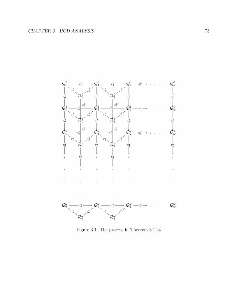
CHAPTER 3. HOD ANALYSIS 73
Q00 Q0
1 Q02 . . . Q0
ω
R00 R0
1
Q10 Q1
1 Q12 . . . Q1
ω
R10 R1
1
Q20 Q2
1 Q22 . . . Q2
ω
R20 R2
1
. . . .
. . . . . .
. . . . . .
. .
Qω0 Qω1 Qω2 . . . Qωω
Rω0 Rω
1
π00
σ00 j00
π01
σ01 j01
π02
π10
σ10 j10
π11
σ11 j11
π12
τ00
k00
τ01
k01
τ02 τ0
ω
π20
σ20 j20
π21
σ21 j21
π22
τ10
k10
τ11
k11
τ12 τ1
ω
τ20
k20
τ21
k21
τ22 τ2
ω
πω0
σω0 jω0
πω1
σω1 jω1
πω2
Figure 3.1: The process in Theorem 3.1.24
CHAPTER 3. HOD ANALYSIS 74
As in the previous lemma, we take a minimal such N and let Ω = P(R)N . We thenget N V = KΣ(R) and a (Q,Λ) with the property that Q ZFC\Powerset, Q ispointwise definable from ΣQ− , has ω Woodin cardinals above Q−. Furthermore, Λ is Ω-fullness preserving and for all B ∈ B(P,Σ)N , there is a Λ iterate (R,ΛR) of Q such that ΛRhas strong B-condensation. (Q,Λ) also has the property that any Λ iterate R of Q can befurther iterated by ΛR to S such that N is the derived model of S.
Fix 〈αi | i < ω〉 a cofinal in ΘΩ sequence of ordinals. Such a sequence exists sinceΩ = Env((Σ2
1)N). For each n, let
Dn = (R,Ψ, x, y) | (R,Ψ) is a hod pair equivalent to (P ,Σ), x codes R,y ∈ the least ODN
Ψ set of reals with Wadge rank ≥ αn
Clearly, for all n, Dn ∈ B(P ,Σ)N . By replacing (Q,Λ) by its appropriate iterate, we may
assume Λ has strong Dn-condensation for all n. Let ~D = 〈Dn | n < ω〉. Before proving thenext claim, let us introduce some notation. First let for a set A(A ⊆ R or A ∈ B(P ,Σ)),τQ,0A,m be the canonical capturing term for A in Q at (δ+m
0 )Q. Set
γQ,0Di,m= supHQ1 (P ∪ τQ,0Di,m
) ∩ δ0;γQ,0Di
= supm<ωγQ,0Di,m
.
Claim 1. For any Λ-iterate (S,Υ) of Q. Suppose i : Q → S is the iteration map. Then
i(δ0) = supi<ωγS,0Di.
Proof. Working in N , let 〈Ai | i < ω〉 be a sequence of ODΣ sets such that A0 is a universalΣ2
1(Σ) set; A1 = R\A0; the 〈Ai | i ≥ 2〉 is a semiscale on A1 (note that 〈Ai | i ≥ 2〉 is Wadgecofinal in Ω). Suppose φi and si ∈ OR<ω are such that
x ∈ Ai ⇔ N φi[Σ, si, x]
Now for each i, let
A∗i = (R,Ψ, x, y) | (R,Ψ) is a hod pair equivalent to (P ,Σ), x codes R,N φi[Ψ, si, y]
By the choice of the Ai’s (or just by the fact that Q is pointwise definable (over Q) fromΣQ−), we get
δ0 = supi<ωγQ,0A∗i.
By arguments in [26], we get that Λ is guided by 〈Ai | i < ω〉 for stacks above Q− andbelow δ0. This is just a straightforward adapatation of the proof of a similar fact in the caseΘ = θ0. This fact in turns implies
δ0 = supi<ωγQ,0Di.
CHAPTER 3. HOD ANALYSIS 75
To see this, fix an A∗i . We’ll show that there is a j such that γQ,0Dj≥ γQ,0A∗i
. Well, fix a realcoding P and let j be such that
w(Ai) = w((A∗i )(P,Σ,x)) ≤ w((Dj)(P,Σ,x)).
Let z be a real witnessing the reduction. Then there is a map i : Q → R such that
1. i is according to Λ and the iteration is above Q− = P ;
2. z is generic for the extender algebra A of R at δR.
Note that i(τQA∗i ) = τRA∗i , i(τQDj
) = τRDj , and R[z] τA∗i ≤w τDj via z. Hence τRA∗i ∈ X =
τ ∈ RA | (∃p ∈ A)(p R τ ≤w τDj via z) and |X|R < δR (by the fact that the extender
algebra A is δR-cc). But X is definable over R from τRDj , hence |X|R < γR,0Dj. Since τRA∗i ∈ X,
γR,0A∗i≤ γR,0Dj
which in turns implies γQ,0A∗i≤ γQ,0Dj
.
Now to finish the claim, let (S,Υ) be a Λ iterate of Q. Suppose i : Q → S is the iterationmap. Let R = i(P) and ΣQ be the tail of Σ under the iteration. We claim that
i(δ0) = supi<ωγS,0Di.(∗)
This is easily seen to finish the proof of Claim 1. To see (*), we repeat the proof of theprevious part applied to (S,Υ) and 〈Bi | i < ω〉 where B0 is a universal Σ2
1(ΣQ); B1 = R\B0;〈Bi | i ≥ 2〉 is a semiscale on B1. We may assume (S,Υ) is guided by 〈Bi | i < ω〉 for stacksabove R and below i(δ0). Now we are in the position to apply the exact same argument asabove and conclude that (*) holds. Hence we’re done.
Since Λ has the Dodd-Jensen property, the direct limit M∞(Q,Λ) of Λ-iterates of Qbelow δQ0 is defined and is wellfounded (note that we allow iterations based on Q−). Let〈δQi | i < ω〉 be the first ω Woodins of Q above Q− and iQ,ΛQ,∞ : Q → M∞(Q,Λ) be the
direct limit embedding. For (R,ΛR), an iterate of (Q,Λ) below δQ0 , let iR,ΛRR,∞ have the ob-
vious meaning and iQ,ΛQ,R be the iteration map according to Λ. By a similar argument as
in the computation of HODL(R), we get 〈ηn | n < ω〉 = 〈iQ,ΛQ,∞(δQi ) | i < ω〉. Also in N ,M∞(Q,Λ)|ηn = M∞|ηn for all n and hence M∞ = M∞(Q,Λ)|supn<ωηn. In particular,M∞ is wellfounded.
Working in N , we first claim that
Claim 2. M∞(Q,Λ)|η0 = V HODη0
. (*)
Proof. To show (*), it is enough to show that if A ⊆ α < η0 and A is OD then A ∈M∞(Q,Λ). To see this, let i be such that γ
M∞(Q,Λ),0Di
> α (such an i exists by the proof ofClaim 1). Let
C = (R,Ψ, x, y) | (R,Ψ) is a hod pair equivalent to (P ,Σ), x codes R, y codes (N, γ)
such that (N ,Ψ) is 1-suitable, N is strongly Di iterable via a
quasi-strategy Φ extending Ψ, γ < γN ,0Di, π
(N ,Ψ),∞Di
(γ) ∈ A.
CHAPTER 3. HOD ANALYSIS 76
By replacing Q by an iterate we may assume (Q,Λ) is C-iterable. Let τQC = τQC,(δ+ω
0 )Qand
τC = i(Q,Λ)Q,∞ (τQC ). The following equivalence is easily shown by a standard computation:
ξ ∈ A iff M∞(Q,Λ) Col(ω,η+ω0 ) “if x codes iQ,ΛQ,∞(P), y codes (M∞(Q,Λ)|η+ω
0 , ξ)
then (x, y) ∈ τC”.
For the reader’s convenience, we’ll show why the above equivalence holds. First supposeξ ∈ A. Let (S,Ξ) ∈ I(Q,Λ) be such that there is a γ < γS,0Di
and iS,ΞS,∞(γ) = ξ. Then we have
(letting ν = iQ,ΛQ,S(δ0))
S Col(ω,ν+ω) “if x codes iQ,ΛQ,S(P), y codes (S|ν+ω, γ) then (x, y) ∈ iQ,ΛQ,S(τQ,ΛC )”.
By applying iS,ΞS,∞ to this ,we get
M∞(Q,Λ) Col(ω,η+ω0 ) “if x codes iQ,ΛQ,∞(P), y codes (M∞(Q,Λ)|η+ω
0 , ξ) then (x, y) ∈ τC”.
Now to show (⇐), let (S,Ξ) ∈ I(Q,Λ) be such that for some γ < γS,0Di, ξ = iS,ΞS,∞(γ). Let
ν = iQ,ΛQ,S(δ0), we have
S Col(ω,ν+ω) “if x codes iQ,ΛQ,S(P), y codes (S|ν+ω, γ) then (x, y) ∈ iQ,ΛQ,S(τQ,ΛC )”.
This means there is a quasi-strategy Ψ on S(0) (S(0) = S|(ν+ω)S) such that (S(0), iQ,ΛQ,S(Σ)) is
1-suitable, Ψ extends iQ,ΛQ,S(Σ)), and Ψ is Di-iterable. We need to see that π(S(0),iQ,ΛQ,S(Σ)),∞Di
(γ) =
ξ. But this is true by the choice of Di, ξ = iS,ΞS,∞(γ), and the fact that Ψ agrees with Ξ on
how ordinals below γS,0Diare mapped.
The equivalence above shows A ∈M∞(Q,Λ), hence completes the proof of (*).
(*) in turns shows that η0 is a cardinal in HOD and η0 ≤ Θ (otherwise, HOD|η0 =M∞(Q,Λ)|η0 Θ is not Woodin while HOD Θ is Woodin). Next we show
Claim 3. η0 = Θ. (∗∗)
Proof. Suppose toward a contradiction that η0 < Θ. Let Q(0) = Q|(δ+ω0 )Q, Λ0 = Λ|Q(0),
and M∞(Q,Λ)(0) = M∞(Q,Λ)|(η+ω0 )M∞(Q,Λ). Let π = i Q(0); so π is according to Λ0.
By the Coding Lemma and our assumption that η0 < Θ, π,M∞(Q,Λ)(0) ∈ N . From this,
we can show Λ0 ∈ N by the following computation: Λ0(~T ) = b if and only if
1. the part of ~T based on P is according to Σ;
2. if i~Tb exists then there is a σ :M~T
b →M∞(Q,Λ)(0) such that π = σ i~Tb ;
CHAPTER 3. HOD ANALYSIS 77
3. ~T aM~Tb is Q-structure guided.
By branch condensation of Λ0, (1),(2), and (3) indeed define Λ0 in N . This means Λ0 isODN from Σ (and some real x); hence Λ0 ∈ N . So suppose γ = w(Code(Λ0)) < ΘΩ. In N,let
B = (R,Ψ, x, y) | (R,Ψ) is a hod pair equivalent to (P ,Σ), x codes R, y ∈ ARwhere AR is the least OD(Code(Ψ)) set such that w(AR) > γ
and AR is not projective in any set with Wadge rank γ
Then B ∈ B(P ,Σ)N . We may assume Λ0 respects B. It is then easy to see that whenever(R,ΛR) ∈ I(Q(0),Λ0) (also let S / R be the iterate of P), AR is projective in Code(ΛR)(and hence AR is projective in Code(Λ0)) because ΛR can compute membership of AR byperforming genericity iterations (above S) to make reals generic. This contradicts the choiceof AR.
Claims 2 and 3 complete the proof of the lemma.
Now we define a strategy Σ∞ for M∞ extending the strategy Σ−∞ of M−∞ = V HOD
θα. Let
(P ,Σ, A) ∈ F and suppose P is n-suitable with 〈δi | i < n〉 being the sequence of Woodins ofP above P−, let τM∞A,k = common value of πP,Σ~B,∞
(τPA,δk). Σ∞ will be defined (in V) for trees on
M∞|η0 in M∞. For k ≥ n, M∞ ”Col(ω, ηn)× Col(ω, ηk) (τM∞A,n )g = (τM∞A,k )h ∩M∞[g]”
where g is Col(ω, ηn) generic and h is Col(ω, ηk) generic and (τM∞A,n )g is understood to beA(M−∞,Σ−∞) ∩M∞[g]. This is just saying that the terms cohere with one another.
Let λM∞ = supi<ωηi. LetG be Col(ω, λM∞) generic overM∞. Then R∗G is the symmetricreals and A∗G := ∪k(τM∞A,k )G|ηk .
Proposition 3.1.27. For all A ∈ B(M−∞,Σ
−∞), L(A∗G,R∗G) AD+
Proof. We briefly sketch the proof of this since the techniques involved have been fully spelledout before. If not, reflect the situation down to a model N coded by a Suslin co-Suslin set.Next get a “next mouse” N with ω Woodin cardinals that iterates out to (possibly a longermouse than)MN
∞. N also has the property that its derived model is elementarily equivalentto N .
Let A ⊆ B(M−∞,Σ
−∞) be the least OD set such that L(A∗G,R∗G) 2 AD+. Then there is
an iterate M of N having preimages of all the terms τM∞A,k . We may assume M has derived
model KΣ(R) and suitable initial segments ofM are in FN . Since we have AD+,M thinksthat its derived model (in this case is KΣ(R)) satisfies that L(A(P,Σ),R) AD+, where wereuse (P ,Σ) for an equivalent (but possibly different) hod pair from the original one. NowiterateM to Q such thatM∞ is an initial segment of Q. By elementarity L(A∗G,R∗G) AD+.This is a contradiction.
CHAPTER 3. HOD ANALYSIS 78
Definition 3.1.28. Given a normal tree T ∈ M∞ and T is based on M∞|θ0. T is by Σ∞if the following hold (the definition is similar for finite stacks):
• If T is short then Σ picks the branch guided by Q-structure (as computed in M∞).
• If T is maximal then Σ∞(T ) = the unique cofinal branch b which moves τM∞A,0 correctly
for all A ∈ OD such that there is some (P ,Σ, A) ∈ F i.e. for each such A, ib(τM∞A,0 ) =
τMTbA∗,0.
Lemma 3.1.29. Given any such T as above, Σ∞(T ) exists.
The proof of the lemma is similar to the proof of Lemma 3.1.14. So we omit it.It is evident that L(M∞,Σ∞) ⊆ HOD. Next, we show M∞ and Σ∞ capture all un-
bounded subsets of Θ in HOD. In L(M∞,Σ∞), first construct (using Σ∞) a mouse M+∞
extending M∞ such that o(M∞) is the largest cardinal of M+∞ as follows:
1. Let R∗G be the symmetric reals obtained from a generic G overM∞ of Col(ω,< λM∞).
2. For each A∗G (defined as above) (we know L(R∗G, A∗G) AD+), pull back the hybrid miceover R∗G in this model to hybrid mice S extendingM∞ with D(S, λM∞) = L(R∗G, A∗G).
3. Let M+∞ = ∪SS for all such S above. M+
∞ is independent of G. By a reflectionargument (and Prikry-like forcing) as above, the translated mice over M∞ are allcompatible, no levels of M+
∞ projects across o(M∞), and M+∞ contains as its initial
segments all translation of R∗G-mice in D(M+∞, λ
M∞). This is just saying that M+∞
contains enough mice to compute HOD.
Remark 3.1.30. Θ is not collapsed by Σ∞ as it is a cardinal in HOD. Σ∞ is used to obtainthe A∗G above by moving correctly the τM∞A,0 in genericity iterations. L(M∞) does not see
the sequence 〈τM∞A,k |k ∈ ω〉 hence can’t construct A∗G. Also since Σ∞ collapses δM∞1 , δM∞2 ...,it doesn’t make sense to talk about D(L(M∞,Σ∞)).
Lemma 3.1.31. HOD ⊆ L(M∞,Σ∞)
Proof. Using Theorem 3.1.9, we know HOD = L[P ] for some P ⊆ Θ. Therefore, it is enoughto show P ∈ L(M∞,Σ∞). Let φ be a formula defining P , i.e.
α ∈ P ⇔ V φ[α].
We suppress the ordinal parameter here. Now in L(M∞,Σ∞) let π : M∞|(η++0 )M∞ →
(M∞)(M+∞,λM∞ ) where π is according to Σ∞.
Claim: α ∈ P ⇔ D(M+∞, λ
M∞) φ[π(α)]. (*)

CHAPTER 3. HOD ANALYSIS 79
Proof. Otherwise, reflect the failure of (*) as before to get a model N coded by a Suslinco-Suslin set, a hod pair (P ,Σ) giving us HOD|θα such that
N ZF + DC + AD+ + V = KΣ(R) + (∃α)(φ[α] < D(M+∞,Σ∞) φ[π(α)]).
Fix such an α. As before, let N be the next mouse (i.e. N has ω Woodins 〈δi | i < ω〉 ontop of P) with ρ(N ) < supiδi) with strategy Λ extending Σ and Λ has branch condensation
and is Ω-fullness preserving, where Ω = (Σ21)N . We may assume Λ is guided by ~D where
~D = 〈Dn | n < ω〉 is defined as in Lemma 3.1.26. As before, we may assume N has derivedmodel N . Let σ : N |((δN0 )++)N → (M∞)D(N,λN ) be the direct limit map by Λ. We mayassume σ(α) = α for some α. Working in N , it then remains to see that:
D(M+∞, λ
M∞) φ[π(α)]⇔ D(N, λN) φ[σ(α)] (∗∗).
To see that (**) holds, we need to see that the fragment of Λ that defines σ(α) can be definedin D(N, λN). This then will give the equivalence in (**). Because α < η0, α < δ0, pick an nsuch that such that γN,0Dn,0
> α. Then the fragment of Λ that defines σ(α) is definable from
Dn (and N |(δN0 )) in D(N, λN), which is what we want.The equivalence (**) gives us a contradiction.
The claim finishes the proof of P ∈ L(M∞,Σ∞). This then implies HOD = L[P ] ⊆L(M∞,Σ∞).
Lemma 3.1.31 implies HOD = L(M∞,Σ∞), hence completes our computation.
3.1.2 The Limit Case
There are two cases: the easier case is when HOD “cof(Θ) is not measurable”, and theharder case is when HOD “cof(Θ) is measurable”.
Here’s the direct limit system that gives us V HODΘ .
F = (Q,Λ) | (Q,Λ) is a hod pair; Λ is fullness preserving and has branch condensation.
The order on F is given by
(Q,Λ) ≤F (R,Ψ) ⇔ Q iterates to a hod initial segment of R.
By Theorem 1.2.2, ≤F is directed and we can form the direct limit of F under the naturalembeddings coming from the comparison process. Let M∞ be the direct limit. By thecomputation in [23],
|M∞| = V HODΘ .
M∞ as a structure also has a predicate for its extender sequence and a predicate for asequence of strategies.
We quote a theorem from [23] which will be used in the upcoming computation. Forunexplained notations, see [23].
CHAPTER 3. HOD ANALYSIS 80
Theorem 3.1.32 (Sargsyan, Theorem 4.2.23 in [23]). Suppose (P ,Σ) is a hod pair such thatΣ has branch condensation and is fullness preserving. There is then Q a Σ-iterate of P suchthat whenever R is a ΣQ-iterate of Q, α < λR, and B ∈ (B(R(α),ΣR(α)))
L(Γ(R(α+1),ΣR(α+1)))
1. ΣR(α+1) is super fullness preserving and is strongly guided by some
~B = 〈Bi | i < ω〉 ⊆ (B(R(α),ΣR(α)))L(Γ(R(α+1),ΣR(α+1)));
2. there is a (S,ΣS) ∈ I(R(α + 1),ΣR(α+1)) such that ΣS has strong B-condensation.
We deal with the easy case first.
3.1.2.1 Nonmeasurable Cofinality
The following theorem is the full HOD computation in this case.
Theorem 3.1.33. HOD = L(M∞)
Proof. To prove the theorem, suppose the equality is false. Then by Theorem 3.1.9, thereis an A ⊆ Θ such that A ∈ HOD\L(M∞) (the fact that L(M∞) ⊆ HOD is obvious). ByΣ1-reflection (i.e. Theorem 1.1.5), there is a transitive N coded by a Suslin co-Suslin setsuch that
N ZF− + AD+ + V = L(P(R)) + SMC + Θ exists and is limit in the Solovay sequence
+HOD “cof(Θ) is not measurable ” + “∃B ⊆ Θ(B ∈ HOD\L(M∞))”.
Take N to be the minimal such and let B witness the failure of the theorem in N . Let φdefine B (for simplicity, we suppress the ordinal parameter) i.e.
α ∈ B ⇔ N φ[α]
Let Ω = P(R)N . There is a pair (P ,Σ) such that:
1. P = Lβ(∪γ<λPPγ) for some λP ;
2. for all γ < λP , Pβ is a hod mouse whose strategy Σγ ∈ Ω is Ω-fullness preserving, hasbranch condensation, and λPβ = β;
3. if γ < η < λP , Pγ hod Pη;
4. β is least such that ρω(Lβ(∪γ<λPPγ)) < o(∪γ<λPPγ));
5. P cof(λP) is not measurable;
6. Σ has branch condensation and extends γ<λPΣγ;
CHAPTER 3. HOD ANALYSIS 81
Such a (P ,Σ) can be obtained by performing a Ω-hod pair construction (see Definition1.2.9) inside some N∗x capturing a good pointclass beyond Ω. We may and do assume that(∪γ<λPPγ,γ<λPΣγ) satisfies Theorem 3.1.32 applied in N . This implies that the directlimitM+
∞ of all Σ-iterates of P is a subset of HODN . Let j : P →M+∞ be the natural map.
Then in N , M+∞|j(λP) =M∞.
Now pick a sequence 〈γi | i < ω〉 cofinal in λP such that δλPγi is Woodin in P , anenumeration 〈xi | i < ω〉 of R and do a genericity iteration of P to successively make each xigeneric at appropriate image of δλPγi . Let Q be the end model of this process and i : P → Qbe the iteration embedding. Then by assumption (5) above, we have that N is the derivedmodel of Q at i(λP ).
In N , let D be the derived model of M+∞ at Θ and
π∞ :M∞ → (M∞)D
be the direct limit embedding given by the join of the strategies ofM∞’s hod initial segments.Then by the same argument as that given in Lemma 3.1.16, we have
α ∈ B ⇔ D φ[π∞(α)].
The proof of Lemma 3.1.16 also gives that B ∈ (L(M∞))N , which contradicts our assump-tion. Hence we’re done.
Remark 3.1.34. It’s not clear that in the statement of Theorem 3.1.33, “M∞” can bereplaced by “V HOD
Θ ”.
3.1.2.2 Measurable Cofinality
Suppose HOD cof(Θ) is measurable. We know by [23] that V HODΘ is |N∞| where N∞ is
the direct limit (under the natural maps) of F , where F is introduced at the beginning ofthis section. Let
M∞ = Ult0(HOD, µ)|Θ,
where µ is the order zero measure on cofHOD(Θ). Let f : cofHOD(Θ) =def α → Θ be acontinuous and cofinal function in HOD. For notational simplicity, for each β < α, let Λβ bethe strategy of M∞(f(β)) and Σβ be the strategy of N∞(f(β)). Let
M+∞ = Ult0(HOD, µ)|(Θ+)Ult0(HOD,µ),
and
N+∞ = ∪M | N∞ EM, ρ(M) = Θ,M is a hybrid mouse satisfying property (*).
Here a mouse M satisfies property (*) if whenever π : M∗ → M is elementary, M∗ iscountable, transitive, and π(Θ∗) = Θ, then M∗ is a ⊕ξ<Θ∗Σ
∗ξ-mouse for stacks above Θ∗,
CHAPTER 3. HOD ANALYSIS 82
where Σ∗ξ is the strategy for the hod mouse M∗(ξ) obtained by the following process: let(P ,Σ) ∈ F and i : P → M∞ be the direct limit embedding such that the range of icontains the range of π M∗(ξ); Σ∗ξ is then defined to be the π i−1-pullback of Σ. It’seasy to see that the strategy Σ∗ξ as defined doesn’t depend on the choice of (P ,Σ). This isbecause if (P0,Σ0, i0) and (P1,Σ1, i1) are two possible choices to define Σ∗ξ , we can coiterate(P0,Σ0) against (P1,Σ1) to a pair (R,Λ) and let ii : Pi → R be the iteration maps andlet i2 : R → M∞ be the direct limit embedding. Then Σ0 = Λi0 and Σ1 = Λi1 ; hence theπ i−1
0 -pullback of Σ0 is the same as the π i−11 -pullback of Σ1 because both are the same
as the π i−12 -pullback of Λ.
We give two characterizations of HOD here: one in terms ofM+∞ and the other in terms
of N+∞. The first one is easier to see.
Theorem 3.1.35. 1. HOD = L(N∞,M+∞).
2. HOD = L(N+∞).
Proof. To prove (1), first let jµ : HOD → Ult0(HOD, µ) be the canonical ultrapower map.Let A ∈ HOD, A ⊆ Θ. By the computation of HOD below Θ, we know that for each limitβ < α,
A ∩ θf(β) ∈ |N∞(f(β))|.This means
jµ(A) ∩Θ ∈M+∞.
We then have
γ ∈ A⇔ jµ(γ) ∈ jµ(A) ∩Θ.
Since jµ|Θ agrees with the canonical ultrapower map k : N∞ → Ult0(N∞, µ) on all ordinalsless than Θ, the above equivalence shows that A ∈ L(N∞,M+
∞). This proves (1).Suppose the statement of (2) is false. There is an A ⊆ Θ such that A ∈ HOD\N+
∞. ByΣ1-reflection (i.e. Theorem 1.1.5), there is a transitive N coded by a Suslin co-Suslin setsuch that
N ZF− + DC + V = L(P(R)) + SMC + “Θ exists and is limit in the Solovay sequence ”
+“HOD cof(Θ) = α is measurable as witnessed by f”
+“∃A ⊆ Θ(A ∈ HOD\N+∞)”.
Take N to be the minimal such and let A witness the failure of (2) in N . Let µ, jµ,M∞, M+
∞, N∞, N+∞ be as above but relativized to N . Working in N , there is a sequence
〈Mβ | β < α, β is limit〉 ∈ HOD such that for each limit β < α, Mβ is the least hod initialsegment of N∞|θf(β) such that A ∩ θf(β) is definable over Mβ.
Let Ω = P(R)N . Fix an N∗x capturing a good pointclass beyond Ω. Now, we again dothe Ω-hod pair construction in N∗x to obtain a pair (Q,Λ) such that
CHAPTER 3. HOD ANALYSIS 83
1. there is a limit ordinal λQ such that for all γ < λQ, Qβ is a hod mouse with λQβ = βand whose strategy Ψγ ∈ Ω is Ω-fullness preserving, has branch condensation;
2. if γ < η < λQ, Qγ hod Qη;
3. Q is the first sound mouse from the L[E,γ<λQΨγ][∪γ<λQQγ]-construction done in N∗xthat has projectum ≤ o(∪γ<λQQγ) and extends LpΩ,
γ<λQΨγ (∪γ<λQQγ) 10 and Λ bethe induced strategy of Q.
From the construction of Q and the properties of N , it’s easy to verify the following:
1. Let δλQ = o(∪γ<λQQγ) and η = o(LpΩ,γ<λQΨγ (∪γ<λQQγ)). Then η = (δ+
λQ)Q.
2. Λ /∈ Ω.
3. Q δλQ has measurable cofinality.
Let M∞(Q,Λ) be the direct limit (under natural embeddings) of Λ-iterates of Q.
Lemma 3.1.36. M∞(Q,Λ) exists.
Proof. First note that Λ is Ω-fullness preserving. To see this, suppose not. Let k : Q → R beaccording to Λ witnessing this. It’s easy to see that the tail ΛR of Λ acting on R|k(η) is notin Ω (otherwise, Λk
R = Λ by hull condensation and hence Λ ∈ Ω. Contradiction.) However,γ<λRΨR(γ) ∈ Ω since the iterate of N∗x by the lift-up of k thinks that the fragment of itsstrategy inducing γ<λRΨR(γ) is in Ω. Now suppose M is a γ<λRΨR(γ)-mouse projectingto δλR with strategy Ξ in Ω and M 5 R (again, Ξ acts on trees above δλR and moves thepredicates for γ<λRΨR(γ) correctly). We can compare M and R (the comparison is aboveδλR). Let M be the last model on the M side and R on the R side. Then R M. Letπ : R → R be the iteration map from the comparison process and Σ be the π k-pullbackof the strategy of R. Hence Σ ∈ Ω since Ξ ∈ Ω. Σ acts on trees above δλQ and movesthe predicate for γ<λQΨγ correctly by by our assumption on Ξ and branch condensation
of γ<λQΨγ. These properties of Σ imply that Q LpΩ,γ<λQΨγ (∪γ<λQQγ). Contradiction.
For the case that there are α < λR, δRα ≤ η < δRη+1, and η is a strong cutpoint of R, andMis a sound ΨR(α)-mouse projecting to η with iteration strategy in Ω, the proof is the sameas that of Theorem 3.7.6 in [23].
Now we show Λ has branch condensation (see Figure 3.2). The proof of this comes fromprivate conversations between the author and John Steel. We’d like to thank him for this.For notational simplicity, we write Λ− for γ<λQΨγ. Hence, Λ /∈ Ω and Λ− ∈ Ω. SupposeΛ does not have branch condensation. We have a minimal counterexample as follows: thereare an iteration i : Q → R by Λ, a normal tree U on R in the window [ξ, γ) where ξ < γ
10If M LpΩ,γ<λQΨγ (∪γ<λQQγ) and M extends ∪γ<λQQγ then M is a mouse in N in the sense thatN knows how to iterate M for stacks above o(∪γ<λQQγ).
CHAPTER 3. HOD ANALYSIS 84
are two consecutive Woodins in R such that supi′′δλQ ≤ ξ, two distinct cofinal branches ofU : b and c = ΛR(U), an iteration map j : Q → S by Λ, and a map σ :MU
b → S such thatj = σ iUb i. We may also assume that if R is the first model along the main branch ofthe stack from Q to R giving rise to i and iR,R : R → R be the natural map such that
iR,R(ξ) = ξ and iR,R(γ) = γ, then the extenders used to get from Q to R have generators
below ξ. This gives us sup(HullR(ξ ∪ p) ∩ γ) = γ where p is the standard parameter ofR. Let Φ = Λσ
S and Φ− = ⊕ξ<λ
MUb
ΦMUb (ξ). It’s easy to see that Φ− ∈ Ω. By the same proof
as in the previous paragraph, Φ is Ω-fullness preserving. This of course implies that MUb is
Ω-full and Φ /∈ Ω.Now we compareMU
b andMUc . First we line up the strategies ofMU
b |δ(U) andMUc |δ(U)
by iterating them into the (Ω-full) hod pair construction of some N∗y (where y codes (x,MUc ,
MUb )). This can be done because the strategies of MU
b |δ(U) and of MUc |δ(U) have branch
condensation by Theorems 2.7.6 and 2.7.7 of [23]11. This process produces a single normaltreeW . Let a = Φ(W) and d = ΛMUc (W). Let X = HullR(ξ∪p)∩γ. Note that (iWa iUb )”X⊆ δ(W) and iWd iUc ”X ⊆ δ(W). Now continue lining up MW
a and MWd above δ(W) (using
the same process as above). We get π : MWa → K and τ : MW
d → K (we indeed end upwith the same model K by our assumption on the pair (Λ,Λ−)). But then
(π iWa iUb )”X = (τ iWd iUc )”X.
But by the fact that (iWa iUb )”X ⊆ δ(W) and iWd iUc ”X ⊆ δ(W) and π agrees with τ aboveδ(W), we get
(iWa iUb )”X = (iWd iUc )”X.
This gives ran(iWa ) ∩ ran(iWd ) is cofinal in δ(W), which implies a = d. This in turns easilyimplies b = c. Contradiction. Finally, let R and S be Λ-iterates of Q and let ΛR and ΛSbe the tails of Λ on R and S respectively. We want to show that R and S can be furtheriterated (using ΛR and ΛS respectively) to the same model. To see this, we compare Rand S against the Ω-full hod pair construction of some N∗y (for some y coding (x,R,S)).Then during the comparison, only R and S move (to say R∗ and S∗). It’s easy to see thatR∗ = S∗ and their strategies are the same (as the induced strategy of N∗y on its appropriatebackground construction).
By the properties of (Q,Ψ) and Λ, we get that ρ(M∞(Q,Λ)) ≤ Θ and (HOD|Θ)N =M∞(Q,Λ)|Θ. Let k be the least such that ρk+1(Q) ≤ δλQ .
Claim. M∞(Q,Λ) /∈ N11We note here that suppose (P,Σ) is a hod pair and P δP has measurable cofinality. Then knowing
that all “lower level” strategies of all iterates of (P,Σ) has branch condensation does not tell us that Σ itselfhas branch condensation.
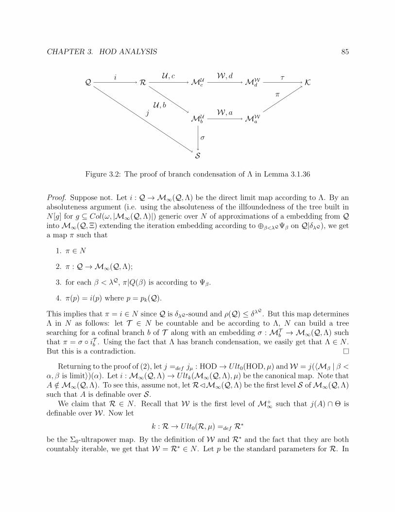
CHAPTER 3. HOD ANALYSIS 85
Q R MUc MW
d K
MUb MW
a
S
i U , c W , d τ
U , bW , a
π
j
σ
Figure 3.2: The proof of branch condensation of Λ in Lemma 3.1.36
Proof. Suppose not. Let i : Q →M∞(Q,Λ) be the direct limit map according to Λ. By anabsoluteness argument (i.e. using the absoluteness of the illfoundedness of the tree built inN [g] for g ⊆ Col(ω, |M∞(Q,Λ)|) generic over N of approximations of a embedding from QintoM∞(Q,Ξ) extending the iteration embedding according to β<λQΨβ on Q|δλQ), we geta map π such that
1. π ∈ N
2. π : Q →M∞(Q,Λ);
3. for each β < λQ, π|Q(β) is according to Ψβ.
4. π(p) = i(p) where p = pk(Q).
This implies that π = i ∈ N since Q is δλQ-sound and ρ(Q) ≤ δλQ
. But this map determinesΛ in N as follows: let T ∈ N be countable and be according to Λ, N can build a treesearching for a cofinal branch b of T along with an embedding σ :MT
b →M∞(Q,Λ) suchthat π = σ iTb . Using the fact that Λ has branch condensation, we easily get that Λ ∈ N .But this is a contradiction.
Returning to the proof of (2), let j =def jµ : HOD→ Ult0(HOD, µ) andW = j(〈Mβ | β <α, β is limit〉)(α). Let i :M∞(Q,Λ)→ Ultk(M∞(Q,Λ), µ) be the canonical map. Note thatA /∈M∞(Q,Λ). To see this, assume not, letRM∞(Q,Λ) be the first level S ofM∞(Q,Λ)such that A is definable over S.
We claim that R ∈ N . Recall that W is the first level of M+∞ such that j(A) ∩ Θ is
definable over W . Now let
k : R → Ult0(R, µ) =def R∗
be the Σ0-ultrapower map. By the definition of W and R∗ and the fact that they are bothcountably iterable, we get that W = R∗ ∈ N . Let p be the standard parameters for R. In
CHAPTER 3. HOD ANALYSIS 86
N , we can compute ThR0 (Θ ∪ p) as follows: for a formula ψ in the language of hod premiceand s ∈ Θ<ω,
(ψ, s) ∈ ThR0 (Θ ∪ p)⇔ (ψ, j(s)) ∈ ThR∗0 (Θ ∪ k(s)).
Since ThR∗
0 (Θ ∪ k(s)) = ThW0 (Θ ∪ k(s)) ∈ N , j|Θ ∈ N , and k(s) ∈ W ∈ N , we getThR0 (Θ ∪ p) ∈ N . This shows R ∈ N .
To get a contradiction, we show R N+∞ by showing R is satisfies property (*) in N .
Let K be a countable mouse embeddable into R by a map k ∈ N . Then we can compareK and Q against the Ω-full hod pair construction of some N∗y just like in the argument onthe previous page; hence we may assume KQ (QK can’t happen because then Λ ∈ N).The minimality assumption on Q easily implies K LpΩ,
γ<λQΨγ (Q|δλQ). But then N caniterate K for stacks on K above δλQ = δλK , which is what we want to show. The fact thatRN+
∞ contradicts A /∈ N+∞.
Next, we note that Ult0(HOD, µ)|Θ = Ultk(M∞(Q,Λ), µ)|Θ and i|Θ = j|Θ. LetR = ThM∞(Q,Λ)(Θ ∪ p) where p = pk(M∞(Q,Λ)) and S = ThUltk(M∞(Q,Λ),µ)(Θ ∪ i(p)).We have that Mα and S are sound hybrid mice in the same hierarchy, hence by countableiterability, we can conclude either Mα C S or S Mα.
If Mα C S, then Mα ∈ Ultk(M∞(Q,Λ), µ). This implies A ∈ M∞(Q,Λ) by a compu-tation similar to that in the proof of (1), i.e.
β ∈ A⇔M∞(Q,Λ) (i|Θ)(β) ∈Mα.
This is a contradiction to the fact that A /∈ M∞(Q,Λ). Now suppose S Mα. Thisthen implies S ∈ Ult0(HOD, µ), which in turns implies M∞(Q,Λ) ∈ HOD by the followingcomputation: for any formula φ and s ∈ Θ<ω,
(φ, s) ∈ R ⇔ HOD (φ, (j|Θ)(s)) ∈ S.
This is a contradiction to the claim. This completes the proof of (2).
Theorem 3.1.35 completes our analysis of HOD for determinacy models of the form“V = L(P(R)) below “ADR + Θ is regular.”
3.2 When V = L(R, µ)
We prove the case α = 0. The other cases are similar. Throughout this section, we assumeL(R, µ) AD+ + µ is a normal fine measure on Pω1(R). We’ll be using the following theorem.
Theorem 3.2.1 (Woodin). Suppose L(R, µ) AD+ +µ is a normal fine measure on Pω1(R).Then in L(R, µ), there is a set A ⊆ Θ such that HOD = L[A].
CHAPTER 3. HOD ANALYSIS 87
3.2.1 HODL(R,µ) with M]ω2
We assume µ comes from the club filter,M]ω2 exists and has Hom∞ iteration strategy. We’ll
show how to get rid of these assumptions later on. We first show how to iterate Mω2 torealize µ as the tail filter.
Lemma 3.2.2. There is an iterate N ofMω2 such that letting λ be the limit of N ’s Woodincardinals, R can be realized as the symmetric reals over N at λ and letting F be the tail filterover N at λ, L(R, µ) = L(R,F).
Proof. Let δi be the sup of the first ωi Woodin cardinals ofMω2 and γ = supi δi. Let ξ ≥ ω1
be such that H(ξ) ZFC−. In V Col(ω,H(ξ)), let 〈Xi | i < ω〉 be an increasing and cofinalchain of countable (in V ) elementary substructures of H(ξ) and σi = R ∩Xi. To constructthe N as in the statement of the lemma, we do an R-genericity iteration (in V Col(ω,H(ξ))) asfollows. Let P0 =M]
ω2 and assume P0 ∈ X0. For i > 0, let Pi be the result of iterating Pi−1
in Xi−1 in the window between the ω(i − 1)th and ωith Woodin cardinals of Pi−1 to makeσi−1 generic. We can make sure that each finite stage of the iteration is in Xi−1. Let Pω beobtained from the direct limit of the Pi’s and iterating the top extender out of the universe.Let λ be the limit of Woodin cardinals in Pω. It’s clear that there is a G ⊆ Col(ω,< λ)generic over Pω such that R =def RV is the symmetric reals over Pω and L(R, µ) is in Pω[G].Let F be the tail filter on Pω1(R) defined over Pω[G]. By section 2, L(R,F) F is a normalfine measure on Pω1(R).
We want to show L(R, µ) = L(R,F). To show this, it’s enough to see that if A ⊆ Pω1(R)is in L(R, µ) and A is a club then A ∈ F . Let π : R<ω → R ∈ V witness that A is a club. Bythe choice of the Xi’s, there is an n such that for all m ≥ n, π ∈ Xm and hence π′′σ<ωm ⊆ σm.This shows A ∈ F . This in turns implies L(R, µ) = L(R,F).
Let M+∞ be the direct limit of all iterates of Mω2 below the first Woodin cardinal and
H+ be the corresponding direct limit system. We’ll define a direct limit system H in L(R, µ)that approximates H+. Working in L(R, µ), we say P is suitable if it is full (with respectto mice), has only one Woodin cardinal δP and P = Lpω(P|δP). The following definitioncomes from Definition 6.21 in [41].
Definition 3.2.3. Working in L(R, µ), we let O be the collection of all functions f suchthat f is an ordinal definable function with domain the set of all countable, suitable P, and∀P ∈ dom(f)(f(P) ⊆ δP).
Definition 3.2.4. Suppose ~f ∈ O<ω, P is suitable, and dom(~f) = n. Let
γ(P, ~f) = supHullP(~f(0)(P), · · · , ~f(n− 1)(P)) ∩ δP,
andH(P, ~f) = HullP(γ(P, ~f) ∪ ~f(0)(P), · · · , ~f(n− 1)(P)).
CHAPTER 3. HOD ANALYSIS 88
We refer to reader to Section 6.3 of [41] for the definitions of ~f -iterability, strong ~f -iterability. The only difference between our situation and the situation in [41] is that ournotions of “suitable”, “short”, “maximal”, “short tree iterable” etc. are relative to thepointclass (Σ2
1)L(R,µ) instead of (Σ21)L(R) as in [41].
Now, let (P , ~f) ∈ H if P is strongly ~f -iterable. The ordering on H is defined as follows:
(P , ~f) ≤H (Q, ~g)⇔ ~f ⊆ ~g ∧Q is a psuedo-iterate of P12.
Note that if (P , ~f) ≤H (Q, ~g) then there is a natural embedding π(P, ~f),(Q,~q) : HP, ~f → HQ,~g.
We need to see that H 6= ∅.
Lemma 3.2.5. Let ~f ∈ O<ω. Then there is a P such that (P , ~f) ∈ H.
Proof. For simplicity, assume dom(~f) = 1. The proof of this lemma is just like the proof ofTheorem 6.29 in [41]. We only highlight the key changes that make that proof work here.
First let ν,P be as in the proof of Lemma 2.1.6. Let a be a countable transitive self-wellordered set and x be a real that codes a. We need to modify the Qx
a defined in the proofof Lemma 2.1.6 to the structure defined along the line of Subsection 3.1.1.1. Fix a coding ofrelativized premice by reals and write Pz for the premouse coded by z. Then let
Fxa = Pz | z ≤T x and Pz is a suitable premouse over a and Pz is short-tree iterable.
Let
Qxa = Lp(Qx,−a ),
where Qx,−a is the direct limit of the simultaneous comparison and y | y ≤T x-genericityiteration of all P ∈ Fxa . The definition of Qxa comes from Section 6.6 of [41]. As in the proofof Lemma 2.1.6, we have:
1. letting 〈~di | i < ω〉 be the generic sequence for P and 〈Qij | i, j < ω〉 be the sequence
of models associated to 〈~di | i < ω〉 as defined in the proof of Lemma 2.1.6, we
have that the model N = L[T∞,M〈~di〉i ] “there are ω2 Woodin cardinals”, where
M〈~di〉i = L[∪i ∪j Qij];
2. letting λ be the sup of the Woodin cardinals of N , there is a G ⊆ Col(ω,< λ), G isN -generic such that letting R∗G be the symmetric reals of N [G] and F be the tail filterdefined over N [G], then L(R∗G,F) = L(R, µ) and F ∩ L(R, µ) = µ.
The second key point is that whenever P is an iterate of Mω2 , we can then iterate P toQ (above any Woodin cardinal of P) so that RV can be realized as the symmetric reals forsome G ⊆ Col(ω,< δQω2) and L(R, µ) = L(R,F) and µ ∩ L(R, µ) = F ∩ L(R, µ), where F isthe tail filter defined over Q[G]. This is proved in Lemma 3.2.2.
12See definition 6.20 of [41] for the definition of psuedo-iterate.
CHAPTER 3. HOD ANALYSIS 89
We leave it to the reader to check that the proof of Theorem 6.29 of [41] goes throughfor our situation. This completes our sketch.
Remark: The lemma above obviously shows H 6= ∅. Its proof also shows for any ~f ∈ O<ωand any (P , ~g) ∈ H, there is a ~g-iterate Q of P such that Q is (~f ∪ ~g)-strongly iterable.
Now we outline the proof that M+∞ ⊆ HODL(R,µ). We follow the proof in Section 6.7 of
[41]. Suppose P is suitable and s ∈ [OR]<ω, let LP,s be the language of set theory expandedby constant symbols cx for each x ∈ P|δP ∪ P and dx for each x in the range of s. Sinces is finite, we can fix a coding of the syntax of LP,s such that it is definable over P|δP andthe map x 7→ cx is definable over P|δP . We continue to use P to denote the Prikry forcingin Lemma 2.1.6.
Definition 3.2.6. Let P be suitable and s = α1, · · · , αn. We set
Ts(P) = φ ∈ LP,s | ∃p ∈ P (p = (∅, X) ∧ p (M~dG , α1, · · · , αn, x)x∈P|δP φ.
In the above definition, M~dG is the canonical name for the model M〈~di〉i defined inLemma 3.2.5 where 〈~di〉i is the Prikry sequence given by a generic G ⊆ P. Note that Ts(P)is a complete, consistent theory of LP,s and if s ⊆ t, we can think of Ts(P) as a subtheoryof Tt(P) in a natural way (after appropriately identifying the constant symbols of one withthose of the other). Furthermore, Ts ∈ O for any s ∈ [OR]<ω.
Let N∞ be the direct limit ofH under maps π(P, ~f),(Q,~g) for (P , ~f) ≤H (Q, ~g). Let π(P, ~f),∞ :
HP, ~f → N∞ be the direct limit map. For each s ∈ [OR]<ω and P which is strongly Ts-iterable,we let
T ∗s = π(P,Ts),∞(Ts(P)).
Again, s ⊆ t implies T ∗s ⊆ T ∗t , so we let
T ∗ =⋃T ∗s | s ∈ [OR]<ω.
We have that T ∗ is a complete, consistent, and Skolemized13 theory of L, where L =⋃LN∞,s | s ∈ [OR]<ω. We note that T ∗ is definable in L(R, µ) because the map s 7→ T ∗s
is definable in L(R, µ).Let A be the unique pointwise definable L-structure such that A T ∗. We show A is
wellfounded and let N+∞ be the transitive collapse of A, restricted to the language of premice.
Lemma 3.2.7. N+∞ =M+
∞
13This is because of the Prikry property of P.
CHAPTER 3. HOD ANALYSIS 90
Proof. We sketch the proof which completely mirrors the proof of Lemma 6.51 in [41]. Let Σbe the iteration strategy ofMω2 and ΣP be the tail of Σ for a Σ-iterate P ofMω2 . We willalso use 〈δPα | α < ω2〉 to denote the Woodin cardinals of a Σ-iterate P of Mω2 . We writeP− = P|((δP0 )+ω)P . Working in V Col(ω,R), we define sequences 〈Nk | k < ω〉, 〈N ω
k | k < ω〉,〈jk,l | k ≤ l ≤ ω〉, 〈ik | k < ω〉, 〈Gk | k < ω〉, and 〈jωk,l | k ≤ l ≤ ω〉 such that
(a) Nk ∈ H+ for all k;
(b) for all k, Nk+1 is a ΣNk-iterate of Nk (below the first Woodin cardinal of Nk) and thecorresponding iteration map is jk,k+1;
(c) the Nk’s are cofinal in H+;
(d) ik : Nk → N ωk is an iteration map according to ΣNk with critical point > δNk0 ;
(e) Gk is generic over N ωk for the symmetric collapse up to the sup of its Woodins and
R∗Gk = RV ;
(f) N ωk =M〈~di〉i for some 〈~ei〉i which is P-generic over L(R, µ) such that (N ω
k )− is coded bya real in ~e0(0);
(g) jωk,k+1 : N ωk → N ω
k+1 is the iteration map;
(h) for k < l, jωk,l ik = il jk,l, where jk,l : Nk → Nl and jωk,l : N ωk → N ω
l are natural maps;
(i) jk,k+1|N−k = jωk,k+1|(N ωk )−;
(j) the direct limit N ωω of the N ω
k under maps jωk,l’s embeds into a ΣM+∞
-iterate of M+∞;
(k) for each s ∈ [OR]<ω, for all sufficiently large k,
N ωk φ[x, s]⇔ ∃p ∈ P (p = (∅, X) ∧ p (M~dG φ[x, s]),
for x ∈ N ωk |δNωk0 .
Everything except for (f) is as in the proof of Lemma 6.51 of [41]. To see (f), fix a k < ω.
We fix a Prikry sequence 〈~di〉i such that N ωk is coded into ~d0(0) and letting σi = y ∈
RV | y is recursive in ~di(j) for some j < ω , then for each i, σi is closed under the iteration
strategy ΣNωk . We then (inductively) for all i, construct a sequence 〈~ei | i < ω〉 such that ~ei
is a Prikry generic subsequence of ~di such that M 〈~ei〉i is an iterate of Mω2 (see Lemma 6.49of [41]). The sequence 〈~ei〉i satisfies (f) for N ω
k .Having constructed the above objects, the proof of Lemma 6.51 in [41] adapts here to
give an isomorphism between A (viewed as a structure for the language of premice) andM+∞. The isomorphism is the unique extension to all of A of the map σ, where σ(cAx ) = x
CHAPTER 3. HOD ANALYSIS 91
(for x ∈ M+∞|δ
M+∞
0 ) and σ(dAα ) = jωk,ω(α) for k large enough such that jωl,l+1(α) = α for alll ≥ k. This completes our sketch.
Now we continue with the sketch of the proof that HODL(R, µ) is a strategy mouse inthe presence of M]
ω2 . Let Λ∞ be the supremum of the Woodin cardinals of M+∞. Let R∗
be the reals of the symmetric collapse of a G ⊆ Col(ω,< λ∞) generic over M+∞ and F∗ be
the corresponding tail filter defined in M+∞[G]. Since L(R∗,F∗) ≡ L(R, µ), its has its own
version of H and N+∞, so we let
H∗ = HL(R∗,F∗) and (N+∞)∗ = (N+
∞)L(R∗,F∗).
Let Λ be the restriction of ΣM+∞
to stacks ~T ∈ M+∞|λ∞, where
• ~T is based on M+∞|δ
M+∞
0 ;
• L(R∗,F∗) ~T is a finite full stack14.
We show L[M+∞,Λ] = HODL(R,µ) through a sequence of lemmas. For an ordinal α, put
α∗ = dAα ,
and for s = α1, · · · , αn a finite set of ordinals, put
s∗ = α∗1, · · · , α∗n.
Lemma 3.2.8 (Derived model resemblance). Let (P , ~f) ∈ H and η < γ(P, ~f), and η =
π(P, ~f),∞(η). Let s ∈ [OR]<ω, and φ(v0, v1, v2) be a formula in the language of set theory; thenthe following are equivalent
(a) L(R∗,F∗) φ[M∞, η, s∗];
(b) L(R, µ) “there is an (R, ~f) ≥F (P , ~f) such that whenever (Q, ~f) ≥H (R, ~f), thenφ(Q, π(P, ~f),(Q, ~f)(η), s)”.
The proof of this lemma is almost exactly like the proof of Lemma 6.54 of [41], so we omitit. The only difference is in Lemma 6.54 of [41], the proof of Lemma 6.51 of [41], here weuse Lemma 4.2.18.
Lemma 3.2.9. Λ is definable over L(R, µ), and hence L[M+∞,Λ] ⊆ HODL(R,µ)
Proof. Suppose f ∈ O is definable in L(R, µ) by a formula ψ and s ∈ [OR]<ω, then we letf ∗ ∈ OL(R∗,F∗) be definable in L(R∗,F∗) from ψ and s∗.
Sublemma 3.2.10. Let ~T be a finite full stack on M+∞|δ
M+∞
0 in L(R∗,F∗) and let ~b =
ΣM+∞
(~T ). Then ~b respects f ∗, for all f ∈ O.
14See Definition 6.20 of [41] for the precise definition of finite full stacks.
CHAPTER 3. HOD ANALYSIS 92
The proof of Sublemma 3.2.10 is just like that of Claim 6.57 in [41] (with appropriateuse of the proof of Lemma 4.2.18. Sublemma 3.2.10 implies M∞ is strongly f ∗-iterable inL(R∗,F∗) for all f ∈ O. Sublemma 3.2.10 also gives the following.
Sublemma 3.2.11. Suppose Q is a psuedo-iterate15 of M∞ and T is a maximal tree on Qin the sense of L(R∗,F∗). Let b = Λ(T ); then for all η < δQ, the following are equivalent:
(a) iTb (η) = ξ;
(b) there is some f ∈ O such that η < γ(Q,f∗) and exists some branch choice16 of T thatrespects f ∗ and iTc (η) = ξ.
Since the γ(Q,f∗)’s sup up to δQ and ib is continuous at δQ, clause (b) defines Λ overL(R, µ).
We have an iteration map
π∞ : N∞ → N ∗∞which is definable over L(R∗,F∗) by the equality
π∞ = ∪f∈OπH∗
(N∞,f∗),∞.
By Boolean comparison, π∞ ∈ L[M+∞,Λ]. This impliesN ∗∞ is the direct limit of all Λ-iterates
of N∞ which belong toM+∞ and π∞ is the canonical map into the direct limit. Lemma 3.2.8
also gives us the following.
Lemma 3.2.12. For all η < δM+∞
0 , π∞(η) = η∗.
Finally, we have
Theorem 3.2.13. Suppose M]ω2 exists and is (ω,OR,OR)-iterable. Suppose µ is the club
filter on Pω1(R) and L(R, µ) AD+ + µ is a normal fine measure on Pω1(R). Then thefollowing models are equal:
1. HODL(R,µ),
2. L[M+∞, π∞],
3. L[M+∞,Λ].
Proof. Since π∞ ∈ L[M+∞,Λ], L[M+
∞, π∞] ⊆ L[M+∞,Λ]. Lemma 3.2.9 implies L[M+
∞,Λ] ⊆HODL(R,µ). It remains to show HODL(R,µ) ⊆ L[M∞, π∞]. By Theorem 3.2.1, in L(R, µ),there is some A ⊆ Θ such that HOD = L[A]. Let φ define A. By Lemma 3.2.8
α ∈ A⇔ L[M+∞, π∞] M+
∞ (1 L(R∗,F∗) φ[α∗]).
By Lemma 3.2.12, α∗ = π∞(α) and hence the above equivalence defines A over L[M+∞, π∞].
This completes the proof of the theorem.
15See Definition 6.13 of [41].16See Definition 6.23 of [41].
CHAPTER 3. HOD ANALYSIS 93
3.2.2 HODL(R,µ) without M]ω2
We now describe how to compute HOD just assuming V = L(R, µ) satisfying AD+. LetH be as above. The idea is that we use Σ1 reflection to reflect a “bad” statement ϕ (like“N+∞ is illfounded” or “HOD 6= L(N+
∞,Λ)”) to a level Lκ(R, µ) where κ < δ˜21 (i.e. we have
that Lκ(R, µ) ϕ). But then since µ ∩ Lκ(R, µ) comes from the club filter, all we need tocompute HOD in Lκ(R, µ) is to construct a mouse N related to N just like M ]
ω2 related toL(R, µ). Once the mouse N is constructed, we sucessfully compute HOD of Lκ(R, µ) andhence show that Lκ(R, µ) ¬ϕ. This gives us a contradiction.
We now proceed to construct N . To be concrete, we fix a “bad” statement ϕ (like“HOD is illfounded”) and let N = Lκ(R, µ) be least such that N (T ) where (T ) ≡“MC + AD+ + DC + ZF− + Θ = θ0 + ϕ”. Let Φ = (Σ2
1)N , Γ∗ = P(R)N and U be theuniversal Φ-set. We have that Φ is a good pointclass and Env(Φ˜) = Γ∗ by closure of N . Let~B = 〈Bi | i < ω〉 be a sjs sealing Env(Φ˜) with each Bi ∈ N and B0 = U . Such a ~B exists(see Section 4.1 of [46]).
Because MC holds and Γ∗ ∆˜ 21, there is a real x such that there is a sound mouse M
over x such that ρ(M) = x and M doesn’t have an iteration strategy in N . Fix then suchan (x,M) and let Σ be the strategy of M. Let Γ ( ∆˜ 2
1 be a good pointclass such that
Code(Σ), ~B, U, U c ∈ ∆˜Γ. By Theorem 10.3 in [35], there is a z such that (N ∗z , δz,Σz) Suslin
captures Code(Σ), ~B, U, U c.
Because ~B is Suslin captured by N ∗z , we have (δ+z )N
∗z -complementing trees T, S ∈ N ∗z 17
which capture ~B. Let κ be the least cardinal of N ∗z which, in N ∗z is < δz-strong.
Claim 1. N ∗z “κ is a limit of points η such that LpΓ∗(N ∗z |η) “η is Woodin”.
Proof. The proof is an easy reflection argument. Let λ = δ+z and let π : M → N ∗z |λ be an
elementary substructure such that
1. T, S ∈ ran(π),
2. if cp(π) = η then VN ∗zη ⊆M , π(η) = δz and η > κ.
By elementarity, we have that M “η is Woodin”. Letting π−1(〈T, S〉) = 〈T, S〉, we have
that (T, S) Suslin captures ~B over M at η. This implies that M is Φ-full and in particular,LpΓ∗(N ∗z |η) ∈ M . Therefore, LpΓ∗(N ∗z |η) “η is Woodin”. The claim then follows by astandard argument.
Let now 〈ηi : i < ω2〉 be the first ω2 points < κ such that for every i < ω, LpΓ∗(N ∗z |ηi) “ηi is Woodin”. Let now 〈Ni : i < ω2〉 be a sequence constructed according to the followingrules:
17This means that whenever g is < (δ+z )N
∗z -generic over N ∗z , then in N ∗z [g], p[T ] and p[S] project to
complements.
CHAPTER 3. HOD ANALYSIS 94
1. N0 = L[ ~E]N∗z |η0 ,
2. if i is limit, N ′i = ∪j<iNi and Ni = (L[ ~E][N ′i ])N∗z |ηi ,
3. Ni+1 = (L[ ~E][Ni])N∗z |ηi+1 .
Let Nω2 = ∪i<ω2Ni.
Claim 2. For every i < ω2, Nω2 “ηi is Woodin” and Nω2 |(η+i )Nω = LpΓ∗(Ni).
Proof. It is enough to show that
1. Ni+1 “ηi is Woodin”,
2. Ni = VNi+1ηi ,
3. Ni+1|(η+i )Ni+1 = LpΓ∗(Ni),
4. if i is limit, then Ni|((supj<i η+j )Ni) = LpΓ∗(N ′i ).
To show 1-4, it is enough to show that if W E Ni+1 is such that ρω(W ) ≤ ηi or if i is limitandW /Ni is such that ρω(W ) ≤ supj<i ηj then the fragment ofW ’s iteration strategy whichacts on trees above ηi (supj<i ηj respectively) is in Γ∗. Suppose first that i is a successorand W E Ni+1 is such that ρω(W ) ≤ ηi. Let ξ be such that the if S is the ξth model ofthe full background construction producing Ni+1 then C(S)18 =W . Let π :W → S be thecore map. It is a fine-structural map but that it irrelevant and we surpass this point. Theiteration strategy of W is the π-pullback of the iteration strategy of S. Let then ν < ηi+1
be such that S is the ξth model of the full background construction of N ∗x |ν. To determinethe complexity of the induced strategy of S it is enough to determine the strategy of N ∗x |νwhich acts on non-dropping stacks that are completely above ηi. Now, notice that by thechoice of ηi+1, for any non-dropping tree T on N ∗x |ν which is above ηi and is of limit length,if b = Σ(T ) then Q(b, T ) exists and Q(b, T ) has no overlaps, and Q(b, T ) E LpΓ∗(M(T )).This observation indeed shows that the fragment of the iteration strategy of N ∗x |ν that actson non-dropping stack that are above ηi is in Γ∗. Hence, the strategy of W is in Γ∗.
In the case i < ω2 is limit, the argument in the previous section that an iterate of Mω2
extends a Prikry generic shows thatW cannot project across supj<iηj and thatWLpΓ∗(N ′i ).This completes the proof of the claim.
Working in L(R, µ), we now claim that there is W E Lp(Nω2) such that ρ(W ) < ηω2 . Tosee this suppose not. It follows from MC that Lp(Nω2) is Σ2
1-full. We then have that x isgeneric over Lp(Nω2) at the extender algebra of Nω2 at η0. Because Lp(Nω2)[x] is Σ2
1-full, wehave that M∈ Lp(Nω2)[x] and Lp(Nω2)[x] “M is ηω2-iterable” by fullness of Lp(Nω2)[x].
18C(S) denotes the core of S.
CHAPTER 3. HOD ANALYSIS 95
Let S = (L[ ~E][x])Nω2 [x]|η2 where the extenders used have critical point > η0. Then workingin Nω2 [x] we can compareM with S. Using standard arguments, we get that S side doesn’tmove and by universality, M side has to come short (see [23]). This in fact means thatM E S. But the same argument used in the proof of Claim 2 shows that every K E S hasan iteration strategy in Γ∗, contradiction!
Let ηω2 = supi<ω2 ηi and W E Lp(Nω2) be least such that ρω(W) < ηω2 .We can show thefollowing.
Lemma 3.2.14. W = Jξ+1(Nω2) where ξ is least such that for some τ , Jξ(Nω2) “ZF−+ τis a limit of Woodin cardinals + (T) holds in my derived model below τ 19.”
Since the proof of this lemma is almost the same as that of Claim 7.5 in [41], we will notgive it here. However, we have a few remarks regarding the proof:
• we typically replace N by a countable transitive N elementarily embeddable into Nsince the strategy of W is not known to extend to V Col(ω,R). Having said this, we willconfuse our N with its countable copy.
• We can then do an RN -iteration of W to “line up” its iterate with a PN -generic.
Asides from these remarks, everything else can just be transferred straightforwardly fromthe proof of Lemma 7.5 in [41] to the proof of Lemma 3.2.14. Now we just let N be thepointwise definable hull of W|ξ. Letting N ’s unique iteration strategy be Λ, we can show Λ
is Φ-fullness preserving and for any ~f ∈ (O<ω)N , there is a strongly ~f -iterable, N -suitable P(in fact, P = Q− for some Λ-iterate Q of N ). We leave the rest of the details to the reader.
3.2.3 HODL(R,µα) for α > 0
For 0 < α < ω1, the HOD computation for AD+-models of the form L(R, µα) is parallel tothat of the case α = 0. Therefore, we just state the results here. The notations used here arefrom the previous sections or are just the obvious adaptation of the notations used before.
Theorem 3.2.15. Suppose α < ω1 and suppose V = L(R, µα) “AD+ +µα is a normal finemeasure on Xα.” Then HOD = L(M∞,Λ), where M∞ is a premouse with ωα+2 Woodincardinals if α < ω and ωα+1 Woodin cardinals if α ≥ ω and Λ is the strategy acting on finitestacks of normal trees based onM|Θ inM∞ which picks the unique branch respecting f ∗ forall f ∈ O. Here Θ is the first Woodin cardinal of M∞ and o(M∞) is the sup of the Woodincardinals of M∞.
19Here “derived model” means the model L(R∗,F∗) where R∗ is the symmetric reals for the Levy collapseat τ and F∗ is the corresponding tail filter.
CHAPTER 3. HOD ANALYSIS 96
There’s not much we can say about HOD of AD+-models of the form L(R, µω1) at thispoint.
Question. What is HOD when V = L(R, µω1) satisfies “AD+ + µω1 is a normal finemeasure on Xω1”? Is ORM∞ the supremum of a measurable limit of Woodin cardinals inL[M∞]?
97
Chapter 4
The Core Model Induction
4.1 Framework for the Induction
This section is an adaptation of the framework for the core model induction developed in[22], which in turns builds on earlier formulations of the core model induction in [26]. Forbasic notions such as model operators, mouse operators, F -mice, LpF , LpΓ, condenses well,relativizes well, the envelope of an inductive-like pointclass Γ (denoted Env(Γ)), iterability,quasi-iterability, see [46].
Suppose (P ,Σ) is a hod pair such that Σ has branch condensation. We assume herethat P is countable and Σ is at least (ω, c+ + 1)-iterable. Hod pairs constructed in thisthesis satisfy this kind of iterability. One purpose of demanding this is to make sense of thestructure KΣ(R).
A plain Σ-mouse operator J is defined as follows. There is a formula ϕ in the languageof Σ-premice and a parameter a such that for each x ∈ dom(J) (x is transitive containinga), J(x) is the least M LpΣ(x) satisfying ϕ[x, a].
If Γ is inductive-like such that Σ ∈ ∆˜Γ and A = An | n < ω is a self-justifying systemin Env(Γ(x)) for some x ∈ R such that A0 is the universal Γ set, then JΓ
Σ,A1 is the mouse
operator defined as: JΓΣ,A(M) = (M+,∈, B), where M+ = LpΓ,Σ
ω (M) and B is the termrelation for A (see Definition 4.3.9 of [46]). JΣ,A is called a term relation hybrid mouseoperator .
Typically, mouse operators defined above have domain (a cone of) Hω1 . In this thesis,we’ll need them to be defined on a bigger domain. For a mouse operator J as above, welet FJ be the corresponding model operator as defined in Definition 2.1.8 of [46]. FJ is justthe stratified version of J . We are now in a position to introduce the core model inductionoperators that we will need in this thesis. These are particular kinds of model operators thatare constructed during the course of the core model induction. These model operators comefrom mouse operators that condense well and relativize well and determine themselves on
1When Γ is clear, we just write JΣ,A.
CHAPTER 4. THE CORE MODEL INDUCTION 98
generic extensions.
Definition 4.1.1 (Core model induction operators). Suppose (P ,Σ) is a hod pair such thatΣ has branch condensation. We say F is a Σ core model induction operator or just Σ-cmioperator if one of the following holds:
1. For some α ∈ OR, letting M = KΣ(R)|α, M AD+ + MC(Σ)2, one of the followingholds:
(a) F = FJ (as in the notation of Definition 2.1.8 of [46]), where J ∈ J (M) is aplain Σ-model operator which condenses, relativizes well, and determines itself ongeneric extensions.
(b) For some swo b ∈ HC3 and F is a Σ-model operator FJ coding the Σ-A-mouseoperator J = JΣ,A defined on a cone above b and A = (Ai : i < ω) is a self-justifying-system such that A ∈ ODM
b,Σ,x for some x ∈ b and α ends either a weakor a strong gap in the sense of [37] and A seals a gap that ends at α4.
(c) For some H, H satisfies a or b above and for some n < ω, F is the x→M#,Hn (x)
operator or for some b ∈ HC, F is the ω1-iteration strategy of M#,Hn (b).
2. For some a ∈ HC and M LpΣ(a), letting Λ be M’s unique strategy, the aboveconditions hold for F with LΛ(R) replacing M5.
As mentioned above, the Σ-cmi operators all condense, relativize well, and determinethemselves on generic extension. When Σ = ∅ then we omit it from our notation. Recallthat under AD, if X is any set then θX is the least ordinal which isn’t a surjective image ofR via an ODX function. The following is the core model induction theorem that we will use.
Theorem 4.1.2. Suppose (P ,Σ) is a hod pair such that Σ has branch condensation and forevery Σ-cmi operator F , MF,]
1 exists. Then KΣ(R) AD+ + θΣ = Θ.
The proof of Theorem 4.1.2 is very much like the proof of the core model inductiontheorems in [20], [26] (see Chapter 7) and [34]. To prove the theorem we have to use thescales analysis for KΣ(R). The readers familiar with the scales analysis of K(R) as developedby Steel in [37] and [38] should have no problem seeing how the general theory should bedeveloped. However, there is a point worth going over.
2MC(Λ) stands for the Mouse Capturing relative to Λ which says that for x, y ∈ R, x is OD(Λ, y) iff x isin some Λ-mouse over y.
3b is self well-ordered, i.e. there is a well-order of b in L1[b].4This means that A is cofinal in Env˜ (Γ), where Γ = ΣM1 . Note that Env˜ (Γ) = P(R)M if α ends a weak
gap and Env˜ (Γ) = P(R)KΣ(R)|(α+1) if α ends a strong gap.
5Here LΛ(R) is constructed up to γΛ, where γΛ is the largest γ such that Λ is a γ-iteration strategy. Inthis thesis, all Λ that we encounter have γΛ > Θ so we can confuse LΛ
γΛ(R) with LΛ(R).
CHAPTER 4. THE CORE MODEL INDUCTION 99
Suppose we are doing the core model induction to prove Theorem 4.1.2. During thiscore model induction, we climb through the levels of KΣ(R) some of which project to Rbut do not satisfy that “Θ = θΣ”. It is then the case that the scales analysis of [37], [38],and [27] cannot help us in producing the next “new” set. However, such levels can never beproblematic for proving that AD+ holds in KΣ(R). This follows from the following lemma.
Lemma 4.1.3. Suppose (P ,Σ) is a hod pair such that Σ has branch condensation and forevery Σ-cmi operator F , MF,]
1 exists. Suppose M KΣ(R) is such that ρ(M) = R andM “Θ 6= θΣ”. Then there is N KΣ(R) such that MN , N “AD+ + Θ = θΣ”.
Proof. Since M “Θ 6= θΣ” it follows that P(R)M ∩ (KΣ(R))M 6= P(R)M. It then followsthat there is some α < o(M) such that ρ(M|α) = R but M|α 6E (KΣ(R))M. Let π :N →M|α be such that N is countable and its corresponding ω1-iteration strategy (codedas a set of reals) is not in M. Let Λ be the iteration strategy of N . Then a core modelinduction through LΛ(R) shows that LΛ(R) AD+ (this is where we needed clause 2 ofDefinition 4.1.1). However, it’s clear that LΛ(R) “Θ = θΣ”. It then follows from anunpublished result of Sargsyan and Steel that LΛ(R) P(R) = P(R) ∩ KΣ(R). Let thenK E (KΣ(R))L
Λ(R) be such that ρ(K) = R, K Θ = θΣ and Λ HC ∈ K (there is such aK by an easy application of Σ2
1(Σ) reflection). Since countable submodels of K are iterable, we have that K E KΣ(R). Also we cannot have that K /M as otherwise N would have astrategy in M. Therefore, M E K.
We can now do the core model induction through the levels of KΣ(R) as follows. If wehave reached a gap satisfying “Θ = θΣ” then we can use the scales analysis of [27] to gobeyond. If we have reached a level that satisfies “Θ 6= θΣg” then using Lemma 4.1.3 we canskip through it and go to the least level beyond it that satisfies “Θ = θΣ”. We leave the restof the details to the reader. This completes our proof sketch of Theorem 4.1.2. In Subsection4.2.5, we will outline a different (and somewhat simpler) approach from [46] to doing thecore model induction.
Finally, let us remark that many results using the core model induction seem to be relyingon the following conjecture.
Conjecture 4.1.4 (Quasi-iterability conjecture). 6Suppose (P ,Σ) is a hod pair such that Σhas branch condensation. Let Γ be an inductive-like pointclass such that ∆˜Γ is determined,Σ ∈ ∆˜Γ and Γ-MC(Σ)7 holds. Then for every A ∈ Env(Γ), there is a strongly A-quasi-iterable Σ-premouse.
The above conjecture is particularly useful in core model induction arguments carriedout in some generic extension V [g]. It implies that in 1b) of Definition 4.1.1, there is (in
6A version of this has been proved by Woodin, where “strongly A-quasi iterable” is replaced by “stronglyA-iterable”.
7This means for every transitive a ∈ HC, and every b ∈ CΓ(a), we have b ∈ LpΓ,Σ(a), which consists ofΣ mice M over a such that M is sound, ρω(M) = a, and M’s unique iteration strategy is in Γ.
CHAPTER 4. THE CORE MODEL INDUCTION 100
V [g]) a Γ-suitable Σ-premouse N where Γ = ΣM1 and an (ω1, ω1) strategy Σ of N guided
by A, hence Σ condenses well. By the method of boolean comparison, we can get a pair(N ,Σ) ∈ V . One can then use the strength of the hypothesis satisfied by V to continue withthe core model induction. In this thesis, we don’t assume Conjecture 4.1.4 as core modelinductions are carried out in V and term relation hybrids are sufficient.
4.2 Θ > ω2 Can Imply AD+
4.2.1 Introduction
It is well-known that the existence of an L(R, µ)8 that satisfies ZF + DC + µ is a normalfine measure on Pω1(R)9 is equiconsistent with that of a measurable cardinal. The modelL(R, µ) obtained from standard proofs of the equiconsistency satisfies Θ10 = ω2 and hencefails to satisfy AD. So it is natural to consider the situations where L(R, µ) Θ > ω2 andtry to understand how much determinacy holds in this model.
To analyze the sets of reals that are determined in such a model, which we will callV , we run the core model induction in a certain submodel of V that agrees with V on allbounded subsets of Θ. This model will be defined in the next section. What we’ll show isthat K(R) AD+. We will then show ΘK(R) = Θ by an argument like that in Chapter 7 of[26]. Finally, we prove that
P(R) ∩K(R) = P(R),
which implies L(R, µ) AD. We state the main result of Section 4.2.
Theorem 4.2.1. 11 Suppose V = L(R, µ) ZF + DC + Θ > ω2 +µ is a normal fine measureon Pω1(R). Then L(R, µ) AD+.
Woodin has shown the following.
Theorem 4.2.2 (Woodin). Suppose L(R, µ) AD +µ is a normal fine measure on Pω1(R).Then L(R, µ) AD+ + µ is unique.
Combining the results in Theorem 4.2.2 and Theorem 4.2.1, we get the following.
Corollary 4.2.3. Suppose V = L(R, µ) ZF + DC + Θ > ω2 + µ is a normal fine measureon Pω1(R). Then L(R, µ) AD+ + µ is unique.
8By L(R, µ) we mean the model constructed from the reals and using µ as a predicate. We will also usethe notation L(R)[µ] and Lα(R)[µ] in various places in the paper.
9A measure µ on Pω1(R) is fine if for all x ∈ R, µ(σ ∈ Pω1
(R) | x ∈ σ) = 1. µ is normal if for all functionsF : Pω1(R)→ Pω1(R) such that µ(σ | F (σ) ⊆ σ) = 1, there is an x ∈ R such that µ(σ | x ∈ F (σ)) = 1.
10Θ is the sup of all α such that there is a surjection from R onto α11The theorem is due independently to W. H. Woodin and the author.
CHAPTER 4. THE CORE MODEL INDUCTION 101
The equiconsistency result we get from this analysis is the following.
Theorem 4.2.4. The following theories are equiconsistent.
1. ZFC + There are ω2 Woodin cardinals.
2. ZF + DC + AD+ + There is a normal fine measure on Pω1(R).
3. ZF + DC + Θ > ω2 + There is a normal fine measure on Pω1(R).
Proof. The equiconsistency of (1) and (2) is a theorem of Woodin (see [48] for more infor-mation). Theorem 4.2.1 immediately implies the equiconsistency of (2) and (3).
4.2.2 Basic setup
In this section we prove some basic facts about V assuming V = L(R, µ) ZF + DC + µis a normal fine measure on Pω1(R). First note that we cannot well-order the reals hencefull AC fails in this model. Secondly, ω1 is regular; this follows from DC. Now µ induces acountably complete nonprincipal ultrafilter on ω1; hence, ω1 is a measurable cardinal. DCalso implies that cof(ω2) > ω. We collect these facts into the following lemma, whose easyproof is left to the reader.
Lemma 4.2.5. Suppose V = L(R, µ) ZF + DC + µ is a normal fine measure on Pω1(R).Then
1. ω1 is regular and in fact measurable;
2. cof(ω2) > ω;
3. AC fails and in fact, there cannot be an ω1-sequence of distinct reals.
Lemma 4.2.6. Θ is a regular cardinal.
Proof. Suppose not. Let f : R → Θ be a cofinal map. Then there is an x ∈ R such that fis OD(µ, x). For each α < Θ, there is a surjection gα : R → α such that gα is OD(µ) (wemay take gα to be the least such). We can get such a gα because we can “average over thereals.” Now define a surjection g : R→ Θ as follows
g(y) = gf(y0)(y1) where y = 〈y0, y1〉.
It’s easy to see that g is a surjection. But this is a contradiction.
Lemma 4.2.7. ω1 is inaccessible in any (transitive) inner model of choice containing ω1.
Proof. This is easy. Let N be such a model. Since P = L(N,µ) is also a choice model andω1 is measurable in P , hence ω1 is inaccessible in P . This gives ω1 is inaccessible in N .
CHAPTER 4. THE CORE MODEL INDUCTION 102
Next, we define two key models that we’ll use for our core model induction. Let
M = Πσ∈Pω1 (R)Mσ/µ where Mσ = HODσ∪σ,µ
and,H = Πσ∈Pω1 (R)Hσ/µ where Hσ = HODMσ
σ,µ.
We note that in the definition of Mσ and Hσ above, ordinal definability is with respect tothe structure (L(R, µ), µ).
Lemma 4.2.8. Los theorem holds for both of the ultraproducts defined above.
Proof. We do this for the first ultraproduct. The proof is by induction on the complexity offormulas. It’s enough to show the following. Suppose φ(x, y) is a formula and f is a functionsuch that ∀∗µσMσ ∃xφ[x, f(σ)]. We show that M ∃xφ[x, [f ]µ).
Let g(σ) = x ∈ σ | (∃y ∈ OD(µ, x))(Mσ φ[y, f(σ]). Then ∀∗µσg(σ) is a non-emptysubset of σ. By normality of µ, there is a fixed real x such that ∀∗µσx ∈ g(σ). Hence we candefine h(σ) to be the least y in OD(µ, x) such that Mσ φ[y, f(σ)]. It’s easy to see thenthat M φ[[h]µ, [f ]µ].
By Lemma 4.2.8, M and H are well-founded so we identify them with their transitivecollapse. First note that M ZF + DC and H ZFC. We then observe that Ω = [λσ.ω1]µ ismeasurable in M and in H. This is because ω1 is measurable in Mσ and Hσ for all σ. Notealso that Ω > Θ as ∀∗µσ, ΘMσ is countable and P(ω1)Mσ is countable. The key for this isjust an easy fact stated in Lemma 4.2.5: There are no sequences of ω1 distinct reals. By astandard Vopenka argument, for any set of ordinals A ∈ M of size less than Ω, there is anH-generic GA (for a forcing of size smaller than Ω) such that A ∈ H[GA] ⊆M and Ω is alsomeasurable in H[GA].
Lemma 4.2.9. P(R) ⊆M .
Proof. Let A ⊆ R. Then there is an x ∈ R such that A ∈ OD(x, µ). By fineness of µ,(∀∗µσ)(x ∈ σ) and hence (∀∗µσ)(A ∩ σ ∈ OD(x, µ, σ)). So we have (∀∗µσ)(A ∩ σ ∈ Mσ). Thisgives us that A = [λσ.A ∩ σ]µ ∈M .
Lemma 4.2.9 implies that M contains all bounded subsets of Θ.
4.2.3 Getting one more Woodin
By the discussion of the last section, to show AD holds in K(R), it is enough to showthat if F is a cmi operator (that is defined on a cone on Hω1 above some a ∈ Hω1 , i.e.a ∈ L1[x]12), thenM],F
1 (x) exists (and is (ω1, ω1)-iterable) for all x ∈ Hω1 coding a. We may
12This is another way of saying F is defined on the cone above a.
CHAPTER 4. THE CORE MODEL INDUCTION 103
as well assume F is a model operator that relativizes, condenses well, and determines itselfon generic extensions. Recall that by the discussion of Subsection 4.2.2, since we can lift Fto the cone on HM
Ω above a, we can then lift theM],F1 -operator to the cone on HM
Ω above aand for each x ∈ HM
Ω coding a, we can also show M ],F1 (x) has an (Ω,Ω)-iteration strategy
(in M).13
Theorem 4.2.10. Suppose F is a model operator that relativizes, condenses well, and de-termines itself on generic extensions. Suppose F is defined on the cone on Hω1 above somea ∈ Hω1 (and hence defined on the cone on HM
Ω above a). Then M],F1 (x) exists for all
x ∈ Hω1 coding a. Furthermore, M],F1 (x) is (ω1, ω1)-iterable, hence (Ω,Ω)-iterable in M .
Proof. To simplify the notation, we will prove thatM]1(x) exists for all x ∈ Hω1 . The proof
relativizes to any model operator F as in the hypothesis of the lemma.To start off, it’s easy to see that in M , the #-operator is total on HΩ. This is because Ω
is measurable in M . The same conclusion holds for H and any generic extension J of H bya forcing of size smaller than Ω and J ⊆M .
First, we prove
Lemma 4.2.11. For each x ∈ R, M#1 (x) exists.
Proof. This is the key lemma. For brevity, we just show M#1 exists. The proof relativizes
trivially to any real. Suppose not. Then in H, K (built up to Ω) exists and is Ω + 1iterable. This is because in H, the #-operator is total on HΩ. Let κ = ω1. By Lemma4.2.7, κ is inaccessible in H and in any set generic extension J of H and J ⊆ M . By [33],KH = KH[G] for any H-generic G for a poset of size smaller than Ω. We use K to denote KH .
Claim. (κ+)K = (κ+)H .
Proof. The proof follows that of Theorem 3.1 in [24]. Suppose not. Let λ = (κ+)K . Henceλ < (κ+)H . Working in H, let N be a transitive, power admissible set such that ωN ⊆ N,Vκ ∪ J K
λ+1 ⊆ N , and card(N) = κ. We then choose A ⊆ κ such that N ∈ L[A] and
KL[A]|λ = K|λ, λ = (κ+)KL[A]
, and card(N)L[A] = κ. Such an A exists by Lemma 3.1.1 in[24] and the fact that λ < (κ+)H .
Now, since A# exists in H, (κ+)L[A] < (κ+)H . By GCH in L[A], cardH(P(κ)∩L[A]) = κ.So in M , there is an L[A]-ultrafilter U over κ that is nonprincipal and countably complete(in M and in V ). This is because such a U exists in V as being induced from µ and sinceU can be coded as a subset of ωV1 = κ, U ∈ M . Let J be a generic extension of H (of sizesmaller than Ω) such that U ∈ J . From now on, we work in J . Let
j : L[A]→ Ult(L[A], U) = L[j(A)]
13We’ll sometimes say a model operator F is total to mean that it’s defined on a cone above a certain awhen we don’t need to specify what a is.
CHAPTER 4. THE CORE MODEL INDUCTION 104
be the ultrapower map. Then j is well-founded, crit(j) = κ, A = j(A) ∩ κ ∈ L[j(A)]. SoL[A] ⊆ L[j(A)]. The key point here is that P(κ)∩KL[A] = P(κ)∩KL[j(A)]. To see this, firstnote that the ⊆ direction holds because any κ-strong mouse in L[A] is a κ-strong mouse inL[j(A)] as R ∩ L[A] = R ∩ L[j(A)] and L[A] and L[j(A)] have the same < κ-strong mice.To see the converse, suppose not. Then there is a sound mouse M / KL[j(A)] such thatM extends KL[A]|λ and M projects to κ. The iterability of M is absolute between J andL[j(A)], by the following folklore result
Lemma 4.2.12. Assume ZFC + “there is no class model with a Woodin.” Let M be atransitive class model that satisfies ZFC−+ “there is no class inner model of a Woodin”.Futhermore, assume that ω1 ⊆ M . Let P ∈ M be a premouse with no definable Woodin.Then
P is a mouse ⇔M P is a mouse.
For a proof of this, see [25]. By a theorem of Ralf Schindler which essentially states thatK is just a stack of mice above ω2 (here ωJ2 < κ), we have M / KJ = K. But λ = (κ+)K
and M / K|λ. Contradiction.Now the rest of the proof is just as in that of Theorem 3.1 in [24]. Let Ej be the
superstrong extender derived from j. Since card(N) = κ and λ < κ+, a standard argument(due to Kunen) shows that F,G ∈ L[j(A)] where
F = Ej ∩ ([j(κ)]<ω ×KL[A])
and,G = Ej ∩ ([j(κ)]<ω ×N).
The key is card(N)L[A] = κ and card(K ∩ P(κ))L[A] = κ. We show F ∈ L[j(A)]. The proofof G ∈ L[j(A)] is the same. For a ∈ [j(κ)]<ω, let 〈Bα | α < κ〉 ∈ L[A] be an enumeration ofP([κ]|a|) ∩KL[A] = P([κ]|a|) ∩KL[j(A)] and
Ea = Bα | α < κ ∧ a ∈ j(Bα).
Then Ea ∈ L[j(A)] because 〈j(Bα) | α < κ〉 ∈ L[j(A)].Hence (KL[j(A)], F ) and (N,G) are elements of L[j(A)]. In L[j(A)], for cofinally many
ξ < j(κ), F |ξ coheres with K and (N,G) is a weak A-certificate for (K,F ξ) (in the senseof [24]), where
A =⋃n<ω
P([κ]n)K .
By Theorem 2.3 in [24], those segments of F are on the extender sequence of KL[j(A)]. Butthen κ is Shelah in KL[j(A)], which is a contradiction.
The proof of the claim also shows that (κ+)K = (κ+)J for any set (of size smaller thanΩ) generic extension J of H. In particular, since any A ⊆ ωV1 = κ belongs to a set genericextension ofH of size smaller than Ω, we immediately get that (κ+)K = ω2. This is impossible
CHAPTER 4. THE CORE MODEL INDUCTION 105
in the presence of µ.14 To see this, let ~C = 〈Cα | α < ω2〉 be the canonical κ-sequence inK. Working in V , let ν be the measure on Pω1(ω2) induced by µ defined as follows. First,fix a surjection π : R→ ω2. Then π trivially induces a surjection from Pω1(R) onto Pω1(ω2)which we also call π. Then our measure ν is defined as
A ∈ ν ⇔ π−1[A] ∈ µ.
Now consider the ultrapower map j : K → Ult(K, ν) = K∗ (where the ultrapower uses allfunctions in V ). An easy calculation gives us that j′′ω2 = [λσ.σ]ν and A ∈ ν ⇔ j′′ω2 ∈ j(A).
So let γ = supj′′ω2 and ~D = j(~C) ∈ K∗. Note that (κ+)K∗
= ω2 and since K∗ ZFC, ω2 isregular in K∗. Also γ < j(ωV2 ). Now consider the set Dγ. By definition, Dγ is an club in γso it has order type at least ω2. However, let C = 〈α < ω2 | cof(α) = ω〉. Then j(C) = j′′Cis an ω-club in γ. Hence E = Dγ ∩ j(C) is an ω-club in γ. For each α ∈ limE ⊆ E,Dα = Dγ ∩ α and Dα has order type strictly less than ω1 (this is because cof(α) = ω). Thisimplies that every proper initial segment of Dγ has order type strictly less than ω1 which isa contradiction.
The lemma shows that the M#1 -operator is total on Hκ (in M as well as in V ). This
implies that ∀∗µσ, Mσ is closed under the M#1 -operator on Hκ. By Los, M is closed under
theM#1 -operator on HM
Ω . Similar conclusions hold for H as well as its generic extensions inM .
The above proof relativizes to any model operator F in a straightforward way with onlyobvious modifications. In particular, we replace M]
1 by M],F1 , K now is obtained from the
Kc,F -construction, L[A] is replaced by LF [A], and the model M in Lemma 4.2.12 is requiredto be closed under F . By the discussion in Section 4.1, we have proved.
Lemma 4.2.13. M0 =def K(R) AD+ + Θ = θ0.
Remark. ADK(R) is the most amount of determinacy one could hope to prove. This isbecause if µ comes from the Solovay measure (derived from winning strategies of real games)in an AD++ADR+SMSC universe, call it V (any ADR+V = L(P(R))-model below “ADR+Θis regular” would do here), then L(R, µ)V ∩ P(R) ⊆ K(R)V . This is because µ is OD henceP(R) ∩ L(µ,R) ⊆ Pθ0(R). Since AD+ + SMC gives us that any set of reals of Wadge rank< θ0 is contained in an R-mouse (by an unpublished result of Sargsyan and Steel but see[35]), we get that P(R) ∩ L(µ,R) ⊆ K(R) (it is conceivable that the inclusion is strict). ByTheorem 4.2.2, L(R, µ) Θ = θ0, which implies L(R, µ) V = K(R). Putting all of thistogether, we get L(R, µ) K(R) = L(P(R)) + AD+.
The above remark suggests that we should try to show that every set of reals in V =L(R, µ) is captured by an R-mouse, which will prove Theorem 4.2.1. This is accomplishedin the next three sections.
14The argument we’re about to give is based on Solovay’s proof that square fails above a supercompactcardinal.
CHAPTER 4. THE CORE MODEL INDUCTION 106
4.2.4 ΘK(R) = Θ
Suppose for contradiction that ΘK(R) < Θ. For simplicity, we first get a contradictionfrom the smallness assumption that “there is no model containing R ∪ OR that satisfiesAD+ + Θ > θ0”. The argument will closely follow the argument in Chapter 7 of [26]. All ofour key notions and notations come from there unless specified otherwise. Let Θ∗ = ΘK(R).Let M∞ be HODK(R) Θ∗. Then M∞ = M+
∞ Θ∗ where M+∞ is the limit of a directed
system (the hod limit system) indexed by pairs (P , ~A) where P is a suitable premouse, ~A is
a finite sequence of OD sets of reals, and P is strongly ~A-quasi-iterable in K(R). For moredetails on how the direct limit system is defined, the reader should consult Chapter 7 of [26].Let Γ be the collection of ODK(R) sets of reals. For each σ ∈ Pω1(R) such that Lp(σ) AD+,let Mσ
∞ and Γσ be defined the same as M∞ and Γ but in Lp(σ). Let Θσ = o(Mσ∞). By
ADK(R) and Θ∗ < Θ, we easily get
Lemma 4.2.14. ∀∗µσ(Lp(σ) AD+, and there is an elementary map πσ : (Lp(σ),Mσ∞,Γ
σ)→ (K(R),M∞,Γ).)
Proof. First, it’s easily seen that K(R) AD+ implies ∀∗µσLp(σ) AD+. We also have thatletting ν be the induced measure on Pω1(K(R))
∀∗νX X ≺ K(R).
The second clause of the lemma follows by transitive collapsing the X’s above. Note that∀∗µσ Lp(σ) is the uncollapse of some countable X ≺ K(R) such that RX = σ. This is becauseif M is an R-mouse then ∀∗νX M∈ X. The πσ’s are just the uncollapse maps.
We may as well assume (∀∗µσ)(Lp(σ) = Lp(σ)K(R)) as otherwise, fix a σ such that Lp(σ) AD+ and M Lp(σ) a sound mouse over σ, ρω(M) = σ and M /∈ Lp(σ)K(R). Let Λ bethe strategy of M. Then by a core model induction as above, we can show that LΛ(R) AD++Θ > θ0. Since this is very similar to the proof of PD, we only mention a few key pointsfor this induction. First, Λ is a ω1 +1 strategy with condensation and ∀∗µσ Λ Mσ ∈Mσ and∀∗µσ Λ Hσ[M] ∈ Hσ[M]. This allows us to lift Λ to a Ω + 1 strategy in M and constructKΛ up to Ω inside
∏σHσ[M]. This is a contradiction to our smallness assumption.
Lemma 4.2.15. ∀∗µσ Mσ∞ is full in K(R) in the sense that Lp(Mσ
∞) Θσ is Woodin.
Proof. First note that Lp2(σ) =def Lp(Lp(σ)) AD+ + Θ = θ0 because P(R)Lp2(σ) =P(R)Lp(σ). So suppose N σ Mσ
∞ is the Q-structure. It’s easy to see that N σ ∈ Lp2(σ) andis in fact OD there.
Next we observe that in Lp2(σ), Θ = Θσ. By a Theorem of Woodin, we know HODLp2(σ) Θσ is Woodin (see Theorem 5.6 of [13]). But this is a contradiction to our assumption thatN σ is a Q-structure for Θσ.

CHAPTER 4. THE CORE MODEL INDUCTION 107
The last lemma shows that for a typical σ, Lpω(Mσ∞) is suitable in K(R). Let Mσ,+
∞ be
the hod limit computed in Lp(σ). Let (Γσ)<ω = ~An | n < ω and for each n < ω, let Nnbe such that Nn is strongly ~An-quasi-iterable in Lp(σ) such that Mσ,+
∞ is the quasi-limit ofthe Nn’s in Lp(σ). Let Mσ,∗
∞ be the quasi-limit of the Nn’s in K(R). We’ll show that π′′σΓσ
is cofinal in Γ, Mσ,+∞ = Mσ,∗
∞ = Lpω(Mσ∞) and hence Mσ,+
∞ is strongly A-quasi-iterable inK(R) for each A ∈ π′′σΓσ. From this we’ll get a strategy Σσ forMσ,+
∞ with weak condensation.This proceeds much like the proof in Chapter 7 of [26].
Let T be the tree for a universal (Σ21)K(R)-set; let T ∗ =
∏σ T and T ∗∗ =
∏σ T∗. To show
(∀∗µσ)(π′′σΓσ is cofinal in Γ) we first observe that
(∀∗µσ)(L[T ∗,Mσ∞]|Θσ =Mσ
∞),
that is, T ∗ does not create Q-structures forMσ∞. This is becauseMσ
∞ is countable, ωV1 is in-accessible in any inner model of choice, L[T ∗,Mσ
∞]|ωV1 = L[T,Mσ∞]|ωV1 , and L[T,Mσ
∞]|Θσ =Mσ∞ by Lemma 4.6. Next, let Eσ be the extender derived from πσ with generators in [γ]<ω,
where γ = supπ′′σΘσ. By the above, Eσ is a pre-extender over L[T ∗,Mσ∞].
Lemma 4.2.16. (∀∗σσ)(Ult(L[T ∗,Mσ∞], Eσ) is wellfounded).
Proof. The statement of the lemma is equivalent to
Ult(L[T ∗∗,M∞],ΠσEσ/µ) is wellfounded. (∗)
To see (*), note that ∏σ
Eσ = Eµ
where Eµ is the extender from the ultrapower map jµ by µ (with generators in [ξ]<ω, whereξ = supj′′µΘ∗). This uses normality of µ. We should metion that the equality above shouldbe interpreted as saying: the embedding by ΠσEσ/µ agrees with jµ on all ordinals (less thanΘ).
Since µ is countably complete and DC holds, we have that Ult(L[T ∗∗,M∞], Eµ) is well-founded. Hence we’re done.
Theorem 4.2.17. 1. (∀∗µσ)(πσ is continuous at θσ). Hence cof(ΘK(R)) = ω.
2. If i :Mσ∞ → S, and j : S →M∞ are elementary and πσ = j i and S is countable in
K(R), then S is full in K(R). In fact, if W is the collapse of a hull of S containingrng(i), then W is full in K(R).
Proof. The keys are Lemma 4.2.16 and the fact that the tree T ∗, which enforces fullness forR-mice, does not generate Q-structures for Mσ
∞. To see (1), suppose not. Fix a typical σfor which (1) fails. Let γ = supπ′′σΘσ < Θ∗. Let Eσ be the extender derived from πσ withgenerators in [γ]<ω and consider the ultrapower map
τ : L[T ∗,Mσ∞]→ Nσ =def Ult(L[T ∗,Mσ
∞], Eσ).
CHAPTER 4. THE CORE MODEL INDUCTION 108
We may as well assume Nσ is transitive by Lemma 4.2.16. We have that τ is continuous atΘσ and Nσ o(τ(Mσ
∞)) is Woodin. Since o(τ(Mσ∞)) = γ < Θ∗, there is a Q-structure Q
for o(τ(Mσ∞)) in K(R). But Q can be constructed from T ∗, hence from τ(T ∗). To see this,
suppose Q = ΠσQσ/µ and γ = Πσγσ/µ. Then ∀∗µσ Qσ is the Q-structure for Mσ∞|γσ and
the iterability of Qσ is certified by T . This implies the iterability of Q is certified by T ∗.But τ(T ∗) ∈ Nσ, which does not have Q-structures for τ(Mσ
∞). Contradiction.(1) shows then that π′′σΓσ is cofinal in Γ. The proof of (2) is similar. We just prove the
first statement of (2). The point is that i can be lifted to an elementary map
i∗ : L[T ∗,Mσ∞]→ L[T , S]
for some T and j can be lifted to
j∗ : L[T , S]→ Nσ
by the following definitionj∗(i∗(f)(a)) = τ(f)(j(a))
for f ∈ L[T ∗,Mσ∞] and a ∈ [o(S)]<ω. By the same argument as above, T certifies iterability
of mice in K(R) and hence enforces fullness for S in K(R). This is what we want.
We can define a map τ :Mσ,+∞ →Mσ,∗
∞ as follows. Let x ∈Mσ,+∞ . There is an i < ω and
a y such that in Lp(σ), x = πAiNi,∞(y), where πAiNi,∞ is the direct limit map from HNiAi intoMσ,+∞ in Lp(σ). Let
τ(x) = πAiNi,Mσ,∗∞
(y),
where πAiNi,Mσ,∗∞
witnesses (Ni, Ai) (Mσ,∗∞ , Ai) in the hod direct limit system in K(R).
Lemma 4.2.18. 1. Mσ,∗∞ = HM
σ,∗∞
π′′σΓσ; furthermore, for any quasi-iterate Q of Mσ,∗
∞ , Q =
HQπ′′σΓσand π
π′′σΓσMσ,∗∞ ,Q(τM
σ,+∞
A ) = τQA for all A ∈ π′′σΓσ.
2. τ = id and Mσ,+∞ =Mσ,∗
∞ .
3. πσ = ππ′′σΓσ
Mσ,+∞ ,∞
.
Proof. The proof is just that of Lemmata 7.8.7 and 7.8.8 in [26]. We first show (1). In thisproof, “suitable” means suitable in K(R). The key is for any quasi-iterate Q of Mσ,∗
∞ , wehave
πσ|Mσ,+∞ = π
π′′σΓσQ,∞ π
π′′σΓσMσ,∗∞ ,Q τ. (∗)
Using this and Theorem 4.2.17, we get HQπ′′σΓσ= Q for any quasi-iterate Q of Mσ,∗
∞ . To see
this, first note that Q is suitable; Theorem 4.2.17 implies the collapse S of HQπ′′σΓσmust be
suitable. This means, letting δ be the Woodin of Q, HQπ′′σΓσ|(δ + 1) = Q|(δ + 1). Next, we
CHAPTER 4. THE CORE MODEL INDUCTION 109
show HQπ′′σΓσ|((δ+)Q) = Q|((δ+)Q). The proof of this is essentially that of Lemma 4.35 in
[11]. We sketch the proof here. Suppose not. Let π : S → Q be the uncollapse map. Notethat crt(π) = (δ+)S and π((δ+)S) = (δ+)Q. Let R be the result of first moving the leastmeasurable of Q|((δ+)Q) above δ and then doing the genericity iteration (inside Q) of theresulting model to make Q|δ generic at the Woodin of R. Let T be the resulting tree. ThenT is maximal with lh(T ) = (δ+)Q; R = Lp(M(T )); and the Woodin of R is (δ+)Q. SinceγRA | A ∈ π′′σΓσ are definable from τQ
A,(δ+)Q| A ∈ π′′σΓσ, they are in rng(π). This gives
us that supHQπ′′σΓσ∩ (δ+)Q = (δ+)Q, which easily implies (δ+)Q ⊆ HQπ′′σΓσ
. The proof that
(δ+n)Q ⊆ HQπ′′σΓσfor 1 < n < ω is similar and is left for the reader.
(2) easily follows from (1). (3) follows using (*) and τ = id.
For each σ such that Theorem 4.2.17 and Lemma 4.2.18 hold for σ, let Σσ be the canonicalstrategy for Mσ
∞ as guided by π′′σΓσ. Recall π′′σΓσ is a cofinal collection of ODK(R) sets ofreals. The existence of Σσ follows from Theorem 7.8.9 in [26]. Note that Σσ has weakcondensation, i.e., suppose Q is a Σσ iterate of Mσ,+
∞ and i : Mσ,+∞ → Q is the iteration
map, and suppose j :Mσ,+∞ → R and k : R → Q are such that i = k j then R is suitable
(in the sense of K(R)).
Definition 4.2.19 (Branch condensation). Let Mσ,+∞ and Σσ be as above. We say that Σσ
has branch condensation if for any Σσ iterate Q of Mσ,+∞ , letting k : Mσ,+
∞ → Q be theiteration map, for any maximal tree T on Mσ,+
∞ , for any cofinal non-dropping branch b ofT , letting i = iTb , j :MT
b → P, where P is a Σσ iterate of Mσ∞ with iteration embedding k,
suppose k = j i, then b = Σσ(T ).
Theorem 4.2.20. (∀∗µσ)(A tail of Σσ has branch condensation.)
Proof. The proof is like that of Theorem 7.9.1 in [26]. We only mention the key points here.We assume that ∀∗µσ no Σσ-tails have branch condensation. Fix such a σ. First, let Xσ =rng(πσ Mσ,+
∞ ) andH = HODµ,Mσ,+
∞ ,M∞,πσ ,T∗,Xσ ,xσ,
where xσ is a real enumerating Mσ,+∞ . So H ZFC + “Mσ
∞ is countable and ωV1 is measur-able.”
Next, let H be a collapse of a countable elementary substructure of a sufficiently largerank-initial segment of H. Let (γ, ρ,N , ν) be the preimage of (ωV1 , πσ,M∞, µ) under the un-collapse map, call it π. We have that H ZFC−+ “γ is a measurable cardinal as witnessedby ν.” This H will replace the countable iterable structure obtained from the hypothesisHI(c) in Chapter 7 of [26]. Now, in K(R), the following hold true:
1. There is a term τ ∈ H such that whenever g is a generic over H for Col(ω,< γ), thenτ g is a (ρ,Mσ,+
∞ ,N )-certified bad sequence. See Definitions 7.9.3 and 7.9.4 in [26] forthe notions of a bad sequence and a (ρ,Mσ,+
∞ ,N )-certified bad sequence respectively.
CHAPTER 4. THE CORE MODEL INDUCTION 110
2. Whenever i : H → J is a countable linear iteration map by the measure ν and g isJ-generic for Col(ω,< i(γ)), then i(τ)g is truly a bad sequence.
The proof of (1) and (2) is just like that of Lemma 7.9.7 in [26]. The key is that in (1), any(ρ,Mσ,+
∞ ,N )-certified bad sequence is truly a bad sequence from the point of view of K(R)and in (2), any countable linear iterate J of H can be realized back into H by a map ψ insuch a way that π = ψ i.
Finally, using (1), (2), the iterability of H, and an AD+-reflection in K(R) like that inTheorem 7.9.1 in [26], we get a contradiction.
Theorem 4.2.20 allows us to run the core model induction in L(Σσ,R) and show thatL(Σσ,R) AD. This along with the fact that Σσ /∈ K(R) imply
L(Σσ,R) Θ > θ0.
This is a contradiction to our smallness assumption.
4.2.5 An alternative method
In this section, we outline an alternative method for proving AD holds in K(R) and theexistence of a model of “AD+ + Θ > θ0” containing all the reals and ordinals (if ΘK(R) < Θ).The method comes from [46]. We note that this method does not seem to work in all knowncore model induction arguments. This method does apply in our case because of our specifichypothesis (namely the existence of a supercompact measure on Pω1(R) in this section andthe existence of a supercompact measure on Pω1(P(R)) in the next section).
We will use the terminology and notation from [46] for the argument we’re about to give.The only notational difference is [46] uses Lp(R) to denote what we call K(R). Finally, inthis subsection, we work under the smallness assumption that there is no model containingR ∪ OR that satisfies “AD+ + Θ > θ0” since otherwise, we can use the proof in the nextsubsection to get a contradiction (namely L(R, µ)“ ∈ ”L(R, µ), see the remark at the end ofnext subsection).
Let α be the strict supremum of the ordinals γ such that
1. the coarse mouse witness condition W ∗γ+1 holds;
2. γ is a critical ordinal in K(R), that is, there is some U ⊂ R such that U and R\U havescales in K(R)|(γ + 1) but not in K(R)|γ; and
3. γ + 1 begins a Σ1-gap in K(R).
The proof of gettingM],F1 for any model operator F we encounter in the core model induction
has been done in Subsection 4.2.3 and easily implies that α is a limit ordinal. By results inSection 2.6 of [46] (which in turns uses the smallness assumption), the pointclass Γ = Σ
K(R)|α1
CHAPTER 4. THE CORE MODEL INDUCTION 111
is inductive-like and ∆˜Γ = P(R) ∩K(R)|α. Since Γ is inductive-like and ∆˜Γ is determined,Env˜ (Γ) is determined by Theorem 3.2.4 of [46]. Since whenever γ is a critical ordinal inK(R) and W ∗
γ+1 holds then AD holds in K(R)|(γ + 1), we have that AD holds in K(R)|α.The following lemma mirrors Lemma 4.5.1 of [46].
Lemma 4.2.21. Assume there is no model of “AD++Θ > θ0”. Let α be the strict supremumof ordinals γ such that W ∗
γ+1 holds, γ is a critical ordinal in K(R), and γ+1 begins a Σ1-gapin K(R). Suppose there is a normal fine measure on Pω1(R), then Env˜ (Γ) = P(R)∩K(R).
Hence K(R) AD+.
Proof. We first show Env˜ (Γ) ⊆ P(R) ∩ K(R). Let A ∈ Env˜ (Γ), say A ∈ Env(Γ)(x) forsome x ∈ R. By definition of Env, for each countable σ ⊆ R, A∩σ = A′∩σ for some A′ thatis ∆1-definable over K(R)|α from x and some ordinal parameter. Hence for µ-almost all σ,x ∈ σ and A ∩ σ ∈ CΓ(σ). By mouse capturing in K(R)|α (which follows from the coarsemouse conditions W ∗
γ ’s for γ < α), for µ-almost all σ, A ∩ σ ∈ Lp(σ). But then A ∈ K(R).
Now assume toward a contradiction that Env˜ (Γ) ( P(R)∩K(R). Hence α < ΘK(R). Letβ∗ be the end of the gap starting at α in K(R). Let β = β∗ if the gap is weak and β = β∗+1if the gap is strong. Note that α ≤ β, P(R)K(R)|β = Env˜ (Γ)K(R) ⊆ Env˜ (Γ) ( P(R)∩K(R).
Hence β < ΘK(R) and K(R)|β projects to R. Furthermore, K(R)|β AD+ Γ-MC. K(R)|β Γ-MC is clear; if β = β∗, K(R)|β AD by the fact that [α, β∗] is a Σ1-gap; otherwise,K(R) AD by Kechris-Woodin transfer theorem (see [10]). Since K(R)|β projects to R,every countable sequence from Env˜ (Γ)K(R) is in K(R)|(β+1). The scales analysis of [37] and[38], Theorem 4.3.2 and Corollary 4.3.4 of [46] together imply that there is a self-justifying-system A = Ai | i < ω ⊆ Env˜ (Γ)K(R) containing a universal Γ set.
Let U ∈ A be a universal Γ set and say (Ani | i < ω) ⊆ A is a scale on U . So U has a scalein K(R)|(β+1) but U cannot have a scale in K(R)|β because K(R)|β∩P(R) ⊆ Env˜ (Γ)K(R).Hence β is a critical ordinal in K(R).
From the self-justifying system A we can get a sequence of model operators (Fn : n <ω) where each Fn is in K(R)|(β + 1). Namely, let F0 = FA be the term relation hybridoperator corresponding to A (see Definition 4.6.1 of [46]), and let Fn+1 = MFn,]
1 be theFn-Woodin model operator whose existence comes from the proof in Subsection 4.2.3. Eachmodel operator Fn condenses and relativizes well and determines itself on generic extensions.These model operators are all projective in A and are cofinal in the projective-like hierarchycontaining A, or equivalently in the Levy hierarchy of sets of reals definable from parametersover K(R)|β. Together these model operators can be used to establish the coarse mousewitness condition W ∗
β+1. Therefore β < α by the definition of α, which is a contradiction.
The following lemma completes our outline.
Lemma 4.2.22. Suppose AD+ holds in K(R) and ΘK(R) < Θ. Assume V = L(R, µ), whereµ is a normal fine measure on Pω1(R). Then there is a model of “AD+ + Θ > θ0” containingall the reals and ordinals.
CHAPTER 4. THE CORE MODEL INDUCTION 112
Proof. The reader should consult Section 4.6 of [46] for the notations used in this proof.
Suppose toward a contradiction that the conclusion of the theorem is false. Let Γ = ΣK(R)|α1 ,
where α is defined at the beginnning of the section. Then Γ is inductive-like and ∆˜Γ is
determined. Since Env˜ (Γ) = P(R) ∩ K(R) and ΘK(R) < Θ, there is a surjection from Ronto Env˜ (Γ). This means there is a normal fine measure on Pω1(Env˜ (Γ)). Theorems 4.1.4,4.3.2 and Corollary 4.3.4 of [46] imply that there is a self-justifying-system A = Ai | i < ωsealing Env˜ (Γ) and A0 is a universal Γ-set15.
Using the proof and notations of Section 4.6 in [46] (with Lp~A(R) there being KA(R)
here) and the proof of Lemma 4.2.21, we get that M =def KA(R) AD+. We claim that A
is not ODx in KA(R) for any x ∈ R. Suppose not. Then there is some ω-sound premouseMover R projecting to R such thatM is countably iterable in M and A ∈M (this is becauseM MC). Since MK(R) and A is cofinal in P(R) ∩K(R), we have a contradiction.
4.2.6 AD in L(R, µ)
Now we know ΘK(R) = Θ. We want to show P(R) ∩K(R) = P(R).
Lemma 4.2.23. P(R) ∩ L(T ∗,R) = P(R) ∩K(R).
Proof. By MC in K(R), we have
(∀∗µσ)(P(σ) ∩ L(T, σ) = Lp(σ) ∩ P(σ)).
This proves the lemma.
We now show that µ is amenable to K(R) in the sense that µ restricting to any Wadgeinitial segment of P(R)K(R) is in K(R). The following lemma is due to Woodin.
Lemma 4.2.24. Suppose S = (x,Ax) | x ∈ R ∧ Ax ∈ P(Pω1(R)) ∈ K(R). Thenµ S = (x,Ax) | µ(Ax) = 1 ∈ K(R).
Proof. Let AS be an ∞-Borel code16 for S in K(R). We may pick AS such that it is abounded subset of Θ∗. We may as well assume that AS is ODK(R) and AS codes T . Thisgives us
(∀∗µσ)(P(σ) ∩ L(AS, σ) = P(σ) ∩ L(T, σ)),
or equivalently letting A∗S =∏
σ AS,
P(R) ∩ L(A∗S,R) = L(T ∗,R).
15In fact, a fine measure on Pω1(Env˜ (Γ)) suffices.16If S ⊆ R, AS is an ∞-Borel code for S if AS = (T, ψ) where T is a set of ordinals and ψ is a formula
such that for all x ∈ R, x ∈ S ⇔ L[T, x] ψ[T, x].
CHAPTER 4. THE CORE MODEL INDUCTION 113
We have the following equivalences:
(x,Ax) ∈ µ S ⇔ (∀∗µσ)(σ ∈ Ax ∩ Pω1(σ))
⇔ (∀∗µσ)(L(AS, σ) ∅ Col(ω,σ) σ ∈ Ax ∩ Pω1(σ))
⇔ L(A∗S,R) ∅ Col(ω,R) R ∈ Ax.
The above equivalences show that µ S ∈ L(S∗,R). But by Lemma 4.2.23 and the factthat µ S can be coded as a set of reals in L(S∗,R), hence µ S ∈ L(T ∗,R), we have thatµ S ∈ K(R).
Lemma 4.2.25. P(R) ∩K(R) = P(R). Hence L(R, µ) AD.
Proof. First we observe that if α is such that there is a new set of reals in Lα+1(R)[µ]\Lα(R)[µ]then there is a surjection from R onto Lα(R)[µ]. This is because the predicate µ is a predi-cate for a subset of P(R), which collapses to itself under collapsing of hulls of Lα(R)[µ] thatcontain all reals. With this observation, the usual proof of condensation (for L) goes throughwith one modification: one must put all reals into hulls one takes.
Now suppose for a contradiction that there is an A ∈ P(R)∩L(R, µ) such that A /∈ K(R).Let α be least such that A ∈ Lα+1(R)[µ]\Lα(R)[µ]. We may assume that P(R)∩Lα(R)[µ] ⊆K(R). By the above observation, α < Θ = ΘK(R) because otherwise, there is a surjectionfrom R on Θ, which contradicts the definition of Θ. Now if P(R)∩Lα(R)[µ] ( P(R)∩K(R),then by Lemma 4.3.24, µ P(R) ∩ Lα(R)[µ] ∈ K(R). But this means A ∈ K(R). So wemay assume P(R)∩Lα(R)[µ] = P(R)∩K(R). But this means that we can in LΘ(R)[µ] useµ P(R) ∩ Lα(R)[µ] compute ΘK(R) and this contradicts the fact that ΘK(R) = Θ.
Lemma 4.2.25 along with Theorem 4.2.2 imply Theorem 4.2.1 assuming the smallnessassumption in the previous section. We now show how to get rid of it.
Recall that we have shown ADK(R). The proof of this section shows that if ΘK(R) = Θthen L(R, µ) AD, which proves Theorem 4.2.1. So suppose Θ > ΘK(R). Then the proofof Section 4.2.4 produces a strategy Σ with branch condensation such that Σ is fullnesspreserving with respect to mice in K(R) and Σ /∈ K(R). By a similar core model induction to
that of getting ADK(R), we get ADKΣ(R). Now KΣ(R) is the maximal model of AD+ +Θ = θ1.Let M = KΣ(R) and H = HODM
R . Note that P(R)H = P(R)K(R) = Pθ0(R)M . We aimto show that L(R, µ) ⊆ H, which is a contradiction. By the proof of Theorem 4.3.24, we getthat ν =def µ P(R)H ∈M . Let π : Rω → Pω1(R) be the canonical map, i.e. π(~x) =rng(~x).Let A ⊆ Pω1(R) be in H. There is a natural interpretation of A as a set of Wadge rank
less than θM0 , that is the preimage ~A of A under π has Wadge rank less than θM0 . Fix
such an A; note that ~A is invariant in the sense that whenever ~x ∈ ~A and ~y ∈ Rω andrng(~x) = rng(~y) then ~y ∈ ~A. Let G ~A and GA be the Solovay games corresponding to ~Aand A respectively. In these games, players take turns and play finite sequences of reals andsuppose 〈xi | i < ω〉 ∈ Rω is the natural enumeration of the reals played in a typical play in
CHAPTER 4. THE CORE MODEL INDUCTION 114
either game, then the payoff is as follows:
Player I wins the play in G ~A if 〈xi | i < ω〉 ∈ ~A,
andPlayer I wins the play in GA if xi | i < ω ∈ A.
Lemma 4.2.26. GA is determined.
Proof. For each ~x ∈ Rω, let σ~x = rng(~x). Consider the games G~x~A
and Gσ~xA which have the
same rules and payoffs as those of G ~A and GA respectively except that players are requiredto play reals in σ~x. Note that these games are determined and Player I wins the game G~x
~Aiff Player I wins the corresponding game Gσ~x
A .Without loss of generality, suppose ν(σ ∈ Pω1(R) | Player I wins Gσ
A) = 1. For eachsuch σ, let τσ be the canonical winning strategy for Player I given by the Moschovakis’sThird Periodicity Theorem. We can easily integrate these strategies to construct a strategyτ for Player I in GA. We show how to define τ(∅) and it’ll be clear that the definition of τon finite sequences is similar. Let ρ be the restriction of µ on the Suslin co-Suslin sets of M .Note that ρ ∈M . We know
∀∗ρσ τσ(∅) ∈ σ.
We have to use ρ since the set displayed above in general does not have Wadge rank lessthan θ0 in M . Normality of ρ implies
∃x ∈ R ∀∗ρσ τσ(∅) = x.
Let τ(∅) = x where x is as above. It’s easy to show τ is a winning strategy for Player I inGA.
The lemma and standard results of Woodin (see [47]) show that ρ (as defined in theprevious lemma) is the unique normal fine measure on the Suslin co-Suslin sets of M andhence ρ ∈ ODM . This means ρ P(R)H = ν is OD in M . This implies L(R, ν) ⊆ H. ButL(R, ν) = L(R, µ). Contradiction.
Remark: Using a local version of Theorem 2.0.16 and the proof of Theorem 2.0.17, wecan get that whenever N is a model of “AD+ + Θ > θ0” then N satisfies “the club filter onPω1(R) is the (unique) normal fine measure on the Suslin co-Suslin sets.” This means that ifthere is such a model N in L(R, µ), then µ restricted to the Suslin co-Suslin sets of N (callthis ν) is in N and is the club filter there. Hence L(R, ν)“ ∈ ”N and P(R, ν) ⊆ Pθ0(R)N , butL(R, ν) = L(R, µ). Contradiction. This shows there cannot be such a model N in L(R, µ).
Question: Suppose 0 < α ≤ ω1 and L(R, µα) “ZF + DC + Θ > ω2 + µα is a normal finemeasure on Xα”. Is it the case that L(R, µα) AD+?
CHAPTER 4. THE CORE MODEL INDUCTION 115
4.3 ZF + DC + Θ is regular + ω1 is P(R)-supercompact
In this section, we study the consistency strength of the theory (T)≡ “ZF + DC + Θ is regular+ ω1 is P(R)-supercompact”. In the first subsection, we discuss how to construct models oftheory (T) from strong determinacy hypotheses and from the derived model construction.The second construction is of interest since it shows that it’s possible to put a normalfine measure on top of a derived model without adding new sets of reals. The next threesubsections go through various stages of the proof that Con(T) is equivalent to Con(S) where(S) ≡ “ADR + there is an R-complete measure on Θ.”
4.3.1 Digression: upper bound for consistency strength
In this section, we discuss how to construct models of the theory “ADR + Θ is regular +ω1 is P(R)-supercompact”, hence of the theory “ZF + DC + Θ is regular + ω1 is P(R)-supercompact”. The first construction is done inside an AD+-model and the second con-struction shows that we can get models of this theory by adjoining the club filter to thederived model. We merely want to illustrate the methods used to construct such models;the hypotheses used in Theorems 4.3.1 and 4.3.3 are by no means optimal.
Theorem 4.3.1. Assume AD+ + ADR + Θ = θα+ω where α is a limit ordinal and θα isregular in HODΓ where Γ = A ⊆ R | w(A)17 < θα. Let µ be a measure on Pω1(Γ) comingfrom the Solovay measure on Pω1(R). Let M = HODΓ∪µ. Then P(R)M = Γ and M ADR + Θ is regular + µ is a normal fine measure on Pω1(P(R)).
Proof. By [47], µ is unique and hence OD. This implies P(R)M = Γ and hence M ADR +Θ = θα. The key point is Pω1(Γ)M = Pω1(Γ) since by definition, Γ is closed under ω-sequences. This implies M µ is a normal fine measure on Pω1(P(R)). Finally, M Θ = θαis regular since if f : γ → θα for some γ < θα is in M , then f is ODA,µ for some A ∈ Γ,hence f is ODA since µ is OD. This means f ∈ HODΓ to begin with.
We remark that the hypothesis of the theorem is consistent. For example, it follows fromthe theory “ADR+ Θ is Mahlo” or “AD+ + Θ = θα+1” where θα is the largest Suslin cardinal.
Definition 4.3.2. Let Γub18 be the collection of universally Baire sets and δ is a Woodin
cardinal. We say that δ is good if whenever g is a < δ-generic over V and G is a stationarytower QV [g]
<δ generic over V [g], then letting j : V [g] → M ⊆ V [g][G] be the associated
embedding, j(ΓV [g]ub ) = Γ
V [g][G]ub .
The following theorem comes from conversations between the author and G. Sargsyan.
17Recall w(A) is the Wadge rank of A.18We will also use Hom∞ to denote the collection of universally Baire sets.
CHAPTER 4. THE CORE MODEL INDUCTION 116
Theorem 4.3.3. Suppose there is a proper class of Woodin cardinals. Suppose there isa cardinal δ0 which is a supercompact cardinal. Suppose 〈δi | 1 ≤ i < ω〉 is an increasingsequence of good Woodin cardinals above δ0 which are also strong cardinals. Let G ⊆ Col(ω,<δ0) be V -generic. Then in V [G], there is a class model M containing RV [G] such that M ADR+ there is a normal fine measure on Pω1(P(R)) + Θ is regular.
Remark: The hypothesis of the theorem follows from the existence of a proper class ofWoodin cardinals and two supercompact cardinals (see the proof of Theorem 3.4.17 in [14]).
Proof. We assume basic facts about universally Baire sets from [29] and [14]. Let Γub denotethe collection of universally Baire sets. Let G ⊆ Col(ω,< δ0) be V -generic. In V [G], letR∗ = RV [G] and
Hom∗ = A ⊆ R∗ | A ∈ V (R∗) ∧ ∃α < δ0∃T ∈ V [G|α] (V [G|α]
“T is δ0-complemented” ∧ p[T ] ∩ R∗ = A).
For more on Hom∗, see [29]. In V [G], we claim that Hom∗ = Γub. Since δ0 is a limit ofstrong cardinals, it’s easy to see that Hom∗ Γub. To see the reverse inclusion, let A ∈ Γub.Let σ be a (countable) homogeneity system witnessing this. We may assume the measuresin σ have additivity κ for some κ >> δ0. But then any µ ∈ σ is a canonical extension ofsome ν ∈ V (A ∈ µ⇔ ∃B ∈ ν B ⊆ A). This easily implies A ∈ Hom∗.
Let j : V →M witness δ0 is measurable. We define a filter on Pω1(Hom∗)V (R∗) as follows.
A ∈ F ⇔ V [G] Col(ω,<j(δ0)) j+[Hom∗] ∈ j+(A)19.
It’s easy to see that F ∈ V [G] and
L(Hom∗,F) “F is a normal fine measure on Pω1(Hom∗).”
Note that in the construction above (and in the proof that Hom∗ = ΓV [G]ub ), we only use
that δ0 is a measurable limit of strong and Woodin cardinals. The assumption that δ0 issupercompact is only used at the very end of the proof to conclude the model L(Hom∗,F) ADR + Θ is regular.
Now we claim that |Hom∗| = ω1 in V [G]. This is because Hom∗ is determined (in V [G])by Vδ0 and the sequence 〈G|α | α < δ0〉. Since |Hom∗| = ω1 in V [G], we can use theclub-shooting construction in [4] to get a V [G]-generic G′ such that in V [G][G′], we have
• (ORω)V[G] = (ORω)V[G][G′], hence in particular, R∗ = RV [G][G′].
• Hom∗ = ΓV [G]ub = Γ
V [G][G′]ub .
• In V [G][G′], L(Hom∗,F) “F is a normal fine measure on Pω1(Hom∗)” and F comesfrom the club filter.
19j+ : V [G]→M [G][H] for H ⊆ Col(ω,< j(δ0)) being V [G]-generic is the lift-up of j.
CHAPTER 4. THE CORE MODEL INDUCTION 117
To ease the notation, we rename V [G][G′] to V [G]. It remains to prove the following
Lemma 4.3.4. P(R)L(Hom∗,F) = Hom∗.
Proof. Let δ be the limit of the δi’s. Let H ⊆ QV [G]<δ be V [G]-generic and
j : V [G]→M ⊆ V [G][H]
be the associated embedding. Let R∗∗ = RV [G][H] and Hom∗∗ be defined in V (R∗∗) the sameway Hom∗ is defined in V (R∗). By our assumption on δ,
j(Hom∗) = Hom∗∗.
There is a K ⊆ Col(ω,< δ) be V [G]-generic such that RV [G][K] = R∗∗. Let C be the clubfilter on Pω1(Hom∗∗)V (R∗∗) in V [G][H], then we claim that
L(Hom∗∗, j(F)) = L(Hom∗∗, C) C = j(F) ∧ C is a normal fine measure on Pω1(Hom∗∗).
We can choose H so that for all 1 ≤ n < ω, H ∩Qδn is V [G]−generic. Let jn : V [G]→ Mn
be the induced embedding by H ∩Q<δn , hence M is the direct limit of the Mn’s. Note thatthe jn’s factor into j via map kn (i.e. j = kn jn). Also for n ≤ k, let jn,k : Mn → Mk bethe natural embedding so that kn is the limit of the jn,k’s.
For each i < ω, let σi = (Hom∗)Mi = ΓV [H|δi]ub . Let F∗ be the “tail filter” defined in
V [G][H] as follows: A ∈ F∗ ⇔ ∃n∀m ≥ n k′′mσm ∈ A. We claim that if A ∈ j(CV [G]) thenA ∈ F∗. To see this, let n < ω such that Mn contains the preimage of A, say kn(An) = A.ThenAn is a club inMn. We claim that ∀m ≥ n k′′mσm ∈ A. We prove this for the casem = n.The other cases are similar. Since kn = kn+1jn,n+1, it suffices to show j′′n,n+1σn ∈ jn,n+1(An).
We have that in Mn, σn = ∪α<ω1τα where τα ∈ An. In Mn+1, jn,n+1(τα) | α < ωMn1 is
a countable subset of jn,n+1(An) whose union is j′′n,n+1σn. Since jn,n+1(An) is a club inMn+1, j′′n,n+1σn ∈ jn,n+1(An). Hence we’re done with the claim. The claim proves that
L(Hom∗∗, CV [G][H]) = L(Hom∗∗, j(CV [G])) = L(Hom∗∗,F∗) “CV [G][H] = j(CV [G]) = F∗ isa normal fine measure”, where C is the club filter. Let us note that this argument alsoshows that if K ⊆ Col(ω,< δ) is V [G]-generic and RV [G|δi] = RV [G][H|δi] (hence by choiceof δi, (Hom∗)V [G|δi] = σi) and G is the “tail filter” defined in V [G][K] from the sequence〈σi | i < ω〉, then L((Hom∗)V [G],F) embeds into L((Hom∗)V [G][K],G).
Now it suffices to show L(Hom∗∗, C) AD+. This then will imply P(R)L(Hom∗∗,C) =Hom∗∗ since otherwise, there is A ∈ P(R)L(Hom∗∗,C)\Hom∗∗ such that L(A,R∗∗) AD+. Bythe choice of δ and a theorem of Woodin, Hom∗∗ = A ⊆ R∗∗ | A ∈ V (R∗∗) ∧ L(A,R∗∗) AD+20. This is a contradiction. By elementarity, P(R)L(Hom∗,F) = Hom∗ and hence thelemma follows.
To show L(Hom∗∗, C) AD+, we use the tree production lemma. Suppose not. Letx ∈ R∗∗, T ∈ V [G][H|α] for some α < δ be a δ-complemented tree, γ be least such that
20In fact, this equality holds for δ being limit of Woodin and < −δ-strong cardinals.
CHAPTER 4. THE CORE MODEL INDUCTION 118
there is a counter-example of AD+ B ∈ L(Hom∗∗, C) definable over Lγ(Hom∗∗, C) from
(ϕ, x, p[T ] ∩ R∗∗) i.e.
y ∈ B ⇔ Lγ(Hom∗∗, C) ϕ[y, p[T ] ∩ R∗∗, x].
Let θ(u, v) be the natural formula defining B (where C is the club filter):
θ(u, v) = “L(Γub, C) C is a normal fine measure on Pω1(Γub) and L(Γub, C) ∃B(AD+
fails for B) and if γ0 is the least γ such that Lγ(Γub, C) ∃B(AD+ fails for
B)then Lγ0(Γub, C) ϕ[u, p[T ] ∩ R, v]”.
We verify that the tree production lemma holds for θ(−, x). This gives B ∈ Hom∗∗. Without
loss of generality, let g ∈ HCV [H] be such that (G,H|α, x, T ) ∈ V [g] and (Hom∗)V [g] = ΓV [g]ub
and L((Hom∗)V [g], C) C is a normal fine measure on Pω1((Hom∗)V [g]) where C is the clubfilter in V [g]. We can make this assumption about g because δ is a limit of measurablecardinals which are limits of Woodin and strong cardinals. Let ξ < δ be a good Woodincardinal. We first verify stationary correctness. Let K ⊆ QV [g]
<ξ be V [g]-generic, and
k : V [g]→ N ⊆ V [g][K]
be the associated embedding. By the property of ξ, k(ΓV [g]ub ) = ΓNub = Γ
V [g][K]ub . Furthermore,
CN ⊆ CV [g][K] (here C denotes the club filter in the relevant universe) and by elementar-ity, L(ΓNub, CN) CN is a normal fine measure on Pω1(Γub). This implies L(Γub, C)N =L(Γub, C)V [g][K] . Hence we’re done.
To verify generic absoluteness at ξ. We rename V [g] to V . Let g be < ξ-generic over Vand h be < ξ+-generic over V [g]. Let y ∈ RV [g]. We want to show
V [g] θ[y, x]⇔ V [g][h] θ[y, x].
There are G0, G1 ⊆ Col(ω,< δ) such that G0 is generic over V [g] and G1 is generic overV [g][h] with the property that RV [G0|δi] = RV [G1|δi] for all δi > ξ. Also, (Hom∗)V [G0|δi] =
(Hom∗)V [G1|δi] = ΓV [G0|δi]ub = Γ
V [G1|δi]ub . Let us denote this σi. Such G0 and G1 exist since h is
generic over V [g] and ξ < δ. So we get that (Hom∗)V [g][G0] = (Hom∗)V [g][h][G1]. By the dis-cussion above, L(Hom∗, C)V [g] is embeddable into L(Hom∗,G)V [g][G0] and L(Hom∗, C)V [g][h] isembeddable into L(Hom∗,G)V [g][h][G1] and L(Hom∗,G)V [g][G0] = L(Hom∗,G)V [g][h][G1], whereG is the “tail filter”21 defined from the sequence 〈σi | i < ω〉. This proves generic absolute-ness.
Lemma 4.3.4 completes the proof of the theorem since by the derived model theo-rem (cf. [29]), L(Hom∗,R∗) AD+ + ADR and Hom∗ = P(R)L(Hom∗,R∗), hence M =L(Hom∗,R∗,F) AD+ +ADR. Finally, Woodin (unpublished) has shown that L(Hom∗,R∗) ADR + Θ is regular and in fact, since M is very close to L(Hom∗,R∗) the same proof alsoshows M ADR + Θ is regular. This finishes the proof of the theorem.
21This piece of the proof was pointed out by the author’s advisor, Prof. John Steel. The author wouldlike to thank him for this.
CHAPTER 4. THE CORE MODEL INDUCTION 119
4.3.2 Θ > θ0
Without loss of generality, we assume V = L(P(R), µ)22 and Θ is regular and µ is a normalfine measure on Pω1(P(R)). For each σ ∈ Pω1(P(R)), let Mσ = HODσ∪σ and Hσ =HODMσ
σ. Let M =∏
σMσ/µ and H =∏
σHσ/µ.
Lemma 4.3.5. Let ψ(v0, v1) be a formula in the language of set theory and [f ]µ ∈M . Then∃x (M ψ[x, [f ]µ]) if and only if ∀∗µσ∃x (Mσ ψ[x, f(σ)]).
Proof. We prove the lemma by induction on the complexity of the formula ψ. It’s enoughto show that if ∀∗µσ∃x (Mσ ψ[x, f(σ)]) then ∃x (M ψ[x, [f ]µ]). For a typical σ, letAσ = x ∈ σ | ∃y ∈ OD(x) (Mσ ψ[y, f(σ)]). By our hypothesis, the function F (σ) = Aσis such that ∀∗µσ (F (σ) 6= ∅ ∧ F (σ) ⊆ σ). By normality of µ, there is an x such that∀∗µσ(x ∈ F (σ)). Fix such an x and let g(σ) be the least OD(x) set y such that Mσ ψ[y, f(σ)]if such a y exists and ∅ otherwise. Then M ψ[[g]µ, [f ]µ].
By the lemma, we can identify M and H with their transitive collapse. Let Ω = [λσ.ω1]µ.
Lemma 4.3.6. 1. P(R) ⊆M .
2. Ω > Θ.
Proof. For each σ ∈ Pω1(P(R)), let Rσ = R ∩ σ and Θσ = ΘMσ . To prove (1), note firstthat R = [λσ.Rσ]µ = RM . Let A ⊆ R. By fineness of µ, ∀∗µσ (A ∈ σ). This means∀∗µσ (A ∩ Rσ ∈ Mσ) and A = [λσ.A ∩ σ] ∈ M (by Lemma 4.3.5). This finishes the proof of(1).
For (2), it’s clear that Θ ≤ Ω since ∀∗µσ(Rσ = RMσ) is countable. Using the easily verifiedfact that there are no sequences of ωV1 distinct reals, we get P(Rσ)Mσ is countable, whichimplies Θσ < ωV1 .
We then observe that Ω is measurable in M and in H. This is because ω1 is measurablein Mσ and Hσ for all σ. Using the fact that there are no sequences of ωV1 distinct reals andLemma 4.3.5, we get, by a standard Vopenka argument, for any set of ordinals A ∈ M ofsize less than Ω, there is an H-generic GA (for a forcing of size smaller than Ω) such thatA ∈ H[GA] ⊆M and Ω is also measurable in H[GA].
With the set-up above, using a similar argument as in the previous section, we get amodel of “AD+ + Θ > θ0”. The complete proof of this will be written up in [45]. Let usmention one key point in adapting the proof of Section 4.2 in this situation. The proofof Section 4.2 basically shows that if ΘK(R) < Θ and there is a normal fine measure onPω1(R) then there is a model of “AD+ + Θ > θ0”. Since we have a normal fine measure onPω1(P(R)), we can get a model of “AD+ + Θ > θ0” without needing to check in advancewhether ΘK(R) < Θ.
22V is a structure of the language of set theory with an extra predicate for µ.
CHAPTER 4. THE CORE MODEL INDUCTION 120
4.3.3 ADR + Θ is regular
Let Γα = P(R)Mα and Γω1 = ∪α<ω1Γα. We assume throughout this section that there areno class models M containing R such that M ADR + Θ is regular.
Theorem 4.3.7. L(Γω1 ,R)∩P(R) = Γω1, hence L(Γω1 ,R) ADR+DC. Furthermore, thereis a hod pair (P ,Σ) such that Σ is Γ-fullness preserving, Σ /∈ Γ, and L(Σ,R) AD+.
Proof. Let H = HODΓ and θ = ΘΓ. Note that θ < Θ and o(H) = θ. It’s enough to constructa hod pair (P ,Σ) as stated in the theorem since then we have L(Σ,R) Θ = θω1+1 andΓω1 = Pθω1
(R)L(Σ,R) by the maximality of Γω1 . This shows that Γω1 satisfies the first clauseof the theorem.
Suppose no such pair (P ,Σ) exists. Write Γ for Γω1 . Let µΓ be the normal fine measureon Pω1(Γ) induced by µ. ∀∗µΓ
σ ≺ Γ, let Hσ = HODσ. We then let
H+ = ΠσLp⊕α<Θσ ΣHσα (Hσ)/µΓ. (4.1)
Let M be a structure of ZF−+DC such that P(R)M and H+,Γ ∈M . Let µM be thenormal fine measure on Pω1(M) induced by µ. It’s easy to see that
∀∗µMσ (σ ≺M).
For each such σ, let Mσ be the transitive collapse of σ and πσ : Mσ →M be the uncollapsemap. Let πσ(Hσ,+, ωσ1 , θ
σ,Γσ) = (H+, ω1, θ,Γ). Then by the definition of H+, Hσ,+ =
Lp⊕α<ωσ1 ΣH
σα (Hσ) = ∪M | HσM∧ρ(M) ≤ o(Hσ)∧M is a ⊕α<ωσ1 ΣH
σ-mouse in Γ. We
first prove the following.
Lemma 4.3.8. No level M of H+ is such that ρ(M) < θ.
Proof. We start with the following.Claim: For measure one many σ, for any β < ωσ1 , ΣH
σ
β is Γ-fullness preserving.
Proof. Fix a β < ωσ1 . By the HOD analysis in Γσ, there is a hod pair (P ,Σ) such that
• Σ is Γσ-fullness preserving and has branch condensation;
• Hσ(β) is an iterate of Σ.
Using πσ, we get that πσ(Σ) is an (ω1, ω1) strategy for P that is Γ-fullness preserving and hasbranch condensation. Since Σ = πσ(Σ) Γσ, ΣH
σ
β is an iterate of πσ(Σ) and hence satisfiesthe conclusion of the claim.
We are now ready to finish the proof of the lemma. Fix a σ in the claim. Let Hσ,∗ bethe least level of H+
σ that projects across θσ. We may assume H∗σ ∈Mσ; otherwise, let H∗ =ΠσH∗σ/µM and choose a transitive model N of ZF− + DC such that P(R)∪H∗ ∪ H∗ ⊆ N
CHAPTER 4. THE CORE MODEL INDUCTION 121
and P(R) N . We can then let µN be the supercompact measure on Pω1(N) given by µand work with the pair (N,µN) instead of (M,µM).
Let Σσ be the natural strategy ofH∗σ defined from πσ (see page 237 of [21]). The importantproperties of Σσ are:
1. Σσ extends Σ−σ =def ⊕α<ωσ1 ΣHσ(α) and Σσ is ODσ;
2. whenever (~T ,Q) ∈ I(H∗σ,Σσ), for all α < λQ, ΣT ,Q(α) is the pullback of some strategyof a hod pair (R,Λ) such that Λ has branch condensation and is Γ-fullness preservingand hence by Theorem 2.7.6 of [23], ΣT ,Q(α) has branch condensation;
3. Σσ is Γ(H∗σ,Σσ)-fullness preserving by (2) and Theorem 2.7.6 of [23];
4. a tail (Q,Λ) of (H∗σ,Σσ) has branch condensation by (1)-(3) and Theorem 2.8.1 of [23].
If Λ /∈ Γ, where Λ is as in (4) above, then since Λ has branch condensation, we can run a coremodel induction argument like above to prove L(Λ,R) AD+. This pair (Q,Λ) witnessesthe second clause of the theorem. This also implies the first clause of the theorem since Γω1
is then equal to A ∈ L(Λ,R) | w(A) < θL(Λ,R)ω1 and hence is constructibly closed. This
completes the proof of Theorem 4.3.7 in this case.Suppose then that Λ ∈ Γ. We can define a direct limit system F = (Q′,Λ′) | (Q′,Λ′) ≡
(Q,Λ) in Γ23 (this uses that Λ ∈ Γ). LetM∞ be the direct limit of F . HenceM∞ ∈ HODΓ,HODΓ|γσ24 M∞ by fullness preservation of Σ−σ , and ρ1(M∞) < γσ. This means M∞constructs a bounded subset of γσ in HODΓ but not in HODΓ|γσ. This contradicts the factthat HODΓ|γσ = V HODΓ
γσ and γσ is a strong limit cardinal in HODΓ.
Lemma 4.3.9. ∀∗µMσ, there is a Γ-fullness preserving strategy Σσ of H+σ .
Proof. First let ∀∗µMσ, Σσ be the natural strategy of H+σ defined using πσ (on page 237 of
[21]). This strategy is mentioned in the proof of the previous lemma. There it was a strategyfor H∗σ. We still have properties (1)-(4) of Σσ as described in Lemma 4.3.8. Fix such a σ.We may assume Σσ ∈ Γ as otherwise, the argument in Lemma 4.3.8 will finish the proof ofthis lemma. Note that since Σσ is ODσ, Σσ ∩ (Nσ =def HODσ∪σ)∈ Nσ. By (4) in Lemma4.3.8, some tail of Σσ has branch condensation and in fact, since Nσ is closed under Σσ, inNσ there is a Σσ-iterate (Q,Λ) such that Λ has branch condensation. Let i : H+
σ → Q bethe iteration map and Λσ = Λi is the pull-back of Λ to H+
σ . Since i ∈ Nσ, Λσ ∈ ODσ∪σand note that Λσ has hull condensation.
What we’ve shown is that ∀∗µMσ, there is a strategy Λσ for H+σ such that Λσ is ODσ∪σ,
has hull condensation, and satisfies properties (1)-(4) in Lemma 4.3.8. By normality, there
23This means these hod pairs are Dodd-Jensen equivalent. The fine structural details involved in thecomparison process is described in [23].
24γσ = sup(πσ[θσ]) = sup(iΣ−σHσ,+,∞[θσ]) < θ since cof(θ) is uncountable.
CHAPTER 4. THE CORE MODEL INDUCTION 122
is an x such that ∀∗µMσ x ∈ σ and there is Λσ with hull condensation, is Λσ ∈ ODx∪σ,and satisfies (1)-(4) in Lemma 4.3.8. So ∀∗µMσ, let Λσ be the least ODx∪σ such strategyfor H+
σ . We claim then that Λσ is Γ-fullness preserving. Suppose not. Let (U ,M) witnessthis, that is, U is a normal tree (or stack of normal trees) according to Λσ such that lettingi : H+
σ →M be the iteration map, then M is not Γ-full.Next, let Pσ be a 2-Λσ-suitable premouse over H+
σ . Suppose there is Nσ Pσ such thatρ(Nσ) ≤ θσ and Nσ /∈ H+
σ , then we let N =∏
σNσ/µM and run a similar proof to that ofLemma 4.3.8 to get a contradiction. Here are some details.
First suppose ρ(Nσ) < θσ. Let ξ = maxρ(Nσ), κ, where κ is the cofinality in H+σ of θσ.
We let Σ−,ξσ be the fragment of Σ−σ for stacks on H+σ above γ, where γ is the least α such that
δH+σ
α ≥ ξ. Recall we have assumed without loss of generality that Nσ ∈ Mσ, which meansπσ acts on Nσ, which in turns implies that whenever i : H+
σ → P is according to Σ−,ξσ , thenUlt(Nσ, Ei) is wellfounded and in fact factors into N via some k such that πσ Nσ = k i∗,where i∗ : Nσ → Ult(Nσ, Ei) is the ultrapower map. We then consider the system F of tuples(R,P ,Σ) where (P ,Σ) ≡DJ (H+
σ ,Σ−,ξσ ) and if i : P → S and j : H+
σ → R are comparisonmaps, then Ult(Nσ, Ej) = Ult(R, Ei), where Ej is the (crt(j), δλR)-extender derived from jand likewise for i. To see that this is a direct limit system, it’s enough to see that whenever(R0,Σ0) and (R,Σ1) are Σ−,ξσ -iterates ofH+
σ , then letting ji : H+σ → Ri be the iteration maps
for i ∈ 0, 1, letting Si = Ult(Nσ, Eji), then letting ki : Ri →Wi be comparison maps andYi = Ult(Si, Eki), then Y0 = Y1. This is easy to see since k0 j0 = k1 j1 by the Dodd-Jensenproperty of Σ−,ξσ . This means Y0 = Ult(Nσ, Ek0j0) = Ult(Nσ, Ek1j1) = Y1. By a similarargument as that of Lemma 4.3.8, we get thatM∞ =def dirlim(F) under iteration maps via
Σ−,ξσ is in HODΓΣσ,Hσ(γ)
. Furthermore, letting γ = sup(iΣ−,ξσ
H+σ ,∞
[θσ]), then γ is a limit of Woodin
cardinals in HODΓΣσ,Hσ(γ)
and M∞|γ = HODΓΣσ,Hσ(γ)
|γ. Yet ρ(M∞) < γ. Contradiction.
Now suppose ρ(Nσ) = θσ. The idea of the following argument goes back to [23]. Letf : κ → θσ be an increasing and cofinal map in H+
σ . We construe Nσ as the sequenceg = 〈Nα | α < κ〉, where Nα = Nσ ∩ δH
+
f(α). Note that Nα ∈ H+σ for each α < κ. Now
let R0 = Ult0(H, µ), R1 = Ultω(Nσ, µ), where µ ∈ H+σ is the measure on κ with Mitchell
order 0. Let i0 : H+σ → R0, i1 : Nσ → R1 be the ultrapower maps. Letting δ = δ
λH+σ
,
it’s easy to see that P(δ)R0 = P(δ)R1 . This means 〈i1(Nα) | α < κ〉 ∈ R0. By fullnessof H+
σ in Γ, 〈i1(Nα) | α < κ〉 ∈ H+σ . Using i0, 〈i1(Nα) | α < κ〉 ∈ H+
σ , and the fact thati0 H+
σ |θσ = i1 Nσ|θσ ∈ H+σ , we can get Nσ ∈ H+
σ as follows. For any α, β < θσ, α ∈ Nβif and only if i0(α) ∈ i1(Nβ) = i0(Nβ). Since H+
σ can compute the right hand side of theequivalence, it can compute the sequence 〈Nα | α < κ〉. Contradiction. Hence we haveP(θσ) ∩H+
σ = P(θσ) ∩ Pσ.We may assume now that πσ acts on Pσ and ∀∗µM τ , πσ,τ (Pσ) = Pτ . Suppose Λσ is not
Γ-fullness preserving. By Σ21(Λσ)-absoluteness and the fact that Pσ is Λσ-full, Pσ[g] “there
is some (T ,R,ΣR) ∈ I(H+σ ,Λσ) such that R is not full” where g ⊆ Col(ω,H+
σ ) is genericover Pσ. So there is a strong cutpoint ξ ∈ [δRα , δ
Rα+1) of R for some α < λR such that there
is an N which is a sound ΣR(α)-mouse projecting to ξ but N /∈ R. N is iterable in P [g].
CHAPTER 4. THE CORE MODEL INDUCTION 123
Let i : Pσ → Q be the lift of iT to all of Pσ. Note that Q is wellfounded since iT factors intoπσ. Pσ[g] can compare N and Q and sees that N wins the comparison. But this means Ncollapses cardinals of Pσ[g] above H+. Contradiction.
Now, by [23], a tail (P ,Σ) of (H+σ ,Σσ) has branch condensation. Let k : H+
σ → Pbe the iteration map. By the property of Σσ, there is a map l : P → H+ such thatπσ|H+
σ = l k. Finally, we claim that Σ /∈ Γ and since Σ has branch condensation, we canshow L(Σ,R) AD+.
It remains to prove the claim. First suppose:
(T) =def For any Σ-iterate (Q,Λ) of (P ,Σ), letting iP,Q : P → Q be the iteration map,there is τQ : Q → H+ be such that l = τQ iP,Q such that τQ agrees with the iteration map
via Λ up to λQ.
Let M∞ be the direct limit of Σ-iterates of P . If M∞ = H+, then it’s easy to see thatΣ /∈ Γ. By the disussion of the last paragraph, we’re done. Now suppose M∞ = H+(α) forsome α such that δH
+
α < ΘΓ. By (T), there is an elementary map m :M∞ → H+ such thatcrt(m) = δM∞ . The map m is defined as follows: for any x ∈M∞, let (R,ΣR) be a Σ-iterateof P such that ΣR has branch condensation and there is a y ∈ R such that iΣRR,∞(y) = x,then m(x) = τR(y). It’s easy to see that m is well-defined and is elementary. By a standardargument (see [3]), noting that δM∞ is on the Solovay sequence of Γ, L(Γ|δM∞ ,R) ADR+Θis regular. This contradicts our smallness assumption.
Now we prove that (T) holds. We accomplish this by proving Lemmas 4.3.11 and 4.3.13,whose key ideas are due to G. Sargsyan. But first, let us start with a definition.
Definition 4.3.10 (Sargsyan). Suppose πσ : H+σ → H+ is as above and A ∈ H+
σ ∩P(θσ). Wesay that πσ has A-condensation if whenever Q is such that there are elementary embeddings
υ : H+σ → Q, τ : Q → H+ such that πσ = τ υ, then υ(TH
+σ
A ) = TQ,τ,A, where
TH+σ
A = (φ, s) | s ∈ [θσ]<ω ∧H+σ φ[s, A],
and
TQ,τ,A = (φ, s) | s ∈ [δQα ]<ω for some α < λQ ∧H+ φ[iΣτ,−QQ(α),∞(s), πσ(A)].
Lemma 4.3.11. ∀∗µMσ ∀A ∈ H+σ ∩ P(θσ) πσ has A-condensation.
Proof. Suppose not. By normality of µM , there is an A such that ∀∗µMσ, letting Aσ = π−1σ (A),
then πσ does not have Aσ-condensation. Note that for σ, τ as above such that πσ,τ exists,πσ,τ (Aσ) = Aτ . We also let A = πσ(Aσ) for such a σ.
Fix such a σ0 and let τ0 = πσ0 H+σ0
and P0 = H+σ0
. Let also A0 = Aσ0 . Hence, there isa tuple (Q0, π0, σ0) such that π0 : P0 → Q0 and σ0 : Q0 → H+ such that τ0 = σ0 π0 andπ0(TP0
A0) 6= TQ0,σ0,A0 . Let σ1 be such that πσ1 =def τ1 does not have Aσ1 =def A1-condensation
and there is a map ξ0 : Q0 → P1 such that πσ0,σ1 = π0 ξ0. We write φ0 for πσ0,σ1 . By
CHAPTER 4. THE CORE MODEL INDUCTION 124
induction and using DC, we can construct a sequence 〈Pi,Qi, τi, πi, ξi, σi, φi | i < ω〉 suchthat
1. τi =def πσi : H+σi
=def Pi → H+;
2. (Qi, πi, σi) witnesses that τi does not have Ai =def Aσi-condensation;
3. φi =def πσi,σi+1= πi ξi;
4. σi = τi+1 ξi.
Let τ be such that letting X = ∪iτi[Pi] ∪ σi[Qi], then X ⊆ πτ [H+τ ]. Such a τ exists since
ΘΓ has uncountable cofinality. We can define Ai-condensation relative to τ ∗i = m−1τ τi,
where mτ is the natural map such that letting iΣτH+τ ,∞
: H+τ →M∞,τ be the direct limit map,
mτ : M∞,τ → H+, and πτ H+τ = mτ iΣτH+
τ ,∞. Let A∗τ = m−1
τ (A). We have a sequence
〈Pi,Qi, τ ∗i , πi, ξi, σ∗i =def m−1τ σi, φi | i < ω〉 such that
5. (Qi, πi, σ∗i ) witnesses that τ ∗i does not have Ai =def Aσi-condensation, i.e. πi(TPiAi
) 6=TQi,σ∗i ,Ai ;
6. writing Σi for Σσi , we have (φ, s) ∈ TPiAi ⇔M∞,τ φ[iΣ−iP(α),∞(s), A∗τ ], where α is least
such that s ∈ [δPiα ]<ω;
7. φi =def πσi,σi+1= πi ξi;
8. σ∗i = τ ∗i+1 ξi.
(6) follows immediately from the definition of TPiAi and τ ∗i . We call the sequence 〈Pi,Qi, τ ∗i , πi,ξi, σ
∗i , φi | i < ω〉 A-bad. We also assume the whole situation is inside an Mε where πτ,ε exists
(there are µM -measure one many such ε). We fix some notation. ∀∗µMσ, we let Σ−σ =⊕α<λH
+σ
ΣH+σ (α).
Lemma 4.3.12. There is a pair (σ0, ε) such that there is a hod pair (W ,Π) over (H+ε ,Σ
−ε )
such that W ∈ Mε and a hod pair (W∗,Π∗) over (P0,Σ−0 ) such that W∗ ∈ Mσ0 and Π∗ =
Ππσ0,ε. Furthermore, Γ(W∗,Π∗) witnesses that the sequence 〈Pi,Qi, τ ∗i , πi, ξi, σ∗i , φi | i < ω〉is A-bad.
Proof. For a typical σ, let ΩσΓ be the minimal pointclass that witnesses there is an A-badsequence starting with Hσ, i.e. Hσ is the P0 of the sequence in the notation above. Also, letDσ be the collection of hod mice Q over (Hσ,Σ
−σ ) such that there is a strategy Λ for Q with
branch condensation and is Γ-fullness preserving such that Ωσ E Γ(Q,Λ); note that Dσ isODσ. Let D = ΠσDσ\µM . Expanding M if necessary, we may assume M ∩ D ∈ M andM ∩D 6= ∅ (regularity of Θ and the fact that ΘΓ is singular allow us to do this).
CHAPTER 4. THE CORE MODEL INDUCTION 125
FixW ∈M ∩D and for a typical σ, letWσ = π−1σ (W). Fix a sequence 〈σn | n < ω〉 such
that for each n, there is an A-bad sequence Sn starting with Hσn in Mσn+1 . Fix such an Snfor each n and fix also strategy Λn for Wσn such that Γ(Wσn ,Λn) witnesses the sequence Snis A-bad. It’s easy to see that there are n < m such that Γ(Wσn ,Λn) = Γ(Wσn ,Λ
πσn,σmm ). We
can just let σn = σ0, σm = ε as in the lemma and let (W ,Π) = (Wσm ,Λm) and (W∗,Π∗) =(Wσn ,Λ
πσn,σmm ).
Now let (W∗,Π∗) and (W ,Π) be as in Lemma 4.3.12. Since we assume Γ(W∗,Π∗) is largeenough, there is a finite sequence of ordinals t and a formula θ(u, v) such that in Γ(W∗,Π∗)
9. for every i < ω, (φ, s) ∈ TPiAi ⇔ θ[iΣ−iPi(α),∞, t], where α is least such that s ∈ [δPiα ]<ω;
10. for every i, there is (φi, si) ∈ TQiπi(Ai)such that ¬θ[iΨ
−i
Qi(α)(si), t] where Ψi = Σπii+1 and α
is least such that si ∈ [δQiα ]<ω.
The pair (θ, t) essentially defines a Wadge-initial segment of Γ(W∗,Π∗) that can define thepair (M∞,τ , A
∗τ ).
Let Ei be the (crt(πi), δQi)-extender derived from πi and Fi be the (crt(ξi), δ
Pi+1)-extenderderived from ξi. Let P+
0 =W∗, Q+0 = Ult(P+
0 , E0), P+1 = Ult(Q0, F0). We inductively define
P+i , Q+
i for all i. Let π+i : P+
i → Q+i , ξ+
i : Qi → Pi+1 be the ultrapower maps andφ+i = π+
i ξ+i . These maps in turn commute with the map ξ : P0 → W and hence we can
let Π+i be the strategy of P+
i and Ψ+i be the strategy of Q+
i obtained from pulling back thestrategy Π under the appropriate maps. We note that P+
i is a Σi-premouse and Q+i is a
Ψi-premouse for each i.By a similar argument as in Theorem 3.1.24, we can use the strategies Π+
i ’s and Ψ+i ’s to
simultanously execute a RMε∗-genericity iterations, where M∗ε contains everything considered
so far and is closed under Π. The process yields a sequence of models 〈P+i,ω,Q+
i,ω | i < ω〉and maps π+
i,ω : Π+i,ω → Q+
i,ω, ξ+i,ω : Q+
i,ω → P+i+1,ω, and φ+
i,ω = ξ+i,ω π+
i,ω. Furthermore, eachP+i,ω,Q+
i,ω embeds into a Π-iterate ofW and hence the direct limit P∞ of (P+i,ω,Q+
j,ω | i, j < ω)under maps π+
i,ω’s and ξ+i,ω’s is wellfounded. We note that P+
i,ω is a Σi-premouse and Q+i,ω is
a Ψi-premouse. Let Ci be the derived model of P+i,ω, Di be the derived model of Q+
i,ω (atthe sup of the Woodin cardinals of each model), then RMε∗ = RCi = RDi . Furthermore,Ci ∩ P(R) ⊆ Di ∩ P(R) ⊆ Ci+1 ∩ P(R) for all i.
(9), (10) and the construction above give us that there is a t ∈ [OR]<ω, a formula θ(u, v)such that
11. for each i, in Ci, for every (φ, s) such that s ∈ δPi , (φ, s) ∈ TPiAi ⇔ θ[iΣ−iPi(α),∞(s), t] where
α is least such that s ∈ [δPiα ]<ω.
Let n be such that for all i ≥ n, π+i,ω(t) = t. Such an n exists because the direct limit P∞ is
wellfounded. By elementarity of π+i,ω and the fact that π+
i,ω Pi = πi,
CHAPTER 4. THE CORE MODEL INDUCTION 126
12. for all i ≥ n, in Di, for every (φ, s) such that s ∈ δQi , (φ, s) ∈ TQiπi(Ai)⇔ θ[i
Ψ−iQi(α),∞(s), t]
where α is least such that s ∈ [δQiα ]<ω.
However, using (10), we get
13. for every i, in Di, there is a formula φi and some si ∈ [δQi ]<ω such that (φi, si) ∈ TQiπi(Ai)
but ¬φ[iΨ−iQi(α),∞(si), t] where α is least such that s ∈ [δQiα ]<ω.
Clearly (12) and (13) give us a contradiction. This completes the proof of the lemma.
Suppose (Q, ~T ) ∈ I(H+σ ,Σσ) is such that i
~T : H+σ → Q exists. Let γ
~T be the sup of the
generators of ~T . For each x ∈ Q, say x = i~T (f)(s) for f ∈ T +
σ and s ∈ [δQα ]<ω, where δQα ≤ γ~T
is least such, then let τQ(x) = πσ(f)(iΣ−Q,~TQ(α),∞(s)). By Lemma 4.3.10, τQ is elementary. Note
also that τH+σ
= πσ H+σ .
Lemma 4.3.13. Suppose (Q, ~T ) ∈ I(H+σ ,Σσ) and (R, ~U) ∈ I(Q,ΣQ,~T ) are such that i
~T , i~U
exist and ΣQ,~T and ΣR, ~U have branch condensation. Then τQ = τR i~U .
Proof. Let x ∈ Q. There are some f ∈ H+σ and s ∈ [γ
~T ]<ω such that x = i~T (f)(s). So
τQ(x) = πσ(f)(iΣ−Q,~TQ,∞ (s)). On the other hand, τR i~U(x) = τR i~U(i
~T (f)(s)) = πσ(f)(iΣ−R,~UR,∞
iΣQ,~T (s)) = πσ(f)(iΣ−Q,~TQ,∞ (s)) = τQ(x).
The lemmas imply that (T) holds and finish the proof of the claim.Remark: The proof above works more generally for any Γ such that H+ cof(Θ) ismeasurable. If Γ = Γω1 , it’s automatic thatM∞ /∈ HODΓ, so the proof above is superfluous.
The proof of Theorem 4.3.7 gives the following.
Theorem 4.3.14. Suppose there is no Γ such that Γ = P(R)∩L(Γ,R) and L(Γ,R) ADR+Θis regular. Suppose Γ = Γα is the current maximal pointclass such that ΘΓ < Θ. Then there isa hod pair (P ,Σ) such that Σ /∈ Γ and is Γ-fullness preserving and has branch condensation.In particular, Γα+1 exists.
Proof. Using the same notations as in the proof of Theorem 4.3.7. We have three cases.
Case 1: cof(ΘΓ) = ω. This case is easy. First we let 〈αn | n < ω〉 be an increasingand cofinal sequence in ΘΓ, where each αn is a member of the Solovay sequence of Γ. UsingDC, we can choose for each n, a sjs An at αn (i.e. members of An are Wadge cofinal in Γ|αn).We then let A =
⊕nAn be the amalgamation of the An’s. A defines a model operator F
that condenses and relativizes well. We can then prove LF (R) AD+ + Θ = θα+1. Then a
CHAPTER 4. THE CORE MODEL INDUCTION 127
hod pair (P ,Σ) as in the conclusion of the theorem exists in LF (R).
Case 2: cof(ΘΓ) > ω and H+ ΘΓ is singular. This is the main case and the proof isjust that of Theorem 4.3.8.
Case 3: cof(ΘΓ) > ω and H+ ΘΓ is regular. We claim that this case cannot oc-cur. For a typical σ, H+
σ ΘΓσ is regular. Set Σσ = ⊕α<ΘγΣHσα to be the join of the lower
level strategies. Then for a typical σ, the iteration map (via Σσ) πΣσH+σ ,∞
in the direct limit
system of Γ maps Θσ to γσ where γσ < ΘΓ25 is a member of the Solovay sequence of Γ, sayγσ = θΓ
α. But this means H(α) θΓα is regular and this implies L(Γ|θΓ
α,R) Θ is regular (see[3] for a proof). This contradicts the smallness assumption of the theorem.
The following completes the proof of the theorem.
Theorem 4.3.15. There is a pointclass Γ such that Γ = P(R) ∩ L(Γ,R) and L(Γ,R) ADR + Θ is regular.
Proof. Suppose not. By Theorem 4.3.14, we can run the core model induction to produce apointclass Γ such that ΘΓ = Θ. Since Θ is regular, by a standard argument, Γ = L(Γ,R) ∩P(R). We give this argument below.
Suppose not. Let α be the least such that ρ(Lα(Γ,R)) = R. Hence α ≥ Θ. Letf : α× Γ Lα(Γ,R) be a surjection that is definable over Lα(Γ,R) (from parameters). Wedefine a transitive model M such that
1. R ⊆M ;
2. there is an elementary embedding from M into Lα(Γ,R).
We first define a sequence 〈Hi | i < ω〉 as follows. Let H0 = R. By induction, suppose Hn
is defined and there is a surjection from R Hn. Suppose (ψ, a) is such that a ∈ Hn andLα(Γ,R) ∃xψ[x, a]. Let (γa,ψ, βa,ψ) be the <lex-least pair such that there is a B ∈ Γ withWadge rank βa,ψ such that
Lα(Γ,R) ψ[f(γa,ψ, B), a].
Let then Hn+1 = Hn ∪ f(γa,ψ, B) | Lα(Γ,R) ∃xψ[x, a]∧w(B) = βa,ψ ∧ a ∈ Hn. It’s easyto see that there is a surjection from R Hn+1. This uses the fact that Θ is regular, whichimplies supβa,ψ | a ∈ Hn ∧ Lα(Γ,R) ∃xψ[x, a] < Θ. Let H = ∪nHn. By construction,H ≺ Lα(Γ,R). Finally, let M be the transitive collapse of H. M clearly satisfies properties1 and 2.
Say M = Lβ(Γ∗,R). By the above properties of M , Γ∗ = Γ|θΓγ for some γ such that
θΓγ < Θ. But then ρ(Lβ(Γ∗,R)) = R. This contradicts that Γ∗ is constructibly closed. This
gives L(Γ,R) ADR + Θ is regular.
25This is because cof(γσ) = ω while cof(ΘΓ) > ω.
CHAPTER 4. THE CORE MODEL INDUCTION 128
4.3.4 ADR + Θ is measurable
The main result of this subsection is the proof that the theory (T1) ≡ “ADR + DC + there isan R-complete measure on Θ” is equiconsistent with (T2) ≡ “ZF + DC + there is a normalfine measure on Pω1(P(R)) + Θ is regular.” The proof of the main theorem also shows that(T1), (T2) are both equiconsistent with the theory (T3) ≡ “ZF + DC + there is a normalfine measure on Pω1(R) + there is an R-complete measure on Θ.”
Theorem 4.3.16. Con(T1)⇔ Con(T2). Furthermore, these theories are equiconsistent with(T3).
Woodin (unpublished) has shown that Con(P) follows from Con(ZFC + there is a properclass of Woodin limits of Woodin cardinals), where (P)≡ “ZF + DC + ω1 is supercompact”.We conjecture that a (closed to optimal) lower-bound consistency strength for the theory(P) is “ZFC + there is a Woodin limit of Woodin cardinals”. The methods developed in thisthesis, in particular the proof of Theorem 4.3.16, gives us the following.
Corollary 4.3.17. Con(ZF + DC + ω1 is P(P(R))-supercompact) ⇒ Con(T1). In partic-ular, Con(P) ⇒ Con(T1).
The outline of the proof is as follows. We first show in subsection 4.3.4.1 that (T1)implies (T2). Subsections 4.3.4.3 proves the converse of the theorem. We use the core modelinduction (developed in the previous sections) to construct pointclass Γ of “ADR + Θ isregular” such that L(Γ,R) ∩ P(R) = Γ. We then define a certain model H+ extendingHODΓ and a normal measure ν on Θ over H+. Finally, using Theorem 4.3.19 in subsection4.3.4.2, we show L[H+, ν](Γ) (T2).
4.3.4.1 (T1) ⇒ (T2)
Suppose V (T1). The hypothesis implies there is a R-complete and normal measure onΘ by a standard argument (see Theorem 10.20 of [9] and note that DC is enough for theproof of the theorem). Let ν be such a measure. For each α < Θ, let µα be the normal finemeasure on Pω1(Pα(R)) derived from the Solovay measure µ0 on Pω1(R) (i.e. we first fix asurjection π : R→ Pα(R); then we let π∗ : Pω1(R)→ Pω1(Pα(R)) be the surjection inducedfrom π and let A ∈ µα ⇔ (π∗)−1[A] ∈ µ0). It’s worth noting that by [47], µα are unique forall α < Θ. We derive from ν a measure µ on Pω1(P(R)) as follows. Let A ⊆ Pω1(P(R)),then
A ∈ µ⇔ ∀∗να A Pα(R) =def σ ∈ A | σ ∈ Pω1(Pα(R)) ∈ µα.
It’s clear that µ is a measure. It’s also clear that µ is fine since the measures µα’s are fine.It remains to show normality of µ. We first need an alternative formulation of normality.
Lemma 4.3.18 (ZF+DC). Suppose µ is a fine measure on Pω1(X). The following areequivalent.
CHAPTER 4. THE CORE MODEL INDUCTION 129
1. µ is normal.
2. Suppose we have 〈Ax | x ∈ X ∧ Ax ∈ µ〉. Then 4x∈XAx =def σ | σ ∈ ∪x∈σAx ∈ µ.
The proof of the lemma is standard and we leave it to the reader. We proceed with theproof. Suppose µ is not normal. By Lemma 4.3.18, there is a sequence 〈Ax | x ∈ P(R)∧Ax ∈µ〉 but 4x∈P(R)Ax /∈ µ. This means
∀∗να∀∗µασ∃x ∈ σ σ /∈ Ax.
By normality of µα, we then have
∀∗να∃x∀∗µασ x ∈ σ ∧ σ /∈ Ax. (4.2)
We now define a regressive function F : Θ→ Θ as follows. Let F (α) be the least β < α suchthat there is an x ∈ P(R) such that w(x) = β26 and ∀∗µασ σ /∈ Ax; otherwise, let F (α) = 0.By 4.2, ∀∗να 0 < F (α) < α. By normality of ν, there is a β such that ∀∗να F (α) = β.
For each x such that w(x) = β, let
Bx = α < Θ | ∀∗µασ σ /∈ Ax.
Note that ∪xBx ∈ ν. Since there are only R-many such x, by R-completeness of ν, there isan x such that Bx ∈ ν. Fix such an x. We then have
∀∗να∀∗µασ σ /∈ Ax. (4.3)
The above equation implies Ax /∈ µ. Contradiction.
4.3.4.2 A Vopenka Forcing
We prove a theorem of Woodin concerning a variation of the Vopenka algebra. This theoremwill play an important role in the next subsection. Suppose Γ is such that L(Γ,R) AD+
+ ADR and Γ = P(R) ∩ L(Γ,R). Let H be HODL(Γ,R). Woodin has shown that H = L[A]for some A ⊆ ΘΓ (see [43]). We write Θ for ΘΓ. Let H+ be a ZFC model such that A ∈ H+
and V HΘ = V H+
Θ .
Theorem 4.3.19 (Woodin). There is a forcing P ∈ H such that
1. P is homogeneous;
2. there is a G ⊆ P generic over H+ such that H+(Γ)27 is the symmetric part of H+[G].
3. P(R) ∩H+(Γ) = Γ.
26w(x) denotes the Wadge rank of x.27H+(Γ) is the minimal ZF model containing H+ and Γ
CHAPTER 4. THE CORE MODEL INDUCTION 130
In particular, H+(Γ) ADR.
Proof. First, we define a forcing Q ∈ L(Γ,R). A condition q ∈ Q if q : nq → P(αq) for somenq < ω and αq < Θ. The ordering ≤Q is as follows:
q ≤Q r ⇔ nr ≤ nq ∧ αr ≤ αq ∧ ∀i < nr q(i) ∩ αr = r(i).
Now we define
P∗ = A | ∃αA < Θ∃nA < ω A ⊆ P(αA)nA ∧ A ∈ ODL(Γ,R).
The ordering ≤P∗ is defined as follows:
A ≤P∗ B ⇔ nB ≤ nA ∧ αB ≤ αA ∧ A ∩ P(αB)nB ⊆ B.
It’s easy to see that there is a partial order (P,≤P) ∈ H isomorphic to (P∗,≤P∗) and in H,(P,≤P) has size Θ. Let π : (P,≤P) → (P∗,≤P∗) be the isomorphism. We will occasionallyconfuse these two partial orders. (P,≤P) is the direct limit of the directed system of completeboolean algebras Pα,n in H, where P∗α,n is the Vopenka algebra on P(α)n and the mapsfrom Pα,n into Pβ,m for α ≤ β and n ≤ m are the natural maps. It’s clear that P ishomogeneous. Similarly, Q is homogeneous and is a natural direct limit of the partial ordersQα = Q α | α < Θ.
Now let g ⊆ Q be L(Γ,R)-generic. Let h ⊆ P be defined as follows:
p ∈ h⇔ (g np) ∩ P(αp)np ∈ π(p).
Lemma 4.3.20. Write the filter h above hg. Then hg is generic over H and L(Γ,R) is thesymmetric part of H[hg]. In fact, for any condition p ∈ P, there is a generic filter h over Hsuch that p ∈ h and L(Γ,R) is the symmetric part of H[h].
Proof. Suppose hg is not generic over H. Then there is an open dense set D ⊆ P in H suchthat hg ∩D = ∅. Fix a condition p ∈ g which forces this. For each i < ω, let pi be the join inPαp,i of all b which can be refined in P to an element of D by not increasing i but (possibly)increasing αp, that is there is a β ≥ αp and a d ∈ Pβ,i such that d ∈ D and d αp = b.
Since D is open dense, the set pi | i < ω is predense in the limit Pαp of the Pαp,i’s.Since g αp =def 〈g(n) αp | n < ω〉 is generic for Q αp, there must be some i ≥ np andβ ≥ αp such that there is some b ∈ Pβ,i ∩D such that (g αp) i ∈ π(b) P(αp)
i. But thismeans we can easily refine p to a condition q such that q h ∩D 6= ∅. Just take q to be athread in b extending (g αp) i.
In fact, we just proved that given an open dense set D ⊆ P in H, for any conditionp ∈ Q, there is a q ≤Q p such that q Q h ∩D 6= ∅. Given g and hg as above, we also candefine g from hg in a simple way. Let b ⊆ α for some α < Θ such that b ∈ L(Γ,R). Letpb,α,n ∈ P be such that npb,α,n = n + 1 and αpb,α,n = α and b ∈ π(pb,α,n)(n). We can pick amap 〈b, α, n〉 7→ pb,α,n in H. Then
b = h(α, n)⇔ Ab,α,n ∈ gh.
CHAPTER 4. THE CORE MODEL INDUCTION 131
We then can define symmetric P-terms for h(α, n) and ran(h) by
σα,n = 〈p, b〉 | b ⊆ α ∧ p ≤P pb,α,n,
and
R = 〈p, σα,n〉 | p ∈ P ∧ α < Θ ∧ n < ω.
By the proof above, we have the following.
Lemma 4.3.21. 1. For any h ⊆ Q generic over L(Γ,R), σghα,n = h(α, n) for all α, n and
Rgh = ran(h) = PΘ(Θ)L(Γ,R).
2. For any condition p ∈ P, there is an H-generic g such that p ∈ g and Rg = PΘ(Θ)L(Γ,R).
Since L(Γ,R) AD+ + ADR, L(Γ,R) can be recovered over H from PΘ(Θ)L(Γ,R). Thisand Lemma 4.3.21 prove Lemma 4.3.20.
Now work in L(H+, g) for a generic g over H such that Rg = PΘ(Θ)L(Γ,R). It makes sensethen to talk about the forcing Q in the model L(H+, g). Also, note that P ∈ H+. Thefollowing lemma is the key lemma.
Lemma 4.3.22. There is a P-generic g∗ over H+ such that
1. Rg∗ = Rg = PΘ(Θ)L(Γ,R).
2. H+(Rg∗) ∩ PΘ(Θ) = PΘ(Θ)L(Γ,R) and H+(Rg∗) ∩ P(R) = Γ.
Proof. Let h∗ ⊆ Q be L(H+, g)-generic. As mentioned above, Q ∈ L(H+, g) since Rg =PΘ(Θ)L(Γ,R). Now, let g∗ = gh∗ . Using the proof of Lemma 4.3.20 and the fact that V H
+
Θ =V HΘ , we get that g∗ is generic over H+ and Rg∗ = Rg.
Now we want to verify clause (2) of the lemma. For the first equality, it’s clear thatthe ⊇-direction holds. For the converse, if A is a bounded subset of Θ in H+(Rg∗), thenusing the automorphisms of P that are in H, it’s easy to see that there are some α < Θsuch that A ∈ H+[g∗ α]. The idea is that if p0, p1 ∈ P decide differently the statement“β ∈ A”, then there is an automorphism in H that maps p0 to p′0 compatible with p1. Thisis a contradiction. Now since P α is Θ-c.c. and V H
+
Θ = V HΘ , A ∈ H(Rg), and henceA ∈ PΘ(Θ)L(Γ,R).
Note that the first equality of (2) shows that R ∩ H+(Rg∗) = RV . Now we’re onto thesecond equality of (2). The ⊇-direction holds since H(PΘ(Θ)L(Γ,R)) = L(Γ,R) ⊆ H+(Rg∗).Let A ⊆ RV be in H+(Rg∗). First we assume A is definable in H+(Rg∗) from an elementa ∈ H+, via a formula ψ. Let x be a P ω-name for a real. The statement ψ(x, a) is decidedby P ω by homogeneity of P (i.e. H+ “∅ Pω ψ[x, a] ∨ ∅ Pω ¬ψ[x, a]”). Again, bythe fact that P ω is Θ-c.c., we get that A ∈ H[g∗ ω], hence A ∈ Γ. Now suppose A isdefinable in H+(Rg∗) from an a ∈ H+ and a b ∈ PΘ(Θ)L(Γ,R). By a basic Vopenka argument,
there is a < Θ-generic Gb over H and H+ such that HODL(Γ,R)b = H[Gb] ⊆ H+[Gb]. Let us
CHAPTER 4. THE CORE MODEL INDUCTION 132
use Hb to denote H[Gb] and H+b to denote H+[Gb]. Now in Hb, we can define the poset Pb
the same way that P defined but we replace OD by OD(b). Let gb be Pb-generic over Hb
such that the symmetric part of Hb[gb] is Hb(PΘ(Θ)L(Γ,R)). Now we get a generic g∗b over H+b
from gb as before. A is then definable over H+b (PΘ(Θ)L(Γ,R)) from parameters in H+
b . Now,we just have to repeat the argument above. This completes the proof of Lemma 4.3.22.
Lemmata 4.3.20, 4.3.21, and 4.3.22 together prove Theorem 4.3.19.
4.3.4.3 Con(T2) ⇒ Con(T1)
The main result of this section owes much to conversations between the author and G.Sargsyan when the author visited him in Rutgers in Fall 2012. The author would like tothank him. Recall the following result of the previous subsections.
Theorem 4.3.23. Suppose (T2) holds. Then there is a Γ ⊆ P(R) such that L(Γ,R) ADR + Θ is regular.
Suppose there is no model of (T1) and let Γ be from Theorem 4.3.23 and be the maximalsuch pointclass. We define a model H+ as follows. Let µ be a normal fine measure onPω1(P(R)) witnessing (T2). Let µΓ be the normal fine measure on Pω1(Γ) induced by µ.∀∗µΓ
σ ≺ Γ, let Hσ = HODσ. We then let
H+ = ΠσLpα<ΘσΣHσα (Hσ)/µΓ.
We define a measure ν on ΘΓ over H+ as follows. Let A ∈ H+. Then
A ∈ ν ⇔ ∀∗µΓσ sup(σ ∩ΘΓ) ∈ A. (4.4)
The definition only makes sense if cof(ΘΓ) > ω. In fact, no Γ with cof(ΘΓ) = ω can satisfyour hypothesis. Note also that the above definition makes sense for all A ∈ V but we onlycare about those A’s in H+. First we show the following.
Lemma 4.3.24. ν is amenable to H∗.
Proof. LetMH+ be sound and ρ(M) = ΘΓ (note that H+ is the union of suchM’s). LetνM = ν M. It’s enough to show νM ∈ H+. Let N be a transitive model of ZF− + DC suchthat there is a surjection of Γ onto N and M,Γ ∈ N . Let µN be the normal fine measureinduced by µ. ∀∗µNσ, let πσ : Mσ → σ be the uncollapse map. Let πσ(Θσ,Mσ, νσ,Hσ) =
(ΘΓ,M, νM,HODΓ). It’s easy to see that
Πσνσ/µN = µM.
Now let Σσ = α<ΘσΣHσα and H+σ = LpΣσ(Hσ). It’s also clear that
ΠσH+σ /µN = H+
CHAPTER 4. THE CORE MODEL INDUCTION 133
and
∀∗µNσ Mσ H+σ .
We want to show ∀∗µNσ νσ ∈ H+σ . Fix such a σ, let Nσ = HODΓ
H+σ ,Σσ
. Note that P(Θσ)∩Nσ =
P(Θσ) ∩ H+σ since H+
σ is full in Γ. Let ~A = 〈Aα | α < Θσ〉 be a definable over Mσ
enumeration of P(Θσ) ∩Mσ. We want to show 〈α | Aα ∈ νσ〉 ∈ Nσ which in turns implies〈α | Aα ∈ νσ〉 ∈ H+
σ .Let γσ = sup(πσ[Θσ]) (note that πσ[Θσ] coincides with the the iteration embedding via
Σσ and it’s part of our assumption that γσ < ΘΓ). Note that
∀α < Θσ Aα ∈ νσ ⇔ γσ ∈ πσ(A)|(γσ + 1) (4.5)
and〈πσ(Aα)|(γσ + 1) | α < Θσ〉 ∈ Nσ. (4.6)
4.6 is true because 〈πσ(Aα) | α < Θσ〉 ∈ H+. Hence 〈πσ(Aα)|(γσ + 1) | α < Θσ〉 ∈ H+|Θ =HODΓ. Since HODΓ ⊆ Nσ, we have 4.6.
By Equations 4.5 and 4.6, we have 〈α | Aα ∈ νσ〉 ∈ Nσ. This completes the proof of thelemma.
Now we want to show that ν is normal and P(ΘΓ) ∩ L[H+, ν] = P(ΘΓ) ∩ H+. LetMH+ be sound and ρ(M) = ΘΓ. From now to the end of Lemma 4.3.31, we will write Θinterchangably with ΘΓ.
Lemma 4.3.25. νM =def ν M is normal.
Proof. Suppose not. Let N ZF− + DC be such that
1. there is a surjection π : Γ N ;
2. Γ, µΓ,M, νM ∈ N ;
3. N is transitive.
We may also assume that N sees a surjection from Γ ontoM. Working in V , let µN be themeasure on Pω1(N) induced by µΓ.∀∗µNσ, let πσ : Mσ → σ be the uncollpase map and (Mσ,Θσ) = π−1
σ (M,Θ). We define ameasure νσ on Θσ over Mσ as follows.
A ∈ νσ ⇔ γσ =def sup(πσ[Θσ]) ∈ πσ(A). (4.7)
It’s easy to see thatΠσνσ/µN = νM. (4.8)
CHAPTER 4. THE CORE MODEL INDUCTION 134
By the assumption on νM, we have that ∀∗µNσ νσ is not normal. This means
πσ(f)(γσ) | f ∈Mσ ∩ γσ 6= σ ∩ γσ. (4.9)
In other words, ∀∗µNσ∃f ∈ σ f(γσ) /∈ σ∩γσ∧f(γσ) < γσ. By normality of µN , ∃f∀∗µNσ f(γσ) /∈σ ∩ γσ ∧ f(γσ) < γσ. Fix such an f ∈M and let
A′ = σ | f(γσ) /∈ σ ∩ γσ ∧ f(γσ) < γσ. (4.10)
Note that A′ ∈ µN . This implies that B ∈ νM where
B = γ | f(γ) < γ. (4.11)
We may assume f is regressive everywhere. First we show that νM is weakly normal in thefollowing sense.
Lemma 4.3.26. There is an η < ΘΓ such that ∀∗µNσ f(γσ) ≤ η.
Proof. ∀∗µNσ, let iσ : Mσ → Nσ be the iteration map according to Σσ =def ⊕α<ΘσΣHσ(α).Note that iσ acts on Mσ. Let ν∗σ = iσ(νσ) and (fσ, Bσ) = (π−1
σ (f), π−1σ (B)). We have
then that ∀∗µNσ Bσ ∈ νσ, which implies that iσ(Bσ) ∈ ν∗σ. By normality of ν∗σ, ∃η∗σ <γσ∀∗ν∗σα iσ(fσ)(α) = η∗σ. Let ησ < Θσ be largest such that iσ(ησ) ≤ η∗σ. Then it’s easy tosee that ∀∗νσα fσ(α) ≤ ησ. Let η = Πσησ/µN < Θ. Note that ∀∗µN πσ(ησ) = η. This means∀∗µNσ∀
∗iσ(νσ)α iσ(fσ)(α) ≤ η. Hence ∀∗µNσ f(γσ) ≤ η.
Let now A = σ | f(γσ) ≤ η. By the previous lemma, A ∈ µN .
Definition 4.3.27. Suppose A ⊆ Pω1(N). We say that A is unbounded if for all σ ∈Pω1(N), there is a τ ∈ A such that σ ⊆ τ . We say that A is a strong club (scub) if Ais unbounded and ∀σ ∈ Pω1(N)∀τ ⊆ σ, if whenever τ is finite, then there is a τ ′ ∈ A suchthat τ ⊆ τ ′ ⊆ σ, then σ ∈ A. A is a weak club (wcub) if A is unbounded and whenever〈σn | n < ω〉 is a ⊆ −increasing sequence of elements of A then ∪nσn ∈ A.
Clearly, a strong club is a weak club. This is a special case of the notion of scub introducedin [1].
Lemma 4.3.28. Suppose B ∈ µN . Then B meets every strong club. In particular, A meetsevery strong club.
Proof. Suppose C ⊆ Pω1(N) is a strong club and C ∩ B = ∅. Let F be defined as follows.F (σ) = σ\∪τ | τ ⊆ σ∧ τ ∈ C. By our assumption that C is a strong club and C ∩B = ∅,∀∗µNσ F (σ) ⊆ σ ∧ F (σ) 6= ∅. This means ∃x∀∗µNσ σ ∈ B\C ∧ x ∈ F (σ).
We claim that this is a contradiction. Fix such an x. Since C is a strong club, thereis a σ∗ ∈ C such that x ∈ σ∗. By fineness and countable completeness of µN , the setσ ∈ B | σ∗ ( σ ∈ µN . This contradicts the definition of F .
CHAPTER 4. THE CORE MODEL INDUCTION 135
Note also that the above lemma implies that if C is a strong club, then µN(C) = 1.Now let P be the natural forcing that shoots a weak club through A. Conditions in Pare countable W ⊆ A such that whenever 〈σn | n < ω ∧ σn ∈ W 〉 is ⊆ −increasing then∪nσn ∈ W . ∀C0, C1 ∈ P, C0 ≤P C1 iff C1 ⊆ C0.
Lemma 4.3.29. P is (ω1,∞)−distributive.
Proof. Fix a condition C0 ∈ P and a sequence ~D = 〈Di | i < ω〉 of open dense sets in P. Wewant to find a condition C ≤P C0 such that C ∈ Di for all i.Claim: The set D = σ | σ ≺ N contains a strong club.
Proof. D is certainly unbounded. Now let σ ∈ Pω1(N) and suppose for all finite τ ⊆ σ,there is τ ′ ∈ D such that τ ⊆ τ ′ ⊆ σ. We want to show σ ∈ D. We prove by induction thatfor any n, for any finite τ ⊆ σ, whenever τ ⊆ τ ′ ⊆ σ and τ ′ ∈ D then τ ′ ≺Σn σ ≺Σn N .
This clearly holds for n = 0. Now suppose the claim holds for n and let Ψ be a Πn
formula, τ ⊆ σ be finite such that N ∃x Ψ[x, τ ]. By our assumption, there is a τ ′ ∈ Dsuch that τ ⊆ τ ′ ⊆ σ. By definition of D, τ ′ ≺ N , hence τ ′ ∃x Ψ[x, τ ]. Let x ∈ τ ′ be awitness. We have then τ ′ Ψ[x, τ ]. But x ∈ σ and Ψ is Πn; by the induction hypothesis,σ Ψ[x, τ ′]. This proves the claim.
Let N ′ be a transitive model of ZF− + DC such that P(R) N ′ and N,P, ~D ∈ N ′ and
let N ′′ be a countable elementary submodel of N ′ such that P, ~D ∈ N ′′ ∩ N ∈ D. Such anN ′′ exists by the claim. By a standard argument, we can build a ≤P −descending chain ofconditions 〈Cn | n < ω〉 such that
1. Cn+1 ∈ Dn;
2. Cn ∈ N ′′ for all n;
3. ∪nCn = N ′′ ∩N .
Let C = ∪nCn ∪ N ′′ ∩N. Then C ∈ P and C ≤P Cn for all n. This means C ∈ Dn for alln. Hence we’re done.
Let G ⊆ P be V -generic. In V [G], DC holds and there is a weak club C ⊆ A. Let then
C∗ = γσ | σ ∈ C.
Then C∗ contains an ω−club in V [G]. Now we proceed to derive a contradiction. Nowwe use an abstract pointclass argument to generalize Solovay’s proof that ω1 is measurableunder AD to show the following.
Lemma 4.3.30. There is a κ < ΘΓ such that:
1. the ω−club filter on κ is an η+-complete ultrafilter on P(κ) ∩ Γ;
CHAPTER 4. THE CORE MODEL INDUCTION 136
2. the set σ ∈ A | γσ < κ is unbounded in Pω1(Γ|κ)28; in particular, γσ | σ ∈ A isunbounded in κ;
3. ∀ξ < η, the set of σ ∈ A such that ξ ∈ σ and γσ < κ is unbounded in Pω1(Γ|κ).
Proof. Since Solovay’s proof is well-known, we only highlight the necessary changes neededto run that proof in this situation. Working in L(Γ,R), let η+ < ρ1 < ρ2 < Θ where ρ1, ρ2 areregular Suslin cardinals. Furthermore, we assume that there is a prewellordering of lengthη in S(ρ1)29. Fix a prewellordering ≤ of length η such that ≤∈ S(ρ1) and let f : R η bethe natural function induced from ≤.
We claim that there is a κ which is a limit of Suslin cardinals of cofinality ρ2 (in Γ) and κsatisfies clauses (2) and (3) of the lemma. To see such a κ exists, first note that by Theorem4.3.19, H+(Γ)∩P(R) = Γ; since H+(Γ) is the symmetric part of some homogeneous forcingand H+ ΘΓ is regular, H+(Γ) ADR + Θ is regular. Now the set Y of σ ∩ H+(Γ) suchthat Σσ is Γ-fullness preserving is in H+(Γ) (note that γσ is a limit of Suslin cardinals andcof(γσ) = ω in H+(Γ)); also, for each ξ < η, the set Yξ of σ ∈ Y such that ξ ∈ σ is in H+(Γ).From these facts and the regularity of ΘΓ in H+(Γ), we easily get such a κ.
Fix such a κ. We show that κ satisfies (1) as well. Let Ω be the Steel pointclass at κ (see[32] or [8] for the definition of the Steel pointclass). The properties we need for Ω are:
1. ∃R∆˜Ω ⊆ ∆˜Ω (in fact, ∆˜Ω = Y | w(Y ) < κ);
2. Ω is closed under ∩,∪ with S(ρ1)-sets.
Let Z be an Ω-universal set and π : Z κ be an Ω-norm.For each A ∈ P(κ) ∩ Γ, we define the Solovay game GA as follows. Players I and II take
turns to play natural numbers. After ω many moves, say player I plays a real x and player IIplays a real y. I wins the run of GA iff either there is an i such that either xi /∈ Z or yi /∈ Zand letting j be the least such then yj /∈ Z or supπ(xi), π(yj) | i, j < ω ∈ A.
Now we’re ready to prove the ω−club filter at κ Uκ is an η+-complete ultrafilter. Notethat Uκ is an ultrafilter follows from AD and in fact, A ∈ Uκ iff player I has a winning strategyin the game GA. Fix a sequence 〈Aα | α < η ∧ Aα ∈ Uκ〉. We want to show ∩αAα ∈ Uκ.Since Aα ∈ Uκ, player I has a winning strategy for the game GAα . Let g : η → P(R) be suchthat for all ξ < η, g(ξ) ⊆ τ | τ is a winning strategy for player I in GAξ and furthermoreCode(g,≤) = (x, τ) | τ ∈ g(f(x)) ∈ S(ρ1). Such a g exists by the coding lemma.
For each ξ < κ, let Yξ = (τ [y])n | n < ω ∧ ∃x(x, τ) ∈ Code(g,≤) ∧ ∀i(π(yi) < ξ). It’seasy to see from the fact that π is Ω-norm, Ω is closed under intersection with S(ρ1)−setsthat Yξ ∈ ∆˜Ω. By boundedness, g(ξ) = supπ(z) | z ∈ Yξ < κ for all ξ. This easily impliesthat I has a winning strategy in the game G∩αAα , which in turns implies ∩αAα ∈ Uκ.
28This is the collection of X ∈ Γ such that w(X) < κ.29For a Suslin cardinal ξ, S(ξ) is the pointclass of ξ−Suslin sets.
CHAPTER 4. THE CORE MODEL INDUCTION 137
Fix a κ as in Lemma 4.3.30 and let Uκ be the ω−club filter in Γ. Note that κ hasuncountable cofinality in V [G]. Let D = γ | f(γ) ≤ η ∈ νM. By the coding lemma,D ∩ κ ∈ Γ. We claim that D ∩ κ ∈ Uκ. Otherwise, D ∩ κ is disjoint from an ω−club E ∈ Γ.But in V [G], D ∩ κ contains an ω−club, namely C∗ ∩ κ. In V [G], E remains an ω−club,hence has nonempty intersection with C∗ ∩ κ. This is a contradiction.
Finally, since D ∩ κ ∈ Uκ and Uκ is η+-complete (in H+), there is a ξ ≤ η such thatDξ = γ < κ | f(γ) = ξ ∈ Uκ. But then there is a σ ∈ C such that γσ < κ, ξ ∈ σ, andf(γσ) = ξ. This contradicts the fact that ∀σ ∈ C f(γσ) /∈ σ. This completes the proof ofLemma 4.3.25.
Lemma 4.3.31. Let H++ = Lp⊕α<ΘΓΣHα (H+). Then P(Θ) ∩ (H++, ν)30 = P(Θ) ∩H+.
Proof. Suppose not. Then there is anM∗ E (H++, µ) such that ρ(M∗) ≤ Θ andM∗ definesa set not in H+. We may assumeM∗ is minimal and ρ1(M∗) ≤ Θ. LetM be the transitivecollapse of HullM
∗1 (Θ ∪ pM∗1 ). Then M is transitive and M Σ1-defines a set not in H+.
Let N ZF− be transitive such that Γ N andM,Γ ∈ N . Let µN be the supercompactmeasure on Pω1(N) induced by µΓ. ∀∗µNσ, let πσ : Mσ → N be the uncollapse map. Let
πσ(Mσ,Hσ,Θσ) = (M,HODΓ,Θ).
Lemma 4.3.32. There is a strategy Σ+σ for Mσ with the following properties:
1. Σ+σ is a πσ-realizable strategy that extends Σσ
31. This means that whenever ~T is a stackaccording to Σ+
σ , letting i : Mσ → P be the iteration embedding, then there is a mapk : P →M such that πσ = k i.
2. Whenever (Q,Λ) ∈ I(Mσ,Σ+σ ), ∀α < λQ, ΛQ(α) is Γ(Mσ,Σ
+σ )-fullness preserving and
has branch condensation. Hence Σ+σ is Γ(Mσ,Σ
+σ )-fullness preserving.
Proof. We prove (1) (see Diagram 4.1. The proof of (2) is just the proof of Theorem 2.7.6of [23] so we omit it; we just mention the key point in proving (2) is that ΛQ(α) for α < λQ
is a pullback of a strategy that is Γ-fullness preserving and has branch condensation.Fix a σ. Let νσ = π−1
σ (νM). Suppose i : Mσ, νσ → P , νP is the ultrapower map us-ing νσ. We describe how to obtain a πσ-realizable strategy ΣP(α) for α < λP . We then
let Σ−P = ⊕α<λPΣP(α) and ~T be a stack on P according to Σ−P with end model Q. Letj : P , νP → Q, νQ be the iteration map and k : Q → R be the ultrapower map by νQ.We describe how to obtain πσ-realizable strategy ΣQ(α) for all α < λQ and a πσ-realizablestrategy ΣR(α) for all α < λR. The construction of the strategy for this special case has allthe ideas needed to construct the full strategy.
Let τ ≺ N be such that σ, ~T ∈ τ and are countable there. µN -allmost-all τ have this prop-erty. Let πσ,τ = π−1
τ πσ, where πτ : Nτ → N is the uncollapse map. Let πτ (Mτ , ντ ,Hτ ) =
30We identify ν with the top extender indexed at o(H++) according to the rule of the fine-extender sequencein [17].
31Recall that Σσ = α<ΘσΣHσα is the join of the strategies of the Hσ(α)’s
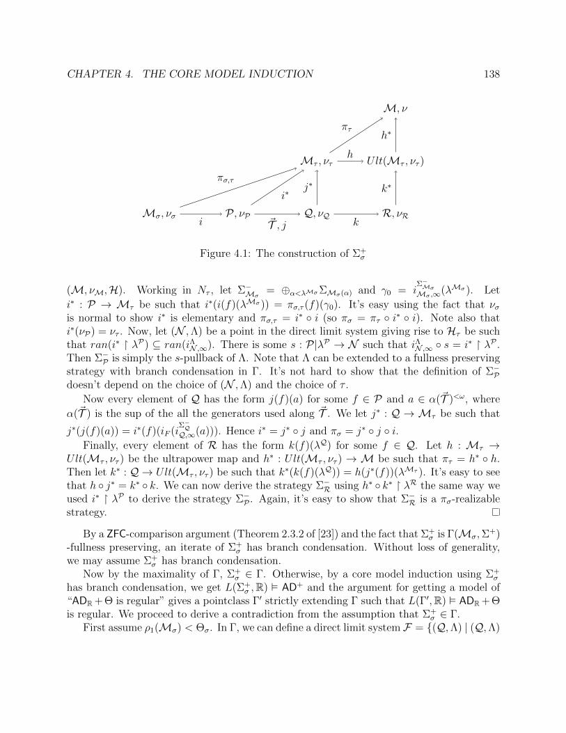
CHAPTER 4. THE CORE MODEL INDUCTION 138
Mσ, νσ P , νP Q, νQ R, νR
Mτ , ντ Ult(Mτ , ντ )
M, ν
i ~T , j k
πσ,τ
i∗
h
j∗
πτh∗
k∗
Figure 4.1: The construction of Σ+σ
(M, νM,H). Working in Nτ , let Σ−Mσ= ⊕α<λMσΣMσ(α) and γ0 = i
Σ−MσMσ ,∞(λMσ). Let
i∗ : P → Mτ be such that i∗(i(f)(λMσ)) = πσ,τ (f)(γ0). It’s easy using the fact that νσis normal to show i∗ is elementary and πσ,τ = i∗ i (so πσ = πτ i∗ i). Note also thati∗(νP) = ντ . Now, let (N ,Λ) be a point in the direct limit system giving rise to Hτ be suchthat ran(i∗ λP) ⊆ ran(iΛN ,∞). There is some s : P|λP → N such that iΛN ,∞ s = i∗ λP .Then Σ−P is simply the s-pullback of Λ. Note that Λ can be extended to a fullness preservingstrategy with branch condensation in Γ. It’s not hard to show that the definition of Σ−Pdoesn’t depend on the choice of (N ,Λ) and the choice of τ .
Now every element of Q has the form j(f)(a) for some f ∈ P and a ∈ α(~T )<ω, where
α(~T ) is the sup of the all the generators used along ~T . We let j∗ : Q → Mτ be such that
j∗(j(f)(a)) = i∗(f)(iF (iΣ−QQ,∞(a))). Hence i∗ = j∗ j and πσ = j∗ j i.
Finally, every element of R has the form k(f)(λQ) for some f ∈ Q. Let h : Mτ →Ult(Mτ , ντ ) be the ultrapower map and h∗ : Ult(Mτ , ντ ) → M be such that πτ = h∗ h.Then let k∗ : Q → Ult(Mτ , ντ ) be such that k∗(k(f)(λQ)) = h(j∗(f))(λMτ ). It’s easy to seethat h j∗ = k∗ k. We can now derive the strategy Σ−R using h∗ k∗ λR the same way weused i∗ λP to derive the strategy Σ−P . Again, it’s easy to show that Σ−R is a πσ-realizablestrategy.
By a ZFC-comparison argument (Theorem 2.3.2 of [23]) and the fact that Σ+σ is Γ(Mσ,Σ
+)-fullness preserving, an iterate of Σ+
σ has branch condensation. Without loss of generality,we may assume Σ+
σ has branch condensation.Now by the maximality of Γ, Σ+
σ ∈ Γ. Otherwise, by a core model induction using Σ+σ
has branch condensation, we get L(Σ+σ ,R) AD+ and the argument for getting a model of
“ADR+ Θ is regular” gives a pointclass Γ′ strictly extending Γ such that L(Γ′,R) ADR+ Θis regular. We proceed to derive a contradiction from the assumption that Σ+
σ ∈ Γ.First assume ρ1(Mσ) < Θσ. In Γ, we can define a direct limit system F = (Q,Λ) | (Q,Λ)
CHAPTER 4. THE CORE MODEL INDUCTION 139
≡ (Mσ,Σ+σ )32 (this uses that Σ+
σ ∈ Γ). Let M∞ be the direct limit of F . HenceM∞ ∈ HODΓ, HODΓ|γσ M∞ by fullness preservation of Σσ, and ρ1(M∞) < γσ. Thismeans M∞ constructs a bounded subset of γσ in HODΓ but not in HODΓ|γσ. This contra-dicts the fact that HODΓ|γσ = V HODΓ
γσ and γσ is a strong limit cardinal in HODΓ.Now assume ρ1(Mσ) = Θσ and let A ⊆ Θσ be a set Σ1 definable over Mσ but not in
LpΣσ(Hσ) (A exists by our assumption). Say
α ∈ A⇔Mσ ψ[α, s, pMσ1 ], (4.12)
for some s ∈ Θ<ωσ . Recall that Mσ Θσ is measurable as witnessed by νσ. We define F
as above33. Let M∞ be the direct limit of F and let iMσ ,∞ : Mσ → M∞ be the iterationembedding. We have that HODΓ|γσ M∞ ∈ HODΓ and ρ1(M∞) = γσ. Let A∞ be definedover M∞ the same way A is defined over Mσ, i.e.
α ∈ A∞ ⇔M∞ ψ[α, iMσ ,∞(s), pM∞1 ]. (4.13)
Since A∞ is ODΓ, A is ordinal definable from (Hσ,Σσ) in Γ. By mouse capturing in Γ,A ∈ LpΣσ(Hσ). Contradiction.
Lemma 4.3.33. Suppose Γ = L(Γ,R)∩Γ. Then L[H+, ν](Γ)∩P(R) = Γ and L[H+, ν](Γ) ADR+ there is an R-complete measure on Θ.
Proof. The equality of in the conclusion of the lemma follows from Theorem 4.3.19 withHODΓ playing the role of H and (H++, ν) playing the role of H+. Hence we also get(H++, ν)(Γ) ADR. The R-complete measure on Θ in (H++, ν)(Γ) comes from ν from theproof of Theorem 2.4 in [3]. The proof uses the fact that every A ∈ Γ can be added to(H++, ν) via a forcing of size < Θ.
This completes the proof of Theorem 4.3.16.
32This means these hod pairs are Dodd-Jensen equivalent. The fine structural details involved in thecomparison process is described in [23].
33We take Σ0-ultrapowers for extenders with critical points ≥ the image of Θσ under iteration embeddingsby Σσ and Σ1-ultrapowers otherwise
140
Index
<w, 7B-iterability, 68B(P ,Σ), 6D(M,λ), 58D+(M,λ), 58FJ(M), 9F ∗J (a), 11HP,ΣB , 68HP,ΣB,m, 68H(P, ~f), 87Hom∗, 57, 114Hom∞, 114I(P ,Σ), 6J-mouse, 12J-premouse, 12JΓ
Σ,A, 96KΣ(R), 56LpΓ,Σ(a), 6Xα, 14Γ-MC(Σ), 98Γ-fullness preservation, 6Γ-hod pair construction, 7Γ(P ,Σ), 7Γub, 114M+, 96P−, 68Σ-iterable, 56Σ-mouse, 6Σ2
1 degree, 25T ϕM , 11TM , 11Θ, 3γP,ΣB , 68
γP,ΣB,m, 68
γQ,0Di,m, 74
γQ,0Di, 74
γ(P, ~f), 87∞-Borel code, 3B(P−,Σ), 68Dα, 25Rf , 14F , 69θA, 3Ehod, 5fβ, 14k-suitable premouse, 58l(M), 9n-suitable Σ-premouse, 67AD+, 1, 3
Branch condensation, 107
club, clα,F , 17core model induction operators, 97
determines itself on generic extensions, 10
fineness, 14fullness preservation, 6
good pointclass, 4good Woodin cardinal, 114
hod initial segment, 5hod mice, 1hod pair, 5hod premouse, 5HPΓ, 7
INDEX 141
inductive-like pointclass, 4
MiceΓ, 7model operator, 8Mouse Set Conjecture, 2
new derived model, 58nice, 14normality, 14
old derived model, 58
plain Σ-mouse operator, 96potential J-premouse, 12
Quasi-iterability conjecture, 98
scub, 133seal a gap, 97self-justifying-system, sjs, 62strong B-condensation, 69strong B-iterability, 69strong club, 133Strong Mouse Capturing, SMC, 7Strong Mouse Set Conjecture, SMSC, 7super γ-fullness preserving, 6Suslin capturing, 4swo, 97
tail filter, 18term relation hybrid mouse operator, 96
ultra-homogenous ideal, 43universally Baire sets, 114
Wadge rank, 3wcub, 133weak club, 133weakly coherent extender sequence, 15
142
Bibliography
[1] H. Becker. AD and the supercompactness of ℵ1. Journal of Symbolic Logic, pages 822–842,1981.
[2] A. Blass. Equivalence of two strong forms of determinacy. Proceedings of the AmericanMathematical Society, 52:373–376, 1975.
[3] A.E Caicedo, P. Larson, G. Sargsyan, R.D. Schindler, J.R. Steel, and M. Zeman. Squareprinciples in Pmax extesions. arXiv preprint arXiv:1205.4275, 2012.
[4] J. Cummings. Iterated forcing and elementary embeddings. Handbook of set theory, pages775–883, 2010.
[5] D.A. Dubose. The equivalence of determinacy and iterated sharps. Journal of Symbolic Logic,pages 502–525, 1990.
[6] M. Gitik. Prikry-type forcings. Handbook of set theory, pages 1351–1447, 2010.
[7] L. Harrington. Analytic determinacy and 0]. The Journal of Symbolic Logic, 43:685–693, 1978.
[8] S. Jackson. Structural consequences of AD. Handbook of Set Theory, pages 1753–1876, 2010.
[9] Thomas Jech. Set theory. Springer Monographs in Mathematics. Springer-Verlag, Berlin, 2003.The third millennium edition, revised and expanded.
[10] A.S. Kechris and W.H. Woodin. Equivalence of partition properties and determinacy. Pro-ceedings of the National Academy of Sciences, 80(6):1783–1786, 1983.
[11] R. Ketchersid. Toward ADR from the Continuum Hypothesis and an ω1-dense ideal. PhDthesis, Ph. D. thesis, Berkeley, 2000.
[12] Richard Ketchersid. More structural consequences of AD. Contemporary Mathematics, 533:71–105, 2011.
[13] P. Koellner and W.H. Woodin. Large cardinals from determinacy. Handbook of Set Theory,pages 1951–2119, 2010.
[14] P.B. Larson. The stationary tower, volume 32 of University Lecture Series. American Mathe-matical Society, Providence, RI, 2004. Notes on a course by W. Hugh Woodin.
BIBLIOGRAPHY 143
[15] P.B. Larson. Forcing over models of determinacy. Handbook of Set Theory, pages 2121–2177,2010.
[16] D.A. Martin and J.R. Steel. The extent of scales in L(R), cabal seminar 79–81. Lecture Notesin Math, 1019:86–96.
[17] W. J. Mitchell and J. R. Steel. Fine structure and iteration trees, volume 3 of Lecture Notesin Logic. Springer-Verlag, Berlin, 1994.
[18] I. Neeman. Games of countable length. LONDON MATHEMATICAL SOCIETY LECTURENOTE SERIES, pages 159–196, 1999.
[19] I. Neeman. The determinacy of long games, volume 7. De Gruyter, 2004.
[20] G. Sargsyan. On the strength of PFA I.
[21] G. Sargsyan. A tale of hybrid mice. PhD thesis, Berkeley, 2009.
[22] G. Sargsyan and N. Trang. Non-tame mice from tame failures of the unique branch hypothesis.arXiv preprint arXiv:1211.0761, 2012.
[23] Grigor Sargsyan. A tale of hybrid mice, available at http://math.rutgers.edu/ gs481/msc.pdf.
[24] E. Schimmerling and J. R. Steel. The maximality of the core model. Trans. Amer. Math. Soc.,351(8):3119–3141, 1999.
[25] R. Schindler. Woodin’s axiom (*), bounded forcing axioms, and precipitous ideals on ω1,available at http://wwwmath.uni-muenster.de/u/rds/star.pdf.
[26] R. Schindler and J. R. Steel. The core model induction. Available at math.berkeley.edu/∼steel.
[27] F. Schlutzenberg and N. Trang. Scales in LpΣ(R), in preparation.
[28] R. Solovay. The independence of DC from AD. In Cabal Seminar 76–77, pages 171–183.Springer, 1978.
[29] J. R. Steel. The derived model theorem, available at www.math.berkeley.edu/∼ steel.
[30] J. R. Steel. A theorem of Woodin on mouse sets, available athttp://math.berkeley.edu/∼steel/.
[31] J. R. Steel. Woodin’s analysis of HODL(R), available at www.math.berkeley.edu/∼ steel.
[32] J. R. Steel. Closure properties of pointclasses. In Cabal Seminar 77–79, pages 147–163.Springer, 1981.
[33] J. R. Steel. The core model iterability problem, volume 8 of Lecture Notes in Logic. Springer-Verlag, Berlin, 1996.
[34] J. R. Steel. PFA implies ADL(R). J. Symbolic Logic, 70(4):1255–1296, 2005.
BIBLIOGRAPHY 144
[35] J. R. Steel. Derived models associated to mice. In Computational prospects of infinity. Part I.Tutorials, volume 14 of Lect. Notes Ser. Inst. Math. Sci. Natl. Univ. Singap., pages 105–193.World Sci. Publ., Hackensack, NJ, 2008.
[36] J. R. Steel. An optimal consistency strength lower bound for ADR. Unpublished notes, 2008.
[37] J. R. Steel. Scales in K(R). In Games, scales, and Suslin cardinals. The Cabal Seminar. Vol.I, volume 31 of Lect. Notes Log., pages 176–208. Assoc. Symbol. Logic, Chicago, IL, 2008.
[38] J. R. Steel. Scales in K(R) at the end of a weak gap. J. Symbolic Logic, 73(2):369–390, 2008.
[39] J. R. Steel. Scales in K(R) at the end of a weak gap. J. Symbolic Logic, 73(2):369–390, 2008.
[40] J. R. Steel and N. Trang. AD+, derived models, and Σ1-reflection, available athttp://math.berkeley.edu/∼namtrang.
[41] J. R. Steel and W. H. Woodin. HOD as a core model. In Ordinal definability and recursiontheory: Cabal Seminar, Vol. III. 2012.
[42] J.R. Steel. An outline of inner model theory. Handbook of set theory, pages 1595–1684, 2010.
[43] N. Trang. HOD in natural models of AD+. arXiv preprint arXiv:1201.6128, 2012.
[44] N. Trang. Structure theory of L(R, µ), in preparation. 2012.
[45] N. Trang and T. Wilson. Supercompact measures on Pω1(P(R)), in preparation. 2012.
[46] T. Wilson. Contributions to descriptive inner model theory. PhD thesis, Berkeley, 2012.
[47] W. H. Woodin. AD and the uniqueness of the supercompact measures on Pω1 (λ). In CabalSeminar 79–81, pages 67–71. Springer, 1983.
[48] W. H. Woodin. The axiom of determinacy, forcing axioms, and the nonstationary ideal,volume 1 of de Gruyter Series in Logic and its Applications. Walter de Gruyter & Co., Berlin,1999.


![RE VERA INSTITUTE OF THECHNOLOGY MANDATORY … · 1 Mr.Pravin Shinde HOD [COM] 2 Mr.Anuj Batham HOD[MECH] 3 Mrs.Bijeta Das HOD[CIVIL] 4 Mr.Nilesh Patil HOD[EXTC] 5 Mrs.Yogita Wasu](https://img.pdfslide.us/doc/110x75/5f6ce3d422557a4c93388866/re-vera-institute-of-thechnology-mandatory-1-mrpravin-shinde-hod-com-2-mranuj.jpg)