1

Generalized Score DistributionLucjan Janowski, Bogdan Cmiel, Krzysztof Rusek, Jakub Nawała, Zhi Li

Abstract—A class of discrete probability distributions containsdistributions with limited support, i.e. possible argument valuesare limited to a set of numbers (typically consecutive). Examplesof such data are results from subjective experiments utilizingthe Absolute Category Rating (ACR) technique, where possibleanswers (argument values) are 1, 2, · · · , 5 or typical Likertscale −3,−2, · · · , 3. An interesting subclass of those distri-butions are distributions limited to two parameters: describingthe mean value and the spread of the answers, and having nomore than one change in the probability monotonicity. In thispaper we propose a general distribution passing those limitationscalled Generalized Score Distribution (GSD). The proposed GSDcovers all spreads of the answers, from very small, given bythe Bernoulli distribution, to the maximum given by a BetaBinomial distribution. We also show that GSD correctly describessubjective experiments scores from video quality evaluationswith probability of 99.7%. A Google Collaboratory websitewith implementation of the GSD estimation, simulation, andvisualization is provided.

Index Terms—Quality of Experience, Subject model, Subjectiveexperiment, Data analysis, New distribution

I. INTRODUCTION

SUBJECTIVE experiments let us collect users’ opinionsabout a specific system. Such experiment can be seen as

a measuring device. Any measuring device provides certainprecision. In this article we analyze subjects’/testers’/users’answers, in order to better understand the random processgenerating those answers. The obtained result is general andcovers interesting class of discrete distributions with limitedsupport, and two parameters describing the mean and theanswer’s spread.

Our main goal is to check what is the distribution ofanswers provided by subjects. We limit our considerations topopular subjective experiments using discrete five point scale1, 2, · · · , 5. For this scale, numerous different databases areavailable therefore we compare the theoretical and analyticalresults. Nevertheless, the proposed model is general and in theAppendix B we describe the generalization to M point scale.

Knowing the answers’ distribution provides important in-formation about the answering process. Further modeling ofthis process can lead to better understanding of experimentsinvolving subjects [1]. The ultimate goal is to make data anal-ysis of those experiments more precise. Better understandingwhich factors influence the obtained answer allows to remove,or compensate, those aspects in the data analysis.

The main contribution of this paper is to propose a newGeneralized Score Distribution (GSD), and provide a strong

B. Cmiel is with the Department of Applied Mathematics, AGH Universityof Science and Technology, Poland.

L. Janowski, J. Nawała, and K. Rusek are with the Department of Telecom-munictions of AGH University of Science and Technology, Poland. e-mail:janowski@kt.agh.edu.pl

Z. Li is with Netflix

evidence that GSD describes the answering process in a videoquality test correctly. We strongly believe that GSD distribu-tion can be useful in different fields of science, since it is ageneralization of the existing and widely used distributions.For the proposed distribution the estimation algorithm1 isprovided and analyzed by extensive simulation study. Theanalysis of different existing video quality databases allow usto estimate typical parameters of this model. Those results canbe used as a prior distribution of the GSD parameters in thefuture analysis such as Bayes estimator.

In order to validate GSD in the context of subjectiveexperiments we have used four different databases, with morethan 1,800 PVSs (Processed Video Sequences, i.e. scoredsequences). The analyzed PVSs have different number of votesfrom typical 24 up to 213. The final score shows that GSDdescribes the answers correctly with probability of 99.7%.

In the next section we describe the related work. Section IIIdescribes the proposed distribution with the estimation processdetailed in Section IV. Section V provides short descriptionsof the data sets used. Section VI presents the results. The lastsection concludes the paper.

II. RELATED WORK

Subject answers analysis is a broad topic considered in nu-merous publications starting from ITU standards to technicalpublications provided by companies. The standard focusing onthe objective metrics evaluation is ITU-T P.1401 [2]. Its maingoal is to describe correct way of analyzing subjective data.Similarly, a recent publication [3] describes the problem ofcorrect way of comparing groups within subjective experiment.

Beyond correctness in the literature we can find interestingproposals for other than typical, focused on MOS, analysis.In [4] a number of different metrics related to user behaviorand service acceptance are described. In [5] a method to findeach answer probability is suggested. More recently similarapproach to model each answer probability, instead of simplemean (MOS), was proposed in [6]. Other publications arefocused on modeling Quality of Experience in general e.g.[7]. The model we propose in this paper is in line with thoseanalysis as the model is discrete.

Not many publications focus on the answering process,especially the precision of the obtained score. An interestinganalysis is shown in [8], where the relation between MOSand the standard deviation of scores is studied. In the papera unique parameter HSE2, describing the test difficulty was

1The implementation can be found here https://colab.research.google.com/drive/1ioM4JqUaEA8fHJH9V-0iphHt4C9zmI0i

2In the original paper the parameter was named SOS but we think that HSE(from Hossfeld, Schatz, and Egger) will be a better, unambiguous name. SOSis traditionally used to describe standard deviation of scores.

arX

iv:1

909.

0436

9v1

[st

at.M

E]

10

Sep

2019

2

proposed. Another interesting proposal analyzing the subjec-tive experiment precision is [9] where different confidenceintervals are studied.

The analysis of the subjective experiment leads to proposingtwo subject models in [10] and [11]. Those models arediscussed in more detail further in the paper. User modelallows to extend analysis of the subjective experiments likethe one described in [1], [12], or make the existing analysismore precise [13], [14]. The user model is modified in [15],[16], [17] which leads to new results, e.g. showing that thecontent has significant influence on both variability and meanof the obtained answers [17].

The new subject model proposed in this paper extendsthe existing analysis by introducing discrete distribution. Theprevious publications used continuous process with discretiza-tion and censoring (clipping). As the next section describes,this introduces certain error. Therefore, the proposed discretemodel, not having this error, is a better solution.

In this paper we do not compare our model to modelsused in different fields working on quality. It is left as aninteresting future research. Comparing to those modes isdifficult, since all those models need a different data, whichdo not exists commonly in the video quality community. Anexample could be food industry using “Panel Check” [18],[19], the method proposed by Pane Check relay strongly onthe lack of tied answers. For the five point scale used in videoquality evaluation, small number of tied answers is a strongassumption.

In psychology the signal detection theory (SDT) is usedin the context of subjective quality scores analysis [20], [21].Such analysis can be complicated taking into account differentinfluencing factors [22]. This is especially an interestingconnection between QoE and psychology, nevertheless, againa slightly different data are needed. To use SDT we need arecognition and a quality score, in the video quality analysiscase only quality scores are available.

It is also worth mentioning that the distribution proposed inthis paper can be used for modeling an answering in Likertscale surveys. For example, in [23] the authors consider theimpact of the number of response categories on the reliabilityof the measurements. In the model of answers provided inequation (1) of [23] one can consider GSD distribution of therandom error to estimate the latent unobserved true score. Thesame approach can also be used for example in [24] wherethe problem of measuring patients experience in hospitals isconsidered.

III. SUBJECT ANSWERS AS A RANDOM VARIABLE

Assuming that a test is conducted using five point discretescale the subject answer U has a multinomial distribution givenby:

P (U = s) = ps, where5∑s=1

ps = 1 (1)

Such description of a subject answers distribution is generalbut has four different parameters, coming from five probabil-ities.

In general we can describe the subject answer as a function:

U = ψ + ε, (2)

where ψ is the true quality and ε is an error term. Analgorithm predicting quality should aim in estimating ψ. Still,the error distribution is important and should be modeled. Theerror term represents precision of ψ estimation. Note that thevariance term (represented by ε) cannot be too complicated.In total, we have four different probabilities. Therefore, wewould like to use a model for which the variance is describedby a single parameter. We can then use it to predict the truequality. In turn, accuracy of its estimation is denoted by thevariance parameter.

For simplicity, we only consider a single sequence (i.e.,PVS) analysis. In general, we consider a model, where ananswer for a sequence is a random variable U drawn from adistribution:

U ∼ F (ψ, θ), (3)

where ψ is the true quality, θ is a parameter describing answersspread, and F () a cumulative distribution function. However,in the text we mark θ differently, depending on the model weare considering. This notation makes the description clearer.

Our notation convention generally follows guidelines ofSAM (Statistical Analysis Methods) of VQEG (Video QualityExpert Group) group, described in [25]. Nevertheless, weintroduce extensions to selected symbols.

A. Continuous Model

The models proposed by [10] and [11] describe a subjectanswer as a continuous normal distribution with certain meanψ, which is true quality, and standard deviation σ describingthe error. Therefore, the subject answer is O ∼ N (ψ, σ).Since a subjective scale is discrete we cannot observe O. Toconvert a continuous answer to a discrete one, a subject makesdiscretization and censoring (clipping). This process convertscontinuous random variable O to discrete variable U . We cancalculate each answer probability (i.e., U distribution), as afunction of ψ and σ by the below equations:

P (U = s) =

∫ s+0.5

s−0.5

1

2πσe−

(x−ψ)2

2σ2 (4)

for s = 2, 3, 4 and

P (U = 1) =

∫ 1.5

−∞

1

2πσe−

(x−ψ)2

2σ2 (5)

P (U = 5) =

∫ ∞4.5

1

2πσe−

(x−ψ)2

2σ2 (6)

Note that the parameters estimated from O and U can resultin different ψ and σ values since the support of O is any realnumber and the support of U is set 1, 2, · · · , 5. Let us markby ψo and σo the parameters of O distribution which are ourinput parameters and by ψu and σu the mean and standarddeviation of random variable U . For a given input pair (ψo, σo)the comparison with the obtained (ψu, σu) is crucial, since weinterpret the input parameters but the real process will behaveaccording to the output parameters. For the ideal model those

3

1 2 3 4 5

1

2

3

4

5

ψo

ψu

ObtainedCorrect

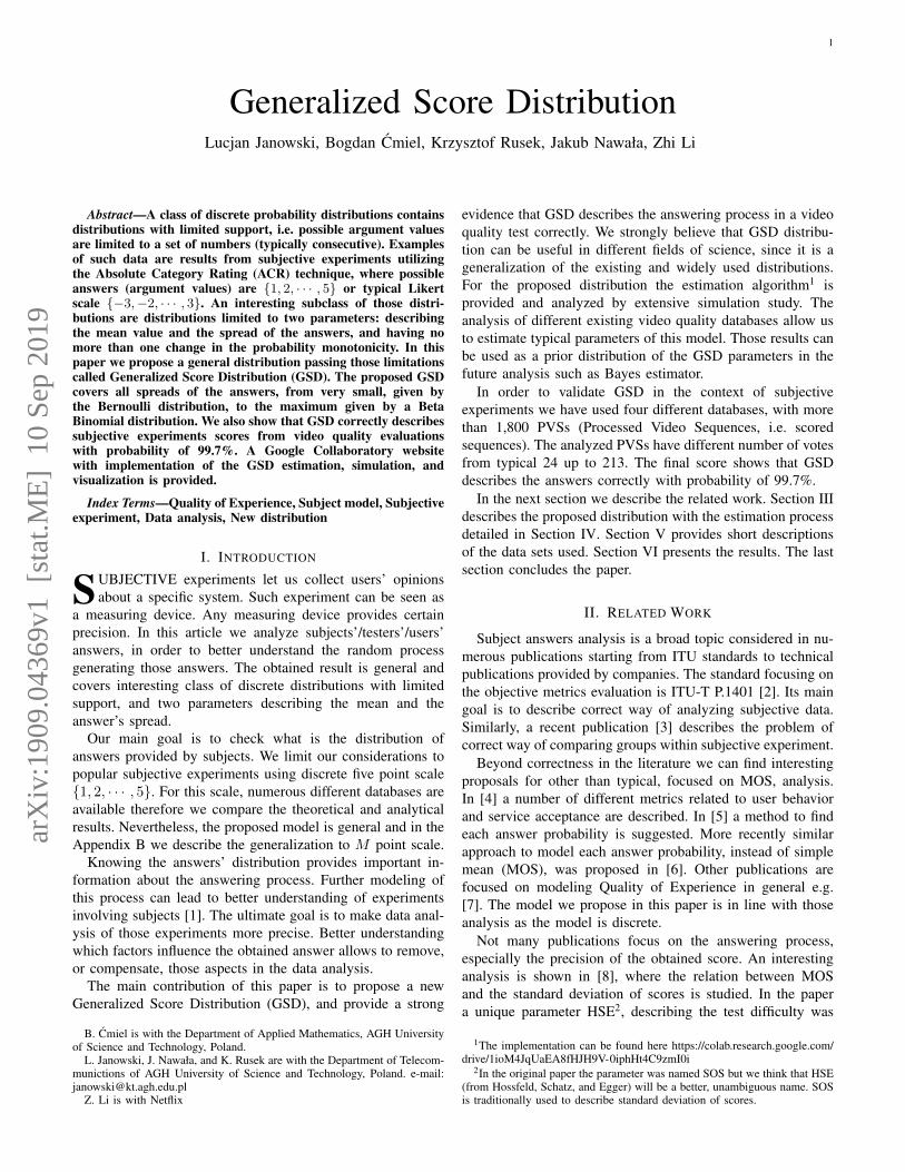
Fig. 1: The difference between ψo (the true quality for contin-uous model) and ψu (the true quality for discrete model) forσ = 0.1. The straight line represents an ideal model. The redline is the obtained value.

1 2 3 4 5

1

2

3

4

5

ψo

ψu

ObtainedCorrect

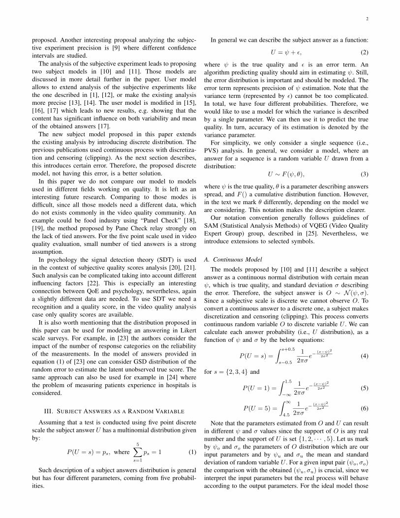
Fig. 2: The difference between ψo (the true quality for contin-uous model) and ψu (the true quality for discrete model) forσ = 1. The straight line represents an ideal model. The redline is the obtained value.

two values should be identical. In Fig. 1 and 2 we comparedthe relation between ψo and ψu for σo = 0.1 and σo = 1respectively.

Both Fig. 1 and 2 show large differences between ψo andψu. To understand this discrepancy we have to understandthe dissimilarities of a continuous and discrete process. Forcontinuous process the parameters can have any possible valueso ψo ∈ (−∞,∞) and σo ∈ [0,∞). On the other hand,ψu ∈ [1, 5] and the range of σu depends on ψu. This is verydifferent from the continuous model, where those parametersare independent. This dependency is caused by a finite numberof arguments values (i.e., subject answers) of the discretedistributions. For example, if ψ = 1.1 the two most extreme,

1 2 3 4 5

ψ

0

1

2

3

4

V(U

)

Discrete

Continuous

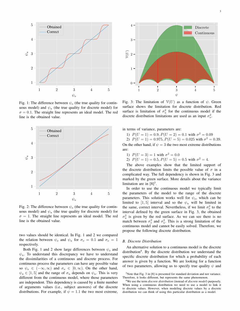
Fig. 3: The limitation of V(U) as a function of ψ. Greensurface shows the limitation for discrete distribution. Redsurface is limitation of σ2

u for the continuous model if thediscrete distribution limitations are used as an input σ2

o .

in terms of variance, parameters are:1) P (U = 1) = 0.9, P (U = 2) = 0.1 with σ2 = 0.092) P (U = 1) = 0.975, P (U = 5) = 0.025 with σ2 = 0.39.

On the other hand, if ψ = 3 the two most extreme distributionsare:

1) P (U = 3) = 1 with σ2 = 0.02) P (U = 1) = 0.5, P (U = 5) = 0.5 with σ2 = 4.The above examples show that the limited support of

the discrete distribution limits the possible value of σ in acomplicated way. The full dependency is shown in Fig. 3 andmarked by the green surface. More details about the variancelimitation are in [8]3.

In order to use the continuous model we typically limitthe parameters of the model to the range of the discreteparameters. This solution works well for ψo, which can belimited to [1, 5] interval and so the ψu will be limited inthe same, correct interval. Nevertheless, if we limit σ2

o to theinterval defined by the green surface in Fig. 3, the obtainedσ2u is given by the red surface. As we can see there is no

match between σ2o and σ2

u. This is a strong limitation of thecontinuous model and cannot be easily solved. Therefore, wepropose the following discrete distribution.

B. Discrete Distribution

An alternative solution to a continuous model is the discretedistribution4. By the discrete distribution we understand thespecific discrete distribution for which a probability of eachanswer is given by a function. We are looking for a functionof two parameters, allowing us to specify true quality ψ and

3Note that Fig. 3 in [8] is presented for standard deviation and not variance.Therefore, it looks different, but represents the same phenomenon.

4We use the term discrete distribution (instead of discrete model) purposely.When using a continuous distribution we need to use a model to link itto discrete values. However, when modeling discrete values by a discretedistribution we can think of using this particular distribution as a model.

4

the answers’ precision/spread σ. Since the discrete distributionparameter describing the distribution variance is not the sameas the process variance we mark it by ρ and not σ.

According to our knowledge there is no distribution de-scribed in literature which is:• discrete• supported on finite M element set• for any fixed mean covers the whole spectrum of possible

variances• with no more than a single change in the probabilities

monotonicity.Therefore, we propose a new distribution with two parametersdescribing mean ψ and variance ρ. The ρ parameter describesvariance for a given ψ. Since the proposed distribution isdiscrete the problems shown on Fig. 1 and 2 do not exist.

The proposed distribution utilizes existing discrete dis-tributions (with limited support), but covers more possiblevariances. An example of a discrete distribution which isdescribed by two parameters is Beta Binomial distribution[26]. Nevertheless, the smallest variance of the Beta Binomialdistribution is the Binomial distribution variance. It is a stronglimitation (in the case of subjective experiments for video)since in [9] it is suggested that the Binomial distribution hasthe highest possible variance for a correctly conducted subjec-tive experiment. Therefore, we need a different distribution.

1) GSD Definition: Let us start with the equation describingthe answers U for a particular PVS

U = ψ + ε, (7)

where ε is an error with mean value equals to 0. Since Ubelongs to the set 1, 2, ..., 5 then the distribution of ε hasto be supported on the set 1 − ψ, 2 − ψ, ..., 5 − ψ. Let usconsider shifted Binomial distribution for ε:

P (ε = k − ψ) =

(4

k − 1

)(ψ − 1

4

)k−1(5− ψ

4

)5−k

,

where k ∈ 1, ..., 5 is an user answer.Since the support of this distribution and the mean value are

fixed, we obtain fixed shifted Binomial distribution withoutany freedom. However, we would like to have a class ofdistributions for ε with all possible variances. Let us thinkabout how the set of all possible variances, for all distributionssupported on the set 1 − ψ, 2 − ψ, ..., 5 − ψ looks like.Remember that the mean values for such distributions are fixedto 0. This is why the set of all possible variances depends on ψ.If we denote by Vmin(ψ), Vmax(ψ) the minimal and maximalpossible variance respectively, then

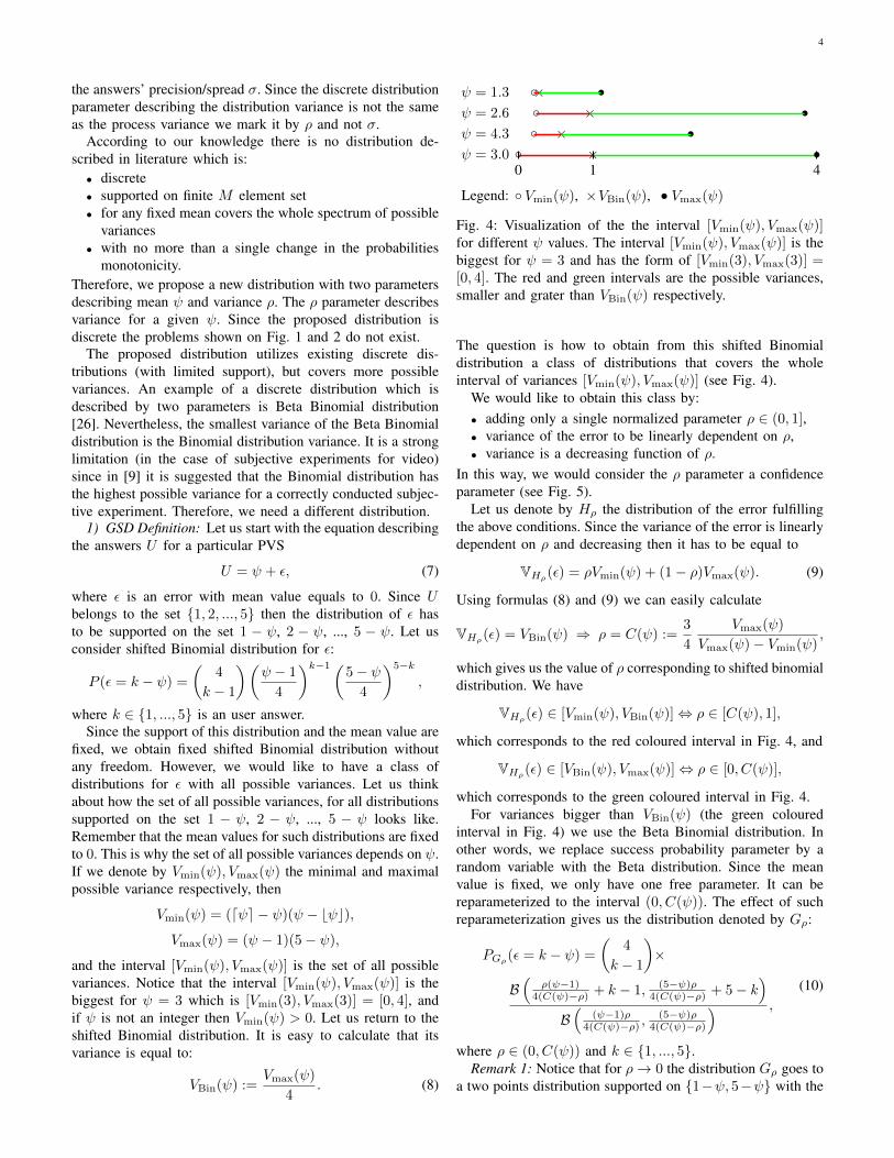
Vmin(ψ) = (dψe − ψ)(ψ − bψc),

Vmax(ψ) = (ψ − 1)(5− ψ),

and the interval [Vmin(ψ), Vmax(ψ)] is the set of all possiblevariances. Notice that the interval [Vmin(ψ), Vmax(ψ)] is thebiggest for ψ = 3 which is [Vmin(3), Vmax(3)] = [0, 4], andif ψ is not an integer then Vmin(ψ) > 0. Let us return to theshifted Binomial distribution. It is easy to calculate that itsvariance is equal to:

VBin(ψ) :=Vmax(ψ)

4. (8)

ψ = 1.3 × •ψ = 2.6 × •ψ = 4.3 × •ψ = 3.0 × •

0 1 4

Legend: Vmin(ψ), ×VBin(ψ), • Vmax(ψ)

Fig. 4: Visualization of the the interval [Vmin(ψ), Vmax(ψ)]for different ψ values. The interval [Vmin(ψ), Vmax(ψ)] is thebiggest for ψ = 3 and has the form of [Vmin(3), Vmax(3)] =[0, 4]. The red and green intervals are the possible variances,smaller and grater than VBin(ψ) respectively.

The question is how to obtain from this shifted Binomialdistribution a class of distributions that covers the wholeinterval of variances [Vmin(ψ), Vmax(ψ)] (see Fig. 4).

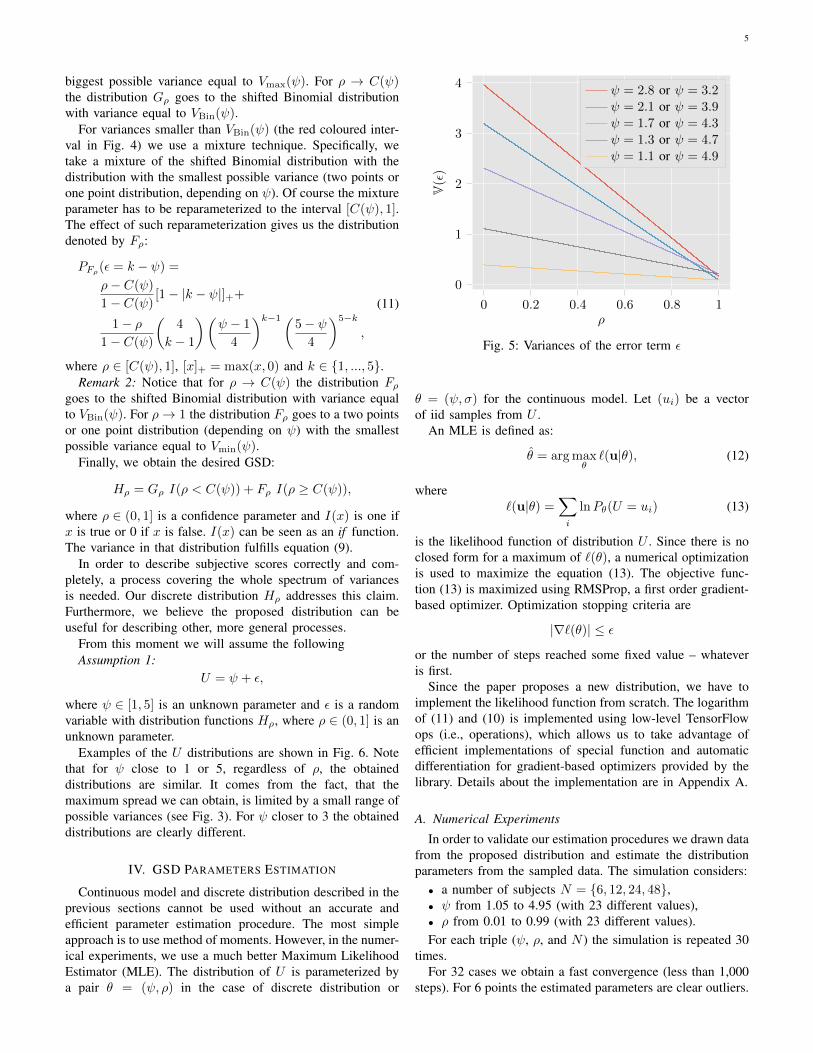
We would like to obtain this class by:• adding only a single normalized parameter ρ ∈ (0, 1],• variance of the error to be linearly dependent on ρ,• variance is a decreasing function of ρ.

In this way, we would consider the ρ parameter a confidenceparameter (see Fig. 5).

Let us denote by Hρ the distribution of the error fulfillingthe above conditions. Since the variance of the error is linearlydependent on ρ and decreasing then it has to be equal to

VHρ(ε) = ρVmin(ψ) + (1− ρ)Vmax(ψ). (9)

Using formulas (8) and (9) we can easily calculate

VHρ(ε) = VBin(ψ) ⇒ ρ = C(ψ) :=3

4

Vmax(ψ)

Vmax(ψ)− Vmin(ψ),

which gives us the value of ρ corresponding to shifted binomialdistribution. We have

VHρ(ε) ∈ [Vmin(ψ), VBin(ψ)]⇔ ρ ∈ [C(ψ), 1],

which corresponds to the red coloured interval in Fig. 4, and

VHρ(ε) ∈ [VBin(ψ), Vmax(ψ)]⇔ ρ ∈ [0, C(ψ)],

which corresponds to the green coloured interval in Fig. 4.For variances bigger than VBin(ψ) (the green coloured

interval in Fig. 4) we use the Beta Binomial distribution. Inother words, we replace success probability parameter by arandom variable with the Beta distribution. Since the meanvalue is fixed, we only have one free parameter. It can bereparameterized to the interval (0, C(ψ)). The effect of suchreparameterization gives us the distribution denoted by Gρ:

PGρ(ε = k − ψ) =

(4

k − 1

)×

B(

ρ(ψ−1)4(C(ψ)−ρ) + k − 1, (5−ψ)ρ

4(C(ψ)−ρ) + 5− k)

B(

(ψ−1)ρ4(C(ψ)−ρ) ,

(5−ψ)ρ4(C(ψ)−ρ)

) ,

(10)

where ρ ∈ (0, C(ψ)) and k ∈ 1, ..., 5.Remark 1: Notice that for ρ→ 0 the distribution Gρ goes to

a two points distribution supported on 1−ψ, 5−ψ with the

5

biggest possible variance equal to Vmax(ψ). For ρ → C(ψ)the distribution Gρ goes to the shifted Binomial distributionwith variance equal to VBin(ψ).

For variances smaller than VBin(ψ) (the red coloured inter-val in Fig. 4) we use a mixture technique. Specifically, wetake a mixture of the shifted Binomial distribution with thedistribution with the smallest possible variance (two points orone point distribution, depending on ψ). Of course the mixtureparameter has to be reparameterized to the interval [C(ψ), 1].The effect of such reparameterization gives us the distributiondenoted by Fρ:

PFρ(ε = k − ψ) =

ρ− C(ψ)

1− C(ψ)[1− |k − ψ|]++

1− ρ1− C(ψ)

(4

k − 1

)(ψ − 1

4

)k−1(5− ψ

4

)5−k

,

(11)

where ρ ∈ [C(ψ), 1], [x]+ = max(x, 0) and k ∈ 1, ..., 5.Remark 2: Notice that for ρ → C(ψ) the distribution Fρ

goes to the shifted Binomial distribution with variance equalto VBin(ψ). For ρ→ 1 the distribution Fρ goes to a two pointsor one point distribution (depending on ψ) with the smallestpossible variance equal to Vmin(ψ).

Finally, we obtain the desired GSD:

Hρ = Gρ I(ρ < C(ψ)) + Fρ I(ρ ≥ C(ψ)),

where ρ ∈ (0, 1] is a confidence parameter and I(x) is one ifx is true or 0 if x is false. I(x) can be seen as an if function.The variance in that distribution fulfills equation (9).

In order to describe subjective scores correctly and com-pletely, a process covering the whole spectrum of variancesis needed. Our discrete distribution Hρ addresses this claim.Furthermore, we believe the proposed distribution can beuseful for describing other, more general processes.

From this moment we will assume the followingAssumption 1:

U = ψ + ε,

where ψ ∈ [1, 5] is an unknown parameter and ε is a randomvariable with distribution functions Hρ, where ρ ∈ (0, 1] is anunknown parameter.

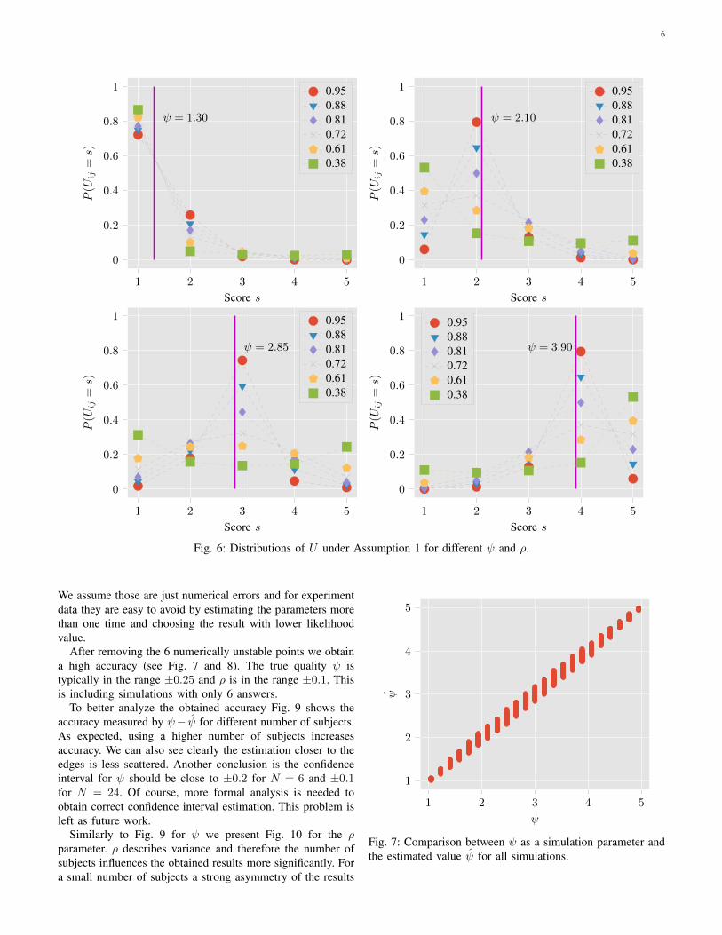
Examples of the U distributions are shown in Fig. 6. Notethat for ψ close to 1 or 5, regardless of ρ, the obtaineddistributions are similar. It comes from the fact, that themaximum spread we can obtain, is limited by a small range ofpossible variances (see Fig. 3). For ψ closer to 3 the obtaineddistributions are clearly different.

IV. GSD PARAMETERS ESTIMATION

Continuous model and discrete distribution described in theprevious sections cannot be used without an accurate andefficient parameter estimation procedure. The most simpleapproach is to use method of moments. However, in the numer-ical experiments, we use a much better Maximum LikelihoodEstimator (MLE). The distribution of U is parameterized bya pair θ = (ψ, ρ) in the case of discrete distribution or

0 0.2 0.4 0.6 0.8 1

0

1

2

3

4

ρ

V(ε

)

ψ = 2.8 or ψ = 3.2ψ = 2.1 or ψ = 3.9ψ = 1.7 or ψ = 4.3ψ = 1.3 or ψ = 4.7ψ = 1.1 or ψ = 4.9

Fig. 5: Variances of the error term ε

θ = (ψ, σ) for the continuous model. Let (ui) be a vectorof iid samples from U .

An MLE is defined as:

θ = arg maxθ`(u|θ), (12)

where`(u|θ) =

∑i

lnPθ(U = ui) (13)

is the likelihood function of distribution U . Since there is noclosed form for a maximum of `(θ), a numerical optimizationis used to maximize the equation (13). The objective func-tion (13) is maximized using RMSProp, a first order gradient-based optimizer. Optimization stopping criteria are

|∇`(θ)| ≤ ε

or the number of steps reached some fixed value – whateveris first.

Since the paper proposes a new distribution, we have toimplement the likelihood function from scratch. The logarithmof (11) and (10) is implemented using low-level TensorFlowops (i.e., operations), which allows us to take advantage ofefficient implementations of special function and automaticdifferentiation for gradient-based optimizers provided by thelibrary. Details about the implementation are in Appendix A.

A. Numerical Experiments

In order to validate our estimation procedures we drawn datafrom the proposed distribution and estimate the distributionparameters from the sampled data. The simulation considers:• a number of subjects N = 6, 12, 24, 48,• ψ from 1.05 to 4.95 (with 23 different values),• ρ from 0.01 to 0.99 (with 23 different values).For each triple (ψ, ρ, and N ) the simulation is repeated 30

times.For 32 cases we obtain a fast convergence (less than 1,000

steps). For 6 points the estimated parameters are clear outliers.

6

1 2 3 4 5

0

0.2

0.4

0.6

0.8

1

ψ = 1.30

Score s

P(U

ij=s)

0.950.880.810.720.610.38

1 2 3 4 5

0

0.2

0.4

0.6

0.8

1

ψ = 2.10

Score s

P(U

ij=s)

0.950.880.810.720.610.38

1 2 3 4 5

0

0.2

0.4

0.6

0.8

1

ψ = 2.85

Score s

P(U

ij=s)

0.950.880.810.720.610.38

1 2 3 4 5

0

0.2

0.4

0.6

0.8

1

ψ = 3.90

Score s

P(U

ij=s)

0.950.880.810.720.610.38

Fig. 6: Distributions of U under Assumption 1 for different ψ and ρ.

We assume those are just numerical errors and for experimentdata they are easy to avoid by estimating the parameters morethan one time and choosing the result with lower likelihoodvalue.

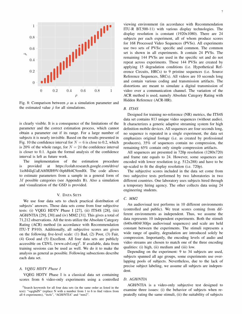
After removing the 6 numerically unstable points we obtaina high accuracy (see Fig. 7 and 8). The true quality ψ istypically in the range ±0.25 and ρ is in the range ±0.1. Thisis including simulations with only 6 answers.

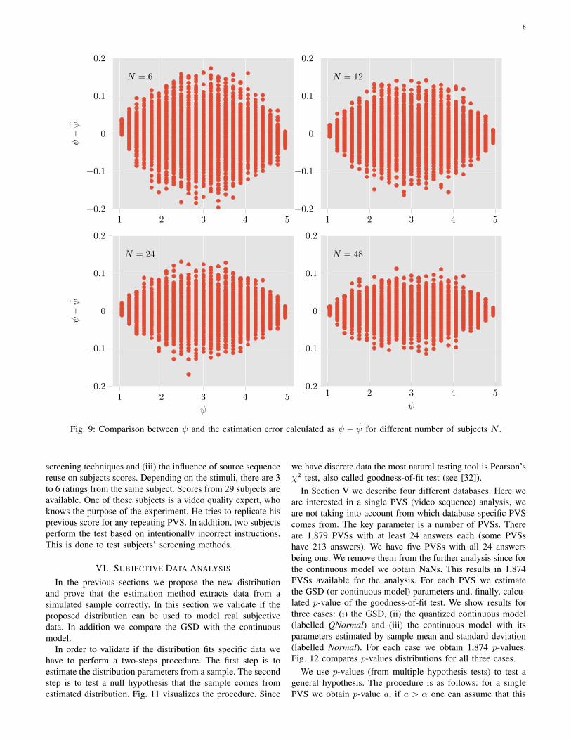
To better analyze the obtained accuracy Fig. 9 shows theaccuracy measured by ψ− ψ for different number of subjects.As expected, using a higher number of subjects increasesaccuracy. We can also see clearly the estimation closer to theedges is less scattered. Another conclusion is the confidenceinterval for ψ should be close to ±0.2 for N = 6 and ±0.1for N = 24. Of course, more formal analysis is needed toobtain correct confidence interval estimation. This problem isleft as future work.

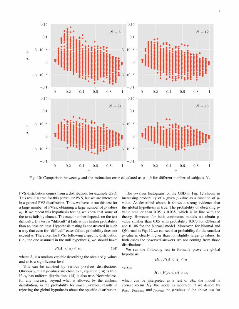
Similarly to Fig. 9 for ψ we present Fig. 10 for the ρparameter. ρ describes variance and therefore the number ofsubjects influences the obtained results more significantly. Fora small number of subjects a strong asymmetry of the results

1 2 3 4 5

1

2

3

4

5

ψ

ψ

Fig. 7: Comparison between ψ as a simulation parameter andthe estimated value ψ for all simulations.

7

0 0.2 0.4 0.6 0.8 1

0

0.2

0.4

0.6

0.8

1

ρ

ρ

Fig. 8: Comparison between ρ as a simulation parameter andthe estimated value ρ for all simulations.

is clearly visible. It is a consequence of the limitations of theparameter and the correct estimation process, which cannotobtain a parameter out if its range. For a large number ofsubjects it is nearly invisible. Based on the results presented inFig. 10 the confidence interval for N = 6 is close to 0.2, whichis 20% of the whole range, for N = 24 the confidence intervalis closer to 0.1. Again the formal analysis of the confidenceinterval is left as future work.

The implementation of the estimation procedureis provided at https://colab.research.google.com/drive/1ioM4JqUaEA8fHJH9V-0iphHt4C9zmI0i. The code allowsto estimate parameters from a sample in a general form ofM possible categories (see Appendix B). Also a simulationand visualization of the GSD is provided.

V. DATA SETS

We use four data sets to check practical distribution ofsubjects’ answers. Those data sets come from four subjectivetests: (i) VQEG HDTV Phase I [27], (ii) ITS4S [28], (iii)AGH/NTIA [29], [30] and (iv) MM2 [31]. This gives a total of71,212 observations. All the tests utilize the Absolute CategoryRating (ACR) method (in accordance with RecommendationITU-T P.910). Additionally, all subjective scores are givenon the following five-level scale: (1) Bad, (2) Poor, (3) Fair,(4) Good and (5) Excellent. All four data sets are publiclyaccessible on CDVL (www.cdvl.org)5. If available, data fromtraining sessions can be used as well. We do it to make theanalysis as general as possible. Following subsections describeeach data set.

A. VQEG HDTV Phase I

VQEG HDTV Phase I is a classical data set containingscores from 6 video-only experiments using a controlled

5Search keywords for all four data sets (in the same order as listed in thetext): “vqeghdN” (replace N with a number from 1 to 6 to find videos fromall 6 experiments), “its4s”, “AGH/NTIA” and “mm2”.

viewing environment (in accordance with RecommendationITU-R BT.500-11) with various display technologies. Thedisplay resolution is constant (1920x1080). There are 24subjects per each experiment, all of whom produce scoresfor 168 Processed Video Sequences (PVSs). All experimentsuse two sets of PVSs: specific and common. The commonset is shown in all experiments. It contain 24 PVSs. Theremaining 144 PVSs are used in the specific set and do notrepeat across experiments. Those 144 PVSs are created byapplying 15 degradation conditions (i.e. Hypothetical Ref-erence Circuits, HRCs) to 9 pristine sequences (i.e. SourceReference Sequences, SRCs). All videos are 10 seconds longand contain various coding and transmission artifacts. Thedistortions are meant to simulate a digital transmission ofvideo over a communication channel. The variation of theACR method is used, namely Absolute Category Rating withHidden Reference (ACR-HR).

B. ITS4SDesigned for training no-reference (NR) metrics, the ITS4S

data set contains 813 unique video sequences (without audio).It characterizes a generic adaptive streaming system for highdefinition mobile devices. All sequences are four seconds long,no sequence is repeated in a single experiment, the data setemphasizes original footage (i.e. as created by professionalproducers), 35% of sequences contain no compression, theremaining 65% contain only simple compression artifacts.

All sequences are presented in 720p resolution (1280x720)and frame rate equals to 24. However, some sequences areencoded with lower resolution (e.g. 512x288) and have to beup-scaled to fit the display resolution (i.e. 720p).

The subjective scores included in the data set come fromtwo subjective tests performed by two laboratories in twodifferent countries. One laboratory uses subjects hired througha temporary hiring agency. The other collects data using 24engineering students.

C. MM2An audiovisual test performs in 10 different environments

(controlled and public). We treat scores coming from dif-ferent environments as independent. Thus, we assume thedata represents 10 independent experiments. Both the stimuli(640x480@30fps audiovisual sequences) and scale are heldconstant between the experiments. The stimuli represents awide range of quality, degradation are introduced solely becompression. Importantly, the encoding levels of audio andvideo streams are chosen to match one of the three encodingqualities: (i) high, (ii) medium and (iii) low.

Depending on the experiment: 9 to 34 subjects are used,subjects spanned all age groups, some experiments use over-lapping pools of subjects. Nevertheless, due to the lack ofprecise subject labeling, we assume all subjects are indepen-dent.

D. AGH/NTIAAGH/NTIA is a video-only subjective test designed to

examine three issues: (i) the behavior of subjects when re-peatedly rating the same stimuli, (ii) the suitability of subjects

8

1 2 3 4 5−0.2

−0.1

0

0.1

0.2

ψ−ψ

N = 6

1 2 3 4 5−0.2

−0.1

0

0.1

0.2

N = 12

1 2 3 4 5−0.2

−0.1

0

0.1

0.2

ψ

ψ−ψ

N = 24

1 2 3 4 5−0.2

−0.1

0

0.1

0.2

ψ

N = 48

Fig. 9: Comparison between ψ and the estimation error calculated as ψ − ψ for different number of subjects N .

screening techniques and (iii) the influence of source sequencereuse on subjects scores. Depending on the stimuli, there are 3to 6 ratings from the same subject. Scores from 29 subjects areavailable. One of those subjects is a video quality expert, whoknows the purpose of the experiment. He tries to replicate hisprevious score for any repeating PVS. In addition, two subjectsperform the test based on intentionally incorrect instructions.This is done to test subjects’ screening methods.

VI. SUBJECTIVE DATA ANALYSIS

In the previous sections we propose the new distributionand prove that the estimation method extracts data from asimulated sample correctly. In this section we validate if theproposed distribution can be used to model real subjectivedata. In addition we compare the GSD with the continuousmodel.

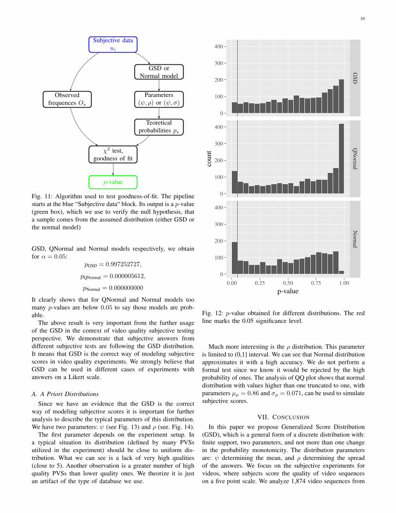
In order to validate if the distribution fits specific data wehave to perform a two-steps procedure. The first step is toestimate the distribution parameters from a sample. The secondstep is to test a null hypothesis that the sample comes fromestimated distribution. Fig. 11 visualizes the procedure. Since

we have discrete data the most natural testing tool is Pearson’sχ2 test, also called goodness-of-fit test (see [32]).

In Section V we describe four different databases. Here weare interested in a single PVS (video sequence) analysis, weare not taking into account from which database specific PVScomes from. The key parameter is a number of PVSs. Thereare 1,879 PVSs with at least 24 answers each (some PVSshave 213 answers). We have five PVSs with all 24 answersbeing one. We remove them from the further analysis since forthe continuous model we obtain NaNs. This results in 1,874PVSs available for the analysis. For each PVS we estimatethe GSD (or continuous model) parameters and, finally, calcu-lated p-value of the goodness-of-fit test. We show results forthree cases: (i) the GSD, (ii) the quantized continuous model(labelled QNormal) and (iii) the continuous model with itsparameters estimated by sample mean and standard deviation(labelled Normal). For each case we obtain 1,874 p-values.Fig. 12 compares p-values distributions for all three cases.

We use p-values (from multiple hypothesis tests) to test ageneral hypothesis. The procedure is as follows: for a singlePVS we obtain p-value a, if a > α one can assume that this

9

0 0.2 0.4 0.6 0.8 1−0.1

−5 · 10−2

0

5 · 10−2

0.1

0.15ρ−ρ

N = 6

0 0.2 0.4 0.6 0.8 1−0.1

−5 · 10−2

0

5 · 10−2

0.1

0.15

N = 12

0 0.2 0.4 0.6 0.8 1−0.1

−5 · 10−2

0

5 · 10−2

0.1

0.15

ρ

ρ−ρ

N = 24

0 0.2 0.4 0.6 0.8 1−0.1

−5 · 10−2

0

5 · 10−2

0.1

0.15

ρ

N = 48

Fig. 10: Comparison between ρ and the estimation error calculated as ρ− ρ for different number of subjects N .

PVS distribution comes from a distribution, for example GSD.This result is true for this particular PVS, but we are interestedin a general PVS distribution. Thus, we have to run this test fora large number of PVSs, obtaining a large number of p-valuesai. If we repeat this hypothesis testing we know that some ofthe tests fails by chance. The exact number depends on the testdifficulty. If a test is “difficult” it fails with a higher probabilitythan an “easier” test. Hypothesis testing is constructed in sucha way that even for “difficult” cases failure probability does notexceed α. Therefore, for PVSs following a specific distribution(i.e., the one assumed in the null hypothesis) we should have:

P (Ai < α) ≤ α, (14)

where Ai is a random variable describing the obtained p-valuesand α is a significance level.

This can be satisfied by various p-values distributions.Obviously, if all p-values are close to 1, equation (14) is true.If Ai has uniform distribution, (14) is also true. Nevertheless,for any increase, beyond what is allowed by the uniformdistribution, in the probability for small p-values, results inrejecting the global hypothesis about the specific distribution.

The p-values histogram for the GSD in Fig. 12 shows anincreasing probability of a given p-value as a function of p-value. As described above, it shows a strong evidence thatthe global hypothesis is true. The probability of observing p-value smaller than 0.05 is 0.035, which is in line with thetheory. However, for both continuous models we obtain p-value smaller than 0.05 with probability 0.073 for QNormaland 0.106 for the Normal model. Moreover, for Normal andQNormal in Fig. 12 we can see that probability for the smallestp-value is clearly higher than for slightly larger p-values. Inboth cases the observed answers are not coming from thosedistributions.

We run the following test to formally prove the globalhypothesis

H0 : P (A < α) ≤ α

versusH1 : P (A < α) > α,

which can be interpreted as a test of H0: the model iscorrect versus H1: the model is incorrect. If we denote bypGSD, pQNormal and pNormal the p-values of the above test for

10

Subjective dataui

GSD orNormal model

Parameters(ψ, ρ) or (ψ, σ)

Teoreticalprobabilities ps

Observedfrequences Os

χ2 test,goodness of fit

p-value

Fig. 11: Algorithm used to test goodness-of-fit. The pipelinestarts at the blue “Subjective data“ block. Its output is a p-value(green box), which we use to verify the null hypothesis, thata sample comes from the assumed distribution (either GSD orthe normal model)

GSD, QNormal and Normal models respectively, we obtainfor α = 0.05:

pGSD = 0.997252727,

pQNormal = 0.000005612,

pNormal = 0.000000000

It clearly shows that for QNormal and Normal models toomany p-values are below 0.05 to say those models are prob-able.

The above result is very important from the further usageof the GSD in the context of video quality subjective testingperspective. We demonstrate that subjective answers fromdifferent subjective tests are following the GSD distribution.It means that GSD is the correct way of modeling subjectivescores in video quality experiments. We strongly believe thatGSD can be used in different cases of experiments withanswers on a Likert scale.

A. A Priori Distributions

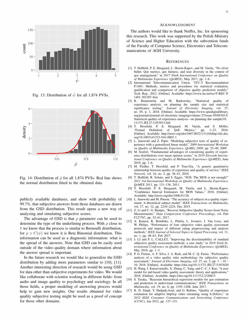
Since we have an evidence that the GSD is the correctway of modeling subjective scores it is important for furtheranalysis to describe the typical parameters of this distribution.We have two parameters: ψ (see Fig. 13) and ρ (see. Fig. 14).

The first parameter depends on the experiment setup. Ina typical situation its distribution (defined by many PVSsutilized in the experiment) should be close to uniform dis-tribution. What we can see is a lack of very high qualities(close to 5). Another observation is a greater number of highquality PVSs than lower quality ones. We theorize it is justan artifact of the type of database we use.

GSD

QN

ormal

Norm

al

0.00 0.25 0.50 0.75 1.00

0

100

200

300

400

0

100

200

300

400

0

100

200

300

400

p-value

coun

t

Fig. 12: p-value obtained for different distributions. The redline marks the 0.05 significance level.

Much more interesting is the ρ distribution. This parameteris limited to (0,1] interval. We can see that Normal distributionapproximates it with a high accuracy. We do not perform aformal test since we know it would be rejected by the highprobability of ones. The analysis of QQ plot shows that normaldistribution with values higher than one truncated to one, withparameters µρ = 0.86 and σρ = 0.071, can be used to simulatesubjective scores.

VII. CONCLUSION

In this paper we propose Generalized Score Distribution(GSD), which is a general form of a discrete distribution with:finite support, two parameters, and not more than one changein the probability monotonicity. The distribution parametersare: ψ determining the mean, and ρ determining the spreadof the answers. We focus on the subjective experiments forvideos, where subjects score the quality of video sequenceson a five point scale. We analyze 1,874 video sequences from

11

0

50

100

150

1 2 3 4 5ψ

coun

t

Fig. 13: Distribution of ψ for all 1,874 PVSs.

0

2

4

6

0.6 0.8 1.0ρ

dens

ity

Fig. 14: Distribution of ρ for all 1,874 PVSs. Red line showsthe normal distribution fitted to the obtained data.

publicly available databases, and show with probability of99.7%, that subjective answers from those databases are drawnfrom the GSD distribution. This result opens a new way ofanalyzing and simulating subjective scores.

The advantage of GSD is that ρ parameter can be used todetermine the type of the underlining process. With ρ close to1 we know that the process is similar to Bernoulli distribution,for ρ > C(ψ) we know it is Beta Binomial distribution. Thisinformation can be used as a diagnostic information: what isthe spread of the answers. Note that GSD can be easily usedoutside of the video quality domain where information aboutthe answer spread is important.

In the future research we would like to generalize the GSDdistribution by adding more parameters similar to [10], [11].Another interesting direction of research would be using GSDfor data other than subjective experiments for video. We wouldlike collaborate with scientist working in different fields: fromaudio and image quality to psychology and sociology. In allthose fields, a proper modeling of answering process wouldhelp to gain new insights. Our results obtained for videoquality subjective testing might be used as a proof of conceptfor those other domains.

ACKNOWLEDGMENT

The authors would like to thank Netflix, Inc. for sponsoringthis research. This work was supported by the Polish Ministryof Science and Higher Education with the subvention fundsof the Faculty of Computer Science, Electronics and Telecom-munications of AGH University.

REFERENCES

[1] T. Hoßfeld, P. E. Heegaard, L. Skorin-Kapov, and M. Varela, “No silverbullet: Qoe metrics, qoe fairness, and user diversity in the context ofqoe management,” in 2017 Ninth International Conference on Qualityof Multimedia Experience (QoMEX), May 2017, pp. 1–6.

[2] International Telecommunication Union, “ITU-T RecommendationP.1401: Methods, metrics and procedures for statistical evaluation,qualification and comparison of objective quality prediction models,”Tech. Rep., 2012. [Online]. Available: https://www.itu.int/rec/T-REC-P.1401-201207-I/en

[3] K. Brunnström and M. Barkowsky, “Statistical quality ofexperience analysis: on planning the sample size and statisticalsignificance testing,” Journal of Electronic Imaging, vol. 27,no. 05, p. 1, 2018. [Online]. Available: https://www.spiedigitallibrary.org/journals/journal-of-electronic-imaging/volume-27/issue-05/053013/Statistical-quality-of-experience-analysis--on-planning-the-sample/10.1117/1.JEI.27.5.053013.full

[4] T. Hossfeld, P. E. Heegaard, M. Varela, and S. Möller,“Formal Definition of QoE Metrics,” pp. 1–23, 2016.[Online]. Available: http://arxiv.org/abs/1607.00321%0Ahttp://dx.doi.org/10.1007/s41233-016-0002-1

[5] L. Janowski and Z. Papir, “Modeling subjective tests of quality of ex-perience with a generalized linear model,” 2009 International Workshopon Quality of Multimedia Experience, QoMEx 2009, pp. 35–40, 2009.

[6] M. Seufert, “Fundamental advantages of considering quality of experi-ence distributions over mean opinion scores,” in 2019 Eleventh Interna-tional Conference on Quality of Multimedia Experience (QoMEX), June2019, pp. 1–6.

[7] M. Fiedler, T. Hossfeld, and P. Tran-Gia, “A generic quantitativerelationship between quality of experience and quality of service,” IEEENetwork, vol. 24, no. 2, pp. 36–41, 2010.

[8] T. Hoßfeld, R. Schatz, and S. Egger, “SOS: The MOS is not enough!”2011 3rd International Workshop on Quality of Multimedia Experience,QoMEX 2011, pp. 131–136, 2011.

[9] T. Hossfeld, P. E. Heegaard, M. Varela, and L. Skorin-Kapov,“Confidence Interval Estimators for MOS Values,” 2018. [Online].Available: http://arxiv.org/abs/1806.01126

[10] L. Janowski and M. Pinson, “The accuracy of subjects in a quality exper-iment: A theoretical subject model,” IEEE Transactions on Multimedia,vol. 17, no. 12, pp. 2210–2224, Dec 2015.

[11] Z. Li and C. G. Bampis, “Recover Subjective Quality Scores from NoisyMeasurements,” Data Compression Conference Proceedings, vol. PartF127767, pp. 52–61, 2017.

[12] A. Kumcu, K. Bombeke, L. Platiša, L. Jovanov, J. Van Looy, andW. Philips, “Performance of four subjective video quality assessmentprotocols and impact of different rating preprocessing and analysismethods,” IEEE Journal of Selected Topics in Signal Processing, vol. 11,no. 1, pp. 48–63, Feb 2017.

[13] J. LI and P. L. CALLET, “Improving the discriminability of standardsubjective quality assessment methods: a case study,” in 2018 Tenth In-ternational Conference on Quality of Multimedia Experience (QoMEX),May 2018, pp. 1–3.

[14] P. G. Freitas, A. F. Silva, J. A. Redi, and M. C. Q. Farias, “Performanceanalysis of a video quality ruler methodology for subjective qualityassessment,” Journal of Electronic Imaging, vol. 27, no. 5, pp. 1 – 10 –10, 2018. [Online]. Available: https://doi.org/10.1117/1.JEI.27.5.053020

[15] H. Wang, I. Katsavounidis, X. Zhang, C. Yang, and C.-C. J. Kuo, “A usermodel for jnd-based video quality assessment: theory and applications,”2018. [Online]. Available: https://doi.org/10.1117/12.2320813

[16] S. Tasaka, “Bayesian hierarchical regression models for qoe estimationand prediction in audiovisual communications,” IEEE Transactions onMultimedia, vol. 19, no. 6, pp. 1195–1208, June 2017.

[17] K. D. Singh, Y. Hadjadj-Aoul, and G. Rubino, “Quality of experienceestimation for adaptive http/tcp video streaming using h.264/avc,” in2012 IEEE Consumer Communications and Networking Conference(CCNC), Jan 2012, pp. 127–131.

12

[18] R. Romano, P. B. Brockhoff, M. Hersleth, O. Tomic, and T. Næs,“Correcting for different use of the scale and the need for furtheranalysis of individual differences in sensory analysis,” Food Qualityand Preference, vol. 19, no. 2, pp. 197 – 209, 2008, 8th SensometricsMeeting.

[19] O. Tomic, A. Nilsen, M. Martens, and T. Næs, “Visualization of sensoryprofiling data for performance monitoring,” LWT - Food Science andTechnology, vol. 40, no. 2, pp. 262 – 269, 2007.

[20] B. Maniscalco and H. Lau, “A signal detection theoretic approachfor estimating metacognitive sensitivity from confidence ratings,” Con-sciousness and Cognition, vol. 21, pp. 422–430, 2012.

[21] S. Fleming and N. D. Daw, “Self-evaluation of decision-making: A gen-eral bayesian framework for metacognitive computation,” PsychologicalReview, vol. 124, pp. 91–114, 01 2017.

[22] J.-R. King and S. Dehaene, “A model of subjective report and objectivediscrimination as categorical decisions in a vast representational space,”Philosophical Transactions of The Royal Society B Biological Sciences,vol. 369, p. 20130204, 03 2014.

[23] D. F. Alwin, E. M. Baumgartner, and B. A. Beattie, “Number of responsecategories and reliability in attitude measurement,” Journal of SurveyStatistics and Methodology, vol. 6, pp. 212–239, 2018.

[24] D. L. Malott, B. R. Fulton, D. Rigamonti, and S. Myers, “Psychometrictesting of a measure of patient experience in Saudi Arabia and the UnitedArab Emirates,” Journal of Survey Statistics and Methodology, vol. 5,pp. 398–408, 2017.

[25] L. Janowski, J. Nawała, W. Robitza, Z. Li, L. Krasula, and K. Rusek,“Notation for subject answer analysis,” 2019.

[26] K. R. Coombes, The Beta-Binomial Distribution. [Online].Available: https://cran.r-project.org/web/packages/TailRank/vignettes/betabinomial.pdf

[27] M. Pinson, F. Speranza, M. Barkowski, V. Baroncini, R. Bitto, S. Borer,Y. Dhondt, R. Green, L. Janowski, T. Kawano et al., “Report on thevalidation of video quality models for high definition video content,”Video Quality Experts Group, 2010.

[28] M. H. Pinson, “Its4s: A video quality dataset with four-second unre-peated scenes,” NTIA/ITS, Tech. Rep. NTIA Technical Memo TM-18-532, Feb. 2018.

[29] L. Janowski and M. Pinson, “Subject bias: Introducing a theoretical usermodel,” in 2014 Sixth International Workshop on Quality of MultimediaExperience (QoMEX), Sep. 2014, pp. 251–256.

[30] M. H. Pinson and L. Janowski, “Agh/ntia: A video quality subjectivetest with repeated sequences,” NTIA/ITS, Tech. Rep. NTIA TechnicalMemo TM-14-505, June 2014.

[31] M. H. Pinson, L. Janowski, R. Pepion, Q. Huynh-Thu, C. Schmidmer,P. Corriveau, A. Younkin, P. Le Callet, M. Barkowsky, and W. Ingram,“The influence of subjects and environment on audiovisual subjectivetests: An international study,” IEEE Journal of Selected Topics in SignalProcessing, vol. 6, no. 6, pp. 640–651, Oct 2012.

[32] R. E. Walpole, R. H. Myers, S. L. Myers, and K. Ye, Probability &statistics for engineers and scientists, 8th ed. Upper Saddle River:Pearson Education, 2007.

APPENDIX AESTIMATION

Numerically optimized likelihood function

`(u|θ) =∑i

`B(ui|θ), ρ ≥ C(ψ)

`Bin(ui|θ) + f(ui, θ), ρ < C(ψ),

where

f(ui, θ) = log(1− ρ)− log(1− C(ψ))+

log(1 +(ρ− C(ψ))[1− |ui − ψ|]+(

4ui−1

) (ψ−14

)ui−1 (5−ψ4

)5−ui(1− ρ)

),

`B(ui|θ) is a logarithm of PGρ(ε = ui−ψ) given by (10) and`Bin is the likelihood function for Binomial distribution

`Bin(u, θ) = log

(4

u− 1

)+ (u−1)(log(ψ−1)− log(4))+

(5− u)(log(5− ψ)− log(4)).

Notice that the function f is the only place where we dothe computations in the probability domain (instead of logprobability), however it is build around log(1 + x) havingnumerically stable implementation in function log1p.

The logarithm of the newton symbol presents in both `Band `Bin can also be efficiently implemented as

log

(n

k

)= log Γ(n+1)−log Γ(k+1)−log Γ(n−k+1),

where log Γ is a logarithm of the gamma function, providedas a special function lgamma in TensorFlow. Notice that thiscomponent is commonly omitted from the likelihood becauseit does not depend on θ.

APPENDIX BGENERALIZATION

The described distribution is aiming 1, 2, · · · , 5scale/support. Here we present a generalization for1, 2, · · · ,M scale.

Let us denote

Vmin(ψ) = (dψe − ψ)(ψ − bψc),

Vmax(ψ) = (ψ − 1)(M − ψ),

C(ψ) =M − 2

M − 1

Vmax(ψ)

Vmax(ψ)− Vmin(ψ).

Let

PFρ(ε = k − ψ) =

ρ− C(ψ)

1− C(ψ)[1− |k − ψ|]+ +

1− ρ1− C(ψ)(

M − 1

k − 1

)(ψ − 1

M − 1

)k−1(M − ψM − 1

)M−k,

(15)

where ρ ∈ [C(ψ), 1], k = 1, ...,M and

PGρ(ε = k − ψ) =

(M − 1

k − 1

)B(

(ψ−1)ρ(M−1)(C(ψ)−ρ) + k − 1, (M−ψ)ρ

(M−1)(C(ψ)−ρ) +M − k)

B(

(ψ−1)ρ(M−1)(C(ψ)−ρ) ,

(M−ψ)ρ(M−1)(C(ψ)−ρ)

) ,

(16)

where ρ ∈ (0, C(ψ)), k = 1, ...,M .If we denote by Hρ the distribution function of the noise

then we assume that

Hρ = Gρ I(ρ < C(ψ)) + Fρ I(ρ ≥ C(ψ)),

where ρ ∈ (0, 1] is a confidence parameter (see Remark 3).Remark 3: The variance of the noise is equal to

VHρ(ε) = ρVmin(ψ) + (1− ρ)Vmax(ψ).

13

Since the variance of the noise is a decreasing function of ρ ∈(0, 1] then this parameter has an interpretation as a confidenceparameter.

From this moment we assume the followingAssumption 2:

U = ψ + ε,

where ψ ∈ [1,M ] is an unknown parameter, ε are independentrandom variables with distribution functions Hρ, where ρ ∈(0, 1] is an unknown parameter.