Generalized QBD Processes, Spectral Expansionand Performance Modeling Applications

Tien Van Do1 and Ram Chakka2

1 Department of TelecommunicationsBudapest University of Technology and Economics

H-1117, Magyar tudosok korutja 2., Budapest, Hungarydo@hit.bme.hu

2 Meerut Institute of Engineering and Technology (MIET),Meerut, India 250005.ramchakka@yahoo.com

Abstract. This paper suggests new queuing models, in the Markovianframework, which can tackle the presence of burstiness in the traffic andautocorrelations among the inter-arrival times of packets in the perfor-mance evaluation of next generation networks. These models are essen-tially based on certain generalizations of the Quasi Birth-Death (QBD)processes. Efficient steady state solution of these new queuing models,along with some illustrative applications, is presented. The proposedmodels and their further evolutions have the potential to be useful toolsfor the performance evaluation of modern telecommunication networks.

1 Introduction

The concept of Quasi Birth-Death (QBD) processes, as a generalization of theclassical birth and death processes (e. g. the M/M/1 queue) was first introducedin the late sixties by [55] and [26]. A QBD process is a Markov process on a two-dimensional lattice, finite in one dimension (finite or infinite in the other). Astate is described by two integer-valued random variables: the one in the finitedimension is the phase and the other is the level [37, 39, 41]. Transitions in aQBD process are possible within the same level or between adjacent levels. Itis observed that QBD processes create a useful framework for the performabil-ity analysis pertaining to many problems occurring in telecommunications andcomputer networks [4, 8, 18, 20, 23, 36, 40, 42, 45, 56, 57].

In a QBD process, if the nonzero jumps in levels are not accompanied withchanges in a phase, then these processes can be known as Markov modulatedBirth and Death processes. The large or infinite number of states involved makesthe solution of these models nontrivial. There are several methods of solvingthese models, either the whole class of models or some of the subclasses.

Seelen has analyzed a Ph/Ph/c queue in the QBD frame work [46]. Seelen’smethod is an approximate one where the Markov chain is first truncated to a

finite state Markov chain. By exploiting the structure an efficient iterative solu-tion algorithm can be applied. The second method is to reduce the infinite-statesproblem to a linear equation involving vector generating function and some un-known probabilities. The latter are then determined with the aid of the singu-larities of the coefficient matrix. A comprehensive treatment of that approach,in the context of a discretetime process with a general M/G/1 type structure, ispresented in [30]. The third way of solving these models is the well known matrixgeometric method, first proposed by Evans [26, 41]. In this method a nonlinearmatrix equation is first formed from the system parameters and the minimal non-negative solution R of this equation is computed by an iterative method. Theinvariant vector is then expressed in terms of the powers of R. Neuts claims thismethod has a probabilistic interpretation for the steps in computation. However,this method suffers from the fact that there is no way of knowing how many it-erations are needed to compute R to a given accuracy. It can also be shown thatfor certain parameter values the computation requirements are uncertain andformidably large. The fourth method is known as spectral expansion method [5,6, 39]. It is based on expressing the invariant vector of the process in terms ofeigenvalues and left eigenvectors of a certain matrix polynomial. The generatingfunction approach and the spectral expansion method are closely related. How-ever, the latter computes steady state probabilities directly using an algebraicexpansion while the former provides them through a transform.

It is confirmed by a number of works that the spectral expansion methodis better than the matrix geometric method in a number of aspects [5, 32, 33,39]. It is observed that the spectral expansion method is proved to be a maturetechnique for the performance analysis of various problems [5–17, 20–25, 27, 28,31, 32, 38, 39, 49–51, 53, 54, 52, 58].

Due to heterogeneous requirements concerning network technology and ser-vices that next generation networks (NGN) [34] are required to support, the issueof modeling the packet traffic and nodes in modern communication networks hasbecome complicated because of the existence of burstiness (time varying arrivalor service rates, arrivals or services of packets in batches) and important corre-lations among inter-arrival times [44]. In addition the traffic arriving at a nodeis often the superposition of traffic from a number of sources (homogeneousor heterogeneous), which further complicates the analysis of the system. Self-similar traffic models such as the FBM [43] can represent both burstiness andauto-correlations, but they are not analytically tractable in a queuing context.

The CPP3, defined in [19] and employed in [14, 29] and the∑Kk=1 CPPk (su-

perposition of K independent CPPs) traffic models often give a good represen-tation of the burstiness (batch size distribution) of the traffic from one or moresources (along with mathematical tractability), but not the auto-correlations ofthe inter-arrival times (of batches) observed in real traffic. The usefulness andapplicability of these models has been validated by measurements for examplein [8, 23].

3 Throughout this paper when we refer to CPP we mean the compound Poison processwith independent and geometric batch-sizes, this is for convenience of referring.

Recently, we have proposed two new queuing models, theMM

∑Kk=1 CPPk/GE/c/L G-queue [10] with homogenous servers (the

Sigma queue) and with heterogeneous servers (the HetSigma queue [8]). Wehave also developed some transformations which, when applied to the steadystate balance equations, result in QBD-M type computable form. Thesemodels do provide a large flexibility to accommodate geometric as well asnon-geometric batch sizes in both arrivals and services, and hence are capableof emerging as generalized Markovian node models. In these queues, the GEservice time distribution is widely used, which is motivated by the fact thatonly the mean and variance may be computed reliably from the measurements.Therefore a choice of the distributions which implies least bias is that of the GEdistribution [35, 47]. The parameters of the GE distribution are estimated fromthe real traffic trace in our numerical study. Moreover, the accommodation oflarge or unbounded batch-sizes, with efficient steady state queuing solutions, is adefinitive advantage of our models besides the ability to accommodate negativecustomers.

In this paper, we present the spectral expansion methodology for the QBM-Mqueue. Then we give the short overview of the HetSigma queuing model, efficientcomputation of its steady state performance, possible extensions, along withsome non-trivial applications to the performance evaluation of some problemsin telecommunications networks.

The rest of the paper is organized as follows. Section 2 gives a brief overviewof the important stochastic processes and distributions used in the new queuingmodel. It also presents the spectral expansion for QBD-M processes. The Het-Sigma queue is described in Section 3. The required steady state solution andan application are given in Sections 4 and 5, respectively. Some extensions arediscussed in Section 6. Future directions to this research and conclusions aredealt in Section 7.

2 A Brief Overview of the Stochastic Processes andDistributions Involved

2.1 The QBD-M process

The QBD-M (Quasi Simultaneous-Bounded-Multiple Births and Simultaneous-Bounded-Multiple Deaths) process is a two-dimensional Markov process on afinite or semi-infinite lattice strip [5, 6, 39]. The state at any time t is denotedby two integer valued random variables, I(t) and J(t). I(t) takes a finite set ofvalues (phases) {1, 2, . . . , N}, and J(t) takes a set of values (levels) {0, 1, . . . , L},where L can be finite or infinite. We assume that the Markov process, Y if L isinfinite, and Y if L is finite, is denoted by {[I(t), J(t)]; t ≤ 0} and is irreducible.

The possible transitions underlying this Markov process are given by thefollowing transition rate matrices, each of size N ×N :

Aj : purely lateral (phase) transitions – Aj(i, k) is the transition rate from state(i, j) to state (k, j) (i 6= k; 0 ≤ i, k ≤ N ; j = 0, 1, . . . , L).

Bj,j+s : bounded s−step upward transitions – Bj,j+s(i, k) is the transition rate fromthe state (i, j) to state (k, j+s) (0 ≤ i, k ≤ N ; 1 ≤ s ≤ y1; j = 0, 1, . . . , L−1).Bj,j+s = 0 if j + s > L.

Cj,j−s : bounded s−step downward transitions – Cj,j−s(i, k) is the transition ratefrom state (i, j) to state (k, j − s) (0 ≤ i, k ≤ N ; 1 ≤ s ≤ y2; j = 1, 2, . . . , L).Cj,j−s = 0 if j − s < 0.

There is a threshold T such that, Aj = A (j ≥ T ), Bj,j+s = Bs (j ≥T − y1), Cj,j−s = Cs (j ≥ T ), thus these matrices are independent of j.

The spectral expansion solution of the QBD-M process is based on the ob-servation that the steady state balance equations can be written in the form

y∑k=0

vj+kQk = 0 (T − y1 ≤ j ≤ L− y − 1; y = y1 + y2), (1)

where the coefficient matrices Qk can be obtained from system parameters, fol-lowing the methodology in [6, 8, 14].

Therefore, when L is finite, the probability invariant vector vj is given by [5,6, 39]

vj =

y1N∑l=1

alψlλj−T+y1l +

y2N∑l=1

blγlξL−1−jl (T − y1 ≤ j ≤ L− 1), (2)

where (λk, ψk) are the left-eigenvalue and eigenvector pairs of the character-

istic, quadratic matrix-polynomial Q(l) =

y∑k=0

Qkλk pertaining to the Markov

process Y , and (ξk, γk) are the left-eigenvalue and eigenvector pairs of the char-

acteristic, quadratic matrix polynomial Q(l) =

y∑k=0

Qy−kλk. al and bl are the

constants, which can be determined with the aid of the state-dependent balanceequations [5].

When L is infinite (unbounded) and the ergodicity condition is satisfied, thenthe above solution reduces to

vj =

Ny1∑l=1

alψlλj−T+y1l (j = T − y1, T − y1 + 1, . . .) . (3)

2.2 The QBD-U process

In a QBD-M process, if y1 or y2 is unbounded, it becomes a QBD-Uprocess (Quasi Simultaneous-Unbounded-Multiple Births and Simultaneous-Unbounded-Multiple Deaths). QBD-U processes are very useful in performancemodeling of NGN as we shall see in the rest of this paper. Only in certain spe-cial cases of the QBD-U processes, there have been efficient, exact steady statesolution methods [14, 15].

2.3 The Generalized Exponential (GE) distribution

Excellent treatment of the GE distribution, its usefulness and applicationsare available in [35, 47]. The GE distribution is versatile, possessing pseudo-memoryless properties. This makes the solution of many queuing systems andnetworks employing GE distribution analytically tractable [35]. The GE distri-bution is given in the following form:

F (t) = P (W ≤ t) = 1− (1− φ)e−µt (t ≥ 0), (4)

where W is the GE random variable with parameters µ, φ. Thus, the GE pa-rameter estimation can be obtained by 1/ν, the mean, and C2

coeff , the squaredcoefficient of variation of the inter-event time of the sample as

1− φ = 2/(C2coeff + 1) ; µ = ν(1− φ) . (5)

For C2coeff > 1, the GE model is a mixed-type probability distribution, e.g.

Hyperexponential-2 having the same mean and coefficient of variation, and withone of the two phases having zero service time, or, a bulk type distribution withan underlying counting process equivalent to a Batch (or Bulk) Poisson Process(BPP) with batch-arrival rate µ and geometrically distributed batch size withmean 1/(1−φ) and SCV (C2

coeff −1)/(1 +C2coeff ) (c.f. [47]). It can be observed

that there is an infinite family of BPPs with the same GE-type inter-eventtime distribution. It is shown that, among them, the BPP with geometricallydistributed bulk sizes (referred as the CPP through this paper) is the only onethat constitutes a renewal process (the zero inter-event times within a bulk/batchare independent if the bulk size distribution is geometric [35]).

The choice of the GE distribution is often motivated by the fact that mea-surements of actual inter-arrival or service times may be generally limited inaccuracy, and so only a few parameters (for example the mean and variance)can be computed reliably. Typically, when only the mean and variance can berelied upon, a choice of a distribution which implies least bias (bias means, intro-duction of arbitrary and false assumptions) is that of GE-type distribution [35,47].

2.4 The CPP, MMCPP and MM∑K

k=1CPPk processes

Though BPP and CPP are synonymous, when we refer to a CPP in this paper,we actually refer to a CPP with independent and geometric batch-sizes, forconvenience of referring.

When the parameters of a CPP are modulated by an external Markov chain,we obtain the MMCPP (Markov modulated CPP) process. Let the generatormatrix of the modulating CTMC (continuous time Markov chain) be given by,

Q =

−q1 q1,2 . . . q1,Nq2,1 −q2 . . . q2,N

......

. . ....

qN,1 qN,2 . . . −qN

,

where qi,k(i 6= k) is the instantaneous transition rate from phase i to phase k,

qi,i = 0 ∀i, and qi =∑Nj=1 qi,j , (i = 1, . . . , N). Let r = (r1, r2, . . . , rN ) be the

vector of equilibrium probabilities of the modulating phases. Then, r is uniquelydetermined by the equations, rQ = 0; reN = 1, where eN stands for thecolumn vector with N elements, each of which is unity. In the MMCPP arrivalprocess, the inter-arrival time distribution of customers, in phase i, is GE withparameters (σi, θi).

The MM∑Kk=1 CPPk is obtained by Markov modulation of the parameters of

the superposition of K independent CPP streams. That is, all the K independentCPPs are jointly Markov modulated.

3 The HetSigma Queuing Model

We introduce the terminology HetSigma to denote the MM

K∑k=1

CPPk/GE/c/L

G-queue with heterogenous servers. In the queue, the effective customer arrivalprocess is MM

∑Kk=1 CPPk in which the superposed K CPPs are independent

and their parameters are jointly Markov modulated. The same modulating pro-cess also modulates the parameters of the service time and those of the CPP ofthe negative customers, as we shall see below in detail.

3.1 The arrival process

The arrival and service processes are modulated by the same continuous time,irreducible Markov phase process with N states. Let Q be the generator ma-trix of this process. The arrival process, in any given modulating phase, is thesuperposition of K independent CPP arrival streams of customers (or packets,in packet-switched networks) and an independent CPP of negative customers.Customers of different arrival streams are not distinguishable. The parametersof the GE inter-arrival time distribution of the kth (1 ≤ k ≤ K) customer ar-rival stream, in modulating phase i, are (σi,k, θi,k), and (ρi, δi) are those of thenegative customers. That is, the inter-arrival time probability distribution func-tion is 1 − (1 − θi,k)e−σi,kt, in phase i, for the kth stream of customers, and1 − (1 − δi)e

−ρit for the negative customers. Thus, in a given phase, all theK + 1 arrival point-processes are Compound Poisson, with batches arriving ateach point having geometric size distribution. Specifically, in phase i, the prob-ability that a batch is of size s is (1− θi,k)θs−1i,k for the kth stream of customers,

and (1− δi)δs−1i for the negative customers. Strictly during a given phase i, the

effective arrival process is∑Kk=1 CPPi,k, where CPPi,k is the kth CPP arrival

process in the modulating phase i.

Let σi,., σi,. be the average arrival rate of customer batches and customers inphase i respectively. Let σ, σ be the overall average arrival rate of batches and

customers respectively. Then, it can be written

σi,. =

K∑k=1

σi,k, σi,. =

K∑k=1

σi,k(1− θi,k)

, σ =

N∑i=1

σi,.ri, σ =

N∑i=1

σi,.ri (6)

3.2 The GE multi-server

The HetSigma queue is the extension of the Sigma queue in [10], where theservice facility has c heterogeneous servers in parallel. The servers are num-bered just as their service priorities, i.e. 1, 2, . . . , c, without loss of general-ity. The GE-distributed service time parameters of server n, in phase i, areµi,n, φi,n (n = 1, 2, . . . , c). A number of scheduling policies can be thought of.Though, in principle, a number of scheduling policies can indeed be modeled byfollowing our methodology, the one that we have adopted in this paper, for illus-tration and detailed study, is as follows. A set of service priorities is chosen bygiving each server a unique service priority, 1 is the highest and c is the lowest.This set can be chosen arbitrarily from the c! different possible ways. However,the impact of choosing service priorities can be very high on the performancemeasures, whose study is not in the scope of this paper. The optimal allocationof service priorities can be an interesting research item for investigation.

The service discipline is FCFS (First Come First Scheduled, for service) andeach server serves at most one positive customer at any given time. Customers,on their completion of service, leave the system. When the number of customersin the system, j, (including those in service if any) is ≥ c, then only c customersare served with the rest (j − c) waiting for service. When j < c, only the firstj servers, (i.e., servers numbered 1, 2, . . . , j), are occupied and the rest are idle.This is made possible by what is known as customer switching. Thus, whenserver n becomes idle, an awaiting customer would be taken up for service.If there is no awaiting customer, then a customer that is being served by thelowest possible priority server (i.e., among servers (c, c− 1, . . . , n+ 1)) switchesto server n. In such a switching, the (batch) service time is governed by eitherresume or repeat with resampling, thus preserving the Markovian property. Theswitching is instantaneous or the switching time is treated negligible. Negativecustomers neither wait in the queue, nor are served.

The operation of the GE server is similar to that described above in the Sigmacase [10]. The batch size associated with a service completion is bounded by onemore than the number of customers waiting to commence service at the departureinstant. When c ≤ j < L + 1, the maximum batch size at a departure instantobviously is j − c+ 1, only one server being able to complete a service period atany one instant under the assumption of exponentially distributed batch-servicetimes. Thus, in phase i, the probability that a departing batch is of size s can

be shown as,∑cn=1

µi,n(1−φi,n)φs−1i,n

µi.for 1 ≤ s ≤ j − c and

∑cn=1

µi,nφj−ci,n

µi.for

s = j − c + 1, where µi. =∑cn=1 µi,n. However, when 1 ≤ j ≤ c, the departing

batch has size 1 since each customer is already engaged by a server and thereare no customers waiting to commence service.

3.3 Negative customer semantics

A negative customer removes a positive customer in the queue, according to aspecified killing discipline. A number of different killing disciplines are indeedpossible, suitable in different contexts.

The RCE killing discipline We consider here a variant of the RCE killingdiscipline (removal of customers from the end of the queue), where the mostrecent positive arrival is removed, but which does not allow a customer actu-ally in service to be removed: a negative customer that arrives when there areno positive customers waiting to start service has no effect. We may say thatcustomers in service are immune to negative customers or that the service itselfis immune servicing. Such a killing discipline is suitable for modeling e.g. loadbalancing, where work is transferred from overloaded queues but never work,that is, actually in progress.

When a batch of negative customers of size l (1 ≤ l < j−c) arrives, l positivecustomers are removed from the end of the queue leaving the remaining j − lpositive customers in the system. If l ≥ j − c ≥ 1, then j − c positive customersare removed, leaving none waiting to commence service (queue length becomesc). If j ≤ c, the negative arrivals have no effect since all customers are in service.

ρi, the average arrival rate of negative customers in phase i and ρ, the overallaverage arrival rate of negative customers are given by

ρi =ρi

1− δi; ρ =

N∑i=1

riρi. (7)

Other killing disciplines Apart from the RCE with immune servicing, thereare two other popular killing disciplines, the RCE-inimmune servicing and theRCH killing disciplines. The applicability of the killing disciplines rather de-pends on the situation and the purpose, and hence depending on these, manymore killing disciplines are theoretically possible. Our methodology can easilybe extended to many other killing disciplines also, this is explained briefly inthis section.

The RCE-inimmune servicing- In this, the negative customer removes the mostrecent positive arrival regardless of whether it is in service or waiting. Thisis the traditional killing discipline suited to the modeling of killing signals inspeculative parallelism. It can also be used to model cell losses caused by thearrival of a corrupted cell or one encountering a full buffer, when the precedingcells of a packet would be discarded.

The RCH discipline- Another popular killing discipline is the RCH (Removal ofcustomers from the head of the queue) killing discipline. This is appropriate formodeling server breakdowns, where a customer in service will be lost for sure andmay be also a portion of queue of waiting customers. The RCH killing disciplineis already applied to the case of the MM CPP/GE/c/1 G-queue in [14].

3.4 Condition for stability

When L is finite, the system is ergodic since the representing CTMC is irre-ducible. Otherwise, i.e. when the queuing capacity is unbounded, the overallaverage departure rate increases with the queue length, and its maximum (theoverall average departure rate when the queue length tends to ∞) can be deter-mined as,

µ =

c∑n=1

N∑i=1

riµi,n1− φi,n

. (8)

Hence, the necessary and sufficient condition for the existence of steady stateprobabilities is, σ < ρ+ µ.

3.5 The Markov model

The state of the system at any time t can be specified completely by two integer-valued random variables, I(t) and J(t). I(t) varies from 1 to N , representing thephase of the modulating Markov chain, and 0 ≤ J(t) < L + 1 represents thenumber of positive customers in the system at time t, including any in service.The system is now modeled by a CTMC Y (Y if L is infinite), on a rectangu-lar lattice strip. Let I(t), the phase, vary in the horizontal direction and J(t),the queue length or level, in the vertical direction. We denote the steady stateprobabilities by {pi,j}, where pi,j = limt→∞ Prob(I(t) = i, J(t) = j), and letvj = (p1,j , . . . , pN,j). The process Y evolves due to the following instantaneoustransition rates:

(a) qi,k – purely lateral transition rate – from state (i, j) to state (k, j), for allj ≥ 0 and 1 ≤ i, k ≤ N (i 6= k), caused by a phase transition in themodulating Markov process (qi,i = 0);

(b) Bi,j,j+s – s-step upward transition rate – from state (i, j) to state (i, j + s),caused by a new batch arrival of size s of positive customers in phase i. Fora given j, s can be seen as bounded when L is finite and unbounded whenL is infinite;

(c) Ci,j,j−s – s-step downward transition rate – from state (i, j) to state (i, j−s),(j − s ≥ c + 1) , caused by either a batch service completion of size s or abatch arrival of negative customers of size s, in phase i;

(d) Ci,c+s,c – s-step downward transition rate – from state (i, c + s) to state(i, c), caused by a batch arrival of negative customers of size ≥ s or a batchservice completion of size s (1 ≤ s ≤ L− c), in phase i;

(e) Ci,c−1+s,c−1 – s-step downward transition rate, from state (i, c − 1 + s) tostate (i, c− 1), caused by a batch departure of size s (1 ≤ s ≤ L− c+ 1), inphase i;

(f) Ci,j+1,j – 1-step downward transition rate, from state (i, j+1) to state (i, j),(c ≥ 2 ; 0 ≤ j ≤ c− 2), caused by a single departure, in phase i.

Notice that Y and Y (i.e., when L =∞) are essentially QBD-U processes.

3.6 The transition rate matrices

The transition rate matrices and parameters can be obtained as [8].

Bi,j−s,j =

K∑k=1

(1− θi,k)θs−1i,k σi,k (∀i ; 0 ≤ j − s ≤ L− 2 ; j − s < j < L) ;

Bi,j,L =

K∑k=1

∞∑s=L−j

(1− θi,k)θs−1i,k σi,k =

K∑k=1

θL−j−1i,k σi,k (∀i ; j ≤ L− 1) ;

Ci,j+s,j =

c∑n=1

µi,n(1− φi,n)φs−1i,n + (1− δi)δs−1i ρi

(∀i ; c+ 1 ≤ j ≤ L− 1 ; 1 ≤ s ≤ L− j)

=c∑

n=1

µi,n(1− φi,n)φs−1i,n + δs−1i ρi (∀i ; j = c ; 1 ≤ s ≤ L− c)

=

c∑n=1

φs−1i,n µi,n (∀i ; j = c− 1 ; 1 ≤ s ≤ L− c+ 1)

= 0 (∀i ; c ≥ 2 ; 0 ≤ j ≤ c− 2 ; s ≥ 2)

=

j+1∑n=1

µi,n (∀i ; c ≥ 2 ; 0 ≤ j ≤ c− 2 ; s = 1) ;

Define,

Bj−s,j = Diag [B0,j−s,j , B1,j−s,j , . . . , BN,j−s,j ] (j − s < j ≤ L) ;

Bs = Bj−s,j (j < L)

= Diag

[K∑k=1

σ0,k(1− θ0,k)θs−10,k , . . . ,

K∑k=1

σN,k(1− θN,k)θs−1N,k

];

Σk = Diag [σ0,k, σ1,k, . . . , σN,k] (k = 1, 2, . . . ,K) ;

Θk = Diag [θ0,k, θ1,k, . . . , θN,k] (k = 1, 2, . . . ,K) ;

Σ =

K∑k=1

Σk ;

R = Diag [ρ0, ρ1, . . . , ρN ] ; ∆ = Diag [δ0, δ1, . . . , δN ] ;

Mn = Diag [µ0,n, µ1,n, . . . , µN,n] (n = 1, 2, . . . , c) ;

Φn = Diag [φ0,n, φ1,n, . . . , φN,n] (n = 1, 2, . . . , c) ;

Cj =

j∑n=1

Mn (1 ≤ j ≤ c) ;

=

c∑n=1

Mn = C (j ≥ c) ;

Cj+s,j = Diag [C0,j+s,j , C1,j+s,j , . . . , CN,j+s,j ] ;

E = Diag(e′

N ) .

Then, we get,

Bs =

K∑k=1

Θs−1k (E −Θk)Σk ; B1 = B =

K∑k=1

(E −Θk)Σk ;

BL−s,L =

K∑k=1

Θs−1k Σk ;

Cj+s,j =

c∑n=1

Mn(E − Φn)Φs−1n +R(E −∆)∆s−1

(c+ 1 ≤ j ≤ L− 1 ; s = 1, 2, . . . , L− j) ;

=

c∑n=1

Mn(E − Φn)Φs−1n +R∆s−1 (j = c ; s = 1, 2, . . . , L− c) ;

=

c∑n=1

MnΦs−1n (j = c− 1 ; s = 1, 2, . . . , L− c+ 1) ;

= 0 (c ≥ 2 ; 0 ≤ j ≤ c− 2 ; s ≥ 2) ;

= Cj+1 (c ≥ 2 ; 0 ≤ j ≤ c− 2 ; s = 1) .

4 Steady State Solution

The method presented in this Section is done for sufficiently large L such thatL ≥ 2c+K+3. When L < 2c+K+3, then the Markov process Y can be solvedby traditional methods [48].

First, the steady state balance equations are obtained [8]. Let the term < j >denote the vector balance equation for level j. A novel methodology is developedto solve these equations exactly and efficiently. First these complicated equationsare transformed to a computable form by using mathematically oriented trans-formations. The resulting transformed equations are of the QBD-M type andhence can be solved.

Define the functions, FK,l (l = 1, 2, . . . ,K) and Hc,n (n = 1, 2, . . . , c) usingtheir properties and recursions as given below.

Fk,0 = E , Fk,k =

k∏i=1

Θi (k = 1, 2, . . . ,K);

Fk,l = 0 (k = 1, 2, . . . ,K; l < 0) ; Fk,l = 0 (k = 1, 2, . . . ,K; l > k) ;

F1,0 = E ; F1,1 = Θ1 ;

Fk,l = Fk−1,l +ΘkFk−1,l−1 (2 ≤ k ≤ K , 1 ≤ l ≤ k − 1) ; (9)

Hm,0 = E , Hm,m =

m∏i=1

Φi (m = 1, 2, . . . , c);

Hm,n = 0 (m = 1, 2, . . . , c; n < 0) ; Hm,n = 0 (m = 1, 2, . . . , c; n > m) ;

H1,0 = E ; H1,1 = Φ1 ;

Hm,n = Hm−1,n + ΦmHm−1,n−1 (2 ≤ m ≤ c , 1 ≤ n ≤ m− 1) . (10)

Please note E is the Identity matrix of size N ×N . The parameters Θi arethe same as in [8].

Transformation 1 Modify simultaneously the balance equations for lev-els j (L− 2− c ≥ j ≥ c+K + 1), by the transformation:

< j >(1) ←− < j >+

K∑l=1

(−1)l< j− l >FK,l(c+K + 1 ≤ j ≤ L− 2− c);

< j >(1) ←− < j > (j > L− 2− c or j < c+K + 1).

Apply the second transformation to the resulting equations.

Transformation 2 Modify simultaneously the balance equations for lev-els j (L− 2− c ≥ j ≥ c+K + 1), by the transformation:

< j >(2) ←− < j >(1) +

c∑n=1

(−1)n< j + n >(1)Hc,n

(c+K + 1 ≤ j ≤ L− 2− c);< j >(2) ←− < j >(1) (j > L− 2− c or j < c+K + 1).

Apply the third and final transformation to the resulting equations.

Transformation 3 Modify simultaneously the balance equations for lev-els j (L− 2− c ≥ j ≥ c+K + 1), by the transformation:

< j >(3) ←− < j >(2) −< j + 1 >(2)∆ (c+K + 1 ≤ j ≤ L− 2− c);< j >(3) ←− < j >(2) (j > L− 2− c or j < c+K + 1) .

Theorem 1. With these above three transformations, the transformed balanceequation, < j >(3)’s, for the rows (c + K + 1 ≤ j ≤ L − 2 − c), will be of theform:

vj−KQ0 + vj−K+1Q1 + . . .+ vj+c+1QK+c+1 = 0

(j = L− 2− c, L− 1− c, . . . , c+K + 1), (11)

where Q0, Q1, . . . , QK+c+1 are K+c+2 number of j-independent matrices whichcan be derived algebraically from the system parameters

Proof. With Transformation 1, we get

< j >(1) ←− < j >+

K∑l=1

(−1)l< j− l >FK,l. (12)

Applying Transformation 2 to the jth row, from the above (12), we get

< j >(2) ←− < j >(1) +

c∑n=1

(−1)n< j + n >(1)Hc,n. (13)

Expanding the terms, equation (13) can be written as

< j >(2) ←− < j >+

K∑l=1

(−1)l< j− l >FK,l

+

c∑n=1

(−1)n

[< j + n >+

K∑l=1

(−1)l< j− l + n >FK,l

]Hc,n.

(14)

Applying Transformation 3 to the jth row, and substituting from the above (14),for < j + 1 >(2)

< j >(3) ←− < j >+

K∑l=1

(−1)l< j− l >FK,l

+

c∑n=1

(−1)n

[< j + n >+

K∑l=1

(−1)l< j− l + n >FK,l

]Hc,n

−

[< j + 1 >+

K∑l=1

(−1)l< j + 1− l >FK,l

]∆

−c∑

n=1

(−1)n

[< j + 1 + n >+

K∑l=1

(−1)l< j + 1− l + n >FK,l

]Hc,n∆.

(15)

Expanding and grouping the terms together, equation (15) can be written as

< j >(3) ←−K∑

m=−c−1< j−m >GK,c,m, (16)

where

GK,c,m =∑

l−n=ml=−1,...,K

n=0,...,c

(−1)l+n[FK,lHc,n + FK,l+1Hc,n∆]

=

c∑n=0

(−1)m+2n[FK,m+n + FK,m+n+1∆]Hc,n

= (−1)mc∑

n=0

[FK,m+n + FK,m+n+1∆]Hc,n (m = −1− c, . . . ,K).

(17)

The balance equations < j + c + 1 >,. . . ,< j >, . . ., < j− l >, . . .,< j−K >, respectively are given by,

j+c+1∑s=1

K∑k=1

vj+c+1−sΘs−1k (E −Θk)Σk + vj+c+1 [Q−Σ − Cj+c −R]

+

L−j−c−1∑s=1

vj+c+1+sCj+c+1+s,j+c+1 = 0;

...

j∑s=1

K∑k=1

vj−sΘs−1k (E −Θk)Σk + vj [Q−Σ − Cj −R]

+

L−j∑s=1

vj+sCj+s,j = 0 ;

...

j−l∑s=1

K∑k=1

vj−l−sΘs−1k (E −Θk)Σk + vj−l [Q−Σ − Cj−l −R]

+

L−j+l∑s=1

vj−l+sCj−l+s,j−l = 0 ;

...

j−K∑s=1

K∑k=1

vj−K−sΘs−1k (E −Θk)Σk + vj−K [Q−Σ − Cj−K −R]

+

L−j+K∑s=1

vj−K+sCj−K+s,j−K = 0 .

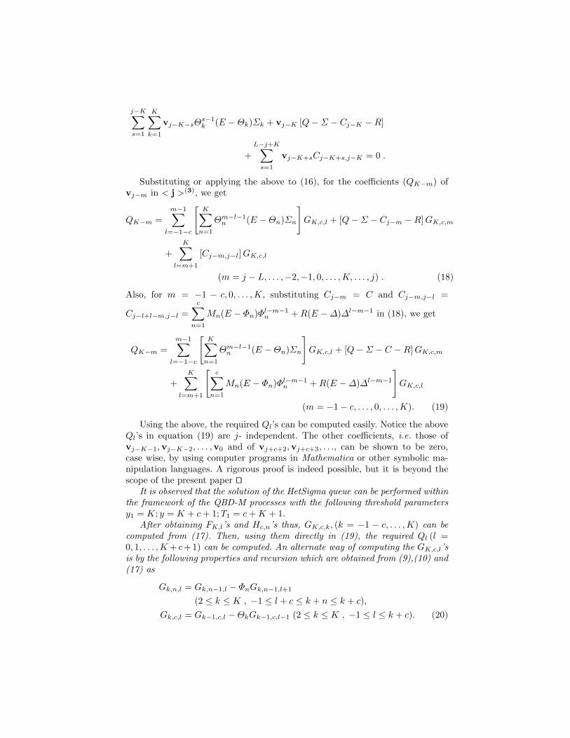
Substituting or applying the above to (16), for the coefficients (QK−m) ofvj−m in < j >(3), we get

QK−m =

m−1∑l=−1−c

[K∑n=1

Θm−l−1n (E −Θn)Σn

]GK,c,l + [Q−Σ − Cj−m −R]GK,c,m

+

K∑l=m+1

[Cj−m,j−l]GK,c,l

(m = j − L, . . . ,−2,−1, 0, . . . ,K, . . . , j) . (18)

Also, for m = −1 − c, 0, . . . ,K, substituting Cj−m = C and Cj−m,j−l =

Cj−l+l−m,j−l =

c∑n=1

Mn(E − Φn)Φl−m−1n +R(E −∆)∆l−m−1 in (18), we get

QK−m =

m−1∑l=−1−c

[K∑n=1

Θm−l−1n (E −Θn)Σn

]GK,c,l + [Q−Σ − C −R]GK,c,m

+

K∑l=m+1

[c∑

n=1

Mn(E − Φn)Φl−m−1n +R(E −∆)∆l−m−1

]GK,c,l

(m = −1− c, . . . , 0, . . . ,K). (19)

Using the above, the required Ql’s can be computed easily. Notice the aboveQl’s in equation (19) are j- independent. The other coefficients, i.e. those ofvj−K−1,vj−K−2, . . . ,v0 and of vj+c+2,vj+c+3, . . ., can be shown to be zero,case wise, by using computer programs in Mathematica or other symbolic ma-nipulation languages. A rigorous proof is indeed possible, but it is beyond thescope of the present paper ut

It is observed that the solution of the HetSigma queue can be performed withinthe framework of the QBD-M processes with the following threshold parametersy1 = K; y = K + c+ 1;T1 = c+K + 1.

After obtaining FK,l’s and Hc,n’s thus, GK,c,k, (k = −1 − c, . . . ,K) can becomputed from (17). Then, using them directly in (19), the required Ql (l =0, 1, . . . ,K+ c+ 1) can be computed. An alternate way of computing the GK,c,l’sis by the following properties and recursion which are obtained from (9),(10) and(17) as

Gk,n,l = Gk,n−1,l − ΦnGk,n−1,l+1

(2 ≤ k ≤ K , −1 ≤ l + c ≤ k + n ≤ k + c),

Gk,c,l = Gk−1,c,l −ΘkGk−1,c,l−1 (2 ≤ k ≤ K , −1 ≤ l ≤ k + c). (20)

Thus, the resulting equations (11) corresponding to the rows from c + K + 1to L− 2− c, are of the same form as those of the QBD-M processes and hencehave an efficient solution by several alternative methods such as the spectralexpansion method, Bini-Meini’s method [3] and the matrix-geometric methodswith folding and block-size enlargement. In our implementation, we have usedthe spectral expansion method. The required unknowns in the spectral expansionsolution and the steady state probabilities can be computed using the remainingbalance equations and the normalisation equation.

5 Applications

The HetSigma queue has been applied to evaluate performance problems intelecommunication systems [8, 23]. In this section, we present the application ofthe HetSigma queue to the performance analysis of MPLS networks which arebeing used in the backbone of IP networks.

5.1 A model for a multipath routing in MPLS networks

An example of an MPLS domain with routers and links is illustrated in Figure 1.Traffic demands traversing the MPLS domain are conveyed along pipes calledLabel Switched Paths (LSPs). When a packet arrives at the ingress router – aLabel Edge Router (LER) of the MPLS domain, the LER classifies incoming IP(or other packets for example Ethernet or even MPLS) packets to the appropriateFEC (Forward Equivalence Class) and encapsulates the packets within MPLSpackets. Labels are automatically assigned with the use of appropriate protocols,though labeling can also be allocated manually by the network administrator.A routing table (as the result of assignments of labels) in the LER is used toswitch packets in MPLS networks.

17

18

4

5

10

11

16

IngressRouter

EgressRouter

LSR

LSR

LSR

LSR

LSR

LSRLER

LER

LSP1

LSP2

LSP3

Fig. 1. MPLS domain

Servers

1

2

C

IP packets

Buffer

IngressRouter

EgressRouter

LSP1

LSP2

LSPc

Fig. 2. Model of an ingress node performing load balancing

In what follows, we describe the proposed model for an ingress-egress routerpair illustrated in Figure 2. Several paths can be defined and determined betweena given ingress-egress (IE) node pair in the MPLS network according to somepredefined criteria of the MPLS traffic engineering that is applied (e.g.: pathswith disjoint edges) for a single service class. Assume that there are c paths withdifferent bandwidths to be established between the IE node pair for a specificservice class. We model the c distinct paths (LSPs) in the system as the c distinctheterogeneous servers in parallel in the corresponding queuing model that weare introducing here for modeling the communication between the IE pair. TheLSPs in the network and the corresponding servers in the model are numberedin the same order. The GE-distributed service time parameters of the nth server(n = 1, 2 . . . , c) are denoted by (µn, φn) when the server is functional. L is thequeuing capacity (finite or infinite), in all phases, including the customers inservice, if any.

The packet arrival stream is represented by theMM∑Kk=1 CPPk arrival pro-

cess, this can accommodate traffic-burstiness, correlations among inter-arrivaltimes and correlations among batch sizes. It has been shown in the recentwork [21, 23] that the CPP is accurate enough to model real traffic (when CPPparameters are estimated from the captured traffic) and can be used for the per-

formance evaluation of real systems. The arrival process(the MM∑Kk=1 CPPk)

is inherently modulated by a CTMC X with N1 states, with generator matrixQX .

LSPs are prone to failures because of various reasons (e.g.: unreliable equip-ment, hardware failures, software bugs or cable cut). Such faults and failuresmay affect the operation of LSPs and cause packet losses and delays. In case offailures, the load balancing mechanism can move packets that are queued for theaffected LSPs to the unaffected LSPs.

When the failed link is repaired, the repaired LSP can be used again. Repairstrategy defines the order of repairing failed links, when there are more failedlinks than repairmen (it is assumed simultaneous repairs can happen). Repairstrategies can be preemptive or non-preemptive. However, it is not very realisticto apply a preemptive-priority repair strategy for the operation of networks inthe case of link cuts because of the travel cost of a maintenance team. In thispaper, we assume that one maintenance team is available to repair failures inthe network. However, the analysis can be easily extended to the case of multiplemaintenance facilities as well.

We consider four repair strategies, FCFS (First-Come-First-Served), LCFS(Last- Come-First-Served non-preemptive) and two based on link-priorities. Inthe strategies based on link-priorities, links with higher priorities should be setinto repair sooner, even if these failures have occurred later. The priority list oflinks may then be constructed in a greedy way, with a view to repair earlier thelink which would fetch larger gain in performance.

We assume the LSP states (or LSP configurations) that arise due to failuresand repairs of the LSPs can be described by a CTMC called Z. These LSP con-figurations would indeed correspond to all possible multi-server configurations(also termed, operative states of the multi-server) with functional as well asfailed servers, in the corresponding queuing model. This can well be so when ex-ponential or phase-type failures and repairs are assumed. Let N2, QZ denote thenumber of server-configurations and the generator matrix of the arising CTMCZ. Indeed N2 and QZ would depend on the parameters of the parallel servers,number of repairmen and the repair strategy.

In the presence of one repair team, we would need N2 =∑cl=0 Pe(c, l) = 2c+1

operative states for FCFS and LCFS repair strategies, where Pe(c, l) is thenumber of permutations of c distinct elements taken l at a time. Pe(c, l) = c!

(c−l)! .

Let ξk and ηk be the failure and repair rates respectively, of the kth LSP (that is,kth server in the multi-server model). Then QZ can be determined (illustrationfor c = 3 is presented below). Many other repair strategies can also be modeled,however, that is not in the scope of the present paper.

Both the arrival and the service processes can be thought of being jointlymodulated by the same continuous time, irreducible Markov process, with Nstates where N = N1 ·N2. That generator matrix of this joint modulating processis denoted by Q where Q is determined as

Q = QZ⊕

QX . (21)

Let the random variable I1(t) (1 ≤ I1(t) ≤ N1) represent the phase of the mod-ulating process X at any time t. We introduce I2(t) – an integer-valued randomvariable to describe the server configuration of the model (which correspondsto the network state) at time t. We define the following function,

γ(I2(t), n) =

{1 the nth server is functional0 otherwise

. (22)

The state I(t) (1 ≤ I(t) ≤ N ; N = N1 · N2) of the joint modulating pro-cess is constructed by lexicographically sorting the two variables (I1(t), I2(t)) asillustrated in Table 1.

Table 1. Order of the phase variable

I 1 2 . . . N1 N1 + 1 . . . 2N1 . . . N1N2 −N1 + 1 . . . N1N2

(I1, I2) (1, 1) (2, 1) . . . (N1, 1) (1, 2) . . . (N1, 2) . . . (1, N2) . . . (N1, N2)

From table 1, we can write the following equations,

I(t) = I1(t) + (I2(t)− 1)N1, I2(t) = f2(I(t)) =

⌊I(t)− 1

N1

⌋+ 1,

I1(t) = f1(I(t)) = [(I(t)− 1) mod N1] + 1. (23)

Consequently, the parameters of the arrival process are mapped as follows.The parameters of the GE inter-arrival time distribution of the kth (1 ≤ k ≤ K)customer arrival stream in phase i (i = 1, ..., N) are (σf1(i),k, θf1(i),k). The service

time parameters of the nth server (n = 1, 2, ..., c) in phase i (1 ≤ i ≤ N), denotedby (µi,n, φi,n) can be determined as,

µi,n = γ(f2(i), n)µn , φi,n = γ(f2(i), n)φn. (24)

5.2 Numerical results

An elaborate case study is carried out to determine the performance of a spe-cific ingress-egress node pair in an European Optical Network topology [1]. Thenetwork in Figure 3 contains 19 nodes and 78 optical links.

Traffic to the ingress node to be carried to the egress node, shown in thefigure, is assumed follow the ON- OFF process with two states (ON − OFF ).The ON and OFF periods are exponentially distributed with mean 0.4 and 0.5s respectively. The distribution of inter-arrival times in state ON is GE withparameters (σ = 150.6698990 (1/s), θ = 0.526471). In state OFF no packetsarrive. These parameters of the arrival stream are indeed derived from the inter-arrival times of the recorded samples of the real Bellcore traffic trace BC-pAug89[2], by matching the mean and variance.

Assume that there are three LSPs established between node 11 (ingress) andnode 4 (egress) of the IP/MPLS network as seen in Figure 3. The first LSP isrouted through nodes 10 and 5. The second LSP goes through nodes 17 and16, while the third one is through node 9. Thus, we have, in the model, c = 3servers with GE service time parameters (µi, φi (i = 1, 2, 3)) given by, µ1 = 96(1/s), µ2 = 128 (1/s), µ3 = 160 (1/s); φ1 = φ2 = φ3 = 0.109929. Note that

17

0

18

1

2

3

4

5

6

7

8

9

10

11

12

13

14

15

16

IngressRouter

EgressRouter

0.0004

0.0002

0.0001 0.0006

0.0003

0.0005

0.0002

0.0003

Fig. 3. Network topology

these parameters are obtained, based on the service capacity of the LSPs andthe packet lengths from the trace.

A specific LSP fails when a link through which the LSP is routed becomesinoperative (e.g.: cable cut). Normally, the failure rate of each link can be as-sumed to depend on its length. Using simple calculations, the failure rates areobtained as ξ1 = 0.001, ξ2 = 0.001 and ξ3 = 0.0006. The repair rate values (η1,η2 and η3) are chosen in such a way to have the availability of the connectivityensured by the LSPs between the ingress and egress node to be 99.9%.

Four repair strategies are compared in this section as follows. Note that afterthe identifications of LSP configurations in each strategy, the corresponding QZmatrices can be easily determined.

FCFS repairs It can be seen that there would be 16 LSP configurations or op-erative states represented as: (0, 0, 0)1,2,3, (0, 0, 0)1,3,2, (0, 0, 0)2,1,3, (0, 0, 0)2,3,1,(0, 0, 0)3,1,2, (0, 0, 0)3,2,1, (0, 0, 1)1,2, (0, 0, 1)2,1, (0, 1, 0)1,3, (0, 1, 0)3,1, (1, 0, 0)2,3,(1, 0, 0)3,2, (0, 1, 1), (1, 0, 1), (1, 1, 0) and (1, 1, 1). Here, the kth bit from leftwithin the brackets, is 0 when LSP k is broken, 1 when operative. Also,the suffix indicates the order in which the failed LSPs are to be repaired,if they are greater than one. If the above order is numbered from 0 to 15,then the nonzero and off- diagonal elements of matrix QZ can be given by,QZ(0, 10) = QZ(1, 11) = QZ(6, 13) = η1, QZ(8, 14) = QZ(12, 15) = η1,QZ(2, 8) = QZ(3, 9) = QZ(7, 12) = η2, QZ(10, 14) = QZ(13, 15) = η2,QZ(4, 6) = QZ(5, 7) = QZ(9, 12) = η3, QZ(11, 13) = QZ(14, 15) = η3,QZ(10, 3) = QZ(11, 5) = QZ(13, 7) = ξ1, QZ(14, 9) = QZ(15, 12) = ξ1,QZ(8, 1) = QZ(9, 4) = QZ(12, 6) = ξ2, QZ(14, 11) = QZ(15, 13) = ξ2,QZ(6, 0) = QZ(7, 2) = QZ(12, 8) = ξ3, and QZ(13, 10) = QZ(15, 14) = ξ3.

In the above, for example, the state (1, 0, 0)2,3 means that LSP 1 is functional,LSPs 2 and 3 are broken, the single repairman is working on LSP 2. From thisstate, the possible next states are (0, 0, 0)2,3,1 which happens by the failure ofLSP 1, or, (1, 1, 0) which happens by the repair of LSP 2. These are shown in QZas, QZ(10, 3) = ξ1, QZ(10, 14) = η2. All other elements of QZ can be explainedin a similar way.

5e−005

0.0002

0.0008

0.0032

0.0128

0.0512

110 130 150 170 190

Pac

ket

loss

pro

bab

ilit

y

Arrival intensity

Prior1 strategyPrior2 strategy

Fig. 4. Packet loss probability versus arrival rate

1.4

1.8

2.2

2.6

3

3.4

3.8

110 130 150 170 190

Queu

e le

ngth

Arrival intensity

Prior1 strategyPrior2 strategy

Fig. 5. Mean queue length versus arrival intensity

LCFS In this LCFS non-preemptive repair strategy, the repairman chooses thefailed server according to the LCFS discipline, and a repair is never preempted

by a new breakdown. Following the same representation and order as in FCFSstrategy, the non zero and off-diagonal elements of matrix QZ , in this case, can beobtained as, QZ(0, 10) = QZ(1, 11) = QZ(6, 13) = η1, QZ(8, 14) = QZ(12, 15) =η1, QZ(2, 8) = QZ(3, 9) = QZ(7, 12) = η2, QZ(10, 14) = QZ(13, 15) = η2,QZ(4, 6) = QZ(5, 7) = QZ(9, 12) = η3, QZ(11, 13) = QZ(14, 15) = η3,QZ(10, 2) = QZ(11, 4) = QZ(13, 7) = ξ1, QZ(14, 9) = QZ(15, 12) = ξ1,QZ(8, 0) = QZ(9, 5) = QZ(12, 6) = ξ2, QZ(14, 11) = QZ(15, 13) = ξ2,QZ(6, 1) = QZ(7, 3) = QZ(12, 8) = ξ3, and QZ(13, 10) = QZ(15, 14) = ξ3.

Priority-based strategy In a LSP-priority based repair strategy, it can becrucial to determine the priority of links according to which failed links are tobe repaired. In this section, we try to derive a decision function based on systemparameters to decide upon the priorities of the failed links.

Let fi and ri be the failure and repair rates of link i respectively and bi, itsbandwidth. The bandwidth of a link is computed from the summation of theLSPs bandwidths passing through this particular link. This approach ensuresthat links used by several LSPs may get higher priority, over the links used onlyby one LSP, when the former has larger bandwidth contribution. The wi, theweight of link i is set to

wi =rifi∗ bi. (25)

A repair strategy called Prior1 is based entirely on the failure rate of thelinks. That is, when there are several failed links, the link with a smallest failurerate is set into repair by the single repair facility available. Another strategycalled Prior2 is based on the decision function (wi). If wi > wk, then link i isgiven higher repair priority than link k in Prior2.

To compare Prior1 and Prior2, we plot the curves concerning packet lossand average number of customers waiting in the queue are versus the arrival rateof packets in Figure 4 and 5, respectively. We can observe that applying Prior2repair strategy results in a better performance characteristics than Prior1. ThePrior2 strategy takes more information into account about the network linkstowards the decision of repair order which can explain the better results. Itbalances not only failure rates, but also the repair rates and the bandwidthof links used by the passing-through LSPs. Therefore, we will only investigatestrategies FCFS, LCFS and Prior2 (will be referred as priority strategy) in whatfollows.

We now examine the effect of the repair rate of optical links on the perfor-mance of the system. In order to ensure that the availability of service betweenthe ingress and egress node to lie between 99.9% and 99.999%, it can be shownthat the repair rate should be in the interval [0.0397703,0.405355]. We investi-gate the effect of the repair rate of link within that range, on the performance.The expected queue length was reduced only by a small extent by the increaseof repair rate (see Figure 6). The packet-loss probability varied nearly in inverse-proportion to the repair rate (see Figure 7). Of course, the results would actually

3.4

3

2.6

2.2

1.8

0.035 0.03 0.025 0.02 0.015 0.01

Que

ue le

ngth

Repair rate

LCFS strategyFCFS strategy

Priority strategy

Fig. 6. Mean queue length versus the repair rate

0.0512

0.0128

0.0032

0.0008

0.0002

0.035 0.03 0.025 0.02 0.015 0.01

Pack

et lo

ss p

roba

bilit

y

Repair rate

LCFS strategyFCFS strategy

Priority strategy

Fig. 7. Packet loss probability versus the repair rate

depend on many other factors too including the load in the network. Accurateestimation of the returns on investment that is used to increase repair rate can bemade, only if the cost-patterns involved in increasing the repair rate are known.It may also be observed, in the considered range of experimentation, the variousrepair strategies considered do not have significant impact on the performanceand the availability of the service in the network (in the range of repair ratesthat are considered).

Figures 8 and 9, where the strategies are compared versus the arrival ratealso confirm an observation that the priority based repair outperforms the LCFSand FCFS ones.

5e−005

0.0002

0.0008

0.0032

0.0128

0.0512

110 130 150 170 190

Pac

ket

loss

pro

bab

ilit

y

Arrival intensity

Priority strategyFCFS strategyLCFS strategy

Fig. 8. Packet loss probability versus arrival rate

1.4

1.8

2.2

2.6

3

3.4

3.8

110 130 150 170 190

Queu

e le

ngth

Arrival intensity

Priority strategyFCFS strategyLCFS strategy

Fig. 9. Mean queue length versus arrival intensity

6 Extensions

6.1 Other killing disciplines

Apart from the killing discipline that was used above, there are two other popularkilling disciplines, the RCE-inimmune servicing and the RCH killing disciplines.The applicability of the killing disciplines rather depends on the situation andthe purpose, and hence depending on these, many more killing disciplines aretheoretically possible. Our methodology can easily be extended to many otherkilling disciplines also, this is explained briefly in this section.

The RCE-inimmune discipline In the RCE-inimmune servicing, the nega-tive customer removes the most recent positive arrival regardless of whether it isin service or waiting; thus a negative arrival has no effect only when it encoun-ters an empty queue and all servers idle. This is the traditional killing discipline,suited to the modeling of killing signals in speculative parallelism, for example.It can also be used to model cell losses caused by the arrival of a corrupted cellor one encountering a full buffer, when the preceding cells of a packet would bediscarded. In this case, the later and the upward transitions remain as before,but the downward transition rates become [13]

Cj+s,j = C(E − Φ)Φs−1 +R(E −∆)∆s−1

(c ≤ j ≤ L− 1 ; s = 1, 2, . . . , L− j)= CΦs−1 +R(E −∆)∆s−1 (c > 1 ; j = c− 1 ; 1 ≤ s ≤ L− c+ 1)

= CΦs−1 +R∆s−1 (c = 1 ; j = c− 1 = 0 ; 1 ≤ s ≤ L)

= Cj+1 +R(E −∆) (1 ≤ j ≤ c− 2 ; s = 1)

= R(E −∆)∆s−1 (1 ≤ j ≤ c− 2 ; 2 ≤ s ≤ L− j)= R∆s−1 (c > 1 ; j = 0 ; 2 ≤ s ≤ L)

= C1 +R (j = 0 ; s = 1).

Thus, after obtaining the required transition rates, e.g. lateral, upward and down-ward, and the balance equations in this case, the same procedure can be used,perhaps with slight appropriate modifications, to transform the balance equa-tions to a suitable form (QBD-M type equations) for solving by the existingmethods.

The RCH discipline Another popular killing discipline is the RCH (Removalof customers from the head of the queue) killing discipline. This is appropriate formodeling server breakdowns, where a customer in service will be lost for sure andmay be also a portion of queue of waiting customers. Here too, the A matricesand the B matrices remain unchanged, however the C matrices would be differentand can be determined. For example, to obtain Cj+s,j , consider the system (say,a single server system with c = 1) in state (i, j + s), where j + s ≤ L. The rateat which a batch of l negative customers arrives is (1 − δi)δl−1i ρi (l = 1, 2, . . .).

If l ≥ j + s, then all the jobs will be removed by the negative customers. Ifl < j + s, then the job in service plus l − 1 jobs waiting for service would beremoved, leaving only j+s−l jobs. However, due to the nature of the generalizedexponential service times, a certain number of customers may be ’leaked out’,i.e. serviced instantaneously just after the killing takes place. Alternatively, ifwe redefine the operation of the system such that this leakage does not occur,i.e. immediately after a negative arrival, the next customer in the queue (if any)cannot skip service, then the equilibrium state probabilities would be same as inthe case of the RCE-inimmune servicing.

Assuming leakage, the rate matrices Cj+s,j can be derived as [13],

Cj+s,j = (E − Φ)Φs−1M + (E −∆)R(E − Φ){Φ∆}s−1(1 ≤ j ≤ L− 1 ; s ≥ 1) ;

= Φs−1M + (E −∆)R{Φ∆}s−1 +R∆s (j = 0 ; s ≥ 2) ;

= M +R (j = 0 ; s = 1) ;

where,

{Φ∆}s−1 =

s−1∑k=0

Φs−1−k∆k (s ≥ 2) ;

= E (s = 1) .

This case also can be modeled following the previous procedures, perhaps withminor modifications.

6.2 truncated-CPP(t-CPP)

By incorporating several CPP’s and superposing them, non-geometric batch sizearrivals could be modeled, to certain extent and with certain limitations. Thatflexibility can be increased, in fact greatly, by replacing the CPP’s by truncated-CPP’s (or t-CPP’s). The method of transforming the balance equation for ef-ficient solution may be applicable in principle, but with some modifications, tothis case as well and hence can be extended with some effort.

Let the parameters of the kth t-CPP in the ith phase be (σi,k, θi,k, bi,k, di,k),which means the batch size is geometrically distributed and bounded by bi,k asthe minimum batch size and di,k as the maximum. Also, the inter-arrival timebetween successive batches, during that modulating phase, is exponential withparameter σi,k. The probability of batch size being s of this t-CPP is then given

by(1−θi,k)θs−1

i,k

θbi,k−1

i,k −θdi,ki,k

if bi,k ≤ s ≤ di,k, 0 otherwise. Hence, the overall batch size

distribution in phase i arrivals is then modified as

πl/i =

K∑k=1

σi,kσi,.

(1− θi,k)θl−1i,k

θbi,k−1i,k − θdi,ki,k

fi,k,l, (26)

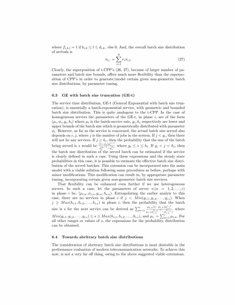
where fi,k,l = 1 if bi,k ≤ l ≤ di,k, else 0. And, the overall batch size distributionof arrivals is

πl/. =

N∑i=1

riπi,l. (27)

Clearly, the superposition of t-CPP’s (26, 27), because of larger number of pa-rameters and batch size bounds, offers much more flexibility than the superpo-sition of CPP’s in order to generate/model certain given non-geometric batchsize distributions, by parameter tuning.

6.3 GE with batch size truncation (GE-t)

The service time distribution, GE-t (General Exponential with batch size trun-cation), is essentially a batch-exponential service, with geometric and boundedbatch size distribution. This is quite analogous to the t-CPP. In the case ofhomogeneous servers the parameters of the GE-t, in phase i, are of the form(µi, φi, gi, hi) where µi is the batch-service rate, gi, hi respectively are lower andupper bounds of the batch size which is geometrically distributed with parameterφi. However, as far as the service is concerned, the actual batch size served alsodepends on c, j, where j is the number of jobs in the system. If j < gi, then therewill not be any services. If j ≥ hi, then the probability that the size of the batch

being served is s would be(1−φi)φ

s−1i

φgi−1

i −φhii

where gi ≤ s ≤ hi. If gi < j < hi, then

the batch size distribution of the served batch can be estimated if the serviceis clearly defined in such a case. Using these expressions and the steady stateprobabilities in this case, it is possible to estimate the effective batch size distri-bution of the served batches. This extension can be incorporated into the mainmodel with a viable solution following same procedures as before, perhaps withminor modifications. This modification can result in, by appropriate parametertuning, incorporating certain given non-geometric batch size services.

That flexibility can be enhanced even further if we use heterogeneousservers. In such a case, let the parameters of server n (n = 1, 2, . . . , c)in phase i be, (µi,n, φi,n, gi,n, hi,n). Extrapolating the earlier analyis to thiscase, there are no services in phase i if j < Min(gi,1, gi,2, . . . , gi,c). Whenj ≥ Max(hi,1, hi,2, . . . , hi,c) in phase i, then the probability that the batch

size is s for the next service can be derived as∑cn=1

µi,n(1−φi,n)φs−1i,n

µi.(φgi,n−1

i,n −φhi,ni,n )

where

Min(gi,1, gi,2, . . . , gi,c) ≤ s ≤Max(hi,1, hi,2, . . . , hi,c), and µi. =∑cn=1 µi,n. For

all other ranges or values of s, the expressions for the probability distributioncan be obtained.

6.4 Towards abritrary batch size distributions

The consideration of abritrary batch size distributions is most desirable in theperformance evaluation of modern telecommunication networks. To achieve thisnow, is not a very far off thing, owing to the above suggested viable extensions.

And thus, we arrive at a much more general and useful model, that is, the MM∑Kk=1 t− CPPk/GE-t/c/L G-queue with heterogeneous servers. Further work is

being carried out on this model.

7 Conclusions

The HetSigma queuing model is developed as a generalization of the QBD pro-cesses. In this queue, it is possible to accommodate inter-arrival time corre-lations, service time correlations, batch-size correlations, large and unboundedbatch sizes. All these aspects are useful in order to model emerging communica-tion systems. Certain non-trivial transformations are conceived on the balanceequations. The transformed balance equations are of the QBD-M type, hencethere is a fast solution using the spectral expansion method. The queue is ap-plied for the performance evaluation of MPLS networks with unreliable nodesand can be used to model various problems in telecommunication network aswell. It is possible to extend or further generalize these models to develop highlygeneralized Markovian node models for the emerging Next Generation Networks.That work is underway.

Acknowledgement Ram Chakka thanks the Chancellor of Sri Sathya Sai Uni-versity, Prasanthi Nilayam, India, for constant encouragement, guidance andinspiration throughout this work.

References

1. Network Research Topologies: The European optical network (EON).http://www.optical-network.com/topology.php.

2. The Internet traffic archive. http://ita.ee.lbl.gov/index.html.

3. D. Bini and B. Meini. On the solution of a nonlinear matrix equation arising inqueueing problems. SIAM Journal on Matrix Analysis and Applications, 17(4):906–926, 1996.

4. C. Blondia and O. Casals. Statical Multiplexing of VBR Source: A Matrix-AnalyticApproach. Performance Evaluation, 16:5–20, 1992.

5. Ram Chakka. Performance and Reliability Modelling of Computing Systems UsingSpectral Expansion. PhD thesis, University of Newcastle upon Tyne (Newcastleupon Tyne), 1995.

6. Ram Chakka. Spectral Expansion Solution for some Finite Capacity Queues. An-nals of Operations Research, 79:27–44, 1998.

7. Ram Chakka and Tien Van Do. The MM∑K

k=1 CPPk/GE/c/L G-Queue and ItsApplication to the Analysis of the Load Balancing in MPLS Networks. In 27thAnnual IEEE Conference on Local Computer Networks (LCN 2002), 6-8 November2002, Tampa, FL, USA, Proceedings, pages 735–736, 2002.

8. Ram Chakka and Tien Van Do. The MM∑K

k=1 CPPk/GE/c/L G-Queue withHeterogeneous Servers: Steady state solution and an application to performanceevaluation. Performance Evaluation, 64:191–209, March 2007.

9. Ram Chakka, Tien Van Do, and Zsolt Pandi. Generalized Markovian queues andapplications in performance analysis in telecommunication networks. In D. D. Kou-vatsos, editor, the First International Working Conference on Performance Mod-elling and Evaluation of Heterogeneous Networks (HET-NETs 03), pages 60/1–10,July 2003.

10. Ram Chakka, Tien Van Do, and Zsolt Pandi. A Generalized Markovian Queueand Its Applications to Performance Analysis in Telecommunications Networks.In D. Kouvatsos, editor, Performance Modelling and Analysis of HeterogeneousNetworks, pages 371–387. River Publisher, 2009.

11. Ram Chakka, Enver Ever, and Orhan Gemikonakli. Joint-state modeling for openqueuing networks with breakdowns, repairs and finite buffers. In 15th InternationalSymposium on Modeling, Analysis, and Simulation of Computer and Telecommu-nication Systems (MASCOTS ), pages 260–266. IEEE Computer Society, 2007.

12. Ram Chakka and Peter G. Harrison. Analysis of MMPP/M/c/L queues. In Pro-ceedings of the Twelfth UK Computer and Telecommunications Performance En-gineering Workshop, pages 117–128, Edinburgh, 1996.

13. Ram Chakka and Peter G. Harrison. The Markov modulated CPP/GE/c/L queuewith positive and negative customers. In Proceedings of the 7th IFIP ATM Work-shop, Antwerp, Belgium, 1999.

14. Ram Chakka and Peter G. Harrison. A Markov modulated multi-server queue withnegative customers - the MM CPP/GE/c/L G-queue. Acta Informatica, 37:881–919, 2001.

15. Ram Chakka and Peter G Harrison. The MMCPP/GE/c queue. Queueing Systems:Theory and Applications, 38:307–326, 2001.

16. Ram Chakka and Isi Mitrani. Multiprocessor systems with general breakdownsand repairs. In SIGMETRICS, pages 245–246, 1992.

17. Ram Chakka and Isi Mitrani. Heterogeneous multiprocessor systems with break-downs: Performance and optimal repair strategies. Theor. Comput. Sci., 125(1):91–109, 1994.

18. M. Chien and Y. Oruc. High performance concentrators and superconcentratorsusing multiplexing schemes. IEEE Transactions on Communications, 42:3045–3050, 1994.

19. D. Kouvatsos. Entropy Maximisation and Queueing Network Models. Annals ofOperations Research, 48:63–126, 1994.

20. Tien Van Do. Comments on multi-server system with single working vacation.Applied Mathematical Modelling, 33(12):4435–4437, 2009.

21. Tien Van Do, Ram Chakka, and Peter G. Harrison. An integrated analytical modelfor computation and comparison of the throughputs of the UMTS/HSDPA userequipment categories. In MSWiM ’07: Proceedings of the 10th ACM Symposiumon Modeling, analysis, and simulation of wireless and mobile systems, pages 45–51,New York, NY, USA, 2007. ACM.

22. Tien Van Do, Nam H. Do, and Ram Chakka. Performance evaluation of the highspeed downlink packet access in communications networks based on high altitudeplatforms. In Khalid Al-Begain, Armin Heindl, and Miklos Telek, editors, ASMTA,volume 5055 of Lecture Notes in Computer Science, pages 310–322. Springer, 2008.

23. Tien Van Do, Udo R. Krieger, and R. Chakka. Performance modeling of an apacheweb server with a dynamic pool of service processes. Telecommunication Systems,39(2):117–129, 2008.

24. Tien Van Do, Denes Papp, Ram Chakka, and Mai X T Truong. A PerformanceModel of MPLS Multipath Routing with Failures and Repairs of the LSPs. In

D. Kouvatsos, editor, Performance Modelling and Analysis of Heterogeneous Net-works, pages 27–43. River Publisher, 2009.

25. Steve Drekic and Winfried K. Grassmann. An eigenvalue approach to analyzing afinite source priority queueing model. Annals OR, 112(1-4):139–152, 2002.

26. R. V. Evans. Geometric Distribution in some Two-dimensional Queueing Systems.Operations Research, 15:830–846, 1967.

27. Enver Ever, Orhan Gemikonakli, and Ram Chakka. A mathematical model forperformability of beowulf clusters. In Annual Simulation Symposium, pages 118–126. IEEE Computer Society, 2006.

28. Enver Ever, Orhan Gemikonakli, and Ram Chakka. Analytical modelling and simu-lation of small scale, typical and highly available beowulf clusters with breakdownsand repairs. Simulation Modelling Practice and Theory, 17(2):327–347, 2009.

29. R.J. Fretwell and D.D. Kouvatsos. ATM traffic burst lengths are geometricallybounded. In Proceedings of the 7 th IFIP Workshop on Performance Modellingand Evaluation of ATM & IP Networks, Antwerp, Belgium, 1999. Chapman andHall.

30. H. R. Gail, S. L. Hantler, and B. A. Taylor. Spectral analysis of M/G/1 typeMarkov chains. Technical Report RC17765, IBM Research Division, 1992.

31. Winfried K. Grassmann. The use of eigenvalues for finding equilibrium probabilitiesof certain markovian two-dimensional queueing problems. INFORMS Journal onComputing, 15(4):412–421, 2003.

32. Winfried K. Grassmann and Steve Drekic. An analytical solution for a tandemqueue with blocking. Queueing System, (1-3):221–235, 2000.

33. B. Haverkort and A. Ost. Steady State Analysis of Infinite Stochastic Petri Nets:A Comparing between the Spectral Expansion and the Matrix Geometric Method.In Proceedings of the 7th International Workshop on Petri Nets and PerformanceModels, pages 335–346, 1997.

34. ITU-T Recommendation Y.2001. General overview of NGN, 2005. Geneve,Switzerland.

35. D. D. Kouvatsos. A maximum entropy analysis of the G/G/1 Queue at Equilib-rium. Journal of Operations Research Society, 39:183–200, 1998.

36. U. R. Krieger, V. Naoumov, and D. Wagner. Analysis of a Finite FIFO Buffer inan Advanced Packet-Switched Network. IEICE Trans. Commun., E81-B:937–947,1998.

37. G. Latouche and V. Ramaswami. Introduction to Matrix Analytic Methods inStochastic Modeling. ASA-SIAM Series on Statistics and Applied Probability, 1999.

38. Isi Mitrani. Approximate solutions for heavily loaded markov-modulated queues.Perform. Eval., 62(1-4):117–131, 2005.

39. Isi Mitrani and Ram Chakka. Spectral expansion solution for a class of Markovmodels: Application and comparison with the matrix-geometric method. Perfor-mance Evaluation, 23:241–260, 1995.

40. V. Naoumov, U. R. Krieger, and D. Warner. Analysis of a Multi-Server Delay-LossSystem With a General Markovian Arrival Process. In S. R. Chakravarthy andA. S. Alfa, editors, Matrix-analytic methods in stochastic models, volume 183 ofLecture Notes in Pure and Applied Mathematics. Marcel Dekker, September 1996.

41. M. F. Neuts. Matrix Geometric Soluctions in Stochastic Model. Johns HopkinsUniversity Press, Baltimore, 1981.

42. Z. Niu and Y. Takahashi. An Extended Queueing Model for SVC-based IP-over-ATM Networks and its Analysis. In Proceedings of IEEE GLOBECOM, pages490–495, 1998.

43. I. Norros. A Storage Model with Self-similar Input. Queueing Systems and theirApplications, 16:387–396, 1994.

44. V. Paxman and S. Floyd. Wide-area traffic: The failure of Poisson modelling.IEEE/ACM Transactions on Networking, 3(3):226–244, 1995.

45. Emilia Rosti, Evgenia Smirni, and Kenneth C. Sevcik. On processor saving schedul-ing policies for multiprocessor systems. IEEE Trans. Comp, 47:47–2, 1998.

46. L. P. Seelen. An Algorithm for Ph/Ph/c queues. European Journal of OperationalResearch, 23:118–127, 1986.

47. Charalambos Skianis and Demetres Kouvatsos. An Information Theoretic Ap-proach for the Performance Evaluation of Multihop Wireless Ad Hoc Networks. InD. D. Kouvatsos, editor, Proceedings of the Second International Working Confer-ence on Performance Modelling and Evaluation of Heterogeneous Networks (HET-NETs 04), pages P81/1–13, Ilkley, UK, July 2004.

48. W. J. Stewart. Introduction to Numerical Solution of Markov Chains. PrincetonUniversity Press, 1994.

49. H. T. Tran and T. V. Do. An iterative method for queueing systems with batcharrivals and batch departures. In Proceedings of the 8th IFIP Workshop on Per-formance Modelling and Evaluation of ATM&IP Networks, pages 80/1–13, Ilkley,UK, 2000.

50. H. T. Tran and T. V. Do. A new iterative method for systems with batch arrivalsand batch departures. In Proceedings of CNDS’00, pages 131–137, San Diego, USA,2000.

51. H. T. Tran, T. V. Do, and T. Ziegler. Analysis of MPLS-compliant Nodes De-ploying Multiple LSPs Routing. In Proceedings of the First International WorkingConference on Performance Modelling and Evaluation of Heterogeneous Networks,HET-NETs, pages 26/1–26/10, July, 2003.

52. Hung T. Tran and Tien Van Do. Computational Aspects for Steady State Analysisof QBD Processes . Periodica Polytechnica, Ser. El. Eng, pages 179–200, 2000.

53. Hung T. Tran and Tien Van Do. Generalised invariant Subspace based Method forSteady State Analysis of QBD-M Proceses. Periodica Polytechnica, Ser. El. Eng.,44:159–178, 2000.

54. Hung T. Tran and Tien Van Do. Comparison of some Numerical Methods for QBD-M Processes via Analysis of an ATM Concentrator. In Proceedings of 20th IEEEInternational Performance, Computing and Communications Conference, IPCCC2001, Pheonix, USA, 2001.

55. V. L. Wallace. The Solution of Quasi Birth and Death Processes Arising frommultiple Access Computer Systems. PhD thesis, University of Michigan, 1969.

56. Adam Wierman, Takayuki Osogami, Mor Harchol-Balter, and Alan Scheller-Wolf.How many servers are best in a dual-priority M/PH/k system? Perform. Eval.,63(12):1253–1272, 2006.

57. Patrick Wuchner, Janos Sztrik, and Hermann de Meer. Finite-source M/M/S re-trial queue with search for balking and impatient customers from the orbit. Com-puter Networks, 53(8):1264–1273, 2009.

58. Y. Zhao and Winfried K. Grassmann. A numerically stable algorithm for twoserver queue models. Queueing Syst., 8(1):59–79, 1991.