GENERALIZED PICARD CONDITION ANALYSIS

FOR ESTIMATING PARAMETERS IN THE SPLIT

BREGMAN ALGORITHM FOR NOISY DATA

Rosemary Renauthttp://math.asu.edu/˜rosie

SIAM IMAGING

MAY, 2012THANKS TO:

OCCAM OXFORD AND CHARLES UNIVERSITY PRAGUE

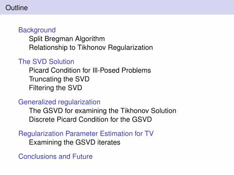
Outline

BackgroundSplit Bregman AlgorithmRelationship to Tikhonov Regularization

The SVD SolutionPicard Condition for Ill-Posed ProblemsTruncating the SVDFiltering the SVD

Generalized regularizationThe GSVD for examining the Tikhonov SolutionDiscrete Picard Condition for the GSVD

Regularization Parameter Estimation for TVExamining the GSVD iterates

Conclusions and Future

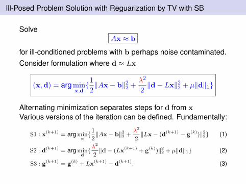
Ill-Posed Problem Solution with Reguarization by TV with SB

SolveAx ≈ b

for ill-conditioned problems with b perhaps noise contaminated.Consider formulation where d ≈ Lx

(x,d) = arg minx,d{1

2‖Ax− b‖22 +

λ2

2‖d− Lx‖22 + µ‖d‖1}

Alternating minimization separates steps for d from x

Various versions of the iteration can be defined. Fundamentally:

S1 : x(k+1) = argminx{12‖Ax− b‖22 +

λ2

2‖Lx− (d(k+1) − g(k))‖22} (1)

S2 : d(k+1) = argmind{λ

2

2‖d− (Lx(k+1) + g(k))‖22 + µ‖d‖1} (2)

S3 : g(k+1) = g(k) + Lx(k+1) − d(k+1). (3)

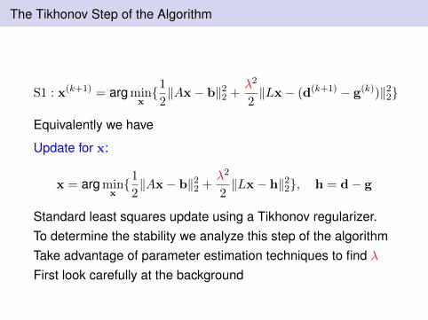
The Tikhonov Step of the Algorithm

S1 : x(k+1) = arg minx{1

2‖Ax− b‖22 +

λ2

2‖Lx− (d(k+1) − g(k))‖22}

Equivalently we have

Update for x:

x = arg minx{1

2‖Ax− b‖22 +

λ2

2‖Lx− h‖22}, h = d− g

Standard least squares update using a Tikhonov regularizer.To determine the stability we analyze this step of the algorithmTake advantage of parameter estimation techniques to find λFirst look carefully at the background

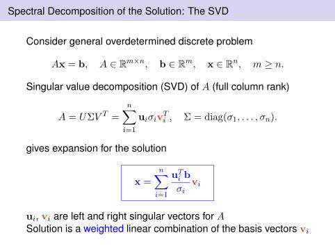
Spectral Decomposition of the Solution: The SVD

Consider general overdetermined discrete problem

Ax = b, A ∈ Rm×n, b ∈ Rm, x ∈ Rn, m ≥ n.

Singular value decomposition (SVD) of A (full column rank)

A = UΣV T =

n∑i=1

uiσivTi , Σ = diag(σ1, . . . , σn).

gives expansion for the solution

x =

n∑i=1

uTi b

σivi

ui, vi are left and right singular vectors for ASolution is a weighted linear combination of the basis vectors vi

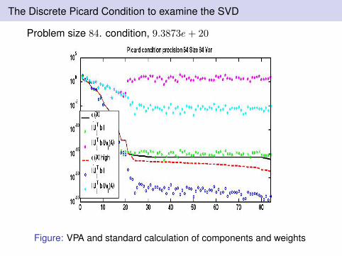
The Discrete Picard Condition to examine the SVD

Problem size 84. condition, 9.3873e+ 20

Figure: VPA and standard calculation of components and weights

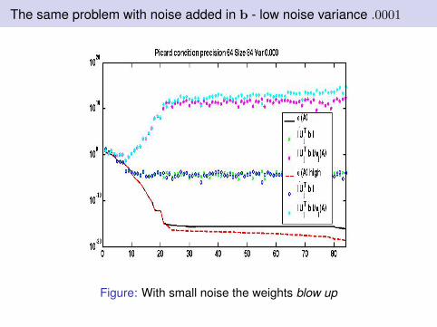
The same problem with noise added in b - low noise variance .0001

Figure: With small noise the weights blow up

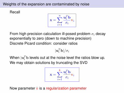
Weights of the expansion are contaminated by noise

Recall

x =

n∑i=1

uTi b

σivi

From high precision calculation ill-posed problem σi decayexponentially to zero (down to machine precision)Discrete Picard condition: consider ratios

|uTi b|/σi

When |uTi b levels out at the noise level the ratios blow up.We may obtain solutions by truncating the SVD

x =k∑i=1

uTi b

σivi

Now parameter k is a regularization parameter

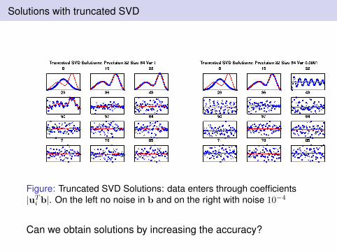
Solutions with truncated SVD

Figure: Truncated SVD Solutions: data enters through coefficients|uT

i b|. On the left no noise in b and on the right with noise 10−4

Can we obtain solutions by increasing the accuracy?

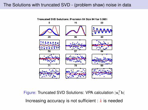
The Solutions with truncated SVD - (problem shaw) noise in data

Figure: Truncated SVD Solutions: VPA calculation |uTi b|

Increasing accuracy is not sufficient : k is needed

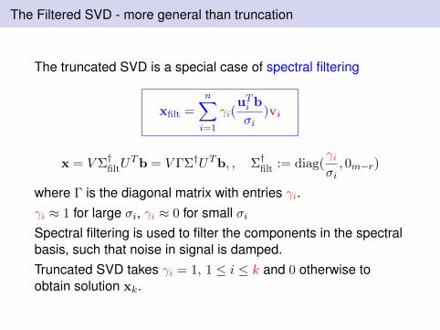
The Filtered SVD - more general than truncation

The truncated SVD is a special case of spectral filtering

xfilt =

n∑i=1

γi(uTi b

σi)vi

x = V Σ†filtUTb = V ΓΣ†UTb, , Σ†filt := diag(

γiσi, 0m−r)

where Γ is the diagonal matrix with entries γi.γi ≈ 1 for large σi, γi ≈ 0 for small σiSpectral filtering is used to filter the components in the spectralbasis, such that noise in signal is damped.Truncated SVD takes γi = 1, 1 ≤ i ≤ k and 0 otherwise toobtain solution xk.

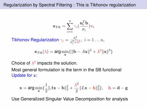
Regularization by Spectral Filtering : This is Tikhonov regularization

xTik =

n∑i=1

γi(uTi b

σi)vi

Tikhonov Regularization γi =σ2i

σ2i +λ2

, i = 1 . . . n,

xTik(λ) = arg minx{‖b−Ax‖2 + λ2‖x‖2}

Choice of λ2 impacts the solution.Most general formulation is the term in the SB functionalUpdate for x:

x = arg minx{1

2‖Ax− b‖22 +

λ2

2‖Lx− h‖22}, h = d− g

Use Generalized Singular Value Decomposition for analysis

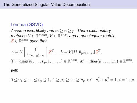
The Generalized Singular Value Decomposition

Lemma (GSVD)Assume invertibility and m ≥ n ≥ p. There exist unitarymatrices U ∈ Rm×m, V ∈ Rp×p, and a nonsingular matrixZ ∈ Rn×n such that

A = U

[Υ

0(m−n)×n

]ZT , L = V [M, 0p×(n−p)]Z

T ,

Υ = diag(υ1, . . . , υp, 1, . . . , 1) ∈ Rn×n, M = diag(µ1, . . . , µp) ∈ Rp×p,

with

0 ≤ υ1 ≤ · · · ≤ υp ≤ 1, 1 ≥ µ1 ≥ · · · ≥ µp > 0, υ2i + µ2

i = 1, i = 1 : p.

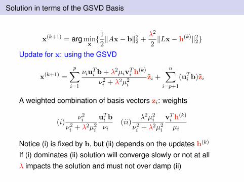
Solution in terms of the GSVD Basis

x(k+1) = arg minx{1

2‖Ax− b‖22 +

λ2

2‖Lx− h(k)‖22}

Update for x: using the GSVD

x(k+1) =

p∑i=1

νiuTi b + λ2µiv

Ti h

(k)

ν2i + λ2µ2

i

zi +

n∑i=p+1

(uTi b)zi

A weighted combination of basis vectors zi: weights

(i)ν2i

ν2i + λ2µ2

i

uTi b

νi(ii)

λ2µ2i

ν2i + λ2µ2

i

vTi h(k)

µi

Notice (i) is fixed by b, but (ii) depends on the updates h(k)

If (i) dominates (ii) solution will converge slowly or not at allλ impacts the solution and must not over damp (ii)

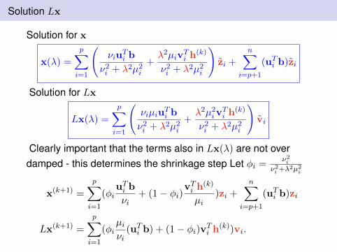
Solution Lx

Solution for x

x(λ) =

p∑i=1

(νiu

Ti b

ν2i + λ2µ2

i

+λ2µiv

Ti h

(k)

ν2i + λ2µ2

i

)zi +

n∑i=p+1

(uTi b)zi

Solution for Lx

Lx(λ) =

p∑i=1

(νiµiu

Ti b

ν2i + λ2µ2

i

+λ2µ2

ivTi h

(k)

ν2i + λ2µ2

i

)vi

Clearly important that the terms also in Lx(λ) are not overdamped - this determines the shrinkage step Let φi =

ν2iν2i +λ2µ2i

x(k+1) =

p∑i=1

(φiuTi b

νi+ (1− φi)

vTi h(k)

µi)zi +

n∑i=p+1

(uTi b)zi

Lx(k+1) =

p∑i=1

(φiµiνi

(uTi b) + (1− φi)vTi h(k))vi.

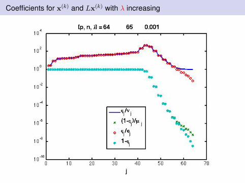
Coefficients for x(k) and Lx(k) with λ increasing

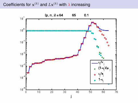
Coefficients for x(k) and Lx(k) with λ increasing

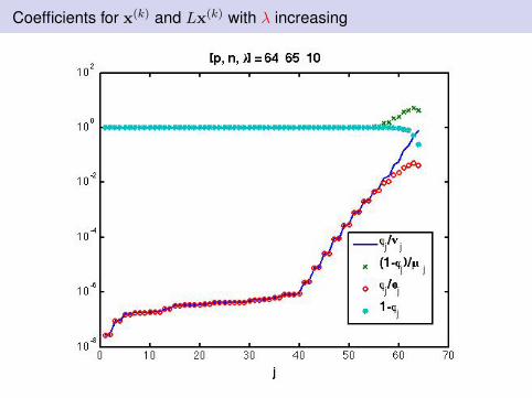
Coefficients for x(k) and Lx(k) with λ increasing

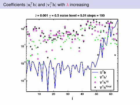
Coefficients |uTi b| and |vTi h| with λ increasing

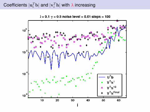
Coefficients |uTi b| and |vTi h| with λ increasing

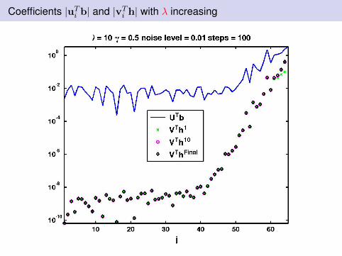
Coefficients |uTi b| and |vTi h| with λ increasing

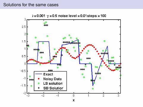
Solutions for the same cases

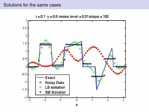
Solutions for the same cases

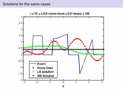
Solutions for the same cases

Observations: I

Discrete Picard condition analysis is relevantThe weights on both x and Lx are crucial to avoid stagnationλ needs to be chosen appropriatelyWealth of possibilities for choosing λ from standard Tikhonovregularization.Examples here will use Unbiased Predictive Risk Estimation -assume variance of noise in b is known.

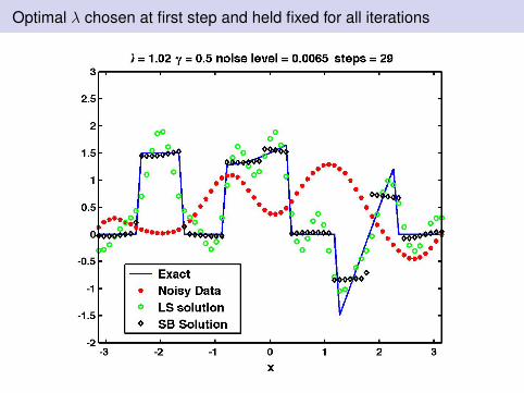
Optimal λ chosen at first step and held fixed for all iterations

Observation II

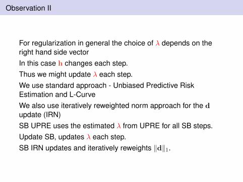
For regularization in general the choice of λ depends on theright hand side vectorIn this case h changes each step.Thus we might update λ each step.We use standard approach - Unbiased Predictive RiskEstimation and L-CurveWe also use iteratively reweighted norm approach for the dupdate (IRN)SB UPRE uses the estimated λ from UPRE for all SB steps.Update SB, updates λ each step.SB IRN updates and iteratively reweights ‖d‖1.

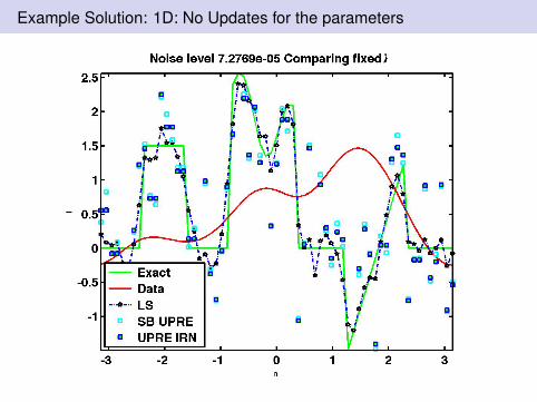
Example Solution: 1D: No Updates for the parameters

Figure: γ = 200 Low noise. Without updating λ left and updated right.SB UPRE uses the estimated λ from UPRE for all SB steps. UpdateSB, updates λ each step. SB IRN updates and iteratively reweights‖d‖1.

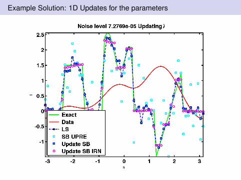
Example Solution: 1D Updates for the parameters

Figure: γ = 200 Low noise. Without updating λ left and updated right.SB UPRE uses the estimated λ from UPRE for all SB steps. UpdateSB, updates λ each step. SB IRN updates and iteratively reweights‖d‖1.

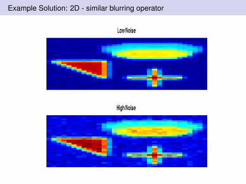
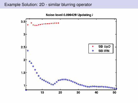
Example Solution: 2D - similar blurring operator

SB with updated λ is useful: This uses fixed ratio λ2/µ = 5

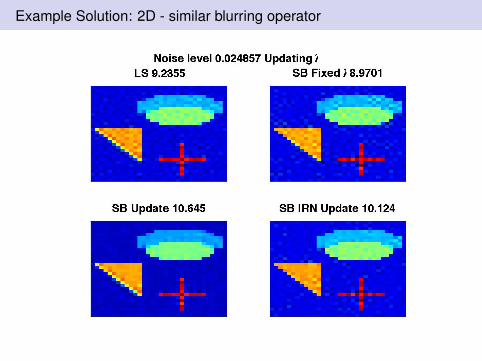
Example Solution: 2D - similar blurring operator

SB with updated λ is useful: This uses fixed ratio λ2/µ = 5

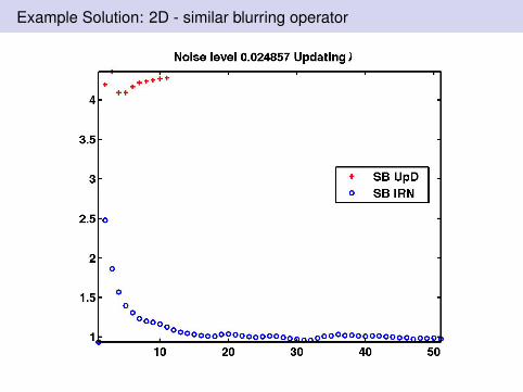
Example Solution: 2D - similar blurring operator

SB with updated λ is useful: This uses fixed ratio λ2/µ = 5

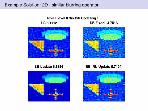
Example Solution: 2D - similar blurring operator

SB with updated λ is useful: This uses fixed ratio λ2/µ = 5

Example Solution: 2D - similar blurring operator

SB with updated λ is useful: This uses fixed ratio λ2/µ = 5

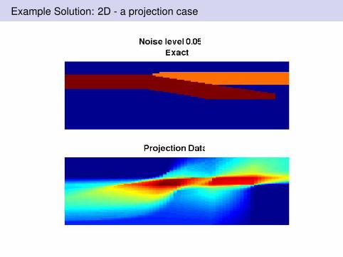
Example Solution: 2D - a projection case

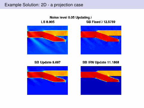
Example Solution: 2D - a projection case

Example Solution: 2D - a projection case

Further Observations and Future Work

Results demonstrate basic analysis of problem isworthwhile

Parameter estimation from basic LS should be used to findappropriate parameter at least at step 1

Overhead of optimal λ for the first step - reasonableOverhead of subsequent steps - UPRE requires matrix trace

- but can be optimized, or use χ2 approach Takesaccount of covariance on h

Convergence testing is based on h.IRN Reweighting needs some further work - converges

too slowlyFuture validate heuristics for more practical cases.

PSF Fourier Analysis for Decomposition of the Solution.