www.eprg.group.cam.ac.uk

EP

RG

WO

RK

ING

PA

PE

R

Abstract

Generalized Nash Equilibrium and Market Coupling in the European Power System

EPRG Working Paper 1016

Cambridge Working Paper in Economics 1034

Yves Smeers, Giorgia Oggioni, Elisabetta Allevi and Siegfried Schaible

"Market Coupling'' is currently seen as the most advanced market

design in the restructuring of the European electricity market. Market

coupling, by construction, introduces what is generally referred to as an

incomplete market: it leaves several constraints out of the market and

hence avoids pricing them. This may or may not have important

consequences in practice depending on the case on hand. Quasi-

Variational Inequality problems and the associated Generalized Nash

Equilibrium can be used for representing incomplete markets. Recent

papers propose methods for finding a set of solutions of Quasi-

Variational Inequality problems. We apply one of these methods to a

subproblem of market coupling namely the coordination of counter-

trading. This problem is an illustration of a more general question

encountered for instance in hierarchical planning in production

management. We first discuss the economic interpretation of the Quasi-

Variational Inequality problem. We then apply the algorithmic approach

to a set of stylized case studies in order to illustrate the impact of

different organizations of counter-trading. The paper emphazises the

structuring of the problem. A companion paper considers the full

problem of market coupling and counter-trading and presents a more

extensive numerical analysis.

www.eprg.group.cam.ac.uk

EP

RG

WO

RK

ING

PA

PE

R

Keywords Generalized Nash Equilibrium, Quasi-Variational Inequalities,

Market Coupling, Counter-Trading, European Electricity Market

JEL Classification D52, D58, Q40

Contact yvessmeers@me.com Publication June 2010

Generalized Nash Equilibrium and Market Coupling in

the European Power System

Yves Smeers∗

Universite catholique de Louvain, School of Engineering (INMA) and CORE, Belgium

Giorgia Oggioni

University of Brescia, Department of Quantitative Methods, Italy

Elisabetta Allevi

University of Brescia, Department of Quantitative Methods, Italy

Siegfried Schaible

Chung Yuan Christian University, Department of Applied Mathematics, Taiwan

June 23, 2010

1 Introduction

The restructuring of the European electricity market is a long process. The integration of variousnational markets through the so called “Market Coupling” approach is currently the most advancedmarket design in Europe. In contrast with the standard US approach to restructuring that aimsat transforming the numerous constraints appearing in the electricity system in specially designedmarkets, market coupling essentially relies on an energy market and leaves it to the Transmis-sion System Operators (TSOs1) to take care of most of these constrains by a mix of market andquantitative constructs. The result is what economists call an incomplete market where severalconstraints are not priced by the market. We take up a particular question of market couplingnamely the removal of congestion through counter-trading. This problem has been encountered inmany jurisdictions outside of Central Western Europe and hence is of general interest. We thenlook at the problem of the organization of counter-trading by different system operators through

∗Corresponding author: Universite catholique de Louvain, School of Engineering (INMA) and CORE, Voie du

Roman Pays, B-1348 Louvain-la-Neuve, Belgium. t: +32 (0)10 474323, e: yvessmeers@me.com. The authors are

grateful to one anonymous referee. The usual disclaimer applies.1Transmission System Operator (TSO) is a company that is responsible for operating, maintaining and developing

the transmission system for a control area and its interconnections. See ENTSO website.

1

the glasses of Generalized Nash Equilibrium (GNE), which provides a natural context for model-ing incomplete markets. Generalized Nash Equilibria are related to Quasi-Variational Inequality(QV I) models for which computational advances have recently been proposed. QV I problemsare extensions of Variational Inequality (V I) problems. They differ by both their mathematicalproperties and economic interpretations. This paper implicitly uses the V I and QV I concepts byrespectively referring to the Nash Equilibrium (NE) and Generalized Nash Equilibrium (GNE)problems.

A Nash Equilibrium describes an equilibrium between agents interacting through their payoffs:the action of one agent influences the payoff of another agent. A Generalized Nash Equilibriuminvolves agents that interact both at the level of their payoffs, but also through their strategysets: the action of an agent can influence the payoff of another agent, but it can also change theset of actions that this agent can undertake. The idea of using Generalized Nash Equilibriumin electricity transmission controlled by several operators is quite natural: because of Kirchhoff’slaws, the actions of one operator influences the set of possible actions of another operator. Atransmission system operated by different operators is thus naturally described by a GeneralizedNash Equilibrium.

The concept of GNE was first introduced by Arrow and Debreu in [1] and Debreu in [3] wherethey refer to these problems as an abstract economy. Apart from these pioneering contributions,only in the nineties were GNEs recognized for their numerous applications in economics, math-ematics and engineering. In the context of electricity applications, Wei and Smeers [13], solve aGNE problem for an oligopolistic electricity market where generators behave a la Cournot andtransmission prices are regulated. Pang and Fukushima [10] show how a non-cooperative multi-leader-follower game applied to the electricity market can be expressed as a GNE problem. Thislatter model is an example of an Equilibrium Problem subject to Equilibrium Constraints (EPEC)(see Ralph and Smeers [11] for an illustration of a related example of such a problem). EPEC

problems are more complex than the QV I problems discussed here where we concentrate on GNEsthat arise when players share a common good (like power, transport and telecommunication net-works), but are not valued by the market at a single price. In the literature, this is referred to asa problem with shared constraints. The lack of a unique price for a shared constraint makes themarket incomplete. This is reflected in a multiplicity of dual variables of the common constraints.Our interest is about GNE problems that have an interpretation of incomplete markets for re-sources described by shared constraints. Mathematically we are interested in exploring solutionsof the QV I where the dual variables of the shared constraints differ.

The general situation is that a quasi-variational problem has a plurality of solutions that includethose of the underlying V I problem. In his seminal paper (see Theorem 6 [6]), Harker proves thatthe V I solutions are the only points in the solution set of theQV I when the dual variables associatedto shared constraints are identical for all players. This has an important implication: solving theV I gives a solution to the QV I. There is also a shortcoming, solving the V I does not say anythingabout the other solutions of the QV I. Differently from V I, only few methods are available for

2

solving GNE problems (see Fukushima [5] and Facchinei and Kanzow [4] for a complete overview).Recently, Fukushima ([5]) has introduced the new class of restrictedGNE that can be considered

as an extension of the normalized Nash Equilibrium. A normalized equilibrium, initially introducedby Rosen [12], is a special GNE where the multipliers of the shared constraints are equal amongall players up to a constant factor. In his paper [5], Fukushima defines the restricted GNE for theclass of GNE problems with shared constraints and presents a controlled penalty method to finda restricted GNE. However, in some cases, it could be interesting to have the full set of solutionsof the GNE problem. A recent paper by Fukushima in collaboration with Nabetani and Tseng(see [7]) suggests two parametrized V I approaches respectively called price-directed and resourcedirected, to capture all GNEs.

The contribution of this paper can be summarized as follows. We discuss the economic insightprovided by the price-directed parametrization algorithm (see [7]) on market coupling and on theorganization of counter-trading applied to the restructured European electricity system. Marketcoupling is currently implemented in France, Belgium and the Netherlands and it will be soonextended to Germany. This market organization is based on the separation of the energy andtransmission markets. The energy market is subdivided into zones, each controlled by a PowerExchange (PX2), that are interconnected by lines, with limited transfer capacity, which providea simplified representation of the grid. Taking stock of this information on the interconnections,PXs clear energy markets, but the resulting flows may be not feasible with real network. Thisforces TSOs to re-shuffle power flows in order to eliminate overflows and restore network feasibility.The set of these operations is known as counter-trading or re-dispatching. The deriving costschange according to the degree of coordination of the different TSOs and they are usually chargedto power producers or consumers. This problem can be considered as an illustration of a moregeneral problem encountered for instance in hierarchical planning in production management. Wefirst discuss the economic interpretation of the variational and quasi-variational inequality problemand some of its implications for algorithmic purposes. We then apply the methods to a set ofcounter-trading case studies and report the results as well as the advantages and shortcomingencountered. The paper emphasises the numerical aspects of different counter-trading modelswhere TSOs operate in a more or less integrated way. These models are applied to a six nodenetwork that we assume to be subdivided into two zones (North and South). These zones havean inter-connector with limited transfer capacity. Each zone is controlled by a PX and a TSO.We assume that PXs are coordinated and then operate as if they were a sole entity; while TSOscan be coordinated or uncoordinated. We first model the case where TSOs operate in a integratedway to then move to situations where TSOs are not coordinated and have different controls onthe counter-trading resources. A companion paper goes in more detail into the economics of theproblem (see Oggioni and Smeers [9]). The results of a more realistic study are illustrated byOggioni and Smeers in [8], where the analysis is applied to a prototype of the North-Western

2A Power Exchange (PX) is an operator with the mission of organizing and economically managing the electricity

market, while guaranteeing competition between producers.

3

European electricity market.The remainder of the paper is organized as follows. In Section 2, we recall the mathematical

background; Section 3 introduces the economic interpretation, the data and the network used forthe empirical analysis. Section 4 is devoted to the explanation of the models and some theoreticalresults, while the results of the simulations are reported in Section 5. Finally, Section 6 concludeswith the last observations.

2 Mathematical Background

This section reviews the mathematical instruments used in the paper. The QV I problem definedby the pair QV I(F,K) is to find a vector x∗ ∈ K(x∗) such that:

F (x∗)T (x− x∗) ≥ 0 ∀ x ∈ K(x∗) (1)

where K(x) is a point to set mapping from <n into a subset of <n and F is a point-to-pointmapping from <n into itself.

There exists a strict correspondence between QV I and a related GNE problem defined asfollows. Suppose that each player i solves the following utility maximization problem, where itsstrategy xi is affected by the strategy xN\i of the other N\i players:

Maxxi ui(xi, xN\i) (2)

s.t. xi ∈ Ki(xN\i)

A GNE of the game is thus defined as a point x∗ = (x∗1, x∗2 , ..., x∗n) ∈ K(x∗) such that:

ui(x∗) ≥ ui(xi, x∗N\i) ∀ xi ∈ Ki(x∗N\i) i ∈ N

Ki : xN\i −→ Xi is a point to set map which represents the ability of player N\i to influence thefeasible strategy set of player i.

The QV I formulation of this GNE problem is then defined as follows:

−∇xiui(x∗i, x∗N\i)T (xi − x∗i) ≥ 0 ∀ xi ∈ Ki(x∗N\i) (3)

and the more compact form is:

F (x∗)T (x− x∗) ≥ 0 ∀ x ∈ K(x∗) (4)

where F T (x∗) ≡ (−∇Tx1u1(x∗), ...,−∇T

xNuN (x∗)) and K(x∗) ≡

∏Ni K

i(x∗N\i).Different particularizations of the solution set of the QV I have been offered in the literature.

They are presented in the following through an example that we complement with some economicinterpretations that will be important in the rest of the paper.

4

2.1 Particular cases

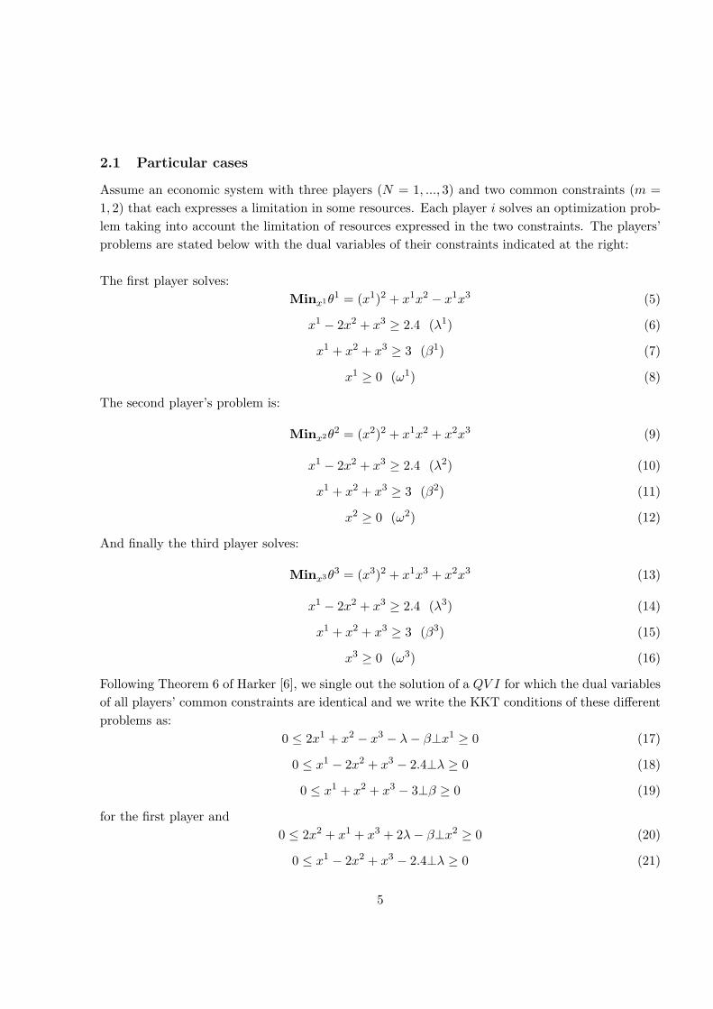
Assume an economic system with three players (N = 1, ..., 3) and two common constraints (m =1, 2) that each expresses a limitation in some resources. Each player i solves an optimization prob-lem taking into account the limitation of resources expressed in the two constraints. The players’problems are stated below with the dual variables of their constraints indicated at the right:

The first player solves:Minx1θ1 = (x1)2 + x1x2 − x1x3 (5)

x1 − 2x2 + x3 ≥ 2.4 (λ1) (6)

x1 + x2 + x3 ≥ 3 (β1) (7)

x1 ≥ 0 (ω1) (8)

The second player’s problem is:

Minx2θ2 = (x2)2 + x1x2 + x2x3 (9)

x1 − 2x2 + x3 ≥ 2.4 (λ2) (10)

x1 + x2 + x3 ≥ 3 (β2) (11)

x2 ≥ 0 (ω2) (12)

And finally the third player solves:

Minx3θ3 = (x3)2 + x1x3 + x2x3 (13)

x1 − 2x2 + x3 ≥ 2.4 (λ3) (14)

x1 + x2 + x3 ≥ 3 (β3) (15)

x3 ≥ 0 (ω3) (16)

Following Theorem 6 of Harker [6], we single out the solution of a QV I for which the dual variablesof all players’ common constraints are identical and we write the KKT conditions of these differentproblems as:

0 ≤ 2x1 + x2 − x3 − λ− β⊥x1 ≥ 0 (17)

0 ≤ x1 − 2x2 + x3 − 2.4⊥λ ≥ 0 (18)

0 ≤ x1 + x2 + x3 − 3⊥β ≥ 0 (19)

for the first player and0 ≤ 2x2 + x1 + x3 + 2λ− β⊥x2 ≥ 0 (20)

0 ≤ x1 − 2x2 + x3 − 2.4⊥λ ≥ 0 (21)

5

0 ≤ x1 + x2 + x3 − 3⊥β ≥ 0 (22)

for the second player. Finally for the third player:

0 ≤ 2x3 + x1 + x2 − λ− β⊥x3 ≥ 0 (23)

0 ≤ x1 − 2x2 + x3 − 2.4⊥λ ≥ 0 (24)

0 ≤ x1 + x2 + x3 − 3⊥β ≥ 0 (25)

The solution of this three players’ problem is x = [2.1, 0.2, 0.7]T . This makes the two constraintsbinding and λ and β amount to 0.167 and 3.533 respectively. We interpret this model as one wherea market allocates the common resources represented in the two constrains through a single pricesystem (one price for each constraint). We refer to this scenario as “case 1”.

Rosen’s ([12]) considers another solution of the QV I problem where the dual variables of theshared constraints are equal among all players up to a constant factor ri that depends on players,but not on the constraints. This is mathematically expressed as:

λi = λ/ri i = 1, 2, 3 (26)

βi = β/ri i = 1, 2, 3 (27)

Rosen refers to this solution as normalized equilibrium. The complementarity formulation of theproblem is as follows:

0 ≤ 2x1 + x2 − x3 − λ1 − β1⊥x1 ≥ 0 (28)

0 ≤ x1 − 2x2 + x3 − 2.4⊥λ1 ≥ 0 (29)

0 ≤ x1 + x2 + x3 − 3⊥β1 ≥ 0 (30)

for the first player, while that of the second player is:

0 ≤ 2x2 + x1 + x3 + 2λ2 − β2⊥x2 ≥ 0 (31)

0 ≤ x1 − 2x2 + x3 − 2.4⊥λ2 ≥ 0 (32)

0 ≤ x1 + x2 + x3 − 3⊥β2 ≥ 0 (33)

Finally that of the third player is stated as:

0 ≤ 2x3 + x1 + x2 − λ3 − β3⊥x3 ≥ 0 (34)

0 ≤ x1 − 2x2 + x3 − 2.4⊥λ3 ≥ 0 (35)

0 ≤ x1 + x2 + x3 − 3⊥β3 ≥ 0 (36)

Rosen’s normalized equilibrium is obtained when the dual variables of the shared constraintsare equal among all players up to a constant factor ri.

6

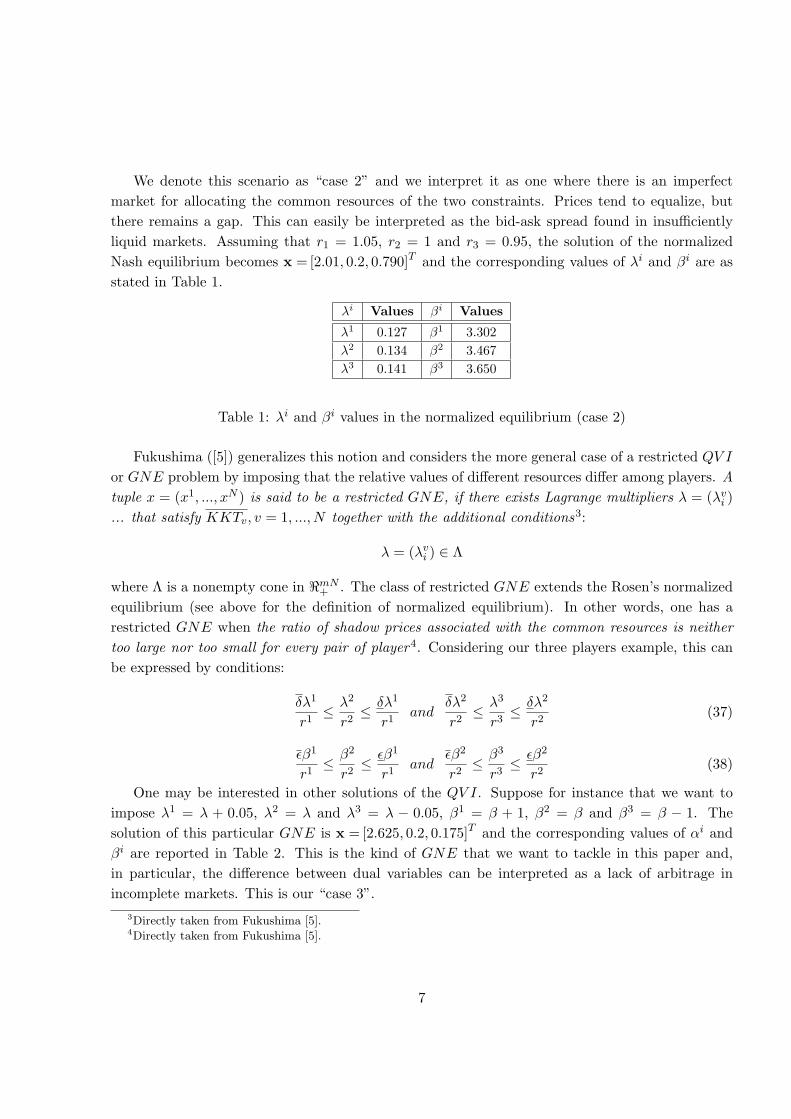
We denote this scenario as “case 2” and we interpret it as one where there is an imperfectmarket for allocating the common resources of the two constraints. Prices tend to equalize, butthere remains a gap. This can easily be interpreted as the bid-ask spread found in insufficientlyliquid markets. Assuming that r1 = 1.05, r2 = 1 and r3 = 0.95, the solution of the normalizedNash equilibrium becomes x = [2.01, 0.2, 0.790]T and the corresponding values of λi and βi are asstated in Table 1.

λi Values βi Values

λ1 0.127 β1 3.302λ2 0.134 β2 3.467λ3 0.141 β3 3.650

Table 1: λi and βi values in the normalized equilibrium (case 2)

Fukushima ([5]) generalizes this notion and considers the more general case of a restricted QV Ior GNE problem by imposing that the relative values of different resources differ among players. Atuple x = (x1, ..., xN ) is said to be a restricted GNE, if there exists Lagrange multipliers λ = (λvi )... that satisfy KKTv, v = 1, ..., N together with the additional conditions3:

λ = (λvi ) ∈ Λ

where Λ is a nonempty cone in <mN+ . The class of restricted GNE extends the Rosen’s normalizedequilibrium (see above for the definition of normalized equilibrium). In other words, one has arestricted GNE when the ratio of shadow prices associated with the common resources is neithertoo large nor too small for every pair of player4. Considering our three players example, this canbe expressed by conditions:

δλ1

r1≤ λ2

r2≤ δλ1

r1and

δλ2

r2≤ λ3

r3≤ δλ2

r2(37)

εβ1

r1≤ β2

r2≤ εβ1

r1and

εβ2

r2≤ β3

r3≤ εβ2

r2(38)

One may be interested in other solutions of the QV I. Suppose for instance that we want toimpose λ1 = λ + 0.05, λ2 = λ and λ3 = λ − 0.05, β1 = β + 1, β2 = β and β3 = β − 1. Thesolution of this particular GNE is x = [2.625, 0.2, 0.175]T and the corresponding values of αi andβi are reported in Table 2. This is the kind of GNE that we want to tackle in this paper and,in particular, the difference between dual variables can be interpreted as a lack of arbitrage inincomplete markets. This is our “case 3”.

3Directly taken from Fukushima [5].4Directly taken from Fukushima [5].

7

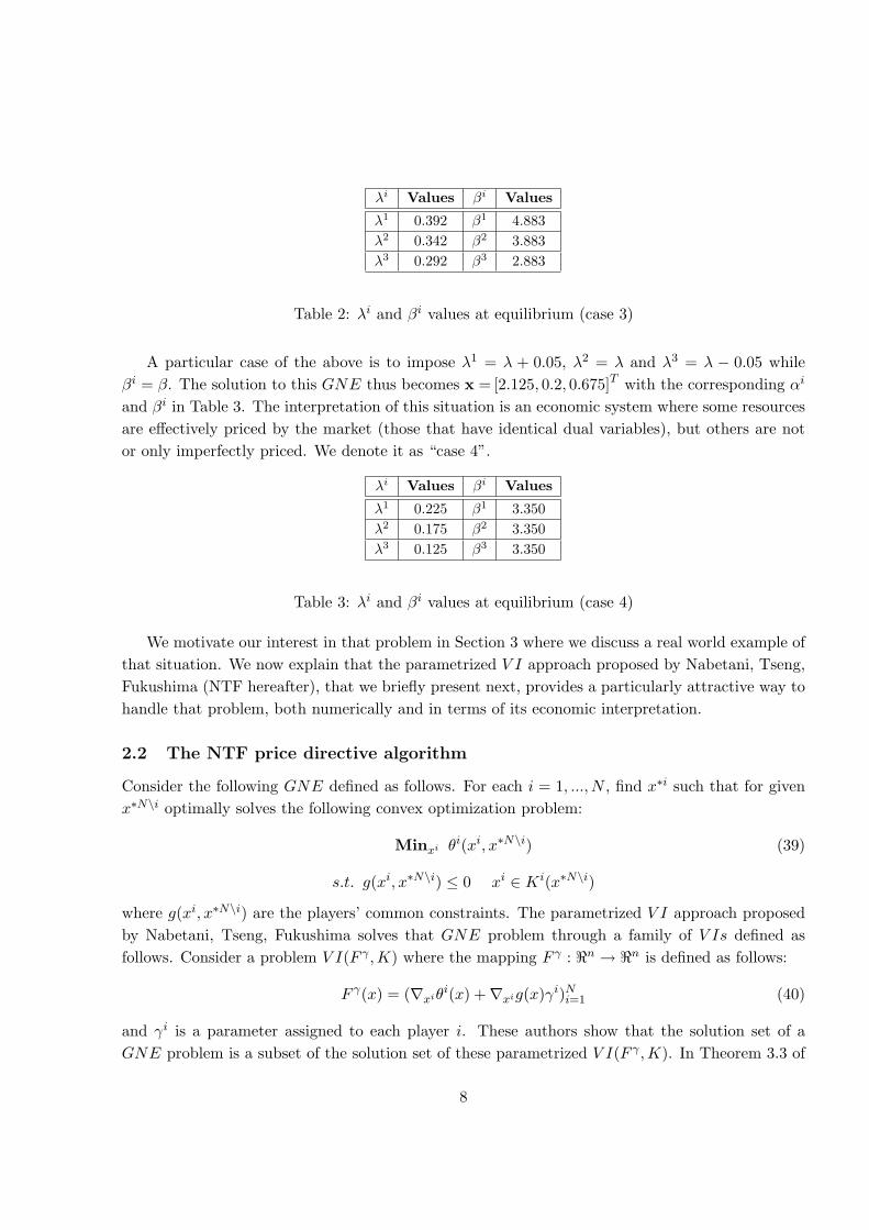
λi Values βi Values

λ1 0.392 β1 4.883λ2 0.342 β2 3.883λ3 0.292 β3 2.883

Table 2: λi and βi values at equilibrium (case 3)

A particular case of the above is to impose λ1 = λ + 0.05, λ2 = λ and λ3 = λ − 0.05 whileβi = β. The solution to this GNE thus becomes x = [2.125, 0.2, 0.675]T with the corresponding αi

and βi in Table 3. The interpretation of this situation is an economic system where some resourcesare effectively priced by the market (those that have identical dual variables), but others are notor only imperfectly priced. We denote it as “case 4”.

λi Values βi Values

λ1 0.225 β1 3.350λ2 0.175 β2 3.350λ3 0.125 β3 3.350

Table 3: λi and βi values at equilibrium (case 4)

We motivate our interest in that problem in Section 3 where we discuss a real world example ofthat situation. We now explain that the parametrized V I approach proposed by Nabetani, Tseng,Fukushima (NTF hereafter), that we briefly present next, provides a particularly attractive way tohandle that problem, both numerically and in terms of its economic interpretation.

2.2 The NTF price directive algorithm

Consider the following GNE defined as follows. For each i = 1, ..., N , find x∗i such that for givenx∗N\i optimally solves the following convex optimization problem:

Minxi θi(xi, x∗N\i) (39)

s.t. g(xi, x∗N\i) ≤ 0 xi ∈ Ki(x∗N\i)

where g(xi, x∗N\i) are the players’ common constraints. The parametrized V I approach proposedby Nabetani, Tseng, Fukushima solves that GNE problem through a family of V Is defined asfollows. Consider a problem V I(F γ ,K) where the mapping F γ : <n → <n is defined as follows:

F γ(x) = (∇xiθi(x) +∇xig(x)γi)Ni=1 (40)

and γi is a parameter assigned to each player i. These authors show that the solution set of aGNE problem is a subset of the solution set of these parametrized V I(F γ ,K). In Theorem 3.3 of

8

[7], they also give conditions for identifying when a solution of V I(F γ ,K) is effectively a GNE.Consider the KKT conditions for V I(F γ ,K):

0 ∈ [(∇xiθi(x) +∇xig(x)γi) +∇xig(x)π], i = 1, ..., N

0 ≤ π⊥g(x) ≥ 0, xi ∈ Xi, i = 1, ..., N

Theorem 3.3 says that for any γ ∈ <mN+ and any (x∗, π∗) ∈ <n × <m satisfying the KKTconditions indicated above, a sufficient condition for x∗ to be a GNE is that:

〈g(x∗), γi〉 = 0, i = 1, ..., N. (41)

If in addition a constraint qualification condition holds at x∗, then (41) is also a necessarycondition for x∗ to be a GNE. This algorithm can be easily adapted to the problem treated in thispaper.

The following section provides the economic intuition that motivates this problem. We firstpresent the problem in general terms and then adapt it to the particular situation that is treatedin Section 3.3.

3 Economic interpretation

3.1 A general production context

Nash equilibria are commonly used in economics to describe markets affected by market power. Incontrast, we concentrate in this paper on markets where all agents are price takers and hence thereis no market power. This was the context adopted by Debreu and Arrow and Debreu in [3] and [1]for introducing social equilibrium. Specifically we consider the following social equilibrium problemthat arises in production management. Consider the problem of decentralizing the activities of anorganization into different Business Units (BU) that is each evaluated on its own performance. Theinteractions between the business units are of two types. First, actions of one BU can influence thepayoff (performance index) of another BU . Second, all BUs share common constraints (resourceavailability or operations constraint) with the implication that the actions of one BU can changethe remaining resources available to the other BUs. Both types of interactions are known byeconomists as externalities. Negative externalities create inefficiencies; positive externalities createbenefits. While the organization can in principle achieve its best result by an overall optimization,it is believed that the centralization of operations required by this optimization decreases individualincentives to be efficient (moral hazard in economic parlance).

The decentralization process consists in assembling activities in BUs and organizing internalmarkets for shared resources. We explained that integrating all operations would maximize ef-ficiency where it is not for a degradation of individual incentives. In a similar way, efficiencyjustifies creating an internal market for all common resources or restrictions in the decentralizedorganisation (see the treatment of common constraints in Dantzig-Wolfe decomposition), except if,

9

following Williamson’s theory [14], externalizing transactions through these markets would increasecosts with respect to keeping them inside an integrated firm. There is thus a trade-off in decentral-ization between increasing individual incentives towards efficiency and incurring costs because ofloss of coordination. We justify the introduction of our problem as an instrument to measure theeconomic cost resulting from the loss of coordination in decentralized operations.

The economic problem can be analyzed in two stages. A first question is to group activitiesinto BUs, the other is to decide which resource or restriction to allocate through a market andwhich not. The first problem can be handled by testing different groupings of activities. Suppose,in order to treat the second question, that the decomposition of the overall organisation in BUs isdefined. The question then arises as to the creation of an internal market for common resources orrestrictions. The resources or constraints allocated through an internal market have a common pricecharged by all BUs. The other resources can be valued differently by the different BUs without anymarket reconciling these different valuations into a single price or opportunity cost. Inefficiencyarises from both improper grouping of activities and price differences that signal residual arbitragepossibilities. Assessing this inefficiency can then be done either by measuring the additional costincurred by the decentralized organization or by valuing the remaining arbitrage possibilities. TheNTF price directed algorithm provides a particularly attractive way to tackle that problem. Weapply these general ideas to the particular problem of counter-trading in restructured electricitysystems, that we describe after introducing a GNE formulation of the above discussion.

3.2 Formulation in terms of GNE

3.2.1 Problem statement

We formulate the above problem in the following abstract way. There are two BUs, each notedi = N,S (in order to use the same notation as in the rest of the paper). Each BU maximizes autility function U i(x) taking into account both common and individual constraints. Some of theconstraints are considered sufficiently important for organizing a common market. Others are seenas less important and hence left to informal arrangements.

Player N solves the following problem:

MaxxNUN (xN , xS) (42)

s.t.XN (xN ) = 0 (νN ) (43)

Y (xN , xS) = Y N (xN ) + Y S(xS) ≥ 0 (µN ) (44)

Z(xN , xS) = ZN (xN ) + ZS(xS) ≥ 0 (λN ) (45)

where the function UN and XN are respectively the utility and the own constraint of player N ; Yand Z are the common and separable constraints, Y denoting those for which a common market

10

has been put in place. The second player, labeled S (South), solves the following similar problem:

MaxxSUS(xN , xS) (46)

s.t.XS(xS) = 0 (νS) (47)

Y (xN , xS) = Y N (xN ) + Y S(xS) ≥ 0 (µS) (48)

Z(xN , xS) = ZN (xN ) + ZS(xS) ≥ 0 (λS) (49)

The combination of these two optimization problems constitutes a Generalized Nash Equilibriumproblem. Referring to the above interpretation we impose that the dual variables µN and µS areequal because they can be interpreted as a transfer price in the common market of constraints Y . Incontrast, λN and λS can be different because no internal market has been created for these commonconstraints. νN and νS refer to BUs’ own constraints and hence can be expected to be different.This is a particular Generalized Nash Equilibrium in the sense that some of the constraints arepriced by the market and hence their dual variables are equal for both players. But the marketis incomplete in the sense that it does not cover all common constraints and the dual variables ofthe uncovered constraints can be different. The theory of GNE tells us that there may be severalsolutions to this problem, implying that the outcome of the organization is intrinsically ambiguous.It is thus relevant to inquire whether these different outcomes can be far apart some of them beingquite inefficient compared to the outcome where all constraints would be priced by a completemarket. Conversely one may wonder whether there are cases where there is a single outcome (theQV I and the associated V I have identical solution sets).

We explore this question by applying the parametrized variational inequality approach describedby Nabetani, Tseng and Fukushima in [7] and construct the following parametrized model.

MaxxN,SUN (xN , xS) + US(xN , xS) + (ZN (xN ))γN + (ZS(xS))γS (50)

s.t.XN (xN ) = 0 (νN ) (51)

XS(xS) = 0 (νS) (52)

Y (xN , xS) = Y N (xN ) + Y S(xS) ≥ 0 (µ) (53)

Z(xN , xS) = ZN (xN ) + ZS(xS) ≥ 0 (λ) (54)

Changing the γ parameters leads to different Generalized Nash Equilibria provided that positive γare associated to a positive λ. There is only a single GNE if it is impossible to generate differentGNE by modifying the γ. Assuming adequate constraint qualification and the optimization prob-lem is feasible, this can only happen if the optimization problem is unbounded. This occurs if it

11

does not have any primal dual solution, a property that can be checked on the complementaritytheorem obtained from the KKT conditions of the optimization problem. These are stated as:

0 ≥ ∂xNUN (xN , xS)∂xN

+γN∂xNZ

N (xN )∂xN

+νN∂xNX

N (xN )∂xN

+µ∂xNY

N (xN )∂xN

+λ∂xNZ

N (xN )∂xN

⊥xN ≥ 0

0 ≥ ∂xSUS(xN , xS)∂xS

+ γS∂xSZ

S(xS)∂xS

+ νS∂xSX

S(xS)∂xS

+ µ∂xSY

S(xS)∂xS

+ λ∂xSZ

S(xS)∂xS

⊥xS ≥ 0

0 ≤ Y (xN , xS)⊥µ ≥ 0 (55)

0 ≤ Z(xN , xS)⊥λ ≥ 0 (56)

XN (xN ) = 0 (νN ) (57)

XS(xS) = 0 (νS) (58)

3.2.2 Assessing inefficiencies

The above model can be used to test the inefficiency of a particular organization. These arise fromtwo sources. One is in the delineation of the individual constraints of the BUs (the X constraints)when they result from an ex ante allocation of some common resources. The other source ofinefficiency is the absence of a common market for the resources that remain common. This isis expressed by the difference of valuation of these resources by the BU (the dual variables). Inall cases this implies a change of the utility function value of the BUs. It is this approach thatwe illustrate in the following application taken from the restructuring of the European electricitymarket.

3.3 Counter-trading in restructured electricity markets

The operations of the electricity system under the regulatory regime is the paradigm of the fullycentralized and optimized organisation of operations: all machines operating in the short run areunder the control of a single optimization problem. The underlying philosophy of the restructuringof the sector is that decentralising operations improve the incentive of individual agents (generators,traders, consumers) to be efficient, possibly at the cost of some loss of coordination of operations.The question is to find a good trade-off by gaining on incentives without loosing too much on coor-dination. We here consider a particular problem that arises in the European context of electricityrestructuring namely the organisation of counter-trading after the clearing of the energy market byPower Exchanges. A full description of the overall problem, namely the so called market coupling,would lead us too far away from the numerical objective of this paper and we therefore report abrief summary in Appendix A (see the companion paper [9] for more details). We here restrictourselves to the subproblem of counter-trading that we describe on the basis of a six node exampleinitially presented by Chao and Peck in [2].

12

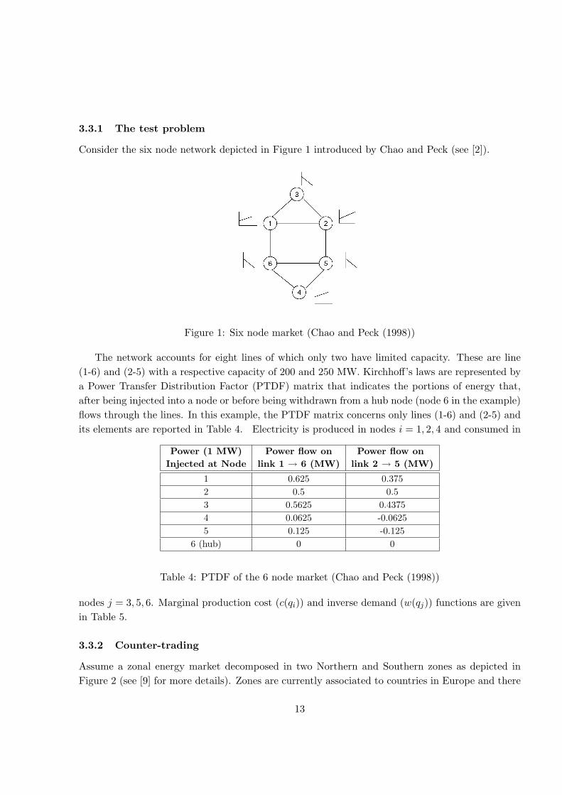
3.3.1 The test problem

Consider the six node network depicted in Figure 1 introduced by Chao and Peck (see [2]).

Figure 1: Six node market (Chao and Peck (1998))

The network accounts for eight lines of which only two have limited capacity. These are line(1-6) and (2-5) with a respective capacity of 200 and 250 MW. Kirchhoff’s laws are represented bya Power Transfer Distribution Factor (PTDF) matrix that indicates the portions of energy that,after being injected into a node or before being withdrawn from a hub node (node 6 in the example)flows through the lines. In this example, the PTDF matrix concerns only lines (1-6) and (2-5) andits elements are reported in Table 4. Electricity is produced in nodes i = 1, 2, 4 and consumed in

Power (1 MW) Power flow on Power flow onInjected at Node link 1 → 6 (MW) link 2 → 5 (MW)

1 0.625 0.3752 0.5 0.53 0.5625 0.43754 0.0625 -0.06255 0.125 -0.125

6 (hub) 0 0

Table 4: PTDF of the 6 node market (Chao and Peck (1998))

nodes j = 3, 5, 6. Marginal production cost (c(qi)) and inverse demand (w(qj)) functions are givenin Table 5.

3.3.2 Counter-trading

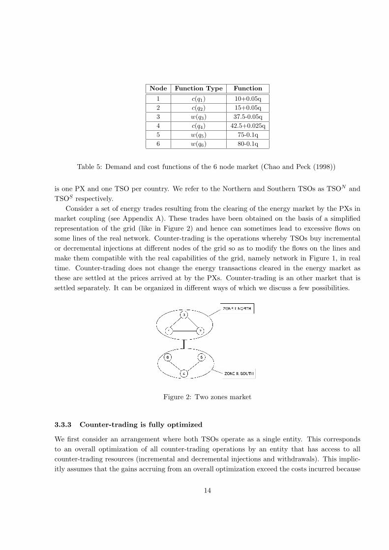
Assume a zonal energy market decomposed in two Northern and Southern zones as depicted inFigure 2 (see [9] for more details). Zones are currently associated to countries in Europe and there

13

Node Function Type Function

1 c(q1) 10+0.05q2 c(q2) 15+0.05q3 w(q3) 37.5-0.05q4 c(q4) 42.5+0.025q5 w(q5) 75-0.1q6 w(q6) 80-0.1q

Table 5: Demand and cost functions of the 6 node market (Chao and Peck (1998))

is one PX and one TSO per country. We refer to the Northern and Southern TSOs as TSON andTSOS respectively.

Consider a set of energy trades resulting from the clearing of the energy market by the PXs inmarket coupling (see Appendix A). These trades have been obtained on the basis of a simplifiedrepresentation of the grid (like in Figure 2) and hence can sometimes lead to excessive flows onsome lines of the real network. Counter-trading is the operations whereby TSOs buy incrementalor decremental injections at different nodes of the grid so as to modify the flows on the lines andmake them compatible with the real capabilities of the grid, namely network in Figure 1, in realtime. Counter-trading does not change the energy transactions cleared in the energy market asthese are settled at the prices arrived at by the PXs. Counter-trading is an other market that issettled separately. It can be organized in different ways of which we discuss a few possibilities.

Figure 2: Two zones market

3.3.3 Counter-trading is fully optimized

We first consider an arrangement where both TSOs operate as a single entity. This correspondsto an overall optimization of all counter-trading operations by an entity that has access to allcounter-trading resources (incremental and decremental injections and withdrawals). This implic-itly assumes that the gains accruing from an overall optimization exceed the costs incurred because

14

of the full harmonization and integrated control of the TSOs.

3.3.4 Counter-trading is decentralised

The second arrangement takes place when the two TSOs retain separate operations, but sharecommon constraints or resources. The capacities of the lines joining the Northern and Southernzones are common constraints used by both TSOs. They can be priced or not depending on whetherone introduces a market for transmission at the counter-trading level or not. We want to check theimpact of this pricing on the overall efficiency of counter-trading. Common economic sense indeedsuggests that the inception of a transmission capacity market increases efficiency. Counter-tradingresources at the generator or consumer levels are the other set of resources. They may be sharedby the two TSOs or not depending on the organisation. When shared, we assume, in compliancewith general non discrimination principles that both TSOs access them at the same price. Wedistinguish three extents of sharing counter-trading resources. A first situation is the one wherethere is effectively an internal market for counter-trading resources: both TSOs can have accessto all incremental and decremental injections in both zones. A second case is the one where thiscommon market exists, but is limited by quantitative constraints that are interpreted in terms ofsecurity: a TSO can only access part of the counter-trading resources of the other zone. The thirdsituation occurs when there is no common market for counter-trading resources. We also want toassess the impact of these different organisations on the overall efficiency of counter-trading. Wehere present the structure of the model and refer to a companion paper [9] for a broader analysisof numerical results.

3.3.5 Note on counter-trading costs

Re-dispatching costs interact with the PX’s bids and create a link between the market couplingand counter-trading problems. This is not discussed here, but illustrated in a companion paper(see [9]). For the sake of readability we report the average counter-trading cost α because it is easyto interpret and compare to the energy price. It is obtained by dividing the total counter-tradingcost (TCC) that varies with the model considered by the total generation (

∑i=1,2,4 qi). This is

defined as follows:α =

TCC∑i=1,2,4 qi

4 Modelling

The original NTF paper is stated in terms of variational inequality problems; our example dealswith variational inequality models that are integrable into optimization problems. We thereforeonly refer to optimization models, using the following nomenclature:

Sets

15

• l=(1-6);(2-5): Lines with limited capacity;

• n = 1, 2, 3, 4, 5, 6: Nodes

• i(n) = 1, 2, 4: Subet of production nodes;

• j(n) = 3, 5, 6: Subet of consumption nodes

Parameters

• PTDFl,n: Power Transfer Distribution Factor (PTDF) matrix of node n on line l;

• Fl: Limit of flow through lines l = (1− 6); (2− 5);

• qn: Power traded (bought or sold) in node n (MWh); these are determined in the marketcoupling problem and are taken as data in the counter-trading models.

Variables

• ∆qn: Counter-trading variables: Incremental or decremental quantities of electricity withrespect to qn (MWh).

We assume that all agents are price takers. They bid in both the day-ahead and counter-tradingmarkets. We do not separately model a balancing market taking care of deviations with respect today-ahead.

4.1 Counter-trading operations are optimized

Assume that TSON and TSOS buy incremental and decremental quantities of electricity ∆qn intheir domestic market (N = (1, 2, 3) and S = (4, 5, 6) respectively) and coordinate operations toremove congestion at the minimal counter-trading cost. This is stated in the optimization problem(59)-(65).

The global re-dispatching costs appears in the objective function (59). There are two classesof constraints. The first class involves both TSOs and includes the balance equations (60), (61)and the transmission capacity constraints (62) and (63). Conditions (60) and (61) impose thatthe sum of the incremental injections (∆qi=1,2,4) and withdrawals (∆qj=3,5,6) equals zero. Thisexpresses that the amount of energy cleared by the PX is not affected by counter-trading. Asalluded to before, this rule separates the trading of energy (the qn that remain unchanged) and thecounter-trading operations (the ∆qn variables that are counter-trading operations) in two differentmarkets. The dual variables λ±l associated with (62) and (63) respectively define the marginalvalues of the capacited lines (1-6) and (2-5) in the two flow directions. Because there is a singleoptimization problem for both TSOs, they see the same value for the congested lines. In the secondclass, we group constraints (64)-(65) that are specific to the geographic zone covered by each TSO.

16

The non-negativity constraints (64) state that the quantities of electricity demanded and producedin the Northern zone plus the incremental and decremental injections of the TSON have to benon-negative. An identical reasoning applies in condition (65) for the zone covered by TSOS .

Min∆qn

∑i=1,2,4

∫ qi+∆qi

qi

ci(ξ)dξ −∑

j=3,5,6

∫ qj+∆qj

qj

wj(ξ)dξ (59)

s.t. ∑i=1,2,4

∆qi +∑

j=3,5,6

∆qj = 0 (µ1) (60)

∑i=1,2,4

∆qi −∑

j=3,5,6

∆qj = 0 (µ2) (61)

F l − [∑

i=1,2,4

PTDFi,l(qi + ∆qi)−∑

j=3,5,6

PTDFj,l(qj + ∆qj)] ≥ 0 (λ+l ) (62)

F l + [∑

i=1,2,4

PTDFi,l(qi + ∆qi)−∑

j=3,5,6

PTDFj,l(qj + ∆qj)] ≥ 0 (λ−l ) (63)

qn + ∆qn ≥ 0 n = 1, 2, 3 (νNn ) (64)

qn + ∆qn ≥ 0 n = 4, 5, 6 (νSn ) (65)

Problem (59)-(65) is strictly convex and admits a unique solution. This model provides thebenchmark for evaluating other organizations of counter-trading. Finally, the average re-dispatchingcosts α is computed by dividing the objective function (59) by

∑i=1,2,4 qi.

4.2 Decentralized counter-trading Model 1: TSON and TSOS have full access

to all re-dispatching resources

TSON and TSOS no longer cooperate for removing network congestion, but still have full access toall counter-trading resources of the system. This means that a TSO can buy and sell incrementaland decremental injections and withdrawals in the control area of the other TSO (e.g. TSON canalso counter-trade in the Southern zone and vice versa). This situation can be interpreted as thecreation of an internal market of counter-trading resources. Denoting the counter-trading variablesof the Northern and Southern TSOs respectively as ∆qNn=1,...,6 and ∆qSn=1,...,6, the following presentsthe problem of TSON , the problem of TSOS is similar and given in Appendix C.

4.2.1 Problem of TSON

TSON solves the optimization problem (66)-(71). It minimizes its re-dispatching costs (66) takinginto account its balance constraints (67) and (68) (each TSO must remain in balance) and thecounter-trading actions of the other TSO. These actions appear in the transmission constraints(69)-(70), and the overall non-negativity constraint (71) on generation and consumption. Note

17

that constraints (67) and (68) are specific to the single Northen TSO while (69)-(70), and (71)involve both TSOs.

Min∆qNn

∑i=1,2,4

∫ qi+∆qSi +∆qNi

qi+∆qSi

ci(ξ)dξ −∑

j=3,5,6

∫ qj+∆qSj +∆qNj

qj+∆qSj

wj(ξ)dξ (66)

s.t. ∑i=1,2,4

∆qNi +∑

j=3,5,6

∆qNj = 0 (µN,1) (67)

∑j=3,5,6

∆qNj −∑

i=1,2,4

∆qNi = 0 (µN,2) (68)

F l − [∑

i=1,2,4

PTDFi,l(qi + ∆qNi + ∆qSi )−∑

j=3,5,6

PTDFj,l(qj + ∆qSj + ∆qNj )] ≥ 0 (λN,+l ) (69)

F l + [∑

i=1,2,4

PTDFi,l(qi + ∆qNi + ∆qSi )−∑

j=3,5,6

PTDFj,l(qj + ∆qSj + ∆qNj )] ≥ 0 (λN,−l ) (70)

where l = (1− 6), (2− 5)qn + ∆qNn + ∆qSn ≥ 0 ∀n (νNn ) (71)

4.2.2 An efficient Generalized Nash Equilibrium

The combination of both TSOs’ problems suggests a Generalized Nash Equilibrium model that wewant to interpret in terms of markets for counter-trading resources and transmission capacities.

A first step towards the creation of an internal market of counter-trading resources is that bothTSON and TSOS have access to the same incremental and decremental injections and withdrawals.This is stated in the constraints (67)-(68) of the TSON and (114)-(115) of the TSOS ’s problems(see Appendix C). The intended effect is that this access should be at the same price for both TSOs.This remains to be proved. One may also wish to create a market of transmission capacities. Thisis expressed by the constraints imposed on the dual variables of constraints (71) for TSON and theanalogous constraint for TSOS . Imposing the equality of these dual variables amounts to assumea market of transmission capacities as both TSOs see the same price for transmission resources. Incontrast, there is no market for line capacity in the counter-trading system if the dual variables of(69)-(70) for TSON and (116)-(117) for TSOS can be different.

The two assumptions of transmission market can be easily cast in the NTF parametrizedoptimization problem (72)-(80) (a parametrized V I problem in general). The objective function(72) combines the actions of both TSOs and also includes the parameters5 γN,S,± that perturb

5The apeces N,S of the parameters γN,S,± indicate “North” and “South”; while the sign “+” and “-” indicate the

flow directions. The positive direction is from the Northern to the Southern zone; the negative direction is from the

Southern to the Northern zone.

18

the dual variables λ+l and λ−l associated with the common transmission constraints (77) and (78).

Setting the γN,S,± to zero implies equal dual variables of the transmission constraints and hencea transmission market. Setting them at different values represents the case where there is notransmission market. While (77) and (78) are common to TSON and TSOS , the balance conditions(73), (74), (75) and (76) apply to each individual TSO. Conditions (73)-(74) are identical to (67)-(68) and refer to TSON , while (75) and (76) regard TSOS (compare (114) and (115) in AppendixC).

Min∆qN,S

n

∑i=1,2,4

∫ qi+∆qNi +∆qSi

qi

ci(ξ)dξ −∑

j=3,5,6

∫ qj+∆qNj +∆qSj

qj

wj(ξ)dξ+ (72)

+(γN,+l − γN,−l ) · (∑

i=1,2,4;l

PTDFi,l ·∆qNi −∑

j=3,5,6;l

PTDFj,l ·∆qNj )

+(γS,+l − γS,−l ) · (∑

i=1,2,4;l

PTDFi,l ·∆qSi −∑

j=3,5,6;l

PTDFj,l ·∆qSj )

s.t. ∑i=1,2,4

∆qNi +∑

j=3,5,6

∆qNj = 0 (µN,1) (73)

∑j=3,5,6

∆qNj −∑

i=1,2,4

∆qNi = 0 (µN,2) (74)

∑i=1,2,4

∆qSi +∑

j=3,5,6

∆qSj = 0 (µS,1) (75)

∑j=3,5,6

∆qSj −∑

i=1,2,4

∆qSi = 0 (µS,2) (76)

F l − [∑

i=1,2,4

PTDFi,l(qi + ∆qNi + ∆qSi )−∑

j=3,5,6

PTDFj,l(qj + ∆qNj + ∆qSj )] ≥ 0 (λ+l ) (77)

F l + [∑

i=1,2,4

PTDFi,l(qi + ∆qNi + ∆qSi )−∑

j=3,5,6

PTDFj,l(qj + ∆qNj + ∆qSj )] ≥ 0 (λ−l ) (78)

where l = (1− 6), (2− 5)

qn + ∆qNn + ∆qSn ≥ 0 ∀n (νNn ) (79)

qn + ∆qNn + ∆qSn ≥ 0 ∀n (νSn ) (80)

While the above formulation accounts for the fact that both TSOs have access to the samecounter-trading resources (balance conditions (73), (74), (75) and (76)), it does not imply yet thatthey see the same prices for them as one would expect in an internal market of these resources.This relation is established in the following propositions.

19

Proposition 1 Denote transmission constraints (77) and (78) respectively as g+l and g−l . Suppose

that⟨g+l (x∗), γN/S,+l

⟩= 0 and

⟨g−l (x∗), γN/S,−l

⟩= 0. The solution of problem (72)-(80) is a GNE

if and only if γN,+l = γS,+l and γN,−l = γS,−l .

Proof 1 See Appendix E. �

The implication of this proposition is that a GNE solution of this problem, if it exists, hasidentical dual variables for the transmission constraints. This amounts to creating a market oftransmission resources. It also implies a single price for counter-trading resources thereby com-pleting the proof that we did create an internal market of these resources. This is stated in thefollowing proposition.

Proposition 2 The solution of the GNE problem (72)-(80), if it exists satisfies λN,±l = λS,±l ;µN,1 = µS,1 and µN,2 = µS,2 .

Proof 2 See Appendix F. �

The interpretation of this second proposition is twofold. From a mathematical point of viewit expresses that the solution set of the QV I associated to this GNE problem is identical to thesolution set of the related V I problem. This identifies a class of problems for which the solutions setsof the QV I and V I are identical. The economic interpretation of that problem is that introducinga common access to counter-trading resources, implicitly implies the existence of a market fortransmission resources and an internal (non discriminatory) market of counter-trading resources.In other words, an internal market of counter-trading resources “completes” the market.

The next implication is an expected result. A complete market is efficient; the outcome shouldbe identical to the one of the full optimization of counter-trading. This also proves that the solutionof the GNE (72)-(80), if it exists, is unique. This is expressed in the following corollaries.

Corollary 1 Suppose the solution to coordinated counter-trading problem (59)-(65) exists. Then,the solution of the GNE problem (72)-(80) exists and coincides with that of the coordinated counter-trading problem (59)-(65).

Proof 3 See Appendix G. �

Corollary 2 The solution of the GNE problem (72)-(80) is unique.

Proof 4 Since the solution to problem (59)-(65) is unique (see Section 4.1), thanks to Corollary1, we can immediately conclude that the solution to problem (72)-(80) is unique too. �

20

4.3 Decentralized counter-trading Model 2: TSON and TSOS have limited ac-

cess to part of the counter-trading resources

4.3.1 A partial market of counter-trading resources

The model presented in Section 4.2 assumes that both TSOs have full access to all re-dispatchingresources. We depart from this assumption here and model the case where both TSON and TSOS

have a limited access to the counter-trading resources located outside of their control area. Thismeans that the Northern TSO’s purchase of Southern counter-trading resources is limited andconversely. The optimization problems of each TSO are immediately derived from those in Section4.2 by adding upper and lower constraints on the variables defining re-dispatching in the zone notdirectly controlled by this TSO. We do not report these individual optimization problems here,but directly present the model in the Nabetani, Tseng and Fukushima’s form. The additionalconstraints (86) and (87) impose the upper and lower bounds on the actions of two TSOs in thejurisdiction that is not under their direct control. Condition (86) limits the TSON ’s purchase ofSouthern counter-trading resources and condition (87) does the same for TSOS in the Northernzone. This arrangement is likely to be more realistic (“pragmatic” in usual parlance) than theabove creation of an internal market: TSOs that are not integrated will probably insists on keepingresources under their sole control. We shall see that giving up the internal market of counter-trading resources can have dramatic consequences. We discuss these consequences in principle inthis paper together with some numerical results. We further elaborate on these numerical resultsin our companion paper (see [9]).

4.3.2 Inefficient Generalized Nash Equilibrium

Let ∆qNn and ∆qSn be respectively the bounds (in absolute value) imposed on TSOs resorting tooutside resources. The other conditions and constraints are as in Section 4.2. The NTS problem isstated as follows:

Min∆qN,S

n

∑i=1,2,4

∫ qi+∆qSi +∆qNi

qi

ci(ξ)dξ −∑

j=3,5,6

∫ qj+∆qSj +∆qNj

qj

wj(ξ)dξ+ (81)

+(γN,+l − γN,−l ) · (∑

i=1,2,4;l

PTDFi,l ·∆qNi −∑

j=3,5,6;l

PTDFj,l ·∆qNj )

+(γS,+l − γS,−l ) · (∑

i=1,2,4;l

PTDFi,l ·∆qSi −∑

j=3,5,6;l

PTDFj,l ·∆qSj )

s.t. ∑i=1,2,4

∆qNi +∑

j=3,5,6

∆qNj = 0 (µN,1) (82)

∑j=3,5,6

∆qNj −∑

i=1,2,4

∆qNi = 0 (µN,2) (83)

21

∑i=1,2,4

∆qSi +∑

j=3,5,6

∆qSj = 0 (µS,1) (84)

∑j=3,5,6

∆qSj −∑

i=1,2,4

∆qSi = 0 (µS,2) (85)

−∆qNn ≤ ∆qNn ≤ ∆qNn n = 4, 5, 6 (ηN,±n ) (86)

−∆qSn ≤ ∆qSn ≤ ∆qSn n = 1, 2, 3 (ηS,±n ) (87)

F l − [∑

i=1,2,4

PTDFi,l(qi + ∆qNi + ∆qSi )−∑

j=3,5,6

PTDFj,l(qj + ∆qSj + ∆qNj )] ≥ 0 (λ+l ) (88)

F l + [∑

i=1,2,4

PTDFi,l(qi + ∆qNi + ∆qSi )−∑

j=3,5,6

PTDFj,l(qj + ∆qSj + ∆qNj )] ≥ 0 (λ−l ) (89)

where l = (1− 6), (2− 5)

qn + ∆qNn + ∆qSn ≥ 0 ∀n (νNn ) (90)

qn + ∆qNn + ∆qSn ≥ 0 ∀n (νSn ) (91)

The following proposition is a preliminary; it gives the condition for the existence of GeneralizedNash Equilibrium and is a direct application of the NTF results.

Proposition 3 Denote transmission constraints (88) and (89) respectively by g+l and g−l . Suppose

that⟨g+l (x∗), γN/S,+l

⟩= 0 and

⟨g−l (x∗), γN/S,−l

⟩= 0. If the solution to problem (81)-(91) exists,

it is a GNE.

Proof 5 The proof is a direct application of NTF’s Theorem 3.3 (see [7]). �

In contrast with the case of the internal market of counter-trading resources, the outcome of themarket is here ambiguous: there may be several GNEs and they may differ in terms of efficiency.We first state that we fall back on the case of the internal market of counter-trading resources(decentralized Model 1) if none of the quantitative restrictions of cross zonal resources is binding.This means that the resources remaining of the exclusive control of the zonal TSO are not tooimportant.

Proposition 4 Denote transmission constraints (88) and (89) respectively as to g+l and g−l . Sup-

pose that⟨g+l (x∗), γN/S,+l

⟩= 0 and

⟨g−l (x∗), γN/S,−l

⟩= 0. If the solution to problem (81)-(91)

exists and no cross zonal counter-trading resource is binding, then γN,+/−l = γ

S,+/−l and the GNE

is unique and identical to the solution of the optimized counter-trading.

Proof 6 Apply the proof of Appendix E after noting that the KKT conditions of problem (72)-(80) are identical to those of problem (81)-(91) when cross zonal quantitative restrictions are notbinding. �

22

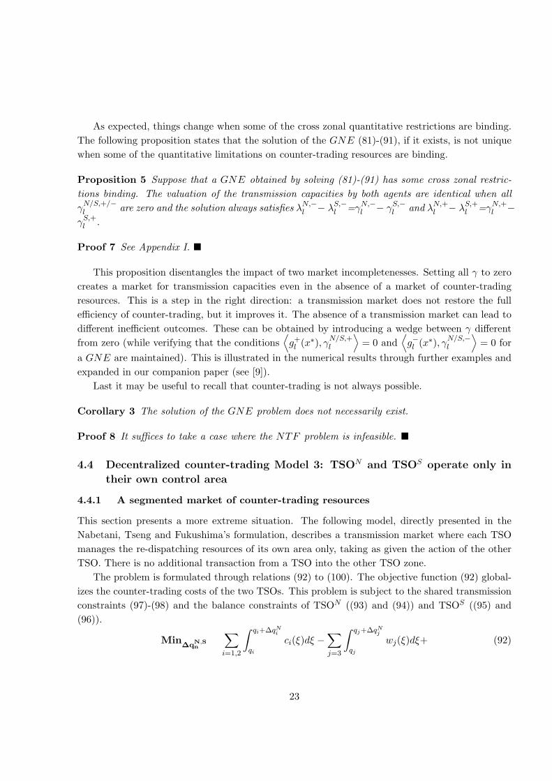
As expected, things change when some of the cross zonal quantitative restrictions are binding.The following proposition states that the solution of the GNE (81)-(91), if it exists, is not uniquewhen some of the quantitative limitations on counter-trading resources are binding.

Proposition 5 Suppose that a GNE obtained by solving (81)-(91) has some cross zonal restric-tions binding. The valuation of the transmission capacities by both agents are identical when allγN/S,+/−l are zero and the solution always satisfies λN,−l − λS,−l =γN,−l − γS,−l and λN,+l − λS,+l =γN,+l −γS,+l .

Proof 7 See Appendix I. �

This proposition disentangles the impact of two market incompletenesses. Setting all γ to zerocreates a market for transmission capacities even in the absence of a market of counter-tradingresources. This is a step in the right direction: a transmission market does not restore the fullefficiency of counter-trading, but it improves it. The absence of a transmission market can lead todifferent inefficient outcomes. These can be obtained by introducing a wedge between γ differentfrom zero (while verifying that the conditions

⟨g+l (x∗), γN/S,+l

⟩= 0 and

⟨g−l (x∗), γN/S,−l

⟩= 0 for

a GNE are maintained). This is illustrated in the numerical results through further examples andexpanded in our companion paper (see [9]).

Last it may be useful to recall that counter-trading is not always possible.

Corollary 3 The solution of the GNE problem does not necessarily exist.

Proof 8 It suffices to take a case where the NTF problem is infeasible. �

4.4 Decentralized counter-trading Model 3: TSON and TSOS operate only in

their own control area

4.4.1 A segmented market of counter-trading resources

This section presents a more extreme situation. The following model, directly presented in theNabetani, Tseng and Fukushima’s formulation, describes a transmission market where each TSOmanages the re-dispatching resources of its own area only, taking as given the action of the otherTSO. There is no additional transaction from a TSO into the other TSO zone.

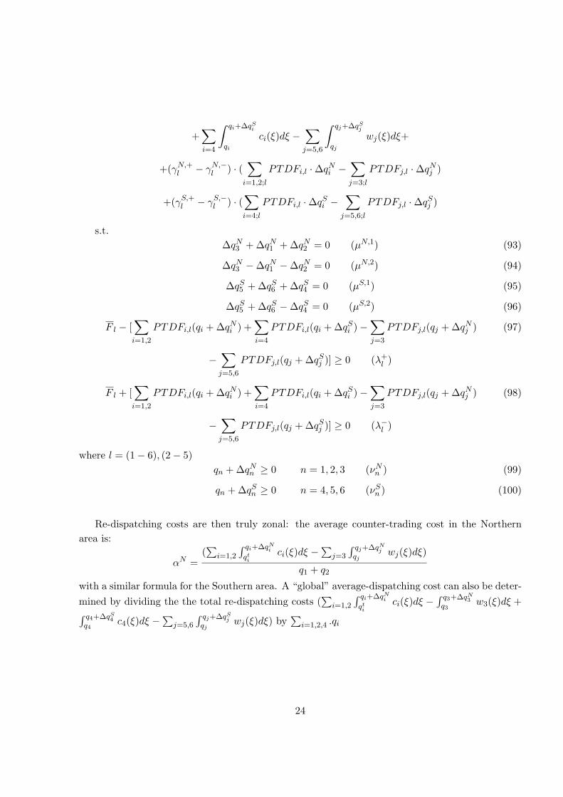
The problem is formulated through relations (92) to (100). The objective function (92) global-izes the counter-trading costs of the two TSOs. This problem is subject to the shared transmissionconstraints (97)-(98) and the balance constraints of TSON ((93) and (94)) and TSOS ((95) and(96)).

Min∆qN,S

n

∑i=1,2

∫ qi+∆qNi

qi

ci(ξ)dξ −∑j=3

∫ qj+∆qNj

qj

wj(ξ)dξ+ (92)

23

+∑i=4

∫ qi+∆qSi

qi

ci(ξ)dξ −∑j=5,6

∫ qj+∆qSj

qj

wj(ξ)dξ+

+(γN,+l − γN,−l ) · (∑i=1,2;l

PTDFi,l ·∆qNi −∑j=3;l

PTDFj,l ·∆qNj )

+(γS,+l − γS,−l ) · (∑i=4;l

PTDFi,l ·∆qSi −∑j=5,6;l

PTDFj,l ·∆qSj )

s.t.∆qN3 + ∆qN1 + ∆qN2 = 0 (µN,1) (93)

∆qN3 −∆qN1 −∆qN2 = 0 (µN,2) (94)

∆qS5 + ∆qS6 + ∆qS4 = 0 (µS,1) (95)

∆qS5 + ∆qS6 −∆qS4 = 0 (µS,2) (96)

F l − [∑i=1,2

PTDFi,l(qi + ∆qNi ) +∑i=4

PTDFi,l(qi + ∆qSi )−∑j=3

PTDFj,l(qj + ∆qNj ) (97)

−∑j=5,6

PTDFj,l(qj + ∆qSj )] ≥ 0 (λ+l )

F l + [∑i=1,2

PTDFi,l(qi + ∆qNi ) +∑i=4

PTDFi,l(qi + ∆qSi )−∑j=3

PTDFj,l(qj + ∆qNj ) (98)

−∑j=5,6

PTDFj,l(qj + ∆qSj )] ≥ 0 (λ−l )

where l = (1− 6), (2− 5)qn + ∆qNn ≥ 0 n = 1, 2, 3 (νNn ) (99)

qn + ∆qSn ≥ 0 n = 4, 5, 6 (νSn ) (100)

Re-dispatching costs are then truly zonal: the average counter-trading cost in the Northernarea is:

αN =(∑

i=1,2

∫ qi+∆qNiqti

ci(ξ)dξ −∑

j=3

∫ qj+∆qNjqj

wj(ξ)dξ)

q1 + q2

with a similar formula for the Southern area. A “global” average-dispatching cost can also be deter-mined by dividing the the total re-dispatching costs (

∑i=1,2

∫ qi+∆qNiqti

ci(ξ)dξ −∫ q3+∆qN3q3

w3(ξ)dξ +∫ q4+∆qS4q4

c4(ξ)dξ −∑

j=5,6

∫ qj+∆qSjqj

wj(ξ)dξ) by∑

i=1,2,4 .qi

24

4.4.2 Further inefficient Generalized Nash Equilibrium

The following propositions are particular cases of those obtained in the preceding section. The firststatement again directly obtains from NTF’s results: it simply states the conditions under whichthe solution of this problem is a GNE.

Proposition 6 Denote transmission constraints (97) and (98) respectively by g+l and g−l . Suppose

that⟨g+l (x∗), γN/S,+l

⟩= 0 and

⟨g−l (x∗), γN/S,−l

⟩= 0. If the solution to problem (92) to (100)

exists, it is a GNE.

Proof 9 The proof is a direct application of NTF’s Theorem 3.3 (see [7]). �

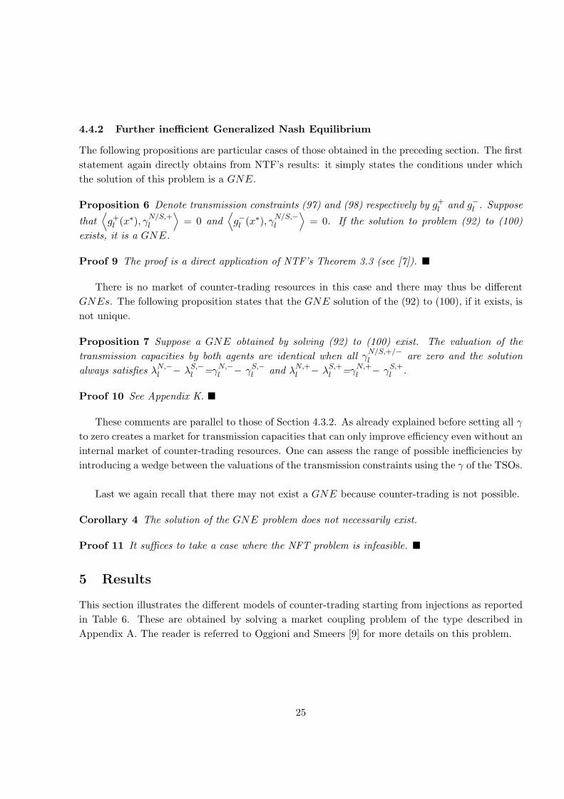
There is no market of counter-trading resources in this case and there may thus be differentGNEs. The following proposition states that the GNE solution of the (92) to (100), if it exists, isnot unique.

Proposition 7 Suppose a GNE obtained by solving (92) to (100) exist. The valuation of thetransmission capacities by both agents are identical when all γN/S,+/−l are zero and the solutionalways satisfies λN,−l − λS,−l =γN,−l − γS,−l and λN,+l − λS,+l =γN,+l − γS,+l .

Proof 10 See Appendix K. �

These comments are parallel to those of Section 4.3.2. As already explained before setting all γto zero creates a market for transmission capacities that can only improve efficiency even without aninternal market of counter-trading resources. One can assess the range of possible inefficiencies byintroducing a wedge between the valuations of the transmission constraints using the γ of the TSOs.

Last we again recall that there may not exist a GNE because counter-trading is not possible.

Corollary 4 The solution of the GNE problem does not necessarily exist.

Proof 11 It suffices to take a case where the NFT problem is infeasible. �

5 Results

This section illustrates the different models of counter-trading starting from injections as reportedin Table 6. These are obtained by solving a market coupling problem of the type described inAppendix A. The reader is referred to Oggioni and Smeers [9] for more details on this problem.

25

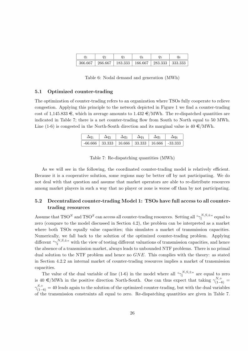
q1 q2 q3 q4 q5 q6

366.667 266.667 183.333 166.667 283.333 333.333

Table 6: Nodal demand and generation (MWh)

5.1 Optimized counter-trading

The optimization of counter-trading refers to an organization where TSOs fully cooperate to relievecongestion. Applying this principle to the network depicted in Figure 1 we find a counter-tradingcost of 1,145.833 e, which in average amounts to 1.432 e/MWh. The re-dispatched quantities areindicated in Table 7; there is a net counter-trading flow from South to North equal to 50 MWh.Line (1-6) is congested in the North-South direction and its marginal value is 40 e/MWh.

∆q1 ∆q2 ∆q3 ∆q4 ∆q5 ∆q6-66.666 33.333 16.666 33.333 16.666 -33.333

Table 7: Re-dispatching quantities (MWh)

As we will see in the following, the coordinated counter-trading model is relatively efficient.Because it is a cooperative solution, some regions may be better off by not participating. We donot deal with that question and assume that market operators are able to re-distribute resourcesamong market players in such a way that no player or zone is worse off than by not participating.

5.2 Decentralized counter-trading Model 1: TSOs have full access to all counter-

trading resources

Assume that TSON and TSOS can access all counter-trading resources. Setting all “γN,S,±l ” equal tozero (compare to the model discussed in Section 4.2), the problem can be interpreted as a marketwhere both TSOs equally value capacities; this simulates a market of transmission capacities.Numerically, we fall back to the solution of the optimized counter-trading problem. Applyingdifferent “γN,S,±l ” with the view of testing different valuations of transmission capacities, and hencethe absence of a transmission market, always leads to unbounded NTF problems. There is no primaldual solution to the NTF problem and hence no GNE. This complies with the theory: as statedin Section 4.2.2 an internal market of counter-trading resources implies a market of transmissioncapacities.

The value of the dual variable of line (1-6) in the model where all “γN,S,±l ” are equal to zerois 40 e/MWh in the positive direction North-South. One can thus expect that taking γN,+(1−6) =

γS,+(1−6) = 40 leads again to the solution of the optimized counter-trading, but with the dual variablesof the transmission constraints all equal to zero. Re-dispatching quantities are given in Table 7.

26

The sole important figure is the total (the sum over the two TSOs) re-dispatching; the allocationof this total between the two agents is arbitrary.

5.3 Imperfectly coordinated counter-trading Model 2: TSON and TSOS have

limited access to part of the counter-trading resources

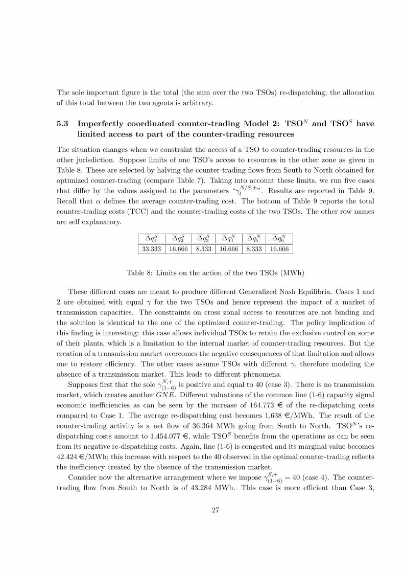
The situation changes when we constraint the access of a TSO to counter-trading resources in theother jurisdiction. Suppose limits of one TSO’s access to resources in the other zone as given inTable 8. These are selected by halving the counter-trading flows from South to North obtained foroptimized counter-trading (compare Table 7). Taking into account these limits, we run five casesthat differ by the values assigned to the parameters “γN/S,±l ”. Results are reported in Table 9.Recall that α defines the average counter-trading cost. The bottom of Table 9 reports the totalcounter-trading costs (TCC) and the counter-trading costs of the two TSOs. The other row namesare self explanatory.

∆qS1 ∆qS

2 ∆qS3 ∆qN

4 ∆qN5 ∆qN

6

33.333 16.666 8.333 16.666 8.333 16.666

Table 8: Limits on the action of the two TSOs (MWh)

These different cases are meant to produce different Generalized Nash Equilibria. Cases 1 and2 are obtained with equal γ for the two TSOs and hence represent the impact of a market oftransmission capacities. The constraints on cross zonal access to resources are not binding andthe solution is identical to the one of the optimized counter-trading. The policy implication ofthis finding is interesting: this case allows individual TSOs to retain the exclusive control on someof their plants, which is a limitation to the internal market of counter-trading resources. But thecreation of a transmission market overcomes the negative consequences of that limitation and allowsone to restore efficiency. The other cases assume TSOs with different γ, therefore modeling theabsence of a transmission market. This leads to different phenomena.

Supposes first that the sole γN,+(1−6) is positive and equal to 40 (case 3). There is no transmissionmarket, which creates another GNE. Different valuations of the common line (1-6) capacity signaleconomic inefficiencies as can be seen by the increase of 164.773 e of the re-dispatching costscompared to Case 1. The average re-dispatching cost becomes 1.638 e/MWh. The result of thecounter-trading activity is a net flow of 36.364 MWh going from South to North. TSON ’s re-dispatching costs amount to 1,454.077 e, while TSOS benefits from the operations as can be seenfrom its negative re-dispatching costs. Again, line (1-6) is congested and its marginal value becomes42.424 e/MWh; this increase with respect to the 40 observed in the optimal counter-trading reflectsthe inefficiency created by the absence of the transmission market.

Consider now the alternative arrangement where we impose γS,+(1−6) = 40 (case 4). The counter-trading flow from South to North is of 43.284 MWh. This case is more efficient than Case 3,

27

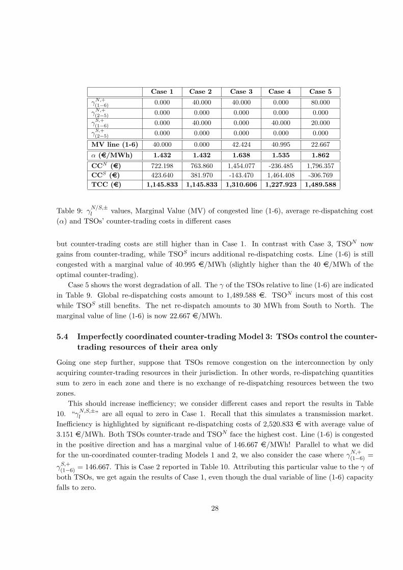
Case 1 Case 2 Case 3 Case 4 Case 5

γN,+(1−6) 0.000 40.000 40.000 0.000 80.000γN,+(2−5) 0.000 0.000 0.000 0.000 0.000γS,+(1−6) 0.000 40.000 0.000 40.000 20.000γS,+(2−5) 0.000 0.000 0.000 0.000 0.000

MV line (1-6) 40.000 0.000 42.424 40.995 22.667

α (e/MWh) 1.432 1.432 1.638 1.535 1.862

CCN (e) 722.198 763.860 1,454.077 -236.485 1,796.357CCS (e) 423.640 381.970 -143.470 1,464.408 -306.769TCC (e) 1,145.833 1,145.833 1,310.606 1,227.923 1,489.588

Table 9: γN/S,±l values, Marginal Value (MV) of congested line (1-6), average re-dispatching cost(α) and TSOs’ counter-trading costs in different cases

but counter-trading costs are still higher than in Case 1. In contrast with Case 3, TSON nowgains from counter-trading, while TSOS incurs additional re-dispatching costs. Line (1-6) is stillcongested with a marginal value of 40.995 e/MWh (slightly higher than the 40 e/MWh of theoptimal counter-trading).

Case 5 shows the worst degradation of all. The γ of the TSOs relative to line (1-6) are indicatedin Table 9. Global re-dispatching costs amount to 1,489.588 e. TSON incurs most of this costwhile TSOS still benefits. The net re-dispatch amounts to 30 MWh from South to North. Themarginal value of line (1-6) is now 22.667 e/MWh.

5.4 Imperfectly coordinated counter-trading Model 3: TSOs control the counter-

trading resources of their area only

Going one step further, suppose that TSOs remove congestion on the interconnection by onlyacquiring counter-trading resources in their jurisdiction. In other words, re-dispatching quantitiessum to zero in each zone and there is no exchange of re-dispatching resources between the twozones.

This should increase inefficiency; we consider different cases and report the results in Table10. “γN,S,±l ” are all equal to zero in Case 1. Recall that this simulates a transmission market.Inefficiency is highlighted by significant re-dispatching costs of 2,520.833 e with average value of3.151 e/MWh. Both TSOs counter-trade and TSON face the highest cost. Line (1-6) is congestedin the positive direction and has a marginal value of 146.667 e/MWh! Parallel to what we didfor the un-coordinated counter-trading Models 1 and 2, we also consider the case where γN,+(1−6) =

γS,+(1−6) = 146.667. This is Case 2 reported in Table 10. Attributing this particular value to the γ ofboth TSOs, we get again the results of Case 1, even though the dual variable of line (1-6) capacityfalls to zero.

28

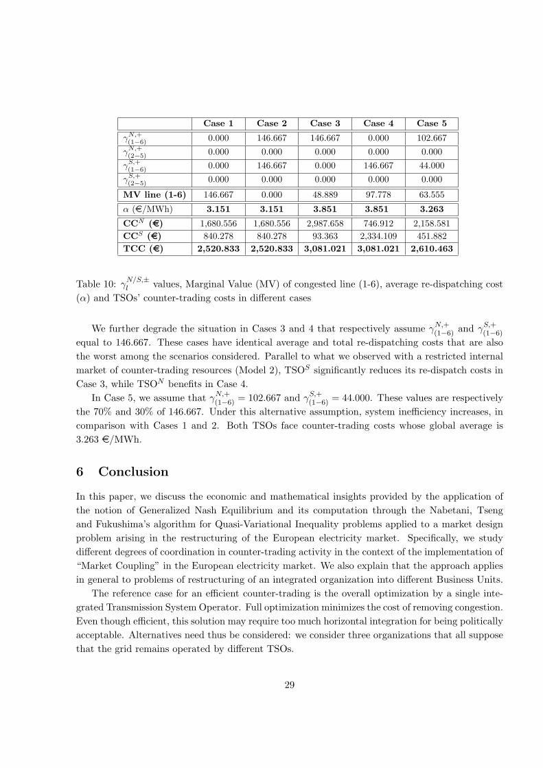
Case 1 Case 2 Case 3 Case 4 Case 5

γN,+(1−6) 0.000 146.667 146.667 0.000 102.667γN,+(2−5) 0.000 0.000 0.000 0.000 0.000γS,+(1−6) 0.000 146.667 0.000 146.667 44.000γS,+(2−5) 0.000 0.000 0.000 0.000 0.000

MV line (1-6) 146.667 0.000 48.889 97.778 63.555

α (e/MWh) 3.151 3.151 3.851 3.851 3.263

CCN (e) 1,680.556 1,680.556 2,987.658 746.912 2,158.581CCS (e) 840.278 840.278 93.363 2,334.109 451.882TCC (e) 2,520.833 2,520.833 3,081.021 3,081.021 2,610.463

Table 10: γN/S,±l values, Marginal Value (MV) of congested line (1-6), average re-dispatching cost(α) and TSOs’ counter-trading costs in different cases

We further degrade the situation in Cases 3 and 4 that respectively assume γN,+(1−6) and γS,+(1−6)

equal to 146.667. These cases have identical average and total re-dispatching costs that are alsothe worst among the scenarios considered. Parallel to what we observed with a restricted internalmarket of counter-trading resources (Model 2), TSOS significantly reduces its re-dispatch costs inCase 3, while TSON benefits in Case 4.

In Case 5, we assume that γN,+(1−6) = 102.667 and γS,+(1−6) = 44.000. These values are respectivelythe 70% and 30% of 146.667. Under this alternative assumption, system inefficiency increases, incomparison with Cases 1 and 2. Both TSOs face counter-trading costs whose global average is3.263 e/MWh.

6 Conclusion

In this paper, we discuss the economic and mathematical insights provided by the application ofthe notion of Generalized Nash Equilibrium and its computation through the Nabetani, Tsengand Fukushima’s algorithm for Quasi-Variational Inequality problems applied to a market designproblem arising in the restructuring of the European electricity market. Specifically, we studydifferent degrees of coordination in counter-trading activity in the context of the implementation of“Market Coupling” in the European electricity market. We also explain that the approach appliesin general to problems of restructuring of an integrated organization into different Business Units.

The reference case for an efficient counter-trading is the overall optimization by a single inte-grated Transmission System Operator. Full optimization minimizes the cost of removing congestion.Even though efficient, this solution may require too much horizontal integration for being politicallyacceptable. Alternatives need thus be considered: we consider three organizations that all supposethat the grid remains operated by different TSOs.

29

The first case is what we call an internal market of counter-trading resources. Following up oncurrent attempts in European circles to get integrated ancillary services like balancing or reserve, wesuppose that an operators can resort to any counter-trading resource in the market whether in theirjurisdictions or outside. We show that we reproduce the result of the full optimization. This findingalso has an interesting mathematical interpretation. It singles out an unusual situation where thesolution set of a variational inequality problem (in our case the perfectly coordinated counter-trading problem) coincides with that of the corresponding quasi-variational inequality problem(when all players have an un-discriminatory access at identical price to all market shared resources).The economic interpretation is also useful: the un-discriminatory access to the same set of counter-trading resources “completes the market” and hence makes it efficient. Last but not least therecourse to the NTF algorithm offers a neat explanation of why this happens: even though theorganization appears to be of the imperfect coordination type, it may in fact be economicallyefficient because of the arbitrage taking place in the procurement of counter-trading resources.

Any restriction to the internal market of counter-trading resources degrades the situation. Afirst degradation happens if operators can only resort in a limited way to counter-trading resourcesoutside of their jurisdiction. The situation can be improved by creating a market of transmissionservices at the counter-trading level, but full efficiency will only be restored in very particular cases.Here again, the resort to the NTF algorithm makes this analysis particularly easy.

The last case is the one where the market of counter-trading resources is fully segmented.Efficiency is further deteriorated even though the introduction of a common market of transmissionresources can again help.

We conduct all the analysis on a simple six nodes region model, but the results are general.Specifically, the recourse to the NTF algorithm only requires solving an optimal power flow problem.This is now a standard model, which shows that the analysis can be conducted for any real worldproblem.

References

[1] Arrow, K.J., G. Debreu. 1954. Existence of an equilibrium for a competitive economy. Econo-metrica, 22, 265-893.

[2] Chao, H.P., S.C. Peck. 1998. Reliability management in competitive electricity markets. Jour-nal of Regulatory Economics, 14, 198-200.

[3] Debreu G. 1952. A social equilibrium existence theorem. Proc. nat. Acad. Sci. 38, 886-290.

[4] Facchinei F., C. Kanzow. 2007. Generalized Nash equilibrium problems. 4OR, 5, 173-210.

[5] Fukushima M. 2008. Restricted generalized Nash equilibria and controlled penaltymethod.Computational Management Sciences, DOI: 10.1007/s10287-009-0097-4.

30

[6] Harker P.T. 1991. Generalized Nash games and quasi-variational inequalities. European Journalof Operation Research, 54, 81-94.

[7] Nabetani K., P. Tseng, M. Fukushima (2009). Parametrized variational inequality approachesto generalized Nash equilibrium problems with shared constraints. Computational Optimizationand Applications, DOI 10.1007/s10589-009-9256-3.

[8] Oggioni G., Y. Smeers. 2010a. Degree of coordination in market coupling and counter-trading.CORE Discussion Paper, 01.

[9] Oggioni G., Y. Smeers. 2010b. Market Coupling and the organization of counter-trading: sep-arating energy and transmission again? Mimeo.

[10] Pang J.S., M. Fukushima. 2005. Quasi-variational inequalities, generalized Nash equilibria,and multi-leader-follower games. Computational Management Sciences, 2, 21–56.

[11] Ralph D.; Y. Smeers. 2006. EPECs as models for electricity markets. Invited Paper, PowerSystems Conference and Exposition (PSCE). DOI: 10.1109/PSCE.2006.296252, 74–80.

[12] Rosen J.B., 1965. Existence and uniqueness of equilibrium points for concave N-person games.Econometrica, 33, 520-534.

[13] Smeers Y., J.Y. Wei. 1999. Spatial oligopolistic electricity models with Cournot generatorsand regulated transmission prices. Operations Research, 47, 102-112.

[14] Williamson, Oliver E. 1981. The Economics of Organization: The Transaction Cost Approach.The American Journal of Sociology, 87(3), 548-577.

Appendix A: Market coupling model

When PXs and TSOs are not integrated, PXs clear the energy markets on the basis of a simplifiedrepresentation of the transmission grid that TSOs give them. This organization of the energy marketis known as market-coupling (MC). Market coupling is the most advanced version of cross-bordertrade implemented in Europe. It is currently applied in France, Belgium and the Netherlands andsoon it will be extended to Germany. According to our problem formulation, PXs operate in acoordinated way, but they clear a market organized as depicted in Figure 2. The objective function(101) includes the average re-dispatching costs α. We here suppose that the TSO costs are paidthrough a levy α charged through the PX. This assumption is introduced for the sake of convenienceand does not restrict in any way the scope of the model. We also assume in this example that itis paid by the generators (the reality is that this levy is largely charged to the consumer side, butthis distinction is immaterial for our purpose) and then this levy is proportional to the quantityinjected in the energy market. Conditions (102) and (103) express the energy balance in Northern

31

and in the Southern zone respectively. The free variable I indicates the import/export betweenthe two zones. The shadow variables φN,S are the marginal energy prices of the Northern andSouthern zones respectively. Constraints (104) and (105) impose that flow I respects the transferlimit I of the interconnecting line in the two possible directions. The dual variables δ1 and δ2 arethe marginal costs of utilization of this zonal link. Finally, the non-negativity of variables qn isrequired.

Minqn

∑i=1,2,4

∫ qi

0ci(ξ)dξ −

∑j=3,5,6

∫ qj

0wj(ξ)dξ + α · (q1 + q2 + q4) (101)

s.t.q1 + q2 − q3 − I = 0 (φN ) (102)

q4 − q5 − q6 + I = 0 (φS) (103)

I − I ≥ 0 (δ1) (104)

I + I ≥ 0 (δ2) (105)

qn ≥ 0 ∀n (106)

Appendix B: Complementarity conditions of the perfectly coordi-

nated counter-trading model

Consider the complementarity formulation of problem (59)-(65), as indicated below, where λl =(−λ+

l + λ−l )

0 ≤ ci(qi + ∆qi)− λl ·∑l

PTDFi,l − µ1 + µ2⊥(qi + ∆qi) ≥ 0 i = 1, 2, 4 (107)

0 ≤ −ωj(q3 + ∆qj) + λl ·∑l

PTDF3,l − µ1 − µ2⊥(qj + ∆qj) ≥ 0 j = 3, 5, 6 (108)

0 ≤ F l − [∑

i=1,2,4

PTDFi,l(qi + ∆qi)−∑

j=3,5,6

PTDFj,l(qj + ∆qj)]⊥λ+l ≥ 0 (109)

0 ≤ F l + [∑

i=1,2,4

PTDFi,l(qi + ∆qi)−∑

j=3,5,6

PTDFj,l(qj + ∆qj)]⊥λ−l ≥ 0 (110)

∑i

∆qi +∑j

∆qj = 0 (µ1) (111)

∑i

∆qi −∑j

∆qj = 0 (µ2) (112)

where ci(qi + ∆qi) =∂

∫ qi+∆qiqi

ci

∂∆qifor i = 1, 2, 4 and −ωj(qj + ∆qj) =

∂∫ qj+∆qjqj

wj

∂∆qjfor j = 3, 5, 6.

32

Appendix C: TSOS’ s problem in the decentralized counter-trading

Model 1

The problem (113)-(118) solved by TSOS is similar to that of the TSON . Its formulation is asfollows:

Min∆qSn

∑i=1,2,4

∫ qi+∆qNi +∆qSi

qi+∆qNi

ci(ξ)dξ −∑

j=3,5,6

∫ qj+∆qNj +∆qSj

qj+∆qNj

wj(ξ)dξ (113)

s.t. ∑i=1,2,4

∆qSi +∑

j=3,5,6

∆qSj = 0 (µS,1) (114)

∑j=3,5,6

∆qSj −∑

i=1,2,4

∆qSi = 0 (µS,2) (115)

F l − [∑

i=1,2,4

PTDFi,l(qi + ∆qNi + ∆qSi )−∑

j=3,5,6

PTDFj,l(qj + ∆qNj + ∆qSj )] ≥ 0 (λS,+l ) (116)

F l + [∑

i=1,2,4

PTDFi,l(qi + ∆qNi + ∆qSi )−∑

j=3,5,6

PTDFj,l(qj + ∆qNj + ∆qSj )] ≥ 0 (λS,−l ) (117)

where l = (1− 6), (2− 5)

qn + ∆qNn + ∆qSn ≥ 0 n = 1, ..., 6 (νSn ) (118)

Appendix D: Complementarity conditions of the imperfectly coor-

dinated counter-trading Model 1

We here present the mixed complementarity formulation of the decentralized counter-trading Model1 (72)-(80). Setting γNl = (−γN,+l + γN,−l ); γSl = (−γS,+l + γS,−l ) and λl = (−λ+

l + λ−l ) forl = ((1− 6), (2− 5)), the complementarity conditions are as follows:

0 ≤ ci(qi + ∆qNi + ∆qSi )−∑l

(λl + γNl ) · PTDFi,l − µN,1 + µN,2⊥(qi + ∆qNi + ∆qSi ) ≥ 0 (119)

0 ≤ −wj(qj + ∆qNj + ∆qSj ) +∑l

(λl + γNl ) · PTDFj,l − µN,1 − µN,2⊥(qj + ∆qNj + ∆qSj ) ≥ 0 (120)

0 ≤ ci(qi + ∆qNi + ∆qSi )−∑l

(λl + γSl ) · PTDFi,l − µS,1 + µS,2⊥(qi + ∆qNi + ∆qSi ) ≥ 0 (121)

33

0 ≤ −wj(qj + ∆qNj + ∆qSj ) +∑l

(λl + γSl ) · PTDFj,l − µS,1 − µS,2⊥(qj + ∆qNj + ∆qSj ) ≥ 0 (122)

0 ≤ F l − [∑

i=1,2,4

PTDFi,l(qi + ∆qNi + ∆qSi )−∑

j=3,5,6

PTDFj,l(qj + ∆qNj + ∆qSj )⊥λ+l ] ≥ 0 (123)

0 ≤ F l + [∑

i=1,2,4

PTDFi,l(qi + ∆qNi + ∆qSi )−∑

j=3,5,6

PTDFj,l(qj + ∆qNj + ∆qSj )⊥λ−l ] ≥ 0 (124)

∑i=1,2,4

∆qNi +∑

j=3,5,6

∆qNj = 0 (µN,1) (125)

∑j=3,5,6

∆qNj −∑

i=1,2,4

∆qNi = 0 (µN,2) (126)

∑i=1,2,4

∆qSi +∑

j=3,5,6

∆qSj = 0 (µS,1) (127)

∑j=3,5,6

∆qSj −∑

i=1,2,4

∆qSi = 0 (µS,2) (128)

where i = 1, 2, 4; j = 3, 5, 6 and the dual variables µN,1, µS,1, µN,2 and µS,2 associated withequality constraints are free variables. Moreover, it holds that (see proof of Proposition 2):

ci(qi + ∆qNi + ∆qSi ) =∂∫ qi+∆qNi +∆qSiqi

ci

∂∆qNi=∂∫ qi+∆qNi +∆qSiqi

ci

∂∆qSii = 1, 2, 4 (129)

wj(qj + ∆qNj + ∆qSj ) =∂∫ qj+∆qNj +∆qSjqj

wj

∂∆qNj=∂∫ qj+∆qNj +∆qSjqj

wj

∂∆qSjj = 3, 5, 6 (130)

Note that conditions (119), (120), (125) and (126) exclusively refer to TSON , while (121),(122), (127) and (128) are those of TSOS . Finally, (123) and (124) are the common transmissionconstraints.

Appendix E: Proof of Proposition 1

Because all constraints are linear, constraint qualification holds. Following Theorem 3.3 of [7],⟨g(x∗), γi

⟩= 0 (131)

is a necessary and sufficient condition for a solution x∗ to problem V I(F γ ,K) to be a GNE.Suppose this property holds for a solution of the parametrized problem (72)-(80). It is then a

GNE and we can write the KKT conditions of that parametrized problem (see the complementarityconditions in Appendix D). Suppose that qn + ∆qNn + ∆qSn > 0 for all n and that λl = (−λ+

l + λ−l )

34

in order to simplify the discussion. Then the optimality condition in (119)-(122) are binding andit follows that:

ci(qi + ∆qNi + ∆qSi )−∑l

γNl PTDFi,l −∑l

λl · PTDFi,l − µN,1 + µN,2 = 0 (132)

−wj(qj + ∆qNj + ∆qSj ) +∑l

γNl PTDFj,l +∑l

λl · PTDFj,l − µN,1 − µN,2 = 0 (133)

ci(qi + ∆qNi + ∆qSi )−∑l

γSl PTDFi,l −∑l

λl · PTDFi,l − µS,1 + µS,2 = 0 (134)

−wj(qj + ∆qNj + ∆qSj ) +∑l

γSl PTDFj,l +∑l

λl · PTDFj,l − µS,1 − µS,2 = 0 (135)

Subtracting (134) from (132) and (135) from (133) leads to the following conditions:∑l

(γNl − γSl )PTDFi,l = −(µN,1 − µN,2) + (µS,1 − µS,2) i = 1, 2, 4 (136)

∑l

(γNl − γSl )PTDFj,l = (µN,1 + µN,2)− (µS,1 + µS,2) j = 3, 5, 6 (137)

Because node 6 is the hub, we have PTDF6,l = 0 and hence (µN,1 + µN,2) − (µS,1 + µS,2) = 0in (137). This in turn implies (γN(1−6) − γ

S(1−6))PTDFj,(1−6) + (γN(2−5) − γ

S(2−5))PTDFj,(2−5) = 0 for

j = 3, 5 and then:

(γN(1−6) − γS(1−6)) = −

PTDFj,(2−5)

PTDFj,(1−6)(γN(2−5) − γ

S(2−5)) j = 3, 5 (138)

This is verified only when γNl = γSl because the ratio PTDFj,(2−5)

PTDFj,(1−6)assumes a positive and a

negative value. Taking stock of condition (131), we can deduce that:

γN,+l = γS,+l

γN,−l = γS,−l

�

Appendix F: Proof of Proposition 2

Assume again in order to simplify the discussion that qn + ∆qNn + ∆qSn > 0 ∀n and define λNl =(−λN,+l +λN,−l ) and λSl = (−λS,+l +λS,−l ) for l = ((1−6), (2−5)). We state the KKT conditions ofthe problems of the two TSOs’ problems (namely (66)-(71) for TSON and (113)-(118) for TSOS)by deriving with respect to the variables ∆qNn and ∆qSn . We get:

35

∂∫ qi+∆qNi +∆qSiqi

ci

∂∆qZi−∑l

λZl PTDFi,l − µZ,1 + µZ,2 = 0 i = 1, 2, 4 Z = N,S (139)

−∂∫ qj+∆qNj +∆qSjqj

wj

∂∆qZj+∑l

λZl PTDFj,l − µZ,1 − µZ,2 = 0 j = 3, 5, 6 Z = N,S (140)

From (139) and (140), we can immediately deduce that:

∂∫ qi+∆qNi +∆qSiqi

ci

∂∆qNi=∂∫ qi+∆qNi +∆qSiqi

ci

∂∆qSi= ci(qi + ∆qNi + ∆qSi ) i = 1, 2, 4 (141)

∂∫ qj+∆qNj +∆qSjqj

wj

∂∆qNj=∂∫ qj+∆qNj +∆qSjqj

wj

∂∆qSj= −wj(qj + ∆qNj + ∆qSj ) j = 3, 5, 6 (142)

and summing (139) to (140), we have:

ci(qi+∆qNi +∆qSi )−wj(qj+∆qNj +∆qSj )+∑l

λZl (PTDFj,l−PTDFi,l)−2µZ,1 = 0 Z = N,S (143)

Since condition (143) holds for both TSOs, we can rewrite it in an explicit way:

ci(qi + ∆qNi + ∆qSi )− wj(qj + ∆qNj + ∆qSj ) +∑l

λNl (PTDFj,l − PTDFi,l)− 2µN,1 = 0 (144)

ci(qi + ∆qNi + ∆qSi )− wj(qj + ∆qNj + ∆qSj ) +∑l

λSl (PTDFj,l − PTDFi,l)− 2µS,1 = 0 (145)

Taking into account the results of conditions (141) and (142) and subtracting (145) from (144),we get: ∑

l

(λNl − λSl )(PTDFj,l − PTDFi,l)− 2(µN,1 − µS,1) = 0 (146)

We now subtract (140) from (139) and apply the above reasoning. We get:

ci(qi+∆qNi +∆qSi )+wj(qj+∆qNj +∆qSj )−∑l

λZl (PTDFj,l+PTDFi,l)+2µZ,2 = 0 Z = N,S (147)

that can be substituted by these two conditions:

ci(qi + ∆qNi + ∆qSi ) + wj(qj + ∆qNj + ∆qSj )−∑l

λNl (PTDFj,l + PTDFi,l) + 2µN,2 = 0 (148)

36

ci(qi + ∆qNi + ∆qSi ) + wj(qj + ∆qNj + ∆qSj )−∑l

λSl (PTDFj,l + PTDFi,l) + 2µS,2 = 0 (149)

Again, taking stock of conditions (141) and (142), (148) and (149) become:∑l

(λNl − λSl )(PTDFj,l + PTDFi,l)− 2(µN,2 − µS,2) = 0 (150)

The combination of conditions (146) and (150) leads to the following equalities:∑l

(λNl − λSl )PTDFj,l − (µN,1 − µS,1)− (µN,2 − µS,2) = 0 (151)

∑l

(λNl − λSl )PTDFi,l + (µN,1 − µS,1)− (µN,2 − µS,2) = 0 (152)

By setting, α = (µN,1 +µN,2)− (µS,1 +µS,2) and β = (µN,1−µN,2)− (µS,1−µS,2) conditions (151)and (152) become: ∑

l

(λNl − λSl )PTDFj,l − α = 0 j = 3, 5, 6 (153)

∑l

(λNl − λSl )PTDFi,l + β = 0 i = 1, 2, 4 (154)

We observe that PTDF6,l = 0. This implies that α = 0. If α = 0, then it holds that:∑l

(λNl − λSl )PTDFj,l = 0 j = 3, 5 (155)

This corresponds to:

(λN(1−6) − λS(1−6))PTDFj,(1−6) + (λN(2−5) − λ

S(2−5))PTDFj,(2−5) = 0 j = 3, 5 (156)

(λN(1−6) − λS(1−6)) = −

PTDFj,(2−5)

PTDFj,(1−6)(λN(2−5) − λ

S(2−5)) j = 3, 5 (157)

But PTDFj,(2−5)

PTDFj,(1−6)assumes a positive and a negative value respectively for j = 3, 5 and then λNl = λSl .

This result means that the marginal value of congestion of one line is identical for both TSOs.Consequently, the two TSOs are implicitly coordinated and there is no arbitrage. This also impliesthat α = β = 0 and then:

(µN,1 + µN,2)− (µS,1 + µS,2) = 0 (158)

(µN,1 − µN,2)− (µS,1 − µS,2) = 0 (159)

These can be rewritten as follows:

µN,1 − µS,1 = (µS,2 − µN,2) (160)

37

µN,1 − µS,1 = −(µS,2 − µN,2) = 0 (161)

This implies that µN,1 = µS,1 and µN,2 = µS,2. �

Appendix G: Proof of Corollary 1

Corollary 3.2 of Nabetani, Tseng and Fukushima’s paper (see [7]) proves that if the dual problemhas solution then ⋃

γ∈Γ

SOLV I(Fγ ,K) ⊇ SOLGNEP

We first consider the case where γ = 0. Under this assumption V I(F,K) = V I(F γ=0,K) and theparametrized problem is identical to the optimized counter-trading problem. This can be easilydone by imposing ∆qNn + ∆qSn = ∆qn.

As already observed, the optimized counter-trading problem has a unique solution because ofthe convexity of the set K and the strict convexity of its objective function. This implies that thesolution of the decentralized counter-trading problem (72)-(80) coincides with that of the optimizedcounter-trading model (59)-(65) when γ = 0.

We now show that the solution set of problem V I(F γ ,K) when γN,±l = γS,±l and µZ,1 = µZ,2

reduces to a unique solution that is the solution of the optimized counter-trading problem (59)-(65).Compare now the KKT conditions of the optimized counter-trading problem with those of the

decentralized counter-trading problem. Denote ∆qn = ∆qNn + ∆qSn for all n and λl = (−λ+l +

λ−l ), the optimality conditions of the optimized counter-trading model are as follows (comparecomplementarity conditions in Appendix B):

ci(qi + ∆qNi + ∆qSi )−∑l

λlPTDFi,l − µ1 + µ2 = 0 i = 1, 2, 4 (162)

−wj(qj + ∆qNj + ∆qSj ) +∑l

λlPTDFj,l − µ1 − µ2 = 0 j = 3, 5, 6 (163)

+ transmission constraints and the re-dispatching balances.

Denoting similarly γNl = (−γN,+l + γN,−l ) γSl = (−γS,+l + γS,−l ) and knowing that γN,±l = γS,±l ,the optimality conditions of the decentralized counter-trading Model 1 are as follows:

ci(qi + ∆qNi + ∆qSi )−∑l

(λl + γNl )PTDFi,l − µ1 + µ2 = 0 i = 1, 2, 4 (164)

−wj(qj + ∆qNj + ∆qSj ) +∑l

(λl + γNl )PTDFj,l − µ1 − µ2 = 0 j = 3, 5, 6 (165)

+ transmission constraints and the re-dispatching balances.

Setting λl = λl + γNl one can easily see that the two groups of optimality conditions are identicaland then the corresponding problems admit the same solution set.

38

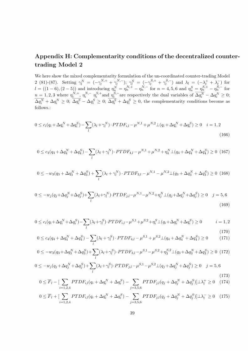
Appendix H: Complementarity conditions of the decentralized counter-

trading Model 2

We here show the mixed complementarity formulation of the un-coordinated counter-trading Model2 (81)-(87). Setting γNl = (−γN,+l + γN,−l ); γSl = (−γS,+l + γS,−l ) and λl = (−λ+

l + λ−l ) forl = ((1 − 6), (2 − 5)) and introducing ηNn = ηN,+n − ηN,−n for n = 4, 5, 6 and ηSn = ηS,+n − ηS,−n forn = 1, 2, 3 where ηN,+i , ηN,−i ηS,+i and ηS,−i are respectively the dual variables of ∆qNi − ∆qNi ≥ 0;∆qNi + ∆qNi ≥ 0; ∆qSi − ∆qSi ≥ 0; ∆qSi + ∆qSi ≥ 0, the complementarity conditions become asfollows.:

0 ≤ ci(qi+∆qNi +∆qSi )−∑l

(λl+γNl ) ·PTDFi,l−µN,1 +µN,2⊥(qi+∆qNi +∆qSi ) ≥ 0 i = 1, 2

(166)

0 ≤ c4(q4 +∆qN4 +∆qS4 )−∑l

(λl+γNl ) ·PTDF4,l−µN,1 +µN,2 +ηN4 ⊥(q4 +∆qN4 +∆qS4 ) ≥ 0 (167)

0 ≤ −w3(q3 + ∆qN3 + ∆qS3 ) +∑l

(λl + γNl ) ·PTDF3,l − µN,1 − µN,2⊥(q3 + ∆qN3 + ∆qS3 ) ≥ 0 (168)

0 ≤ −wj(qj+∆qNj +∆qSj )+∑l

(λl+γNl )·PTDFj,l−µN,1−µN,2+ηNj ⊥(qj+∆qNj +∆qSj ) ≥ 0 j = 5, 6

(169)

0 ≤ ci(qi+∆qNi +∆qSi )−∑l

(λl+γSl )·PTDFi,l−µS,1+µS,2+ηSi ⊥(qi+∆qNi +∆qSi ) ≥ 0 i = 1, 2

(170)0 ≤ c4(q4 + ∆qN4 + ∆qS4 )−

∑l

(λl + γSl ) ·PTDF4,l−µS,1 +µS,2⊥(q4 + ∆qN4 + ∆qS4 ) ≥ 0 (171)

0 ≤ −w3(q3 +∆qN3 +∆qS3 )+∑l

(λl+γSl )·PTDF3,l−µS,1−µS,2 +ηS,23 ⊥(q3 +∆qN3 +∆qS3 ) ≥ 0 (172)

0 ≤ −wj(qj+∆qNj +∆qSj )+∑l

(λl+γSl )·PTDFj,l−µS,1−µS,2⊥(qj+∆qNj +∆qSj ) ≥ 0 j = 5, 6

(173)0 ≤ F l − [

∑i=1,2,4

PTDFi,l(qi + ∆qNi + ∆qSi )−∑

j=3,5,6

PTDFj,l(qj + ∆qNj + ∆qSj )]⊥λ+l ≥ 0 (174)

0 ≤ F l + [∑

i=1,2,4

PTDFi,l(qi + ∆qNi + ∆qSi )−∑

j=3,5,6

PTDFj,l(qj + ∆qNj + ∆qSj )]⊥λ−l ≥ 0 (175)

39

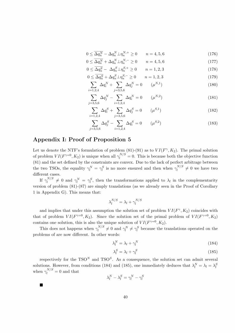
0 ≤ ∆qNn −∆qNn ⊥ηN,+n ≥ 0 n = 4, 5, 6 (176)

0 ≤ ∆qNn + ∆qNn ⊥ηN,−n ≥ 0 n = 4, 5, 6 (177)

0 ≤ ∆qSn − ∆qSn⊥ηS,+n ≥ 0 n = 1, 2, 3 (178)

0 ≤ ∆qSn + ∆qSn⊥ηS,−n ≥ 0 n = 1, 2, 3 (179)∑i=1,2,4

∆qNi +∑

j=3,5,6

∆qNj = 0 (µN,1) (180)

∑j=3,5,6

∆qNj −∑

i=1,2,4

∆qNi = 0 (µN,2) (181)

∑i=1,2,4

∆qSi +∑

j=3,5,6

∆qSj = 0 (µS,1) (182)

∑j=3,5,6

∆qSj −∑

i=1,2,4

∆qSi = 0 (µS,2) (183)

Appendix I: Proof of Proposition 5

Let us denote the NTF’s formulation of problem (81)-(91) as to V I(F γ ,K2). The primal solutionof problem V I(F γ=0,K2) is unique when all γN/Sl = 0. This is because both the objective function(81) and the set defined by the constraints are convex. Due to the lack of perfect arbitrage betweenthe two TSOs, the equality γNl = γSl is no more ensured and then when γ

N/Sl 6= 0 we have two

different cases.If γN/Sl 6= 0 and γNl = γSl , then the transformations applied to λl in the complementarity

version of problem (81)-(87) are simply translations (as we already seen in the Proof of Corollary1 in Appendix G). This means that:

λN/Sl = λl + γ

N/Sl

and implies that under this assumption the solution set of problem V I(F γ ,K2) coincides withthat of problem V I(F γ=0,K2). Since the solution set of the primal problem of V I(F γ=0,K2)contains one solution, this is also the unique solution of V I(F γ=0,K2).

This does not happens when γN/Sl 6= 0 and γNl 6= γSl because the translations operated on the

problems of are now different. In other words:

λNl = λl + γNl (184)

λSl = λl + γSl (185)

respectively for the TSON and TSOS . As a consequence, the solution set can admit severalsolutions. However, from conditions (184) and (185), one immediately deduces that λNl = λl = λSlwhen γ

N/Sl = 0 and that

λNl − λSl = γNl − γSl�

40

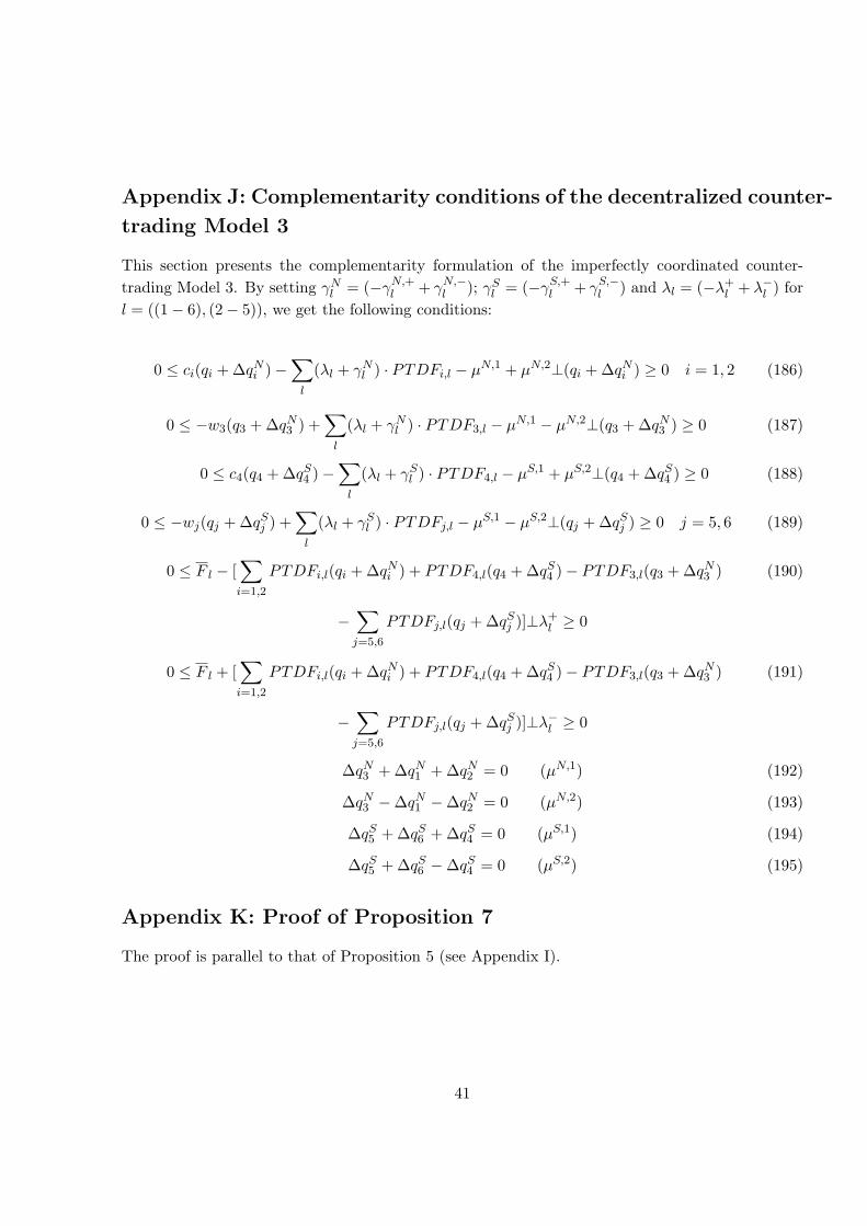
Appendix J: Complementarity conditions of the decentralized counter-

trading Model 3

This section presents the complementarity formulation of the imperfectly coordinated counter-trading Model 3. By setting γNl = (−γN,+l + γN,−l ); γSl = (−γS,+l + γS,−l ) and λl = (−λ+

l + λ−l ) forl = ((1− 6), (2− 5)), we get the following conditions:

0 ≤ ci(qi + ∆qNi )−∑l

(λl + γNl ) · PTDFi,l − µN,1 + µN,2⊥(qi + ∆qNi ) ≥ 0 i = 1, 2 (186)

0 ≤ −w3(q3 + ∆qN3 ) +∑l

(λl + γNl ) · PTDF3,l − µN,1 − µN,2⊥(q3 + ∆qN3 ) ≥ 0 (187)

0 ≤ c4(q4 + ∆qS4 )−∑l

(λl + γSl ) · PTDF4,l − µS,1 + µS,2⊥(q4 + ∆qS4 ) ≥ 0 (188)

0 ≤ −wj(qj + ∆qSj ) +∑l

(λl + γSl ) · PTDFj,l − µS,1 − µS,2⊥(qj + ∆qSj ) ≥ 0 j = 5, 6 (189)

0 ≤ F l − [∑i=1,2

PTDFi,l(qi + ∆qNi ) + PTDF4,l(q4 + ∆qS4 )− PTDF3,l(q3 + ∆qN3 ) (190)

−∑j=5,6

PTDFj,l(qj + ∆qSj )]⊥λ+l ≥ 0

0 ≤ F l + [∑i=1,2

PTDFi,l(qi + ∆qNi ) + PTDF4,l(q4 + ∆qS4 )− PTDF3,l(q3 + ∆qN3 ) (191)

−∑j=5,6

PTDFj,l(qj + ∆qSj )]⊥λ−l ≥ 0

∆qN3 + ∆qN1 + ∆qN2 = 0 (µN,1) (192)

∆qN3 −∆qN1 −∆qN2 = 0 (µN,2) (193)

∆qS5 + ∆qS6 + ∆qS4 = 0 (µS,1) (194)

∆qS5 + ∆qS6 −∆qS4 = 0 (µS,2) (195)

Appendix K: Proof of Proposition 7

The proof is parallel to that of Proposition 5 (see Appendix I).

41