Generalized Multi-view Shared Subspace Learning using View

Generalized Multi-view Shared Subspace Learning using View Bootstrapping

Krishna Somandepalli 1 Shrikanth Narayanan 1

Abstract

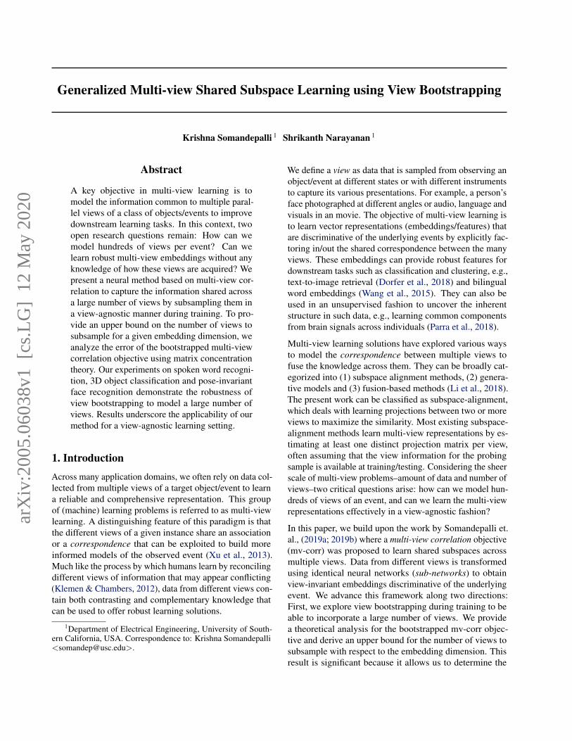
A key objective in multi-view learning is tomodel the information common to multiple paral-lel views of a class of objects/events to improvedownstream learning tasks. In this context, twoopen research questions remain: How can wemodel hundreds of views per event? Can welearn robust multi-view embeddings without anyknowledge of how these views are acquired? Wepresent a neural method based on multi-view cor-relation to capture the information shared acrossa large number of views by subsampling them ina view-agnostic manner during training. To pro-vide an upper bound on the number of views tosubsample for a given embedding dimension, weanalyze the error of the bootstrapped multi-viewcorrelation objective using matrix concentrationtheory. Our experiments on spoken word recogni-tion, 3D object classification and pose-invariantface recognition demonstrate the robustness ofview bootstrapping to model a large number ofviews. Results underscore the applicability of ourmethod for a view-agnostic learning setting.

1. IntroductionAcross many application domains, we often rely on data col-lected from multiple views of a target object/event to learna reliable and comprehensive representation. This groupof (machine) learning problems is referred to as multi-viewlearning. A distinguishing feature of this paradigm is thatthe different views of a given instance share an associationor a correspondence that can be exploited to build moreinformed models of the observed event (Xu et al., 2013).Much like the process by which humans learn by reconcilingdifferent views of information that may appear conflicting(Klemen & Chambers, 2012), data from different views con-tain both contrasting and complementary knowledge thatcan be used to offer robust learning solutions.

1Department of Electrical Engineering, University of South-ern California, USA. Correspondence to: Krishna Somandepalli<[email protected]>.

We define a view as data that is sampled from observing anobject/event at different states or with different instrumentsto capture its various presentations. For example, a person’sface photographed at different angles or audio, language andvisuals in an movie. The objective of multi-view learning isto learn vector representations (embeddings/features) thatare discriminative of the underlying events by explicitly fac-toring in/out the shared correspondence between the manyviews. These embeddings can provide robust features fordownstream tasks such as classification and clustering, e.g.,text-to-image retrieval (Dorfer et al., 2018) and bilingualword embeddings (Wang et al., 2015). They can also beused in an unsupervised fashion to uncover the inherentstructure in such data, e.g., learning common componentsfrom brain signals across individuals (Parra et al., 2018).

Multi-view learning solutions have explored various waysto model the correspondence between multiple views tofuse the knowledge across them. They can be broadly cat-egorized into (1) subspace alignment methods, (2) genera-tive models and (3) fusion-based methods (Li et al., 2018).The present work can be classified as subspace-alignment,which deals with learning projections between two or moreviews to maximize the similarity. Most existing subspace-alignment methods learn multi-view representations by es-timating at least one distinct projection matrix per view,often assuming that the view information for the probingsample is available at training/testing. Considering the sheerscale of multi-view problems–amount of data and number ofviews–two critical questions arise: how can we model hun-dreds of views of an event, and can we learn the multi-viewrepresentations effectively in a view-agnostic fashion?

In this paper, we build upon the work by Somandepalli et.al., (2019a; 2019b) where a multi-view correlation objective(mv-corr) was proposed to learn shared subspaces acrossmultiple views. Data from different views is transformedusing identical neural networks (sub-networks) to obtainview-invariant embeddings discriminative of the underlyingevent. We advance this framework along two directions:First, we explore view bootstrapping during training to beable to incorporate a large number of views. We providea theoretical analysis for the bootstrapped mv-corr objec-tive and derive an upper bound for the number of views tosubsample with respect to the embedding dimension. Thisresult is significant because it allows us to determine the

arX

iv:2

005.

0603

8v1

[cs

.LG

] 1

2 M

ay 2

020


number of sub-networks to use in the mv-corr framework.

Second, we conduct several experiments to benchmark theperformance of view-bootstrapping for downstream learningtasks and highlight its applicability for modeling a largenumber of views in a view-agnostic fashion. In practice,this framework only needs to know that the sample of viewsconsidered at each training iteration have a correspondence.That is, the multiple views are obtained from observing thesame underlying event. A natural example for this settingis audio recordings from multiple microphones distributedin a conference room. In this example, we can use thetimestamps to construct a correspondence. This method canalso be used for applications such as pose-invariant facerecognition in a semi-supervised setting. We do not needthe pose information (view-agnostic) or the total numberof classes during training. All we need to know is that thedifferent face images are of the same person.

2. Related Work2.1. Subspace alignment for more than two views

Widely used correlation-based methods include canonicalcorrelation analysis (CCA) (Hotelling, 1992) and its deeplearning versions (Andrew et al., 2013; Dumpala et al., 2018)that can learn non-linear transformations of the two viewsto derive maximally correlated subspaces. Several metric-learning based methods were proposed to extend CCA formultiple views by learning a view-specific or view-invariantfeature space by transforming data. For example, general-ized CCA (Horst, 1961; Benton et al., 2017) and multi-viewCCA (Chaudhuri et al., 2009). Their applications includeaudio-visual speaker clustering and phoneme classificationfrom speech and articulatory information.

In a supervised setting, a discriminative multi-view sub-space can be obtained by treating labels as an additionalview. Prominent examples of this idea include generalizedmulti-view analysis (GMA, Sharma et al. 2012), partialleast squares regression based methods (Cai et al., 2013)and multi-view discriminant analysis (MvDA, Kan et al.(2015)). They were effectively used for applications such asimage captioning and pose-invariant face recognition. How-ever the generalizability of these methods to hundreds ofviews remains to be explored.

2.2. View-agnostic multi-view learning

The subspace methods discussed thus far assume that theview information is readily available during training andtesting. For instance, GMA and MvDA estimate a within-class scatter matrix specific to each view. In practice, viewinformation may not be available for the probe data (e.g.,pose of a face during testing). A promising direction toaddress this problem was proposed by Ding and Fu (2014;

2017). To eliminate the need for view information of theprobe sample, a low-rank subspace representation was usedto bridge the view-specific and view-invariant representa-tions. Here, a single projection matrix per view was usedwhich would scale linearly with increasing number of views.

2.3. Domain adaptation in a multi-view paradigm

A recent survey by Ding et al. (2018) presents a unifiedlearning framework mapping out the similarities betweenmulti-view learning and domain adaptation. Typical domainadaptation methods seek domain-invariant representationswhich are akin to view-invariant representations if we treatdifferent domains as views. The benefit of the multi-viewparadigm in this context is that the variabilities associatedwith multiple views can be washed out to obtain discrimina-tive representations of the underlying classes.

This formulation is particularly useful in the domain ofspeech/audio processing for applications such as wake-wordrecognition (Kepuska & Klein, 2009). Here we need to rec-ognize a keyword (e.g., “Alexa”, “OK Google”, “Siri”) nomatter who says it or where it is said (i.e., the specific back-ground acoustic conditions). Speaker verification methodsbased on joint factor analysis (Dehak et al., 2009) and totalvariability modeling (Dehak et al., 2011) have explored theideas of factoring out the speaker-dependent factors andspeaker-independent factors to obtain robust speaker repre-sentations in the context of domain adaption. Recently, So-mandepalli et al. (2019a) showed that a more robust speechrepresentation can be obtained by explicitly modeling mul-tiple utterances of a word as corresponding views.

2.4. Views vs. Modalities

Following ideas proposed in the review by Ding et al. (2018),we delineate two kinds of allied but distinct learning prob-lems: multi-view and multi-modal. In related work of thisdomain (See surveys by Zhao et al. 2017; Ding et al. 2018;Li et al. 2018), the two terms are used interchangeably. Wehowever distinguish the two concepts to facilitate modelingand analysis. Multiple views of an event can be modeledas samples drawn from identically distributed random pro-cesses, e.g., a person’s face at different poses. However,the individual modalities in multi-modal data need not arisefrom identically distributed processes, e.g., person’s identityfrom their voice, speech and pose.

In this work, we focus on multi-view problems, specificallyto learn embeddings that capture the shared informationacross the views. The premise that multiple views canbe modeled as samples from identically distributed pro-cesses not only facilitates the theoretical analysis of themv-corr objective, but also helps us to formulate domainadaptation problems in a multi-view paradigm; particularly,for applications that need to scale for hundreds of views


(e.g., speaker-invariant word recognition). While it shouldbe noted that the methods explored in this work may notbe directly applied to multi-modal problems where we aregenerally interested to capture both modality-specific andmodality-shared representations, the theory developed inthis work can be extended to other methods such as GMA(Sharma et al., 2012) and multi-view deep network (Kanet al., 2016) for the broader class of multi-modal problems.

3. Proposed ApproachWe first review the multi-view correlation (mv-corr) objec-tive developed by Somandepalli et. al., (2019a; 2019b).Next, we consider practical aspects for using this ob-jective in a deep learning framework followed by view-bootstrapping. Then, we develop a theoretical analysis tounderstand the error of the bootstrapped mv-corr objective.

3.1. Multi-view correlation (mv-corr)

Consider N samples of d-dimensional features sampledby observing an object/event from M different views. LetXl ∈ Rd×N : l = 1, ...,M , be the data matrix for the l-thview with columns as mean-zero features. We can use thesame feature dimension d across all views because we as-sume that that the multiple views are sampled from identicaldistributions (See Sec. 2.4). We describe the mv-corr objec-tive in the context of CCA. The premise of applying CCA-like approaches to multi-view learning is that the inherentvariability associated with a semantic class is uncorrelatedacross multiple views to represent the signal shared acrossthe views. For M = 2, CCA finds projections of samedimensions v1 and v2 in the direction that maximizes thecorrelation between them. Formally,

(v∗1,v∗2) = argmax

v1,v2∈Rd

v>1 Σ12v2√v>1 Σ11v1v>2 Σ22v2

(1)

where Σ12 is the cross-covariance and Σ11 ,Σ22 are thecovariance terms for the two views. To extend the CCAformulation for more than two views, we consider the sumof all pairwise covariance terms. That is, find a projectionmatrix or a multi-view shared subspace W ∈ Rk×d thatmaximizes the ratio of the sum of between-view over within-view covariances in the projected space:

W∗ = argmaxW

W>(X1X>2 + . . .+ XM−1X

>M

)W

W>(X1X>1 + . . .+ XMX>M

)W

(2)

We refer to the numerator and denominator covariance sumsin Eq. 2 as between-view covariance Rb and within-viewcovariance Rw which are sums of M(M − 1) and M co-variance terms, respectively. Because we assume featurecolumns in Xl to be mean-zero, we estimate the covariancematrices as a cross product without loss of generality.

We now define a multi-view correlation Λ as the normalizedratio of between- and within-view covariance matrix:

Λ = maxW

1

M − 1

W>RbW

W>RwW(3)

here, the common scaling factorM(N−1) in the covarianceestimates are omitted from the ratio.

A version of this ratio of covariances has been consideredin several related multi-view learning methods. One ofthe earliest works by Hotelling (1992) presented a similarformulation for scalars, also referred to as multi-set CCA bysome works (e.g., Parra et al. 2018). Notice that this ratio issimilar to the use of between-class and within-class scattermatrices in linear discriminant analysis (LDA, Fisher 1936)and more recently in multi-view methods such as GMA andMvDA. Another version of this ratio known as the intraclasscorrelation coefficient (Bartko, 1966) has been extensivelyused to quantify test-retest repeatability of clinical measures(e.g., Somandepalli et al. 2015).

The primary difference of mv-corr formulation from thesemethods is that it does not consider the class informationexplicitly while estimating the covariance matrices. All weneed to know is that the subset of M views correspond tothe same object/event. Additionally we consider the sumof covariances for all pairs of views, eliminating the needfor view-specific transformation which enables us to learnthe shared subspace W in a view-agnostic manner. On thedownside, we only capture the shared representation acrossmultiple views and discard view-specific information whichmay be of interest for some multi-modal applications.

3.2. Implementation and practical considerations

Using ideas similar to the deep variants of CCA (Andrewet al., 2013) and LDA (Dorfer et al., 2015), we can use deepneural networks (DNN) to learn non-linear transformationsof the multi-view data to obtain (possibly) low-dimensionalrepresentations. In Eq. 9, the solution W jointly diagonal-izes the two covariances Rb and Rw because W is theircommon eigenspace. Thus, we use the trace (Tr) form ofEq. 9 to fashion a loss function, ρM for batch optimizationin DNN for data from M views.

ρM = maxW

1

d(M − 1)

Tr(W>RbW

)Tr(W>RwW)

(4)

The DNN framework for mv-corr consists of one networkper view l, referred to as lth sub-network denoted by fl.The architecture of the sub-network is the same for mul-tiple views and the weights are not shared across the sub-networks for any layer. The output from the top-most layerof each sub-network is passed to a fully-connected layer ofd neurons. Let Hl = fl(Xl) ∈ Rd×N be the activations


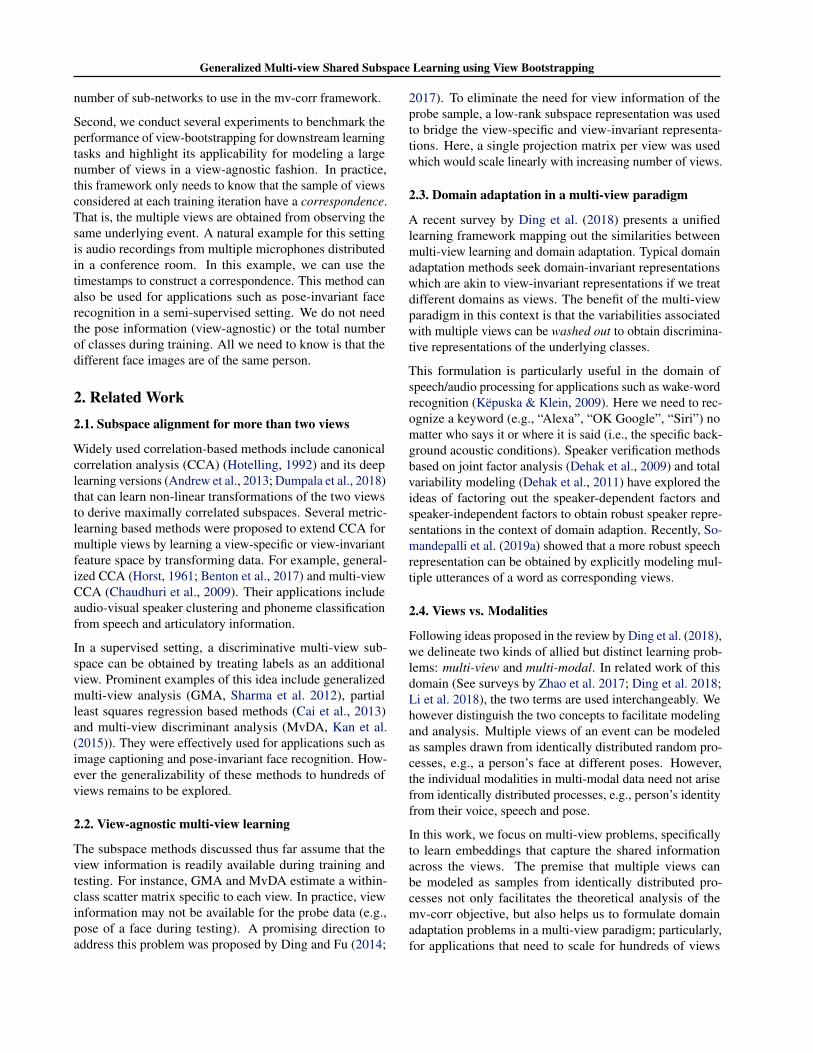
Figure 1. Schematic of view bootstrapping for multi-view shared subspace learning. Inset: example sub-network architecture

from this last layer where N is now the batch size. Thus, foreach batch we estimate the between- and within-view co-variances Rb and Rw using Hl , l = 1, . . . ,M to computethe loss in Eq. 8. The subspace W is obtained by solvingthe generalized eigenvalue (GEV) problem using Choleskydecomposition.

Total view covariance: For a large number of views M ,estimating Rb in each batch is expensive as it is O(M2).We instead compute a total-view covariance term Rt whichonly involves estimating a single covariance for the sum ofall views and is O(M), and then estimate Rb = Rt −Rw.See Supplementary (Suppl.) methods S1 for the proof.

Rt = Rb + Rw =1

M

( M∑l=1

Xl

)( M∑l=1

Xl

)>(5)

Choosing batch size: A sample size of O(d log d) is suffi-cient to approximate the sample covariance matrix of a gen-eral distribution in Rd (Vershynin, 2010). Thus we choosea batch size of N = ceil(d log d) for a network with d-dimensional embeddings. In our experiments, choosingN < d log d was detrimental to model convergence.

Regularize Rw: Maximizing ρM (Eq. 8) corresponds tomaximizing the mean of eigenvalues of R−1w Rb. EstimatingRw with rank deficient Hl may lead to spuriously high ρ.One solution is to truncate the eigenspace W. However,this will reduce the number of directions of separability inthe data. To retain the full dimensionality of the covariancematrix, we use “shrinkage” regularization (Ledoit & Wolf,2004) for Rw with a parameter ν = 0.2 and normalizedtrace parameter λ = Tr(Rw) as Rw = (1−ν)Rw+νλId/d

Loss function is bounded: The objective ρM is the averageof d eigenvalues obtained by solving GEV. We can analyti-cally show that this objective is bounded above by 1 (SeeSuppl. methods S2). Thus, during training, we minimizethe loss 1− ρM to avoid trivial solutions.

Inference: Maximizing ρ leads to maximally correlatedembeddings. Thus, during inference we only need to extractembeddings from one of the sub-networks. The proposed

loss ensures that the different embeddings are maximallycorrelated (See Suppl. methods simulations S3).

3.3. View bootstrapping

Modeling a large number of views would require many sub-networks which is not practical for hundreds of views. Toaddress this issue, we propose view bootstrapping. Theschematic of the overall method is shown in Figure 1. Here,we construct a network with m sub-networks and samplewith replacement a small number of views m � M tomodel data with M views. During training, we do notkeep track of views being sampled for specific sub-networkswhich ensures that the model is view-agnostic. The boot-strapped objective can be written as:

ρ∗ = Em∼U(1,M)ρm ≈ ρM (6)

The intuition behind our stochastic extension lies in law oflarge numbers applied to the covariance matrices in Eq. 8.Let R{b,w} now denote the covariances estimated from mviews. Asymptotically, with a large M and as m→M , wehave ER

(m)b → Σb and ER

(m)w → Σw where Σb and Σw

are the between- and within-view covariance estimated forall M views. In practice, the number of available view sam-ples is finite and the total number of views possible is oftenunknown. Thus, we analyze the error of the estimate ρmwith respect to ρ∗ = d−1 Tr

(W>ΣbW

)/Tr

(W>ΣwW

)in a non-asymptotic setting.

Theorem 3.1. Let X = [A(1), . . . ,A(N)] be the m × dmatrices of m views sampled from an unknown numberof views M . Let the rows Al of the view matrices A beindependent subgaussian vectors in Rd with ‖Al‖2 = 1 :l = 1, . . . ,m. Then for any t ≥ 0, with probability at least1− 2 exp

(−ct2

), we have

ρm ≤ max

(1, C

m2

(√d+ t)2

ρ∗)

Here, ρm and ρ∗ are the mv-corr objectives for subsampledviews m and the total number of views M respectively. The


constant C depends only on the subgaussian norm K of theview space, with K = max

i,l

∥∥∥A(i)l

∥∥∥ψ2

Proof sketch. Here we highlight the main elements of theproof. Please see Suppl. methods, Theorem S6 for the de-tailed work. Recall that Rb and Rw now denote covariancematrices for m views. Using properties of trace and spectralnorm, we can rewrite the expression of the correspondingρm as:

ρm =Tr(W>RbW

)Tr(W>RwW)

=〈Rb + Σb −Σb,WW>〉〈Rw + Σw −Σw,WW>〉

≤ 〈Σb,WW>〉+ ‖Rt −Σt‖+ ‖Rw −Σw‖〈Σw,WW>〉 − ‖Rw −Σw‖

where Σb and Σw are the previously defined between- andwithin-view covariances respectively for M views. FromEq. 5, recall the result: Rb = Rt − Rw. The rest fol-lows through triangular inequalities. Observe that the ra-tio 〈ΣB ,WW>〉/〈ΣW ,WW>〉 is the optimal ρ∗ esti-mated from the unknown number of views M . Also, thetwo trace terms are sum of normalized eigenvalues. Thus∣∣〈Σb,WW>〉

∣∣, ∣∣〈ΣW ,WW>〉∣∣ ∈ [1, d].

Next, we need to bound the two norms δt = ‖Rt −Σt‖and δw = ‖Rw −Σw‖. In the statement of the theorem,note that the multi-view data matrix X was rearranged as[A(1), . . . ,A(N)] using the features as rows in the view-matrices A. Thus, using the identicality assumption ofmultiple views, we have:

δw =

∥∥∥∥∥N∑i=1

1

mA(i)>A(i) − EA(i)>A(i)

∥∥∥∥∥≤

N∑i=1

∥∥∥∥ 1

mA(i)>A(i) −Σ(i)

w

∥∥∥∥ ≤ N∥∥∥∥ 1

mA>A−Σw

∥∥∥∥The term

∥∥ 1mA>A−Σw

∥∥ has been extensively studied forthe case of isotropic distributions i.e., Σw = I by Vershynin(2010). Here, we obtain a bound for the general case of Σw

and show that δw = ‖Rw −Σw‖ is O(d/m). Similarly,we can show that δt = ‖Rt −Σt‖ ≤ m. The intuition hereis that Rt is sum of m view vectors, hence it is O(m). De-tailed proofs for δw and δt are provided in Suppl. methods,Lemmas S4 and S5. Using these results and the fact that wealways choose an embedding dimension d greater than m,we can prove that ρm is O(m2/d).

This result is significant because we can now show that, toobtain d-dimensional multi-view embeddings, we only needto subsample m ≤

√d number of views from the larger set

of views. For example, for a 64-dimensional embedding, wewould need to sample at most 8 views. In other words, theDNN architecture in this case would have 8 sub-networks.

2 3 4 5 7 9

50

60

70

80

m <√d, d = 40

View bootstrap sample size m

Clu

ster

ing

acc.

(%)f

orun

seen

view

s

d = 16d = 32d = 40d = 64

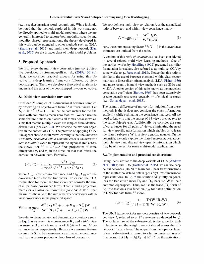
Figure 2. Clustering accuracy of unseen views for different choicesof embedding-dimension d and number of views subsampled m

Additionally, the choice of d is important because a smalld would only discriminate between classes that are alreadyeasily separable in the data. In contrast, a larger d wouldrequire a greater m which in turn inflates the number ofparameters in the DNN.

4. ExperimentsWe conducted experiments with three different datasets tobenchmark the performance of our method with respectto the competitive baselines specific to these domains. Wechose these datasets to assess the applicability of our methodfor downstream learning tasks in two distinct multi-classsemi-supervised settings: (1) uniform distribution of viewsper class and (2) variable number of views per class.

4.1. 3D object classification

We use Princeton ModelNet dataset (Wu et al., 2015) toclassify the object type from 2D images acquired at multipleview points. We use the train/test splits for the 40-classsubset provided in their website1. Each class has 100 CADmodels (80/20 for train/test) with 2D images (100× 100px)rendered in two settings by Su et al. (2015): V-12: 12 viewsby placing virtual cameras at 30 degree intervals around theconsistent upright position of an object and V-80: 80 viewsrendered by placing 20 cameras pointed towards the objectcentroid and rotating at 0, 90, 180, 270 degrees along theaxis passing through the camera and the object centroid.

4.1.1. DEEP MV-CORR MODEL

As shown in Figure 1, we use identical sub-networks tomodel the data from each view. The number of sub-networksis equal to the number of views subsampled m. We use asimple 3-block VGG architecture (Chatfield et al., 2014) asillustrated in the inset in Figure 1. To reduce the number of

13D object dataset and leader-board:modelnet.cs.princeton.edu


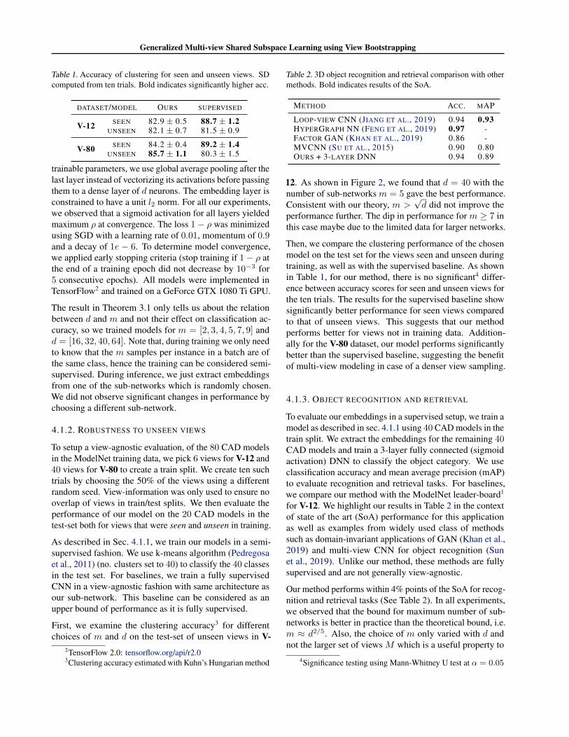
Table 1. Accuracy of clustering for seen and unseen views. SDcomputed from ten trials. Bold indicates significantly higher acc.

DATASET/MODEL OURS SUPERVISED

V-12 SEEN 82.9 ± 0.5 88.7 ± 1.2UNSEEN 82.1 ± 0.7 81.5 ± 0.9

V-80 SEEN 84.2 ± 0.4 89.2 ± 1.4UNSEEN 85.7 ± 1.1 80.3 ± 1.5

trainable parameters, we use global average pooling after thelast layer instead of vectorizing its activations before passingthem to a dense layer of d neurons. The embedding layer isconstrained to have a unit l2 norm. For all our experiments,we observed that a sigmoid activation for all layers yieldedmaximum ρ at convergence. The loss 1− ρ was minimizedusing SGD with a learning rate of 0.01, momentum of 0.9and a decay of 1e − 6. To determine model convergence,we applied early stopping criteria (stop training if 1− ρ atthe end of a training epoch did not decrease by 10−3 for5 consecutive epochs). All models were implemented inTensorFlow2 and trained on a GeForce GTX 1080 Ti GPU.

The result in Theorem 3.1 only tells us about the relationbetween d and m and not their effect on classification ac-curacy, so we trained models for m = [2, 3, 4, 5, 7, 9] andd = [16, 32, 40, 64]. Note that, during training we only needto know that the m samples per instance in a batch are ofthe same class, hence the training can be considered semi-supervised. During inference, we just extract embeddingsfrom one of the sub-networks which is randomly chosen.We did not observe significant changes in performance bychoosing a different sub-network.

4.1.2. ROBUSTNESS TO UNSEEN VIEWS

To setup a view-agnostic evaluation, of the 80 CAD modelsin the ModelNet training data, we pick 6 views for V-12 and40 views for V-80 to create a train split. We create ten suchtrials by choosing the 50% of the views using a differentrandom seed. View-information was only used to ensure nooverlap of views in train/test splits. We then evaluate theperformance of our model on the 20 CAD models in thetest-set both for views that were seen and unseen in training.

As described in Sec. 4.1.1, we train our models in a semi-supervised fashion. We use k-means algorithm (Pedregosaet al., 2011) (no. clusters set to 40) to classify the 40 classesin the test set. For baselines, we train a fully supervisedCNN in a view-agnostic fashion with same architecture asour sub-network. This baseline can be considered as anupper bound of performance as it is fully supervised.

First, we examine the clustering accuracy3 for differentchoices of m and d on the test-set of unseen views in V-

2TensorFlow 2.0: tensorflow.org/api/r2.03Clustering accuracy estimated with Kuhn’s Hungarian method

Table 2. 3D object recognition and retrieval comparison with othermethods. Bold indicates results of the SoA.

METHOD ACC. MAP

LOOP-VIEW CNN (JIANG ET AL., 2019) 0.94 0.93HYPERGRAPH NN (FENG ET AL., 2019) 0.97 -FACTOR GAN (KHAN ET AL., 2019) 0.86 -MVCNN (SU ET AL., 2015) 0.90 0.80OURS + 3-LAYER DNN 0.94 0.89

12. As shown in Figure 2, we found that d = 40 with thenumber of sub-networks m = 5 gave the best performance.Consistent with our theory, m >

√d did not improve the

performance further. The dip in performance for m ≥ 7 inthis case maybe due to the limited data for larger networks.

Then, we compare the clustering performance of the chosenmodel on the test set for the views seen and unseen duringtraining, as well as with the supervised baseline. As shownin Table 1, for our method, there is no significant4 differ-ence between accuracy scores for seen and unseen views forthe ten trials. The results for the supervised baseline showsignificantly better performance for seen views comparedto that of unseen views. This suggests that our methodperforms better for views not in training data. Addition-ally for the V-80 dataset, our model performs significantlybetter than the supervised baseline, suggesting the benefitof multi-view modeling in case of a denser view sampling.

4.1.3. OBJECT RECOGNITION AND RETRIEVAL

To evaluate our embeddings in a supervised setup, we train amodel as described in sec. 4.1.1 using 40 CAD models in thetrain split. We extract the embeddings for the remaining 40CAD models and train a 3-layer fully connected (sigmoidactivation) DNN to classify the object category. We useclassification accuracy and mean average precision (mAP)to evaluate recognition and retrieval tasks. For baselines,we compare our method with the ModelNet leader-board1

for V-12. We highlight our results in Table 2 in the contextof state of the art (SoA) performance for this applicationas well as examples from widely used class of methodssuch as domain-invariant applications of GAN (Khan et al.,2019) and multi-view CNN for object recognition (Sunet al., 2019). Unlike our method, these methods are fullysupervised and are not generally view-agnostic.

Our method performs within 4% points of the SoA for recog-nition and retrieval tasks (See Table 2). In all experiments,we observed that the bound for maximum number of sub-networks is better in practice than the theoretical bound, i.e.m ≈ d2/5. Also, the choice of m only varied with d andnot the larger set of views M which is a useful property to

4Significance testing using Mann-Whitney U test at α = 0.05


note for practical settings. The parameter d however needsto be tuned for classification tasks as it depends on intra-and inter-class variabilities which determine the complexityof the downstream task.

4.2. Pose-invariant face recognition

Robust face recognition is yet another application wheremulti-view learning solutions are attractive because we areinterested in the shared representation across different pre-sentations of a person’s face. For this task, we use theMulti-PIE face database (Gross et al., 2010) which includesface images of 337 subjects in 15 different poses, 20 lightingconditions and 6 expressions across 4 sessions.

In Sec. 4.1, we evaluated our model to classify object cat-egories available for training, but with a focus on the per-formance of seen vs. unseen views during training. In thisexperiment, we wish to test the usefulness of our embed-dings to recognize faces not seen in training. We use asimilar train/test split as in GMA (Sharma et al., 2012) of129 subjects in 5 lighting conditions (1, 4, 7, 12, 17) com-mon to all four sessions as test data and remaining 120subjects in session 01 for training. For performance eval-uation, we use 1-NN matching with normalized euclideandistance similarity score as the metric. The gallery consistedof faces images of the 129 individuals in frontal pose andfrontal lighting and the remaining images from all poses andlighting conditions were used as probes. All images werecropped to contain only the face and resized to 100× 100pixels. No face alignment was performed.

4.2.1. MODEL AND BASELINES

For our model architecture, we first choose m = 2 sub-networks and examine the mv-corr value at convergence fordifferent embedding dimension d. Based on this we pickd = 64. Following our observations in the object classifica-tion task, we choose m = 4 sub-networks. The sub-networkarchitecture is the same as before (See inset Figure 1). Wedid not explore other architectures because our goal herewas to evaluate the use of mv-corr loss and not necessar-ily the best performing model for a specific task. Duringtraining, we sample with replacement, m face images perindividual agnostic to the pose or lighting condition. Formatching experiments, we extract embeddings from a singlerandomly chosen sub-network.

For baselines, we train deep CCA (DCCA Andrew et al.2013) using its implementation5 with the same sub-networkarchitecture as ours. We trained separate DCCA models forfive poses: 15, 30, 45, 60 and 75 degrees. While trainingthe two sub-networks in DCCA, we sample face images ofsubjects across all lighting conditions with a frontal pose for

5Deep-CCA code: github.com/VahidooX/DeepCCA

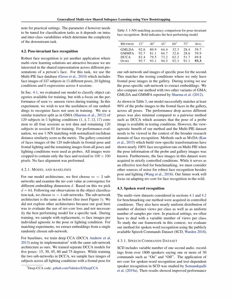
Table 3. 1-NN matching accuracy comparison for pose-invariantface recognition. Bold indicates the best performing model

METHOD 15◦ 30◦ 45◦ 60◦ 75◦ AVG.

GMLDA 92.6 80.9 64.4 32.3 28.4 59.7GMMFA 92.7 81.1 64.7 32.6 28.6 59.9DCCA 82.4 79.5 73.2 62.3 51.7 69.8OURS 95.7 93.1 94.5 92.3 91.1 93.3

one sub-network and images of specific pose for the second.This matches the testing conditions where we only havefrontal pose images in the gallery. During testing we usethe pose-specific sub-network to extract embeddings. Wealso compare our method with two other variants of GMA:GMLDA and GMMFA reported by Sharma et al. (2012).

As shown in Table 3, our model successfully matches at least90% of the probe images to the frontal faces in the gallery,across all poses. The performance drop across differentposes was also minimal compared to a pairwise methodsuch as DCCA which assumes that the pose of a probeimage is available in testing conditions. However, the view-agnostic benefit of our method and the Multi-PIE datasetneeds to be viewed in the context of the broader researchdomain of face recognition. Methods such as MvDA (Kanet al., 2015) which build view-specific transformations haveshown nearly 100% face recognition rate on Multi-PIE whenthe pose information of the probe and gallery images wasknown. Furthermore, the face images in this dataset wereacquired in strictly controlled conditions. While it serves asan effective test-bed for benchmarking, we must considerother sources of noise for robust face recognition besidespose and lighting (Wang et al., 2018). Our future work willfocus on adapting mv-corr for face recognition in-the-wild.

4.3. Spoken word recognition

The multi-view datasets considered in sections 4.1 and 4.2for benchmarking our method were acquired in controlledconditions. They also have nearly uniform distribution ofnumber of distinct views per class as well as as uniformnumber of samples per view. In practical settings, we oftenhave to deal with a variable number of views per class.To study the our framework in this context, we evaluateour method for spoken word recognition using the publiclyavailable Speech Commands Dataset (SCD, Warden 2018).

4.3.1. SPEECH COMMANDS DATASET

SCD includes variable number of one second audio. record-ings from over 1800 speakers saying one or more of 30commands such as “On” and “Off”. The application ofmv-corr for spoken-word recognition and text-dependentspeaker recognition in SCD was studied by Somandepalliet al. (2019a). Their results showed improved performance


dog go tr

ee left on off

upth

ree

cat

bed

seve

nei

ght

four

five

righ

ttw

odo

wn

stop six

nine ye

sho

use no

bird

one

mar

vin

shei

laze

row

owha

ppy

0.4

0.5

0.6

0.7

0.8

Average class acc. = 0.66

Clu

ster

ing

accu

racy

(acc

.)pe

rspe

ech

com

man

d

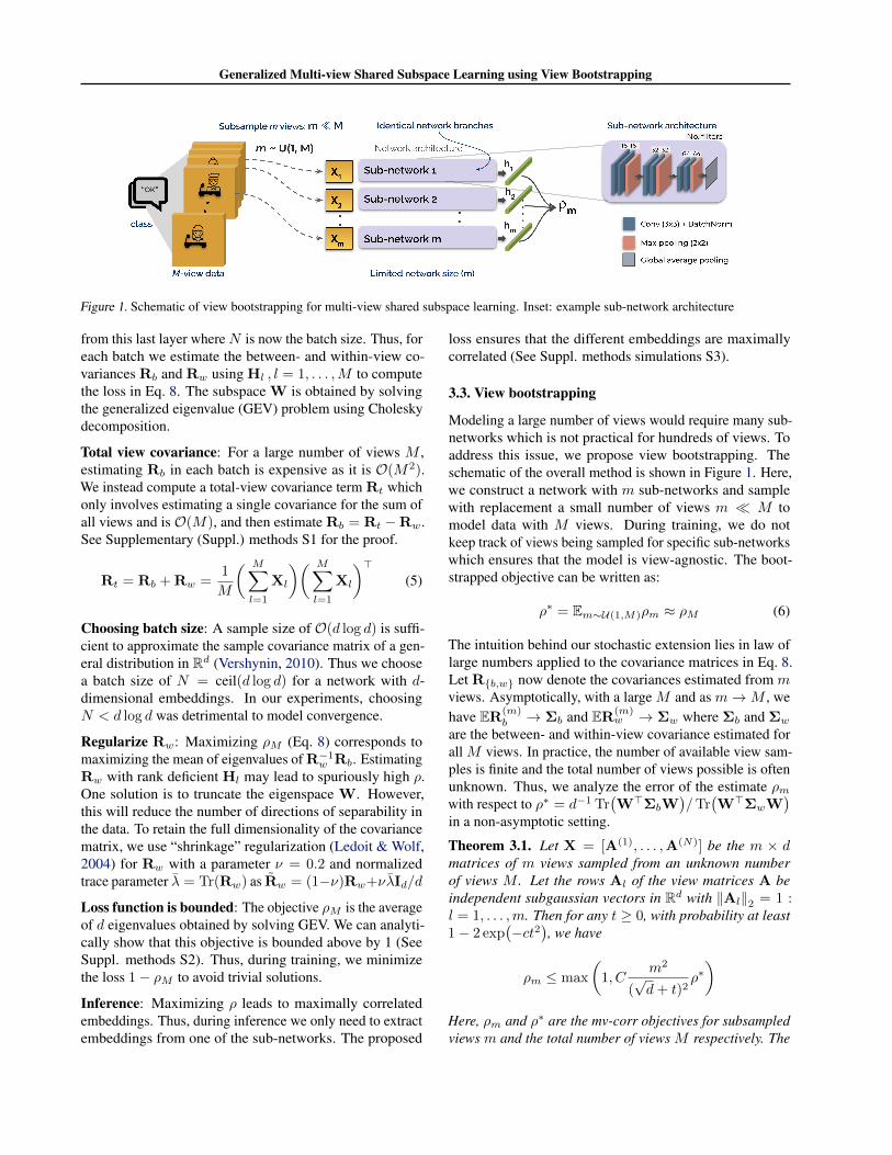
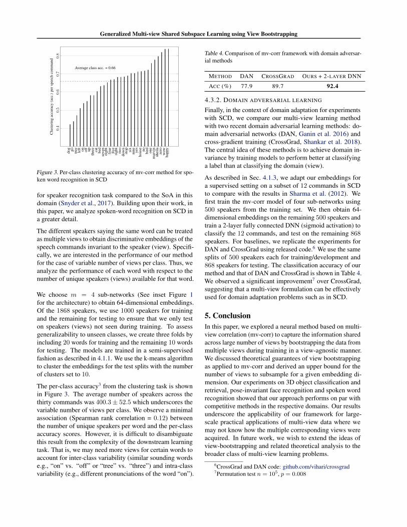
Figure 3. Per-class clustering accuracy of mv-corr method for spo-ken word recognition in SCD

for speaker recognition task compared to the SoA in thisdomain (Snyder et al., 2017). Building upon their work, inthis paper, we analyze spoken-word recognition on SCD ina greater detail.

The different speakers saying the same word can be treatedas multiple views to obtain discriminative embeddings of thespeech commands invariant to the speaker (view). Specifi-cally, we are interested in the performance of our methodfor the case of variable number of views per class. Thus, weanalyze the performance of each word with respect to thenumber of unique speakers (views) available for that word.

We choose m = 4 sub-networks (See inset Figure 1for the architecture) to obtain 64-dimensional embeddings.Of the 1868 speakers, we use 1000 speakers for trainingand the remaining for testing to ensure that we only teston speakers (views) not seen during training. To assessgeneralizability to unseen classes, we create three folds byincluding 20 words for training and the remaining 10 wordsfor testing. The models are trained in a semi-supervisedfashion as described in 4.1.1. We use the k-means algorithmto cluster the embeddings for the test splits with the numberof clusters set to 10.

The per-class accuracy3 from the clustering task is shownin Figure 3. The average number of speakers across thethirty commands was 400.3± 52.5 which underscores thevariable number of views per class. We observe a minimalassociation (Spearman rank correlation = 0.12) betweenthe number of unique speakers per word and the per-classaccuracy scores. However, it is difficult to disambiguatethis result from the complexity of the downstream learningtask. That is, we may need more views for certain words toaccount for inter-class variability (similar sounding wordse.g., “on” vs. “off” or “tree” vs. “three”) and intra-classvariability (e.g., different pronunciations of the word “on”).

Table 4. Comparison of mv-corr framework with domain adversar-ial methods

METHOD DAN CROSSGRAD OURS + 2-LAYER DNN

ACC (%) 77.9 89.7 92.4

4.3.2. DOMAIN ADVERSARIAL LEARNING

Finally, in the context of domain adaptation for experimentswith SCD, we compare our multi-view learning methodwith two recent domain adversarial learning methods: do-main adversarial networks (DAN, Ganin et al. 2016) andcross-gradient training (CrossGrad, Shankar et al. 2018).The central idea of these methods is to achieve domain in-variance by training models to perform better at classifyinga label than at classifying the domain (view).

As described in Sec. 4.1.3, we adapt our embeddings fora supervised setting on a subset of 12 commands in SCDto compare with the results in Sharma et al. (2012). Wefirst train the mv-corr model of four sub-networks using500 speakers from the training set. We then obtain 64-dimensional embeddings on the remaining 500 speakers andtrain a 2-layer fully connected DNN (sigmoid activation) toclassify the 12 commands, and test on the remaining 868speakers. For baselines, we replicate the experiments forDAN and CrossGrad using released code.6 We use the samesplits of 500 speakers each for training/development and868 speakers for testing. The classification accuracy of ourmethod and that of DAN and CrossGrad is shown in Table 4.We observed a significant improvement7 over CrossGrad,suggesting that a multi-view formulation can be effectivelyused for domain adaptation problems such as in SCD.

5. ConclusionIn this paper, we explored a neural method based on multi-view correlation (mv-corr) to capture the information sharedacross large number of views by bootstrapping the data frommultiple views during training in a view-agnostic manner.We discussed theoretical guarantees of view bootstrappingas applied to mv-corr and derived an upper bound for thenumber of views to subsample for a given embedding di-mension. Our experiments on 3D object classification andretrieval, pose-invariant face recognition and spoken wordrecognition showed that our approach performs on par withcompetitive methods in the respective domains. Our resultsunderscore the applicability of our framework for large-scale practical applications of multi-view data where wemay not know how the multiple corresponding views wereacquired. In future work, we wish to extend the ideas ofview-bootstrapping and related theoretical analysis to thebroader class of multi-view learning problems.

6CrossGrad and DAN code: github.com/vihari/crossgrad7Permutation test n = 105, p = 0.008


Supplementary MethodsThe following sections provide detailed proofs for propositions, lemmas and the theorem presented in the associated ICMLsubmission. We also provide details of simulation analysis that we conducted to support one of the claims made in the paper.

Contents

Section Link

Table of Notations 5

Proposition: Total-view Covariance S6

Proposition: Multi-view correlation objective is bounded above by 1 S7

Simulation Experiments S8

Lemma: Upper Bound for Bootstrapped Within-View Covariance S9

Lemma: Upper Bound for Bootstrapped Total-View Covariance S10

Theorem: Error of the Bootstrapped Multi-view Correlation S11


Notation

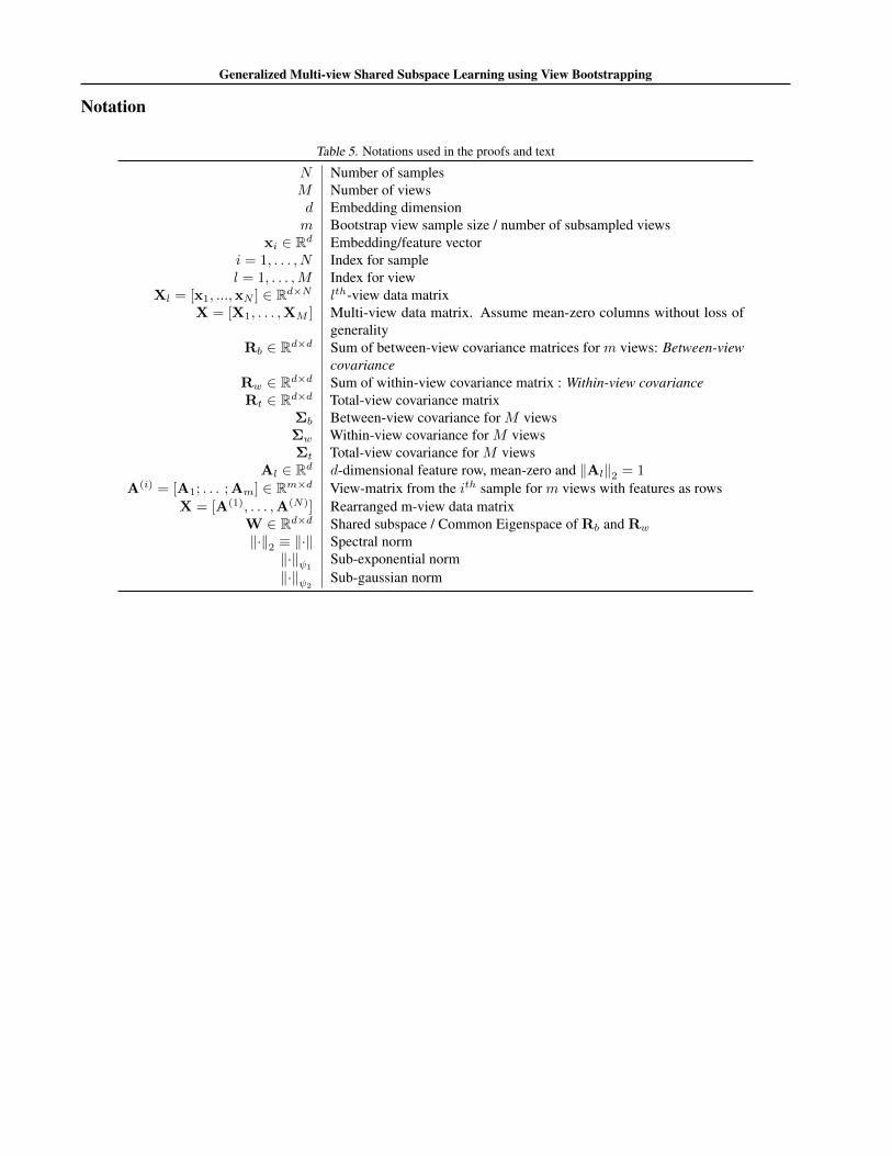
Table 5. Notations used in the proofs and text

N Number of samplesM Number of viewsd Embedding dimensionm Bootstrap view sample size / number of subsampled views

xi ∈ Rd Embedding/feature vectori = 1, . . . , N Index for samplel = 1, . . . ,M Index for view

Xl = [x1, ...,xN ] ∈ Rd×N lth-view data matrixX = [X1, . . . ,XM ] Multi-view data matrix. Assume mean-zero columns without loss of

generalityRb ∈ Rd×d Sum of between-view covariance matrices for m views: Between-view

covarianceRw ∈ Rd×d Sum of within-view covariance matrix : Within-view covarianceRt ∈ Rd×d Total-view covariance matrix

Σb Between-view covariance for M viewsΣw Within-view covariance for M viewsΣt Total-view covariance for M views

Al ∈ Rd d-dimensional feature row, mean-zero and ‖Al‖2 = 1A(i) = [A1; . . . ; Am] ∈ Rm×d View-matrix from the ith sample for m views with features as rows

X = [A(1), . . . ,A(N)] Rearranged m-view data matrixW ∈ Rd×d Shared subspace / Common Eigenspace of Rb and Rw

‖·‖2 ≡ ‖·‖ Spectral norm‖·‖ψ1

Sub-exponential norm‖·‖ψ2

Sub-gaussian norm


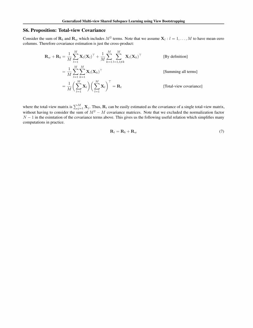
S6. Proposition: Total-view CovarianceConsider the sum of Rb and Rw which includes M2 terms. Note that we assume Xl : l = 1, . . . ,M to have mean-zerocolumns. Therefore covariance estimation is just the cross-product:

Rw + Rb =1

M

M∑l=1

Xl(Xl)> +

1

M

M∑k=1

M∑l=1,l 6=k

Xl(Xk)> [By definition]

=1

M

M∑l=1

M∑k=1

Xl(Xk)> [Summing all terms]

=1

M

( M∑l=1

Xl

)( M∑l=1

Xl

)>= Rt [Total-view covariance]

where the total-view matrix is∑Mj=1 Xj . Thus, Rt can be easily estimated as the covariance of a single total-view matrix,

without having to consider the sum of M2 −M covariance matrices. Note that we excluded the normalization factorN − 1 in the esimtation of the covariance terms above. This gives us the following useful relation which simplifies manycomputations in practice.

Rt = Rb + Rw (7)


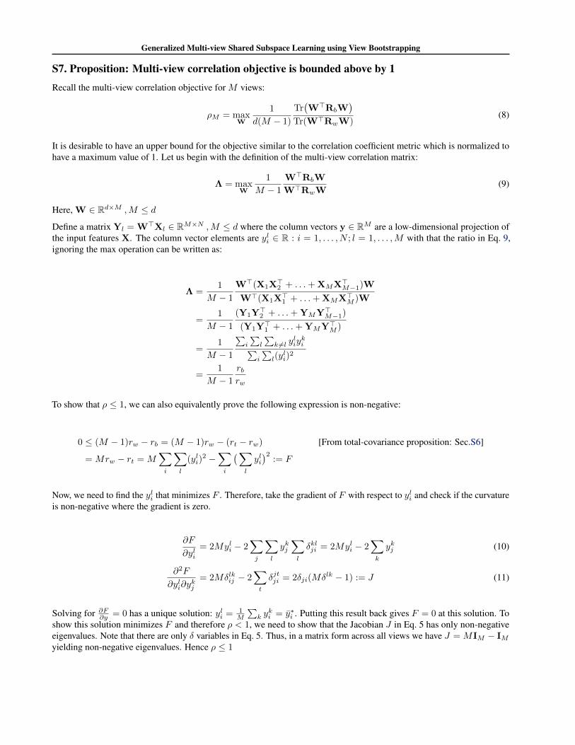
S7. Proposition: Multi-view correlation objective is bounded above by 1Recall the multi-view correlation objective for M views:

ρM = maxW

1

d(M − 1)

Tr(W>RbW

)Tr(W>RwW)

(8)

It is desirable to have an upper bound for the objective similar to the correlation coefficient metric which is normalized tohave a maximum value of 1. Let us begin with the definition of the multi-view correlation matrix:

Λ = maxW

1

M − 1

W>RbW

W>RwW(9)

Here, W ∈ Rd×M ,M ≤ d

Define a matrix Yl = W>Xl ∈ RM×N ,M ≤ d where the column vectors y ∈ RM are a low-dimensional projection ofthe input features X. The column vector elements are yli ∈ R : i = 1, . . . , N ; l = 1, . . . ,M with that the ratio in Eq. 9,ignoring the max operation can be written as:

Λ =1

M − 1

W>(X1X>2 + . . .+ XMX>M−1)W

W>(X1X>1 + . . .+ XMX>M )W

=1

M − 1

(Y1Y>2 + . . .+ YMY>M−1)

(Y1Y>1 + . . .+ YMY>M )

=1

M − 1

∑i

∑l

∑k 6=l y

liyki∑

i

∑l(y

li)

2

=1

M − 1

rbrw

To show that ρ ≤ 1, we can also equivalently prove the following expression is non-negative:

0 ≤ (M − 1)rw − rb = (M − 1)rw − (rt − rw) [From total-covariance proposition: Sec.S6]

= Mrw − rt = M∑i

∑l

(yli)2 −

∑i

(∑l

yli)2

:= F

Now, we need to find the yli that minimizes F . Therefore, take the gradient of F with respect to yli and check if the curvatureis non-negative where the gradient is zero.

∂F

∂yli= 2Myli − 2

∑j

∑l

ykj∑l

δklji = 2Myli − 2∑k

ykj (10)

∂2F

∂yli∂ykj

= 2Mδlkij − 2∑t

δjtji = 2δji(Mδlk − 1) := J (11)

Solving for ∂F∂y = 0 has a unique solution: yli = 1M

∑k y

ki = y∗i . Putting this result back gives F = 0 at this solution. To

show this solution minimizes F and therefore ρ < 1, we need to show that the Jacobian J in Eq. 5 has only non-negativeeigenvalues. Note that there are only δ variables in Eq. 5. Thus, in a matrix form across all views we have J = MIM − IMyielding non-negative eigenvalues. Hence ρ ≤ 1


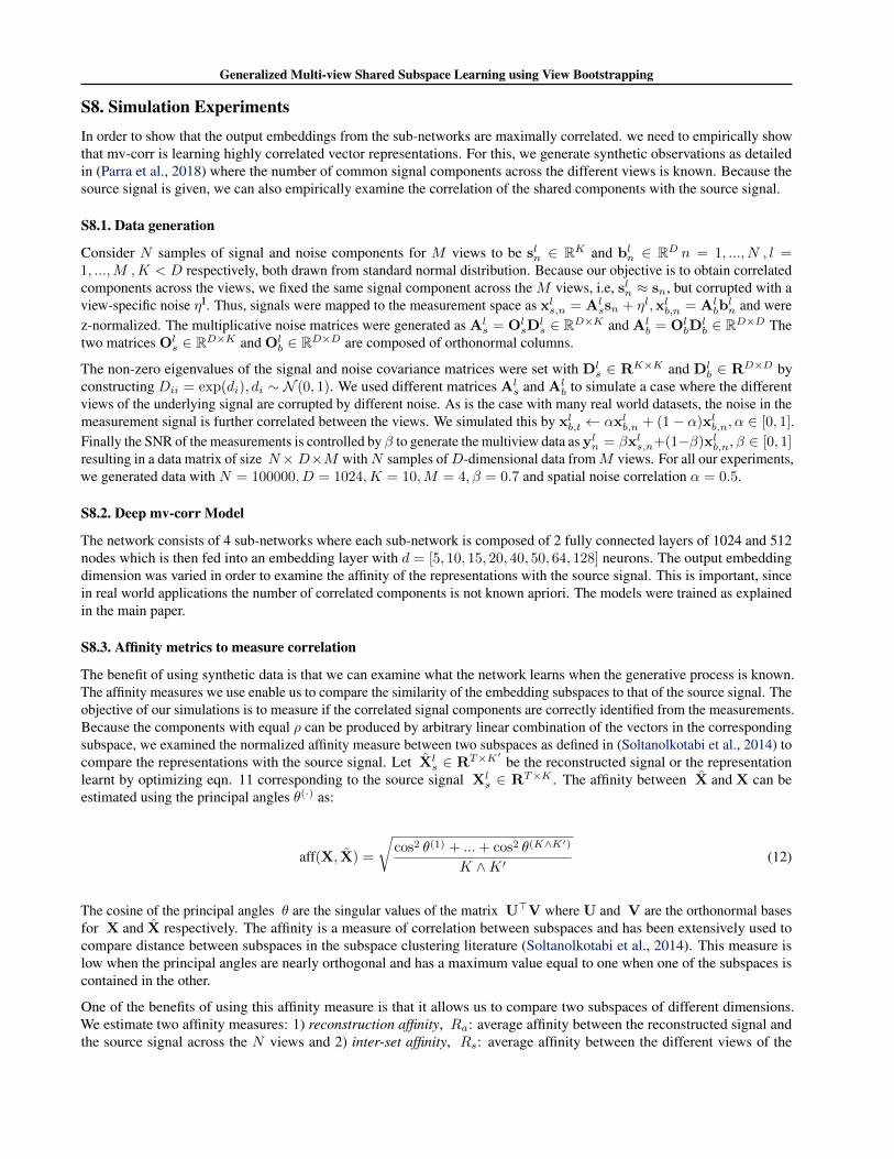
S8. Simulation ExperimentsIn order to show that the output embeddings from the sub-networks are maximally correlated. we need to empirically showthat mv-corr is learning highly correlated vector representations. For this, we generate synthetic observations as detailedin (Parra et al., 2018) where the number of common signal components across the different views is known. Because thesource signal is given, we can also empirically examine the correlation of the shared components with the source signal.

S8.1. Data generation

Consider N samples of signal and noise components for M views to be sln ∈ RK and bln ∈ RD n = 1, ..., N , l =1, ...,M ,K < D respectively, both drawn from standard normal distribution. Because our objective is to obtain correlatedcomponents across the views, we fixed the same signal component across the M views, i.e, sln ≈ sn, but corrupted with aview-specific noise ηl. Thus, signals were mapped to the measurement space as xls,n = Al

ssn + ηl,xlb,n = Albbln and were

z-normalized. The multiplicative noise matrices were generated as Als = Ol

sDls ∈ RD×K and Al

b = OlbD

lb ∈ RD×D The

two matrices Ols ∈ RD×K and Ol

b ∈ RD×D are composed of orthonormal columns.

The non-zero eigenvalues of the signal and noise covariance matrices were set with Dls ∈ RK×K and Dl

b ∈ RD×D byconstructing Dii = exp(di), di ∼ N (0, 1). We used different matrices Al

s and Alb to simulate a case where the different

views of the underlying signal are corrupted by different noise. As is the case with many real world datasets, the noise in themeasurement signal is further correlated between the views. We simulated this by xlb,t ← αxlb,n + (1− α)xlb,n, α ∈ [0, 1].Finally the SNR of the measurements is controlled by β to generate the multiview data as yln = βxls,n+(1−β)xlb,n, β ∈ [0, 1]resulting in a data matrix of size N× D×M withN samples ofD-dimensional data fromM views. For all our experiments,we generated data with N = 100000, D = 1024,K = 10,M = 4, β = 0.7 and spatial noise correlation α = 0.5.

S8.2. Deep mv-corr Model

The network consists of 4 sub-networks where each sub-network is composed of 2 fully connected layers of 1024 and 512nodes which is then fed into an embedding layer with d = [5, 10, 15, 20, 40, 50, 64, 128] neurons. The output embeddingdimension was varied in order to examine the affinity of the representations with the source signal. This is important, sincein real world applications the number of correlated components is not known apriori. The models were trained as explainedin the main paper.

S8.3. Affinity metrics to measure correlation

The benefit of using synthetic data is that we can examine what the network learns when the generative process is known.The affinity measures we use enable us to compare the similarity of the embedding subspaces to that of the source signal. Theobjective of our simulations is to measure if the correlated signal components are correctly identified from the measurements.Because the components with equal ρ can be produced by arbitrary linear combination of the vectors in the correspondingsubspace, we examined the normalized affinity measure between two subspaces as defined in (Soltanolkotabi et al., 2014) tocompare the representations with the source signal. Let Xl

s ∈ RT×K′be the reconstructed signal or the representation

learnt by optimizing eqn. 11 corresponding to the source signal Xls ∈ RT×K . The affinity between X and X can be

estimated using the principal angles θ(·) as:

aff(X, X) =

√cos2 θ(1) + ...+ cos2 θ(K∧K′)

K ∧K ′(12)

The cosine of the principal angles θ are the singular values of the matrix U>V where U and V are the orthonormal basesfor X and X respectively. The affinity is a measure of correlation between subspaces and has been extensively used tocompare distance between subspaces in the subspace clustering literature (Soltanolkotabi et al., 2014). This measure islow when the principal angles are nearly orthogonal and has a maximum value equal to one when one of the subspaces iscontained in the other.

One of the benefits of using this affinity measure is that it allows us to compare two subspaces of different dimensions.We estimate two affinity measures: 1) reconstruction affinity, Ra: average affinity between the reconstructed signal andthe source signal across the N views and 2) inter-set affinity, Rs: average affinity between the different views of the


No.

of d

imen

sion

s, K

Mini-batch size, M

Reconstruction affinity, Ra Inter-set affinity, Rs

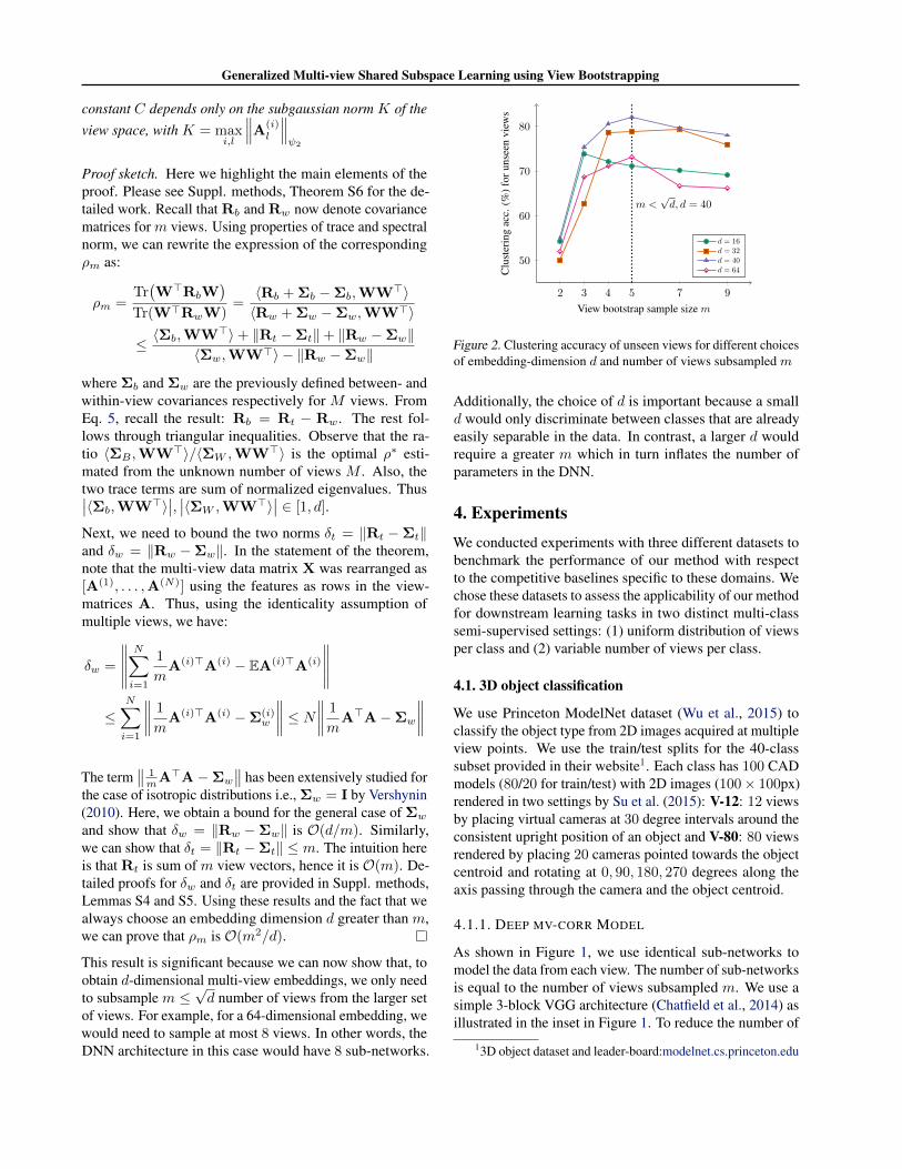
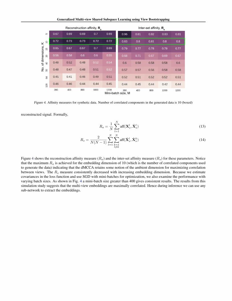
Figure 4. Affinity measures for synthetic data. Number of correlated components in the generated data is 10 (boxed)

reconstructed signal. Formally,

Ra =1

N

N∑l=1

aff(Xls, X

ls) (13)

Rs =2

N(N − 1)

N∑l=1

N∑k=1l 6=k

aff(Xls, X

ks) (14)

Figure 4 shows the reconstruction affinity measure (Ra) and the inter-set affinity measure (Rs) for these parameters. Noticethat the maximum Ra is achieved for the embedding dimension of 10 (which is the number of correlated components usedto generate the data) indicating that the dMCCA retains some notion of the ambient dimension for maximizing correlationbetween views. The Rs measure consistently decreased with increasing embedding dimension. Because we estimatecovariances in the loss function and use SGD with mini-batches for optimization, we also examine the performance withvarying batch sizes. As shown in Fig. 4 a mini-batch size greater than 400 gives consistent results. The results from thissimulation study suggests that the multi-view embeddings are maximally correlated. Hence during inference we can use anysub-network to extract the embeddings.


S9. Lemma: Upper Bound for Bootstrapped Within-View CovarianceLemma S9.1. (Subsampled view matrices, approximate isotropy) Let A be a m×d matrix created by subsampling m viewsfrom a larger, unknown number of views. The rows Ai of the matrix A are independent subgaussian random vectors in Rdand a second moment matrix Σ = EAi ⊗Ai. Then for every t ≥ 0, with probability at least 1− 2 exp

(−ct2

)we have∥∥∥∥ 1

mA>A−Σ

∥∥∥∥ ≤ max(δ, δ2) where δ = C

√d

m+

t√m

(15)

Here C, c > 0 depend only on the subgaussian norm K = maxi ‖Ai‖ψ2of the view space

Proof. This is a straight-forward generalization of Theorem 5.39 (Vershynin, 2010) for non-isotropic spaces. The proofinvolves covering argument which uses a net N to discretize the compact view space, which is all the vectors z in a unitsphere Sd−1. Similar to (Vershynin, 2010), we prove this in three steps:

1. Nε Approximation: Bound the norm ‖Az‖2 for all z ∈ Rd s.t. ‖z‖2 = 1 by discretizing the sphere with a 1/4-net.

2. Concentration: Fix a vector z, and derive a tight bound of ‖Az‖2.

3. Union bound: Take a union bound for all the z in the net

Step 1: Nε Approximation. From (Vershynin, 2010), we use the following statement:

∃δ > 0,∥∥B>B− I

∥∥ ≤ max(δ, δ2) =⇒ ‖B‖2 ≤ 1 + δ (16)

We evaluate the operator norm in eq. 15 as follows:∥∥∥∥ 1

mA>A−Σ

∥∥∥∥ =

∥∥∥∥ 1

mA>A− 1

mEA>A

∥∥∥∥=

∥∥∥∥ 1

mΣmi=1AiA

>i −

1

mΣmi=1EAiA

>i

∥∥∥∥Let D := 1

m

∑mi=1 AiA

>i − 1

mΣmi=1EAiA>i . Choose a ε′-net N such that |N | ≤ 9d which provides sufficient coverage

for the unit sphere Sd−1 at ε′ = 1/4. Then, for every z ∈ N we have (using Lemma 5.4 in (Vershynin, 2010)),

‖D‖ ≤ maxz∈N‖z‖=1

|〈Dz, z〉|

≤ 1

1− 2ε′maxx∈N‖z‖=1

∥∥z>Dz∥∥

≤ 2 maxz∈N

∥∥z>Dz∥∥

For some ε > 0, we want to show that the operator norm of D is concentrated as

maxz∈N

∥∥z>Dz∥∥ ≤ ε

2where ε := max(δ, δ2) (17)

Step 2: Concentration. Fix any vector z ∈ Sd−1 and define Yi = A>i z − EA>i z where Ai are subgaussian randomvectors by assumption with ‖Ai‖ψ2

= K. Thus, Yi i = 1, . . . ,m are independent subgaussian random variables. Thesubgaussian norm of Yi is calculated as,

‖Yi‖ψ2=∥∥A>i z− EA>i z

∥∥ψ2≤ 2∥∥A>i z

∥∥ψ2≤ 2‖Ai‖ψ2

‖z‖ = 2K (18)

The above relation is an application of triangular and Jensen’s inequalities: ‖X − EX‖ ≤ 2‖X‖with |EX| ≤ E|X| ≤ |X| .Similarly, Y 2

i are independent subexponential random variables with the subexponential norm Ke = ‖Yi‖ψ1≤ ‖Yi‖2ψ2

≤4K2. Finally, by definition of Yi, we have ∥∥z>Dz

∥∥ =1

m|Σmi=1Y

2i | (19)


We use the exponential deviation inequality in Corollary 5.17 from (Vershynin, 2010) to control the summation term ineq. 19 to give:

P(∥∥z>Dz

∥∥ ≥ ε

2

)= P

( 1

m|Σmi=1Y

2i | ≥

ε

2

)(20)

≤ 2 exp

[− cmin

(ε2

4K2e

,ε

2Ke

)m

]

Note that ε := max(δ, δ2). If δ ≥ 1 then ε = δ2. Thus, min(ε, ε2) = δ2. Using this and the fact that K ≥ 2‖Yi‖ψ2≥ 1,

we get

P(∥∥z>Dz

∥∥ ≥ ε

2) ≤ 2 exp

[− c1K4

δ2m

]≤ 2 exp

[− c1K4

(C2d+ t2)

](21)

by substituting δ = C√

dm + t√

mand using (a+ b)2 ≥ a2 + b2.

Step 3: Union Bound. Using Boole’s inequality to compute the union bound over all the vectors z in the net N withcardinality |N | = 9d, we get

P

{maxz∈N

∥∥∥∥ 1

mA>A−Σ

∥∥∥∥ ≥ ε

2

}≤ 9d · 2 exp

[− c1K4

(C2d+ t2)

](22)

Pick a sufficiently large C = CK ≥ K2√

log 9/c1, then the probability

P

{maxz∈N

∥∥∥∥ 1

mA>A−Σ

∥∥∥∥ ≥ ε

2

}≤ 2

exp(d+ c1t2

K4

) (23)

≤ 2 exp

{(− c1t

2

K4

)}Thus with a high probability of at least 1− 2 exp

{(−ct2)

}eq. 15 holds. In other words, the deviation of the subsampled

view matrix from the entire view space, in spectral sense is O(d/m)

Lemma S9.2. (Subsampled within-view covariance bound) Let X be the N ×m× d tensor whose elements A ∈ Rm×dare identically distributed matrices with rows Ai representing m-views sampled from a larger set of views in Rd. If Ai areindependent sub-gaussian vectors with second moment Σw, then for every t ≥ 0, with probability at least 1−2 exp

{(−ct2)

},

we have

‖Rw −Σw‖ ≤ NC2d+ t2

m(24)

Here Rw is the sum of within-view covariance matrices for m views and C > 0 depends only on the sub-gaussian normK = maxi ‖Ai‖ψ2

of the subsampled view space.

Proof. Let us now consider the rearranged m-view subsampled data tensor X ∈ RN×m×d = [A(1), ...,A(N)]. Let A bethe m× d view-specific data sampled identically for N times. Without loss of generality, assume the rows to be zero meanwhich makes covariance computation simpler. The rows Ai are independent sub-gaussian vectors with second momentmatrix Σ = EA>A. The between-view covariance matrix Rw for m views can be written as:

Rw =1

m

N∑i=1

m∑j=1

Aj ⊗Aj =

N∑i=1

1

mA(i)>A(i) (25)

The matrix A is a sampling of m views from an unknown and larger number of views M for which the Rw is constructed.


We want to bound the difference between this term and the within-view covariance of the whole space using lemma S9.1:

‖Rw −Σw‖ =

∥∥∥∥∥N∑i=1

1

mA(i)>A(i) −

N∑i=1

Σ(i)w

∥∥∥∥∥=

∥∥∥∥∥N∑i=1

1

mA(i)>A(i) −Σ(i)

w

∥∥∥∥∥≤

N∑i=1

∥∥∥∥ 1

mA(i)>A(i) −Σ(i)

w

∥∥∥∥ [Triangular inequality]

= N

∥∥∥∥ 1

mA>A− EA>A

∥∥∥∥ [Identical sampling]

≤ N max (δ, δ2) with δ = C

√d

m+

t√m

[From lemma S9.1]

= N ·(√Cd+ t

m

)2≤ N ·

(C2d+ t2

m

)[d,m > 1 and (a+ b)2 ≤ a2 + b2]


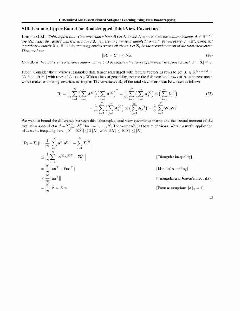
S10. Lemma: Upper Bound for Bootstrapped Total-View CovarianceLemma S10.1. (Subsampled total-view covariance bound) Let X be the N ×m× d tensor whose elements A ∈ Rm×dare identically distributed matrices with rows Ai representing m-views sampled from a larger set of views in Rd. Constructa total-view matrix X ∈ Rm×d by summing entries across all views. Let Σt be the second moment of the total-view space.Then, we have

‖Rt −Σt‖ ≤ Nm (26)

Here Rt is the total-view covariance matrix and c2 > 0 depends on the range of the total view space k such that |X| ≤ k.

Proof. Consider the m-view subsampled data tensor rearranged with feature vectors as rows to get X ∈ RN×m×d =[A(1), ...,A(N)] with rows of A∗ as Ai. Without loss of generality, assume the d-dimensional rows of A to be zero meanwhich makes estimating covariances simpler. The covariance Rt of the total view matrix can be written as follows

Rt =1

m

N∑i=1

( m∑i=1

A(i))( m∑

i=1

A(i))>

=1

m

N∑i=1

( m∑j=1

A(i)j

)⊗( m∑j=1

A(i)j

)(27)

=1

m

N∑i=1

( m∑j=1

A(i)j

)⊗( m∑j=1

A(i)j

)=

1

m

N∑i=1

WiW>i

We want to bound the difference between this subsampled total-view covariance matrix and the second moment of thetotal-view space. Let a(i) =

∑mj=1 A

(i)j for i = 1, . . . , N . The vector a(i) is the sum-of-views. We use a useful application

of Jensen’s inequality here: ‖X − EX‖ ≤ 2‖X‖ with |EX| ≤ E|X| ≤ |X|

‖Rt −Σt‖ =1

m

∥∥∥∥∥N∑i=1

a(i)a(i)> −N∑i=1

Σ(i)t

∥∥∥∥∥≤ 1

m

N∑i=1

∥∥∥a(i)a(i)> −Σ(i)t

∥∥∥ [Triangular inequality]

=N

m

∥∥aa> − Eaa>∥∥ [Identical sampling]

≤ N

m

∥∥aa>∥∥ [Triangular and Jensen’s inequality]

=N

mm2 = Nm [From assumption: ‖a‖2 = 1]


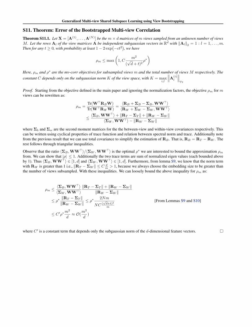
S11. Theorem: Error of the Bootstrapped Multi-view CorrelationTheorem S11.1. Let X = [A(1), . . . ,A(N)] be the m× d matrices of m views sampled from an unknown number of viewsM . Let the rows Al of the view matrices A be independent subgaussian vectors in Rd with ‖Al‖2 = 1 : l = 1, . . . ,m.Then for any t ≥ 0, with probability at least 1− 2 exp

(−ct2

), we have

ρm ≤ max

(1, C

m2

(√d+ t)2

ρ∗)

Here, ρm and ρ∗ are the mv-corr objectives for subsampled views m and the total number of views M respectively. Theconstant C depends only on the subgaussian norm K of the view space, with K = max

i,l

∥∥∥A(i)l

∥∥∥ψ2

Proof. Starting from the objective defined in the main paper and ignoring the normalization factors, the objective ρm for mviews can be rewritten as:

ρm =Tr(W>RBW)

Tr(W>RWW)=〈RB + ΣB −ΣB ,WW>〉〈RW + ΣW −ΣW ,WW>〉

≤ 〈ΣB ,WW>〉+ ‖RT −ΣT ‖+ ‖RW −ΣW ‖〈ΣW ,WW>〉 − ‖RW −ΣW ‖

where Σb and Σw are the second moment matrices for the the between-view and within-view covariances respectively. Thiscan be written using cyclical properties of trace function and relation between spectral norm and trace. Additionally notefrom the previous result that we can use total covariance to simplify the estimation of RB . That is, RB = RT −RW . Therest follows through triangular inequalities.

Observe that the ratio 〈ΣB ,WW>〉/〈ΣW ,WW>〉 is the optimal ρ∗ we are interested to bound the approximation ρmfrom. We can show that |ρ| ≤ 1. Additionally the two trace terms are sum of normalized eigen values (each bounded aboveby 1). Thus 〈ΣB ,WW>〉 ∈ [1, d] and 〈ΣW ,WW>〉 ∈ [1, d]. Furthermore, from lemma S9, we know that the norm termwith RW is greater than 1 i.e., ‖RT −ΣW ‖ ≤ C d

m > 1, because we always choose the embedding size to be greater thanthe number of views subsampled. With these inequalities. We can loosely bound the above inequality for ρm as:

ρm ≤〈ΣB ,WW>〉〈ΣW ,WW>〉

‖RT −ΣT ‖+ ‖RW −ΣW ‖‖RW −ΣW ‖

≤ ρ∗ ‖RT −ΣT ‖‖RW −ΣW ‖

≤ ρ∗ 2Nm

NC (√d+t)2

m

[From Lemmas S9 and S10]

≤ C ′ρ∗m2

d≈ O(

m2

d)

where C ′ is a constant term that depends only the subgaussian norm of the d-dimensional feature vectors.


ReferencesAndrew, G., Arora, R., Bilmes, J., and Livescu, K. Deep canonical correlation analysis. In International Conference on

Machine Learning, pp. 1247–1255, 2013.

Bartko, J. J. The intraclass correlation coefficient as a measure of reliability. Psychological reports, 19(1):3–11, 1966.

Benton, A., Khayrallah, H., Gujral, B., Reisinger, D. A., Zhang, S., and Arora, R. Deep generalized canonical correlationanalysis. arXiv preprint arXiv:1702.02519, 2017.

Cai, X., Wang, C., Xiao, B., Chen, X., and Zhou, J. Regularized latent least square regression for cross pose face recognition.In Twenty-Third international joint conference on Artificial Intelligence, 2013.

Chatfield, K., Simonyan, K., Vedaldi, A., and Zisserman, A. Return of the devil in the details: Delving deep intoconvolutional nets. arXiv preprint arXiv:1405.3531, 2014.

Chaudhuri, K., Kakade, S. M., Livescu, K., and Sridharan, K. Multi-view clustering via canonical correlation analysis. InProceedings of the 26th annual international conference on machine learning, pp. 129–136, 2009.

Dehak, N., Kenny, P., Dehak, R., Glembek, O., Dumouchel, P., Burget, L., Hubeika, V., and Castaldo, F. Support vectormachines and joint factor analysis for speaker verification. In 2009 IEEE International Conference on Acoustics, Speechand Signal Processing, pp. 4237–4240. IEEE, 2009.

Dehak, N., Kenny, P. J., Dehak, R., Dumouchel, P., and Ouellet, P. Front-end factor analysis for speaker verification. IEEETransactions on Audio, Speech, and Language Processing, 19(4):788–798, 2011.

Ding, Z. and Fu, Y. Low-rank common subspace for multi-view learning. In 2014 IEEE international conference on DataMining, pp. 110–119. IEEE, 2014.

Ding, Z. and Fu, Y. Robust multiview data analysis through collective low-rank subspace. IEEE transactions on neuralnetworks and learning systems, 29(5):1986–1997, 2017.

Ding, Z., Shao, M., and Fu, Y. Robust multi-view representation: A unified perspective from multi-view learning to domainadaption. In IJCAI, pp. 5434–5440, 2018.

Dorfer, M., Kelz, R., and Widmer, G. Deep linear discriminant analysis. arXiv preprint arXiv:1511.04707, 2015.

Dorfer, M., Schluter, J., Vall, A., Korzeniowski, F., and Widmer, G. End-to-end cross-modality retrieval with cca projectionsand pairwise ranking loss. International Journal of Multimedia Information Retrieval, 7(2):117–128, 2018.

Dumpala, S. H., Sheikh, I., Chakraborty, R., and Kopparapu, S. K. Sentiment classification on erroneous asr transcripts: Amulti view learning approach. In 2018 IEEE Spoken Language Technology Workshop (SLT), pp. 807–814. IEEE, 2018.

Feng, Y., You, H., Zhang, Z., Ji, R., and Gao, Y. Hypergraph neural networks. In Proceedings of the AAAI Conference onArtificial Intelligence, volume 33, pp. 3558–3565, 2019.

Fisher, R. A. The use of multiple measurements in taxonomic problems. Annals of eugenics, 7(2):179–188, 1936.

Ganin, Y., Ustinova, E., Ajakan, H., Germain, P., Larochelle, H., Laviolette, F., Marchand, M., and Lempitsky, V. Domain-adversarial training of neural networks. The Journal of Machine Learning Research, 17(1):2096–2030, 2016.

Gross, R., Matthews, I., Cohn, J., Kanade, T., and Baker, S. Multi-pie. Image and Vision Computing, 28(5):807–813, 2010.

Horst, P. Generalized canonical correlations and their applications to experimental data. Journal of Clinical Psychology, 17(4):331–347, 1961.

Hotelling, H. Relations between two sets of variates. In Breakthroughs in statistics, pp. 162–190. Springer, 1992.

Jiang, J., Bao, D., Chen, Z., Zhao, X., and Gao, Y. Mlvcnn: Multi-loop-view convolutional neural network for 3d shaperetrieval. In Proceedings of the AAAI Conference on Artificial Intelligence, volume 33, pp. 8513–8520, 2019.


Kan, M., Shan, S., Zhang, H., Lao, S., and Chen, X. Multi-view discriminant analysis. IEEE transactions on patternanalysis and machine intelligence, 38(1):188–194, 2015.

Kan, M., Shan, S., and Chen, X. Multi-view deep network for cross-view classification. In Proceedings of the IEEEConference on Computer Vision and Pattern Recognition, pp. 4847–4855, 2016.

Kepuska, V. and Klein, T. A novel wake-up-word speech recognition system, wake-up-word recognition task, technologyand evaluation. Nonlinear Analysis: Theory, Methods & Applications, 71(12):e2772–e2789, 2009.

Khan, S. H., Guo, Y., Hayat, M., and Barnes, N. Unsupervised primitive discovery for improved 3d generative modeling. InProceedings of the IEEE Conference on Computer Vision and Pattern Recognition, pp. 9739–9748, 2019.

Klemen, J. and Chambers, C. D. Current perspectives and methods in studying neural mechanisms of multisensoryinteractions. Neuroscience & Biobehavioral Reviews, 36(1):111–133, 2012.

Ledoit, O. and Wolf, M. A well-conditioned estimator for large-dimensional covariance matrices. Journal of MultivariateAnalysis, 88(2):365411, Feb 2004.

Li, Y. et al. A survey of multi-view representation learning. IEEE Transactions on Knowledge and Data Engineering, 2018.

Parra, L. C., Haufe, S., and Dmochowski, J. P. Correlated components analysis: Extracting reliable dimensions in multivariatedata. stat, 1050:26, 2018.

Pedregosa, F., Varoquaux, G., Gramfort, A., Michel, V., Thirion, B., Grisel, O., Blondel, M., Prettenhofer, P., Weiss, R.,Dubourg, V., Vanderplas, J., Passos, A., Cournapeau, D., Brucher, M., Perrot, M., and Duchesnay, E. Scikit-learn:Machine learning in Python. Journal of Machine Learning Research, 12:2825–2830, 2011.

Shankar, S., Piratla, V., Chakrabarti, S., Chaudhuri, S., Jyothi, P., and Sarawagi, S. Generalizing across domains viacross-gradient training. arXiv preprint arXiv:1804.10745, 2018.

Sharma, A., Kumar, A., Daume, H., and Jacobs, D. W. Generalized multiview analysis: A discriminative latent space. InComputer Vision and Pattern Recognition (CVPR), 2012 IEEE Conference on, pp. 2160–2167. IEEE, 2012.

Snyder, D., Garcia-Romero, D., Povey, D., and Khudanpur, S. Deep neural network embeddings for text-independentspeaker verification. In Interspeech, pp. 999–1003, 2017.

Soltanolkotabi, M., Elhamifar, E., Candes, E. J., et al. Robust subspace clustering. The Annals of Statistics, 42(2):669–699,2014.

Somandepalli, K., Kelly, C., Reiss, . E., Castellanos, F. X., Milham, M. P., and Di Martino, A. Short-term test–retestreliability of resting state fmri metrics in children with and without attention-deficit/hyperactivity disorder. DevelopmentalCognitive Neuroscience, 15:83–93, 2015.

Somandepalli, K., Kumar, N., Jati, A., Georgiou, P., and Narayanan, S. Multiview shared subspace learning across speakersand speech commands. Proc. Interspeech 2019, pp. 2320–2324, 2019a.

Somandepalli, K., Kumar, N., Travadi, R., and Narayanan, S. Multimodal representation learning using deep multisetcanonical correlation, 2019b.

Su, H., Maji, S., Kalogerakis, E., and Learned-Miller, E. Multi-view convolutional neural networks for 3d shape recognition.In Proceedings of the IEEE international conference on computer vision, pp. 945–953, 2015.

Sun, S., Liu, Y., and Mao, L. Multi-view learning for visual violence recognition with maximum entropy discrimination anddeep features. Information Fusion, 50:43–53, 2019.

Vershynin, R. Introduction to the non-asymptotic analysis of random matrices. arXiv preprint arXiv:1011.3027, 2010.

Wang, F., Chen, L., Li, C., Huang, S., Chen, Y., Qian, C., and Change Loy, C. The devil of face recognition is in the noise.In Proceedings of the European Conference on Computer Vision (ECCV), pp. 765–780, 2018.

Wang, W., Arora, R., Livescu, K., and Bilmes, J. On deep multi-view representation learning. In International Conferenceon Machine Learning, pp. 1083–1092, 2015.


Warden, P. Speech commands: A dataset for limited-vocabulary speech recognition. CoRR, abs/1804.03209, 2018.

Wu, Z., Song, S., Khosla, A., Yu, F., Zhang, L., Tang, X., and Xiao, J. 3d shapenets: A deep representation for volumetricshapes. In Proceedings of the IEEE conference on computer vision and pattern recognition, pp. 1912–1920, 2015.

Xu, C., Tao, D., and Xu, C. A survey on multi-view learning. arXiv preprint arXiv:1304.5634, 2013.

Zhao, J., Xie, X., Xu, X., and Sun, S. Multi-view learning overview. Inf. Fusion, 38(C):43–54, November 2017. ISSN1566-2535. doi: 10.1016/j.inffus.2017.02.007.

Documents

Generalized Multi-view Shared Subspace Learning using View