Embed Size (px)
Citation preview
GENERALIZED HARISH-CHANDRA DESCENT, GELFAND PAIRS AND ANARCHIMEDEAN ANALOG OF JACQUET-RALLIS’ THEOREM
AVRAHAM AIZENBUD AND DMITRY GOUREVITCH
with Appendix D by Avraham Aizenbud, Dmitry Gourevitch and Eitan Sayag
Abstract. In the first part of the paper we generalize a descent technique due to Harish-Chandra to
the case of a reductive group acting on a smooth affine variety both defined over an arbitrary local fieldF of characteristic zero. Our main tool is the Luna Slice Theorem.
In the second part of the paper we apply this technique to symmetric pairs. In particular we prove
that the pairs (GLn+k(F ), GLn(F ) × GLk(F )) and (GLn(E), GLn(F )) are Gelfand pairs for any localfield F and its quadratic extension E. In the non-Archimedean case, the first result was proven earlier
by Jacquet and Rallis and the second by Flicker.
We also prove that any conjugation invariant distribution on GLn(F ) is invariant with respect totransposition. For non-Archimedean F the latter is a classical theorem of Gelfand and Kazhdan.
Contents
1. Introduction 21.1. Main results 21.2. Related work 31.3. Structure of the paper 31.4. Acknowledgements 4
Part 1. Generalized Harish-Chadra descent 42. Preliminaries and notation 42.1. Conventions 42.2. Categorical quotient 52.3. Algebraic geometry over local fields 52.4. Vector systems 72.5. Distributions 73. Generalized Harish-Chandra descent 93.1. Generalized Harish-Chandra descent 93.2. A stronger version 104. Distributions versus Schwartz distributions 125. Applications of Fourier transform and the Weil representation 125.1. Preliminaries 135.2. Applications 136. Tame actions 14
Part 2. Symmetric and Gelfand pairs 157. Symmetric pairs 157.1. Preliminaries and notation 167.2. Descendants of symmetric pairs 177.3. Tame symmetric pairs 18
Key words and phrases. Multiplicity one, Gelfand pairs, symmetric pairs, Luna Slice Theorem, invariant distributions,Harish-Chandra descent, uniqueness of linear periods.
MSC Classes: 20C99, 20G05, 22E45, 22E50, 46F10, 14L24, 14L30.
1
2 AVRAHAM AIZENBUD AND DMITRY GOUREVITCH
7.4. Regular symmetric pairs 197.5. Conjectures 217.6. The pairs (G×G,∆G) and (GE/F , G) are tame 217.7. The pair (GLn+k,GLn ×GLk) is a GK pair. 228. Applications to Gelfand pairs 248.1. Preliminaries on Gelfand pairs and distributional criteria 248.2. Applications to Gelfand pairs 25
Part 3. Appendices 25Appendix A. Algebraic geometry over local fields 25A.1. Implicit Function Theorems 25A.2. The Luna Slice Theorem 26Appendix B. Schwartz distributions on Nash manifolds 26B.1. Preliminaries and notation 26B.2. Submersion principle 27B.3. Frobenius reciprocity 28B.4. K-invariant distributions compactly supported modulo K. 29Appendix C. Proof of the Archimedean Homogeneity Theorem 30Appendix D. Localization Principle 31Appendix E. Diagram 33References 34
1. Introduction
Harish-Chandra developed a technique based on Jordan decomposition that allows to reduce certainstatements on conjugation invariant distributions on a reductive group to the set of unipotent elements,provided that the statement is known for certain subgroups (see e.g. [HC99]).
In this paper we generalize an aspect of this technique to the setting of a reductive group acting on asmooth affine algebraic variety, using the Luna Slice Theorem. Our technique is oriented towards provingGelfand property for pairs of reductive groups.
Our approach is uniform for all local fields of characteristic zero – both Archimedean and non-Archimedean.
1.1. Main results.The core of this paper is Theorem 3.1.1:
Theorem. Let a reductive group G act on a smooth affine variety X, both defined over a local field F ofcharacteristic zero. Let χ be a character of G(F ).
Suppose that for any x ∈ X(F ) with closed orbit there are no non-zero distributions on the normalspace at x to the orbit G(F )x which are (G(F )x, χ)-equivariant, where Gx denotes the stabilizer of x.
Then there are no non-zero (G(F ), χ)-equivariant distributions on X(F ).
In fact, a stronger version based on this theorem is given in Corollary 3.2.2. This stronger versionis based on an inductive argument. It shows that it is enough to prove that there are no non-zeroequivariant distributions on the normal space to the orbit G(F )x at x under the assumption that all suchdistributions are supported in a certain closed subset which is the analog of the nilpotent cone.
We apply this stronger version to problems of the following type. Let a reductive group G act on asmooth affine variety X, and τ be an involution of X which normalizes the image of G in Aut(X). Wewant to check whether any G(F )-invariant distribution on X(F ) is also τ -invariant. Evidently, there isthe following necessary condition on τ :(*) Any closed orbit in X(F ) is τ -invariant.In some cases this condition is also sufficient. In these cases we call the action of G on X tame.
GENERALIZED HARISH-CHANDRA DESCENT 3
This is a weakening of the property called ”density” in [RR96]. However, it is sufficient for the purposeof proving Gelfand property for pairs of reductive groups.
In §6 we give criteria for tameness of actions. In particular, we introduce the notion of ”special” actionin order to show that certain actions are tame (see Theorem 6.0.5 and Proposition 7.3.5). Also, in manycases one can verify that an action is special using purely algebraic-geometric means.
In the second part of the paper we restrict our attention to the case of symmetric pairs. We transferthe terminology on actions to terminology on symmetric pairs. For example, we call a symmetric pair(G,H) tame if the action of H ×H on G is tame.
In addition we introduce the notion of a ”regular” symmetric pair (see Definition 7.4.2), which alsohelps to prove Gelfand property. Namely, we prove Theorem 7.4.5.
Theorem. Let G be a reductive group defined over a local field F and let θ be an involution of G. LetH := Gθ and let σ be the anti-involution defined by σ(g) := θ(g−1). Consider the symmetric pair (G,H).
Suppose that all its ”descendants” (including itself, see Definition 7.2.2) are regular. Suppose also thatany closed H(F )-double coset in G(F ) is σ-invariant.
Then every bi-H(F )-invariant distribution on G(F ) is σ-invariant. In particular, by Gelfand-Kazhdancriterion, the pair (G,H) is a Gelfand pair (see §8).
Also, we formulate an algebraic-geometric criterion for regularity of a pair (Proposition 7.3.7). Wesum up the various properties of symmetric pairs and their interrelations in a diagram in Appendix E.
As an application and illustration of our methods we prove in §7.7 that the pair (GLn+k,GLn×GLk)is a Gelfand pair by proving that it is regular, along with its descendants. In the non-Archimedean casethis was proven in [JR96] and our proof is along the same lines. Our technique enabled us to streamlinesome of the computations in the proof of [JR96] and to extend it to the Archimedean case.
We also prove (in §7.6) that the pair (G(E), G(F )) is tame for any reductive group G over F and aquadratic field extension E/F . This implies that the pair (GLn(E),GLn(F )) is a Gelfand pair. In thenon-Archimedean case this was proven in [Fli91]. Also we prove that the adjoint action of a reductivegroup on itself is tame. This is a generalization of a classical theorem by Gelfand and Kazhdan, see[GK75].
In general, we conjecture that any symmetric pair is regular. This would imply the van Dijk conjecture:
Conjecture (van Dijk). Any symmetric pair (G,H) over C such that G/H is connected is a Gelfandpair.
1.2. Related work.This paper was inspired by the paper [JR96] by Jacquet and Rallis where they prove that the pair(GLn+k(F ),GLn(F )×GLk(F )) is a Gelfand pair for any non-Archimedean local field F of characteristiczero. Our aim was to see to what extent their techniques generalize.
Another generalization of Harish-Chandra descent using the Luna Slice Theorem has been carried outin the non-Archimedean case in [RR96]. In that paper Rader and Rallis investigated spherical charactersof H-distinguished representations of G for symmetric pairs (G,H) and checked the validity of what theycall the ”density principle” for rank one symmetric pairs. They found out that the principle usuallyholds, but also found counterexamples.
In [vD86], van-Dijk investigated rank one symmetric pairs in the Archimedean case and classified theGelfand pairs among them. In [BvD94], van-Dijk and Bosman studied the non-Archimedean case andobtained results for most rank one symmetric pairs. We hope that the second part of our paper willenhance the understanding of this question for symmetric pairs of higher rank.
1.3. Structure of the paper.In §2 we introduce notation and terminology which allows us to speak uniformly about spaces of pointsof smooth algebraic varieties over Archimedean and non-Archimedean local fields, and equivariant distri-butions on those spaces.
In §§2.3 we formulate a version of the Luna Slice Theorem for points over local fields (Theorem 2.3.17).In §§2.5 we formulate results on equivariant distributions and equivariant Schwartz distributions. Mostof those results are borrowed from [BZ76], [Ber84], [Bar03] and [AGS08], and the rest are proven inAppendix B.
4 AVRAHAM AIZENBUD AND DMITRY GOUREVITCH
In §3 we formulate and prove the Generalized Harish-Chandra Descent Theorem and its strongerversion.§4 is of interest only in the Archimedean case. In that section we prove that in the cases at hand if
there are no equivariant Schwartz distributions then there are no equivariant distributions at all. Schwartzdistributions are discussed in Appendix B.
In §5 we formulate a homogeneity Theorem which helps us to check the conditions of the GeneralizedHarish-Chandra Descent Theorem. In the non-Archimedean case this theorem had been proved earlier(see e.g. [JR96], [RS07] or [AGRS07]). We provide the proof for the Archimedean case in Appendix C.
In §6 we introduce the notion of tame actions and provide tameness criteria.In §7 we apply our tools to symmetric pairs. In §§7.3 we provide criteria for tameness of a symmetric
pair. In §§7.4 we introduce the notion of a regular symmetric pair and prove Theorem 7.4.5 alludedto above. In §§7.5 we discuss conjectures about the regularity and the Gelfand property of symmet-ric pairs. In §§7.6 we prove that certain symmetric pairs are tame. In §§7.7 we prove that the pair(GLn+k(F ),GLn(F )×GLk(F )) is regular.
In §8 we recall basic facts on Gelfand pairs and their connections to invariant distributions. We alsoprove that the pairs (GLn+k(F ),GLn(F ) × GLk(F )) and (GLn(E),GLn(F )) are Gelfand pairs for anylocal field F and its quadratic extension E.
We start Appendix A by discussing different versions of the Inverse Function Theorem for local fields.Then we prove a version of the Luna Slice Theorem for points over local fields (Theorem 2.3.17). ForArchimedean F this was done by Luna himself in [Lun75].
Appendices B and C are of interest only in the Archimedean case.In Appendix B we discuss Schwartz distributions on Nash manifolds. We prove Frobenius reciprocity
for them and construct the pullback of a Schwartz distribution under a Nash submersion. Also weprove that G-invariant distributions which are (Nashly) compactly supported modulo G are Schwartzdistributions.
In Appendix C we prove the Archimedean version of the Homogeneity Theorem discussed in §5.In Appendix D we formulate and prove a version of Bernstein’s Localization Principle (Theorem
4.0.1). This appendix is of interest only for Archimedean F since for l-spaces a more general version ofthis principle had been proven in [Ber84]. This appendix is used in §4.
In [AGS09] we formulated Localization Principle in the setting of differential geometry. Admittedly,we currently do not have a proof of this principle in such a general setting. However, in Appendix D wepresent a proof in the case of a reductive group G acting on a smooth affine variety X. This generality issufficiently wide for all applications we encountered up to now, including the one considered in [AGS09].
Finally, in Appendix E we present a diagram that illustrates the interrelations of various properties ofsymmetric pairs.
1.4. Acknowledgements. We would like to thank our teacher Joseph Bernstein for our mathematicaleducation.
We also thank Vladimir Berkovich, Joseph Bernstein, Gerrit van Dijk, Stephen Gelbart,Maria Gorelik, Herve Jacquet, David Kazhdan, Erez Lapid, Shifra Reif, Eitan Sayag, DavidSoudry, Yakov Varshavsky and Oksana Yakimova for fruitful discussions, and Sun Binyong andthe referees for useful remarks.
Finally we thank Anna Gourevitch for the graphical design of Appendix E.Both authors are partially supported by BSF grant, GIF grant, and ISF Center of excellency grant.
Part 1. Generalized Harish-Chadra descent
2. Preliminaries and notation
2.1. Conventions.• Henceforth we fix a local field F of characteristic zero. All the algebraic varieties and algebraic
groups that we will consider will be defined over F .• For a group G acting on a set X we denote by XG the set of fixed points of X. Also, for an
element x ∈ X we denote by Gx the stabilizer of x.
GENERALIZED HARISH-CHANDRA DESCENT 5
• By a reductive group we mean a (non-necessarily connected) algebraic reductive group.• We consider an algebraic variety X defined over F as an algebraic variety over F together with
action of the Galois group Gal(F/F ). On X we only consider the Zariski topology. On X(F ) weonly consider the analytic (Hausdorff) topology. We treat finite-dimensional linear spaces definedover F as algebraic varieties.
• The tangent space of a manifold (algebraic, analytic, etc.) X at x will be denoted by TxX.• Usually we will use the letters X,Y, Z,∆ to denote algebraic varieties and the letters G,H to
denote reductive groups. We will usually use the letters V,W,U,K,M,N,C,O, S, T to denoteanalytic spaces (such as F -points of algebraic varieties) and the letter K to denote analyticgroups. Also we will use the letters L, V,W to denote vector spaces of all kinds.
2.2. Categorical quotient.
Definition 2.2.1. Let an algebraic group G act on an algebraic variety X. A pair consisting of analgebraic variety Y and a G-invariant morphism π : X → Y is called the quotient of X by the actionof G if for any pair (π′, Y ′), there exists a unique morphism φ : Y → Y ′ such that π′ = φ π. Clearly,if such pair exists it is unique up to a canonical isomorphism. We will denote it by (πX , X/G).
Theorem 2.2.2 (cf. [Dre00]). Let a reductive group G act on an affine variety X. Then the quotientX/G exists, and every fiber of the quotient map πX contains a unique closed orbit. In fact, X/G :=SpecO(X)G.
2.3. Algebraic geometry over local fields.
2.3.1. Analytic manifolds.In this paper we consider distributions over l-spaces, smooth manifolds and Nash manifolds. l-spaces arelocally compact totally disconnected topological spaces and Nash manifolds are semi-algebraic smoothmanifolds.
For basic facts on l-spaces and distributions over them we refer the reader to [BZ76, §1].For basic facts on Nash manifolds and Schwartz functions and distributions over them see Appendix
B and [AG08a]. In this paper we consider only separated Nash manifolds.We now introduce notation and terminology which allows a uniform treatment of the Archimedean
and the non-Archimedean cases.We will use the notion of an analytic manifold over a local field (see e.g. [Ser64, Part II, Chapter III]).
When we say ”analytic manifold” we always mean analytic manifold over some local field. Note thatan analytic manifold over a non-Archimedean field is in particular an l-space and an analytic manifoldover an Archimedean field is in particular a smooth manifold.
Definition 2.3.1. A B-analytic manifold is either an analytic manifold over a non-Archimedean localfield, or a Nash manifold.
Remark 2.3.2. If X is a smooth algebraic variety, then X(F ) is a B-analytic manifold and (TxX)(F ) =Tx(X(F )).
Notation 2.3.3. Let M be an analytic manifold and S be an analytic submanifold. We denote by NMS :=
(TM |Y )/TS the normal bundle to S in M . The conormal bundle is defined by CNMS := (NM
S )∗.Denote by Symk(CNM
S ) the k-th symmetric power of the conormal bundle. For a point y ∈ S we denoteby NM
S,y the normal space to S in M at the point y and by CNMS,y the conormal space.
2.3.2. G-orbits on X and G(F )-orbits on X(F ).
Lemma 2.3.4 (see Appendix A.1). Let G be an algebraic group and let H ⊂ G be a closed subgroup.Then G(F )/H(F ) is open and closed in (G/H)(F ).
Corollary 2.3.5. Let an algebraic group G act on an algebraic variety X. Let x ∈ X(F ). Then
NXGx,x(F ) ∼= N
X(F )G(F )x,x.

6 AVRAHAM AIZENBUD AND DMITRY GOUREVITCH
Proposition 2.3.6. Let an algebraic group G act on an algebraic variety X. Suppose that S ⊂ X(F ) isa non-empty closed G(F )-invariant subset. Then S contains a closed orbit.
Proof. The proof is by Noetherian induction on X. Choose x ∈ S. Consider Z := Gx−Gx.If Z(F )∩S is empty then Gx(F )∩S is closed and hence G(F )x∩S is closed by Lemma 2.3.4. Therefore
G(F )x is closed.If Z(F ) ∩ S is non-empty then Z(F ) ∩ S contains a closed orbit by the induction assumption.
Corollary 2.3.7. Let an algebraic group G act on an algebraic variety X. Let U be an open G(F )-invariant subset of X(F ). Suppose that U contains all closed G(F )-orbits. Then U = X(F ).
Theorem 2.3.8 ([RR96], §2 fact A, pages 108-109). Let a reductive group G act on an affine variety X.Let x ∈ X(F ). Then the following are equivalent:(i) G(F )x ⊂ X(F ) is closed (in the analytic topology).(ii) Gx ⊂ X is closed (in the Zariski topology).
Definition 2.3.9. Let a reductive group G act on an affine variety X. We call an element x ∈ XG-semisimple if its orbit Gx is closed.
In particular, in the case where G acts on itself by conjugation, the notion of G-semisimplicity coincideswith the usual one.
Notation 2.3.10. Let V be an F -rational finite-dimensional representation of a reductive group G. Weset
QG(V ) := Q(V ) := (V/V G)(F ).Since G is reductive, there is a canonical embedding Q(V ) → V (F ). Let π : V (F ) → (V/G)(F ) be thenatural map. We set
ΓG(V ) := Γ(V ) := π−1(π(0)).Note that Γ(V ) ⊂ Q(V ). We also set
RG(V ) := R(V ) := Q(V )− Γ(V ).
Notation 2.3.11. Let a reductive group G act on an affine variety X. For a G-semisimple elementx ∈ X(F ) we set
Sx := y ∈ X(F ) |G(F )y 3 x.
Lemma 2.3.12. Let V be an F -rational finite-dimensional representation of a reductive group G. ThenΓ(V ) = S0.
This lemma follows from [RR96, fact A on page 108] for non-Archimedean F and [Brk71, Theorem5.2 on page 459] for Archimedean F .
Example 2.3.13. Let a reductive group G act on its Lie algebra g by the adjoint action. Then Γ(g) isthe set of nilpotent elements of g.
Proposition 2.3.14. Let a reductive group G act on an affine variety X. Let x, z ∈ X(F ) be G-semisimple elements which do not lie in the same orbit of G(F ). Then there exist disjoint G(F )-invariantopen neighborhoods Ux of x and Uz of z.
For the proof of this Proposition see [Lun75] for Archimedean F and [RR96, fact B on page 109] fornon-Archimedean F .
Corollary 2.3.15. Let a reductive group G act on an affine variety X. Suppose that x ∈ X(F ) is aG-semisimple element. Then the set Sx is closed.
Proof. Let y ∈ Sx. By Proposition 2.3.6, G(F )y contains a closed orbit G(F )z. If G(F )z = G(F )xthen y ∈ Sx. Otherwise, choose disjoint open G-invariant neighborhoods Uz of z and Ux of x. Sincez ∈ G(F )y, Uz intersects G(F )y and hence contains y. Since y ∈ Sx, this means that Uz intersects Sx.Let t ∈ Uz ∩ Sx. Since Uz is G(F )-invariant, G(F )t ⊂ Uz. By the definition of Sx, x ∈ G(F )t and hencex ∈ Uz. Hence Uz intersects Ux – contradiction!

GENERALIZED HARISH-CHANDRA DESCENT 7
2.3.3. Analytic Luna slices.
Definition 2.3.16. Let a reductive group G act on an affine variety X. Let π : X(F ) → (X/G)(F ) be thenatural map. An open subset U ⊂ X(F ) is called saturated if there exists an open subset V ⊂ (X/G)(F )such that U = π−1(V ).
We will use the following corollary of the Luna Slice Theorem:
Theorem 2.3.17 (see Appendix A.2). Let a reductive group G act on a smooth affine variety X. Letx ∈ X(F ) be G-semisimple. Consider the natural action of the stabilizer Gx on the normal space NX
Gx,x.Then there exist(i) an open G(F )-invariant B-analytic neighborhood U of G(F )x in X(F ) with a G-equivariant B-analyticretract p : U → G(F )x and(ii) a Gx-equivariant B-analytic embedding ψ : p−1(x) → NX
Gx,x(F ) with an open saturated image suchthat ψ(x) = 0.
Definition 2.3.18. In the notation of the previous theorem, denote S := p−1(x) and N := NXGx,x(F ).
We call the quintuple (U, p, ψ, S,N) an analytic Luna slice at x.
Corollary 2.3.19. In the notation of the previous theorem, let y ∈ p−1(x). Denote z := ψ(y). Then(i) (G(F )x)z = G(F )y(ii) NX(F )
G(F )y,y∼= NN
G(F )xz,zas G(F )y-spaces
(iii) y is G-semisimple if and only if z is Gx-semisimple.
2.4. Vector systems. 1
In this subsection we introduce the term ”vector system”. This term allows to formulate statementsin wider generality.
Definition 2.4.1. For an analytic manifold M we define the notions of a vector system and a B-vectorsystem over it.
For a smooth manifold M , a vector system over M is a pair (E,B) where B is a smooth locally trivialfibration over M and E is a smooth (finite-dimensional) vector bundle over B.
For a Nash manifold M , a B-vector system over M is a pair (E,B) where B is a Nash fibration overM and E is a Nash (finite-dimensional) vector bundle over B.
For an l-space M , a vector system over M (or a B-vector system over M) is a sheaf of complex linearspaces.
In particular, in the case where M is a point, a vector system over M is either a C-vector spaceif F is non-Archimedean, or a smooth manifold together with a vector bundle in the case where F isArchimedean. The simplest example of a vector system over a manifold M is given by the following.
Definition 2.4.2. Let V be a vector system over a point pt. Let M be an analytic manifold. A constantvector system with fiber V is the pullback of V with respect to the map M → pt. We denote it by VM .
2.5. Distributions.
Definition 2.5.1. Let M be an analytic manifold over F . We define C∞c (M) in the following way.If F is non-Archimedean then C∞c (M) is the space of locally constant compactly supported complex
valued functions on M . We do not consider any topology on C∞c (M).If F is Archimedean then C∞c (M) is the space of smooth compactly supported complex valued functions
on M , endowed with the standard topology.For any analytic manifold M , we define the space of distributions D(M) by D(M) := C∞c (M)∗. We
consider the weak topology on it.
1Subsection 2.4 and in particular the notion of ”vector system” along with the results at the end of §§3.1 and §§3.2 are
not essential for the rest of the paper. They are merely included for future reference.
8 AVRAHAM AIZENBUD AND DMITRY GOUREVITCH
Definition 2.5.2. Let M be a B-analytic manifold. We define S(M) in the following way.If M is an analytic manifold over non-Archimedean field, S(M) := C∞c (M).If M is a Nash manifold, S(M) is the space of Schwartz functions on M , namely smooth functions
which are rapidly decreasing together with all their derivatives. See [AG08a] for the precise definition.We consider S(M) as a Frechet space.
For any B-analytic manifold M , we define the space of Schwartz distributions S∗(M) by S∗(M) :=S(M)∗. Clearly, S(M)∗ is naturally embedded into D(M).
Notation 2.5.3. Let M be an analytic manifold. For a distribution ξ ∈ D(M) we denote by Supp(ξ)the support of ξ.
For a closed subset N ⊂M we denote
DM (N) := ξ ∈ D(M)|Supp(ξ) ⊂ N.More generally, for a locally closed subset N ⊂M we denote
DM (N) := DM\(N\N)(N).
Similarly if M is a B-analytic manifold and N is a locally closed subset we define S∗M (N) in a similarvein. 2
Definition 2.5.4. Let M be an analytic manifold over F and E be a vector system over M . We defineC∞c (M, E) in the following way.
If F is non-Archimedean then C∞c (M, E) is the space of compactly supported sections of E.If F is Archimedean and E = (E,B) where B is a fibration over M and E is a vector bundle over B,
then C∞c (M, E) is the complexification of the space of smooth compactly supported sections of E over B.If V is a vector system over a point then we denote C∞c (M,V) := C∞c (M,VM ).
We define D(M, E), DM (N, E), S(M, E), S∗(M, E) and S∗M (N, E) in the natural way.
Theorem 2.5.5. Let an l-group K act on an l-space M . Let M =⋃li=0Mi be a K-invariant stratification
of M . Let χ be a character of K. Suppose that S∗(Mi)K,χ = 0. Then S∗(M)K,χ = 0.
This theorem is a direct corollary of [BZ76, Corollary 1.9].For the proof of the next two theorems see e.g. [AGS08, §7.2].
Theorem 2.5.6 (Bruhat). Let a Lie group K act on a smooth manifold M . Let N be a locally closedsubset. Let N =
⋃li=0Ni be a smooth K-invariant stratification of N . Let χ be a character of K. Suppose
that for any k ∈ Z≥0 and 0 ≤ i ≤ l,
D(Ni,Symk(CNMNi
))K,χ = 0.
Then DM (N)K,χ = 0.
Theorem 2.5.7. Let a Nash group K act on a Nash manifold M . Let N be a locally closed subset. LetN =
⋃li=0Mi be a Nash K-invariant stratification of M . Let χ be a character of K. Suppose that for
any k ∈ Z≥0 and 0 ≤ i ≤ l,S∗(Ni,Symk(CNM
Ni))K,χ = 0.
Then S∗M (N)K,χ = 0.
Theorem 2.5.8 (Frobenius reciprocity). Let an analytic group K act on an analytic manifold M . LetN be an analytic manifold with a transitive action of K. Let φ : M → N be a K-equivariant map.
Let z ∈ N be a point and Mz := φ−1(z) be its fiber. Let Kz be the stabilizer of z in K. Let ∆K and∆Kz be the modular characters of K and Kz.
Let E be a K-equivariant vector system over M . Then(i) there exists a canonical isomorphism
Fr : D(Mz, E|Mz ⊗∆K |Kz ·∆−1Kz
)Kz ∼= D(M, E)K .
2In the Archimedean case, locally closed is considered with respect to the restricted topology – cf. Appendix B.
GENERALIZED HARISH-CHANDRA DESCENT 9
In particular, Fr commutes with restrictions to open sets.(ii) For B-analytic manifolds Fr maps S∗(Mz, E|Mz
⊗∆K |Kz·∆−1
Kz)Kz to S∗(M, E)K .
For the proof of (i) see [Ber84, §§1.5] and [BZ76, §§2.21 - 2.36] for the case of l-spaces and [AGS08,Theorem 4.2.3] or [Bar03] for smooth manifolds. For the proof of (ii) see Appendix B.
We will also use the following straightforward proposition.
Proposition 2.5.9. Let Ki be analytic groups acting on analytic manifolds Mi for i = 1 . . . n. LetΩi ⊂ Ki be analytic subgroups. Let Ei →Mi be Ki-equivariant vector systems. Suppose that
D(Mi, Ei)Ωi = D(Mi, Ei)Ki
for all i. Then
D(∏
Mi,Ei)∏
Ωi = D(∏
Mi,Ei)∏Ki ,
where denotes the external product.Moreover, if Ωi, Ki, Mi and Ei are B-analytic then the analogous statement holds for Schwartz
distributions.
For the proof see e.g. [AGS08, proof of Proposition 3.1.5].
3. Generalized Harish-Chandra descent
3.1. Generalized Harish-Chandra descent.In this subsection we will prove the following theorem.
Theorem 3.1.1. Let a reductive group G act on a smooth affine variety X. Let χ be a character ofG(F ). Suppose that for any G-semisimple x ∈ X(F ) we have
D(NXGx,x(F ))G(F )x,χ = 0.
ThenD(X(F ))G(F ),χ = 0.
Remark 3.1.2. In fact, the converse is also true. We will not prove it since we will not use it.
For the proof of this theorem we will need the following lemma
Lemma 3.1.3. Let a reductive group G act on a smooth affine variety X. Let χ be a character of G(F ).Let U ⊂ X(F ) be an open saturated subset. Suppose that D(X(F ))G(F ),χ = 0. Then D(U)G(F ),χ = 0.
Proof. Consider the quotient X/G. It is an affine algebraic variety. Embed it in an affine space An. Thisdefines a map π : X(F ) → Fn. Since U is saturated, there exists an open subset V ⊂ (X/G)(F ) suchthat U = π−1(V ). Clearly there exists an open subset V ′ ⊂ Fn such that V ′ ∩ (X/G)(F ) = V .
Let ξ ∈ D(U)G(F ),χ. Suppose that ξ is non-zero. Let x ∈ Suppξ and let y := π(x). Let g ∈ C∞c (V ′)be such that g(y) = 1. Consider ξ′ ∈ D(X(F )) defined by ξ′(f) := ξ(f · (g π)). Clearly, Supp(ξ′) ⊂ Uand hence we can interpret ξ′ as an element in D(X(F ))G(F ),χ. Therefore ξ′ = 0. On the other hand,x ∈ Supp(ξ′). Contradiction.
Proof of Theorem 3.1.1. Let x be a G-semisimple element. Let (Ux,px,ψx, Sx,Nx) be an analytic Lunaslice at x.
Let ξ′ = ξ|Ux . Then ξ′ ∈ D(Ux)G(F ),χ. By Frobenius reciprocity it corresponds to ξ′′ ∈ D(Sx)Gx(F ),χ.The distribution ξ′′ corresponds to a distribution ξ′′′ ∈ D(ψx(Sx))Gx(F ),χ.However, by the previous lemma the assumption implies that D(ψx(Sx))Gx(F ),χ = 0. Hence ξ′ = 0.Let S ⊂ X(F ) be the set of all G-semisimple points. Let U =
⋃x∈S Ux. We saw that ξ|U = 0. On the
other hand, U includes all the closed orbits, and hence by Corollary 2.3.7 U = X.
The following generalization of this theorem is proven in the same way.
10 AVRAHAM AIZENBUD AND DMITRY GOUREVITCH
Theorem 3.1.4. Let a reductive group G act on a smooth affine variety X. Let K ⊂ G(F ) be an opensubgroup and let χ be a character of K. Suppose that for any G-semisimple x ∈ X(F ) we have
D(NXGx,x(F ))Kx,χ = 0.
ThenD(X(F ))K,χ = 0.
Now we would like to formulate a slightly more general version of this theorem concerning K-equivariant vector systems. 3
Definition 3.1.5. Let a reductive group G act on a smooth affine variety X. Let K ⊂ G(F ) be an opensubgroup. Let E be a K-equivariant vector system on X(F ). Let x ∈ X(F ) be G-semisimple. Let E ′ bea Kx-equivariant vector system on NX
Gx,x(F ). We say that E and E ′ are compatible if there exists ananalytic Luna slice (U, p, ψ, S,N) such that E|S = ψ∗(E ′).
Note that if E and E ′ are constant with the same fiber then they are compatible.The following theorem is proven in the same way as Theorem 3.1.1.
Theorem 3.1.6. Let a reductive group G act on a smooth affine variety X. Let K ⊂ G(F ) be anopen subgroup and let E be a K-equivariant vector system on X(F ). Suppose that for any G-semisimplex ∈ X(F ) there exists a K-equivariant vector system E ′ on NX
Gx,x(F ), compatible with E such that
D(NXGx,x(F ), E ′)Kx = 0.
ThenD(X(F ), E)K = 0.
If E and E ′ are B-vector systems and K is an open B-analytic subgroup4 of G(F ) then the theorem alsoholds for Schwartz distributions. Namely, if S∗(NX
Gx,x(F ), E ′)Kx = 0 for any x then S∗(X(F ), E)K = 0.The proof is the same.
3.2. A stronger version.In this section we provide means to validate the conditions of Theorems 3.1.1, 3.1.4 and 3.1.6 based onan inductive argument.
More precisely, the goal of this section is to prove the following theorem.
Theorem 3.2.1. Let a reductive group G act on a smooth affine variety X. Let K ⊂ G(F ) be an opensubgroup and let χ be a character of K. Suppose that for any G-semisimple x ∈ X(F ) such that
D(RGx(NX
Gx,x))Kx,χ = 0
we haveD(QGx
(NXGx,x))
Kx,χ = 0.Then for any G-semisimple x ∈ X(F ) we have
D(NXGx,x(F ))Kx,χ = 0.
Together with Theorem 3.1.4, this theorem gives the following corollary.
Corollary 3.2.2. Let a reductive group G act on a smooth affine variety X. Let K ⊂ G(F ) be an opensubgroup and let χ be a character of K. Suppose that for any G-semisimple x ∈ X(F ) such that
D(R(NXGx,x))
Kx,χ = 0
we haveD(Q(NX
Gx,x))Kx,χ = 0.
Then D(X(F ))K,χ = 0.
3Subsection 2.4 and in particular the notion of ”vector system” along with the results at the end of §§3.1 and §§3.2 arenot essential for the rest of the paper. They are merely included for future reference.
4In fact, any open subgroup of a B-analytic group is B-analytic.
GENERALIZED HARISH-CHANDRA DESCENT 11
From now till the end of the section we fix G, X, K and χ. Let us introduce several definitions andnotation.
Notation 3.2.3. Denote• T ⊂ X(F ) the set of all G-semisimple points.• For x, y ∈ T we say that x > y if Gx % Gy.• T0 := x ∈ T | D(Q(NX
Gx,x))Kx,χ = 0 = x ∈ T | D((NX
Gx,x))Kx,χ = 0.
Proof of Theorem 3.2.1. We have to show that T = T0. Assume the contrary.Note that every chain in T with respect to our ordering has a minimum. Hence by Zorn’s lemma every
non-empty set in T has a minimal element. Let x be a minimal element of T −T0. To get a contradiction,it is enough to show that D(R(NX
Gx,x))Kx,χ = 0.
Denote R := R(NXGx,x). By Theorem 3.1.4, it is enough to show that for any y ∈ R we have
D(NRG(F )xy,y
)(Kx)y,χ = 0.
Let (U, p, ψ, S,N) be an analytic Luna slice at x.Since ψ(S) is open and contains 0, we can assume, upon replacing y by λy for some λ ∈ F×, that
y ∈ ψ(S). Let z ∈ S be such that ψ(z) = y. By Corollary 2.3.19, G(F )z = (G(F )x)y $ G(F )x andNRG(F )xy,y
∼= NXGz,z(F ). Hence (Kx)y = Kz and therefore
D(NRG(F )xy,y
)(Kx)y,χ ∼= D(NXGz,z(F ))Kz,χ.
However z < x and hence z ∈ T0 which means that D(NXGz,z(F ))Kz,χ = 0.
Remark 3.2.4. One can rewrite this proof such that it will use Zorn’s lemma for finite sets only, whichdoes not depend on the axiom of choice.
Remark 3.2.5. As before, Theorem 3.2.1 and Corollary 3.2.6 also hold for Schwartz distributions, witha similar proof.
Again, we can formulate a more general version of Corollary 3.2.2 concerning vector systems. 5
Theorem 3.2.6. Let a reductive group G act on a smooth affine variety X. Let K ⊂ G(F ) be an opensubgroup and let E be a K-equivariant vector system on X(F ).
Suppose that for any G-semisimple x ∈ X(F ) satisfying(*) for any Kx×F×-equivariant vector system E ′ on R(NX
Gx,x) (where F× acts by homothety) compatiblewith E we have D(R(NX
Gx,x), E ′)Kx = 0,the following holds
(**) there exists a Kx × F×-equivariant vector system E ′ on Q(NXGx,x) compatible with E such that
D(Q(NXGx,x), E ′)Kx = 0.
Then D(X(F ), E)K = 0.
The proof is the same as the proof of Theorem 3.2.1 using the following lemma which follows from thedefinitions.
Lemma 3.2.7. Let a reductive group G act on a smooth affine variety X. Let K ⊂ G(F ) be an opensubgroup and let E be a K-equivariant vector system on X(F ). Let x ∈ X(F ) be G-semisimple. Let(U, p, ψ, S,N) be an analytic Luna slice at x.
Let E ′ be a Kx-equivariant vector system on N compatible with E. Let y ∈ S be G-semisimple, andlet z := ψ(y). Let E ′′ be a (Kx)z-equivariant vector system on NN
Gxz,zcompatible with E ′. Consider the
isomorphism NNGxz,z
(F ) ∼= NXGy,y(F ) and let E ′′′ be the corresponding Ky-equivariant vector system on
NXGy,y(F ).Then E ′′′ is compatible with E.
Again, if E and E ′ are B-vector systems then the theorem holds also for Schwartz distributions.
5Subsection 2.4 and in particular, the notion of ”vector system” along with the results at the end of §§3.1 and §§3.2 are
not essential for the rest of the paper. They are merely included for future reference.
12 AVRAHAM AIZENBUD AND DMITRY GOUREVITCH
4. Distributions versus Schwartz distributions
In this section F is Archimedean. The tools developed in the previous section enable us to prove thefollowing version of the Localization Principle.
Theorem 4.0.1 (Localization Principle). Let a reductive group G act on a smooth algebraic varietyX. Let Y be an algebraic variety and φ : X → Y be an affine algebraic G-invariant map. Let χ bea character of G(F ). Suppose that for any y ∈ Y (F ) we have DX(F )((φ−1(y))(F ))G(F ),χ = 0. ThenD(X(F ))G(F ),χ = 0.
For the proof see Appendix D.In this section we use this theorem to show that if there are no G(F )-equivariant Schwartz distributions
on X(F ) then there are no G(F )-equivariant distributions on X(F ).
Theorem 4.0.2. Let a reductive group G act on a smooth affine variety X. Let V be a finite-dimensionalalgebraic representation of G(F ). Suppose that
S∗(X(F ), V )G(F ) = 0.
Then
D(X(F ), V )G(F ) = 0.
For the proof we will need the following definition and theorem.
Definition 4.0.3.(i) Let a topological group K act on a topological space M . We call a closed K-invariant subset C ⊂M
compact modulo K if there exists a compact subset C ′ ⊂M such that C ⊂ KC ′.(ii) Let a Nash group K act on a Nash manifold M . We call a closed K-invariant subset C ⊂ M
Nashly compact modulo K if there exist a compact subset C ′ ⊂ M and semi-algebraic closed subsetZ ⊂M such that C ⊂ Z ⊂ KC ′.
Remark 4.0.4. Let a reductive group G act on a smooth affine variety X. Let K := G(F ) and M :=X(F ). Then it is easy to see that the notions of compact modulo K and Nashly compact modulo Kcoincide.
Theorem 4.0.5. Let a Nash group K act on a Nash manifold M . Let E be a K-equivariant Nash bundleover M . Let ξ ∈ D(M,E)K be such that Supp(ξ) is Nashly compact modulo K. Then ξ ∈ S∗(M,E)K .
The statement and the idea of the proof of this theorem are due to J. Bernstein. For the proof seeAppendix B.4.
Proof of Theorem 4.0.2. Fix any y ∈ (X/G)(F ) and denote M := π−1X (y)(F ).
By the Localization Principle (Theorem 4.0.1 and Remark D.0.3), it is enough to prove that
S∗X(F )(M,V )G(F ) = DX(F )(M,V )G(F ).
Choose ξ ∈ DX(F )(M,V )G(F ). M has a unique closed stable G-orbit and hence a finite number ofclosed G(F )-orbits. By Theorem 4.0.5, it is enough to show that M is Nashly compact modulo G(F ).Clearly M is semi-algebraic. Choose representatives xi of the closed G(F )-orbits in M . Choose compactneighborhoods Ci of xi. Let C ′ :=
⋃Ci. By Corollary 2.3.7, G(F )C ′ ⊃M .
5. Applications of Fourier transform and the Weil representation
Let G be a reductive group and V be a finite-dimensional F -rational representation of G. Let χ bea character of G(F ). In this section we provide some tools to verify that S∗(Q(V ))G(F ),χ = 0 providedthat S∗(R(V ))G(F ),χ = 0.
GENERALIZED HARISH-CHANDRA DESCENT 13
5.1. Preliminaries.For this subsection let B be a non-degenerate bilinear form on a finite-dimensional vector space V overF . We also fix an additive character κ of F . If F is Archimedean we take κ(x) := e2πi Re(x).
Notation 5.1.1. We identify V and V ∗ via B and endow V with the self-dual Haar measure with respectto ψ. Denote by FB : S∗(V ) → S∗(V ) the Fourier transform. For any B-analytic manifold M over Fwe also denote by FB : S∗(M × V ) → S∗(M × V ) the partial Fourier transform.
Notation 5.1.2. Consider the homothety action of F× on V given by ρ(λ)v := λ−1v. It gives rise toan action ρ of F× on S∗(V ).
Let | · | denote the normalized absolute value. Recall that for F = R, |λ| is equal to the classical absolutevalue but for F = C, |λ| = (Reλ)2 + (Imλ)2.
Notation 5.1.3. We denote by γ(B) the Weil constant. For its definition see e.g. [Gel76, §2.3] fornon-Archimedean F and [RS78, §1] for Archimedean F .
For any t ∈ F× denote δB(t) = γ(B)/γ(tB).
Note that γ(B) is an 8-th root of unity and if dimV is odd and F 6= C then δB is not a multiplicativecharacter.
Notation 5.1.4. We denoteZ(B) := x ∈ V | B(x, x) = 0.
Theorem 5.1.5 (non-Archimedean homogeneity). Suppose that F is non-Archimedean. Let M be aB-analytic manifold over F . Let ξ ∈ S∗V×M (Z(B)×M) be such that FB(ξ) ∈ S∗V×M (Z(B)×M). Thenfor any t ∈ F×, we have ρ(t)ξ = δB(t)|t|dimV/2ξ and ξ = γ(B)−1FB(ξ). In particular, if dimV is oddthen ξ = 0.
For the proof see e.g. [RS07, §§8.1] or [JR96, §§3.1].For the Archimedean version of this theorem we will need the following definition.
Definition 5.1.6. Let M be a B-analytic manifold over F . We say that a distribution ξ ∈ S∗(V ×M)is adapted to B if either(i) for any t ∈ F× we have ρ(t)ξ = δ(t)|t|dimV/2ξ and ξ is proportional to FBξ or(ii) F is Archimedean and for any t ∈ F× we have ρ(t)ξ = δ(t)t|t|dimV/2ξ.
Note that if dimV is odd and F 6= C then every B-adapted distribution is zero.
Theorem 5.1.7 (Archimedean homogeneity). Let M be a Nash manifold. Let L ⊂ S∗V×M (Z(B) ×M)be a non-zero subspace such that for all ξ ∈ L we have FB(ξ) ∈ L and B · ξ ∈ L (here B is viewed as aquadratic function).
Then there exists a non-zero distribution ξ ∈ L which is adapted to B.
For Archimedean F we prove this theorem in Appendix C. For non-Archimedean F it follows fromTheorem 5.1.5.
We will also use the following trivial observation.
Lemma 5.1.8. Let a B-analytic group K act linearly on V and preserving B. Let M be a B-analyticK-manifold over F . Let ξ ∈ S∗(V ×M) be a K-invariant distribution. Then FB(ξ) is also K-invariant.
5.2. Applications.The following two theorems easily follow form the results of the previous subsection.
Theorem 5.2.1. Suppose that F is non-Archimedean. Let G be a reductive group. Let V be a finite-dimensional F -rational representation of G. Let χ be character of G(F ). Suppose that S∗(R(V ))G(F ),χ =0. Let V = V1 ⊕ V2 be a G-invariant decomposition of V . Let B be a G-invariant symmetric non-degenerate bilinear form on V1. Consider the action ρ of F× on V by homothety on V1.
Then any ξ ∈ S∗(Q(V ))G(F ),χ satisfies ρ(t)ξ = δB(t)|t|dimV1/2ξ and ξ = γ(B)FBξ. In particular, ifdimV1 is odd then ξ = 0.
14 AVRAHAM AIZENBUD AND DMITRY GOUREVITCH
Theorem 5.2.2. Let G be a reductive group. Let V be a finite-dimensional F -rational representationof G. Let χ be character of G(F ). Suppose that S∗(R(V ))G(F ),χ = 0. Let Q(V ) = W ⊕ (
⊕ki=1 Vi) be a
G-invariant decomposition of Q(V ). Let Bi be G-invariant symmetric non-degenerate bilinear forms onVi. Suppose that any ξ ∈ S∗Q(V )(Γ(V ))G(F ),χ which is adapted to each Bi is zero.
Then S∗(Q(V ))G(F ),χ = 0.
Remark 5.2.3. One can easily generalize Theorems 5.2.2 and 5.2.1 to the case of constant vector systems.
6. Tame actions
In this section we consider problems of the following type. A reductive group G acts on a smoothaffine variety X, and τ is an automorphism of X which normalizes the image of G in Aut(X). We wantto check whether any G(F )-invariant Schwartz distribution on X(F ) is also τ -invariant.
Definition 6.0.1. Let π be an action of a reductive group G on a smooth affine variety X. We say thatan algebraic automorphism τ of X is G-admissible if(i) τ normalizes π(G(F )) and τ2 ∈ π(G(F )).(ii) For any closed G(F )-orbit O ⊂ X(F ), we have τ(O) = O.
Proposition 6.0.2. Let π be an action of a reductive group G on a smooth affine variety X. Let τ be aG-admissible automorphism of X. Let K := π(G(F )) and let K be the group generated by π(G(F )) andτ . Let x ∈ X(F ) be a point with closed G(F )-orbit. Let τ ′ ∈ Kx −Kx. Then dτ ′|NX
Gx,xis Gx-admissible.
Proof. Let G denote the group generated by π(G) and τ . We check that the two properties of Gx-admissibility hold for dτ ′|NX
Gx,x. The first one is obvious. For the second, let y ∈ NX
Gx,x(F ) be an elementwith closed Gx-orbit. Let y′ = dτ ′(y). We have to show that there exists g ∈ Gx(F ) such that gy = y′.Let (U, p, ψ, S,N) be an analytic Luna slice at x with respect to the action of G. We can assume thatthere exists z ∈ S such that y = ψ(z). Let z′ = τ ′(z). By Corollary 2.3.19, z is G-semisimple. Sinceτ is admissible, this implies that there exists g ∈ G(F ) such that gz = z′. Clearly, g ∈ Gx(F ) andgy = y′.
Definition 6.0.3. We call an action of a reductive group G on a smooth affine variety X tame if forany G-admissible τ : X → X, we have S∗(X(F ))G(F ) ⊂ S∗(X(F ))τ .
Definition 6.0.4. We call an F -rational representation V of a reductive group G linearly tame if forany G-admissible linear map τ : V → V , we have S∗(V (F ))G(F ) ⊂ S∗(V (F ))τ .
We call a representation weakly linearly tame if for any G-admissible linear map τ : V → V , suchthat S∗(R(V ))G(F ) ⊂ S∗(R(V ))τ we have S∗(Q(V ))G(F ) ⊂ S∗(Q(V ))τ .
Theorem 6.0.5. Let a reductive group G act on a smooth affine variety X. Suppose that for any G-semisimple x ∈ X(F ), the action of Gx on NX
Gx,x is weakly linearly tame. Then the action of G on X istame.
The proof is rather straightforward except for one minor complication: the group of automorphismsof X(F ) generated by the action of G(F ) is not necessarily a group of F -points of any algebraic group.
Proof. Let τ : X → X be an admissible automorphism.Let G ⊂ Aut(X) be the algebraic group generated by the actions of G and τ . Let K ⊂ Aut(X(F ))
be the B-analytic group generated by the action of G(F ). Let K ⊂ Aut(X(F )) be the B-analytic groupgenerated by the actions of G and τ . Note that K ⊂ G(F ) is an open subgroup of finite index. Notethat for any x ∈ X(F ), x is G-semisimple if and only if it is G-semisimple. If K = K we are done, so wewill assume K 6= K. Let χ be the character of K defined by χ(K) = 1, χ(K −K) = −1.
It is enough to prove that S∗(X)K,χ = 0. By Generalized Harish-Chandra Descent (Corollary 3.2.2)it is enough to prove that for any G-semisimple x ∈ X such that
S∗(R(NXGx,x))
Kx,χ = 0
GENERALIZED HARISH-CHANDRA DESCENT 15
we have
S∗(Q(NXGx,x))
Kx,χ = 0.
Choose any automorphism τ ′ ∈ Kx −Kx. Note that τ ′ and Kx generate Kx. Denote
η := dτ ′|NXGx,x(F ).
By Proposition 6.0.2, η is Gx-admissible. Note that
S∗(R(NXGx,x))
Kx = S∗(R(NXGx,x))
G(F )x and S∗(Q(NXGx,x))
Kx = S∗(Q(NXGx,x))
G(F )x .
Hence we have
S∗(R(NXGx,x))
G(F )x ⊂ S∗(R(NXGx,x))
η.
Since the action of Gx is weakly linearly tame, this implies that
S∗(Q(NXGx,x))
G(F )x ⊂ S∗(Q(NXGx,x))
η
and therefore S∗(Q(NXGx,x))
Kx,χ = 0.
Definition 6.0.6. We call an F -rational representation V of a reductive group G special if there is nonon-zero ξ ∈ S∗Q(V )(Γ(V ))G(F ) such that for any G-invariant decomposition Q(V ) = W1 ⊕W2 and anytwo G-invariant symmetric non-degenerate bilinear forms Bi on Wi the Fourier transforms FBi(ξ) arealso supported in Γ(V ).
Proposition 6.0.7. Every special representation V of a reductive group G is weakly linearly tame.
The proposition follows immediately from the following lemma.
Lemma 6.0.8. Let V be an F -rational representation of a reductive group G. Let τ be an admissiblelinear automorphism of V . Let V = W1⊕W2 be a G-invariant decomposition of V and Bi be G-invariantsymmetric non-degenerate bilinear forms on Wi. Then Wi and Bi are also τ -invariant.
This lemma follows in turn from the following one.
Lemma 6.0.9. Let V be an F -rational representation of a reductive group G. Let τ be an admissibleautomorphism of V . Then O(V )G ⊂ O(V )τ .
Proof. Consider the projection π : V → V/G. We have to show that τ acts trivially on V/G andlet x ∈ π(V (F )). Let X := π−1(x). By Proposition 2.3.6 G(F ) has a closed orbit in X(F ). Theautomorphism τ preserves this orbit and hence preserves x. Thus τ acts trivially on π(V (F )), which isZariski dense in V/G. Hence τ acts trivially on V/G.
Now we introduce a criterion that allows to prove that a representation is special. It follows immediatelyfrom Theorem 5.1.7.
Lemma 6.0.10. Let V be an F -rational representation of a reductive group G. Let Q(V ) =⊕Wi be
a G-invariant decomposition. Let Bi be symmetric non-degenerate G-invariant bilinear forms on Wi.Suppose that any ξ ∈ S∗Q(V )(Γ(V ))G(F ) which is adapted to all Bi is zero. Then V is special.
Part 2. Symmetric and Gelfand pairs
7. Symmetric pairs
In this section we apply our tools to symmetric pairs. We introduce several properties of symmetricpairs and discuss their interrelations. In Appendix E we present a diagram that illustrates the mostimportant ones.
16 AVRAHAM AIZENBUD AND DMITRY GOUREVITCH
7.1. Preliminaries and notation.
Definition 7.1.1. A symmetric pair is a triple (G,H, θ) where H ⊂ G are reductive groups, and θ isan involution of G such that H = Gθ. We call a symmetric pair connected if G/H is connected.
For a symmetric pair (G,H, θ) we define an antiinvolution σ : G→ G by
σ(g) := θ(g−1),
denote g := LieG, h := LieH. Let θ and σ act on g by their differentials and denote
gσ := a ∈ g | σ(a) = a = a ∈ g | θ(a) = −a.
Note that H acts on gσ by the adjoint action. Denote also
Gσ := g ∈ G | σ(g) = g
and define a symmetrization map s : G→ Gσ by
s(g) := gσ(g).
We will consider the action of H ×H on G by left and right translation and the conjugation action ofH on Gσ.
Definition 7.1.2. Let (G1,H1, θ1) and (G2,H2, θ2) be symmetric pairs. We define their product to bethe symmetric pair (G1 ×G2,H1 ×H2, θ1 × θ2).
Theorem 7.1.3. For any connected symmetric pair (G,H, θ) we have O(G)H×H ⊂ O(G)σ.
Proof. Consider the multiplication map H × Gσ → G. It is etale at 1 × 1 and hence its image HGσ
contains an open neighborhood of 1 in G. Hence the image of HGσ in G/H is dense. Thus HGσH isdense in G. Clearly O(HGσH)H×H ⊂ O(HGσH)σ and hence O(G)H×H ⊂ O(G)σ.
Corollary 7.1.4. For any connected symmetric pair (G,H, θ) and any closed H ×H orbit ∆ ⊂ G, wehave σ(∆) = ∆.
Proof. Denote Υ := H ×H. Consider the action of the 2-element group (1, τ) on Υ given by τ(h1, h2) :=(θ(h2), θ(h1)). This defines the semi-direct product Υ := (1, τ) n Υ. Extend the two-sided action of Υ toΥ by the antiinvolution σ. Note that the previous theorem implies that G/Υ = G/Υ. Let ∆ be a closedΥ-orbit. Let ∆ := ∆ ∪ σ(∆). Let a := πG(∆) ⊂ G/Υ. Clearly, a consists of one point. On the otherhand, G/Υ = G/Υ and hence π−1
G (a) contains a unique closed G-orbit. Therefore ∆ = ∆ = σ(∆).
Corollary 7.1.5. Let (G,H, θ) be a connected symmetric pair. Let g ∈ G(F ) be H × H-semisimple.Suppose that the Galois cohomology H1(F, (H ×H)g) is trivial. Then σ(g) ∈ H(F )gH(F ).
For example, if (H × H)g is a product of general linear groups over some field extensions thenH1(F, (H ×H)g) is trivial.
Definition 7.1.6. A symmetric pair (G,H, θ) is called good if for any closed H(F )×H(F ) orbit O ⊂G(F ), we have σ(O) = O.
Corollary 7.1.7. Any connected symmetric pair over C is good.
Definition 7.1.8. A symmetric pair (G,H, θ) is called a GK-pair if
S∗(G(F ))H(F )×H(F ) ⊂ S∗(G(F ))σ.
We will see later in §8 that GK-pairs satisfy a Gelfand pair property that we call GP2 (see Definition8.1.2 and Theorem 8.1.5). Clearly every GK-pair is good and we conjecture that the converse is also true.We will discuss it in more detail in §§7.5.
Lemma 7.1.9. Let (G,H, θ) be a symmetric pair. Then there exists a G-invariant θ-invariant non-degenerate symmetric bilinear form B on g. In particular, g = gσ ⊕ h is an orthogonal direct sum withrespect to B.

GENERALIZED HARISH-CHANDRA DESCENT 17
Proof.Step 1. Proof for semisimple g.
Let B be the Killing form on g. Since it is non-degenerate, it is enough to show that h is orthogonalto gσ. Let A ∈ h and C ∈ gσ. We have to show Tr(ad(A) ad(C)) = 0. This follows from the fact thatad(A) ad(C)(h) ⊂ gσ and ad(A) ad(C)(gσ) ⊂ h.
Step 2. Proof in the general case.Let g = g′ ⊕ z such that g′ is semisimple and z is the center. It is easy to see that this decompositionis invariant under Aut(g) and hence θ-invariant. Now the proposition easily follows from the previouscase.
Remark 7.1.10. Let (G,H, θ) be a symmetric pair. Let U(G) be the set of unipotent elements in G(F )and N (g) the set of nilpotent elements in g(F ). Then the exponent map exp : N (g) → U(G) is σ-equivariant and intertwines the adjoint action with conjugation.
Lemma 7.1.11. Let (G,H, θ) be a symmetric pair. Let x ∈ gσ be a nilpotent element. Then there existsa group homomorphism φ : SL2 → G such that
dφ((
0 10 0
)) = x, dφ(
(0 01 0
)) ∈ gσ and φ(
(t 00 t−1
)) ∈ H.
In particular 0 ∈ Ad(H)(x).
This lemma was essentially proven for F = C in [KR73]. The same proof works for any F and werepeat it here for the convenience of the reader.
Proof. By the Jacobson-Morozov Theorem (see [Jac62, Chapter III, Theorems 17 and 10]) we can com-plete x to an sl2-triple (x−, s, x). Let s′ := s+θ(s)
2 . It satisfies [s′, x] = 2x and lies in the ideal [x, g] andhence by the Morozov Lemma (see [Jac62, Chapter III, Lemma 7]), x and s′ can be completed to ansl2 triple (x−, s′, x). Let x′− := x−−θ(x−)
2 . Note that (x′−, s′, x) is also an sl2-triple. Exponentiating this
sl2-triple to a map SL2 → G we get the required homomorphism.
Notation 7.1.12. In the notation of the previous lemma we denote
Dt(x) := φ((t 00 t−1
)) ∈ H and d(x) := dφ(
(1 00 −1
)) ∈ h.
These elements depend on the choice of φ. However, whenever we use this notation, nothing will dependon their choice.
7.2. Descendants of symmetric pairs. Recall that for a symmetric pair (G,H, θ) we consider theH ×H action on G by left and right translation and the conjugation action of H on Gσ.
Proposition 7.2.1. Let (G,H, θ) be a symmetric pair. Let g ∈ G(F ) be H×H-semisimple. Let x = s(g).Then(i) x is semisimple (both as an element of G and with respect to the H-action).(ii) Hx
∼= (H ×H)g and (gx)σ ∼= NGHgH,g as Hx-spaces.
Proof.(i) Since the symmetrization map is closed, it is clear that the H-orbit of x is closed. This means that
x is semisimple with respect to the H-action. Now we have to show that x is semisimple as an element ofG . Let x = xsxu be the Jordan decomposition of x. The uniqueness of the Jordan decomposition impliesthat both xu and xs belong to Gσ. To show that xu = 1 it is enough to show that Ad(H)(x) 3 xs. Wewill do that in several steps.
Step 1. Proof for the case when xs = 1.It follows immediately from Remark 7.1.10 and Lemma 7.1.11.
Step 2. Proof for the case when xs ∈ Z(G).This case follows from Step 1 since conjugation acts trivially on Z(G).
Step 3. Proof in the general case.Note that x ∈ Gxs
and Gxsis θ-invariant. The statement follows from Step 2 for the group Gxs
.
18 AVRAHAM AIZENBUD AND DMITRY GOUREVITCH
(ii) The symmetrization map gives rise to an isomorphism (H × H)g ∼= Hx. Let us now show that(gx)σ ∼= NG
HgH,g. First of all, NGHgH,g
∼= g/(h + Ad(g)h). Let θ′ be the involution of G defined byθ′(y) = xθ(y)x−1. Note that Ad(g)h = gθ
′. Fix a non-degenerate G-invariant symmetric bilinear form B
on g as in Lemma 7.1.9. Note that B is also θ′-invariant and hence
(Ad(g)h)⊥ = a ∈ g|θ′(a) = −a.Now
NGHgH,g
∼= (h + Ad(g)h)⊥ = h⊥ ∩Ad(g)h⊥ = a ∈ g|θ(a) = θ′(a) = −a = (gx)σ.
It is easy to see that the isomorphism NGHgH,g
∼= (gx)σ is independent of the choice of B.
Definition 7.2.2. In the notation of the previous proposition we will say that the pair (Gx,Hx, θ|Gx) is
a descendant of (G,H, θ).
7.3. Tame symmetric pairs.
Definition 7.3.1. We call a symmetric pair (G,H, θ)(i) tame if the action of H ×H on G is tame.(ii) linearly tame if the action of H on gσ is linearly tame.(iii) weakly linearly tame if the action of H on gσ is weakly linearly tame.
Remark 7.3.2. Evidently, any good tame symmetric pair is a GK-pair.
The following theorem is a direct corollary of Theorem 6.0.5.
Theorem 7.3.3. Let (G,H, θ) be a symmetric pair. Suppose that all its descendants (including itself)are weakly linearly tame. Then (G,H, θ) is tame and linearly tame.
Definition 7.3.4. We call a symmetric pair (G,H, θ) special if gσ is a special representation of H (seeDefinition 6.0.6).
The following proposition follows immediately from Proposition 6.0.7.
Proposition 7.3.5. Any special symmetric pair is weakly linearly tame.
Using Lemma 7.1.9 it is easy to prove the following proposition.
Proposition 7.3.6. A product of special symmetric pairs is special.
Now we would like to give a criterion of speciality for symmetric pairs. Recall the notation d(x) of7.1.12.
Proposition 7.3.7 (Speciality criterion). Let (G,H, θ) be a symmetric pair. Suppose that for any nilpo-tent x ∈ gσ either(i) Tr(ad(d(x))|hx
) < dim gσ or(ii) F is non-Archimedean and Tr(ad(d(x))|hx
) 6= dim gσ.Then the pair (G,H, θ) is special.
For the proof we will need the following auxiliary results.
Lemma 7.3.8. Let (G,H, θ) be a symmetric pair. Then Γ(gσ) is the set of all nilpotent elements inQ(gσ).
This lemma is a direct corollary from Lemma 7.1.11.
Lemma 7.3.9. Let (G,H, θ) be a symmetric pair. Let x ∈ gσ be a nilpotent element. Then all theeigenvalues of ad(d(x))|gσ/[x,h] are non-positive integers.
This lemma follows from the existence of a natural surjection g/[x, g] gσ/[x, h] (given by the de-composition g = h⊕ gσ)
using the following straightforward lemma.

GENERALIZED HARISH-CHANDRA DESCENT 19
Lemma 7.3.10. Let V be a representation of an sl2 triple (e, h, f). Then all the eigenvalues of h|V/e(V )
are non-positive integers.
Now we are ready to prove the speciality criterion.
Proof of Proposition 7.3.7. We will give a proof in the case where F is Archimedean. The case of non-Archimedean F is done in the same way but with less complications.
By Lemma 6.0.10 and the definition of adapted it is enough to prove
S∗Q(gσ)(Γ(gσ))H(F )×F×,(1,χ) = 0
for any character χ of F× of the form χ(λ) = u(λ)|λ|dim gσ/2 or χ(λ) = u(λ)|λ|dim gσ/2+1 , where u issome unitary character.
The set Γ(gσ) has a finite number of H(F )-orbits (it follows from Lemma 7.3.8 and the introductionof [KR73]). Hence it is enough to show that for any x ∈ Γ(gσ) we have
S∗(Ad(H(F ))x, Symk(CNgσ
Ad(H(F ))x))H(F )×F×,(1,χ) = 0 for any k.
Let K := (Dt(x), t2)|t ∈ F× ⊂ (H(F )× F×)x.Note that
∆(H(F )×F×)x((Dt(x), t2)) = |det(Ad(Dt(x))|gσ
x)| = |t|Tr(ad(d(x))|hx ).
By Lemma 7.3.9 the eigenvalues of the action of (Dt(x), t2) on (Symk(gσ/[x, h])) are of the form tl
where l is a non-positive integer.Now by Frobenius reciprocity (Theorem 2.5.8) we have
S∗((H(F ))x, Symk(CNgσ
Ad(H(F ))x))H(F )×F×,(1,χ)
=
= S∗(x,Symk(CNgσ
Ad(H(F ))x,x)⊗∆H(F )×F× |(H(F )×F×)x·∆−1
(H(F )×F×)x⊗ (1, χ)
)(H(F )×F×)x
=
=(Symk(gσ/[x, h])⊗∆(H(F )×F×)x
⊗ (1, χ)−1 ⊗R C)(H(F )×F×)x
⊂
⊂(Symk(gσ/[x, h])⊗∆(H(F )×F×)x
⊗ (1, χ)−1 ⊗R C)K
which is zero since all the absolute values of the eigenvalues of the action of any (Dt(x), t2) ∈ K on
Symk(gσ/[x, h])⊗∆(H(F )×F×)x⊗ (1, χ)−1
are of the form |t|l where l < 0.
7.4. Regular symmetric pairs.In this subsection we will formulate a property which is weaker than weakly linearly tame but still enablesus to prove the GK property for good pairs.
Definition 7.4.1. Let (G,H, θ) be a symmetric pair. We call an element g ∈ G(F ) admissible if(i) Ad(g) commutes with θ (or, equivalently, s(g) ∈ Z(G)) and(ii) Ad(g)|gσ is H-admissible.
Definition 7.4.2. We call a symmetric pair (G,H, θ) regular if for any admissible g ∈ G(F ) such thatS∗(R(gσ))H(F ) ⊂ S∗(R(gσ))Ad(g) we have
S∗(Q(gσ))H(F ) ⊂ S∗(Q(gσ))Ad(g).
Remark 7.4.3. Clearly, every weakly linearly tame pair is regular.
Proposition 7.4.4. Let (G1,H1, θ1) and (G2,H2, θ2) be regular symmetric pairs. Then their product(G1 ×G2,H1 ×H2, θ1 × θ2) is also a regular pair.
Proof. This follows from Proposition 2.5.9, since a product of admissible elements is admissible, andR(gσ2
1 )×R(gσ22 ) is an open saturated subset of R((g1 × g2)σ1×σ2).
20 AVRAHAM AIZENBUD AND DMITRY GOUREVITCH
The goal of this subsection is to prove the following theorem.
Theorem 7.4.5. Let (G,H, θ) be a good symmetric pair such that all its descendants are regular. Thenit is a GK-pair.
We will need several definitions and lemmas.
Definition 7.4.6. Let (G,H, θ) be a symmetric pair. An element g ∈ G is called normal if g commuteswith σ(g).
Note that if g is normal thengσ(g)−1 = σ(g)−1g ∈ H.
The following lemma is straightforward.
Lemma 7.4.7. Let (G,H, θ) be a symmetric pair. Then any σ-invariant H(F ) × H(F )-orbit in G(F )contains a normal element.
Proof.Let g′ ∈ O. We know that σ(g′) = h1g
′h2 where h1, h2 ∈ H(F ). Let g := g′h1. Then
σ(g)g = h−11 σ(g′)g′h1 = h−1
1 σ(g′)σ(σ(g′))h1 =
= h−11 h1g
′h2σ(h1g′h2))h1 = g′σ(g′) = g′h1h
−11 σ(g′) = gσ(g).
Thus g in O is normal.
Notation 7.4.8. Let (G,H, θ) be a symmetric pair. We denote
H ×H := H ×H o 1, σwhere
σ · (h1, h2) = (θ(h2), θ(h1)) · σ.
The two-sided action of H ×H on G is extended to an action of H ×H in the natural way. We denoteby χ the character of H ×H defined by
χ(H ×H −H ×H) = −1, χ(H ×H) = 1.
Proposition 7.4.9. Let (G,H, θ) be a good symmetric pair. Let O ⊂ G(F ) be a closed H(F ) ×H(F )-orbit.
Then for any g ∈ O there exist τ ∈ (H ×H)g(F ) − (H × H)g(F ) and g′ ∈ Gs(g)(F ) such thatAd(g′) commutes with θ on Gs(g) and the action of τ on NG
O,g corresponds via the isomorphism given byProposition 7.2.1 to the adjoint action of g′ on gσs(g).
Proof. Clearly, if the statement holds for some g ∈ O then it holds for all g ∈ O.Let g ∈ O be a normal element. Let h := gσ(g)−1. Recall that h ∈ H(F ) and gh = hg = σ(g). Let
τ := (h−1, 1) ·σ. Evidently, τ ∈ (H ×H)g(F )−(H×H)g(F ). Consider dτg : TgG→ TgG. It correspondsvia the identification dg : g ∼= TgG to some A : g → g. Clearly, A = da where a : G → G is defined bya(α) = g−1h−1σ(gα). However, g−1h−1σ(gα) = θ(g)σ(α)θ(g)−1. Hence A = Ad(θ(g)) σ. By Lemma7.1.9, there exists a non-degenerate G-invariant σ-invariant symmetric bilinear form B on g. By Theorem7.1.3, A preserves B. Therefore τ corresponds to A|gσ
s(g)via the isomorphism given by Proposition 7.2.1.
However, σ is trivial on gσs(g) and hence A|gσs(g)
= Ad(θ(g))|gσs(g)
. Since g is normal, θ(g) ∈ Gs(g). It iseasy to see that Ad(θ(g)) commutes with θ on Gs(g). Hence we take g′ := θ(g).
Now we are ready to prove Theorem 7.4.5.
Proof of Theorem 7.4.5. We have to show that S∗(G(F ))H×H,χ = 0. By Theorem 3.2.2 it is enough toshow that for any H ×H-semisimple x ∈ G(F ) such that
D(R(NGHxH,x))
˜(H(F )×H(F ))x,χ = 0
GENERALIZED HARISH-CHANDRA DESCENT 21
we haveD(Q(NG
HxH,x))˜(H(F )×H(F ))x,χ = 0.
This follows immediately from the regularity of the pair (Gx,Hx) using the last proposition.
7.5. Conjectures.
Conjecture 1 (van Dijk). If F = C then any connected symmetric pair is a Gelfand pair (GP3, seeDefinition 8.1.2 below).
By Theorem 8.1.5 this would follow from the following stronger conjecture.
Conjecture 2. If F = C then any connected symmetric pair is a GK-pair.
By Corollary 7.1.7 this in turn would follow from the following more general conjecture.
Conjecture 3. Every good symmetric pair is a GK-pair.
which in turn follows (by Theorem 7.4.5) from the following one.
Conjecture 4. Any symmetric pair is regular.
Remark 7.5.1. In the next two subsections we prove this conjecture for certain symmetric pairs. Insubsequent works [AG08c, Say08a, AS08, Say08b, Aiz08] this conjecture was verified for most classicalsymmetric pairs and several exceptional ones.
Remark 7.5.2. An indirect evidence for this conjecture is that every GK-pair is regular. One can easilyshow this by analyzing a Luna slice for an orbit of an admissible element.
Remark 7.5.3. It is well known that if F is Archimedean, G is connected and H is compact then thepair (G,H, θ) is good, Gelfand (GP1, see Definition 8.1.2 below) and in fact also GK. See e.g. [Yak04].
Remark 7.5.4. In general, not every symmetric pair is good. For example, (SL2(R), T ) where T is thesplit torus. Also, it is not a Gelfand pair (not even GP3, see Definition 8.1.2 below).
Remark 7.5.5. It seems unlikely that every symmetric pair is special. However, in the next two subsec-tions we will prove that certain symmetric pairs are special.
7.6. The pairs (G×G,∆G) and (GE/F , G) are tame.
Notation 7.6.1. Let E be a quadratic extension of F . Let G be an algebraic group defined over F . Wedenote by GE/F the restriction of scalars from E to F of G viewed as a group over E. Thus, GE/F isan algebraic group defined over F and GE/F (F ) = G(E).
In this section we will prove the following theorem.
Theorem 7.6.2. Let G be a reductive group.(i) Consider the involution θ of G × G given by θ((g, h)) := (h, g). Its fixed points form the diagonalsubgroup ∆G. Then the symmetric pair (G×G,∆G, θ) is tame.(ii) Let E be a quadratic extension of F . Consider the involution γ of GE/F given by the nontrivialelement of Gal(E/F ). Its fixed points form G. Then the symmetric pair (GE/F , G, γ) is tame.
Corollary 7.6.3. Let G be a reductive group. Then the adjoint action of G on itself is tame. Inparticular, every conjugation invariant distribution on GLn(F ) is transposition invariant 6.
For the proof of the theorem we will need the following straightforward lemma.
Lemma 7.6.4.(i) Every descendant of (G×G,∆G, θ) is of the form (H ×H,∆H, θ) for some reductive group H.(ii) Every descendant of (GE/F , G, γ) is of the form (HE/F ,H, γ) for some reductive group H.
Now in view of Theorem 7.4.5, Theorem 7.6.2 follows from the following theorem.
6In the non-Archimedean case, the latter is a classical result of Gelfand and Kazhdan, see [GK75].

22 AVRAHAM AIZENBUD AND DMITRY GOUREVITCH
Theorem 7.6.5. The pairs (G×G,∆G, θ) and (GE/F , G, γ) are special for any reductive group G.
By the speciality criterion (Proposition 7.3.7) this theorem follows from the following lemma.
Lemma 7.6.6. Let g be a semisimple Lie algebra. Let e, h, f ⊂ g be an sl2 triple. Then Tr(ad(h)|ge)
is an integer smaller than dim g.
Proof. Consider g as a representation of sl2 via the triple (e, h, f). Decompose it into irreducible repre-sentations g =
⊕Vi. Let λi be the highest weights of Vi. Clearly
Tr(ad(h)|ge) =
∑λi while dim g =
∑(λi + 1).
7.7. The pair (GLn+k,GLn ×GLk) is a GK pair.
Notation 7.7.1. We define an involution θn,k : GLn+k → GLn+k by θn,k(x) = εxε where ε =(In 00 −Ik
). Note that (GLn+k,GLn×GLk, θn,k) is a symmetric pair. If there is no ambiguity we
will denote θn,k simply by θ.
Theorem 7.7.2. The pair (GLn+k,GLn×GLk, θn,k) is a GK-pair.
By Theorem 7.4.5 it is enough to prove that our pair is good and all its descendants are regular.In §§§7.7.1 we compute the descendants of our pair and show that the pair is good.In §§§7.7.2 we prove that all the descendants are regular.
7.7.1. The descendants of the pair (GLn+k,GLn×GLk).
Theorem 7.7.3. All the descendants of the pair (GLn+k,GLn×GLk, θn,k) are products of pairs of thetypes
(i) ((GLm)E/F × (GLm)E/F ,∆(GLm)E/F , θ) for some field extension E/F(ii) ((GLm)E/F , (GLm)L/F , γ) for some field extension L/F and its quadratic extension E/L(iii) (GLm+l,GLm×GLl, θm,l).
Proof. Let x ∈ GLσn+k(F ) be a semisimple element. We have to compute Gx and Hx. Since x ∈ Gσ, wehave εxε = x−1. Let V = Fn+k. Decompose V :=
⊕si=1 Vi such that the minimal polynomial of x|Vi is
irreducible. Now Gx(F ) decomposes as a product of GLEi(Vi), where Ei is the extension of F defined by
the minimal polynomial of x|Viand the Ei-vector space structure on Vi is given by x.
Clearly, ε permutes the Vi’s. Now we see that V is a direct sum of spaces of the following two typesA. W1 ⊕W2 such that the minimal polynomials of x|Wi are irreducible and ε(W1) = W2.B. W such that the minimal polynomial of x|W is irreducible and ε(W ) = W .
It is easy to see that in case A we get the symmetric pair (i).In case B there are two possibilities: either x = x−1 or x 6= x−1. It is easy to see that these cases
correspond to types (iii) and (ii) respectively.
Corollary 7.7.4. The pair (GLn+k,GLn×GLk) is good.
Proof. Theorem 7.7.3 implies that for any (GLn×GLk) × (GLn×GLk)-semisimple element x ∈GLn+k(F ), the stabilizer ((GLn×GLk) × (GLn×GLk))x is a product of groups of types (GLm)E/Ffor some extensions E/F . Hence H1(F, ((GLn×GLk) × (GLn×GLk))x) = 0 and hence by Corollary7.1.5 the pair (GLn+k,GLn×GLk) is good.
7.7.2. All the descendants of the pair (GLn+k,GLn×GLk) are regular.Clearly, for any field extension E/F , if a pair (G,H, θ) is regular as a symmetric pair over E then thepair (GE/F ,HE/F , θ) is regular. Therefore by Theorem 7.7.3 and Theorem 7.6.2 it is enough to provethat the pair (GLn+k,GLn×GLk, θn,k) is regular as a symmetric pair over F .
In the case n 6= k this follows from the definition since in this case the normalizer of GLn×GLk inGLk+n is GLn×GLk and hence, any admissible g ∈ GLn+k lies in GLn×GLk.
So we can assume n = k > 0. Hence by Proposition 7.3.7 it suffices to prove the following Key Lemma.

GENERALIZED HARISH-CHANDRA DESCENT 23
Lemma 7.7.5 (Key Lemma). 7 Let x ∈ glσ2n(F ) be a nilpotent element and d := d(x). Then
Tr(ad(d)|(gln(F )×gln(F ))x) < 2n2.
We will need the following definition and lemmas.
Definition 7.7.6. We fix a grading on sl2(F ) given by h ∈ sl2(F )0 and e, f ∈ sl2(F )1 where (e, h, f) isthe standard sl2-triple. A graded representation of sl2 is a representation of sl2 on a graded vectorspace V = V0 ⊕ V1 such that sl2(F )i(Vj) ⊂ Vi+j where i, j ∈ Z/2Z.
The following lemma is standard.
Lemma 7.7.7.(i) Every irreducible graded representation of sl2 is irreducible (as a usual representation of sl2).(ii) Every irreducible representation V of sl2 admits exactly two gradings. In one grading the highestweight vector lies in V0 and in the other grading it lies in V1.
Notation 7.7.8. Denote by V wλ be the irreducible graded representation of sl2 with highest weight λ andhighest weight vector of parity w ∈ Z/2Z.
Lemma 7.7.9. 8 Consider Hom((V w1λ1, V w2λ2
)e)0 - the even part of the space of e-equivariant linear mapsV w1λ1
→ V w2λ2
. Let ri := dimV wi
λi= λi + 1 and let
m := Tr(h|(Hom((Vw1
λ1,V
w2λ2
)e)0) + Tr(h|Hom((V
w2λ2
,Vw1
λ1)e)0
)− r1r2.
Then
m =
−min(r1, r2), if r1 6= r2 (mod 2);−2 min(r1, r2), if r1 ≡ r2 ≡ 0 (mod 2) and w1 = w2;0, if r1 ≡ r2 ≡ 0 (mod 2) and w1 6= w2;|r1 − r2| − 1, if r1 ≡ r2 ≡ 1 (mod 2) and w1 = w2;−(r1 + r2 − 1), if r1 ≡ r2 ≡ 1 (mod 2) and w1 6= w2;
This lemma follows by a direct computation from the following straightforward lemma.
Lemma 7.7.10. One has
Tr(h|((V wλ )e)0) =
λ, if w = 00, if w = 1(1)
(V wλ )∗ = V w+λλ(2)
V w1λ1
⊗ V w2λ2
=min(λ1,λ2)⊕
i=0
V w1+w2+iλ1+λ2−2i.(3)
Proof of the Key Lemma. Let V0 := V1 := Fn. Let V := V0 ⊕ V1 be a Z/2Z-graded vector space. Weconsider gl2n(F ) as the Z/2Z-graded Lie algebra End(V ). Note that gln(F )× gln(F ) is the even part ofEnd(V ) with respect to this grading. Consider V as a graded representation of the sl2 triple (x, d, x−).Decompose V into graded irreducible representations Wi. Let ri := dimWi and wi be the parity of thehighest weight vector of Wi. Note that if ri is even then dim(Wi ∩ V0) = dim(Wi ∩ V1). If ri is odd thendim(Wi ∩ V0) = dim(Wi ∩ V1) + (−1)wi . Since dimV0 = dimV1, we get that the number of indices i suchthat ri is odd and wi = 0 is equal to the number of indices i such that ri is odd and wi = 1. We denotethis number by l. Now
Tr(ad(d)|(gln(F )×gln(F ))x)− 2n2 = Tr(d|(Hom(V,V )x)0)− 2n2 =
12
∑i,j
mij ,
wheremij := Tr(d|(Hom(Wi,Wj)x)0) + Tr(d|(Hom(Wj ,Wi)x)0)− rirj .
The mij can be computed using Lemma 7.7.9.
7This Lemma is similar to [JR96, §§3.2, Lemma 3.1]. The proofs are also similar.8This Lemma is similar to [JR96, Lemma 3.2] but computes a different quantity.
24 AVRAHAM AIZENBUD AND DMITRY GOUREVITCH
As we see from the lemma, if either ri or rj is even then mij is non-positive and mii is negative.Therefore, if all ri are even then we are done. Otherwise l > 0 and we can assume that all ri are odd.Reorder the spaces Wi so that wi = 0 for i ≤ l and wi = 1 for i > l. Now
∑1≤i,j≤2l
mij =∑
i≤l,j≤l
(|ri − rj | − 1) +∑
i>l,j>l
(|ri − rj | − 1)−∑
i≤l,j>l
(ri + rj − 1)−∑
i>l,j≤l
(ri + rj − 1) =
=∑
i≤l,j≤l
|ri − rj |+∑
i>l,j>l
|ri − rj | −∑
i≤l,j>l
(ri + rj)−∑
i>l,j≤l
(ri + rj) <
<∑
i≤l,j≤l
(ri + rj) +∑
i>l,j>l
(ri + rj)−∑
i≤l,j>l
(ri + rj)−∑
i>l,j≤l
(ri + rj) = 0.
The Lemma follows.
8. Applications to Gelfand pairs
8.1. Preliminaries on Gelfand pairs and distributional criteria.In this section we recall a technique due to Gelfand-Kazhdan which allows to deduce statements inrepresentation theory from statements on invariant distributions. For more detailed description see[AGS08, §2].
Definition 8.1.1. Let G be a reductive group. By an admissible representation of G we mean anadmissible representation of G(F ) if F is non-Archimedean (see [BZ76]) and admissible smooth Frechetrepresentation of G(F ) if F is Archimedean.
We now introduce three a-priori distinct notions of Gelfand pair.
Definition 8.1.2. Let H ⊂ G be a pair of reductive groups.• We say that (G,H) satisfy GP1 if for any irreducible admissible representation (π,E) of G we have
dim HomH(F )(E,C) ≤ 1.
• We say that (G,H) satisfy GP2 if for any irreducible admissible representation (π,E) of G we have
dim HomH(F )(E,C) · dim HomH(E,C) ≤ 1.
• We say that (G,H) satisfy GP3 if for any irreducible unitary representation (π,H) of G(F ) on aHilbert space H we have
dim HomH(F )(H∞,C) ≤ 1.
Property GP1 was established by Gelfand and Kazhdan in certain p-adic cases (see [GK75]). PropertyGP2 was introduced in [Gro91] in the p-adic setting. Property GP3 was studied extensively by variousauthors under the name generalized Gelfand pair both in the real and p-adic settings (see e.g. [vDP90],[vD86], [BvD94]).
We have the following straightforward proposition.
Proposition 8.1.3. GP1 ⇒ GP2 ⇒ GP3.
Proposition 8.1.4. It is not known whether some of these notions are equivalent.
We will use the following theorem from [AGS08] which is a version of a classical theorem of Gelfandand Kazhdan (see [GK75]).
Theorem 8.1.5. Let H ⊂ G be reductive groups and let τ be an involutive anti-automorphism of G andassume that τ(H) = H. Suppose τ(ξ) = ξ for all bi H(F )-invariant Schwartz distributions ξ on G(F ).Then (G,H) satisfies GP2.
Corollary 8.1.6. Any symmetric GK-pair satisfies GP2.
In some cases, GP2 is known to be equivalent to GP1. For example, see Corollary 8.2.3 below.
GENERALIZED HARISH-CHANDRA DESCENT 25
8.2. Applications to Gelfand pairs.
Theorem 8.2.1. Let G be a reductive group and let σ be an Ad(G)-admissible anti-automorphism ofG. Let θ be the involution of G defined by θ(g) := σ(g−1). Let (π,E) be an irreducible admissiblerepresentation of G.
Then E ∼= Eθ, where E denotes the smooth contragredient representation and Eθ is E twisted by θ.
Proof. By Corollary 7.6.3, the characters of E and Eθ are identical. Since these representations areirreducible, this implies that they are isomorphic (see e.g. [Wal88, Theorem 8.1.5]).
Remark 8.2.2. This theorem has an alternative proof using Harish-Chandra’s Regularity Theorem, whichsays that the character of an admissible representation is a locally integrable function.
Corollary 8.2.3. Let H ⊂ G be reductive groups and let τ be an Ad(G)-admissible anti-automorphismof G such that τ(H) = H. Then GP1 is equivalent to GP2 for the pair (G,H).
This corollary, together with Corollary 8.1.6 and Theorem 7.7.2 implies the following result.
Theorem 8.2.4. The pair (GLn+k,GLn×GLk) satisfies GP1.
For non-Archimedean F this theorem is proven in [JR96].
Theorem 8.2.5. Let E be a quadratic extension of F . Then the pair ((GLn)E/F ,GLn) satisfies GP1.
For non-Archimedean F this theorem is proven in [Fli91].
Proof. By Theorem 7.6.2 this pair is tame. Hence it is enough to show that this symmetric pair is good.Consider the adjoint action of GLn on itself. Let x ∈ GLn(E)σ be semisimple. The stabilizer (GLn)xis a product of groups of the form (GLn)F ′/F for some extensions F ′/F . Hence H1(F, (GLn)x) = 0.Therefore, by Corollary 7.1.5, the symmetric pair in question is good.
Part 3. Appendices
Appendix A. Algebraic geometry over local fields
A.1. Implicit Function Theorems.
Definition A.1.1. An analytic map φ : M → N is called etale if dxφ : TxM → Tφ(x)N is anisomorphism for any x ∈ M . An analytic map φ : M → N is called a submersion if dxφ : TxM →Tφ(x)N is onto for any x ∈M .
We will use the following version of the Inverse Function Theorem.
Theorem A.1.2 (cf. [Ser64], Theorem 2 in §9 of Chapter III in part II). Let φ : M → N be an etalemap of analytic manifolds. Then it is locally an isomorphism.
Corollary A.1.3. Let φ : X → Y be a morphism of (not necessarily smooth) algebraic varieties. Supposethat φ is etale at x ∈ X(F ). Then there exists an open neighborhood U ⊂ X(F ) of x such that φ|U is ahomeomorphism to its open image in Y (F ).
For the proof see e.g. [Mum99, Chapter III, §5, proof of Corolary 2]. There, the proof is given for thecase F = C but it works in general.
Remark A.1.4. If F is Archimedean then one can choose U to be semi-algebraic.
The following proposition is well known (see e.g. §10 of Chapter III in part II of [Ser64]).
Proposition A.1.5. Any submersion φ : M → N is open.
Corollary A.1.6. Lemma 2.3.4 holds. Namely, for any algebraic group G and a closed algebraic subgroupH ⊂ G the subset G(F )/H(F ) is open and closed in (G/H)(F ).
Proof. Consider the map φ : G(F ) → (G/H)(F ) defined by φ(g) = gH. Clearly, it is a submersion andits image is exactly G(F )/H(F ). Hence, G(F )/H(F ) is open. Since each G(F )-orbit in (G/H)(F ) isopen for the same reason, G(F )/H(F ) is also closed.
26 AVRAHAM AIZENBUD AND DMITRY GOUREVITCH
A.2. The Luna Slice Theorem.In this subsection we formulate the Luna Slice Theorem and show how it implies Theorem 2.3.17. For asurvey on the Luna Slice Theorem we refer the reader to [Dre00] and the original paper [Lun73].
Definition A.2.1 (cf. [Dre00]). Let a reductive group G act on affine varieties X and Y . A G-equivariantalgebraic map φ : X → Y is called strongly etale if(i) φ/G : X/G→ Y/G is etale(ii) φ and the quotient morphism πX : X → X/G induce a G-isomorphism X ∼= Y ×Y/G X/G.
Definition A.2.2. Let G be a reductive group and H be a closed reductive subgroup. Suppose that H actson an affine variety X. Then G×HX denotes (G×X)/H with respect to the action h(g, x) = (gh−1, hx).
Theorem A.2.3 (Luna Slice Theorem). Let a reductive group G act on a smooth affine variety X. Letx ∈ X be G-semisimple.
Then there exists a locally closed smooth affine Gx-invariant subvariety Z 3 x of X and a stronglyetale algebraic map of Gx spaces ν : Z → NX
Gx,x such that the G-morphism φ : G×GxZ → X induced by
the action of G on X is strongly etale .
Proof. It follows from [Dre00, Proposition 4.18, Lemma 5.1 and Theorems 5.2 and 5.3], noting that onecan choose Z and ν (in our notation) to be defined over F .
Corollary A.2.4. Theorem 2.3.17 holds. Namely:Let a reductive group G act on a smooth affine variety X. Let x ∈ X(F ) be G-semisimple.
Then there exist(i) an open G(F )-invariant B-analytic neighborhood U of G(F )x in X(F ) with a G-equivariant B-analyticretract p : U → G(F )x and(ii) a Gx-equivariant B-analytic embedding ψ : p−1(x) → NX
Gx,x(F ) with an open saturated image suchthat ψ(x) = 0.
Proof. Let Z, φ and ν be as in the last theorem.Let Z ′ := Z/Gx ∼= (G×Gx
Z)/G and X ′ := X/G. Consider the natural map φ′ : Z ′(F ) → X ′(F ). ByCorollary A.1.3 there exists a neighborhood S′ ⊂ Z ′(F ) of πZ(x) such that φ′|S′ is a homeomorphism toits open image.
Consider the natural map ν′ : Z ′(F ) → NXGx,x/Gx(F ). Let S′′ ⊂ Z(F ) be a neighborhood of πZ(x)
such that ν′|S′′ is an isomorphism to its open image. In case that F is Archimedean we choose S′ and S′′
to be semi-algebraic.Let S := π−1
Z (S′′ ∩ S′) ∩ Z(F ). Clearly, S is B-analytic.Let ρ : (G ×Gx
Z)(F ) → Z ′(F ) be the natural projection. Let O = ρ−1(S′′ ∩ S′). Let q : O →(G/Gx)(F ) be the natural map. Let O′ := q−1(G(F )/Gx(F )) and q′ := q|O′ .
Now put U := φ(O′) and put p : U → G(F )x be the morphism that corresponds to q′. Note thatp−1(x) ∼= S and put ψ : p−1(x) → NX
Gx,x(F ) to be the imbedding that corresponds to ν|S .
Appendix B. Schwartz distributions on Nash manifolds
B.1. Preliminaries and notation.In this appendix we will prove some properties ofK-equivariant Schwartz distributions on Nash manifolds.We work in the notation of [AG08a], where one can read about Nash manifolds and Schwartz distributionsover them. More detailed references on Nash manifolds are [BCR98] and [Shi87].
Nash manifolds are equipped with the restricted topology, in which open sets are open semi-algebraicsets. This is not a topology in the usual sense of the word as infinite unions of open sets are not necessarilyopen sets in the restricted topology. However, finite unions of open sets are open and therefore in therestricted topology we consider only finite covers. In particular, if E → M is a Nash vector bundle itmeans that there exists a finite open cover Ui of M such that E|Ui is trivial.
Notation B.1.1. Let M be a Nash manifold. We denote by DM the Nash bundle of densities on M .It is the natural bundle whose smooth sections are smooth measures. For the precise definition see e.g.[AG08a].

GENERALIZED HARISH-CHANDRA DESCENT 27
An important property of Nash manifolds is
Theorem B.1.2 (Local triviality of Nash manifolds; [Shi87], Theorem I.5.12 ). Any Nash manifold canbe covered by a finite number of open submanifolds Nash diffeomorphic to Rn.
Definition B.1.3. Let M be a Nash manifold. We denote by G(M) := S∗(M,DM ) the space ofSchwartz generalized functions on M . Similarly, for a Nash bundle E →M we denote by G(M,E) :=S∗(M,E∗ ⊗DM ) the space of Schwartz generalized sections of E.
In the same way, for any smooth manifold M we denote by C−∞(M) := D(M,DM ) the space ofgeneralized functions on M and for a smooth bundle E →M we denote by C−∞(M,E) := D(M,E∗⊗DM ) the space of generalized sections of E.
Usual L1-functions can be interpreted as Schwartz generalized functions but not as Schwartz distribu-tions. We will need several properties of Schwartz functions from [AG08a].
Property B.1.4 ([AG08a], Theorem 4.1.3). S(Rn) = Classical Schwartz functions on Rn.
Property B.1.5 ([AG08a], Theorem 5.4.3). Let U ⊂M be a (semi-algebraic) open subset, then
S(U,E) ∼= φ ∈ S(M,E)| φ is 0 on M \ U with all derivatives.
Property B.1.6 (see [AG08a], §5). Let M be a Nash manifold. Let M =⋃Ui be a finite open cover of
M . Then a function f on M is a Schwartz function if and only if it can be written as f =n∑i=1
fi where
fi ∈ S(Ui) (extended by zero to M).
Moreover, there exists a smooth partition of unity 1 =n∑i=1
λi such that for any Schwartz function
f ∈ S(M) the function λif is a Schwartz function on Ui (extended by zero to M).
Property B.1.7 (see [AG08a], §5). Let M be a Nash manifold and E be a Nash bundle over it. LetM =
⋃Ui be a finite open cover of M . Let ξi ∈ G(Ui, E) such that ξi|Uj
= ξj |Ui. Then there exists a
unique ξ ∈ G(M,E) such that ξ|Ui= ξi.
We will also use the following notation.
Notation B.1.8. Let M be a metric space and x ∈ M . We denote by B(x, r) the open ball with centerx and radius r.
B.2. Submersion principle.
Theorem B.2.1 ([AG08b], Theorem 2.4.16). Let M and N be Nash manifolds and s : M → N be asurjective submersive Nash map. Then locally it has a Nash section, i.e. there exists a finite open cover
N =k⋃i=1
Ui such that s has a Nash section on each Ui.
Corollary B.2.2. An etale map φ : M → N of Nash manifolds is locally an isomorphism. That meansthat there exists a finite cover M =
⋃Ui such that φ|Ui is an isomorphism onto its open image.
Theorem B.2.3. Let p : M → N be a Nash submersion of Nash manifolds. Then there exist a finite open(semi-algebraic) cover M =
⋃Ui and isomorphisms φi : Ui ∼= Wi and ψi : p(Ui) ∼= Vi where Wi ⊂ Rdi
and Vi ⊂ Rki are open (semi-algebraic) subsets, ki ≤ di and p|Ui correspond to the standard projections.
Proof. The problem is local, hence without loss of generality we can assume that N = Rk, M is anequidimensional closed submanifold of Rn of dimension d, d ≥ k, and p is given by the standard projectionRn → Rk.
Let Ω be the set of all coordinate subspaces of Rn of dimension d which contain N . For any V ∈ Ωconsider the projection pr : M → V . Define UV = x ∈ M |dxpr is an isomorphism . It is easy to seethat pr|UV
is etale and UV V ∈Ω gives a finite cover of M . The theorem now follows from the previouscorollary (Corollary B.2.2).

28 AVRAHAM AIZENBUD AND DMITRY GOUREVITCH
Theorem B.2.4. Let φ : M → N be a Nash submersion of Nash manifolds. Let E be a Nash bundleover N . Then(i) there exists a unique continuous linear map φ∗ : S(M,φ∗(E) ⊗DM ) → S(N,E ⊗DN ) such that forany f ∈ S(N,E∗) and µ ∈ S(M,φ∗(E)⊗DM ) we have∫
x∈N〈f(x), φ∗µ(x)〉 =
∫x∈M
〈φ∗f(x), µ(x)〉.
In particular, we mean that both integrals converge.(ii) If φ is surjective then φ∗ is surjective.
Proof.(i)Step 1. Proof for the case when M = Rn, N = Rk, k ≤ n, φ is the standard projection and E is
trivial.Fix Haar measure on R and identify DRl with the trivial bundle for any l. Define
φ∗(f)(x) :=∫y∈Rn−k
f(x, y)dy.
Convergence of the integral and the fact that φ∗(f) is a Schwartz function follows from standard calculus.Step 2. Proof for the case when M ⊂ Rn and N ⊂ Rk are open (semi-algebraic) subsets, φ is the
standard projection and E is trivial.Follows from the previous step and Property B.1.5.
Step 3. Proof for the case when E is trivial.Follows from the previous step, Theorem B.2.3 and partition of unity (Property B.1.6).
Step 4. Proof in the general case.Follows from the previous step and partition of unity (Property B.1.6).
(ii) The proof is the same as in (i) except of Step 2. Let us prove (ii) in the case of Step 2. Again, fixHaar measure on R and identify DRl with the trivial bundle for any l. By Theorem B.2.1 and partitionof unity (Property B.1.6) we can assume that there exists a Nash section ν : N →M . We can write ν inthe form ν(x) = (x, s(x)).
For any x ∈ N define R(x) := supr ∈ R≥0|B(ν(x), r) ⊂M. Clearly, R is continuous and positive. ByTarski - Seidenberg principle (see e.g. [AG08a, Theorem 2.2.3]) it is semi-algebraic. Hence (by [AG08a,Lemma A.2.1]) there exists a positive Nash function r(x) such that r(x) < R(x). Let ρ ∈ S(Rn−k) suchthat ρ is supported in the unit ball and its integral is 1. Now let f ∈ S(N). Let g ∈ C∞(M) defined byg(x, y) := f(x)ρ((y − s(x))/r(x))/r(x) where x ∈ N and y ∈ Rn−k. It is easy to see that g ∈ S(M) andφ∗g = f .
Notation B.2.5. Let φ : M → N be a Nash submersion of Nash manifolds. Let E be a bundle on N .We denote by φ∗ : G(N,E) → G(M,φ∗(E)) the dual map to φ∗.
Remark B.2.6. Clearly, the map φ∗ : G(N,E) → G(M,φ∗(E)) extends to the map φ∗ : C−∞(N,E) →C−∞(M,φ∗(E)) described in [AGS08, Theorem 6.0.4].
Proposition B.2.7. Let φ : M → N be a surjective Nash submersion of Nash manifolds. Let E be abundle on N . Let ξ ∈ C−∞(N). Suppose that φ∗(ξ) ∈ G(M). Then ξ ∈ G(N).
Proof. It follows from Theorem B.2.4 and Banach Open Map Theorem (see [Rud73, Theorem 2.11]).
B.3. Frobenius reciprocity.In this subsection we prove Frobenius reciprocity for Schwartz functions on Nash manifolds.
Proposition B.3.1. Let M be a Nash manifold. Let K be a Nash group. Let E →M be a Nash bundle.Consider the standard projection p : K ×M → M . Then the map p∗ : G(M,E) → G(M ×K, p∗E)K isan isomorphism.
This proposition follows from in [AG08b, Proposition 4.0.11].

GENERALIZED HARISH-CHANDRA DESCENT 29
Corollary B.3.2. Let a Nash group K act on a Nash manifold M . Let E be a K-equivariant Nashbundle over M . Let N ⊂M be a Nash submanifold such that the action map K×N →M is submersive.Then there exists a canonical map
HC : G(M,E)K → G(N,E|N ).
Theorem B.3.3. Let a Nash group K act on a Nash manifold M . Let N be a K-transitive Nashmanifold. Let φ : M → N be a Nash K-equivariant map.
Let z ∈ N be a point and Mz := φ−1(z) be its fiber. Let Kz be the stabilizer of z in K. Let E be aK-equivariant Nash vector bundle over M .
Then there exists a canonical isomorphism
Fr : G(Mz, E|Mz)Kz ∼= G(M, E)K .
Proof. Consider the map az : K → N given by az(g) = gz. It is a submersion. Hence by Theorem B.2.1
there exists a finite open cover N =k⋃i=1
Ui such that az has a Nash section si on each Ui. This gives an
isomorphism φ−1(Ui) ∼= Ui ×Mz which defines a projection p : φ−1(Ui) →Mz. Let ξ ∈ G(Mz, E|Mz)Kz .
Denote ξi := p∗ξ. Clearly it does not depend on the section si. Hence ξi|Ui∩Uj= ξj |Ui∩Uj
and hence byProperty B.1.7 there exists η ∈ G(M, E) such that η|Ui
= ξi. Clearly η does not depend on the choices.Hence we can define Fr(ξ) = η.
It is easy to see that the map HC : G(M,E)K → G(Mz, E|Mz ) described in the last corollary gives theinverse map.
Since our construction coincides with the construction of Frobenius reciprocity for smooth manifolds(see e.g. [AGS08, Theorem 6.0.3]) we obtain the following corollary.
Corollary B.3.4. Part (ii) of Theorem 2.5.8 holds.
B.4. K-invariant distributions compactly supported modulo K.
In this subsection we prove Theorem 4.0.5. Let us first remind its formulation.
Theorem B.4.1. Let a Nash group K act on a Nash manifold M . Let E be a K-equivariant Nash bundleover M . Let ξ ∈ D(M,E)K such that Supp(ξ) is Nashly compact modulo K. Then ξ ∈ S∗(M,E)K .
For the proof we will need the following lemmas.
Lemma B.4.2. Let M be a Nash manifold. Let C ⊂ M be a compact subset. Then there exists arelatively compact open (semi-algebraic) subset U ⊂M that includes C.
Proof. For any point x ∈ C choose an affine chart, and let Ux be an open ball with center at x inside thischart. Those Ux give an open cover of C. Choose a finite subcover Uini=1 and let U :=
⋃ni=1 Ui.
Lemma B.4.3. Let M be a Nash manifold. Let E be a Nash bundle over M . Let U ⊂M be a relativelycompact open (semi-algebraic) subset. Let ξ ∈ D(M,E). Then ξ|U ∈ S∗(U,E|U ).
Proof. It follows from the fact that extension by zero ext : S(U,E|U ) → C∞c (M,E) is a continuousmap.
Proof of Theorem B.4.1. Let Z ⊂M be a semi-algebraic closed subset and C ⊂M be a compact subsetsuch that Supp(ξ) ⊂ Z ⊂ KC.
Let U ⊃ C be as in Lemma B.4.2. Let ξ′ := ξ|KU . Since ξ|M−Z = 0, it is enough to show that ξ′ isSchwartz.
Consider the surjective submersion mU : K × U → KU . Let
ξ′′ := m∗U (ξ′) ∈ D(K × U,m∗
U (E))K .
By Proposition B.2.7, it is enough to show that
ξ′′ ∈ S∗(K × U,m∗U (E)).

30 AVRAHAM AIZENBUD AND DMITRY GOUREVITCH
By Frobenius reciprocity, ξ′′ corresponds to η ∈ D(U,E). It is enough to prove that η ∈ S∗(U,E).Consider the submersion m : K ×M →M and let
ξ′′′ := m∗(ξ) ∈ D(K ×M,m∗(E)).
By Frobenius reciprocity, ξ′′′ corresponds to η′ ∈ D(M,E). Clearly η = η′|U . Hence by Lemma B.4.3,η ∈ S∗(U,E).
Appendix C. Proof of the Archimedean Homogeneity Theorem
The goal of this appendix is to prove Theorem 5.1.7 for Archimedean F . First we remind its formula-tion.
Theorem C.0.1 (Archimedean Homogeneity). Let V be a vector space over F . Let B be a non-degeneratesymmetric bilinear form on V . Let M be a Nash manifold. Let L ⊂ S∗V×M (Z(B) ×M) be a non-zerosubspace such that for all ξ ∈ L we have FB(ξ) ∈ L and Bξ ∈ L (here B is interpreted as a quadraticform).
Then there exists a non-zero distribution ξ ∈ L which is adapted to B.
Till the end of the section we assume that F is Archimedean and we fix V and B.First we will need some facts about the Weil representation. For a survey on the Weil representation
in the Archimedean case we refer the reader to [RS78, §1].(1) There exists a unique (infinitesimal) action π of sl2(F ) on S∗(V ) such that
(i) π((
0 10 0
))ξ = −iπRe(B)ξ and π(
(0 0−1 0
))ξ = −F−1
B (iπRe(B)FB(ξ)).
(ii) If F = C then π((
0 i0 0
)) = π(
(0 0−i 0
)) = 0
(2) It can be lifted to an action of the metaplectic group Mp(2, F ).We will denote this action by Π.
(3) In case F = C we have Mp(2, F ) = SL2(F ) and in case F = R the group Mp(2, F ) is a connected2-fold covering of SL2(F ). We will denote by ε ∈ Mp(2, F ) the central element of order 2 satisfyingSL2(F ) = Mp(2, F )/1, ε.
(4) In case F = R we have Π(ε) = (−1)dimV and therefore if dimV is even then Π factors throughSL2(F ) and if dimV is odd then no nontrivial subrepresentation of Π factors through SL2(F ). Inparticular if dimV is odd then Π has no nontrivial finite-dimensional representations, since everyfinite-dimensional representation of Mp(2, F ) factors through SL2(F ).
(5) In case F = C or in case dimV is even we have Π((t 00 t−1
))ξ = δ−1(t)|t|− dimV/2ρ(t)ξ and
Π((
0 1−1 0
))ξ = γ(B)−1FBξ.
We also need the following straightforward lemma.
Lemma C.0.2. Let (Λ, L) be a continuous finite-dimensional representation of SL2(R). Then there existsa non-zero ξ ∈ L such that either
Λ((t 00 t−1
))ξ = ξ and Λ(
(0 1−1 0
))ξ is proportional to ξ
or
Λ((t 00 t−1
))ξ = tξ,
for all t.
Now we are ready to prove the theorem.
Proof of Theorem 5.1.7. Without loss of generality assume M = pt.Let ξ ∈ L be a non-zero distribution. Let L′ := UC(sl2(R))ξ ⊂ L. Here, UC means the complexified
universal enveloping algebra.
GENERALIZED HARISH-CHANDRA DESCENT 31
We are given that ξ,FB(ξ) ∈ S∗V (Z(B)). By Lemma C.0.3 below this implies that L′ ⊂ S∗(V ) isfinite-dimensional. Clearly, L′ is also a subrepresentation of Π. Therefore by Fact (4), F = C or dimVis even. Hence Π factors through SL2(F ).
Now by Lemma C.0.2 there exists ξ′ ∈ L′ which is B-adapted.
Lemma C.0.3. Let V be a representation of sl2. Let v ∈ V be a vector such that ekv = fnv = 0 forsome n, k. Then the representation generated by v is finite-dimensional.9
This lemma is probably well-known. Since we have not found any reference we include the proof.
Proof. The proof is by induction on k.
Base k=1:It is easy to see that
elf lv = l!(l−1∏i=0
(h− i))v
for all l. This can be checked by direct computation, and also follows from the fact that elf l is of weight0, hence it acts on the singular vector v by its Harish-Chandra projection which is
HC(elf l) = l!l−1∏i=0
(h− i).
Therefore (∏n−1i=0 (h− i))v = 0.
Hence W := UC(h)v is finite-dimensional and h acts on it semi-simply. Here, UC(h) denotes theuniversal enveloping algebra of h. Let vimi=1 be an eigenbasis of h in W . It is enough to show thatUC(sl2)vi is finite-dimensional for any i. Note that e|W = fn|W = 0. Now, UC(sl2)vi is finite-dimensionalby the Poincare-Birkhoff-Witt Theorem.
Induction step:Let w := ek−1v. Let us show that fn+k−1w = 0. Consider the element fn+k−1ek−1 ∈ UC(sl2). It isof weight −2n, hence by the Poincare-Birkhoff-Witt Theorem it can be rewritten as a combination ofelements of the form eahbfc such that c− a = n and hence c ≥ n. Therefore fn+k−1ek−1v = 0.
Now let V1 := UC(sl2)v and V2 := UC(sl2)w. By the base of the induction V2 is finite-dimensional, bythe induction hypotheses V1/V2 is finite-dimensional, hence V1 is finite-dimensional.
Appendix D. Localization Principle
by Avraham Aizenbud, Dmitry Gourevitch and Eitan Sayag
In this appendix we formulate and prove the Localization Principle in the case of a reductivegroup G acting on a smooth affine variety X. This is of interest only for Archimedean F since forl-spaces, a more general version of this principle has been proven in [Ber84]. In [AGS09], we formulatedwithout proof a Localization Principle in the setting of differential geometry. Admittedly, we currentlydo not have a proof of this principle in such a general setting. However, the current generality issufficiently wide for all applications we encountered up to now, including the one in [AGS09].
Theorem D.0.1 (Localization Principle). Let a reductive group G act on a smooth algebraic varietyX. Let Y be an algebraic variety and φ : X → Y be an affine algebraic G-invariant map. Let χ bea character of G(F ). Suppose that for any y ∈ Y (F ) we have DX(F )((φ−1(y))(F ))G(F ),χ = 0. ThenD(X(F ))G(F ),χ = 0.
9For our purposes it is enough to prove this lemma for k=1.

32 AVRAHAM AIZENBUD AND DMITRY GOUREVITCH
Proof. Clearly, it is enough to prove the theorem for the case when X is affine, Y = X/G and φ = πX(F ).By the Generalized Harish-Chandra Descent (Corollary 3.2.2), it is enough to prove that for any G-semisimple x ∈ X(F ), we have
DNXGx,x(F )(Γ(NX
Gx,x))Gx(F ),χ = 0.
Let (U, p, ψ, S,N) be an analytic Luna slice at x. Clearly,
DNXGx,x(F )(Γ(NX
Gx,x))Gx(F ),χ ∼= Dψ(S)(Γ(NX
Gx,x))Gx(F ),χ ∼= DS(ψ−1(Γ(NX
Gx,x)))Gx(F ),χ.
By Frobenius reciprocity (Theorem 2.5.8),
DS(ψ−1(Γ(NXGx,x)))
Gx(F ),χ = DU (G(F )ψ−1(Γ(NXGx,x)))
G(F ),χ.
By Lemma 2.3.12,G(F )ψ−1(Γ(NX
Gx,x)) = y ∈ X(F )|x ∈ G(F )y.Hence by Corollary 2.3.15, G(F )ψ−1(Γ(NX
Gx,x)) is closed in X(F ). Hence
DU (G(F )ψ−1(Γ(NXGx,x)))
G(F ),χ = DX(F )(G(F )ψ−1(Γ(NXGx,x)))
G(F ),χ.
Now,G(F )ψ−1(Γ(NX
Gx,x)) ⊂ πX(F )−1(πX(F )(x))and we are given
DX(F )(πX(F )−1(πX(F )(x)))G(F ),χ = 0for any G-semisimple x.
Corollary D.0.2. Let a reductive group G act on a smooth algebraic variety X. Let Y be an algebraicvariety and φ : X → Y be an affine algebraic G-invariant submersion. Suppose that for any y ∈ Y (F )we have D(φ−1(y))G(F ),χ = 0. Then D(X(F ))G(F ),χ = 0.
Proof. For any y ∈ Y (F ), denote X(F )y := (φ−1(y))(F ). Since φ is a submersion, for any y ∈ Y (F ) theset X(F )y is a smooth manifold. Moreover, dφ defines an isomorphism between N
X(F )X(F )y,z
and TY (F ),y
for any z ∈ X(F )y. Hence the bundle CNX(F )X(F )y
is a trivial G(F )-equivariant bundle.
We know that D(X(F )y)G(F ),χ = 0. Therefore for any k, we have D(X(F )y,Symk(CNX(F )X(F )y
))G(F ),χ =
0. Thus by Theorem 2.5.6, DX(F )(X(F )y)G(F ),χ = 0. Now, the Localization Principle implies thatD(X(F ))G(F ),χ = 0.
Remark D.0.3. Theorem 4.0.1 and Corollary D.0.2 admit obvious generalizations to constant vectorsystems. The same proofs hold.
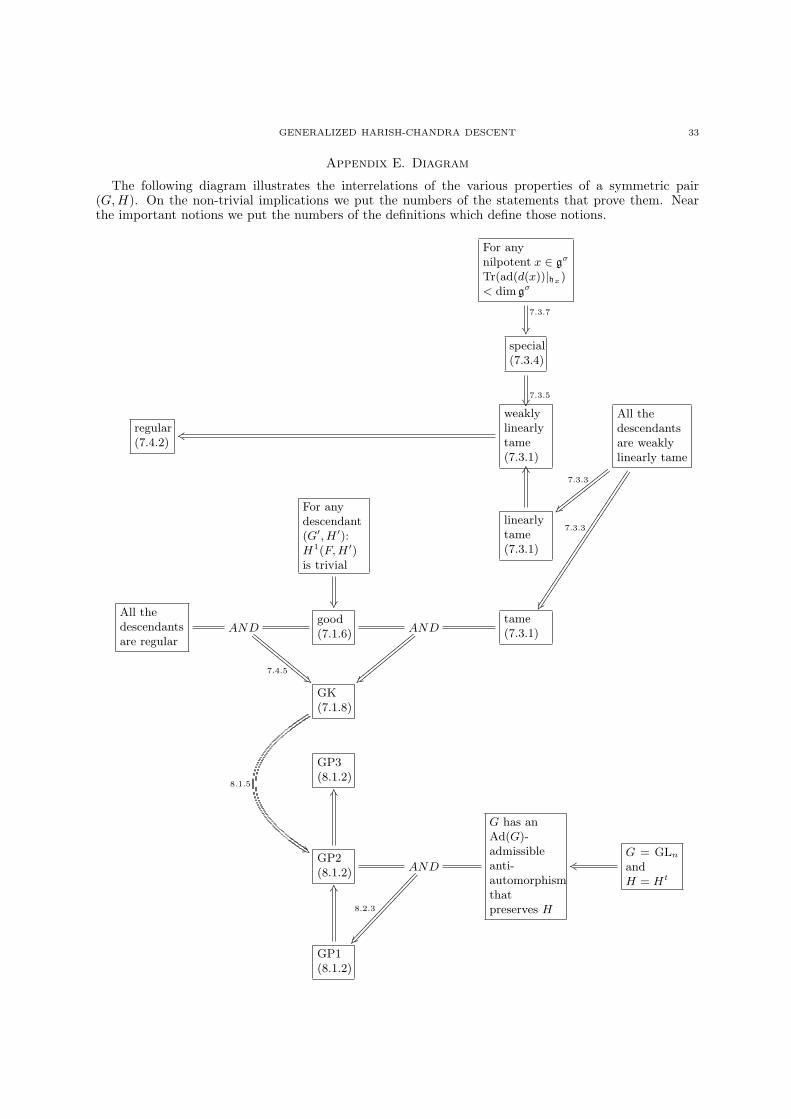
GENERALIZED HARISH-CHANDRA DESCENT 33
Appendix E. Diagram
The following diagram illustrates the interrelations of the various properties of a symmetric pair(G,H). On the non-trivial implications we put the numbers of the statements that prove them. Nearthe important notions we put the numbers of the definitions which define those notions.
For anynilpotent x ∈ gσ
Tr(ad(d(x))|hx)< dim gσ
7.3.7
special(7.3.4)
7.3.5
regular(7.4.2)
weaklylinearlytame(7.3.1)
ks
All thedescendantsare weaklylinearly tame
7.3.3
x xxxxxxxxxx
xxxxxxxxxx
7.3.3
For anydescendant(G′, H ′):H1(F, H ′)is trivial
linearlytame(7.3.1)
KS
All thedescendantsare regular
AND
7.4.5&
EEEEEEEEEEE
EEEEEEEEEEEgood(7.1.6) AND
x yyyyyyyyyyy
yyyyyyyyyyytame(7.3.1)
GK(7.1.8)
8.1.5
!)
GP3(8.1.2)
GP2(8.1.2)
KS
AND
8.2.3
|
G has anAd(G)-admissibleanti-automorphismthatpreserves H
G = GLn
andH = Ht
ks
GP1(8.1.2)
KS

34 AVRAHAM AIZENBUD AND DMITRY GOUREVITCH
References
[AG08a] A. Aizenbud, D. Gourevitch, Schwartz functions on Nash Manifolds, International Mathematics Research Notices,
Vol. 2008, n.5, Article ID rnm155, 37 pages. DOI: 10.1093/imrn/rnm155. See also arXiv:0704.2891 [math.AG].
[AG08b] Aizenbud, A.; Gourevitch, D.: De-Rham theorem and Shapiro lemma for Schwartz functions on Nash manifolds.To appear in the Israel Journal of Mathematics. See also arXiv:0802.3305v2 [math.AG].
[AG08c] Aizenbud, A.; Gourevitch, D.: Some regular symmetric pairs. To appear in Transactions of AMS. See also
arxiv:0805.2504[math.RT].[AGRS07] A. Aizenbud, D. Gourevitch, S. Rallis, G. Schiffmann, Multiplicity One Theorems, arXiv:0709.4215v1 [math.RT],
To appear in the Annals of Mathematics.
[AGS08] A. Aizenbud, D. Gourevitch, E. Sayag : (GLn+1(F ), GLn(F )) is a Gelfand pair for any local field F . CompositioMathematica, 144 , pp 1504-1524 (2008), doi:10.1112/S0010437X08003746. See also arXiv:0709.1273 [math.RT].
[AGS09] A. Aizenbud, D. Gourevitch, E. Sayag : (O(V ⊕ F ), O(V )) is a Gelfand pair for any quadratic space V
over a local field F , Mathematische Zeitschrift, 261 pp 239-244 (2009), DOI: 10.1007/s00209-008-0318-5. See alsoarXiv:0711.1471[math.RT].
[Aiz08] A. Aizenbud, A partial analog of integrability theorem for distributions on p-adic spaces and applications.
arXiv:0811.2768[math.RT].[AS08] A. Aizenbud, E. Sayag Invariant distributions on non-distinguished nilpotent orbits with application to the Gelfand
property of (GL(2n,R),Sp(2n,R)), arXiv:0810.1853 [math.RT].[Bar03] E.M. Baruch, A proof of Kirillov’s conjecture, Annals of Mathematics, 158, 207-252 (2003).
[BCR98] Bochnak, J.; Coste, M.; Roy, M-F.: Real Algebraic Geometry Berlin: Springer, 1998.
[Ber84] Joseph N. Bernstein, P -invariant distributions on GL(N) and the classification of unitary representations of GL(N)(non-Archimedean case), Lie group representations, II (College Park, Md., 1982/1983), Lecture Notes in Math., vol.
1041, Springer, Berlin, 1984, pp. 50–102. MR MR748505 (86b:22028)
[Brk71] D. Birkes, Orbits of linear algebraic groups, Ann. of Math. (2)93 (1971), 459-475.[BvD94] E. P. H. Bosman and G. Van Dijk, A New Class of Gelfand Pairs, Geometriae Dedicata 50, 261-282, 261 @ 1994
KluwerAcademic Publishers. Printed in the Netherlands (1994).
[BZ76] I. N. Bernsteın and A. V. Zelevinskiı, Representations of the group GL(n, F ), where F is a local non-Archimedeanfield, Uspehi Mat. Nauk 31 (1976), no. 3(189), 5–70. MR MR0425030 (54 #12988)
[Dre00] J.M.Drezet, Luna’s Slice Theorem And Applications, 23d Autumn School in Algebraic Geometry ”Algebraic group
actions and quotients” Wykno (Poland), (2000).[Fli91] Y.Z. Flicker: On distinguished representations, J. Reine Angew. Math. 418 (1991), 139-172.
[Gel76] S. Gelbart: Weil’s Representation and the Spectrum of the Metaplectic Group, Lecture Notes in Math., 530,Springer, Berlin-New York (1976).
[GK75] I. M. Gelfand and D. A. Kajdan, Representations of the group GL(n, K) where K is a local field, Lie groups and
their representations (Proc. Summer School, Bolyai Janos Math. Soc., Budapest, 1971), Halsted, New York, 1975,pp. 95–118. MR MR0404534 (53 #8334)
[Gro91] B. Gross, Some applications Gelfand pairs to number theory, Bull. Amer. Math. Soc. (N.S.) 24, no. 2, 277–301
(1991).[HC99] Harish-Chandra, Admissible invariant distributions on reductive p-adic groups, University Lecture Series, vol. 16,
American Mathematical Society, Providence, RI, 1999, Preface and notes by Stephen DeBacker and Paul J. Sally, Jr.
MR MR1702257 (2001b:22015)[Jac62] N. Jacobson, Lie Algebras, Interscience Tracts on Pure and Applied Mathematics, no. 10. Interscience Publishers,
New York (1962).
[JR96] Herve Jacquet and Stephen Rallis, Uniqueness of linear periods, Compositio Math. 102 (1996), no. 1, 65–123. MRMR1394521 (97k:22025)
[KR73] B. Kostant and S. Rallis, Orbits and representations associated with symmetric spaces, Amer. J. Math. 93 (1971),753-809.
[Lun73] D. Luna, Slices etales., Memoires de la Societe Mathematique de France, 33 (1973), p. 81-105
[Lun75] D. Luna, Sur certaines operations differentiables des groupes de Lie, Amer. J.Math. 97 (1975), 172-181.[Mum99] D. Mumford, The Red Book of Varieties and Schemes,second edition, Lecture Notes in Math., vol. 1358, Springer-
Verlag, New York, (1999).[Pra90] Dipendra Prasad, Trilinear forms for representations of GL(2) and local ε-factors, Compositio Math. 75 (1990),
no. 1, 1–46. MR MR1059954 (91i:22023)
[RS78] S. Rallis, G. Schiffmann, Automorphic Forms Constructed from the Weil Representation: Holomorphic Case, Amer-
ican Journal of Mathematics, Vol. 100, No. 5, pp. 1049-1122 (1978).[RS07] S. Rallis, G. Schiffmann, Multiplicity one Conjectures, arXiv:0705.2168v1 [math.RT].
[RR96] C. Rader and S. Rallis :Spherical Characters On p-Adic Symmetric Spaces, American Journal of Mathematics 118(1996), 91-178.
[Rud73] W. Rudin :Functional analysis New York : McGraw-Hill, 1973.
[Say08a] E. Sayag, (GL(2n,C),SP(2n,C)) is a Gelfand Pair. arXiv:0805.2625v1 [math.RT].[Say08b] E. Sayag, Regularity of invariant distributions on nice symmetric spaces and Gelfand property of symmetric pairs,
preprint.

GENERALIZED HARISH-CHANDRA DESCENT 35
[Ser64] J.P. Serre: Lie Algebras and Lie Groups Lecture Notes in Mathematics 1500, Springer-Verlag, New York, (1964).
[Sha74] J. Shalika, The multiplicity one theorem for GLn, Annals of Mathematics , 100, N.2, 171-193 (1974).
[Shi87] M. Shiota, Nash Manifolds, Lecture Notes in Mathematics 1269 (1987).[Tho84] E.G.F. Thomas, The theorem of Bochner-Schwartz-Godement for generalized Gelfand pairs, Functional Analysis:
Surveys and results III, Bierstedt, K.D., Fuchsteiner, B. (eds.), Elsevier Science Publishers B.V. (North Holland),(1984).
[vD86] G. van Dijk, On a class of generalized Gelfand pairs, Math. Z. 193, 581-593 (1986).
[vDP90] van Dijk, M. Poel, The irreducible unitary GLn−1(R)-spherical representations of SLn(R). Compositio Mathe-matica, 73 no. 1 (1990), p. 1-307.
[Wal88] N. Wallach, Real Reductive groups I, Pure and Applied Math. 132, Academic Press, Boston, MA (1988).
[Wal92] N. Wallach, Real Reductive groups II , Pure and Applied Math. 132-II, Academic Press, Boston, MA (1992).[Yak04] O. Yakimova, Gelfand pairs, PhD thesis submitted to Bonn university (2004). Availiable at
http : //bib.math.uni− bonn.de/pdf/BMS − 374.pdf
Avraham Aizenbud and Dmitry Gourevitch, Faculty of Mathematics and Computer Science, The Weizmann
Institute of Science POB 26, Rehovot 76100, ISRAEL.
E-mail address: [email protected]
E-mail address: [email protected]

![INTRODUCTION TO BANACH ALGEBRAS AND THE GELFAND-NAIMARK ...petrakis/INTRODUCTION TO BANACH ALGEBRAS.… · CONTENTS 1 A brief historical ... [Gelfand, Naimark 1943] Gelfand and Naimark3](https://img.pdfslide.us/doc/110x75/5aab82b47f8b9aa9488c1531/introduction-to-banach-algebras-and-the-gelfand-naimark-petrakisintroduction.jpg)