Embed Size (px)
Citation preview
Generalized Dedekind–Bernoulli Sums
A thesis presented to the faculty ofSan Francisco State University
In partial fulfilment ofThe Requirements for
The Degree
Master of ArtsIn
Mathematics
by
Anastasia Chavez
San Francisco, California
June 2010

Copyright byAnastasia Chavez
2010
CERTIFICATION OF APPROVAL
I certify that I have read Generalized Dedekind–Bernoulli Sums by Anas-
tasia Chavez and that in my opinion this work meets the criteria for
approving a thesis submitted in partial fulfillment of the requirements
for the degree: Master of Arts in Mathematics at San Francisco State
University.
Dr. Matthias BeckProfessor of Mathematics
Dr. Federico ArdilloProfessor of Mathematics
Dr. David EllisProfessor of Mathematics
Generalized Dedekind–Bernoulli Sums
Anastasia ChavezSan Francisco State University
2010
The finite arithmetic sum called a Dedekind sum appears in many areas of math-
ematics, such as topology, geometric combinatorics, algorithmic complexity, and
algebraic geometry. Dedekind sums exhibit many beautiful properties, the most fa-
mous being Dedekind’s reciprocity law. Since Dedekind, Apostol, Rademacher and
others have generalized Dedekind sums to involve Bernoulli polynomials. In 1995,
Hall, Wilson and Zagier introduced the 3-variable Dedekind-like sum and proved
a reciprocity relation. In this paper we introduce an n-variable generalization of
Hall, Wilson and Zagier’s sum called a multivariable Dedekind–Bernoulli sum and
prove a reciprocity law that generalizes the generic case of Hall, Wilson and Zagier’s
reciprocity theorem. Our proof uses a novel, combinatorial approach that simplifies
the proof of Hall, Wilson and Zagier’s reciprocity theorem and aids in proving the
general 4-variable extension of Hall, Wilson and Zagier’s reciprocity theorem.
I certify that the Abstract is a correct representation of the content of this thesis.
Chair, Thesis Committee Date

ACKNOWLEDGMENTS
I would like to thank my thesis advisor, collaborator and mentor, Dr.
Matthias Beck, for his support both academically and in life matters;
professor and mentor Dr. David Ellis, thank you for urging me to con-
tinue this mathematical path; many thanks to the talented and dedicated
professors and staff of the San Francisco State University Mathematics
Department for their support through the years; to my parents, thank
you for everything that was intentionally and unintentionally done, it
was and is exactly what I need to be me; to my husband and best friend,
Davi, your unconditional support and love helps me be the best version
of spirit that I can express, my endless gratitude to you resides in every
breath I take; and last, to the angels who bless my life in the most per-
fect ways, Ayla and Asha, thank you for your medicine and being the
profound teachers that you are.
v
TABLE OF CONTENTS
1 Introduction . . . . . . . . . . . . . . . . . . . . . . . . . . . . . . . . . . 1
2 More History, Definitions and Notations . . . . . . . . . . . . . . . . . . . 4
2.1 Bernoulli Polynomials and More . . . . . . . . . . . . . . . . . . . . . 4
2.2 Dedekind and Bernoulli meet . . . . . . . . . . . . . . . . . . . . . . 9
3 The Multivariate Dedekind–Bernoulli sum . . . . . . . . . . . . . . . . . . 12
4 A New Proof of Hall–Wilson–Zagier’s Reciprocity Theorem . . . . . . . . 42
5 The 4-variable reciprocity theorem . . . . . . . . . . . . . . . . . . . . . . 53
Bibliography . . . . . . . . . . . . . . . . . . . . . . . . . . . . . . . . . . . . 70
vi
Chapter 1
Introduction
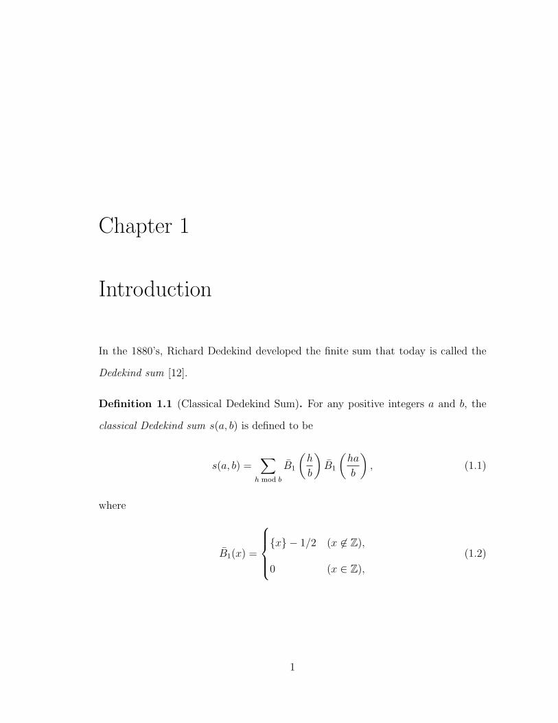
In the 1880’s, Richard Dedekind developed the finite sum that today is called the
Dedekind sum [12].
Definition 1.1 (Classical Dedekind Sum). For any positive integers a and b, the
classical Dedekind sum s(a, b) is defined to be
s(a, b) =∑
h mod b
B1
(h
b
)B1
(ha
b
), (1.1)
where
B1(x) =
x − 1/2 (x 6∈ Z),
0 (x ∈ Z),
(1.2)
1
2
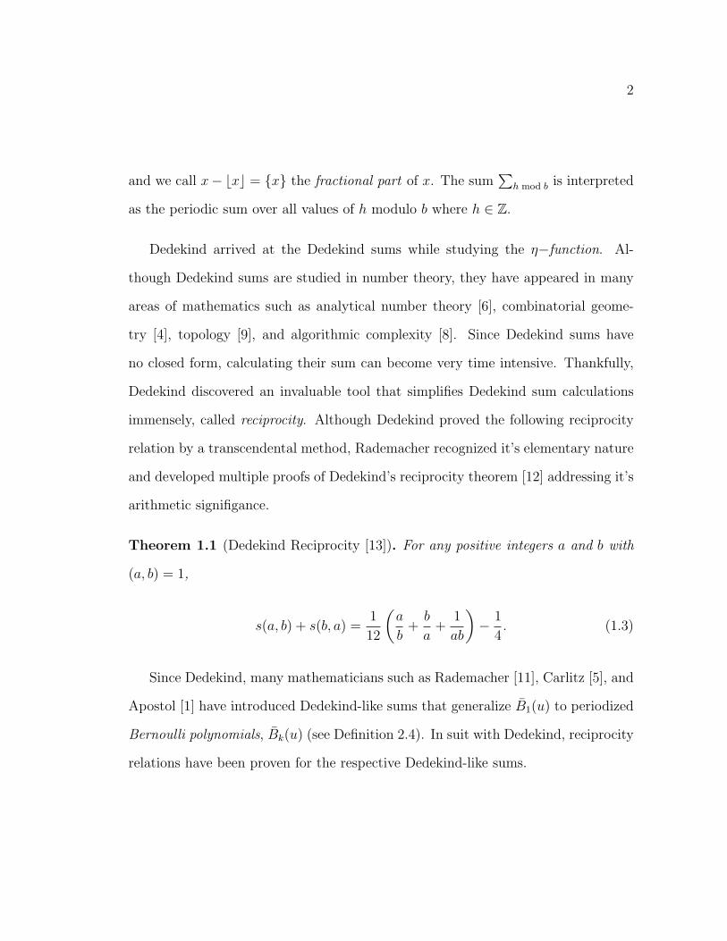
and we call x− bxc = x the fractional part of x. The sum∑
h mod b is interpreted
as the periodic sum over all values of h modulo b where h ∈ Z.
Dedekind arrived at the Dedekind sums while studying the η−function. Al-
though Dedekind sums are studied in number theory, they have appeared in many
areas of mathematics such as analytical number theory [6], combinatorial geome-
try [4], topology [9], and algorithmic complexity [8]. Since Dedekind sums have
no closed form, calculating their sum can become very time intensive. Thankfully,
Dedekind discovered an invaluable tool that simplifies Dedekind sum calculations
immensely, called reciprocity. Although Dedekind proved the following reciprocity
relation by a transcendental method, Rademacher recognized it’s elementary nature
and developed multiple proofs of Dedekind’s reciprocity theorem [12] addressing it’s
arithmetic signifigance.
Theorem 1.1 (Dedekind Reciprocity [13]). For any positive integers a and b with
(a, b) = 1,
s(a, b) + s(b, a) =1
12
(a
b+
b
a+
1
ab
)− 1
4. (1.3)
Since Dedekind, many mathematicians such as Rademacher [11], Carlitz [5], and
Apostol [1] have introduced Dedekind-like sums that generalize B1(u) to periodized
Bernoulli polynomials, Bk(u) (see Definition 2.4). In suit with Dedekind, reciprocity
relations have been proven for the respective Dedekind-like sums.
3
In 1995, Hall, Wilson and Zagier [7] introduced a generalization of Dedekind sums
(see Definition 2.4) that involve three variables and introduce shifts. They proved
a reciprocity theorem that is a wonderful example of how these relations express
the symmetry inherent in Dedekind-like sums and characterize their potential to be
evaluated so swiftly.
Most recent, Bayad and Raouj [3] have introduced a generalization of Hall, Wil-
son and Zagier’s sum and proved a reciprocity theorem that shows the non-generic
case of Hall, Wilson and Zagier’s reciprocity theorem is a special case.
In this paper we introduce a different generalization of Hall, Wilson and Zagier’s
sum called the multivariate Dedekind–Bernoulli sum (see Definition 3.1) and prove
our main result, a reciprocity theorem (see Theorem 3.1). Along with our main
result, we show that the generic case of Hall, Wilson and Zagier’s reciprocity theorem
follows from the proof of our reciprocity theorem and that one can say more about
the 4-variable version of Hall, Wilson and Zagier’s sum than is covered by the
reciprocity theorem given by Bayad and Raouj, as well as our own.
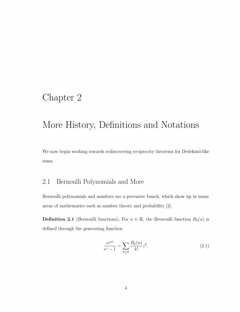
Chapter 2
More History, Definitions and Notations
We now begin working towards rediscovering reciprocity theorems for Dedekind-like
sums.
2.1 Bernoulli Polynomials and More
Bernoulli polynomials and numbers are a pervasive bunch, which show up in many
areas of mathematics such as number theory and probability [2].
Definition 2.1 (Bernoulli functions). For u ∈ R, the Bernoulli function Bk(u) is
defined through the generating function
zeuz
ez − 1=
∑k≥0
Bk(u)
k!zk. (2.1)
4
5
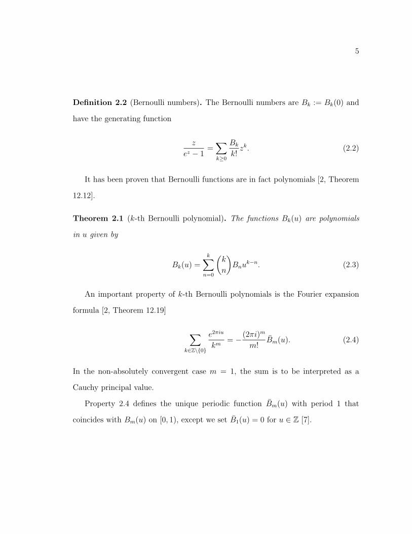
Definition 2.2 (Bernoulli numbers). The Bernoulli numbers are Bk := Bk(0) and
have the generating function
z
ez − 1=
∑k≥0
Bk
k!zk. (2.2)
It has been proven that Bernoulli functions are in fact polynomials [2, Theorem
12.12].
Theorem 2.1 (k-th Bernoulli polynomial). The functions Bk(u) are polynomials
in u given by
Bk(u) =k∑
n=0
(k
n
)Bnu
k−n. (2.3)
An important property of k-th Bernoulli polynomials is the Fourier expansion
formula [2, Theorem 12.19]
∑k∈Z\0
e2πiu
km= −(2πi)m
m!Bm(u). (2.4)
In the non-absolutely convergent case m = 1, the sum is to be interpreted as a
Cauchy principal value.
Property 2.4 defines the unique periodic function Bm(u) with period 1 that
coincides with Bm(u) on [0, 1), except we set B1(u) = 0 for u ∈ Z [7].
6
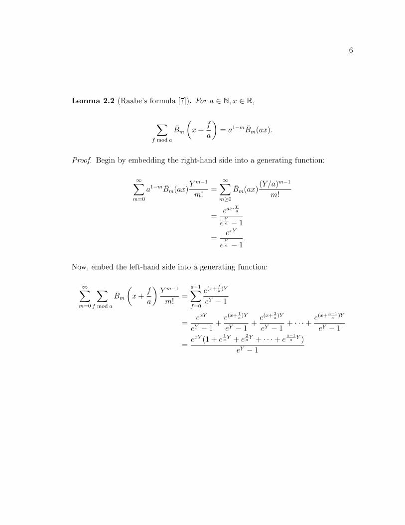
Lemma 2.2 (Raabe’s formula [7]). For a ∈ N, x ∈ R,
∑f mod a
Bm
(x +
f
a
)= a1−mBm(ax).
Proof. Begin by embedding the right-hand side into a generating function:
∞∑m=0
a1−mBm(ax)Y m−1
m!=
∞∑m≥0
Bm(ax)(Y/a)m−1
m!
=eax·Y
a
eYa − 1
=exY
eYa − 1
.
Now, embed the left-hand side into a generating function:
∞∑m=0
∑f mod a
Bm
(x +
f
a
)Y m−1
m!=
a−1∑f=0
e(x+ fa)Y
eY − 1
=exY
eY − 1+
e(x+ 1a)Y
eY − 1+
e(x+ 2a)Y
eY − 1+ · · ·+ e(x+a−1
a)Y
eY − 1
=exY (1 + e
1aY + e
2aY + · · ·+ e
a−1a
Y )
eY − 1
7
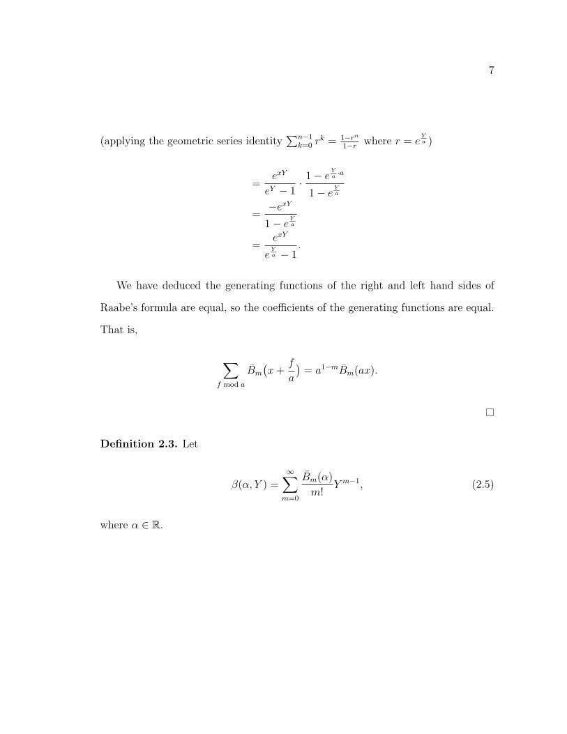
(applying the geometric series identity∑n−1
k=0 rk = 1−rn
1−rwhere r = e
Ya )
=exY
eY − 1· 1− e
Ya·a
1− eYa
=−exY
1− eYa
=exY
eYa − 1
.
We have deduced the generating functions of the right and left hand sides of
Raabe’s formula are equal, so the coefficients of the generating functions are equal.
That is,
∑f mod a
Bm
(x +
f
a
)= a1−mBm(ax).
Definition 2.3. Let
β(α, Y ) =∞∑
m=0
Bm(α)
m!Y m−1, (2.5)
where α ∈ R.
8
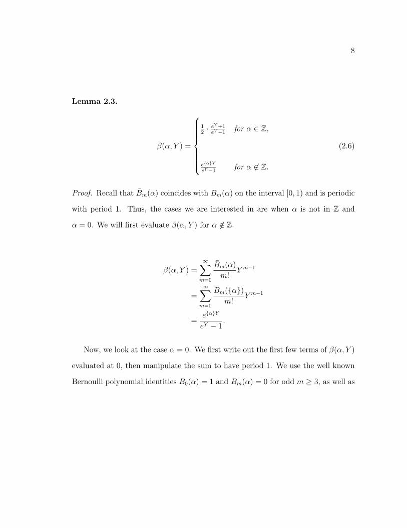
Lemma 2.3.
β(α, Y ) =
12· eY +1
eY −1for α ∈ Z,
eαY
eY −1for α 6∈ Z.
(2.6)
Proof. Recall that Bm(α) coincides with Bm(α) on the interval [0, 1) and is periodic
with period 1. Thus, the cases we are interested in are when α is not in Z and
α = 0. We will first evaluate β(α, Y ) for α 6∈ Z.
β(α, Y ) =∞∑
m=0
Bm(α)
m!Y m−1
=∞∑
m=0
Bm(α)m!
Y m−1
=eαY
eY − 1.
Now, we look at the case α = 0. We first write out the first few terms of β(α, Y )
evaluated at 0, then manipulate the sum to have period 1. We use the well known
Bernoulli polynomial identities B0(α) = 1 and Bm(α) = 0 for odd m ≥ 3, as well as
9
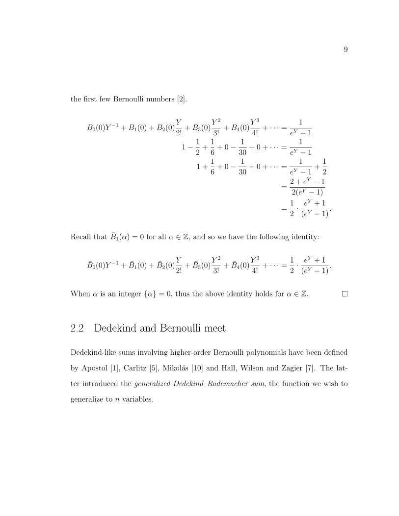
the first few Bernoulli numbers [2].
B0(0)Y −1 + B1(0) + B2(0)Y
2!+ B3(0)
Y 2
3!+ B4(0)
Y 3
4!+ · · · = 1
eY − 1
1− 1
2+
1
6+ 0− 1
30+ 0 + · · · = 1
eY − 1
1 +1
6+ 0− 1
30+ 0 + · · · = 1
eY − 1+
1
2
=2 + eY − 1
2(eY − 1)
=1
2· eY + 1
(eY − 1).
Recall that B1(α) = 0 for all α ∈ Z, and so we have the following identity:
B0(0)Y −1 + B1(0) + B2(0)Y
2!+ B3(0)
Y 2
3!+ B4(0)
Y 3
4!+ · · · = 1
2· eY + 1
(eY − 1).
When α is an integer α = 0, thus the above identity holds for α ∈ Z.
2.2 Dedekind and Bernoulli meet
Dedekind-like sums involving higher-order Bernoulli polynomials have been defined
by Apostol [1], Carlitz [5], Mikolas [10] and Hall, Wilson and Zagier [7]. The lat-
ter introduced the generalized Dedekind–Rademacher sum, the function we wish to
generalize to n variables.
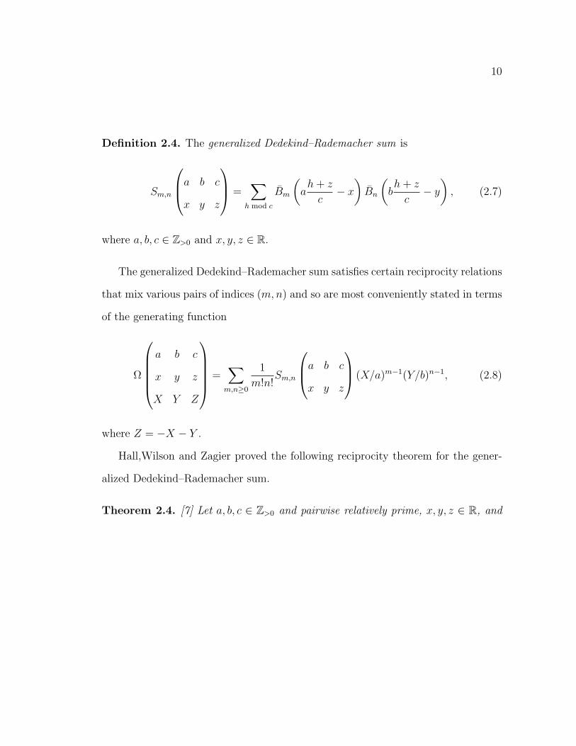
10
Definition 2.4. The generalized Dedekind–Rademacher sum is
Sm,n
a b c
x y z
=∑
h mod c
Bm
(ah + z
c− x
)Bn
(bh + z
c− y
), (2.7)
where a, b, c ∈ Z>0 and x, y, z ∈ R.
The generalized Dedekind–Rademacher sum satisfies certain reciprocity relations
that mix various pairs of indices (m, n) and so are most conveniently stated in terms
of the generating function
Ω
a b c
x y z
X Y Z
=∑
m,n≥0
1
m!n!Sm,n
a b c
x y z
(X/a)m−1(Y/b)n−1, (2.8)
where Z = −X − Y .
Hall,Wilson and Zagier proved the following reciprocity theorem for the gener-
alized Dedekind–Rademacher sum.
Theorem 2.4. [7] Let a, b, c ∈ Z>0 and pairwise relatively prime, x, y, z ∈ R, and
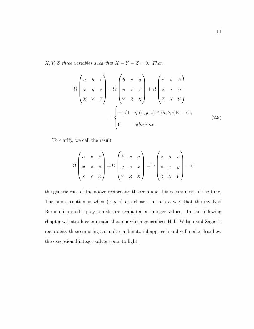
11
X, Y, Z three variables such that X + Y + Z = 0. Then
Ω
a b c
x y z
X Y Z
+ Ω
b c a
y z x
Y Z X
+ Ω
c a b
z x y
Z X Y
=
−1/4 if (x, y, z) ∈ (a, b, c)R + Z3,
0 otherwise.
(2.9)
To clarify, we call the result
Ω
a b c
x y z
X Y Z
+ Ω
b c a
y z x
Y Z X
+ Ω
c a b
z x y
Z X Y
= 0
the generic case of the above reciprocity theorem and this occurs most of the time.
The one exception is when (x, y, z) are chosen in such a way that the involved
Bernoulli periodic polynomials are evaluated at integer values. In the following
chapter we introduce our main theorem which generalizes Hall, Wilson and Zagier’s
reciprocity theorem using a simple combinatorial approach and will make clear how
the exceptional integer values come to light.
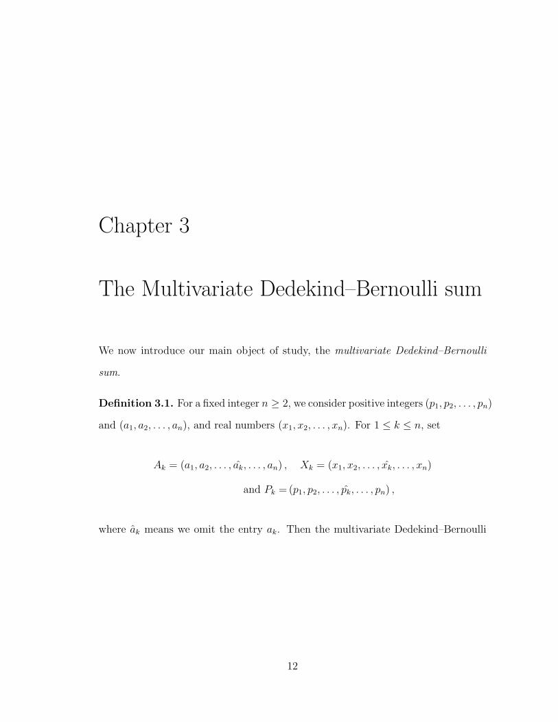
Chapter 3
The Multivariate Dedekind–Bernoulli sum
We now introduce our main object of study, the multivariate Dedekind–Bernoulli
sum.
Definition 3.1. For a fixed integer n ≥ 2, we consider positive integers (p1, p2, . . . , pn)
and (a1, a2, . . . , an), and real numbers (x1, x2, . . . , xn). For 1 ≤ k ≤ n, set
Ak = (a1, a2, . . . , ak, . . . , an) , Xk = (x1, x2, . . . , xk, . . . , xn)
and Pk = (p1, p2, . . . , pk, . . . , pn) ,
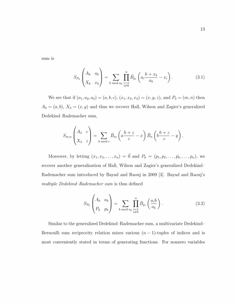
where ak means we omit the entry ak. Then the multivariate Dedekind–Bernoulli
12
13
sum is
SPk
Ak ak
Xk xk
=∑
h mod ak
n∏i=1i6=k
Bpi
(ai
h + xk
ak
− xi
). (3.1)
We see that if (a1, a2, a3) = (a, b, c), (x1, x2, x3) = (x, y, z), and P3 = (m, n) then
A3 = (a, b), X3 = (x, y) and thus we recover Hall, Wilson and Zagier’s generalized
Dedekind–Rademacher sum,
Sm,n
A3 c
X3 z
=∑
h mod c
Bm
(ah + z
c− x
)Bn
(bh + z
c− y
).
Moreover, by letting (x1, x2, . . . , xn) = ~0 and Pk = (p1, p2, . . . , pk, . . . , pn), we
recover another generalization of Hall, Wilson and Zagier’s generalized Dedekind–
Rademacher sum introduced by Bayad and Raouj in 2009 [3]. Bayad and Raouj’s
multiple Dedekind–Rademacher sum is thus defined
SPk
Ak ak
Pk pk
=∑
h mod ak
n∏i=1i6=k
Bpi
(aih
ak
). (3.2)
Similar to the generalized Dedekind–Rademacher sum, a multivariate Dedekind–
Bernoulli sum reciprocity relation mixes various (n− 1)-tuples of indices and is
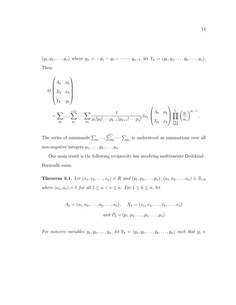
most conveniently stated in terms of generating functions. For nonzero variables
14
(y1, y2, . . . , yn) where yn = −y1 − y2 − · · · − yn−1, let Yk = (y1, y2, . . . , yk, . . . , yn).
Then
Ω
Ak ak
Xk xk
Yk yk
=
∑p1
. . .∑pk
· · ·∑pn
1
p1!p2! · · · pk−1!pk+1! · · · pn!SPk
Ak ak
Xk xk
n∏i=1i6=k
(yi
ai
)pi−1
.
The series of summands∑
p1. . .
∑pk· · ·
∑pn
is understood as summations over all
non-negative integers p1, . . . , pk, . . . , pn.
Our main result is the following reciprocity law involving multivariate Dedekind–
Bernoulli sums.
Theorem 3.1. Let (x1, x2, . . . , xn) ∈ R and (p1, p2, . . . , pn) , (a1, a2, . . . , an) ∈ Z>0
where (au, av) = 1 for all 1 ≤ u < v ≤ n. For 1 ≤ k ≤ n, let
Ak = (a1, a2, . . . , ak, . . . , an) , Xk = (x1, x2, . . . , xk, . . . , xn)
and Pk = (p1, p2, . . . , pk, . . . , pn) .
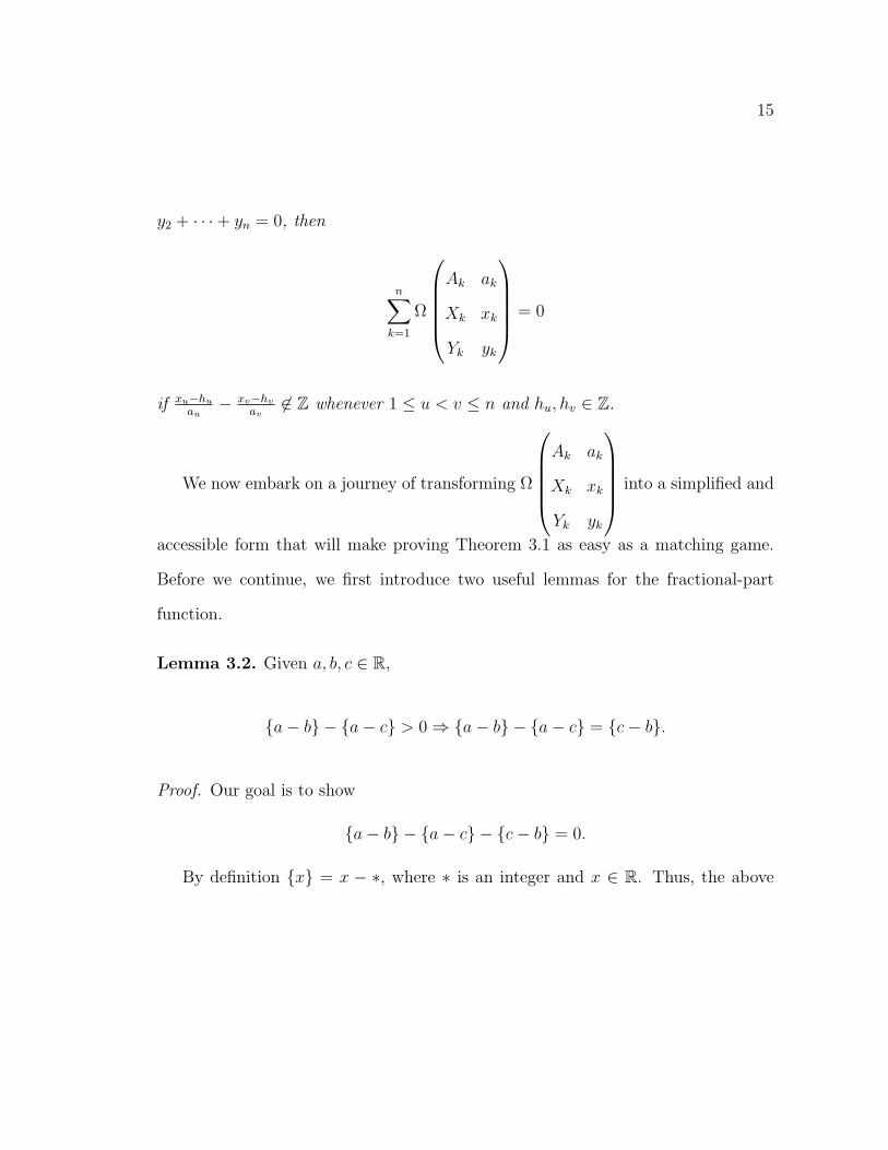
For nonzero variables y1, y2, . . . , yn, let Yk = (y1, y2, . . . , yk, . . . , yn) such that y1 +
15
y2 + · · ·+ yn = 0, then
n∑k=1
Ω
Ak ak
Xk xk
Yk yk
= 0
if xu−hu
au− xv−hv
av6∈ Z whenever 1 ≤ u < v ≤ n and hu, hv ∈ Z.
We now embark on a journey of transforming Ω
Ak ak
Xk xk
Yk yk
into a simplified and
accessible form that will make proving Theorem 3.1 as easy as a matching game.
Before we continue, we first introduce two useful lemmas for the fractional-part
function.
Lemma 3.2. Given a, b, c ∈ R,
a− b − a− c > 0 ⇒ a− b − a− c = c− b.
Proof. Our goal is to show
a− b − a− c − c− b = 0.
By definition x = x − ∗, where ∗ is an integer and x ∈ R. Thus, the above
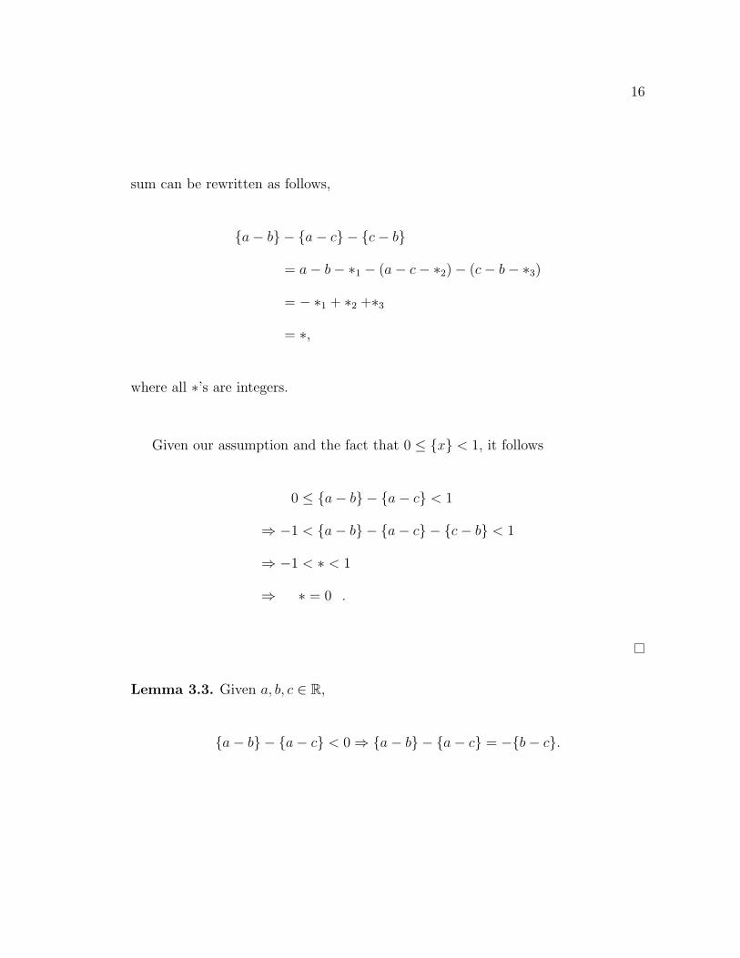
16
sum can be rewritten as follows,
a− b − a− c − c− b
= a− b− ∗1 − (a− c− ∗2)− (c− b− ∗3)
= − ∗1 + ∗2 +∗3
= ∗,
where all ∗’s are integers.
Given our assumption and the fact that 0 ≤ x < 1, it follows
0 ≤ a− b − a− c < 1
⇒ −1 < a− b − a− c − c− b < 1
⇒ −1 < ∗ < 1
⇒ ∗ = 0 .
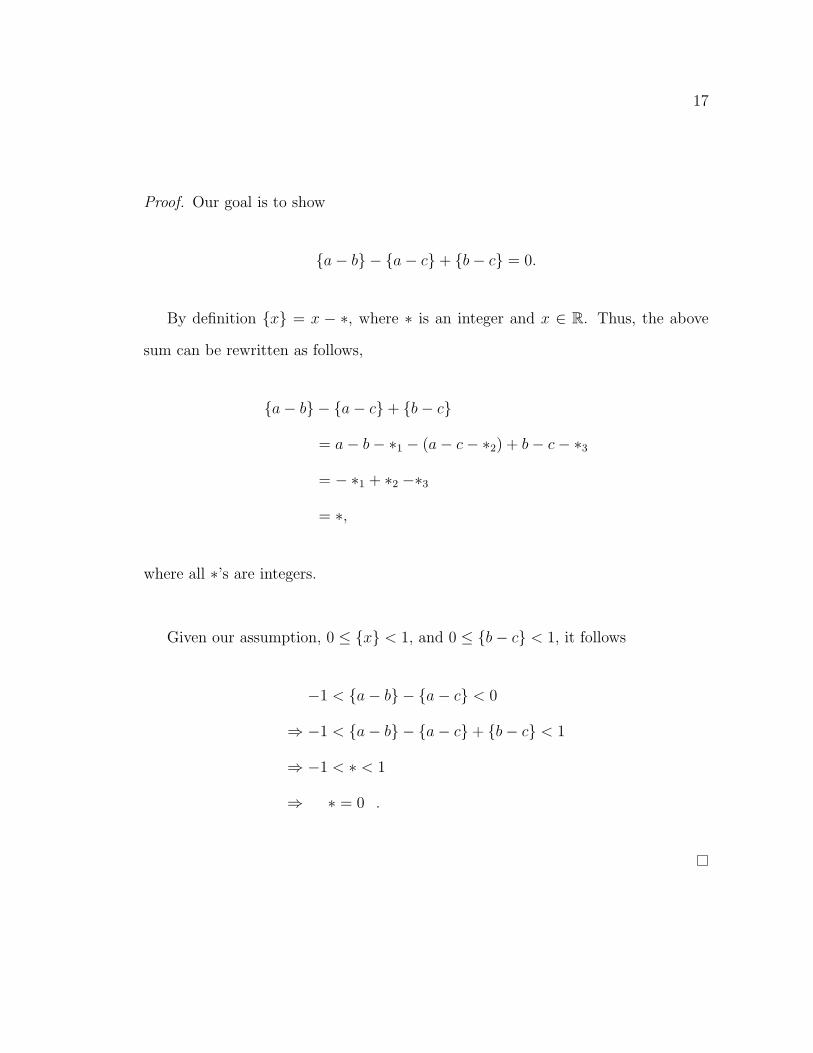
Lemma 3.3. Given a, b, c ∈ R,
a− b − a− c < 0 ⇒ a− b − a− c = −b− c.
17
Proof. Our goal is to show
a− b − a− c+ b− c = 0.
By definition x = x − ∗, where ∗ is an integer and x ∈ R. Thus, the above
sum can be rewritten as follows,
a− b − a− c+ b− c
= a− b− ∗1 − (a− c− ∗2) + b− c− ∗3
= − ∗1 + ∗2 −∗3
= ∗,
where all ∗’s are integers.
Given our assumption, 0 ≤ x < 1, and 0 ≤ b− c < 1, it follows
−1 < a− b − a− c < 0
⇒ −1 < a− b − a− c+ b− c < 1
⇒ −1 < ∗ < 1
⇒ ∗ = 0 .
18
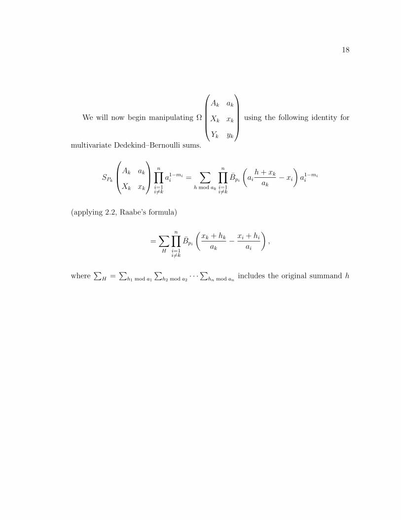
We will now begin manipulating Ω
Ak ak
Xk xk
Yk yk
using the following identity for
multivariate Dedekind–Bernoulli sums.
SPk
Ak ak
Xk xk
n∏i=1i6=k
a1−mii =
∑h mod ak
n∏i=1i6=k
Bpi
(ai
h + xk
ak
− xi
)a1−mi
i
(applying 2.2, Raabe’s formula)
=∑H
n∏i=1i6=k
Bpi
(xk + hk
ak
− xi + hi
ai
),
where∑
H =∑
h1 mod a1
∑h2 mod a2
· · ·∑
hn mod anincludes the original summand h
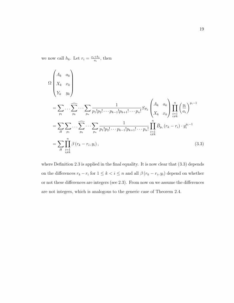
19
we now call hk. Let ri = xi+hi
ai, then
Ω
Ak ak
Xk xk
Yk yk
=
∑p1
. . .∑pk
· · ·∑pn
1
p1!p2! · · · pk−1!pk+1! · · · pn!SPk
Ak ak
Xk xk
n∏i=1i6=k
(yi
ai
)pi−1
=∑H
∑p1
. . .∑pk
· · ·∑pn
1
p1!p2! · · · pk−1!pk+1! · · · pn!
n∏i=1i6=k
Bpi(rk − ri) · ypi−1
i
=∑H
n∏i=1i6=k
β (rk − ri, yi) , (3.3)
where Definition 2.3 is applied in the final equality. It is now clear that (3.3) depends
on the differences rk− ri for 1 ≤ k < i ≤ n and all β (rk − ri, yi) depend on whether
or not these differences are integers (see 2.3). From now on we assume the differences
are not integers, which is analogous to the generic case of Theorem 2.4.
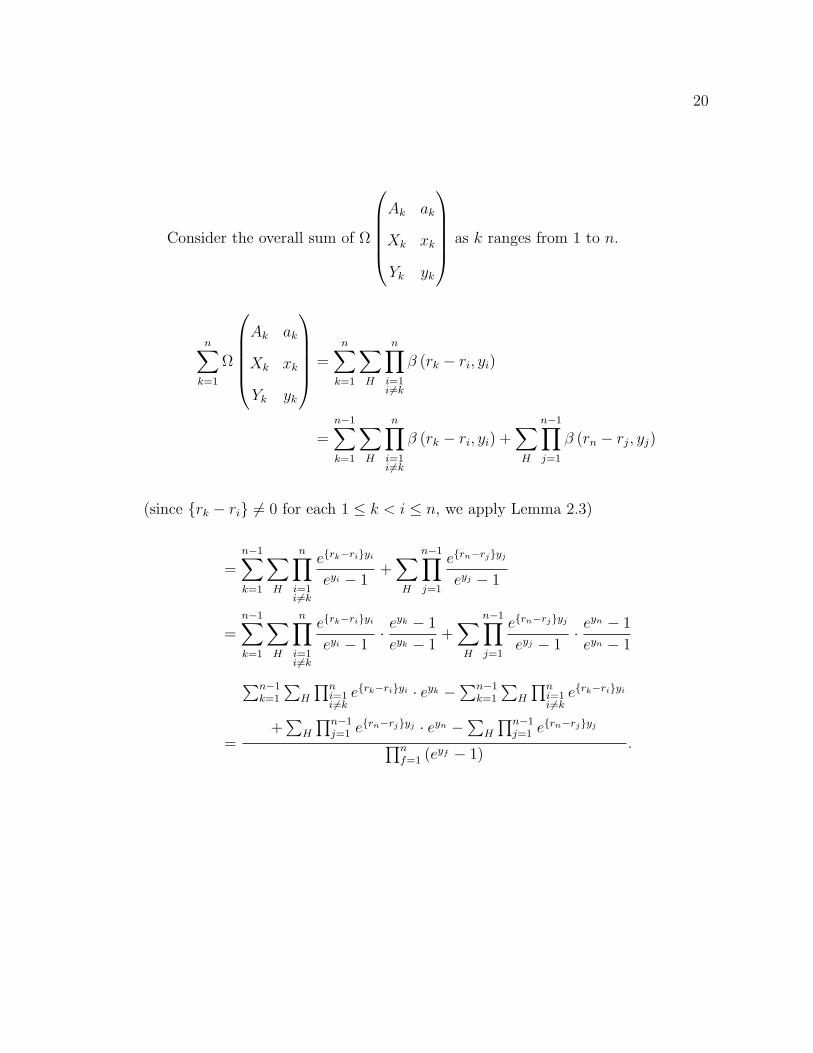
20
Consider the overall sum of Ω
Ak ak
Xk xk
Yk yk
as k ranges from 1 to n.
n∑k=1
Ω
Ak ak
Xk xk
Yk yk
=n∑
k=1
∑H
n∏i=1i6=k
β (rk − ri, yi)
=n−1∑k=1
∑H
n∏i=1i6=k
β (rk − ri, yi) +∑H
n−1∏j=1
β (rn − rj, yj)
(since rk − ri 6= 0 for each 1 ≤ k < i ≤ n, we apply Lemma 2.3)
=n−1∑k=1
∑H
n∏i=1i6=k
erk−riyi
eyi − 1+
∑H
n−1∏j=1
ern−rjyj
eyj − 1
=n−1∑k=1
∑H
n∏i=1i6=k
erk−riyi
eyi − 1· eyk − 1
eyk − 1+
∑H
n−1∏j=1
ern−rjyj
eyj − 1· eyn − 1
eyn − 1
=
∑n−1k=1
∑H
∏ni=1i6=k
erk−riyi · eyk −∑n−1
k=1
∑H
∏ni=1i6=k
erk−riyi
+∑
H
∏n−1j=1 ern−rjyj · eyn −
∑H
∏n−1j=1 ern−rjyj∏n
f=1 (eyf − 1).
21
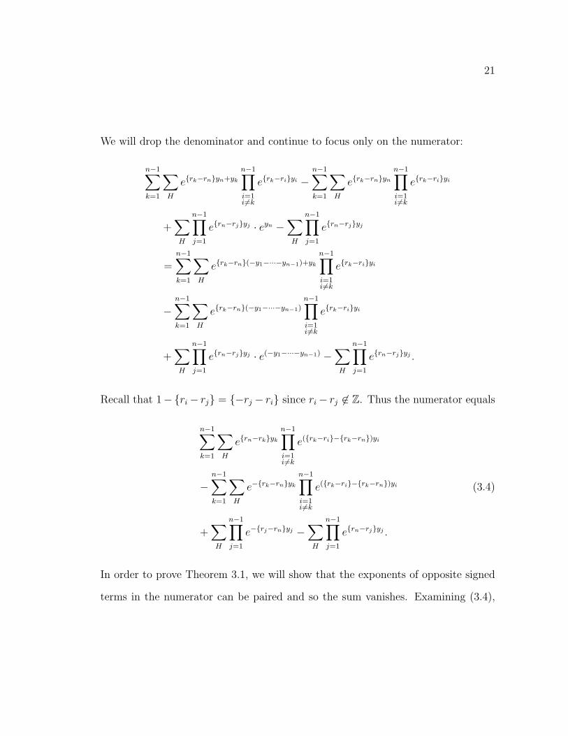
We will drop the denominator and continue to focus only on the numerator:
n−1∑k=1
∑H
erk−rnyn+yk
n−1∏i=1i6=k
erk−riyi −n−1∑k=1
∑H
erk−rnyn
n−1∏i=1i6=k
erk−riyi
+∑H
n−1∏j=1
ern−rjyj · eyn −∑H
n−1∏j=1
ern−rjyj
=n−1∑k=1
∑H
erk−rn(−y1−···−yn−1)+yk
n−1∏i=1i6=k
erk−riyi
−n−1∑k=1
∑H
erk−rn(−y1−···−yn−1)
n−1∏i=1i6=k
erk−riyi
+∑H
n−1∏j=1
ern−rjyj · e(−y1−···−yn−1) −∑H
n−1∏j=1
ern−rjyj .
Recall that 1−ri − rj = −rj − ri since ri − rj 6∈ Z. Thus the numerator equals
n−1∑k=1
∑H
ern−rkyk
n−1∏i=1i6=k
e(rk−ri−rk−rn)yi
−n−1∑k=1
∑H
e−rk−rnyk
n−1∏i=1i6=k
e(rk−ri−rk−rn)yi (3.4)
+∑H
n−1∏j=1
e−rj−rnyj −∑H
n−1∏j=1
ern−rjyj .
In order to prove Theorem 3.1, we will show that the exponents of opposite signed
terms in the numerator can be paired and so the sum vanishes. Examining (3.4),
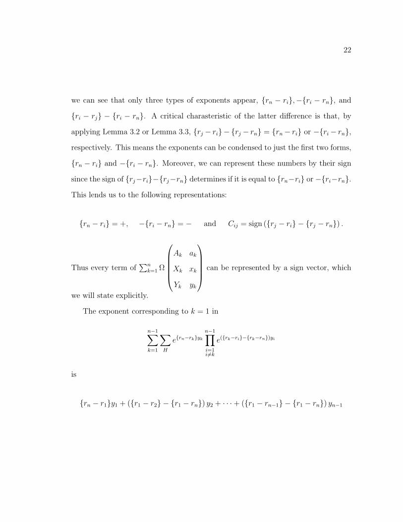
22
we can see that only three types of exponents appear, rn − ri,−ri − rn, and
ri − rj − ri − rn. A critical charasteristic of the latter difference is that, by
applying Lemma 3.2 or Lemma 3.3, rj − ri− rj − rn = rn − ri or −ri − rn,
respectively. This means the exponents can be condensed to just the first two forms,
rn − ri and −ri − rn. Moreover, we can represent these numbers by their sign
since the sign of rj−ri−rj−rn determines if it is equal to rn−ri or −ri−rn.
This lends us to the following representations:
rn − ri = +, −ri − rn = − and Cij = sign (rj − ri − rj − rn) .
Thus every term of∑n
k=1 Ω
Ak ak
Xk xk
Yk yk
can be represented by a sign vector, which
we will state explicitly.
The exponent corresponding to k = 1 in
n−1∑k=1
∑H
ern−rkyk
n−1∏i=1i6=k
e(rk−ri−rk−rn)yi
is
rn − r1y1 + (r1 − r2 − r1 − rn) y2 + · · ·+ (r1 − rn−1 − r1 − rn) yn−1
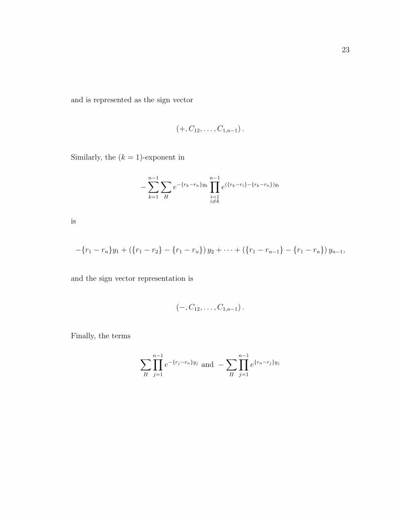
23
and is represented as the sign vector
(+, C12, . . . , C1,n−1) .
Similarly, the (k = 1)-exponent in
−n−1∑k=1
∑H
e−rk−rnyk
n−1∏i=1i6=k
e(rk−ri−rk−rn)yi
is
−r1 − rny1 + (r1 − r2 − r1 − rn) y2 + · · ·+ (r1 − rn−1 − r1 − rn) yn−1,
and the sign vector representation is
(−, C12, . . . , C1,n−1) .
Finally, the terms
∑H
n−1∏j=1
e−rj−rnyj and −∑H
n−1∏j=1
ern−rjyj
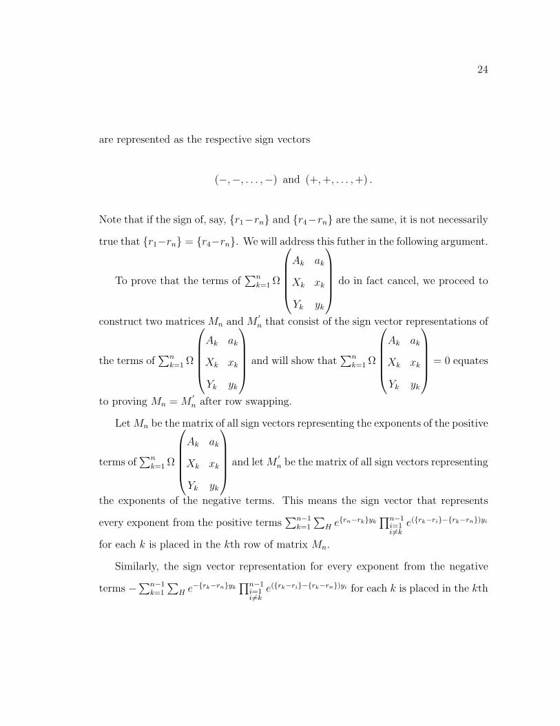
24
are represented as the respective sign vectors
(−,−, . . . ,−) and (+, +, . . . , +) .
Note that if the sign of, say, r1−rn and r4−rn are the same, it is not necessarily
true that r1−rn = r4−rn. We will address this futher in the following argument.
To prove that the terms of∑n
k=1 Ω
Ak ak
Xk xk
Yk yk
do in fact cancel, we proceed to
construct two matrices Mn and M′n that consist of the sign vector representations of
the terms of∑n
k=1 Ω
Ak ak
Xk xk
Yk yk
and will show that∑n
k=1 Ω
Ak ak
Xk xk
Yk yk
= 0 equates
to proving Mn = M′n after row swapping.
Let Mn be the matrix of all sign vectors representing the exponents of the positive
terms of∑n
k=1 Ω
Ak ak
Xk xk
Yk yk
and let M′n be the matrix of all sign vectors representing
the exponents of the negative terms. This means the sign vector that represents
every exponent from the positive terms∑n−1
k=1
∑H ern−rkyk
∏n−1i=1i6=k
e(rk−ri−rk−rn)yi
for each k is placed in the kth row of matrix Mn.
Similarly, the sign vector representation for every exponent from the negative
terms −∑n−1
k=1
∑H e−rk−rnyk
∏n−1i=1i6=k
e(rk−ri−rk−rn)yi for each k is placed in the kth
25
row of the matrix M′n.
Finally, place the sign vector representing∑
H
∏n−1j=1 e−rj−rnyj in the last row
of Mn and the sign vector representing −∑
H
∏n−1j=1 ern−rjyj in the last row of M
′n.
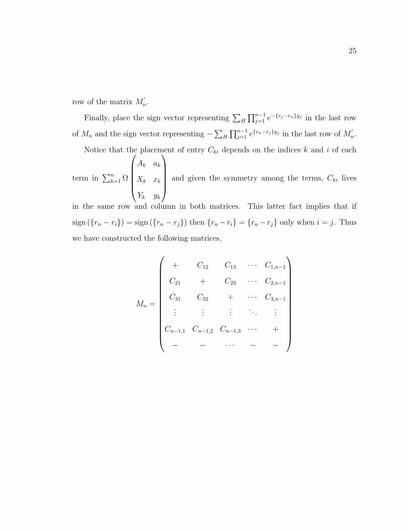
Notice that the placement of entry Cki depends on the indices k and i of each
term in∑n
k=1 Ω
Ak ak
Xk xk
Yk yk
and given the symmetry among the terms, Cki lives
in the same row and column in both matrices. This latter fact implies that if
sign (rn − ri) = sign (rn − rj) then rn− ri = rn− rj only when i = j. Thus
we have constructed the following matrices,
Mn =
+ C12 C13 · · · C1,n−1
C21 + C23 · · · C2,n−1
C31 C32 + · · · C3,n−1
......
.... . .
...
Cn−1,1 Cn−1,2 Cn−1,3 · · · +
− − · · · − −

26
and
M′
n =
− C12 C13 · · · C1,n−1
C21 − C23 · · · C2,n−1
C31 C32 − · · · C3,n−1
......
.... . .
...
Cn−1,1 Cn−1,2 Cn−1,3 · · · −
+ + · · · + +
.
Last, we will show that Mn = M′n after row swapping implies
∑nk=1 Ω
Ak ak
Xk xk
Yk yk
vanishes. Assume Mn = M
′n up to row swapping. Then for each sign row vector
(Cs1, . . . , Cs,s−1, +, Cs,s+1, . . . , Cs,n−1) ∈ Mn
there exists
(Ct1, . . . , Ct,t−1,−, Ct,t+1, . . . , Ct,n−1) ∈ M′
n
such that
(Cs1, . . . , Cs,s−1, +, Cs,s+1, . . . , Cs,n−1) = (Ct1, . . . , Ct,t−1,−, Ct,t+1, . . . , Ct,n−1) .
27
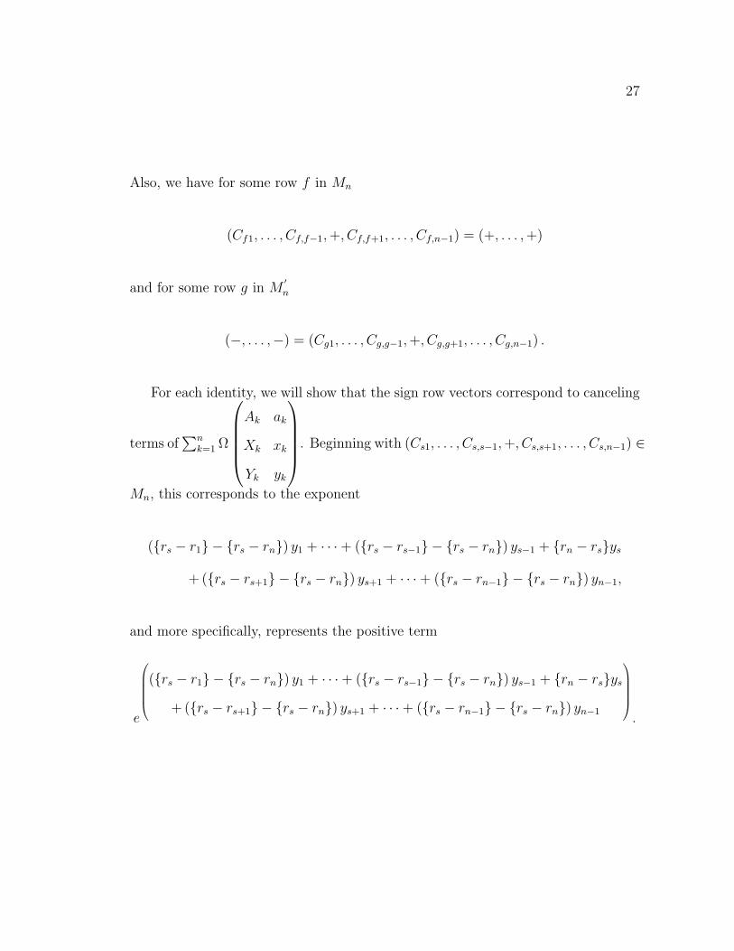
Also, we have for some row f in Mn
(Cf1, . . . , Cf,f−1, +, Cf,f+1, . . . , Cf,n−1) = (+, . . . , +)
and for some row g in M′n
(−, . . . ,−) = (Cg1, . . . , Cg,g−1, +, Cg,g+1, . . . , Cg,n−1) .
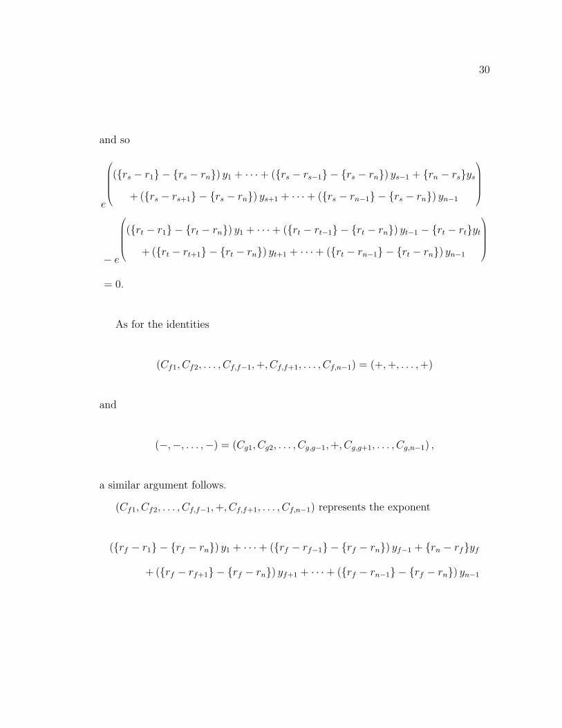
For each identity, we will show that the sign row vectors correspond to canceling
terms of∑n
k=1 Ω
Ak ak
Xk xk
Yk yk
. Beginning with (Cs1, . . . , Cs,s−1, +, Cs,s+1, . . . , Cs,n−1) ∈
Mn, this corresponds to the exponent
(rs − r1 − rs − rn) y1 + · · ·+ (rs − rs−1 − rs − rn) ys−1 + rn − rsys
+ (rs − rs+1 − rs − rn) ys+1 + · · ·+ (rs − rn−1 − rs − rn) yn−1,
and more specifically, represents the positive term
e
0BBBB@(rs − r1 − rs − rn) y1 + · · ·+ (rs − rs−1 − rs − rn) ys−1 + rn − rsys
+ (rs − rs+1 − rs − rn) ys+1 + · · ·+ (rs − rn−1 − rs − rn) yn−1
1CCCCA.
28
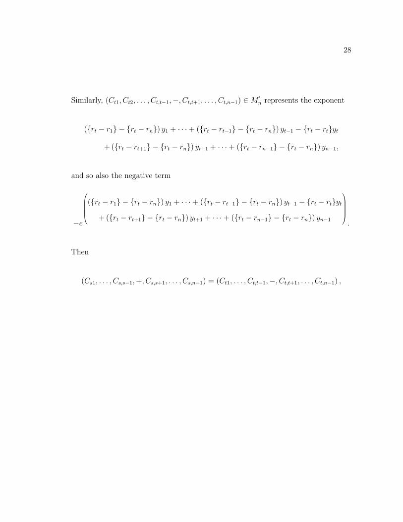
Similarly, (Ct1, Ct2, . . . , Ct,t−1,−, Ct,t+1, . . . , Ct,n−1) ∈ M′n represents the exponent
(rt − r1 − rt − rn) y1 + · · ·+ (rt − rt−1 − rt − rn) yt−1 − rt − rtyt
+ (rt − rt+1 − rt − rn) yt+1 + · · ·+ (rt − rn−1 − rt − rn) yn−1,
and so also the negative term
−e
0BBBB@(rt − r1 − rt − rn) y1 + · · ·+ (rt − rt−1 − rt − rn) yt−1 − rt − rtyt
+ (rt − rt+1 − rt − rn) yt+1 + · · ·+ (rt − rn−1 − rt − rn) yn−1
1CCCCA.
Then
(Cs1, . . . , Cs,s−1, +, Cs,s+1, . . . , Cs,n−1) = (Ct1, . . . , Ct,t−1,−, Ct,t+1, . . . , Ct,n−1) ,
29
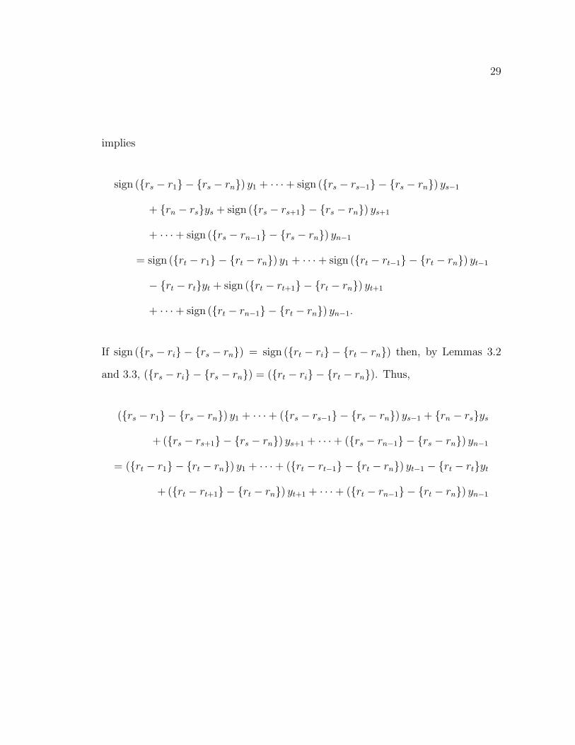
implies
sign (rs − r1 − rs − rn) y1 + · · ·+ sign (rs − rs−1 − rs − rn) ys−1
+ rn − rsys + sign (rs − rs+1 − rs − rn) ys+1
+ · · ·+ sign (rs − rn−1 − rs − rn) yn−1
= sign (rt − r1 − rt − rn) y1 + · · ·+ sign (rt − rt−1 − rt − rn) yt−1
− rt − rtyt + sign (rt − rt+1 − rt − rn) yt+1
+ · · ·+ sign (rt − rn−1 − rt − rn) yn−1.
If sign (rs − ri − rs − rn) = sign (rt − ri − rt − rn) then, by Lemmas 3.2
and 3.3, (rs − ri − rs − rn) = (rt − ri − rt − rn). Thus,
(rs − r1 − rs − rn) y1 + · · ·+ (rs − rs−1 − rs − rn) ys−1 + rn − rsys
+ (rs − rs+1 − rs − rn) ys+1 + · · ·+ (rs − rn−1 − rs − rn) yn−1
= (rt − r1 − rt − rn) y1 + · · ·+ (rt − rt−1 − rt − rn) yt−1 − rt − rtyt
+ (rt − rt+1 − rt − rn) yt+1 + · · ·+ (rt − rn−1 − rt − rn) yn−1
30
and so
e
0BBBB@(rs − r1 − rs − rn) y1 + · · ·+ (rs − rs−1 − rs − rn) ys−1 + rn − rsys
+ (rs − rs+1 − rs − rn) ys+1 + · · ·+ (rs − rn−1 − rs − rn) yn−1
1CCCCA
− e
0BBBB@(rt − r1 − rt − rn) y1 + · · ·+ (rt − rt−1 − rt − rn) yt−1 − rt − rtyt
+ (rt − rt+1 − rt − rn) yt+1 + · · ·+ (rt − rn−1 − rt − rn) yn−1
1CCCCA
= 0.
As for the identities
(Cf1, Cf2, . . . , Cf,f−1, +, Cf,f+1, . . . , Cf,n−1) = (+, +, . . . , +)
and
(−,−, . . . ,−) = (Cg1, Cg2, . . . , Cg,g−1, +, Cg,g+1, . . . , Cg,n−1) ,
a similar argument follows.
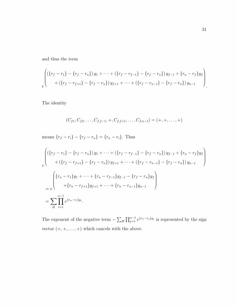
(Cf1, Cf2, . . . , Cf,f−1, +, Cf,f+1, . . . , Cf,n−1) represents the exponent
(rf − r1 − rf − rn) y1 + · · ·+ (rf − rf−1 − rf − rn) yf−1 + rn − rfyf
+ (rf − rf+1 − rf − rn) yf+1 + · · ·+ (rf − rn−1 − rf − rn) yn−1
31
and thus the term
e
0BBBB@(rf − r1 − rf − rn) y1 + · · ·+ (rf − rf−1 − rf − rn) yf−1 + rn − rfyf
+ (rf − rf+1 − rf − rn) yf+1 + · · ·+ (rf − rn−1 − rf − rn) yn−1
1CCCCA.
The identity
(Cf1, Cf2, . . . , Cf,f−1, +, Cf,f+1, . . . , Cf,n−1) = (+, +, . . . , +)
means rf − ri − rf − rn = rn − ri. Thus
e
0BBBB@(rf − r1 − rf − rn) y1 + · · ·+ (rf − rf−1 − rf − rn) yf−1 + rn − rfyf
+ (rf − rf+1 − rf − rn) yf+1 + · · ·+ (rf − rn−1 − rf − rn) yn−1
1CCCCA
= e
0BBBB@rn − r1y1 + · · ·+ rn − rf−1yf−1 − rf − rnyf
+rn − rf+1yf+1 + · · ·+ rn − rn−1yn−1
1CCCCA
=∑H
n−1∏i=1
ern−riyi .
The exponent of the negative term −∑
H
∏n−1j=1 ern−rjyj is represented by the sign
vector (+, +, . . . , +) which cancels with the above.
32
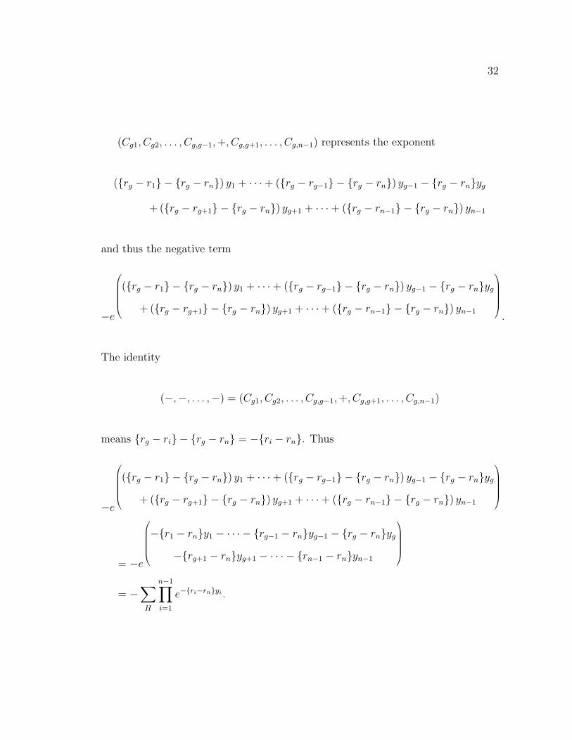
(Cg1, Cg2, . . . , Cg,g−1, +, Cg,g+1, . . . , Cg,n−1) represents the exponent
(rg − r1 − rg − rn) y1 + · · ·+ (rg − rg−1 − rg − rn) yg−1 − rg − rnyg
+ (rg − rg+1 − rg − rn) yg+1 + · · ·+ (rg − rn−1 − rg − rn) yn−1
and thus the negative term
−e
0BBBB@(rg − r1 − rg − rn) y1 + · · ·+ (rg − rg−1 − rg − rn) yg−1 − rg − rnyg
+ (rg − rg+1 − rg − rn) yg+1 + · · ·+ (rg − rn−1 − rg − rn) yn−1
1CCCCA.
The identity
(−,−, . . . ,−) = (Cg1, Cg2, . . . , Cg,g−1, +, Cg,g+1, . . . , Cg,n−1)
means rg − ri − rg − rn = −ri − rn. Thus
−e
0BBBB@(rg − r1 − rg − rn) y1 + · · ·+ (rg − rg−1 − rg − rn) yg−1 − rg − rnyg
+ (rg − rg+1 − rg − rn) yg+1 + · · ·+ (rg − rn−1 − rg − rn) yn−1
1CCCCA
= −e
0BBBB@−r1 − rny1 − · · · − rg−1 − rnyg−1 − rg − rnyg
−rg+1 − rnyg+1 − · · · − rn−1 − rnyn−1
1CCCCA
= −∑H
n−1∏i=1
e−ri−rnyi .
33
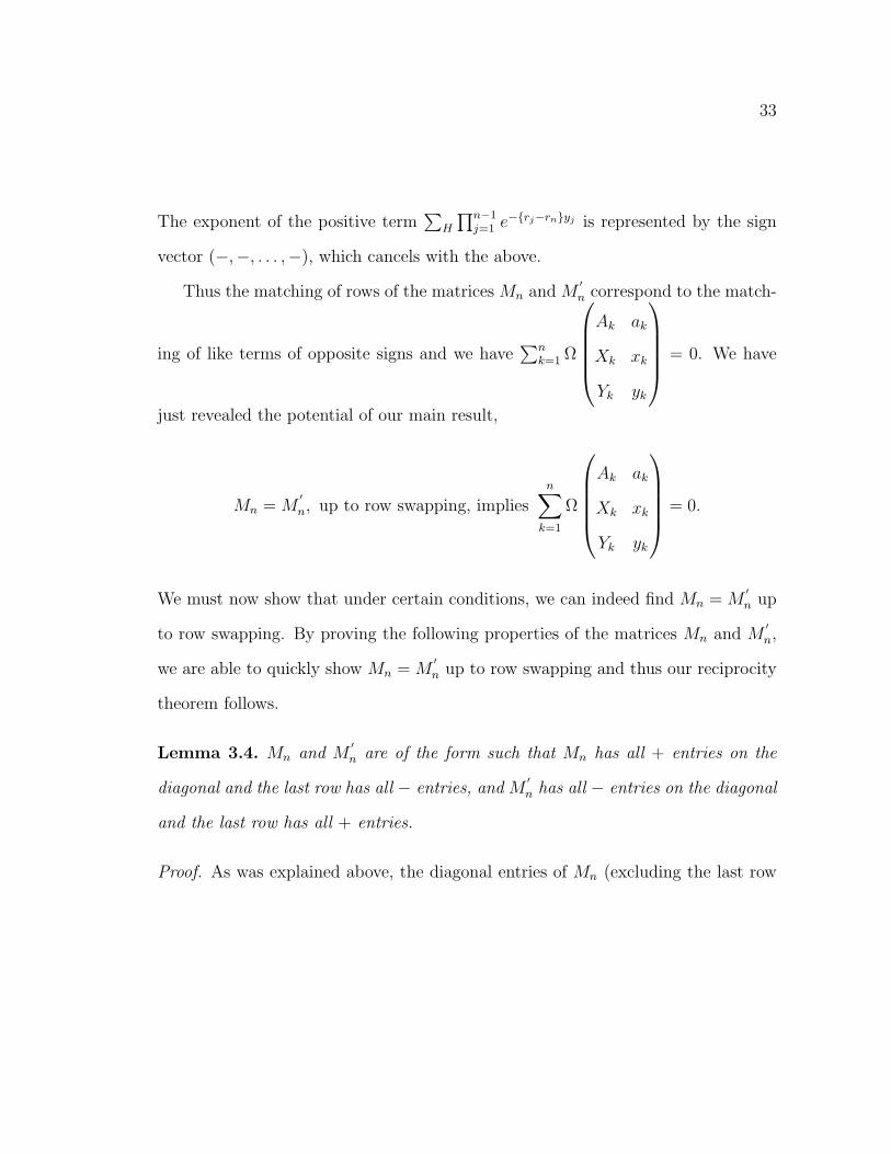
The exponent of the positive term∑
H
∏n−1j=1 e−rj−rnyj is represented by the sign
vector (−,−, . . . ,−), which cancels with the above.
Thus the matching of rows of the matrices Mn and M′n correspond to the match-
ing of like terms of opposite signs and we have∑n
k=1 Ω
Ak ak
Xk xk
Yk yk
= 0. We have
just revealed the potential of our main result,
Mn = M′
n, up to row swapping, impliesn∑
k=1
Ω
Ak ak
Xk xk
Yk yk
= 0.
We must now show that under certain conditions, we can indeed find Mn = M′n up
to row swapping. By proving the following properties of the matrices Mn and M′n,
we are able to quickly show Mn = M′n up to row swapping and thus our reciprocity
theorem follows.
Lemma 3.4. Mn and M′n are of the form such that Mn has all + entries on the
diagonal and the last row has all − entries, and M′n has all − entries on the diagonal
and the last row has all + entries.
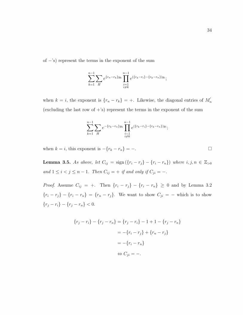
Proof. As was explained above, the diagonal entries of Mn (excluding the last row
34
of −’s) represent the terms in the exponent of the sum
n−1∑k=1
∑H
ern−rkyk
n−1∏i=1i6=k
e(rk−ri−rk−rn)yi ;
when k = i, the exponent is rn − rk = +. Likewise, the diagonal entries of M′n
(excluding the last row of +’s) represent the terms in the exponent of the sum
n−1∑k=1
∑H
e−rk−rnyk
n−1∏i=1i6=k
e(rk−ri−rk−rn)yi ;
when k = i, this exponent is −rk − rn = −.
Lemma 3.5. As above, let Cij = sign (ri − rj − ri − rn) where i, j, n ∈ Z>0
and 1 ≤ i < j ≤ n− 1. Then Cij = + if and only if Cji = −.
Proof. Assume Cij = +. Then ri − rj − ri − rn ≥ 0 and by Lemma 3.2
ri − rj − ri − rn = rn − rj. We want to show Cji = − which is to show
rj − ri − rj − rn < 0.
rj − ri − rj − rn = rj − ri − 1 + 1− rj − rn
= −ri − rj+ rn − rj
= −ri − rn
⇔ Cji = −.
35
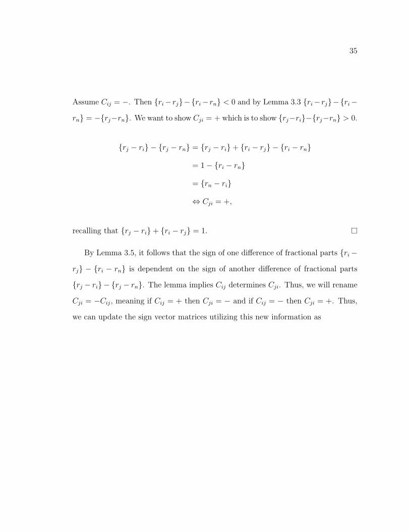
Assume Cij = −. Then ri− rj−ri− rn < 0 and by Lemma 3.3 ri− rj−ri−
rn = −rj−rn. We want to show Cji = + which is to show rj−ri−rj−rn > 0.
rj − ri − rj − rn = rj − ri+ ri − rj − ri − rn
= 1− ri − rn
= rn − ri
⇔ Cji = +,
recalling that rj − ri+ ri − rj = 1.
By Lemma 3.5, it follows that the sign of one difference of fractional parts ri −
rj − ri − rn is dependent on the sign of another difference of fractional parts
rj − ri− rj − rn. The lemma implies Cij determines Cji. Thus, we will rename
Cji = −Cij, meaning if Cij = + then Cji = − and if Cij = − then Cji = +. Thus,
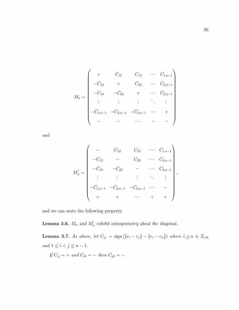
we can update the sign vector matrices utilizing this new information as
36
Mn =
+ C12 C13 · · · C1,n−1
−C12 + C23 · · · C2,n−1
−C13 −C23 + · · · C3,n−1
......
.... . .
...
−C1,n−1 −C2,n−1 −C3,n−1 · · · +
− − · · · − −
and
M′
n =
− C12 C13 · · · C1,n−1
−C12 − C23 · · · C2,n−1
−C13 −C23 − · · · C3,n−1
......
.... . .
...
−C1,n−1 −C2,n−1 −C3,n−1 · · · −
+ + · · · + +
,
and we can state the following property.
Lemma 3.6. Mn and M′n exhibit antisymmetry about the diagonal.
Lemma 3.7. As above, let Cij = sign (ri − rj − ri − rn) where i, j, n ∈ Z>0
and 1 ≤ i < j ≤ n− 1.
If Cij = + and Cik = − then Cjk = −.
37
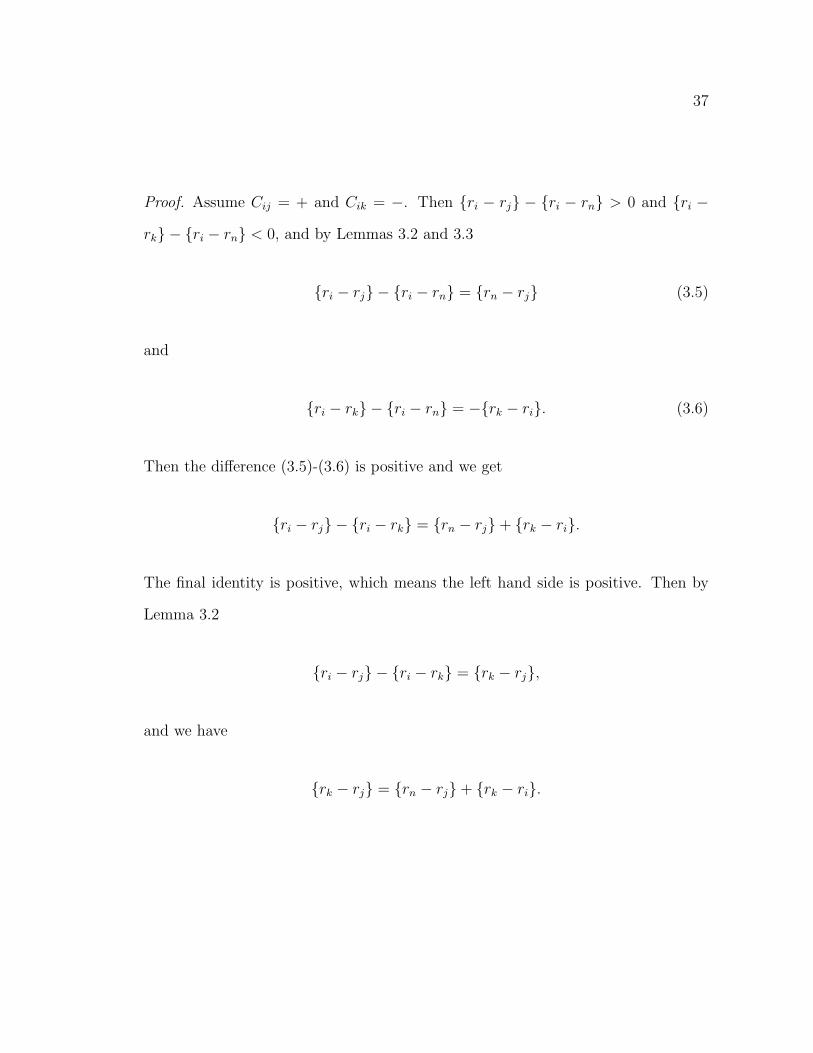
Proof. Assume Cij = + and Cik = −. Then ri − rj − ri − rn > 0 and ri −
rk − ri − rn < 0, and by Lemmas 3.2 and 3.3
ri − rj − ri − rn = rn − rj (3.5)
and
ri − rk − ri − rn = −rk − ri. (3.6)
Then the difference (3.5)-(3.6) is positive and we get
ri − rj − ri − rk = rn − rj+ rk − ri.
The final identity is positive, which means the left hand side is positive. Then by
Lemma 3.2
ri − rj − ri − rk = rk − rj,
and we have
rk − rj = rn − rj+ rk − ri.
38
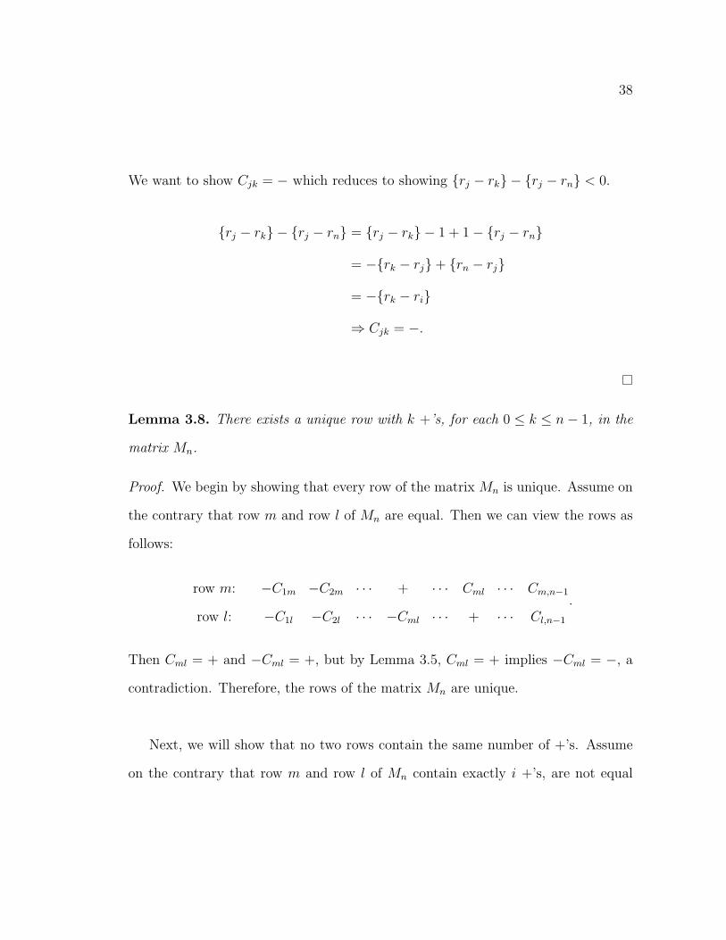
We want to show Cjk = − which reduces to showing rj − rk − rj − rn < 0.
rj − rk − rj − rn = rj − rk − 1 + 1− rj − rn
= −rk − rj+ rn − rj
= −rk − ri
⇒ Cjk = −.
Lemma 3.8. There exists a unique row with k +’s, for each 0 ≤ k ≤ n− 1, in the
matrix Mn.
Proof. We begin by showing that every row of the matrix Mn is unique. Assume on
the contrary that row m and row l of Mn are equal. Then we can view the rows as
follows:
row m: −C1m −C2m · · · + · · · Cml · · · Cm,n−1
row l: −C1l −C2l · · · −Cml · · · + · · · Cl,n−1
.
Then Cml = + and −Cml = +, but by Lemma 3.5, Cml = + implies −Cml = −, a
contradiction. Therefore, the rows of the matrix Mn are unique.
Next, we will show that no two rows contain the same number of +’s. Assume
on the contrary that row m and row l of Mn contain exactly i +’s, are not equal
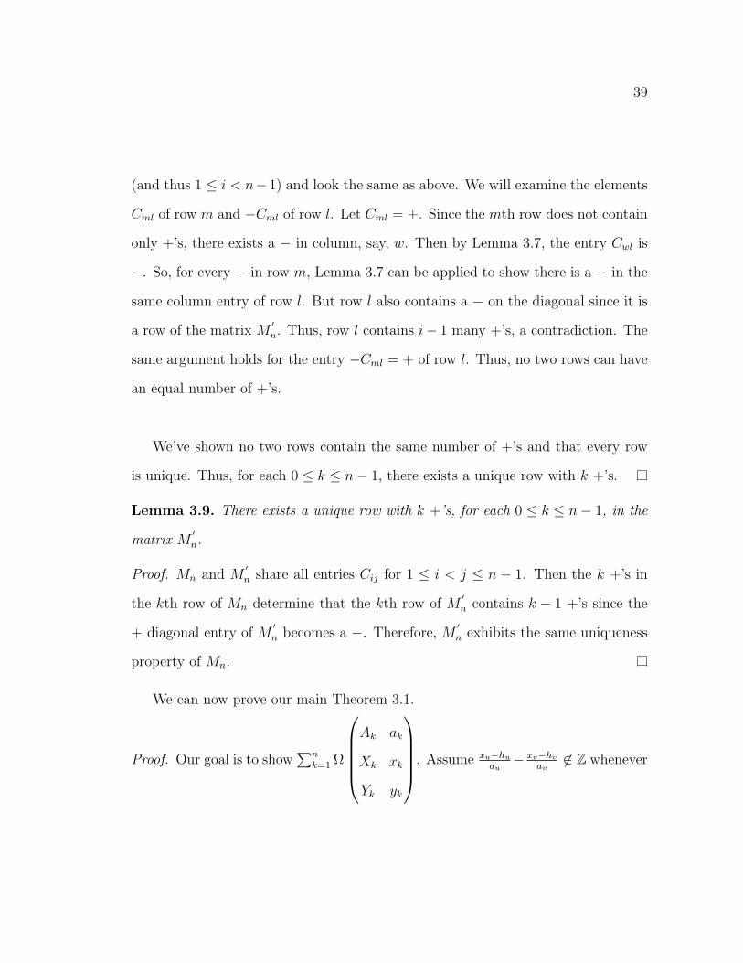
39
(and thus 1 ≤ i < n−1) and look the same as above. We will examine the elements
Cml of row m and −Cml of row l. Let Cml = +. Since the mth row does not contain
only +’s, there exists a − in column, say, w. Then by Lemma 3.7, the entry Cwl is
−. So, for every − in row m, Lemma 3.7 can be applied to show there is a − in the
same column entry of row l. But row l also contains a − on the diagonal since it is
a row of the matrix M′n. Thus, row l contains i− 1 many +’s, a contradiction. The
same argument holds for the entry −Cml = + of row l. Thus, no two rows can have
an equal number of +’s.
We’ve shown no two rows contain the same number of +’s and that every row
is unique. Thus, for each 0 ≤ k ≤ n− 1, there exists a unique row with k +’s.
Lemma 3.9. There exists a unique row with k +’s, for each 0 ≤ k ≤ n− 1, in the
matrix M′n.
Proof. Mn and M′n share all entries Cij for 1 ≤ i < j ≤ n − 1. Then the k +’s in
the kth row of Mn determine that the kth row of M′n contains k − 1 +’s since the
+ diagonal entry of M′n becomes a −. Therefore, M
′n exhibits the same uniqueness
property of Mn.
We can now prove our main Theorem 3.1.
Proof. Our goal is to show∑n
k=1 Ω
Ak ak
Xk xk
Yk yk
. Assume xu−hu
au− xv−hv
av6∈ Z whenever
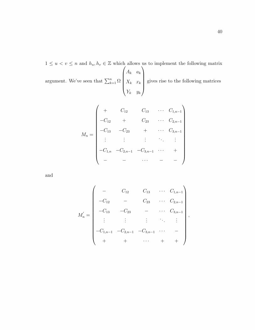
40
1 ≤ u < v ≤ n and hu, hv ∈ Z which allows us to implement the following matrix
argument. We’ve seen that∑n
k=1 Ω
Ak ak
Xk xk
Yk yk
gives rise to the following matrices
Mn =
+ C12 C13 · · · C1,n−1
−C12 + C23 · · · C2,n−1
−C13 −C23 + · · · C3,n−1
......
.... . .
...
−C1,n −C2,n−1 −C3,n−1 · · · +
− − · · · − −
and
M′
n =
− C12 C13 · · · C1,n−1
−C12 − C23 · · · C2,n−1
−C13 −C23 − · · · C3,n−1
......
.... . .
...
−C1,n−1 −C2,n−1 −C3,n−1 · · · −
+ + · · · + +
,
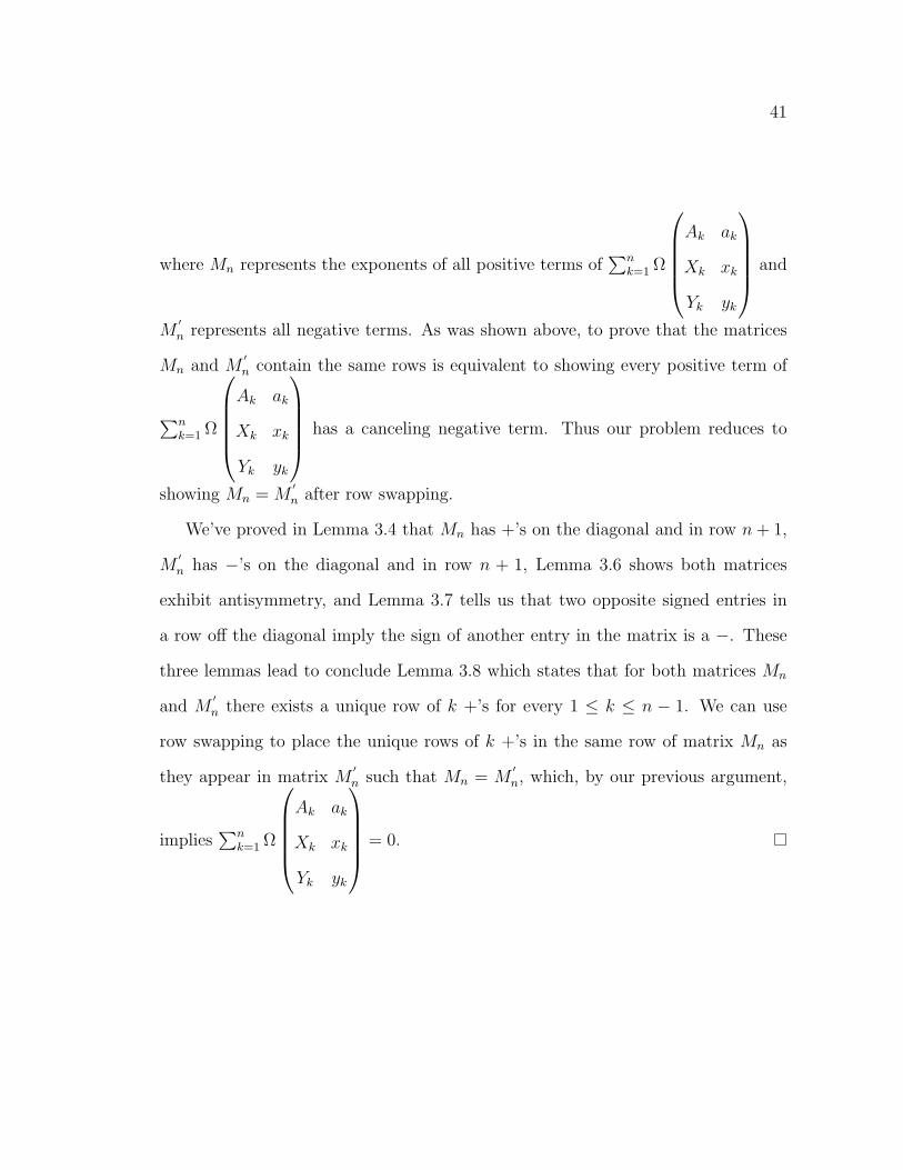
41
where Mn represents the exponents of all positive terms of∑n
k=1 Ω
Ak ak
Xk xk
Yk yk
and
M′n represents all negative terms. As was shown above, to prove that the matrices
Mn and M′n contain the same rows is equivalent to showing every positive term of
∑nk=1 Ω
Ak ak
Xk xk
Yk yk
has a canceling negative term. Thus our problem reduces to
showing Mn = M′n after row swapping.
We’ve proved in Lemma 3.4 that Mn has +’s on the diagonal and in row n + 1,
M′n has −’s on the diagonal and in row n + 1, Lemma 3.6 shows both matrices
exhibit antisymmetry, and Lemma 3.7 tells us that two opposite signed entries in
a row off the diagonal imply the sign of another entry in the matrix is a −. These
three lemmas lead to conclude Lemma 3.8 which states that for both matrices Mn
and M′n there exists a unique row of k +’s for every 1 ≤ k ≤ n − 1. We can use
row swapping to place the unique rows of k +’s in the same row of matrix Mn as
they appear in matrix M′n such that Mn = M
′n, which, by our previous argument,
implies∑n
k=1 Ω
Ak ak
Xk xk
Yk yk
= 0.
Chapter 4
A New Proof of Hall–Wilson–Zagier’s
Reciprocity Theorem
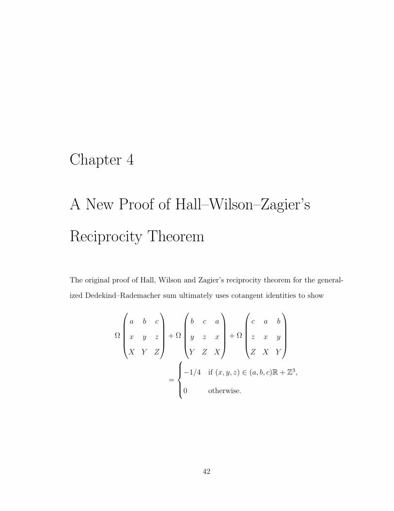
The original proof of Hall, Wilson and Zagier’s reciprocity theorem for the general-
ized Dedekind–Rademacher sum ultimately uses cotangent identities to show
Ω
a b c
x y z
X Y Z
+ Ω
b c a
y z x
Y Z X
+ Ω
c a b
z x y
Z X Y
=
−1/4 if (x, y, z) ∈ (a, b, c)R + Z3,
0 otherwise.
42
43
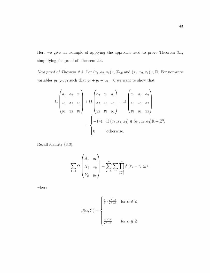
Here we give an example of applying the approach used to prove Theorem 3.1,
simplifying the proof of Theorem 2.4.
New proof of Theorem 2.4. Let (a1, a2, a3) ∈ Z>0 and (x1, x2, x3) ∈ R. For non-zero
variables y1, y2, y3 such that y1 + y2 + y3 = 0 we want to show that
Ω
a1 a2 a3
x1 x2 x3
y1 y2 y3
+ Ω
a2 a3 a1
x2 x3 x1
y2 y3 y1
+ Ω
a3 a1 a2
x3 x1 x2
y3 y1 y2
=
−1/4 if (x1, x2, x3) ∈ (a1, a2, a3)R + Z3,
0 otherwise.
Recall identity (3.3),
n∑k=1
Ω
Ak ak
Xk xk
Yk yk
=n∑
k=1
∑H
n∏i=1i6=k
β (rk − ri, yi) ,
where
β(α, Y ) =
12· eY +1
eY −1for α ∈ Z,
eαY
eY −1for α 6∈ Z,
44
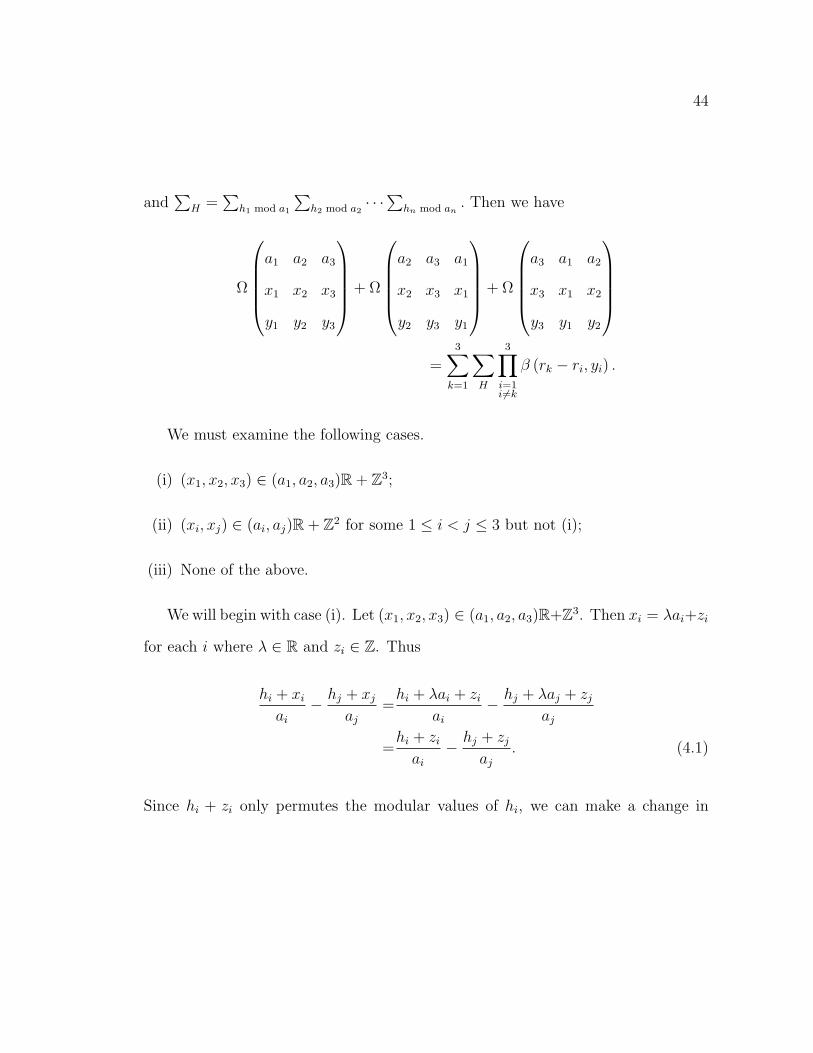
and∑
H =∑
h1 mod a1
∑h2 mod a2
· · ·∑
hn mod an. Then we have
Ω
a1 a2 a3
x1 x2 x3
y1 y2 y3
+ Ω
a2 a3 a1
x2 x3 x1
y2 y3 y1
+ Ω
a3 a1 a2
x3 x1 x2
y3 y1 y2
=
3∑k=1
∑H
3∏i=1i6=k
β (rk − ri, yi) .
We must examine the following cases.
(i) (x1, x2, x3) ∈ (a1, a2, a3)R + Z3;
(ii) (xi, xj) ∈ (ai, aj)R + Z2 for some 1 ≤ i < j ≤ 3 but not (i);
(iii) None of the above.
We will begin with case (i). Let (x1, x2, x3) ∈ (a1, a2, a3)R+Z3. Then xi = λai+zi
for each i where λ ∈ R and zi ∈ Z. Thus
hi + xi
ai
− hj + xj
aj
=hi + λai + zi
ai
− hj + λaj + zj
aj
=hi + zi
ai
− hj + zj
aj
. (4.1)
Since hi + zi only permutes the modular values of hi, we can make a change in
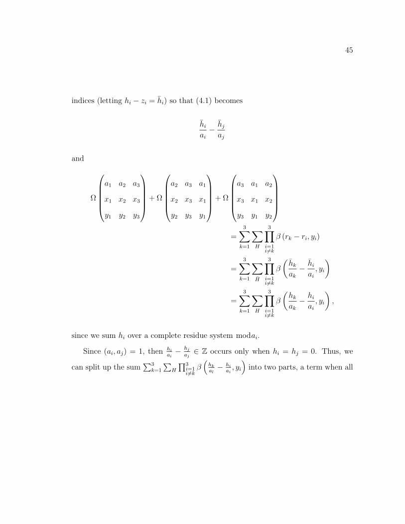
45
indices (letting hi − zi = hi) so that (4.1) becomes
hi
ai
− hj
aj
and
Ω
a1 a2 a3
x1 x2 x3
y1 y2 y3
+ Ω
a2 a3 a1
x2 x3 x1
y2 y3 y1
+ Ω
a3 a1 a2
x3 x1 x2
y3 y1 y2
=
3∑k=1
∑H
3∏i=1i6=k
β (rk − ri, yi)
=3∑
k=1
∑H
3∏i=1i6=k
β
(hk
ak
− hi
ai
, yi
)
=3∑
k=1
∑H
3∏i=1i6=k
β
(hk
ak
− hi
ai
, yi
),
since we sum hi over a complete residue system modai.
Since (ai, aj) = 1, then hi
ai− hj
aj∈ Z occurs only when hi = hj = 0. Thus, we
can split up the sum∑3
k=1
∑H
∏3i=1i6=k
β(
hk
al− hi
ai, yi
)into two parts, a term when all
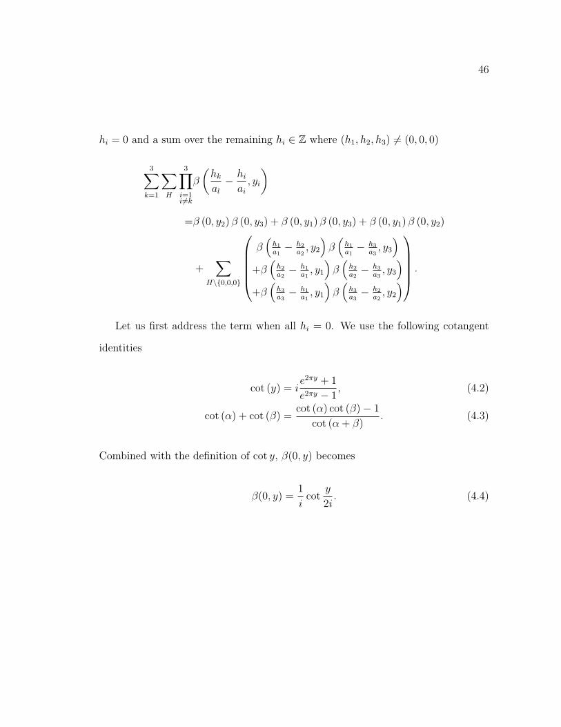
46
hi = 0 and a sum over the remaining hi ∈ Z where (h1, h2, h3) 6= (0, 0, 0)
3∑k=1
∑H
3∏i=1i6=k
β
(hk
al
− hi
ai
, yi
)
=β (0, y2) β (0, y3) + β (0, y1) β (0, y3) + β (0, y1) β (0, y2)
+∑
H\0,0,0
β
(h1
a1− h2
a2, y2
)β
(h1
a1− h3
a3, y3
)+β
(h2
a2− h1
a1, y1
)β
(h2
a2− h3
a3, y3
)+β
(h3
a3− h1
a1, y1
)β
(h3
a3− h2
a2, y2
) .
Let us first address the term when all hi = 0. We use the following cotangent
identities
cot (y) = ie2πy + 1
e2πy − 1, (4.2)
cot (α) + cot (β) =cot (α) cot (β)− 1
cot (α + β). (4.3)
Combined with the definition of cot y, β(0, y) becomes
β(0, y) =1
icot
y
2i. (4.4)
47
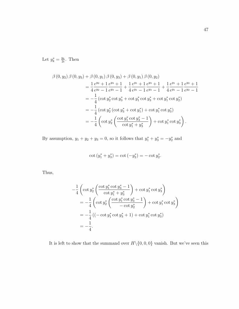
Let y∗k = yk
2i. Then
β (0, y2) β (0, y3) + β (0, y1) β (0, y3) + β (0, y1) β (0, y2)
=1
4
ey2 + 1
ey2 − 1
ey3 + 1
ey3 − 1+
1
4
ey1 + 1
ey1 − 1
ey3 + 1
ey3 − 1+
1
4
ey1 + 1
ey1 − 1
ey2 + 1
ey2 − 1
= −1
4(cot y∗2 cot y∗3 + cot y∗1 cot y∗3 + cot y∗1 cot y∗2)
= −1
4(cot y∗2 (cot y∗3 + cot y∗1) + cot y∗1 cot y∗3)
= −1
4
(cot y∗2
(cot y∗1 cot y∗3 − 1
cot y∗1 + y∗3
)+ cot y∗1 cot y∗3
).
By assumption, y1 + y2 + y3 = 0, so it follows that y∗1 + y∗3 = −y∗2 and
cot (y∗1 + y∗3) = cot (−y∗2) = − cot y∗2.
Thus,
−1
4
(cot y∗2
(cot y∗1 cot y∗3 − 1
cot y∗1 + y∗3
)+ cot y∗1 cot y∗3
)= −1
4
(cot y∗2
(cot y∗1 cot y∗3 − 1
− cot y∗2
)+ cot y∗1 cot y∗3
)= −1
4((− cot y∗1 cot y∗3 + 1) + cot y∗1 cot y∗3)
= −1
4.
It is left to show that the summand over H\0, 0, 0 vanish. But we’ve seen this
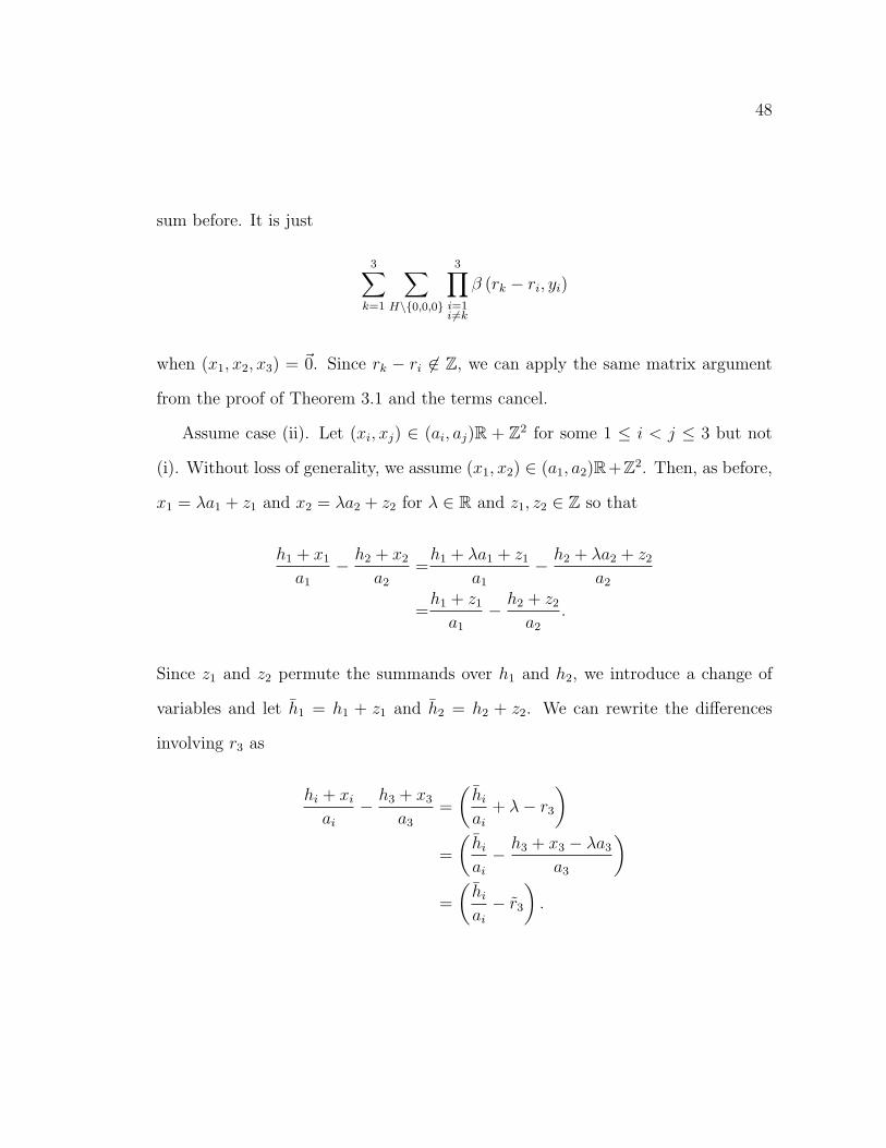
48
sum before. It is just
3∑k=1
∑H\0,0,0
3∏i=1i6=k
β (rk − ri, yi)
when (x1, x2, x3) = ~0. Since rk − ri 6∈ Z, we can apply the same matrix argument
from the proof of Theorem 3.1 and the terms cancel.
Assume case (ii). Let (xi, xj) ∈ (ai, aj)R + Z2 for some 1 ≤ i < j ≤ 3 but not
(i). Without loss of generality, we assume (x1, x2) ∈ (a1, a2)R+Z2. Then, as before,
x1 = λa1 + z1 and x2 = λa2 + z2 for λ ∈ R and z1, z2 ∈ Z so that
h1 + x1
a1
− h2 + x2
a2
=h1 + λa1 + z1
a1
− h2 + λa2 + z2
a2
=h1 + z1
a1
− h2 + z2
a2
.
Since z1 and z2 permute the summands over h1 and h2, we introduce a change of
variables and let h1 = h1 + z1 and h2 = h2 + z2. We can rewrite the differences
involving r3 as
hi + xi
ai
− h3 + x3
a3
=
(hi
ai
+ λ− r3
)=
(hi
ai
− h3 + x3 − λa3
a3
)=
(hi
ai
− r3
).
49
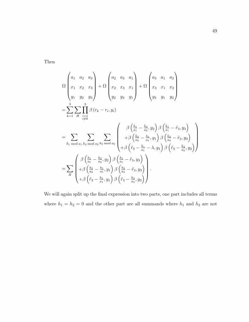
Then
Ω
a1 a2 a3
x1 x2 x3
y1 y2 y3
+ Ω
a2 a3 a1
x2 x3 x1
y2 y3 y1
+ Ω
a3 a1 a2
x3 x1 x2
y3 y1 y2
=
3∑k=1
∑H
3∏i=1i6=k
β (rk − ri, yi)
=∑
h1 mod a1
∑h2 mod a2
∑h3 mod a3
β
(h1
a1− h2
a2, y2
)β
(h1
a1− r3, y3
)+β
(h2
a2− h1
a1, y1
)β
(h2
a2− r3, y3
)+β
(r3 − h1
a1− λ, y1
)β
(r3 − h2
a2, y2
)
=∑H
β
(h1
a1− h2
a2, y2
)β
(h1
a1− r3, y3
)+β
(h2
a2− h1
a1, y1
)β
(h2
a2− r3, y3
)+β
(r3 − h1
a1, y1
)β
(r3 − h2
a2, y2
) .
We will again split up the final expression into two parts, one part includes all terms
where h1 = h2 = 0 and the other part are all summands where h1 and h2 are not
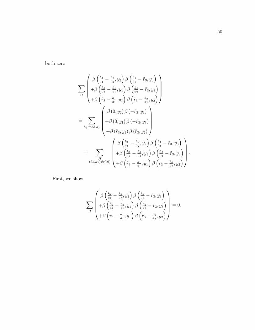
50
both zero
∑H
β
(h1
a1− h2
a2, y2
)β
(h1
a1− r3, y3
)+β
(h2
a2− h1
a1, y1
)β
(h2
a2− r3, y3
)+β
(r3 − h1
a1, y1
)β
(r3 − h2
a2, y2
)
=∑
h3 mod a3
β (0, y2) β (−r3, y3)
+β (0, y1) β (−r3, y3)
+β (r3, y1) β (r3, y2)
+∑H
(h1,h2) 6=(0,0)
β
(h1
a1− h2
a2, y2
)β
(h1
a1− r3, y3
)+β
(h2
a2− h1
a1, y1
)β
(h2
a2− r3, y3
)+β
(r3 − h1
a1, y1
)β
(r3 − h2
a2, y2
) .
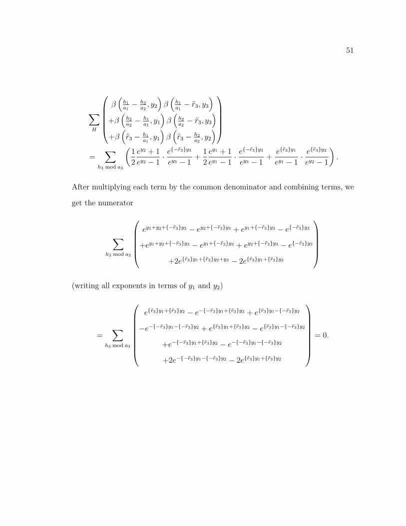
First, we show
∑H
β
(h1
a1− h2
a2, y2
)β
(h1
a1− r3, y3
)+β
(h2
a2− h1
a1, y1
)β
(h2
a2− r3, y3
)+β
(r3 − h1
a1, y1
)β
(r3 − h2
a2, y2
) = 0.
51
∑H
β
(h1
a1− h2
a2, y2
)β
(h1
a1− r3, y3
)+β
(h2
a2− h1
a1, y1
)β
(h2
a2− r3, y3
)+β
(r3 − h1
a1, y1
)β
(r3 − h2
a2, y2
)
=∑
h3 mod a3
(1
2
ey2 + 1
ey2 − 1· e−r3y3
ey3 − 1+
1
2
ey1 + 1
ey1 − 1· e−r3y3
ey3 − 1+
er3y1
ey1 − 1· er3y2
ey2 − 1
).
After multiplying each term by the common denominator and combining terms, we
get the numerator
∑h3 mod a3
ey1+y2+−r3y3 − ey2+−r3y3 + ey1+−r3y3 − e−r3y3
+ey1+y2+−r3y3 − ey1+−r3y3 + ey2+−r3y3 − e−r3y3
+2er3y1+r3y2+y3 − 2er3y1+r3y2
(writing all exponents in terms of y1 and y2)
=∑
h3 mod a3
er3y1+r3y2 − e−−r3y1+r3y2 + er3y1−−r3y2
−e−−r3y1−−r3y2 + er3y1+r3y2 − er3y1−−r3y2
+e−−r3y1+r3y2 − e−−r3y1−−r3y2
+2e−−r3y1−−r3y2 − 2er3y1+r3y2
= 0.
52
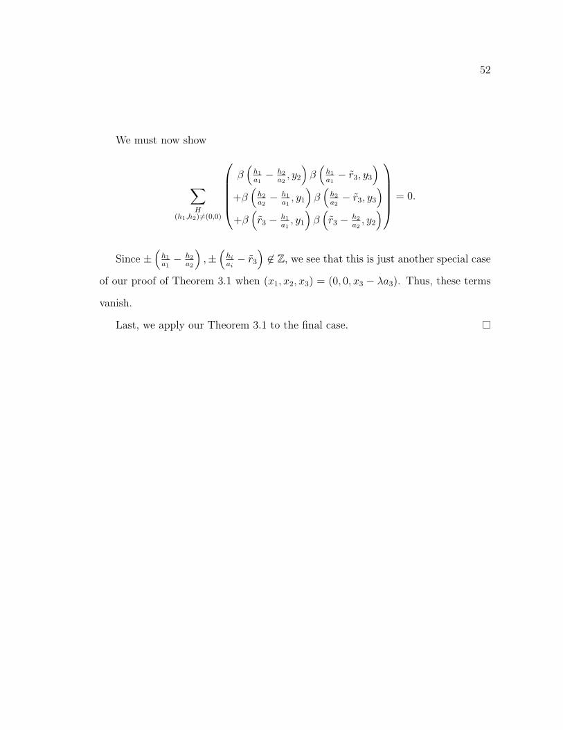
We must now show
∑H
(h1,h2) 6=(0,0)
β
(h1
a1− h2
a2, y2
)β
(h1
a1− r3, y3
)+β
(h2
a2− h1
a1, y1
)β
(h2
a2− r3, y3
)+β
(r3 − h1
a1, y1
)β
(r3 − h2
a2, y2
) = 0.
Since ±(
h1
a1− h2
a2
),±
(hi
ai− r3
)6∈ Z, we see that this is just another special case
of our proof of Theorem 3.1 when (x1, x2, x3) = (0, 0, x3 − λa3). Thus, these terms
vanish.
Last, we apply our Theorem 3.1 to the final case.
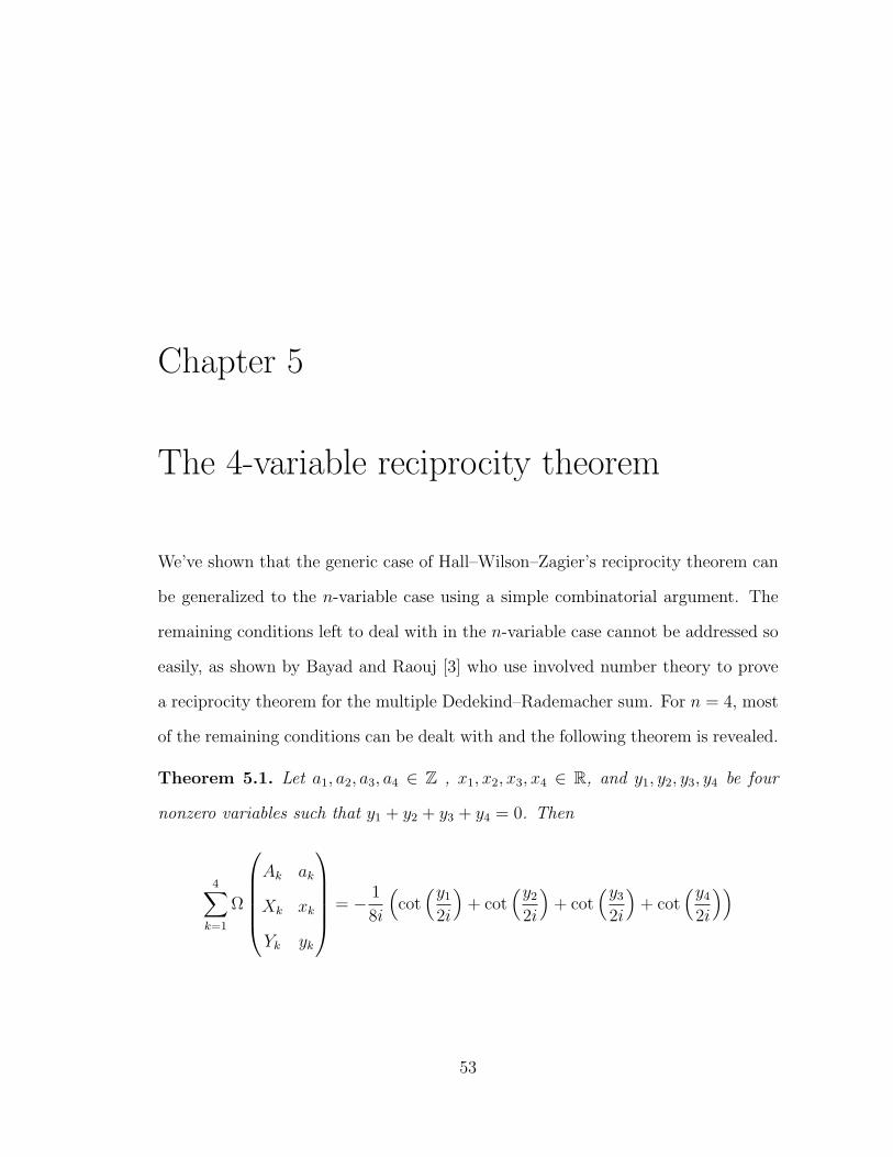
Chapter 5
The 4-variable reciprocity theorem
We’ve shown that the generic case of Hall–Wilson–Zagier’s reciprocity theorem can
be generalized to the n-variable case using a simple combinatorial argument. The
remaining conditions left to deal with in the n-variable case cannot be addressed so
easily, as shown by Bayad and Raouj [3] who use involved number theory to prove
a reciprocity theorem for the multiple Dedekind–Rademacher sum. For n = 4, most
of the remaining conditions can be dealt with and the following theorem is revealed.
Theorem 5.1. Let a1, a2, a3, a4 ∈ Z , x1, x2, x3, x4 ∈ R, and y1, y2, y3, y4 be four
nonzero variables such that y1 + y2 + y3 + y4 = 0. Then
4∑k=1
Ω
Ak ak
Xk xk
Yk yk
= − 1
8i
(cot
(y1
2i
)+ cot
(y2
2i
)+ cot
(y3
2i
)+ cot
(y4
2i
))
53
54
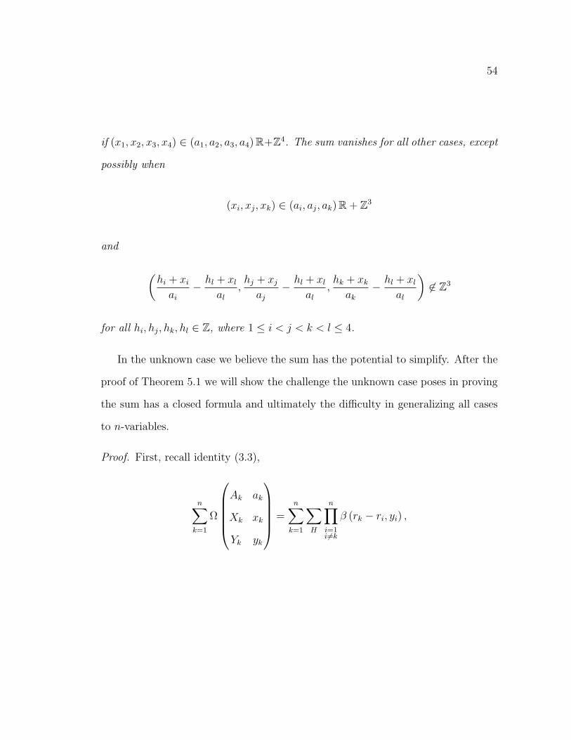
if (x1, x2, x3, x4) ∈ (a1, a2, a3, a4) R+Z4. The sum vanishes for all other cases, except
possibly when
(xi, xj, xk) ∈ (ai, aj, ak) R + Z3
and
(hi + xi
ai
− hl + xl
al
,hj + xj
aj
− hl + xl
al
,hk + xk
ak
− hl + xl
al
)6∈ Z3
for all hi, hj, hk, hl ∈ Z, where 1 ≤ i < j < k < l ≤ 4.
In the unknown case we believe the sum has the potential to simplify. After the
proof of Theorem 5.1 we will show the challenge the unknown case poses in proving
the sum has a closed formula and ultimately the difficulty in generalizing all cases
to n-variables.
Proof. First, recall identity (3.3),
n∑k=1
Ω
Ak ak
Xk xk
Yk yk
=n∑
k=1
∑H
n∏i=1i6=k
β (rk − ri, yi) ,
55
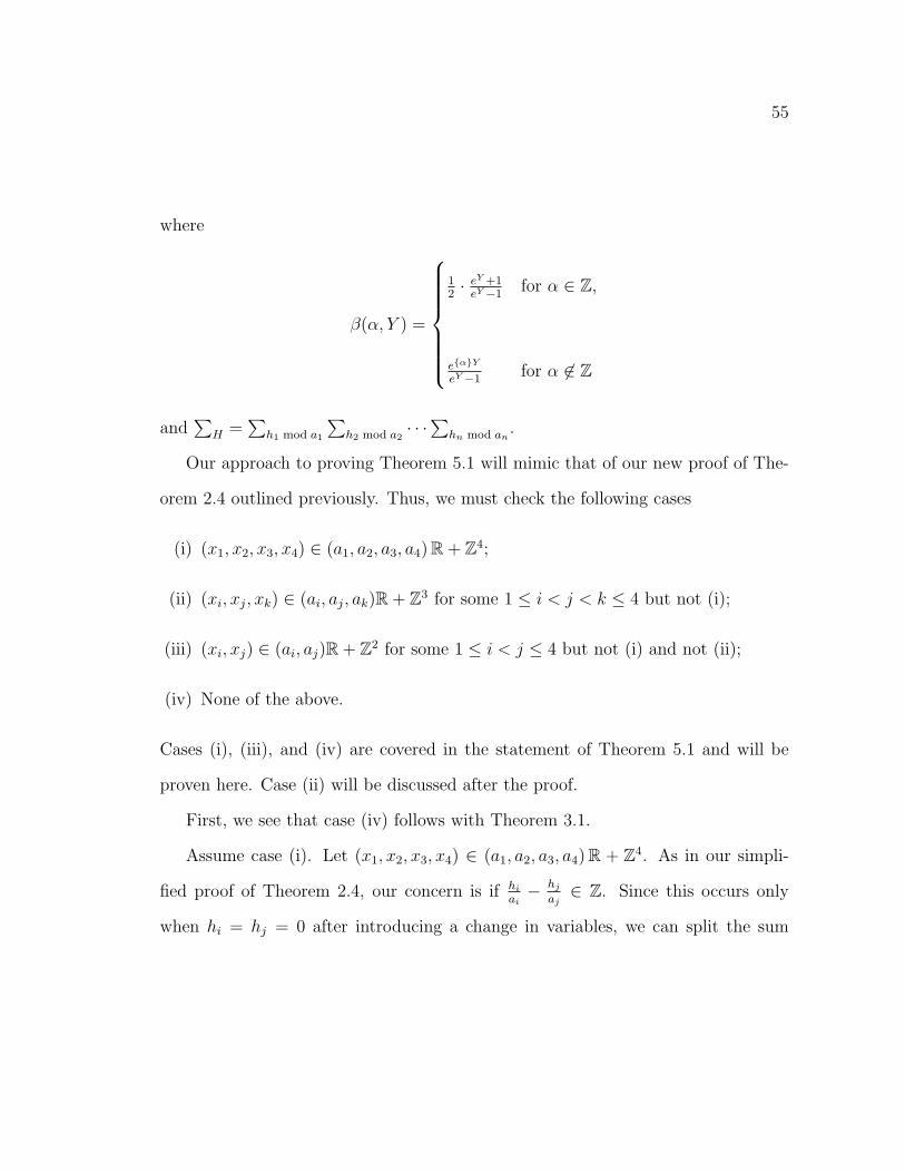
where
β(α, Y ) =
12· eY +1
eY −1for α ∈ Z,
eαY
eY −1for α 6∈ Z
and∑
H =∑
h1 mod a1
∑h2 mod a2
· · ·∑
hn mod an.
Our approach to proving Theorem 5.1 will mimic that of our new proof of The-
orem 2.4 outlined previously. Thus, we must check the following cases
(i) (x1, x2, x3, x4) ∈ (a1, a2, a3, a4) R + Z4;
(ii) (xi, xj, xk) ∈ (ai, aj, ak)R + Z3 for some 1 ≤ i < j < k ≤ 4 but not (i);
(iii) (xi, xj) ∈ (ai, aj)R + Z2 for some 1 ≤ i < j ≤ 4 but not (i) and not (ii);
(iv) None of the above.
Cases (i), (iii), and (iv) are covered in the statement of Theorem 5.1 and will be
proven here. Case (ii) will be discussed after the proof.
First, we see that case (iv) follows with Theorem 3.1.
Assume case (i). Let (x1, x2, x3, x4) ∈ (a1, a2, a3, a4) R + Z4. As in our simpli-
fied proof of Theorem 2.4, our concern is if hi
ai− hj
aj∈ Z. Since this occurs only
when hi = hj = 0 after introducing a change in variables, we can split the sum
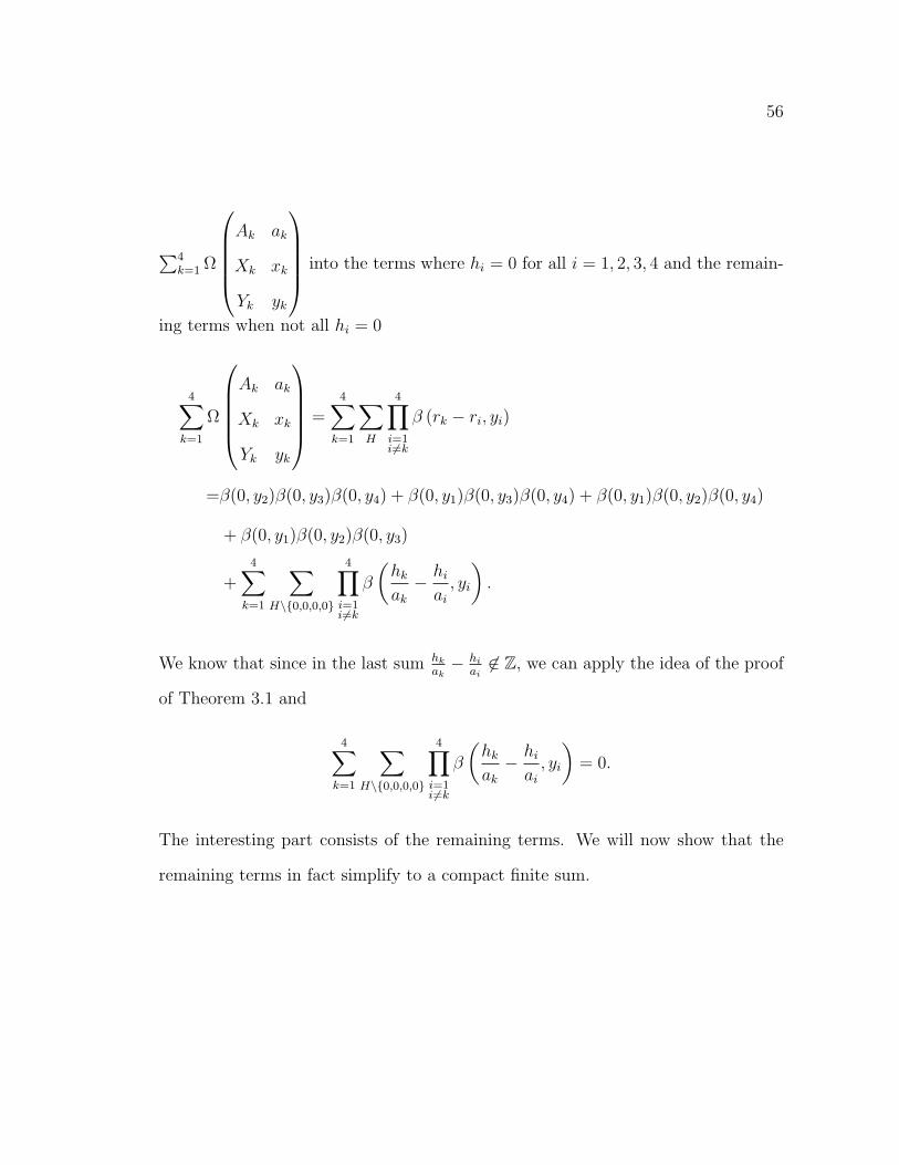
56
∑4k=1 Ω
Ak ak
Xk xk
Yk yk
into the terms where hi = 0 for all i = 1, 2, 3, 4 and the remain-
ing terms when not all hi = 0
4∑k=1
Ω
Ak ak
Xk xk
Yk yk
=4∑
k=1
∑H
4∏i=1i6=k
β (rk − ri, yi)
=β(0, y2)β(0, y3)β(0, y4) + β(0, y1)β(0, y3)β(0, y4) + β(0, y1)β(0, y2)β(0, y4)
+ β(0, y1)β(0, y2)β(0, y3)
+4∑
k=1
∑H\0,0,0,0
4∏i=1i6=k
β
(hk
ak
− hi
ai
, yi
).
We know that since in the last sum hk
ak− hi
ai6∈ Z, we can apply the idea of the proof
of Theorem 3.1 and
4∑k=1
∑H\0,0,0,0
4∏i=1i6=k
β
(hk
ak
− hi
ai
, yi
)= 0.
The interesting part consists of the remaining terms. We will now show that the
remaining terms in fact simplify to a compact finite sum.
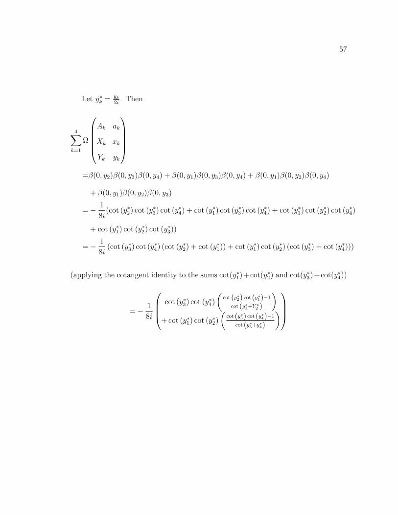
57
Let y∗k = yk
2i. Then
4∑k=1
Ω
Ak ak
Xk xk
Yk yk
=β(0, y2)β(0, y3)β(0, y4) + β(0, y1)β(0, y3)β(0, y4) + β(0, y1)β(0, y2)β(0, y4)
+ β(0, y1)β(0, y2)β(0, y3)
=− 1
8i(cot (y∗2) cot (y∗3) cot (y∗4) + cot (y∗1) cot (y∗3) cot (y∗4) + cot (y∗1) cot (y∗2) cot (y∗4)
+ cot (y∗1) cot (y∗2) cot (y∗3))
=− 1
8i(cot (y∗3) cot (y∗4) (cot (y∗2) + cot (y∗1)) + cot (y∗1) cot (y∗2) (cot (y∗3) + cot (y∗4)))
(applying the cotangent identity to the sums cot(y∗1)+cot(y∗2) and cot(y∗3)+cot(y∗4))
=− 1
8i
cot (y∗3) cot (y∗4)
(cot (y∗2) cot (y∗1)−1
cot (y∗1+Y ∗2 )
)+ cot (y∗1) cot (y∗2)
(cot (y∗3) cot (y∗4)−1
cot (y∗3+y∗4)
)

58
(since y1 + y2 + y3 + y4 = 0, then cot (y∗3 + y∗4) = cot (−y∗1 − y∗2) = − cot (y∗1 + y∗2))
=− 1
8i·
cot (y3∗) cot (y∗4) (cot (y∗2) cot (y∗1)− 1)
− cot (y∗1) cot (y∗2) (cot (y∗3) cot (y∗4)− 1)
cot (y∗1 + y∗2)
=− 1
8i(cot (y∗1) cot (y∗2)− cot (y∗3) cot (y∗4))
(solving the cotangent identity for cot(α)cot(β), we apply this identity to both
cotangent products in the sum above)
=− 1
8i·
cot (y∗1 + y∗2) (cot (y∗2) + cot (y∗1)) + 1
− cot (y∗3 + y∗4) (cot (y∗3) + cot (y∗4))− 1
cot (y∗1 + y∗2)
=− 1
8i·
cot (y∗1 + y∗2) (cot (y∗2) + cot (y∗1)) + 1
+ cot (y∗1 + y∗2) (cot (y∗3) + cot (y∗4))− 1
cot (y∗1 + y∗2)
=− 1
8i
(cot (y∗2) + cot (y∗1) +
1
cot (y∗1 + y∗2)+ cot (y∗3) + cot (y∗4)−
1
cot (y∗1 + y∗2)
)=− 1
8i(cot (y∗1) + cot (y∗2) + cot (y∗3) + cot (y∗4)) .
Next, we assume case (iii). Let (xi, xj) ∈ (ai, aj)R + Z2 for some 1 ≤ i < j ≤ 4
and not case (i) and not case (ii). Without loss of generality, assume (x1, x2) ∈
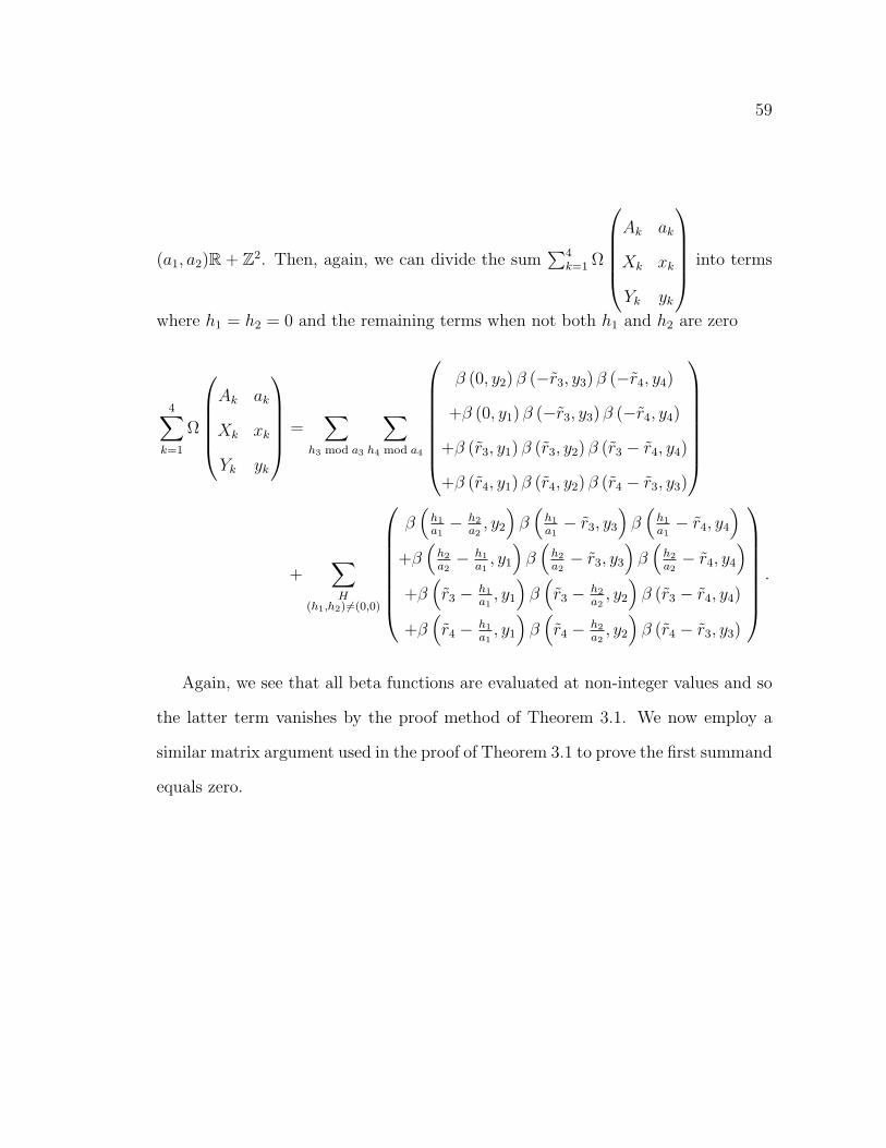
59
(a1, a2)R + Z2. Then, again, we can divide the sum∑4
k=1 Ω
Ak ak
Xk xk
Yk yk
into terms
where h1 = h2 = 0 and the remaining terms when not both h1 and h2 are zero
4∑k=1
Ω
Ak ak
Xk xk
Yk yk
=∑
h3 mod a3
∑h4 mod a4
β (0, y2) β (−r3, y3) β (−r4, y4)
+β (0, y1) β (−r3, y3) β (−r4, y4)
+β (r3, y1) β (r3, y2) β (r3 − r4, y4)
+β (r4, y1) β (r4, y2) β (r4 − r3, y3)
+∑H
(h1,h2) 6=(0,0)
β(
h1
a1− h2
a2, y2
)β
(h1
a1− r3, y3
)β
(h1
a1− r4, y4
)+β
(h2
a2− h1
a1, y1
)β
(h2
a2− r3, y3
)β
(h2
a2− r4, y4
)+β
(r3 − h1
a1, y1
)β
(r3 − h2
a2, y2
)β (r3 − r4, y4)
+β(r4 − h1
a1, y1
)β
(r4 − h2
a2, y2
)β (r4 − r3, y3)
.
Again, we see that all beta functions are evaluated at non-integer values and so
the latter term vanishes by the proof method of Theorem 3.1. We now employ a
similar matrix argument used in the proof of Theorem 3.1 to prove the first summand
equals zero.
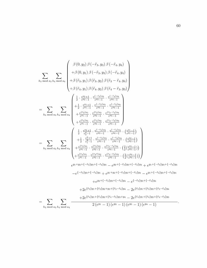
60
∑h3 mod a3
∑h4 mod a4
β (0, y2) β (−r3, y3) β (−r4, y4)
+β (0, y1) β (−r3, y3) β (−r4, y4)
+β (r3, y1) β (r3, y2) β (r3 − r4, y4)
+β (r4, y1) β (r4, y2) β (r4 − r3, y3)
=∑
h3 mod a3
∑h4 mod a4
12· ey2+1
ey2−1· e−r3y3
ey3−1· e−r4y4
ey4−1
+12· ey1+1
ey1−1· e−r3y3
ey3−1· e−r4y4
ey4−1
+ er3y1
ey1−1· er3y2
ey2−1· er3−r4y4
ey4−1
+ er4y1
ey1−1· er4y2
ey2−1· er4−r3y3
ey3−1
=∑
h3 mod a3
∑h4 mod a4
12· ey2+1
ey2−1
· e−r3y3
ey3−1· e−r4y4
ey4−1·(
ey1−1ey1−1
)+1
2· ey
1+1
ey1−1
· e−r3y3
ey3−1· e−r4y4
ey4−1·(
ey2−1ey2−1
)+ er3y1
ey1−1· er3y2
ey2−1· er3−r4y4
ey4−1·(
22( ey3−1
ey3−1))
+ er4y1
ey1−1· er4ry2
ey2−1· er4−r3y3
ey3−1·(
22( ey4−1
ey4−1))
=∑
h3 mod a3
∑h4 mod a4
ey1+y2+−r3y3+−r4y4 − ey2+−r3y3+−r4y4 + ey1+−r3y3+−r4y4
−e−r3y3+−r4y4 + ey1+y2+−r3y3+−r4y4 − ey1+−r3y3+−r4y4
+ey2+−r3y3+−r4y4 − e−r3y3+−r4y4
+2er3y1+r3y2+y3+r3−r4y4 − 2er3y1+r3y2+r3−r4y4
+2er4y1+r4y2+r4−r3y3+y4 − 2er4y1+r4y2+r4−r3y3
2 (ey1 − 1) (ey2 − 1) (ey3 − 1) (ey4 − 1).
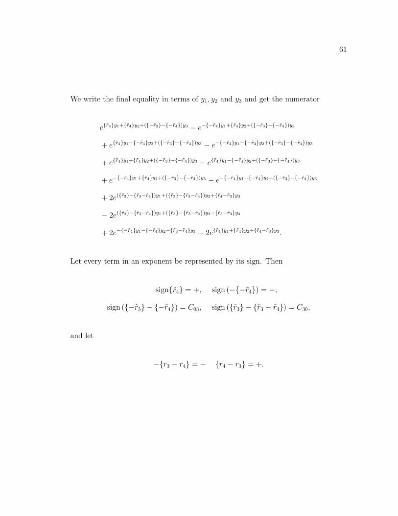
61
We write the final equality in terms of y1, y2 and y3 and get the numerator
er4y1+r4y2+(−r3−−r4)y3 − e−−r4y1+r4y2+(−r3−−r4)y3
+ er4y1−−r4y2+(−r3−−r4)y3 − e−−r4y1−−r4y2+(−r3−−r4)y3
+ er4y1+r4y2+(−r3−−r4)y3 − er4y1−−r4y2+(−r3−−r4)y3
+ e−−r4y1+r4y2+(−r3−−r4)y3 − e−−r4y1−−r4y2+(−r3−−r4)y3
+ 2e(r3−r3−r4)y1+(r3−r3−r4)y2+r4−r3y3
− 2e(r3−r3−r4)y1+(r3−r3−r4)y2−r3−r4y4
+ 2e−−r4y1−−r4y2−r3−r4y3 − 2er4y1+r4y2+r4−r3y3 .
Let every term in an exponent be represented by its sign. Then
signr4 = +, sign (−−r4) = −,
sign (−r3 − −r4) = C03, sign (r3 − r3 − r4) = C30,
and let
−r3 − r4 = − r4 − r3 = +.
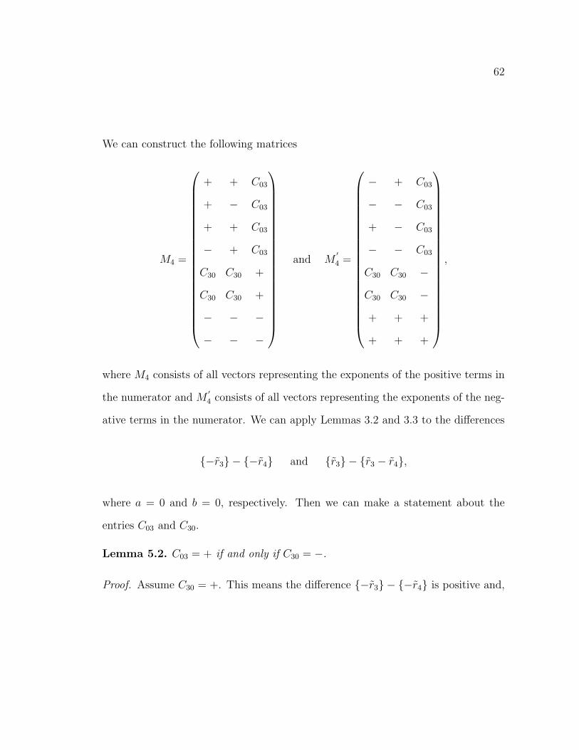
62
We can construct the following matrices
M4 =
+ + C03
+ − C03
+ + C03
− + C03
C30 C30 +
C30 C30 +
− − −
− − −
and M′
4 =
− + C03
− − C03
+ − C03
− − C03
C30 C30 −
C30 C30 −
+ + +
+ + +
,
where M4 consists of all vectors representing the exponents of the positive terms in
the numerator and M′4 consists of all vectors representing the exponents of the neg-
ative terms in the numerator. We can apply Lemmas 3.2 and 3.3 to the differences
−r3 − −r4 and r3 − r3 − r4,
where a = 0 and b = 0, respectively. Then we can make a statement about the
entries C03 and C30.
Lemma 5.2. C03 = + if and only if C30 = −.
Proof. Assume C30 = +. This means the difference −r3 − −r4 is positive and,
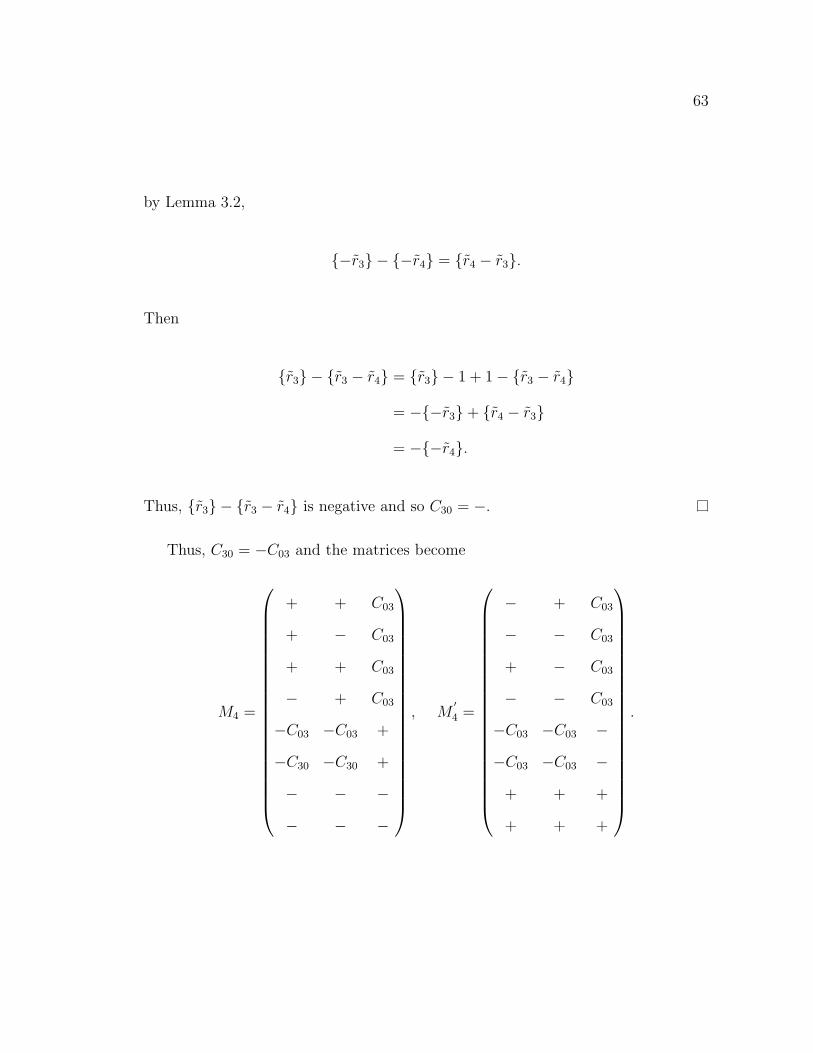
63
by Lemma 3.2,
−r3 − −r4 = r4 − r3.
Then
r3 − r3 − r4 = r3 − 1 + 1− r3 − r4
= −−r3+ r4 − r3
= −−r4.
Thus, r3 − r3 − r4 is negative and so C30 = −.
Thus, C30 = −C03 and the matrices become
M4 =
+ + C03
+ − C03
+ + C03
− + C03
−C03 −C03 +
−C30 −C30 +
− − −
− − −
, M′
4 =
− + C03
− − C03
+ − C03
− − C03
−C03 −C03 −
−C03 −C03 −
+ + +
+ + +
.
64
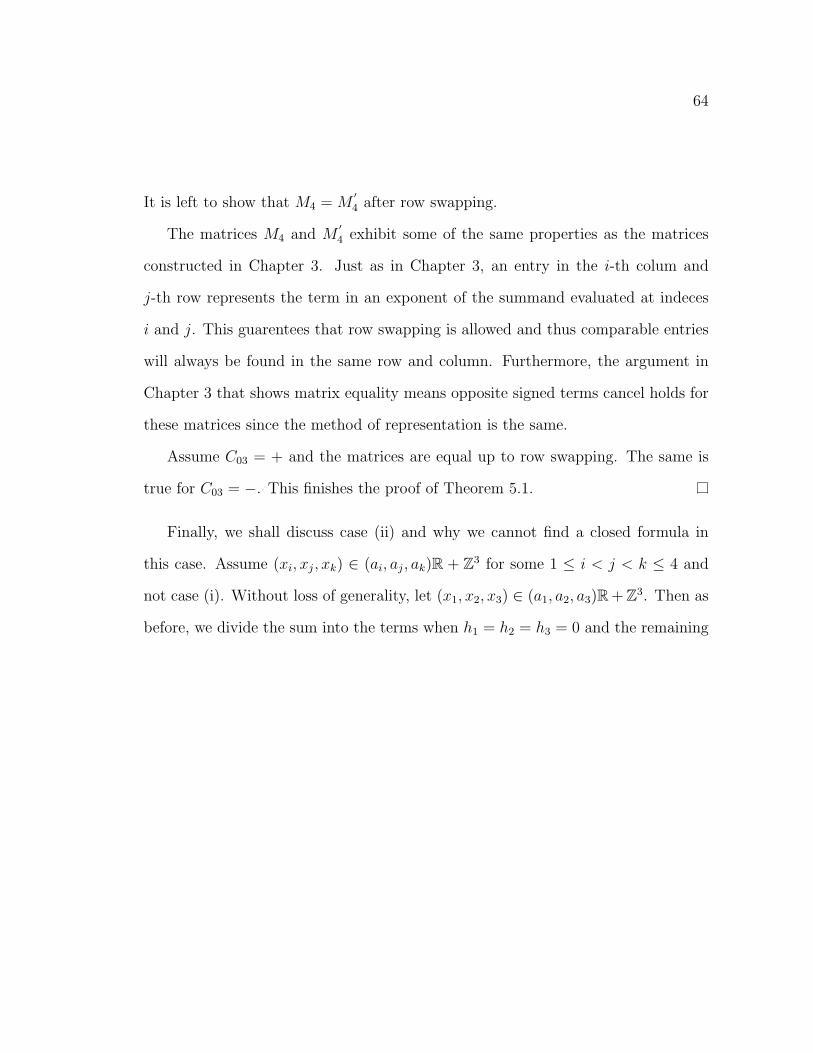
It is left to show that M4 = M′4 after row swapping.
The matrices M4 and M′4 exhibit some of the same properties as the matrices
constructed in Chapter 3. Just as in Chapter 3, an entry in the i-th colum and
j-th row represents the term in an exponent of the summand evaluated at indeces
i and j. This guarentees that row swapping is allowed and thus comparable entries
will always be found in the same row and column. Furthermore, the argument in
Chapter 3 that shows matrix equality means opposite signed terms cancel holds for
these matrices since the method of representation is the same.
Assume C03 = + and the matrices are equal up to row swapping. The same is
true for C03 = −. This finishes the proof of Theorem 5.1.
Finally, we shall discuss case (ii) and why we cannot find a closed formula in
this case. Assume (xi, xj, xk) ∈ (ai, aj, ak)R + Z3 for some 1 ≤ i < j < k ≤ 4 and
not case (i). Without loss of generality, let (x1, x2, x3) ∈ (a1, a2, a3)R + Z3. Then as
before, we divide the sum into the terms when h1 = h2 = h3 = 0 and the remaining
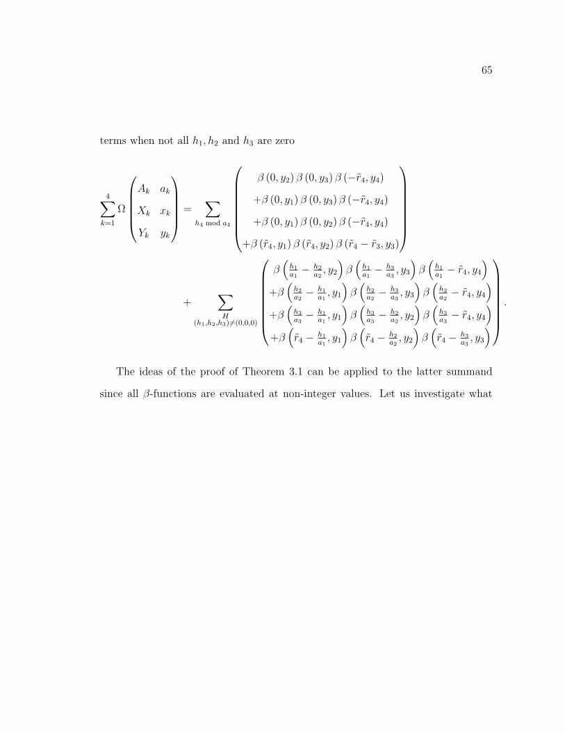
65
terms when not all h1, h2 and h3 are zero
4∑k=1
Ω
Ak ak
Xk xk
Yk yk
=∑
h4 mod a4
β (0, y2) β (0, y3) β (−r4, y4)
+β (0, y1) β (0, y3) β (−r4, y4)
+β (0, y1) β (0, y2) β (−r4, y4)
+β (r4, y1) β (r4, y2) β (r4 − r3, y3)
+∑H
(h1,h2,h3) 6=(0,0,0)
β(
h1
a1− h2
a2, y2
)β
(h1
a1− h3
a3, y3
)β
(h1
a1− r4, y4
)+β
(h2
a2− h1
a1, y1
)β
(h2
a2− h3
a3, y3
)β
(h2
a2− r4, y4
)+β
(h3
a3− h1
a1, y1
)β
(h3
a3− h2
a2, y2
)β
(h3
a3− r4, y4
)+β
(r4 − h1
a1, y1
)β
(r4 − h2
a2, y2
)β
(r4 − h3
a3, y3
)
.
The ideas of the proof of Theorem 3.1 can be applied to the latter summand
since all β-functions are evaluated at non-integer values. Let us investigate what
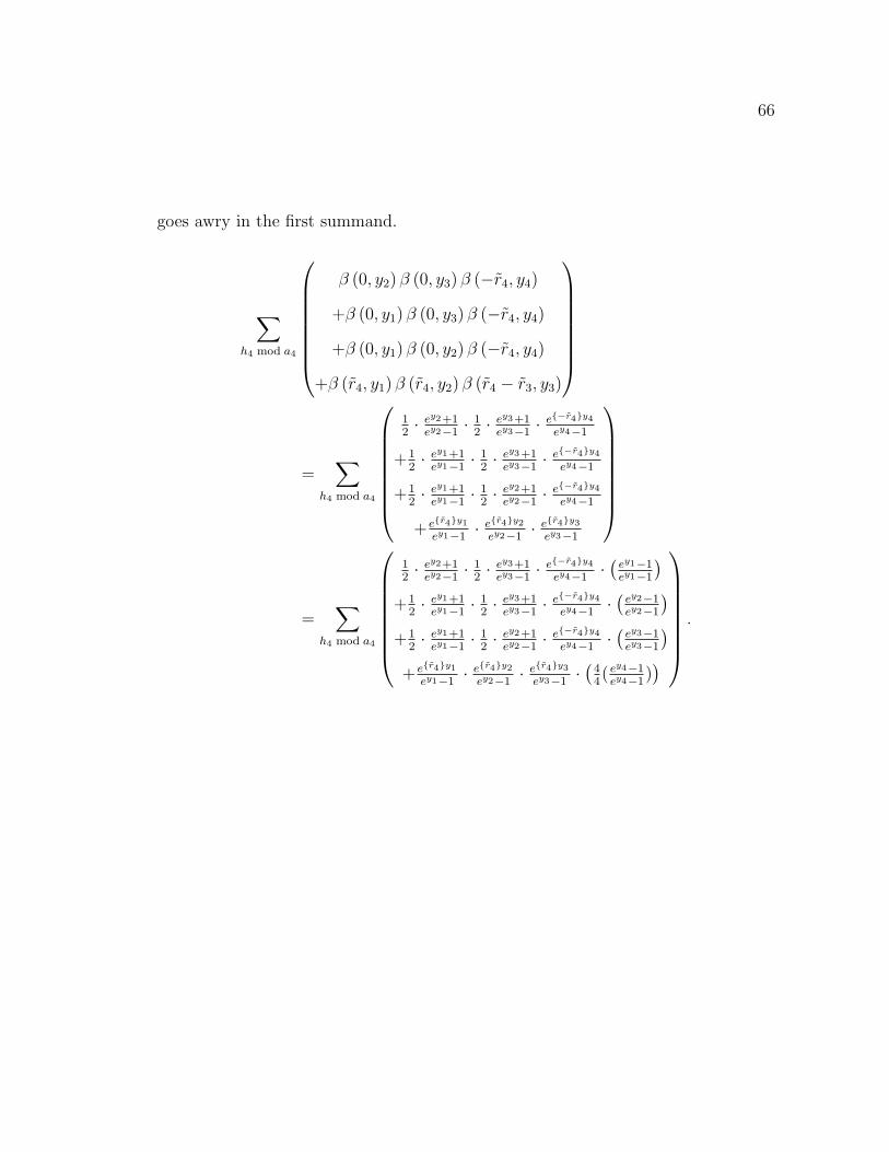
66
goes awry in the first summand.
∑h4 mod a4
β (0, y2) β (0, y3) β (−r4, y4)
+β (0, y1) β (0, y3) β (−r4, y4)
+β (0, y1) β (0, y2) β (−r4, y4)
+β (r4, y1) β (r4, y2) β (r4 − r3, y3)
=∑
h4 mod a4
12· ey2+1
ey2−1· 1
2· ey3+1
ey3−1· e−r4y4
ey4−1
+12· ey1+1
ey1−1· 1
2· ey3+1
ey3−1· e−r4y4
ey4−1
+12· ey1+1
ey1−1· 1
2· ey2+1
ey2−1· e−r4y4
ey4−1
+ er4y1
ey1−1· er4y2
ey2−1· er4y3
ey3−1
=∑
h4 mod a4
12· ey2+1
ey2−1· 1
2· ey3+1
ey3−1· e−r4y4
ey4−1·(
ey1−1ey1−1
)+1
2· ey1+1
ey1−1· 1
2· ey3+1
ey3−1· e−r4y4
ey4−1·(
ey2−1ey2−1
)+1
2· ey1+1
ey1−1· 1
2· ey2+1
ey2−1· e−r4y4
ey4−1·(
ey3−1ey3−1
)+ er4y1
ey1−1· er4y2
ey2−1· er4y3
ey3−1·(
44( ey4−1
ey4−1))
.
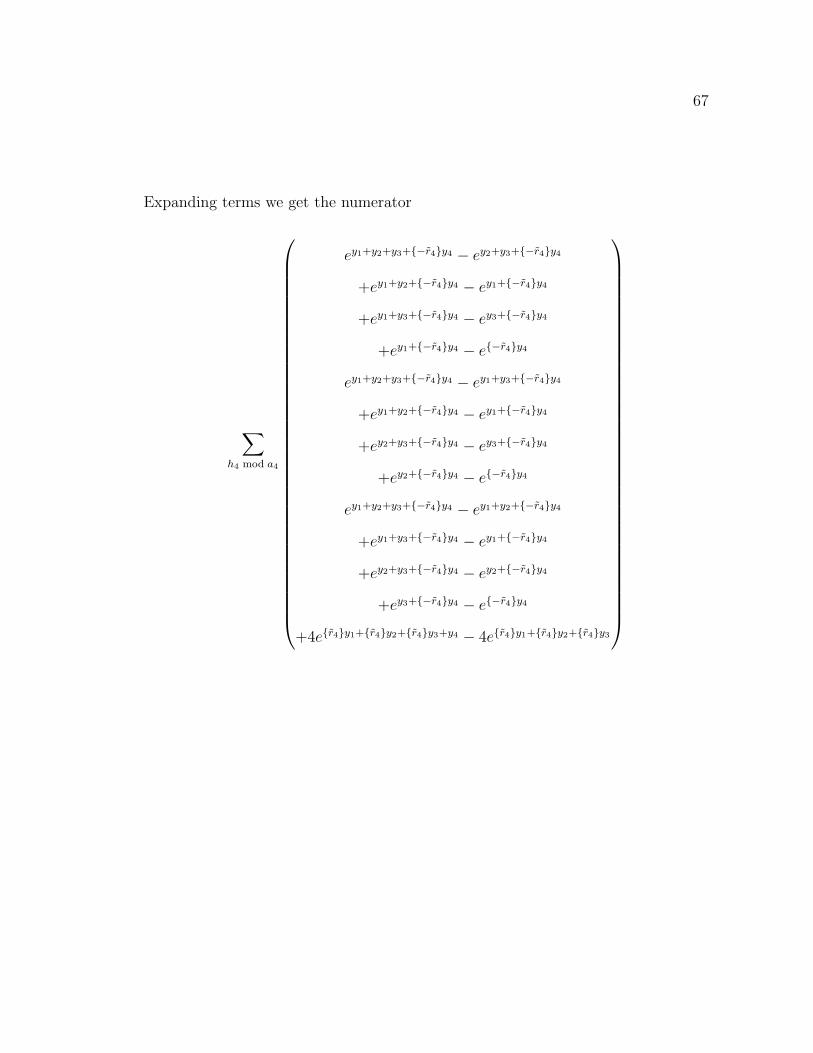
67
Expanding terms we get the numerator
∑h4 mod a4
ey1+y2+y3+−r4y4 − ey2+y3+−r4y4
+ey1+y2+−r4y4 − ey1+−r4y4
+ey1+y3+−r4y4 − ey3+−r4y4
+ey1+−r4y4 − e−r4y4
ey1+y2+y3+−r4y4 − ey1+y3+−r4y4
+ey1+y2+−r4y4 − ey1+−r4y4
+ey2+y3+−r4y4 − ey3+−r4y4
+ey2+−r4y4 − e−r4y4
ey1+y2+y3+−r4y4 − ey1+y2+−r4y4
+ey1+y3+−r4y4 − ey1+−r4y4
+ey2+y3+−r4y4 − ey2+−r4y4
+ey3+−r4y4 − e−r4y4
+4er4y1+r4y2+r4y3+y4 − 4er4y1+r4y2+r4y3
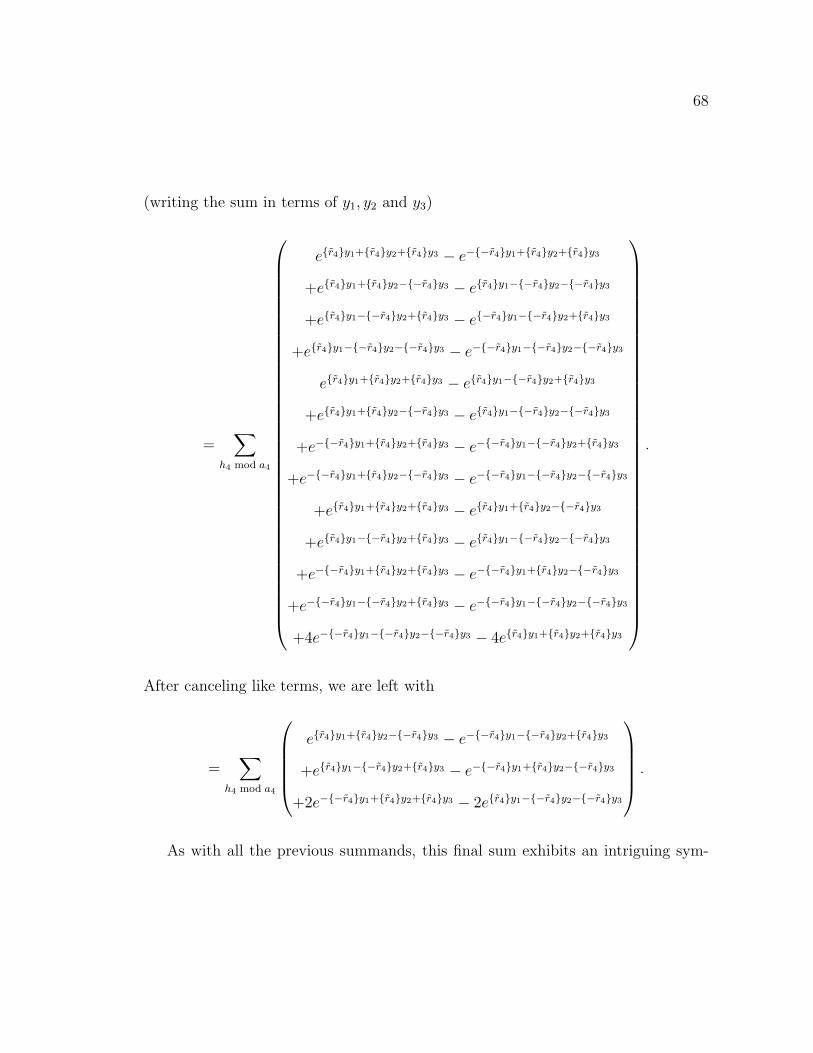
68
(writing the sum in terms of y1, y2 and y3)
=∑
h4 mod a4
er4y1+r4y2+r4y3 − e−−r4y1+r4y2+r4y3
+er4y1+r4y2−−r4y3 − er4y1−−r4y2−−r4y3
+er4y1−−r4y2+r4y3 − e−r4y1−−r4y2+r4y3
+er4y1−−r4y2−−r4y3 − e−−r4y1−−r4y2−−r4y3
er4y1+r4y2+r4y3 − er4y1−−r4y2+r4y3
+er4y1+r4y2−−r4y3 − er4y1−−r4y2−−r4y3
+e−−r4y1+r4y2+r4y3 − e−−r4y1−−r4y2+r4y3
+e−−r4y1+r4y2−−r4y3 − e−−r4y1−−r4y2−−r4y3
+er4y1+r4y2+r4y3 − er4y1+r4y2−−r4y3
+er4y1−−r4y2+r4y3 − er4y1−−r4y2−−r4y3
+e−−r4y1+r4y2+r4y3 − e−−r4y1+r4y2−−r4y3
+e−−r4y1−−r4y2+r4y3 − e−−r4y1−−r4y2−−r4y3
+4e−−r4y1−−r4y2−−r4y3 − 4er4y1+r4y2+r4y3
.
After canceling like terms, we are left with
=∑
h4 mod a4
er4y1+r4y2−−r4y3 − e−−r4y1−−r4y2+r4y3
+er4y1−−r4y2+r4y3 − e−−r4y1+r4y2−−r4y3
+2e−−r4y1+r4y2+r4y3 − 2er4y1−−r4y2−−r4y3
.
As with all the previous summands, this final sum exhibits an intriguing sym-
69
metry among the exponents. And though it is not yet clear how, it is quite possible
that these few terms combine to equal something simple. The unknown fate of
this extraneous case gives light to the level of complexity that builds when dealing
with higher dimensional Dedekind–Bernoulli sums. Although our work and Bayad
and Raouj’s work shows the extreme cases of Hall, Wilson and Zagier’s reciprocity
law can be generalized, the 4-variable reciprocity Theorem shows us the more vari-
ables involved the more challenging computations become and generalizations of the
intermediate cases are not strait forward. We leave this open question to the reader.
Bibliography
[1] T. M. Apostol, Generalized Dedekind sums and transformation formulae ofcertain Lambert series, Duke Math. J. 17 (1950), 147–157.
[2] Tom M. Apostol, Introduction to analytic number theory, Springer-Verlag, NewYork, 1976.
[3] Abdelmejid Bayad and Abdelaziz Raouj, Reciprocity formulae for general mul-tiple Dedekind–Rademacher sums and enumerations of lattice points, preprint(2009).
[4] Matthias Beck and Sinai Robins, Computing the continuous discretely, Under-graduate Texts in Mathematics, Springer, New York, 2007.
[5] L. Carlitz, Some theorems on generalized Dedekind sums, Pacific J. Math. 3(1953), 513–522.
[6] Ulrich Dieter, Beziehungen zwischen Dedekindschen Summen, Abh. Math. Sem.Univ. Hamburg 21 (1957), 109–125.
[7] R. R. Hall, J. C. Wilson, and D. Zagier, Reciprocity formulae for generalDedekind-Rademacher sums, Acta Arith. 73 (1995), no. 4, 389–396.
[8] Donald E. Knuth, The art of computer programming. Vol. 2, second ed.,Addison-Wesley Publishing Co., Reading, Mass., 1981.
[9] W. Meyer and R. Sczech, Uber eine topologische und zahlentheoretische Anwen-dung von Hirzebruchs Spitzenauflosung, Math. Ann. 240 (1979), no. 1, 69–96.
70
71
[10] M. Mikolas, On certain sums generating the Dedekind sums and their reciprocitylaws, Pacific J. Math. 7 (1957), 1167–1178.
[11] Hans Rademacher, Generalization of the reciprocity formula for Dedekind sums,Duke Math. J. 21 (1954), 391–397.
[12] Hans Rademacher and Emil Grosswald, Dedekind sums, The MathematicalAssociation of America, Washington, D.C., 1972.
[13] Hans Rademacher and Albert Whiteman, Theorems on Dedekind sums, Amer.J. Math. 63 (1941), 377–407.