Embed Size (px)
Citation preview
DEPARTMENT OF MATHEMATICSTECHNICAL REPORT
Generalized Cross-Validation for Correlated Data (GCVc)
Patrick S. Carmack
March 2011
No. 2011 – 1
UNIVERSITY OF CENTRAL ARKANSASConway, AR 72035

GENERALIZED CROSS-VALIDATION FOR CORRELATED DATA
(GCVc)
PATRICK S. CARMACK†
Department of MathematicsUniversity of Central Arkansas
201 Donaghey Avenue, Conway, AR 72035-5001, USA
JEFFREY S. SPENCE
Department of Internal Medicine, Epidemiology DivisionUniversity of Texas Southwestern Medical Center at Dallas5323 Harry Hines Boulevard, Dallas, TX 75390-8874, USA
WILLIAM R. SCHUCANY
Department of Statistical ScienceSouthern Methodist University
P.O. Box 750332, Dallas, TX 75275-0332, USA
Abstract. Since its introduction by Stone (1974) and Geisser (1975), cross-validation
has been studied and improved by several authors including Burman et al. (1994), Hart
& Yi (1998), Racine (2000), Hart & Lee (2005), and Carmack et al. (2009). Perhaps
the most widely used and best known is generalized cross-validation (GCV) (Craven &
Wahba, 1979), which establishes a single-pass method that penalizes the fit by the trace
of the smoother matrix assuming independent errors. We propose an extension to GCV
in the context of correlated errors that has important implications about the definition
for residual degrees of freedom, even in the independent case. The efficacy of the new
method is demonstrated by simulation and application with concluding remarks about
the heteroscedastic case and a potential maximum likelihood framework.
E-mail addresses: [email protected], [email protected], [email protected]: March 28, 2011.
Key words and phrases. correlation, effective degrees of freedom, linear smoother, model selection.†Corresponding author.
1

2
1. Introduction
Cross-validation has a rich history starting with ordinary cross-validation (Stone, 1974;Geisser, 1975). The original method works by withholding a single data point at a timewhile using the rest of the data to predict the withheld response. In the context of modelselection, the model with the smallest cross-validated squared error is then declared to bethe best one. Ordinary cross-validation is not consistent for model selection, but v-foldcross-validation addresses this issue by randomly partitioning the data into training andtest sets where models are fit using training sets and assessed using test sets. Both of thesemethods assume independent errors.
Subsequent papers extended cross-validation for correlated data. One known as h-blockcross-validation (Burman et al., 1994) did so by withholding blocks of data when estimatingparameters and using the full dataset for model assessment. Racine (2000) combined h-block and v-fold cross-validation to arrive at a consistent method, hv-block cross-validation.Hart & Yi (1998) proposed one-sided cross-validation, which omits the data either to theleft or right of the point of estimation, including the point, and then assesses squarederror performance. While initially intended for independent errors, Hart & Lee (2005)demonstrated that the method is robust in the presence of low to moderately correlatederrors. Finally, Carmack et al. (2009) proposed a method similar to h-block cross-validationknown as far casting cross-validation (FCCV). Their method uses the full dataset to esti-mate model parameters while omitting certain neighbors for model assessment purposes.
Craven & Wahba (1979) proposed a single-pass consistent method for independent dataknown as generalized cross-validation (GCV). Their ingenious use of degrees of freedommakes this possible and is a concept that we extend to correlated data. We motivate theextension, generalized cross-validation for correlated data (GCVc), from a nonparametricperspective, but conclude with some interesting connections to a parametric setting.
2. Theory
Suppose yi = f(xi) + εi, i = 1, . . . , n, where f(·) is a function, and εi is stochastic withE[εi] = 0, Var[εi] = σ2 < ∞, and n × n covariance matrix given by (Σ)ij = σ2(C)ij =
σ2cor(εi, εj) = σ2rij , C = J . We are interested in finding f(·) to estimate f(·), which we
assume takes the form of a linear smoother. That is, f(x) =n
i=1wiyi, where the weights,w1, . . . , wn, are a function of x and a vector of tuning parameters, θ, with
ni=1wi = 1.
Many cross-validation techniques are commonly used to estimate such tuning parametersby
θ = argminθ
CV(θ) =1
n
n
k=1
fcv (xk | θ)− yk
2,
GENERALIZED CROSS-VALIDATION FOR CORRELATED DATA (GCVc) 3
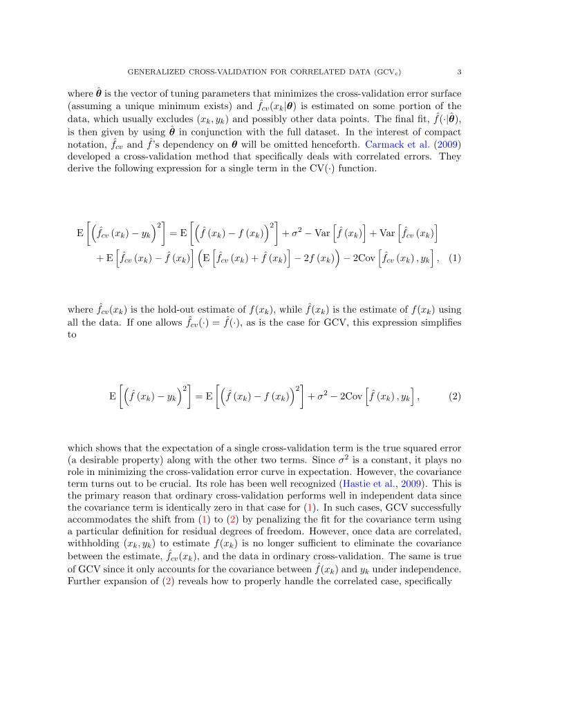
where θ is the vector of tuning parameters that minimizes the cross-validation error surface(assuming a unique minimum exists) and fcv(xk|θ) is estimated on some portion of thedata, which usually excludes (xk, yk) and possibly other data points. The final fit, f(·|θ),is then given by using θ in conjunction with the full dataset. In the interest of compactnotation, fcv and f ’s dependency on θ will be omitted henceforth. Carmack et al. (2009)developed a cross-validation method that specifically deals with correlated errors. Theyderive the following expression for a single term in the CV(·) function.
E
fcv (xk)− yk
2= E
f (xk)− f (xk)
2+ σ2 −Var
f (xk)
+Var
fcv (xk)
+ Efcv (xk)− f (xk)
Efcv (xk) + f (xk)
− 2f (xk)
− 2Cov
fcv (xk) , yk
, (1)
where fcv(xk) is the hold-out estimate of f(xk), while f(xk) is the estimate of f(xk) usingall the data. If one allows fcv(·) = f(·), as is the case for GCV, this expression simplifiesto
E
f (xk)− yk
2= E
f (xk)− f (xk)
2+ σ2 − 2Cov
f (xk) , yk
, (2)
which shows that the expectation of a single cross-validation term is the true squared error(a desirable property) along with the other two terms. Since σ2 is a constant, it plays norole in minimizing the cross-validation error curve in expectation. However, the covarianceterm turns out to be crucial. Its role has been well recognized (Hastie et al., 2009). This isthe primary reason that ordinary cross-validation performs well in independent data sincethe covariance term is identically zero in that case for (1). In such cases, GCV successfullyaccommodates the shift from (1) to (2) by penalizing the fit for the covariance term usinga particular definition for residual degrees of freedom. However, once data are correlated,withholding (xk, yk) to estimate f(xk) is no longer sufficient to eliminate the covariancebetween the estimate, fcv(xk), and the data in ordinary cross-validation. The same is trueof GCV since it only accounts for the covariance between f(xk) and yk under independence.Further expansion of (2) reveals how to properly handle the correlated case, specifically

4 P. CARMACK, J. SPENCE, AND W. SCHUCANY
E
f (xk)− yk
2= E
f (xk)− f (xk)
2+ σ2 − 2Cov
f (xk) , yk
=
n
i=1
wif (xi)− f (xk)
2
+Varf (xk)
+ σ2 − 2Cov
f (xk) , yk
=
n
i=1
wif (xi)− f (xk)
2
+ σ2 +n
i=1
n
j=1
wiwjσij − 2n
i=1
wiσik
=
n
i=1
wif (xi)− f (xk)
2
+ σ2
1 +n
i=1
n
j=1
wiwjrij − 2n
i=1
wirik
.
Letting f(x) = Sy, where (S)ij = wij , µk =n
i=1wkiyi − yk, and Rk = rk +ni=1
nj=1wkiwjrij −
ni=1wkiri −
ni=1wirki, one can now show that
E
n
k=1
f (xk)− yk
2=
n
k=1
µ2k + σ2
n
k=1
Rkk
=n
k=1
µ2k + σ2tr
C + SCS − 2SC
.
Provided that C = I and the smoother matrix S is symmetric and idempotent, as isthe case for many linear fitting techniques, the trace term reduces to n − tr[S], which isproportional to the familiar denominator in GCV.
Historically, there are three major contenders for defining residual degrees of freedomunder independence in the context of linear smoothers (Buja et al., 1989). These are allequivalent for S idempotent and symmetric, namely
trI −
2S − SS , (3)
tr [I − S] , and (4)
trI − SS . (5)
In light of the preceding discussion, we propose the following definition for residualdegrees of freedom:
trC + SCS − 2SC
= n− tr
2SC − SCS , (6)

GENERALIZED CROSS-VALIDATION FOR CORRELATED DATA (GCVc) 5
which is the analogue of (3) when taking correlation into account. As shown by Buja et al.(1989) through eigen decomposition, tr[I − (2S − SS)] ≤ tr[I − S] ≤ tr[I − SS]. Thisimplies that (6) is the most stringent of the three and differs from (4) employed by GCVeven in the independent case. Adopting this definition of degrees of freedom leads us todefine the generalized cross-validation for correlated data surface as
GCV(1)c (θ) =
1
n
nk=1 yk − f (xk)
1− tr [2SC − SCS] /n
2
, (7)
with θ as its minimizer provided 0 S ≺ I.
3. Simulations
The simulation study here is similar to that of Carmack et al. (2009), where FCCV wasshown to perform as well as or better than other cross-validation methods in correlateddata. We are interested in assessing the performance of the included methods whose task isto select a global bandwidth for local linear regression (Fan, 1992) with serially correlatedadditive errors. The local linear regression estimate is given by
f (xk | h) =n
i=1wi (xi | h) yini=1wi (xi | h)
, where
wi (x | h) = K
x− xi
h
(tn,2 − (x− xi) tn,1) , and
tn,j (x | h) =n
i=1
K
x− xi
h
(x− xi)
j , j = 1, 2.
The tricube kernel, K(u) = 35/32(1− u2)3, 0 ≤ u ≤ 1, was chosen for our purposes. Thefollowing four functions were selected for variety of structure (Fig. 1):
f1 (x) = x3 (1− x)3 ,
f2 (x) = (x/2)3 (1− x/2)2 ,
f3 (x) = 1.741 ·2x10 (1− x)2 + x2 (1− x)10
, and
f4 (x) =
0.0212 · exp (x− 1/3) , x < 1/30.0212 · exp (−2 (x− 1/3))) , x ≥ 1/3
.
Each function, f(·) = f1(·), f2(·), f3(·), or f4(·), was sampled at either n = 75 or n = 150equally spaced design points in the interval [0, 1] with xi = (i − 0.5)/n, i = 1, . . . , n. Avector of serially correlated errors, εi, i = 1, . . . , n, was generated using arima.sim in R

6 P. CARMACK, J. SPENCE, AND W. SCHUCANY
(R Development Core Team, 2010) from a first-order autoregressive process (AR(1)) withcoefficient φ = 0.0, 0.3, 0.6, or 0.9, which ranges from independent to heavily correlated,and standard deviation σ = 2−11, 2−9, or 2−7, which ranges from low to high variance.Each realization results in a dataset (xi, f(xi)+ εi), i = 1, . . . , n, which was repeated 1,000times for each combination of f(·), n, φ, and σ.
For comparison, we included FCCV along with the following:
GCV(2)c (θ) =
1
n
nk=1 yk − f (xk)
1− tr [SC] /n
2
, and (8)
GCV(3)c (θ) =
1
n
nk=1 yk − f (xk)
1− tr [SCS] /n
2
, (9)
whose denominators are proportional to the correlated analogues of (4) and (5), respec-tively.
For each realization, one bandwidth was estimated as the minimizer of (7), (8), (9), orthe FCCV error curve with the withholding neighborhood d set to the recommended valueof 3/n. The function optimize in R was used for all four methods with 0 ≤ h ≤ 1. For thethree GCVc criteria, the correlation matrix C was either assumed known or estimated usingthe first five lags of the raw empirical semivariogram of the data fit using a nonparametricsemivariogram estimator. The raw empirical semivariogram for a time series at lag k is γk =
|i−j|=k(yi−yj)2/2(n−k) with the nonparametric fit given by γ(k) =m
i=1[1−Ωκ(kti)]pi,where κ is the order of the basis set to 11 for our purposes, and pi, i = 1, . . . ,m, is thenonnegative least squares minimizer of
5k=1(γk − γ(k))2. See Cherry et al. (1996) for
further details concerning the nonparametric semivariogram estimator. One should notethat γk is a biased estimate of the semivariance at lag k since the data contains meanstructure (i.e., E[γk] = σ2(1 − φk)/(1 − φ2) +
|i−j|=k[f(xi) − f(xj)]2/[2(n − k)]), which
is why the nonparametric semivariogram is fit using the first five lags of the empiricalsemivariogram where differencing hopefully removes much of the mean structure at lagsclose together. The nonparametric semivariogram is then used to estimate C as
C
ij= 1− γ (|i− j|)m
i=1 pi,
wherem
i=1 pi is the sill estimate, which represents the variance of observations far apart.
Once each of the four methods yielded an estimate of bandwidth, h, for each iteration,the average squared error was calculated as

GENERALIZED CROSS-VALIDATION FOR CORRELATED DATA (GCVc) 7
ASEh=
1
n
n
i=1
f (xi)− f
xi | h
2,
which will be our basis for comparison. Additionally, the bandwidth, h0, for each iterationand associated ASE, ASE0, using full knowledge of the underlying function was estimatedto serve as a baseline.
As Figs. 3 and 4 (reviewers please see Figs. 7–12 in the Appendix) demonstrate, GCV(1)c
dominates both GCV(2)c and GCV(3)
c provided the correlation structure is known in termsof mean ASE ratio. This is not the case when the correlation structure is estimated whereGCV(1)
c exhibits considerably higher mean ASE ratios when the error variance is low. An
inspection of the bandwidth estimates showed that GCV(1)c tends to over smooth in these
cases. Table 1 (reviewers please see Tables 2–4) contains the means of the ratios of eachmethods estimated bandwidth and h0 for each iteration. Further investigation revealedthat the bias in the empirical semivariogram is the cause since the magnitude of the func-tion overwhelms that of the variance in the bias expression given above. This phenomenon
causes the correlation to be overestimated, which GCV(1)c punishes more heavily than ei-
ther GCV(2)c or GCV(3)
c , especially at lower bandwidths (Fig. 5). However, GCV(1)c again
dominates the other two at medium and high variances when estimating C. Although theresults for f2(·), f3(·), and f4(·) are not shown, the preceding comments generally apply tothem as well.
Further study of Table 1 (reviewers please see Tables 2–4) shows that GCV(2)c appears to
be less biased for h0 than GCV(1)c when the correlation structure is known with the latter
selecting higher bandwidths on average. However, GCV(2)c ’s reduced bias for h0 appears to
come at the price of higher average ASE relative to that of GCV(1)c . This is likely a case of
bias-variance tradeoff since GCV(1)c accounts for the total variance of C+SCS−SC−CS
when the errors are multivariate normal as the discussion section shows.
FCCV performed well, often besting GCV(2)c and GCV(3)
c in terms of mean ASE. The
same is true of GCV(1)c when the variance is low and C is estimated. This is somewhat
surprising given FCCV’s simplistic approach of omitting neighborhoods about the point ofestimation. In cases where the correlation structure proves difficult to estimate, FCCV isan excellent alternative to GCVc.
4. Application
Although the covariance matrix for an empirical semivariogram is heteroscedastic, thereis an intimate relationship between the covariance structure of the semivariogram and the

8 P. CARMACK, J. SPENCE, AND W. SCHUCANY
semivariogram itself that can be accommodated by our proposed method. Parametricsemivariograms are frequently fit using weighted least squares (Cressie, 1985) by
θ = argminθ
i=1
Nsi
γ (si | θ)2(γ (si)− γ (si | θ))2
= argminθ
i=1
Nsi
γ (si)
γ (si | θ)− 1
2
, (10)
since Var[γ(s)] ≈ 2(γ(s))2/Ns, where γ(·) is the true semivariogram, γ(·) is the empiricalsemivariogram calculated from data, γ(·|θ) is a parametric semivariogram fit, Ns is thenumber of spatial locations s units apart, and is the number of lags used in the fittingprocess. Since each empirical semivariogram value has been divided by an estimate of itsstandard deviation, the covariance matrix of the ratios can now be treated as a correlationmatrix. Furthermore, the semivariogram provides an estimate of the covariance of the dataused to calculate the empirical semivariogram, which allows us to estimate the correlationmatrix of the ratios γ(si)/γ(si|θ), i = 1, . . . , (Genton, 1998).
In the application that follows, we fit a semiparametric semivariogram based on themethod presented by Carmack et al. (2011) replacing their fitting criterion using a modi-fied version of (10).
θ = argminθ
i=1
Nsi
γ(si)
γ(si|θ) − 1
1− tr2S C − S CS
/
2
, (11)
where C is the estimated correlation matrix of γ(si)/γ(si|θ), i = 1, . . . , , using a pilotestimate for γ(·|θ), and θ = [κ,α]. κ is the order of the basis with lower orders beingmore flexible, while α controls how the basis approaches the origin, which has an impor-tant impact on nugget estimation. The pilot fit used κ = 11, and α = 1. In their paper,Carmack et al. (2011) estimated α using a custom fitting criterion, but fixed κ = 11 due todifficulties with establishing an objective function that could satisfactorily accommodate κand α simultaneously, which is likely due to the strong correlation inherent in the empiricalsemivariogram.
Our primary interest is analyzing brain imaging data where we routinely use spatialmodeling (kriging) for statistical inference (Spence et al., 2007). The particular examplehere deals with functional magnetic resonance imaging (fMRI) where a subject is placed ina magnet to perform an experiment. The magnet records changes in blood oxygen level de-pendent (BOLD) signals at thousands of locations across the brain with three dimensionalvolumes captured every few seconds. The temporal aspect of the data is usually removed

GENERALIZED CROSS-VALIDATION FOR CORRELATED DATA (GCVc) 9
through a variety of statistical modeling methods (Lindquist, 2008) where practioners arecommonly interested in estimating the hemodynamic response function (HRF) to identifylocations associated with the experimental protocol or in extracting features of the HRFat active locations.
The experiment in the example had the subject silently repeat nonsense words displayedon a monitor above their head for a total of 152 scans spaced 2 sec. apart. We then es-timated a 13 parameter finite impulse response function (FIR) under a linear convolutioninvariance assumption with the parameters spaced 2 sec. apart to match the temporalresolution of the scans and the maximum duration of the HRF after a stimulus is ap-plied (26 sec.). This was done at 1,557 spatial locations that comprise the left superiortemporal gyrus, a portion of the brain thought to be associated with the protocol. For ahealthy subject, the peak in the HRF generally occurs approximately 6 sec. after a stimu-lus. Hence, we will concern ourselves with the third FIR parameter at these 1,557 locations.
As Fig. 6 shows, the empirical semivariogram of the third FIR parameter exhibits spa-tial correlation to approximately 9 mm. Casual inspection of the empirical semivariogramsuggests a linear approach to the origin is reasonable with the exponential or sphericalparametric models being natural choices given their linear behavior towards the origin.A semiparametric fit was estimated using (11) in optim in R with boundary conditions3 ≤ κ ≤ 25, and 0 ≤ α ≤ 1. The lower bound on κ is necessary since this is a threedimensional spatial process, while the upper limit was set at 25 since the basis does notsubstantially change beyond that value. The bounds on α are established in Carmack et al.(2011). The optimization yielded κ = 20.6 and α = 0.709 with the resulting semiparamet-ric fit along with the parametric exponential and spherical fits shown in Fig. 6. The nuggetestimate, which plays a critical role in kriging, is 15% of the estimated sill compared to thenugget estimated at 9% of the estimated sill in Carmack et al. (2011). The exponentialand spherical fits produced nugget estimates of 0% and 20% of their respective estimatedsills. The exponential is clearly a poor fit overshooting the early lags and failing to levelout at later lags. While the spherical arguably does better at the early lags, it appears tooverestimate the range.
5. Discussion
As the theory section established, a natural definition for residual degrees of freedom istr[C + SCS − 2SC], which suggests an extension of GCV for correlated data as defined
by GCV(1)c . Historical consideration of three competing definitions for residual degrees of
freedom and their correlated counterparts led us to define GCV(2)c and GCV(3)
c . As the
simulation study showed, when the correlation structure is known, GCV(1)c tends to domi-
nate the other two. However, this is not universally the case when estimating correlation.
When the variance is low, GCV(1)c can lead to over smoothing since the bias due to the
underlying function in the empirical semivariogram becomes large relative to the variance,
10 P. CARMACK, J. SPENCE, AND W. SCHUCANY
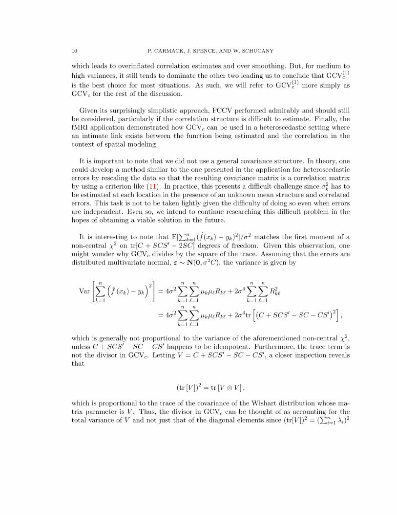
which leads to overinflated correlation estimates and over smoothing. But, for medium to
high variances, it still tends to dominate the other two leading us to conclude that GCV(1)c
is the best choice for most situations. As such, we will refer to GCV(1)c more simply as
GCVc for the rest of the discussion.
Given its surprisingly simplistic approach, FCCV performed admirably and should stillbe considered, particularly if the correlation structure is difficult to estimate. Finally, thefMRI application demonstrated how GCVc can be used in a heteroscedastic setting wherean intimate link exists between the function being estimated and the correlation in thecontext of spatial modeling.
It is important to note that we did not use a general covariance structure. In theory, onecould develop a method similar to the one presented in the application for heteroscedasticerrors by rescaling the data so that the resulting covariance matrix is a correlation matrixby using a criterion like (11). In practice, this presents a difficult challenge since σ2
k has tobe estimated at each location in the presence of an unknown mean structure and correlatederrors. This task is not to be taken lightly given the difficulty of doing so even when errorsare independent. Even so, we intend to continue researching this difficult problem in thehopes of obtaining a viable solution in the future.
It is interesting to note that E[n
k=1(f(xk) − yk)2]/σ2 matches the first moment of anon-central χ2 on tr[C + SCS − 2SC] degrees of freedom. Given this observation, onemight wonder why GCVc divides by the square of the trace. Assuming that the errors aredistributed multivariate normal, ε ∼ N(0,σ2C), the variance is given by
Var
n
k=1
f (xk)− yk
2= 4σ2
n
k=1
n
=1
µkµRk + 2σ4n
k=1
n
=1
R2k
= 4σ2n
k=1
n
=1
µkµRk + 2σ4trC + SCS − SC − CS2
,
which is generally not proportional to the variance of the aforementioned non-central χ2,unless C + SCS − SC − CS happens to be idempotent. Furthermore, the trace term isnot the divisor in GCVc. Letting V = C + SCS − SC − CS, a closer inspection revealsthat
(tr [V ])2 = tr [V ⊗ V ] ,
which is proportional to the trace of the covariance of the Wishart distribution whose ma-trix parameter is V . Thus, the divisor in GCVc can be thought of as accounting for thetotal variance of V and not just that of the diagonal elements since (tr[V ])2 = (
ni=1 λi)2

GENERALIZED CROSS-VALIDATION FOR CORRELATED DATA (GCVc) 11
and tr[V 2] =n
i=1 λ2i , where λi, i = 1, . . . , n, are the eigenvalues of V .
Continuing with normality, the characteristic function ofn
k=1(f(xk) − yk)2 when allthe non-centrality parameters are zero is given by (Krishnaiah, 1961)
ψ (t) = Πnj=1
1− it2σ2λj
− 12 .
This is a convolution of gammas with common shape parameter α = −1/2 and scaleparameters βj = 2σ2λj , j = 1, . . . , n, which is a kind of generalization of the χ2. Sev-eral methods exist for computing the distribution of convolutions of gammas with trun-cated series or Monte Carlo methods, but a more simplistic approach in the spirit of Sat-terthwaite is an approximation by a single gamma with α = (
nj=1 λj)2/(2
nj=1 λ
2j ) and
β = 2σ2nj=1 λ
2j/
nj=1 λj (Stewart et al., 2007), which we found to work well with low to
moderately correlated data with adequate sample sizes. In this framework, our proposedcross-validation criterion could be treated as estimating θ via maximum likelihood. Weopted not to present this approach at this time since we are striving to keep the presentmethod as nonparametric as possible, but this remains a promising avenue of research thatintend to pursue.
References
Buja, A., Hastie, T., & Tibsirani, R. (1989). Linear smoothers and additive models. TheAnnals of Statistics, 17 (2), 453–510.
Burman, P., Chow, E., & Nolan, D. (1994). A cross-validatory method for dependent data.Biometrika, 81 (2), 351–358.
Carmack, P., Spence, J., Schucany, W., Gunst, R., Lin, Q., & Haley, R. (2009). Far castingcross validation. Journal of Computational and Graphical Statistics, 18 (4), 879–893.
Carmack, P., Spence, J., Schucany, W., Gunst, R., Lin, Q., & Haley, R. (2011). A newclass of semiparametric semivariogram and nugget estimators. Computational Statisticsand Data Analysis, ? (?), ?–?
Cherry, S., Banfield, J., & Quimby, W. (1996). An evaluation of a nonparametric methodof estimating semivariograms of isotropic spatial processes. Journal of Applied Statistics,23 (4), 435–449.
Craven, P. & Wahba, G. (1979). Smoothing noisy data with spline functions. NumericalMathematics, 31, 377–403.
Cressie, N. (1985). Fitting variogram models by weighted least squares. MathematicalGeology, 17 (5), 563–586.
Fan, J. (1992). Design-adaptive nonparametric regression. Journal of the American Sta-tistical Association, 87, 998–1004.
Geisser, S. (1975). A predictive sample reuse method with applications. Journal of theAmerican Statistical Association, 70, 320–328.

12 P. CARMACK, J. SPENCE, AND W. SCHUCANY
Genton, M. (1998). Variogram fitting by generalized least squares using an explicit formulafor the covariance structure. Matematical Geology, 30 (4), 323–345.
Hart, J. & Lee, C. (2005). Robustness of one-sided cross-validation to autocorrelation.Journal of Multivariate Analysis, 92 (1), 77–96.
Hart, J. & Yi, S. (1998). One-sided cross-validation. Journal of the American StatisticalAssociation, 93 (442), 620–630.
Hastie, T., Tibshirani, R., & Friedman, J. (2009). The Elements of Statistical Learning(2nd ed.). New York: Springer-Verlag.
Krishnaiah, P. (1961). Remarks on a multivariate gamma distribution. The AmericanMathematical Monthly, 68 (4), 342–346.
Lindquist, M. (2008). The statistical analysis of fmri data. Statistical Science, 23 (4),439–464.
R Development Core Team (2010). R: A Language and Environment for Statistical Com-puting. Vienna, Austria: R Foundation for Statistical Computing. ISBN 3-900051-07-0.
Racine, J. (2000). Consistent cross-validatory model-selection for dependent data: hv -blockcross-validation. Journal of Econometrics, 99, 39–61.
Spence, J., Carmack, P., Gunst, R., Schucany, W., Woodward, W., & Haley, R. (2007).Accounting for spatial dependence in the analysis of spect brain imaging data. Journalof the American Statistical Association, 102 (478), 464–473.
Stewart, T., Strijbosch, L., Moors, H., & Batenburg, P. V. (2007). A simple approximationto the convolution of gamma distributions. In CentER Discussion Paper No. 2007-70.
Stone, M. (1974). Cross-validatory choice and the assessment of statistical predictions(with discussion). Journal of the Royal Statistical Society, B 36, 111–133.

GENERALIZED CROSS-VALIDATION FOR CORRELATED DATA (GCVc) 13
Tables
Table 1. f1(·)
φ n σ h1/h0 h2/h0 h3/h0 hfccv/h0
C C C C C C0.0 75 2−11 1.15 1.94 0.97 1.75 0.69 1.55 1.49
2−9 1.18 1.53 1.02 1.40 0.76 1.23 1.332−7 1.26 1.38 1.21 1.09 0.99 0.84 1.34
150 2−11 1.12 1.69 0.98 1.56 0.67 1.42 1.202−9 1.15 1.28 1.00 1.16 0.74 0.98 1.132−7 1.24 1.31 1.08 1.16 0.85 0.95 1.16
0.3 75 2−11 1.19 1.74 0.99 1.54 0.71 1.34 1.352−9 1.19 1.44 1.02 1.29 0.72 1.09 1.252−7 1.34 1.35 1.15 1.16 0.89 0.91 1.34
150 2−11 1.15 1.53 0.99 1.40 0.71 1.23 1.102−9 1.20 1.26 1.04 1.12 0.76 0.90 1.092−7 1.28 1.26 1.12 1.10 0.88 0.86 1.16
0.6 75 2−11 1.20 1.51 0.99 1.29 0.78 1.06 1.152−9 1.27 1.32 1.06 1.14 0.81 0.89 1.062−7 1.46 1.18 1.21 0.95 0.91 0.68 1.20
150 2−11 1.18 1.28 1.00 1.13 0.77 0.91 0.902−9 1.18 1.04 1.00 0.87 0.76 0.6 0.842−7 1.32 1.03 1.13 0.83 0.87 0.55 0.97
0.9 75 2−11 1.09 1.61 0.93 1.22 0.83 1.00 1.242−9 1.32 1.22 1.13 1.02 1.03 0.81 0.892−7 1.56 0.82 1.24 0.64 1.03 0.45 0.67
150 2−11 1.21 1.14 1.06 0.96 0.98 0.77 0.732−9 1.29 0.78 1.08 0.63 0.94 0.46 0.492−7 1.41 0.46 1.16 0.33 0.93 0.21 0.34

14 P. CARMACK, J. SPENCE, AND W. SCHUCANY
Figures
0.0 0.2 0.4 0.6 0.8 1.0
0.00
00.
005
0.01
00.
015
f1(x) = x3(1 − x)3
x
0.0 0.2 0.4 0.6 0.8 1.0
0.00
00.
005
0.01
00.
015
f2(x) = (x 2)3(1 − x 2)3
x
0.0 0.2 0.4 0.6 0.8 1.0
0.00
00.
005
0.01
00.
015
f3(x) = 1.741(2x10(1 − x)2 + x2(1 − x)10)
x
0.0 0.2 0.4 0.6 0.8 1.0
0.00
50.
010
0.01
50.
020
f4(x) =⎧⎨⎩
0.0212exp(x − 1 3), x < 1 30.0212exp(−2(x − 1 3)), x ≥ 1 3
x
Figure 1. Plot of the four functions used in the simulation study. Additiveerrors of varying correlation and variance were added to each function ateither n = 75 or n = 150 equally spaced design points in the interval [0, 1].A global bandwidth for local linear regression was estimated by severalcompeting cross-validation methods.

GENERALIZED CROSS-VALIDATION FOR CORRELATED DATA (GCVc) 15
0.0 0.2 0.4 0.6 0.8 1.0
−0.01
0.00
0.01
0.02
x
y
GCVc(1)
GCVc(2)
GCVc(3)
Figure 2. Three local linear regression fits with bandwidths estimatedby the three GCVc criteria using the known correlation structure. h was
estimated to be 0.337, 0.114, and 0.110 for GCV(1)c , GCV(2)
c , and GCV(3)c ,
respectively. The sample was generated using f(·) = f1(·), n = 150, φ = 0.6,and σ = 1/128.

16 P. CARMACK, J. SPENCE, AND W. SCHUCANY
ASEratio
φ
C Cσ = 1/2048
σ = 1/512
σ = 1/128
0.0 0.2 0.4 0.6 0.8
1.0
1.5
2.0
2.5
3.0
!
!
! !
!
FCCVGCVc
(1)
GCVc(2)
GCVc(3)
0.0 0.2 0.4 0.6 0.8
1.0
1.5
2.0
2.5
3.0
! ! ! !
!
FCCVGCVc
(1)
GCVc(2)
GCVc(3)
0.0 0.2 0.4 0.6 0.8
1.0
1.2
1.4
1.6
1.8
!!
!!
0.0 0.2 0.4 0.6 0.8
1.0
1.2
1.4
1.6
1.8
!
!
!!
0.0 0.2 0.4 0.6 0.8
1.0
1.4
1.8
2.2
!! !
!
0.0 0.2 0.4 0.6 0.8
1.0
1.4
1.8
2.2
!!
!
!
Figure 3. Plots of the mean ASE ratios versus the AR(1) coefficient, φ,for the simulations using f1(·) and n = 75 for the methods indicated inthe legends. The means were formed by taking the average of the ratio ofeach method’s ASE over the optimal ASE for each of the 1,000 realizations.The rows are arranged by variance from low to high, top to bottom. Thecolumns indicate whether the known correlation matrix, C, was used, or itsnonparametric semivariogram estimate, C.

GENERALIZED CROSS-VALIDATION FOR CORRELATED DATA (GCVc) 17
ASEratio
φ
C Cσ = 1/2048
σ = 1/512
σ = 1/128
0.0 0.2 0.4 0.6 0.8
1.0
1.2
1.4
1.6
1.8
2.0
!
!
! !
!
FCCVGCVc
(1)
GCVc(2)
GCVc(3)
0.0 0.2 0.4 0.6 0.8
1.0
1.2
1.4
1.6
1.8
2.0
! ! ! !
!
FCCVGCVc
(1)
GCVc(2)
GCVc(3)
0.0 0.2 0.4 0.6 0.8
1.0
1.2
1.4
1.6
1.8
2.0
! ! !
!
0.0 0.2 0.4 0.6 0.8
1.0
1.2
1.4
1.6
1.8
2.0
! !
!
!
0.0 0.2 0.4 0.6 0.8
1.0
1.5
2.0
2.5
3.0
! ! ! !
0.0 0.2 0.4 0.6 0.8
1.0
1.5
2.0
2.5
3.0
!!
!
!
Figure 4. Plots of the mean ASE ratios versus the AR(1) coefficient, φ,for the simulations using f1(·) and n = 150 for the methods indicated inthe legends. The means were formed by taking the average of the ratio ofeach method’s ASE over the optimal ASE for each of the 1,000 realizations.The rows are arranged by variance from low to high, top to bottom. Thecolumns indicate whether the known correlation matrix, C, was used, or itsnonparametric semivariogram estimate, C.

18 P. CARMACK, J. SPENCE, AND W. SCHUCANY
0
5
10
15
20
difference
0.2 0.4 0.6 0.8
0.0
0.2
0.4
0.6
0.8
GCVc(3)
−GCVc(1)
h
φ
Figure 5. A filled contour plot of the difference in residual degrees of
freedom as defined by GCV(3)c and GCV(1)
c in the context of local linearregression with bandwidth h, n = 75 equally spaced design points, andknown correlation structure given by an AR(1) process with coefficient φ.The largest differences occur for smaller bandwidths and/or higher correla-tion.

GENERALIZED CROSS-VALIDATION FOR CORRELATED DATA (GCVc) 19
0 5 10 15
0.00
0.02
0.04
0.06
0.08
0.10
s (mm)
γ(s)
exponentialsphericalsemiparametric
Figure 6. Plot of the empirical semivariogram of the third FIR parameterfrom the left superior temporal gyrus of a single subject in an fMRI exper-iment with three semivariogram fits. The exponential fit (red) overshootsthe early lags and fails to level out at later lags. The spherical fit (green)overestimates the range of the correlation. The semiparametric fit (blue)
was obtained using a modified form of GCV(1)c .

20 P. CARMACK, J. SPENCE, AND W. SCHUCANY
Appendix
Table 2. f2(·)
φ n σ h1/h0 h2/h0 h3/h0 hfccv/h0
C C C C C C0.0 75 2−11 1.18 1.84 1.02 1.69 0.74 1.50 1.33
2−9 1.45 1.74 1.23 1.49 0.94 1.20 1.452−7 1.40 1.46 1.28 1.36 1.09 1.19 1.24
150 2−11 1.15 1.49 1.00 1.38 0.75 1.23 1.132−9 1.29 1.39 1.12 1.22 0.86 0.99 1.202−7 1.55 1.61 1.39 1.46 1.15 1.23 1.36
0.3 75 2−11 1.19 1.64 1.02 1.48 0.75 1.28 1.232−9 1.65 1.79 1.38 1.51 1.03 1.16 1.492−7 1.37 1.34 1.25 1.22 1.03 1.00 1.18
150 2−11 1.15 1.37 1.00 1.24 0.76 1.06 1.062−9 1.39 1.38 1.18 1.18 0.91 0.91 1.212−7 1.45 1.41 1.31 1.28 1.09 1.06 1.25
0.6 75 2−11 1.24 1.35 1.03 1.17 0.79 0.93 1.032−9 1.81 1.53 1.48 1.25 1.10 0.88 1.312−7 1.37 1.17 1.24 1.00 1.03 0.76 1.07
150 2−11 1.20 1.17 1.02 1.00 0.76 0.75 0.852−9 1.54 1.19 1.29 0.95 0.96 0.65 1.072−7 1.37 1.13 1.25 0.95 1.02 0.71 1.02
0.9 75 2−11 1.34 1.23 1.15 1.02 1.05 0.81 0.892−9 2.17 0.92 1.53 0.72 1.18 0.51 0.722−7 1.61 0.63 1.41 0.46 1.09 0.28 0.60
150 2−11 1.27 0.76 1.07 0.61 0.93 0.45 0.482−9 1.78 0.51 1.37 0.37 1.01 0.23 0.352−7 1.57 0.41 1.36 0.27 1.07 0.16 0.39

GENERALIZED CROSS-VALIDATION FOR CORRELATED DATA (GCVc) 21
Table 3. f3(·)
φ n σ h1/h0 h2/h0 h3/h0 hfccv/h0
C C C C C C0.0 75 2−11 1.18 2.16 0.98 1.87 0.77 1.63 1.69
2−9 1.16 1.75 0.98 1.57 0.69 1.38 1.452−7 1.43 1.68 1.18 1.40 0.84 1.09 1.58
150 2−11 1.16 1.95 0.99 1.77 0.63 1.59 1.372−9 1.15 1.39 1.01 1.28 0.72 1.11 1.202−7 1.26 1.36 1.08 1.19 0.80 0.93 1.20
0.3 75 2−11 1.20 1.95 0.97 1.65 0.75 1.40 1.472−9 1.22 1.66 1.02 1.45 0.73 1.23 1.332−7 1.76 1.80 1.39 1.47 0.96 1.05 1.71
150 2−11 1.17 1.69 0.98 1.51 0.66 1.32 1.202−9 1.17 1.33 1.01 1.19 0.72 1.00 1.132−7 1.35 1.36 1.14 1.14 0.83 0.84 1.19
0.6 75 2−11 1.24 1.87 0.99 1.50 0.81 1.23 1.322−9 1.24 1.48 1.02 1.26 0.79 1.01 1.112−7 2.06 1.49 1.55 1.14 1.04 0.76 1.49
150 2−11 1.21 1.45 1.00 1.24 0.78 1.02 0.982−9 1.21 1.18 1.03 1.01 0.78 0.77 0.902−7 1.56 1.14 1.23 0.88 0.87 0.55 1.00
0.9 75 2−11 0.99 1.84 0.96 1.12 0.96 0.96 1.602−9 1.25 1.58 1.07 1.25 0.96 1.01 1.112−7 3.12 1.05 1.52 0.85 1.10 0.65 0.78
150 2−11 1.22 1.65 1.02 1.27 0.90 1.01 1.142−9 1.28 1.03 1.09 0.85 0.99 0.67 0.662−7 1.99 0.62 1.28 0.47 0.98 0.32 0.41
22 P. CARMACK, J. SPENCE, AND W. SCHUCANY
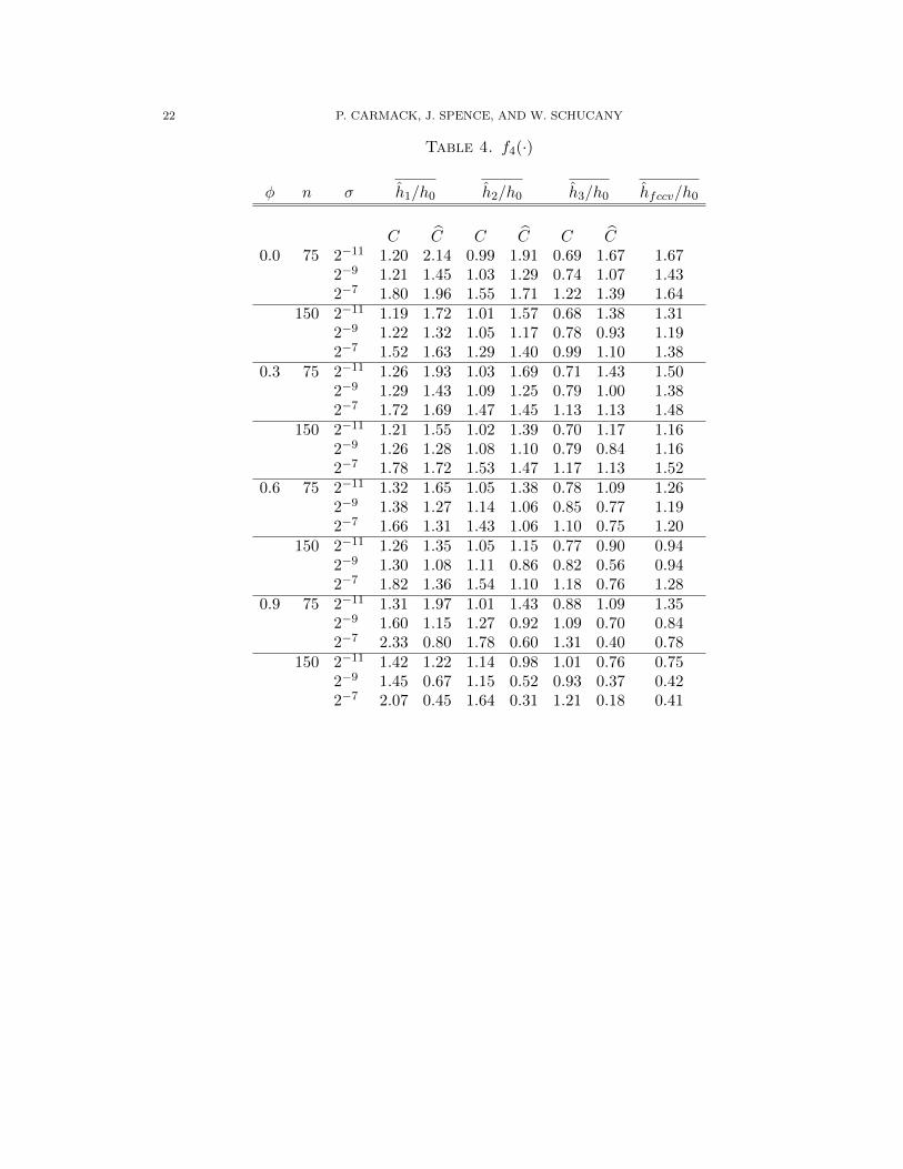
Table 4. f4(·)
φ n σ h1/h0 h2/h0 h3/h0 hfccv/h0
C C C C C C0.0 75 2−11 1.20 2.14 0.99 1.91 0.69 1.67 1.67
2−9 1.21 1.45 1.03 1.29 0.74 1.07 1.432−7 1.80 1.96 1.55 1.71 1.22 1.39 1.64
150 2−11 1.19 1.72 1.01 1.57 0.68 1.38 1.312−9 1.22 1.32 1.05 1.17 0.78 0.93 1.192−7 1.52 1.63 1.29 1.40 0.99 1.10 1.38
0.3 75 2−11 1.26 1.93 1.03 1.69 0.71 1.43 1.502−9 1.29 1.43 1.09 1.25 0.79 1.00 1.382−7 1.72 1.69 1.47 1.45 1.13 1.13 1.48
150 2−11 1.21 1.55 1.02 1.39 0.70 1.17 1.162−9 1.26 1.28 1.08 1.10 0.79 0.84 1.162−7 1.78 1.72 1.53 1.47 1.17 1.13 1.52
0.6 75 2−11 1.32 1.65 1.05 1.38 0.78 1.09 1.262−9 1.38 1.27 1.14 1.06 0.85 0.77 1.192−7 1.66 1.31 1.43 1.06 1.10 0.75 1.20
150 2−11 1.26 1.35 1.05 1.15 0.77 0.90 0.942−9 1.30 1.08 1.11 0.86 0.82 0.56 0.942−7 1.82 1.36 1.54 1.10 1.18 0.76 1.28
0.9 75 2−11 1.31 1.97 1.01 1.43 0.88 1.09 1.352−9 1.60 1.15 1.27 0.92 1.09 0.70 0.842−7 2.33 0.80 1.78 0.60 1.31 0.40 0.78
150 2−11 1.42 1.22 1.14 0.98 1.01 0.76 0.752−9 1.45 0.67 1.15 0.52 0.93 0.37 0.422−7 2.07 0.45 1.64 0.31 1.21 0.18 0.41

GENERALIZED CROSS-VALIDATION FOR CORRELATED DATA (GCVc) 23
ASEratio
φ
C Cσ = 1/2048
σ = 1/512
σ = 1/128
0.0 0.2 0.4 0.6 0.8
1.0
1.5
2.0
2.5
3.0
3.5
!!
!
!
0.0 0.2 0.4 0.6 0.8
1.0
1.5
2.0
2.5
3.0
3.5
!
! !
!
0.0 0.2 0.4 0.6 0.8
1.0
1.2
1.4
1.6
1.8
2.0
!
!!
!
0.0 0.2 0.4 0.6 0.8
1.0
1.2
1.4
1.6
1.8
2.0
!
! !
!
0.0 0.2 0.4 0.6 0.8
1.0
1.2
1.4
1.6
1.8
2.0
2.2
!
!
!
!
!
FCCVGCVc
(1)
GCVc(2)
GCVc(3)
0.0 0.2 0.4 0.6 0.8
1.0
1.2
1.4
1.6
1.8
2.0
2.2
! ! ! !
!
FCCVGCVc
(1)
GCVc(2)
GCVc(3)
Figure 7. Plots of the mean ASE ratios versus the AR(1) coefficient, φ,for the simulations using f2(·) and n = 75 for the methods indicated inthe legends. The means were formed by taking the average of the ratio ofeach method’s ASE over the optimal ASE for each of the 1,000 realizations.The rows are arranged by variance from low to high, top to bottom. Thecolumns indicate whether the known correlation matrix, C, was used, or itsnonparametric semivariogram estimate, C.
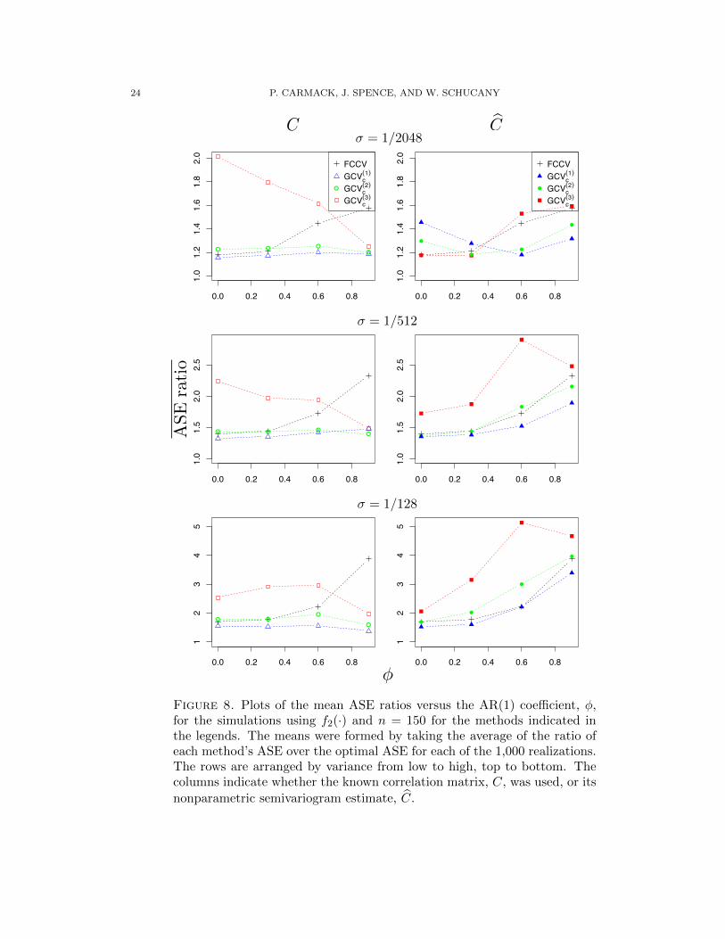
24 P. CARMACK, J. SPENCE, AND W. SCHUCANY
ASEratio
φ
C Cσ = 1/2048
σ = 1/512
σ = 1/128
0.0 0.2 0.4 0.6 0.8
12
34
5
!
!
!
!
0.0 0.2 0.4 0.6 0.8
12
34
5
! !!
!
0.0 0.2 0.4 0.6 0.8
1.0
1.5
2.0
2.5
!!
!
!
0.0 0.2 0.4 0.6 0.8
1.0
1.5
2.0
2.5
! ! !!
0.0 0.2 0.4 0.6 0.8
1.0
1.2
1.4
1.6
1.8
2.0
!
!!
!
!
FCCVGCVc
(1)
GCVc(2)
GCVc(3)
0.0 0.2 0.4 0.6 0.8
1.0
1.2
1.4
1.6
1.8
2.0
! ! !!
!
FCCVGCVc
(1)
GCVc(2)
GCVc(3)
Figure 8. Plots of the mean ASE ratios versus the AR(1) coefficient, φ,for the simulations using f2(·) and n = 150 for the methods indicated inthe legends. The means were formed by taking the average of the ratio ofeach method’s ASE over the optimal ASE for each of the 1,000 realizations.The rows are arranged by variance from low to high, top to bottom. Thecolumns indicate whether the known correlation matrix, C, was used, or itsnonparametric semivariogram estimate, C.
GENERALIZED CROSS-VALIDATION FOR CORRELATED DATA (GCVc) 25
ASEratio
φ
C Cσ = 1/2048
σ = 1/512
σ = 1/128
0.0 0.2 0.4 0.6 0.8
1.0
1.2
1.4
1.6
1.8
!!
!
!
0.0 0.2 0.4 0.6 0.8
1.0
1.2
1.4
1.6
1.8
!!
!
!
0.0 0.2 0.4 0.6 0.8
1.0
1.2
1.4
1.6
1.8
!
!
!!
0.0 0.2 0.4 0.6 0.8
1.0
1.2
1.4
1.6
1.8
!! !
!
0.0 0.2 0.4 0.6 0.8
1.0
1.5
2.0
2.5
3.0
3.5
!
!
!
!
!
FCCVGCVc
(1)
GCVc(2)
GCVc(3)
0.0 0.2 0.4 0.6 0.8
1.0
1.5
2.0
2.5
3.0
3.5
! ! ! !
!
FCCVGCVc
(1)
GCVc(2)
GCVc(3)
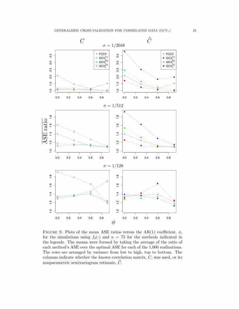
Figure 9. Plots of the mean ASE ratios versus the AR(1) coefficient, φ,for the simulations using f3(·) and n = 75 for the methods indicated inthe legends. The means were formed by taking the average of the ratio ofeach method’s ASE over the optimal ASE for each of the 1,000 realizations.The rows are arranged by variance from low to high, top to bottom. Thecolumns indicate whether the known correlation matrix, C, was used, or itsnonparametric semivariogram estimate, C.

26 P. CARMACK, J. SPENCE, AND W. SCHUCANY
ASEratio
φ
C Cσ = 1/2048
σ = 1/512
σ = 1/128
0.0 0.2 0.4 0.6 0.8
1.0
1.4
1.8
2.2
!
!
!!
0.0 0.2 0.4 0.6 0.8
1.0
1.4
1.8
2.2
!! !
!
0.0 0.2 0.4 0.6 0.8
1.0
1.2
1.4
1.6
!
!!
!
0.0 0.2 0.4 0.6 0.8
1.0
1.2
1.4
1.6
!! !
!
0.0 0.2 0.4 0.6 0.8
1.0
1.5
2.0
2.5
!
!
!!
!
FCCVGCVc
(1)
GCVc(2)
GCVc(3)
0.0 0.2 0.4 0.6 0.8
1.0
1.5
2.0
2.5
! ! ! !
!
FCCVGCVc
(1)
GCVc(2)
GCVc(3)
Figure 10. Plots of the mean ASE ratios versus the AR(1) coefficient, φ,for the simulations using f3(·) and n = 150 for the methods indicated inthe legends. The means were formed by taking the average of the ratio ofeach method’s ASE over the optimal ASE for each of the 1,000 realizations.The rows are arranged by variance from low to high, top to bottom. Thecolumns indicate whether the known correlation matrix, C, was used, or itsnonparametric semivariogram estimate, C.
GENERALIZED CROSS-VALIDATION FOR CORRELATED DATA (GCVc) 27
ASEratio
φ
C Cσ = 1/2048
σ = 1/512
σ = 1/128
0.0 0.2 0.4 0.6 0.8
1.0
1.5
2.0
2.5
!
!
!!
!
FCCVGCVc
(1)
GCVc(2)
GCVc(3)
0.0 0.2 0.4 0.6 0.8
1.0
1.5
2.0
2.5
! ! !!
!
FCCVGCVc
(1)
GCVc(2)
GCVc(3)
0.0 0.2 0.4 0.6 0.8
1.0
1.2
1.4
1.6
1.8
!! !
!
0.0 0.2 0.4 0.6 0.8
1.0
1.2
1.4
1.6
1.8
! ! !
!
0.0 0.2 0.4 0.6 0.8
1.0
1.5
2.0
2.5
! ! !
!
0.0 0.2 0.4 0.6 0.8
1.0
1.5
2.0
2.5
!!
!
!
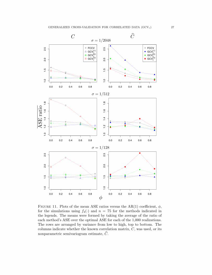
Figure 11. Plots of the mean ASE ratios versus the AR(1) coefficient, φ,for the simulations using f4(·) and n = 75 for the methods indicated inthe legends. The means were formed by taking the average of the ratio ofeach method’s ASE over the optimal ASE for each of the 1,000 realizations.The rows are arranged by variance from low to high, top to bottom. Thecolumns indicate whether the known correlation matrix, C, was used, or itsnonparametric semivariogram estimate, C.

28 P. CARMACK, J. SPENCE, AND W. SCHUCANY
ASEratio
φ
C Cσ = 1/2048
σ = 1/512
σ = 1/128
0.0 0.2 0.4 0.6 0.8
1.0
1.2
1.4
1.6
!
!
!!
!
FCCVGCVc
(1)
GCVc(2)
GCVc(3)
0.0 0.2 0.4 0.6 0.8
1.0
1.2
1.4
1.6
! !!
!
!
FCCVGCVc
(1)
GCVc(2)
GCVc(3)
0.0 0.2 0.4 0.6 0.8
1.0
1.2
1.4
1.6
1.8
! ! !
!
0.0 0.2 0.4 0.6 0.8
1.0
1.2
1.4
1.6
1.8
!!
! !
0.0 0.2 0.4 0.6 0.8
1.0
1.5
2.0
2.5
3.0
!
!!
!
0.0 0.2 0.4 0.6 0.8
1.0
1.5
2.0
2.5
3.0
!
!
!
!
Figure 12. Plots of the mean ASE ratios versus the AR(1) coefficient, φ,for the simulations using f4(·) and n = 150 for the methods indicated inthe legends. The means were formed by taking the average of the ratio ofeach method’s ASE over the optimal ASE for each of the 1,000 realizations.The rows are arranged by variance from low to high, top to bottom. Thecolumns indicate whether the known correlation matrix, C, was used, or itsnonparametric semivariogram estimate, C.