Embed Size (px)
Citation preview

Generalised single particle models for high-rateoperation of graded lithium-ion electrodes: systematic
derivation and validation
G. Richardson1,2,5, I. Korotkin1,2,6, R. Ranom3, M. Castle4, and J. M.Foster2,4,7
1Mathematical Sciences, University of Southampton, University Rd., SO171BJ, UK
2The Faraday Institution, Quad One, Becquerel Avenue, Harwell Campus,Didcot, OX11 0RA, UK
3Faculty of Electrical Engineering, Universiti Teknikal Malaysia Melaka,76100 Melaka, Malaysia
4School and Mathematics and Physics, University of Portsmouth, LionTerrace, PO1 3HF, UK
[email protected]@soton.ac.uk
July 23, 2019
Abstract
A derivation of the single particle model (SPM) is made from a porous electrodetheory model (or Newman model) of half-cell (dis)charge for an electrode composedof uniformly sized spherical electrode particles of a single chemistry. The derivationuses a formal asymptotic method based on the disparity between the size of the ther-mal voltage and that of the characteristic change in overpotential that occurs during(de)lithiation. Comparison is made between solutions to the SPM and to the porouselectrode theory (PET) model for NMC, graphite and LFP. These are used to identifyregimes where the SPM gives accurate predictions. For most chemistries, even at mod-erate (dis)charge rates, there are appreciable discrepancies between the PET modeland the SPM which can be attributed to spatial non-uniformities in the electrolyte.This motivates us to calculate a correction term to the SPM. Once this has been in-corporated into the model its accuracy is significantly improved. Generalised versionsof the SPM, that can describe graded electrodes containing multiple electrode particlesizes (or chemistries), are also derived. The results of the generalised SPM, with the
1
arX
iv:1
907.
0941
0v1
[ph
ysic
s.ch
em-p
h] 2
6 Ju
n 20
19
correction term, compare favourably to the full PET model where the active electrodematerial is either NMC or graphite.
1 Introduction
Lithium-ion batteries (LIBs) provide rechargeable energy storage at an unrivalled energyand power density, with a high cell voltage, and a slow loss of charge when not in use [3].These characteristics mean that they are already ubiquitous in the consumer electronicssector and are being increasingly adopted for use in electric vehicles and off grid storage.However, particularly for vehicular propulsion, there are still major hurdles to be overcome interms of lengthening service life, facilitating higher (dis)charge rates, and improving safety,particularly in high-rate regimes [36, 37]. Driven largely by the incumbent legislation to banthe combustion engine across large parts of the world before 2040, it has been predicted thatthe demand for LIBs will balloon from 45GWh/year (in 2015) to one of 390GWh/year in2030 [41] and so improvements in LIB performance are needed as a matter of urgency.
A LIB pack is comprised of a collection of single electrochemical cells. Within each ofthese cells are three main components which facilitate the electrochemical reactions drivingthe electrical current; they are, two electrodes and the electrolyte. Both the positive andnegative electrodes are themselves composites, being comprised of a porous network of mi-croscopic electrode particles and a conductive polymer binder. The voids within this solidscaffold are filled with liquid electrolyte. Lithium (Li) can be inserted into and extractedfrom the particulate electrode material (intercalated and deintercalated). During discharge,the Li is extracted from the negative electrode material forming a free electron and a Li+ ion.The ion is transported through the electrolyte (and separator diaphragm), and inserted intothe positive electrode material. This ionic current is compensated by a flow of free electronsthrough the external circuit providing the useful electrical current. The charging processoccurs similarly but with the ionic and electronic currents flowing in the opposite directions.
Modelling of LIB performance takes place over a wide range of length scales ranging fromatomistic scale simulations of battery materials to full device simulations and is reviewedby Franco in [16]. The current work is focussed on electrode scale modelling of LIBs andis based on the approach developed by Newman and his co-workers in the mid 90’s andearly 2000’s [10, 11, 17, 35] which is often referred to as porous electrode theory (PET). Theform of these models has since been justified using asymptotic homogenisation techniques in[31, 32]. In these models, partial differential equations for the Li concentration and electricpotentials are solved across the electrode. In order that source terms (which capture the(de)intercalation reactions) can be accurately evaluated, at each point in the macroscopicdimension (i.e. across the electrode) a microscopic problem is solved for the transport withinthe electrode particles. In the Newman group’s original work the electrode is assumed tohave a one-dimensional slab-like geometry and the electrode particles are assumed spher-ically symmetric. Hence, since both the macro- and microscopic problems are effectivelyone-dimensional, their work is often referred to as a pseudo-two-dimensional approach [18].The original PET works also choose to model lithium transport within the electrode par-ticles via a simple linear diffusion model. With recent improvements in the understandingof the chemistry of these active (electrode) materials it has become clear that a linear dif-
2

fusion model does not provide a good description of this transport process. Hence manyrecent works have focussed on incorporating more realistic lithium transport models in theactive materials into PET. These range from nonlinear diffusion models calibrated againstexperimental data [13, 12] to Cahn-Hilliard models for phase change materials [7, 9, 14].Here we will employ the former approach and restrict our attention to nonlinear diffusionmodels of lithium transport in the active materials. The original PET formulation has alsobeen generalised by posing the problem, on both macro- and micro-scales, in higher num-bers of dimensions. This enables the effects of electrode particle shape to be investigated,and also spatially inhomogeneities in electrode discharge that could arise, for example, fromnon-uniform heating or the positioning of the electrode tabs, see [15, 19].
Whilst it is difficult to overstate the success and utility of the PET approach, it can becriticised for being relatively expensive to solve. This is a particularly significant difficultywhen it is being used as a tool to optimise cell design [5], or extended to model to 2- or3-macroscopic dimensions [39, 8], or as a tool in parameter estimation studies [2, 33]. Itsmultiscale nature means that the underlying equations are posed over two separate spa-tial dimensions and, since these equations are nonlinear, obtaining solutions is a task thatneeds to be tackled numerically. This has motivated many authors to consider simplifiedversions of the PET. Perhaps the most well-known model of this type is the single particlemodel, or SPM, which results from assuming that each of the electrode particles are equallysized spheres, and then arguing that the electrochemical reactions occur roughly uniformlythroughout the electrodes so that the active material in the electrode particles (de)lithitatesat the same rate independent position in the electrode [22, 29]. In this way, finding modelsolutions is reduced to the task of solving a single spherical transport problem inside a ‘rep-resentative’ particle in each electrode. In this context we note that the thesis of Ranom [30],from which the current work stems, contains a systematic derivation of the leading orderSPM from the PET model.
After completion of this work, we became aware of another article in-progress that em-ploys asymptotic methods to simplify the PET model [21]. In [21], the asymptotic limit oflarge electrode and electrolyte conductivities and large electrolyte diffusivity is taken; thisis a different (and in fact complementary) limit to that taken here. Their limit recovers avariant of the SPM at leading order because the gradients in the electrolyte concentration,electrolyte potential, and electrode potentials are all small and this gives rise to homoge-neous behaviour of the electrode particles and hence leads to the SPM. In contrast, in ourlimit the variation in the overpotential across the electrode is small in comparison the typicalvariation in the equilibrium potential as lithium is removed/inserted into the electrode andit is this that leads to the SPM. Whilst both limits recover an SPM at leading order, thecorrection terms are different. If the model parameters for a particular case are not appro-priate for the limit considered here, we encourage the reader to also consider the reducedmodel in [21]. We also note the work of Moyles et al. [23] which also derives an asymptoticreduction of a PET model, but does so by first volume averaging lithium transport overthe electrode particles in the PET model, and thereby implicitly assumes transport withinindividual electrode particles is rapid.
In order to properly understand for which electrode chemistries it is appropriate to usethe SPM approximation we will, throughout this work, restrict our attention to half-cellconfigurations, noting that the extension to full cells is straightforward. Such half-cell con-
3

figurations are comprised of a single porous electrode (either a cathode or anode) being(dis)charged, through a separator, against a metallic Li counter electrode [26, 38], see figure1. We will allow the electrodes within our half-cells to contain more than one size of elec-trode particle and/or more than one chemistry, and this will allow us to derive generalisedversions of the SPM applicable to graded electrodes. Motivated by the need to provide auseful tool for the practitioner we validate our approximations, as far as possible, againstrealistic data sets for the PET model. Here these data sets are primarily based upon twoworks from the Ecker group [13, 12] which adopt a combined experimental and theoreticalapproach validating the results of their PET model simulations against data collected fromreal cells.
In the next section of the paper we describe the PET model as well as the boundaryand initial conditions with which it should be supplemented in order to mimic a half-cellconfiguration. Then, in §3 we describe a generalisation of the standard SPM that is applicableto graded electrodes and ones with multiple electrode particle chemistries. We also outlinehow higher order terms, which capture the effects of spatial and temporal variations in theelectrolyte properties, can be incorporated into this generalised SPM. Including these higherorder terms requires that a one-dimensional system of PDEs be solved in the electrolyte,in addition to the one-dimensional PDEs in the electrode particles. However introducingthis extra complexity into the simplified model significantly enhances its accuracy as wedemonstrate with the aid of some examples: (i) electrodes with a uniform particle size and(ii) graded electrodes with two sizes particle segregated into separate regions. In §4 weintroduce scalings and rewrite the PET in dimensionless form. This nondimensionalisationfacilitates the asymptotic analysis which is the subject of §5. Here, the SPM, as well as itsgeneralisised version for graded electrodes, and its higher order correction terms, is derivedsystematically from the PET. Finally, in §6 we draw our conclusions.
2 Problem formulation
Here, we consider a PET model posed on the model geometry shown in figure 1. Theequations governing ionic transport through the electrolyte are[6, 17, 30, 31]
εl(x)∂c
∂t+∂F−∂x
= 0, F− = −B(x)D(c)∂c
∂x− (1− t+)
j
Fin − Ls < x < L. (1)
where, x and t denote position through the electrode and time respectively, εl is the localvolume fraction of electrolyte, c is the molar concentration of ions (the Li and counter ionconcentrations are equal throughout the bulk owing to the extremely short Debye length ofthe solution) in the electrolyte, F− is the effective flux of anions across the electrolyte, Dis the ionic diffusivity of the electrolyte, B is the permeability factor (often estimated usingthe ad-hoc relation offered by Bruggeman which takes B = ε1.5l [4]), t+ is the transferencenumber, j is the ionic current density and F is Faraday’s constant. In contrast to some otherauthors, we opt to write the conservation equation in terms of the anion flux, F−, ratherthan the cation flux, F+. We make this choice, because the anion is not (de)intercalated intothe electrode particles and as a consequence its governing equation takes a conservative formwhich is more susceptible to the numerical treatment that we employ later in this work. This
4

would not be the case if the conservation equation is written for the lithium cation whichmust contain a source/sink terms to account for the (de)intercalation process. The ioniccurrent in the electrolyte obeys
∂j
∂x= Fb(x)G, j = −B(x)κ(c)
(∂φ
∂x− 2RT
F
1− t+
c
∂c
∂x
)in − Ls < x < L. (2)
Here b is the Brunauer-Emmett-Teller (BET) surface area (with units of 1/m), G is thereaction rate which is zero in the separator and given by the Butler-Volmer equations inthe electrode (where it is the flux per unit area of Li through the surface of the electrodeparticles), κ is the ionic conductivity, φ is the electric potential in the electrolyte, R is the(molar/universal/ideal) gas constant and T is absolute temperature. The electric transportthrough the solid scaffold is governed by
∂js∂x
= −Fb(x)G, js = −σ∂φs∂x
in 0 < x < L (3)
where φs, js and σ are the electric potential, current density and conductivity of the electrode.We will refer to equations (1)-(3) as the macroscopic equations because their independentspatial variable, x, measures the macroscopic distance across the thickness of the electrode(cf. figure 1).
Boundary conditions We will assume that the half-cell (dis)charges according to somespecified current supply/demand, I(t), and as such boundary conditions to supplement thesixth order system of PDEs posed on the macroscale, (1)-(3), require: (i) That the Li-metalsupplies an ionic current density of I(t)/A to the electrolyte in the separator (on x = −Ls).We further require, (ii), that at the current collector (x = L) there is injection of current ofdensity I(t)/A into the solid phase. In addition, (iii), no current flows from the solid phaseinto the separator at x = 0. A reference potential in the electrolyte is provided at the edgeof the separator where it meets the Li-metal (x = −Ls). Finally, (v) and (vi), we specifythat there should be no anion flux in the electrolyte at the interfaces where it meets boththe separator and current collector. In summary we have
j|x=−Ls =I(t)
A, F−|x=−Ls = 0, φ|x=−Ls = 0, (4)
js|x=0 = 0, js|x=L =I(t)
A, F−|x=L = 0. (5)
The Butler-Volmer reaction rate It remains to specify the reaction rate G. In theseparator (−Ls < x < 0), where there are no electrode particles, this is zero. In theelectrode (0 ≤ x < L) the reaction rate is determined by the Butler-Volmer (BV) equation[17, 24, 25] such that G is given by
G =
0 in −Ls < x < 0,
2kc1/2(cs|r=R(x)
)1/2 (cmaxs − cs|r=R(x)
)1/2sinh
(Fη
2RT
)in 0 ≤ x < L,
(6)
5

Figure 1: A schematic of the half cell geometry as well as the independent variables and snap-shot of their qualitative profiles during charging if the electrode is an anode, or dischargingif the electrode is a cathode.
where the overpotential is given by
η = φs − φ− Ueq(cs|r=R(x)). (7)
Here, Ueq, cmaxs and R(x) are the equilibrium potential, the maximum concentration of
lithium that can be stored in the electrode material, and the radii of electrode particles.
Equations on the microstructure Evaluating the (de)intercalation rates, G, necessi-tates solving for the solid-state lithium concentration on the surfaces of the electrode par-ticles throughout the electrode. Whilst there is considerable debate about the correct solidstate transport model, particularly for phases separating electrode materials [1, 20, 27], here,we opt to solve non-linear diffusion equations in the active material particles and as such wehave
∂cs∂t
=1
r2∂
∂r
(r2Ds(cs)
∂cs∂r
)in 0 < r < R(x) and 0 < x < L. (8)
Here Ds and r are the concentration-dependent diffusivity and radial coordinate withinthe particles respectively. Equations (8) are closed by supplying them with the boundaryconditions
cs bounded on r = 0, −Ds(cs)∂cs∂r
∣∣∣∣r=R(x)
= G. (9)
The former is a regularity conditions required to eliminate singular behaviour at the originwhilst the latter ensures that there is the requistite Li flux across the surface owing tothe reactions taking place there. We will refer to the (8)-(9) as the microscopic transportproblem.
6

The half-cell potential The half-cell potential, V , is given by the expression
V (t) = φs∣∣x=L
. (10)
Note that it is straightforward to include an Ohmic drop across the current collector interfacecaused by a contact resistance R by replacing this expression by one of the form V (t) =φs∣∣x=L−RI.
Initial conditions The parabolic equations (1) and (8) require initial conditions on theelectrolyte ion concentration c throughout the electrolyte as well as cs, the concentrationof Li in the electrode particles. We assume that the electrode is initially in equilibrium sothat both I(0) = 0 and G(x, 0) = 0. As such we require a uniform salt concentration in theelectrolyte
c∣∣t=0
= cinit in − Ls < x < L. (11)
and a uniform lithium concentration throughout all the electrode particles
cs∣∣t=0
= cs,init in 0 < r < R(x) and 0 < x < L. (12)
It follows from these conditions, and the model equations, that initially φ(x, 0) = 0 andφs(x, 0) = Ueq(cs,init).
Electrode geometry We assume that all electrode particles are spheres, with radii thatvary on the relatively long lengthscales assoiated with the macroscopic thickness (but noton the much shorter lengthscale of individual electrode particles, i.e., the microscale). Thisgives rise to the following relationship between the BET surface area, particle radius, andvolume fraction of electrode particles
εs(x) =b(x)R(x)
3, (13)
where εs is the local volume fraction of electrode particles. The relationship (13) follows fromnoting that the volume fraction of particles within a small representative elementary volumeis the product of the volume of a single particle, namely 4πR3, and the number of particleswithin the REV, namely b/(4πR2). The volume fraction, εs, is related to the volume fractionof liquid in the electrode via
εl(x) = 1− εinert(x)− εs(x), (14)
where εinert is the volume fraction of electrochemically inert material (e.g., polymer binderor the conductivity enhancing carbon black).
3 Results
We begin by stating the generalisation of the single particle model (SPM) approximationto graded electrodes. This is based on the assumption that U the characteristic change in
7

overpotential that occurs as lithium is intercalated into (or removed from) the electrodematerial is much larger than the thermal voltage VT = RT/F ≈ 26mV. Formally we require
λ 1 where λ =FURT
.
It is thus applicable to materials such as graphite, NMC or LCO (though not to LFP whereU ≤ 26mV). We then give a recipe for extending the SPM to incorporate further terms,which depend upon the electrolyte behaviour, and considerably enhance the accuracy of themethod. Henceforth we will refer to the corrected SPM, which includes the additional terms,as the ‘corrected SPM’. In order to illustrate the method we consider two examples. The firstof these (described in §3.1) is the single particle model which applies to electrodes comprisedof uniform sized electrode particles (i.e. with no grading) while the second (described in§3.2) is the double particle model which applies to electrodes which are graded with twoparticle sizes occupying different regions of the electrode (one near the separator and onenear the current collector). In both cases we compare results of the SPM and corrected SPMto the full numerical solution to the PET model (1)-(10) for electrodes of several differentchemistries. Derivation of the approximate models, from the PET model, is deferred until§5.
The leading order approximation. The most basic approximation to the Newmanmodel (1)-(10) in the scenario described above is the following generalisation of the SPM:
∂cs∂t
=1
r2∂
∂r
(r2Ds(cs)
∂cs∂r
)in 0 ≤ r ≤ R(x), (15)
cs bounded on r = 0, cs|r=R(x) = C(t), cs|t=0 = cs,init, (16)∫ L
0
b(x)G(x, t)dx =I(t)
AFwhere G = −Ds(cs)
∂cs∂r
∣∣∣∣r=R(x)
(17)
Here the function C(t) in (16) is chosen so that the integral constraint (17) is satisfied.The leading order approximation to the voltage, V (t), of the half-cell is calculated from thesolution of this problem (15)-(17) via the relation
V (t) ≈ Ueq(C(t)). (18)
A higher order approximation. A more accurate expression for V (t) can be calculatedfrom the solution to (15)-(17) but additionally requires a one-dimensional problem for theelectrolyte be solved. This expression reads
V (t) ≈ Ueq(C(t)) +
∫ L
0
b(x)R(x)
[η(x, t) + φ(x, t)−
∫ L
x
js(x′, t)
σ(x′)dx′]dx∫ L
0
b(x)R(x)dx
. (19)
8

Figure 2: Ionic diffusivity (top left) and conductivity (top right) of the electrolyte from [13],non-linear diffusivity of graphite (LiC6) anode (bottom left) and Li(Ni0.4Co0.6)O2 cathode(bottom right). Experimental data from [13] and approximate fits.
9
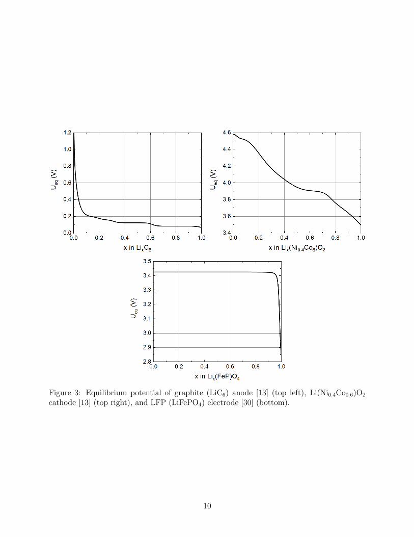
Figure 3: Equilibrium potential of graphite (LiC6) anode [13] (top left), Li(Ni0.4Co0.6)O2
cathode [13] (top right), and LFP (LiFePO4) electrode [30] (bottom).
10

Here φ(x, t), the potential in the electrolyte, and η(x, t), the associated overpotential, arecalculated from the solution to the one dimensional electrolyte problem
εl(x)∂c
∂t+∂F−∂x
= 0, F− = −B(x)D(c)∂c
∂x− (1− t+)
j
F, (20)
∂j
∂x= Fb(x)G(x, t), j = −B(x)κ(c)
(∂φ
∂x− 2RT
F
1− t+
c
∂c
∂x
), (21)
with
j|x=−Ls =I(t)
A, F−|x=−Ls = 0, φ|x=−Ls = 0, F−|x=L = 0, (22)
and c|t=0 = cinit, (23)
where
js(x, t) =I
A− j(x, t), η(x, t) = 2
RT
Farcsinh
(G(x, t)
2k[(cmaxs − C(t))C(t)c]1/2
), (24)
and G(x, t) is obtained from the solution to the leading order problem (15)-(17). Notablythe approximated expression for V (t) calculated in (19) is a formally accurate approximationto the PET model (1)-(10) (as explained in §5), for all discharge rates, in the case that theelectrode is composed of uniformly sized particles of a single material. However, even wherethis is not the case (e.g. if the electrode is graded), it is still formally accurate provided thatthe (dis)charge rate is not excessively large in comparison to the characteristic timescalefor transport within the electrode particles. More specifically, it is still formally accurateprovided
Q 1 where 3Q =timescale for Li diffusion into electrode particle
timescale for cell discharge.
The dimensionless parameter Q will be defined rigorously below in §4. Since this require-ment is usually satisfied, even at moderate to aggressive discharge rates, it usually offers asignificant improvement over the leading order approximation (18).
3.1 The Single Particle Model and comparison to the PET model
In the case where all the electrode particles are of uniform size R, across the width of theelectrode the leading order equations (15)-(17) simplify considerably since cs = cs(r, t) andG = G(t) so that in this case we need solve only a single microscopic transport problem inr, namely (15) subject to the boundary conditions
cs bounded on r = 0, Ds(cs)∂cs∂r
∣∣∣∣r=R
= −G(t) where G(t) =I(t)
AF∫ L0b(x)dx
, (25)
from which we can then evaluate
C(t) = cs|r=R (26)
11
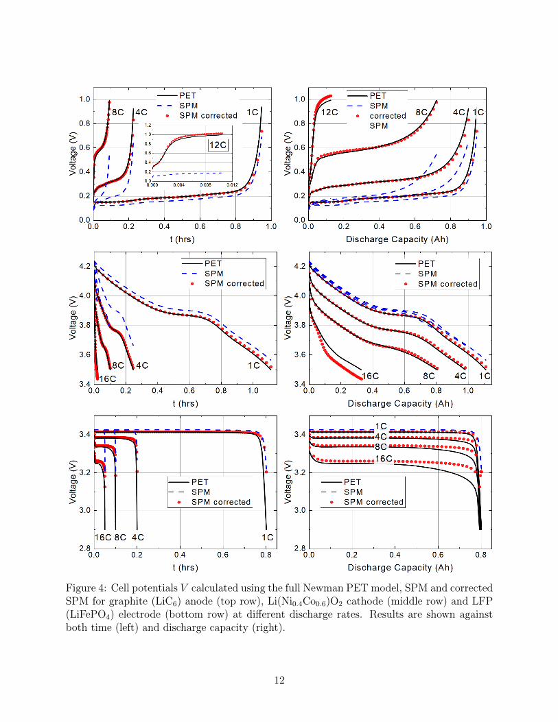
Figure 4: Cell potentials V calculated using the full Newman PET model, SPM and correctedSPM for graphite (LiC6) anode (top row), Li(Ni0.4Co0.6)O2 cathode (middle row) and LFP(LiFePO4) electrode (bottom row) at different discharge rates. Results are shown againstboth time (left) and discharge capacity (right).
12

Figure 5: Concentration of Li+ ions (top left) and potential (top right) in the electrolyteacross a half-cell with a Li(Ni0.4Co0.6)O2 electrode calculated using the PET model and theleading order electrolyte equations, (20)-(24), at 8C discharge rate. In the upper panels asingle snapshot in time (at the end of discharge) is shown because the electrolyte approachesa steady-state rapidly and hence the profiles at earlier times look very similar to thoseshown. Concentration of Lithium on the electrode particle surfaces (bottom left) and thepotential in the solid (bottom right) across the Li(Ni0.4Co0.6)O2 electrode calculated usingthe full Newman PET at 8C discharge rate. Arrows indicates the direction of increasingtime and plots are made at 20 evenly spaced times between 0 and 0.10 hrs. The leadingorder electrolyte equations are used to evaluate the first order terms in the corrected SPM,see (19).
13

and use the functions G(t) and C(t) thus determined as inputs in the electrolyte model (20)-(24) which we can then solve to obtain the data necessary to compute the corrected voltagevia (19).
Simulations of both the basic SPM and its more accurate extension, the corrected SPM,are compared to simulations of the full PET model in figure 4 as discharge curves showingcell voltage V (t) plotted against time t in the left-hand panels and V (t) plotted againstcapacity in the right-hand panel. We examine three different electrode chemistries, namely,(i) a graphite anode LiC6, (ii) an NMC nickel-cobalt oxide cathode Li(Ni0.4Co0.6)O2 and(iii) an LFP lithium-iron phosphate LiFePO4 cathode. The parameter values for the formertwo of these are taken from the work of Ecker et. al [13, 12] whilst the latter are takenfrom Ranom [30]. The open circuit voltages Ueq(cs) for all three materials are fitted to datafrom [13, 12, 30] in figure 3, while the electrolyte diffusion coefficient D(c) and the electrolyteconductivity κ(c), for all three electrodes, is fitted to data in [13, 12] in figure 2 (top). Finallythe active material diffusion coefficient Ds(cs) for the graphite and NMC particles are fittedto data from [13, 12] in figure 2 (bottom). Diffusion in the LFP nanoparticles is modelledby a linear diffusion equation with diffusion coefficient Ds = 9 × 10⁻¹⁴m2s−1 as in Table 1(this is so fast and the particles so small that diffusion is effectively instantaneous). Allother parameter values are tabulated in Tables 1 and 2. Figure 5 shows electrolyte variables(c upper left panel and φ upper right panel) plotted as a function of distance x across thehalf cell in addition to lithium concentration on the particle surfaces cs|r=R (lower left panel)and electrode potential φs (lower right panel), all for an 8C discharge of the Li(Ni0.4Co0.6)O2
half-cell.We observe that the basic SPM, reliably reproduces the results of the full PET across a
range of chemistries provided that the rates are relatively low, i.e., less than 1C or so. Asdischarge rates increase beyond around 1C the accuracy of the SPM deteriorates. However,if the correction terms are accounted for, the range of accuracy of the SPM can be expandedsignificantly. In particular, for graphite, the results of full PET and the corrected SPM arealmost indistinguishable even up to the relatively aggresive rate of 12C. For NMC and LFPelectrodes, excellent agreement between the PET and corrected SPM is maintained untilaround 16C and 4C respectively. Beyond these values, even the corrected SPM begins to benoticeably different from the PET model, but, still performs far better than the usual SPMapproximation.
As we will discuss in more detail in §5 the reliability of the corrected SPM is intimatelylinked to the characteristic size in the change of the overpotential of the electrode materialas it is (de)lithiated. In particular it is surprising that good agreement is obtained betweenthe corrected SPM and the PET model in the case of the LFP electrode because formallythe SPM derivation, as we shall show in §5, should not apply to a material with such a flatdischarge curve.
14
3.2 The Double Particle Model and comparison to the Newmanmodel
If instead of an electrode comprised of just one size of electrode particle we consider anelectrode composed of two sizes of particle distributed in space so that
R(x) =
R(a) for 0 ≤ x < αR(b) for α ≤ x < L
, (27)
we find that the leading order equations (15)-(17) reduce to the double particle model
∂c(a)s
∂t=
1
r2∂
∂r
(r2Ds(c
(a)s )
∂c(a)s
∂r
)in 0 ≤ r ≤ R(a)
c(a)s bounded on r = 0, c
(a)s
∣∣∣r=R(a)
= C(t)
, c(a)s |t=0 = cs,init, (28)
∂c(b)s
∂t=
1
r2∂
∂r
(r2Ds(c
(b)s )
∂c(b)s
∂r
)in 0 ≤ r ≤ R(b),
c(b)s bounded on r = 0, c
(b)s
∣∣∣r=R(b)
= C(t),
, c(b)s |t=0 = cs,init, (29)
∫ α
0
b(x)
(Ds(c
(a)s )
∂c(a)s
∂r
)∣∣∣∣∣r=R(a)
dx+
∫ L
α
b(x)
(Ds(c
(b)s )
∂c(b)s
∂r
)∣∣∣∣∣r=R(b)
dx =I(t)
AF. (30)
Once these have been solved, the functions G(t) and C(t) can, once again, be used as inputsin the electrolyte model (20)-(24) which we can then solve to obtain the data necessary tocompute the voltage according to the corrected SPM, i.e. via (19).
Figures 6 compare the results of this double particle model, both without the correctionterm (DPM) and with the correction term (DPM corrected), to the PET model. Here wetake α = L/2 and R(a) = 4R(b), b(a) = b(b)/4 in all three cases while R(b) and b(b) are givenby the values of R0 and b0 in Table 1 for the appropriate chemistries. Figure 7 shows theequivalent electrolyte variables (c upper left panel and φ upper right panel) plotted as afunction of distance x across the half cell in addition to lithium concentration on the particlesurfaces cs|r=R(x) (lower left panel) and electrode potential φs (lower right panel), all for an8C discharge of the graded Li(Ni0.4Co0.6)O2 half-cell.
We note that the inclusion of the first order correction terms into the model (i.e. up-grading to the corrected DPM) in figure 6 significantly improves the agreement with the fullPET simulation over that with the simple DPM throughout the range of (dis)charge ratesand chemistries we explored . Notably in the case of the LFP half-cell the agreement ofDPM corrected with the PET simulations is not as good as it was for the electrode withsingle particle size. However some discrepancy is to be expected between the corrected DPMmodel and the PET model for an electrode formed from an active material with such a flatdischarge curve.
4 Nondimensionalisation of the model
Before applying asymptotic methods to derive the approximate models described in (15)-(24)from the underlying Newman model (1)-(10) we must non-dimensionalise the PET model. A
15

Figure 6: Cell potentials V calculated using the full PET model, DPM and the correctedDPM for graphite (LiC6) anode (top row), Li(Ni0.4Co0.6)O2 cathode (middle row) and LFP(LiFePO4) electrode (bottom row) at different discharge rates. Results are shown againstboth time (left) and discharge capacity (right).
16

Figure 7: Concentration of Li+ ions (top left) and potential (top right) in the electrolyteacross a half-cell with an Li(Ni0.4Co0.6)O2 electrode formed from particles of two differentsizes and calculated using the full PET model and the leading order approximation at 4Cdischarge rate. In the upper panels a single snapshot in time (at the end of discharge) isshown because the electrolyte approaches a steady-state rapidly and hence the profiles atearlier times look very similar to those shown. Concentration of Li on the particle surfaces(bottom left) and potential in solid (bottom right) across an Li(Ni0.4Co0.6)O2 electrode withtwo different particle sizes calculated using the full PET model at 4C discharge rate. Arrowsindicates the direction of increasing time and plots are made at 20 evenly spaced timesbetween 0 and 0.19 hrs.
17

key quantity, that will be used later for our temporal scaling, is τ the characteristic timescalefor cell (dis)charge, i.e., the characteristic timescale over which an electrode can sustain acurrent of size, I. This is
τ =ALFcmax
s bR
I, (31)
where I, b and R are typical sizes of the I, b and R respectively. The timescale τ canbe directly assessed by examining typical C-rates used for battery discharge. Here, we willexamine a range of C-rates from the relatively mild (1C, corresponding to a half cycle time of1hour) to the relatively aggresive (16C, corresponding to a half cycle time of 3.75 minutes).
The spatial coordinate x is scaled based on the width of the electrode L. The quantitiesc, cs, R, D, Ds, κ, I, B, σ and b are scaled with their typical values, namely cinit, c
maxs , R, D,
Ds, κ, I, B, σ and b respectively. The BV reaction rate will be scaled based on the averageflux required through particle surfaces to sustain a current of size I. The scaling for theeffective ionic flux is based on the size of the diffusive flux carried by a concentration of sizecinit over lengths of size L with an effective diffusivity of size BD.
It remains to specify scalings for the various different potentials. One natural scale is thatof the variation of the electric potential within the electrolyte. The conductivities of typicalelectrolytes are chosen so that only small variations in potential, on the order of the thermalvoltage RT/F = 26mV, are sufficient to carry the requisite current densities suggesting thatan appropriate scaling for φ is the thermal voltage. A second natural potential scale, whichwe will henceforth refer to as the characteristic half cell voltage, U , is the size of the differencebetween the overpotentials of a fully lithiated electrode particle and that of a fully delithiatedone. The overpotential of graphite varies between around 0V at full lithiation and 1V at fulldelithiation whilst the various metal oxides used in cathodes, e.g. NMC, exhibit variationsin their overpotentials of 3V at full lithation and 4V at full delithitaion. We proceed onthe basis that a typical value the characteristic cell potential, U can be taken to be on theorder of 1V. A notable exception if LFP which exhibits a extremly flat discharge curve forwhich U ≤ 26mV. In order that the reaction rates on the particle surfaces are of the requisitesize to satitate a current demand of size I we should scale both the electrode overpotential,Ueq, and the solid electrode potential, φs, with the characteristic cell voltage. It is the vastdisparity between the thermal voltage and the characteristic cell voltage that gives rise tothe large value of the dimensionless parameter λ and facilitates the asymptotic analysis thatjustifies the SPM derivation. In summary, our scalings for the problem are
t = τt∗ x = Lx∗ r = Rr∗ D = DD∗ (32)
Ds = DsD∗s κ = κκ∗ c = cinitc
∗ cs = cmaxs c∗s (33)
V = UV ∗ φ =RT
Fφ∗ φs = Uφ∗s j =
I
Aj∗ (34)
js =I
Aj∗s I = II∗ G =
I
ALF bG∗ η =
RT
Fη∗ (35)
Ueq = UU∗eq F− =BDcinitLF∗− B = BB∗ b = bb∗ (36)
I = II∗ R = RR∗ σ = σσ∗. (37)
18

The non-dimensionalisation gives rise to the following dimensionless quantities that charac-terise the system:
N =L2
τ BD, Γ =
IL
AcinitDBF, λ =
UFRT
, Q =R2
τDs
, (38)
Υ =kcs,init
1/2cmaxs ALF b
I, Θ =
σRTA
LIF, P =
BκRTALIF
, Ls =LsL
(39)
cs,init =cs,initcmaxs
. (40)
Of those parameters whose meaning is not self-evident from their definition; N is thetimescale for diffusion in the electrolyte over the timescale for cell discharge, Γ is the driftflux over the diffusive flux, Q is the timescale for diffusive transport inside the electrodeparticles over the timescale for cell discharge, Υ is the total amount of lithium intercalatedinto the active material per second over the current, Θ is the electronic conductivity of thesolid scaffold over the characteristic conductivity of the electrode material, P is the ionicconductivity over the characteristic conductivity of the electrode material.
4.1 The Half-Cell Dimensionless Model
On dropping the stars from the dimensionless variables the dimensionless problem reads asfollows. In the region −Ls < x < 0 the (dimensionless) electrolyte equations are
εl(x)N ∂c
∂t+∂F−∂x
= 0, F− = −B(x)D(c)∂c
∂x− Γ(1− t+)j, (41)
∂j
∂x=
0 for −Ls < x < 0b(x)G(x, t) for 0 < x < 1
, (42)
j = −Pκ(c)B(x)
(∂φ
∂x− 2
1− t+
c
∂c
∂x
), (43)
and satisfy the boundary conditions
j|x=−Ls = I(t), F−|x=−Ls = 0, φ|x=−Ls = 0, F−|x=1 = 0. (44)
These couple to the (dimensionless) electrode equations in the region 0 < x < 1
js = −λΘσ∂φs∂x
,∂js∂x
= −b(x)G(x, t), (45)
G(x, t) = 2Υc1/2(cs|r=R(x)
)1/2 (1− cs|r=R(x)
)1/2sinh
(η2
), (46)
η = λ(φs − Ueq(cs|r=R(x))
)− φ, (47)
Q∂cs∂t
=1
r2∂
∂r
(r2Ds(cs)
∂cs∂r
), for 0 ≤ r ≤ R(x), (48)
cs bounded on r = 0, −Ds∂cs∂r
∣∣∣∣r=R(x)
= QG. (49)
19

Table 1: Parameter values used in the model for different chemistries
Parameter UnitsGraphite (LiC6)
[12, 13]Li(Ni0.4Co0.6)O2
[12, 13]LFP (LiFePO4)
[30, 40]
Electrode thickness, L µm 74 54 62
Electrode particle radius, R0 µm 13.7 6.5 0.05
Electrode cross-section area, A m2 8.585× 10⁻³ 8.585× 10⁻³ 10−4
Vol. fraction electrolyte, εl – 0.329 0.296 0.4764
Brunauer-Emmett-Tellersurface area, b0 = 3(1− εl)/R0
m−1 1.469× 10⁵ 3.249× 10⁵ 3.142× 10⁷
Conductivity in solid, σ0 S m−1, 14.0 68.1 0.5
Permeability factor ofelectrolyte, B0
– 0.162 0.153 0.329
Reaction rate constant, k m2.5s−1mol−0.5 2.333× 10⁻¹⁰ 5.904× 10⁻¹¹ 3× 10⁻¹²
Maximum concentration ofLi ions in solid, cmax
s
mol m−3 17715.6 28176.4 18805
Transference number, t+ – 0.26 0.26 0.3
1C current draw, I0 A -0.15625 0.15625 0.0015
Contact resistance, Rc Ω 0 0 0
Absolute temperature, T K 298.15 298.15 298.15
Typical concentration of Liin liquid, cinit
mol m−3 1000 1000 1000
Typical diffusivity liquid, D0 m2s−1 2.594× 10⁻¹⁰ 2.594× 10⁻¹⁰ 2.594× 10⁻¹⁰
Typical conductivity liquid, κ0 S m−1 1.0 1.0 1.0
Diffusivity in solid, Ds m2s−1 Fig.2 Fig.2 9× 10⁻¹⁴
Typical diffusivity in solid, D0 m2s−1 3× 10⁻¹⁴ 10−13 9× 10⁻¹⁴
Equilibrium potential, Ueq V Fig.3 Fig.3 Fig.3
Characteristic cell voltage, U V 1.0 1.0 1.0
Discharge time scale (31), τ s 1.399× 10⁴ 1.703× 10⁴ 1.178× 10⁴
Derived dimensionless quantities (38)-(40)
N = L2/(τ BD) – 0.0093 0.0043 0.0038
Γ = I0L/(AcinitDBF ) – 0.332 0.257 0.113
Υ = kc1/2initc
maxs ALF b/I – 7.53 4.89 22.4
Θ = σRTA/(LIF ) – 267 1780 13.8
P = BκRTA/(LIF ) – 3.1 4.0 9.1
Q = R2/τDs – 0.447 0.0248 2.36× 10⁻⁶
20

Table 2: Parameters of the separator used in the model
Parameter Units Separator [34]
Thickness, Lsep µm 25
Volume fraction of electrolyte, εsepl – 0.55
Permeability factor of electrolyte, Bsep0 – 0.408
which in turn satisfy two boundary conditions in x, namely
js|x=0 = 0, js|x=1 = I(t), V (t) = φs|x=1. (50)
The final condition in (50) serves to determine the half-cell voltage V (t) from the solution tothe problem. Initial conditions corresponding to a half-cell which is initially at equilibriumare
c|t=0 = 1, cs|t=0 = cs,init. (51)
where cs,init is uniform throughout the cell (i.e. is independent of both x and r).
Features of the model Some helpful features of the model can be derived by taking thesum of equations (42) and (45b) in the region 0 < x < 1, integrating the results and applyingthe boundary conditions (44d) and (50b). We arrive at
j + js = I(t). (52)
Thus, the total (both ionic and electronic) current density is uniform throughout the elec-trode. Furthermore, on integrating (42) through the thickness of the electrode (−Ls < x < 1)and applying the boundary conditions (44a) and (44d) we obtain the integral condition∫ 1
0
b(x)G(x)dx = −I(t). (53)
This amounts to the observation that the total amount of charge (de)intercalating within theelectrode is in balance with the charge being deliver to/supplied from the external circuit.
5 Asymptotic reduction: derivation of single and mul-
tiple particle models
In this section we systematically derive both the basic SPM and the corrected SPM for thehalf cell from the dimensionless PET model (41)-(50) using asymptotic methods in the largeλ limit. In addition to deriving these SPMs we also derive natural extensions that describeelectrodes with more than one particle size and/or chemistry. This analysis can easily beextended to a full-cell, with two porous electrodes, but we do not do this here. Formally we
21

investigate the distinguished limit in which λ → ∞ and all other dimensionless parameters(i.e. N , Γ, Ls, P , Θ, Υ, cs,init and Q) are order 1.
The key observation that leads to the SPM is that in order that the dimensionless currentI(t) is of size O(1) the total amount of intercalation throughout the electrode must also besize O(1) (see (53)). In turn this requires that, the dimensionless overpotential, η is O(1)throughout the electrode which leads to the condition that
φ− λ(φs − Ueq(cs|r=R(x))
)= O(1). (54)
Since I(t) is O(1) it follows that both the dimensionless current densities j and js, within theelectrolyte and electrode respectively, are O(1). The condition that j = O(1) and equation(44) imply that φ = O(1) while the condition that js = O(1) means that gradients in φs areO(1/λ). This leads us to the following asymptotic expansion:
φs = φs,0 +1
λφs,1 + · · · , V = V0(t) +
1
λV1(t) + · · · , cs = cs,0 +
1
λcs,1 · · · ,
js = js,0 +1
λjs,1 · · · , ηi = η0 +
1
λη1 · · · , Gi = G0 +
1
λG1 · · · ,
φ = φ0 + · · · , c = c0 + · · · j = j0 + · · · ,F− = F−,0 + · · · .
(55)
The leading order problem. The derivation of the leading order term presented herebroadly follows that in the thesis of Ranom [30]. On inserting the expansions (55) into theequations (45)-(50) and taking the leading order terms we obtain the following problem in0 ≤ x ≤ 1:
∂φs,0∂x
= 0, (56)
∂js,0∂x
= −b(x)G0(x, t), js,0|x=0 = 0, js,0|x=1 = I(t), (57)
φs,0 = Ueq
(cs,0|r=R(x)
), V0(t) = φs,0|x=1, (58)
Q∂cs,0∂t
=1
r2∂
∂r
(r2Ds(cs,0)
∂cs,0∂r
)in 0 ≤ r ≤ R(x), (59)
cs,0 bounded on r = 0, Ds(cs,0)∂cs,0∂r
∣∣∣∣r=R(x)
= −QG0(x, t), (60)
cs,0|t=0 = cs,init. (61)
This system is solved by noting that the integral of (56) implies that φs,0 = φs,0(t) and inturn that (58a) implies that
cs,0|r=R(x) = U−1eq (φs,0(t)) . (62)
Integrating (57a) between x = 0 and x = 1 and applying the boundary conditions (57b)-(57c)leads to the condition ∫ 1
0
b(x)G0(x, t)dx = −I(t), (63)
22

which is equivalent to the leading order term of the condition (53). The leading orderproblem thus comprises the sequence of electrode particle problems (59)-(61) coupled to theconditions (62)-(63) with the leading order half-cell potential V0(t) being found from (58b).In summary the leading order problem can be written in the form
Q∂cs,0∂t
=1
r2∂
∂r
(r2Ds(cs,0)
∂cs,0∂r
)in 0 ≤ r ≤ R(x), (64)
cs,0 bounded on r = 0, cs,0|r=R(x) = C0(t), (65)∫ 1
0
b(x)
(Ds(cs,0)
∂cs,0∂r
)∣∣∣∣r=R(x)
dx = QI(t), (66)
V0(t) = φs,0(t) = Ueq(C0(t)). (67)
Here C0(t) is chosen at each time step so that the integral condition (66) is satisfied. Theleading order reaction rate G0(x, t) is determined from the solution to this problem via thecondition
G0(x, t) = − 1
QDs(cs,0)
∂cs,0∂r
∣∣∣∣r=R(x)
. (68)
Remark. The solution of the sequence of diffusion problems (64)-(67) does not represent asignificant saving if the electrode particle radii R(x) vary continuously in x. However whereR(x) is piecewise constant a very major saving can be achieved because, rather than solvinga continuum of diffusion problems (64)-(65) in x we need only solve a finite number of suchproblems.
5.1 The single particle model (SPM)
In the case of a uniform particle size throughout the half cell the leading order equationssimplify significantly because all the particles are identical and so, on writing R = 1 (recall-ing that we have nondimensionalised r with typical particle radius R), equations (64)-(67)simplify to
Q∂cs,0∂t
=1
r2∂
∂r
(r2Ds(cs,0)
∂cs,0∂r
)in 0 ≤ r ≤ 1, (69)
cs,0 bounded on r = 0,
(Ds(cs,0)
∂cs,0∂r
)∣∣∣∣r=1
=QI(t)∫ 1
0
b(x)dx
, (70)
cs,0|t=0 = cs,init, and V0(t) = Ueq(cs,0|r=1). (71)
23

5.2 Calculating the first order correction term
Here we seek to calculate the first order correction V1(t) to the voltage across the half-cell.We start by deriving an expression for the first order electrode potential φs,1. Substitutingexpansion (55) into (45) yields the problem
∂φs,1∂x
= −js,0(x, t)Θσ(x)
, φs,1|x=1 = V1(t). (72)
and on solving for js,0 from (56) and for φs,1 from (72) we obtain the required expression
js,0(x, t) =
∫ x
0
b(x′)G0(x′, t)dx′, φs,1(x, t) = V1(t) +
∫ 1
x
js,0(x′, t)
Θσ(x′)dx′. (73)
Notably this formula for φs,1 depends upon V1(t), the quantity that we seek.
Solvability condition. We obtain a solvability condition, that may be used to determineV1(t), by writing down the first order expansion of the electrode current conservation equation(45b) and its boundary conditions (50a-b):
∂js,1∂x
= −b(x)G1(x, t), js,1|x=0 = 0, js,1|x=1 = 0. (74)
Integration of this equation, between x = 0 and x = 1, and application of the boundaryconditions leads to the solvability condition∫ 1
0
b(x)G1(x, t)dx = 0, (75)
which is equivalent to the first order terms in (53). It remains to determine an appropriateexpression for G1 that can be substituted into the solvability condition (75). This is accom-plished by substituting the expansion (55) into the boundary condition (49b) and proceedingto first order; a procedure that yields the result
G1(x, t) = − 1
Q∂
∂r(Ds(cs,0)cs,1)
∣∣∣∣r=R(x)
(76)
In order to find determine the right-hand side of this expression we need to solve the firstorder microscopic transport equations inside the electrode particles with an appropriateDirichlet boundary condition.
A Dirichlet boundary condition for cs,1 on r = R(x). The Dirichlet condition on cs,1on the electrode particle surfaces, r = R(x), is found by expanding (47) to first order andrearranging the resulting expression to obtain
cs,1|r=R(x) = C1(x, t) where C1(x, t) =φs,1(x, t)− η0(x, t)− φ0(x, t)
U ′eq(cs,0|r=R(x)). (77)
In turn, an expression for η0 may be found from the leading order expansion of (46)
η0(x, t) = 2arcsinh
(G0(x, t)
2Υ[cs,0|r=R(x)(1− cs,0|r=R(x))c0(x, t)
]1/2). (78)
24

The leading order electrolyte problem for c0 and φ0. In the expression (77) bothC1(x, t) and η0 depend on the leading order solution in the electrolyte. On substituting theexpansion (55) into (41)-(44) we see that this satisfies the following problem:
εl(x)N ∂c0∂t
+∂F−,0∂x
= 0, F−,0 = −B(x)D(c0)∂c0∂x− Γ(1− t+)j0, (79)
∂j0∂x
=
0 for −Ls < x < 0b(x)G0(x, t) for 0 < x < 1
, (80)
j0 = −Pκ(c0)B(x)
(∂φ0
∂x− 2
1− t+
c0
∂c0∂x
), (81)
j0|x=−Ls = I(t), F−,0|x=−Ls = 0, φ0|x=−Ls = 0, F−,0|x=1 = 0, c0|t=0 = 1. (82)
The first order problem for lithium transport in the electrode. Substituting the ex-pansion (55) into the microscopic transport equations (48)-(49a) and appending the Dirichiletboundary condition (77) leads to the following problems for cs,1(r, x, t)
Q∂cs,1∂t
=1
r2∂
∂r
(r2∂
∂r(Ds(cs,0)cs,1)
)in 0 ≤ r ≤ R(x), (83)
cs,1 bounded on r = 0, cs,1|r=R(x) = C1(x, t), cs,1|t=0 = 0, (84)
where C1(x, t) is defined in (77) and the initial condition comes from expanding the initialconditions (51). By solving this problem we can find an expression for ∂
∂r(Ds(cs,0)cs,1)
∣∣r=R(x)
,
as a function of C1(x, t), that we can use to determine G1(x, t) using (76).
Solution of the first order lithium transport problem in the electrode and de-terming V1. The problem (83)-(84) for cs,1 is linear. It can be shown using a Green’sfunction approach that the quantity we seek satisfies an integral equation of the form
∂
∂r(Ds(cs,0)cs,1)
∣∣∣∣r=R(x)
=
∫ t
0
C1(x, τ)G(x, t; τ)dτ, (85)
where the problem for the ‘Green’s function’ G(x, t; τ) is derived in Appendix A. In practicederiving this Green’s function for a uniformly varying R(x) is extremely costly and arguablymore effort that solving the original PET model. However in the notable case of a uniformparticle size throughout the half-cell, i.e. R(x) ≡ 1 the ‘Green’s function’ is independent ofx so that in this case
∂
∂r(Ds(cs,0)cs,1)
∣∣∣∣r=1
=
∫ t
0
C1(x, τ)G(t; τ)dτ for a uniform electrode. (86)
Substituting (85) into (76) and the resulting expression back into the solvability condition(75) leads to the result ∫ 1
0
b(x)
∫ t
0
C1(x, τ)G(x, t; τ)dτdx = 0. (87)
which provides an avenue to calculate V (t) if we could solve for the Green’s function G(x, t; τ).
25

5.2.1 First order correction to the Single Particle Model
One special case where this result is useful is that of uniform particle size throughout thehalf cell, i.e. R(x) ≡ 1 where G(x, t; τ) = G(t; τ). In this instance the spatial integral can beseparated from the temporal integral in (87) leading to the conclusion that∫ 1
0
b(x)C1(x, τ)dx = 0. (88)
Substituting for C1(x, t) from (77), and for φs,1 from (73) in the above and rearranging theresulting expression leads to the following formula for the first order correction to the cellvoltage:
V1(t) =
∫ 1
0
b(x)
[η0(x, t) + φ0(x, t)−
∫ 1
x
js,0(x′, t)
Θσ(x′)dx′]dx(∫ 1
0
b(x)dx
) . (89)
Here η0(x, t) is given by (78) and js,0(x, t) by (73).
5.2.2 First order correction in the small current limit Q 1
In the case where particle size is non-uniform (i.e. R(x) is non constant) we can still makeprogress in determining the voltage correction if the current is relatively small, correspondingto a small value of Q. Here we seek series solutions for cs,0(r, x, t) and cs,1(r, x, t) in powersof Q to (59)-(61) and (83)-(84), respectively. We find that cs,0(r, x, t) has an expansion in Qof the form
cs,0(r, x, t) = ψ(x, t) +QG0(x, t)
2Ds(ψ)R(x)(R2(x)− r2) + · · · , (90)
where∂ψ
∂t= −3G0(x, t)
R(x). (91)
It follows from (83)-(84) that
cs,1(r, x, t) = C1(x, t)−Q(R2(x)− r2
6Ds(ψ)
(∂C1∂t− C1
D′s(ψ)
Ds(ψ)
∂ψ
∂t
))+ · · · , (92)
and hence the term Ds(cs,0)cs,1 that appears in the right-hand side of (83) has the expansion
Ds(cs,0)cs,1 = Ds(ψ(x, t))C1(x, t) +Q∂C1∂t
(r2 −R2(x)
6
)+O(Q2).
Substituting the above into (76) leads to the follows expression for G1(x, t):
G1(x, t) = −R(x)
3
∂C1∂t
+O(Q). (93)
26

Substitution of this expansion int the solvability condition (75) and integrating the resultwith respect to time yields the integral conditon∫ 1
0
b(x)R(x)(φs,1(x, t)− φ0(x, t)− η0(x, t))dx = O(Q). (94)
On substituting the expression that we have obtained for φs,1(x, t) in (73) into the aboveand rearranging we obtain the following expression for V1(t):
V1(t) =
∫ 1
0
b(x)R(x)
[η0(x, t) + φ0(x, t)−
∫ 1
x
js,0(x′, t)
Θσ(x′)dx′]dx(∫ 1
0
b(x)R(x)dx
) +O(Q). (95)
6 Conclusions
We have shown how the widely-used SPM can be derived directly from the PET model, akathe Newman model, using systematic asymptotic methods as well as how it can be generalisedto treat graded electrodes and electrodes with multiple chemistries. We showed that whilethe results of the SPM model, and its generalisations, give reasonable agreement to the fullPET model for relatively small discharge rates the discrepancies become significant at higherrates of discharge. This motivated us to derive a correction term to the SPM model andits generalisation. We demonstrate that the corrected SPM model offers very significantlyincreased accuracy over the basic SPM model, and its generalisations, to such a degree thatit is able to accurately reproduce discharge curves with C-rates up to around 12C in graphiteand NMC. Perhaps somewhat surprisingly the corrected SPM model also works reasonablywell for LFP even though the asymptotic derivation is not applicable to a material with sucha flat discharge curve. However the agreement between the corrected double particle modeland the full PET model is not so good for a graded LFP electrode with two different particlesizes.
Calculating this correction leads us to what we term the corrected SPM (or a generalisa-tion thereof) which requires that a one-dimensional model for the electrolyte is solved. It istherefore more complex than the basic SPM but is still much cheaper to solve than the fullPET model. After discretising in space with N mesh points for the electrode particle prob-lem and 2N for the electrolyte problem it is found that the total complexity of the correctedSPM is proportional to N2 (meaning that computation times grow like N2) whereas thatfor the full PET model is proportional to N4. As an example, with N = 50, we find that atypical solution of the corrected SPM, to obtain a full discharge curve on a standard desktopcomputer takes approximately 1.5 sec. This compares to a computation time of 170 sec.,for the equivalent calculation, using the full PET model, which is two orders of magnitudegreater. Furthermore this disparity becomes even more pronounced with increases in N .
So long as the caveats that we have outlined above are respected, the extended versionsof the SPM derived here provide an accurate and fast means of modelling the internal elec-trochemical process in modern LIB cells. The relative ease with which these simulations can
27

be carried out make this type of model an excellent candidate for use in applications wherecomputational costs need to be kept to a minimum such as battery management systems(e.g. [28]), optimal cell design (e.g. [5]), extension of PET to 3-macroscopic- dimensions (e.g.[39, 8]), and as a tool in parameter estimation studies (e.g. [2, 33]).
Acknowledgements GR, IK and JF were supported by the Faraday Institution Multi-Scale Modelling (MSM) project Grant number EP/S003053/1. MC acknowledges fundingfrom the University Alliance, Doctoral Training Alliance. The authors are very grateful forthe help of Dr. Simon O’Kane in fitting data for the electrode and electrolyte properties.
References
[1] P. Bai, D. A. Cogswell, and M. Z. Bazant, Suppression of phase separationin LiFePO4 nanoparticles during battery discharge, Nano Letters, 11 (2011), pp. 4890–4896.
[2] A. M. Bizeray, J.-H. Kim, S. R. Duncan, and D. A. Howey, Identifiability andparameter estimation of the single particle lithium-ion battery model, IEEE Transactionson Control Systems Technology, (2018), pp. 1–16.
[3] G. E. Blomgren, The development and future of lithium ion batteries, Journal of TheElectrochemical Society, 164 (2017), pp. A5019–A5025.
[4] B. D. Bruggeman, Calculation of different physical constants of heterogeneous sub-stances. i. dielectric constants and conductivities of mixed bodies of isotropic substances,Annalen der Physik, 416 (1935), pp. 636–664.
[5] C. Cheng, R. Drummond, S. R. Duncan, and P. S. Grant, Micro-scale gradedelectrodes for improved dynamic and cycling performance of Li-ion batteries, Journal ofPower Sources, 413 (2019), pp. 59–67.
[6] F. Ciucci and W. Lai, Derivation of micro/macro lithium battery models from ho-mogenization, Transport in Porous Media, 88 (2011), pp. 249–270.
[7] D. A. Cogswell and M. Z. Bazant, Theory of coherent nucleation in phase-separating nanoparticles, Nano Letters, 13 (2013), pp. 3036–3041.
[8] T. Danner, M. Singh, S. Hein, J. Kaiser, H. Hahn, and A. Latz, Thickelectrodes for Li-ion batteries: A model based analysis, Journal of Power Sources, 334(2016), pp. 191–201.
[9] S. Dargaville and T. Farrell, A comparison of mathematical models for phase-change in high-rate LiFePO4 cathodes, Electrochimica Acta, 111 (2013), pp. 474–490.
[10] M. Doyle, T. F. Fuller, and J. Newman, Modeling of galvanostatic charge anddischarge of the lithium/polymer/insertion cell, Journal of the Electrochemical Society,140 (1993), pp. 1526–1533.
28

[11] M. Doyle, J. Newman, A. S. Gozdz, C. N. Schmutz, and J.-M. Tarascon,Comparison of modeling predictions with experimental data from plastic lithium ioncells, Journal of the Electrochemical Society, 143 (1996), pp. 1890–1903.
[12] M. Ecker, S. Kabitz, I. Laresgoiti, and D. U. Sauer, Parameterization ofa physico-chemical model of a lithium-ion battery ii. model validation, Journal of TheElectrochemical Society, 162 (2015), pp. A1849–A1857.
[13] M. Ecker, T. K. D. Tran, P. Dechent, S. Kabitz, A. Warnecke, and D. U.Sauer, Parameterization of a physico-chemical model of a lithium-ion battery i. deter-mination of parameters, Journal of The Electrochemical Society, 162 (2015), pp. A1836–A1848.
[14] T. R. Ferguson and M. Z. Bazant, Phase transformation dynamics in porousbattery electrodes, Electrochimica Acta, 146 (2014), pp. 89–97.
[15] J. Foster, A. Gully, H. Liu, S. Krachkovskiy, Y. Wu, S. Schougaard,M. Jiang, G. Goward, G. Botton, and B. Protas, Homogenization study ofthe effects of cycling on the electronic conductivity of commercial lithium-ion batterycathodes, The Journal of Physical Chemistry C, 119 (2015), pp. 12199–12208.
[16] A. A. Franco, Multiscale modelling and numerical simulation of rechargeable lithiumion batteries: concepts, methods and challenges, RSC Advances, 3 (2013), pp. 13027–13058.
[17] T. F. Fuller, M. Doyle, and J. Newman, Simulation and optimization of the duallithium ion insertion cell, Journal of the Electrochemical Society, 141 (1994), pp. 1–10.
[18] A. Jokar, B. Rajabloo, M. Desilets, and M. Lacroix, Review of simplifiedpseudo-two-dimensional models of lithium-ion batteries, Journal of Power Sources, 327(2016), pp. 44–55.
[19] S. Kosch, Y. Zhao, J. Sturm, J. Schuster, G. Mulder, E. Ayerbe, andA. Jossen, A computationally efficient multi-scale model for Lithium-ion cells, Journalof The Electrochemical Society, 165 (2018), pp. A2374–A2388.
[20] Y. Li, F. El Gabaly, T. R. Ferguson, R. B. Smith, N. C. Bartelt, J. D.Sugar, K. R. Fenton, D. A. Cogswell, A. D. Kilcoyne, T. Tyliszczak,et al., Current-induced transition from particle-by-particle to concurrent intercalationin phase-separating battery electrodes, Nature Materials, 13 (2014), p. 1149.
[21] S. G. Marquis, V. Sulzer, R. Timms, C. P. Please, and S. J. Chapman,An asymptotic derivation of a single particle model with electrolyte, arXiv preprintarXiv:1905.12553, (2019).
[22] S. J. Moura, F. B. Argomedo, R. Klein, A. Mirtabatabaei, and M. Krstic,Battery state estimation for a single particle model with electrolyte dynamics, IEEETransactions on Control Systems Technology, 25 (2016), pp. 453–468.
29

[23] I. R. Moyles, M. G. Hennessy, T. G. Myers, and B. R. Wetton, Asymp-totic reduction of a porous electrode model for lithium-ion batteries, arXiv preprintarXiv:1805.07093, (2018).
[24] J. Newman, Electrochemical Systems, vol. 1, Prentice Hall, New Jersey, 2004.
[25] J. Newman and W. Tiedemann, Porous-electrode theory with battery applications,AIChE Journal, 21 (1975), pp. 25–41.
[26] , Potential and current distribution in electrochemical cells interpretation of thehalf-cell voltage measurements as a function of reference-electrode location, Journal ofThe Electrochemical Society, 140 (1993), pp. 1961–1968.
[27] K. Persson, V. A. Sethuraman, L. J. Hardwick, Y. Hinuma, Y. S. Meng,A. Van Der Ven, V. Srinivasan, R. Kostecki, and G. Ceder, Lithium diffusionin graphitic carbon, The Journal of Physical Chemistry Letters, 1 (2010), pp. 1176–1180.
[28] G. L. Plett, High-performance battery-pack power estimation using a dynamic cellmodel, IEEE Transactions on Vehicular Technology, 53 (2004), pp. 1586–1593.
[29] S. K. Rahimian, S. Rayman, and R. E. White, Extension of physics-based singleparticle model for higher charge–discharge rates, Journal of Power Sources, 224 (2013),pp. 180–194.
[30] R. Ranom, Mathematical modelling of Lithium ion batteries, PhD thesis, University ofSouthampton, 2014.
[31] G. Richardson, G. Denuault, and C. Please, Multiscale modelling and analysisof lithium-ion battery charge and discharge, Journal of Engineering Mathematics, 72(2012), pp. 41–72.
[32] M. Schmuck, Upscaling of solid-electrolyte composite intercalation cathodes for energystorage systems, Applied Mathematics Research eXpress, 2017 (2017), pp. 402–430.
[33] A. K. Sethurajan, J. M. Foster, G. Richardson, S. A. Krachkovskiy, J. D.Bazak, G. R. Goward, and B. Protas, Incorporating dendrite growth into con-tinuum models of electrolytes: Insights from nmr measurements and inverse modeling,Journal of The Electrochemical Society, 166 (2019), pp. A1591–A1602.
[34] V. Srinivasan and J. Newman, Design and Optimization of a Natural Graphite/IronPhosphate Lithium-Ion Cell, Journal of The Electrochemical Society, 151 (2004),pp. A1530–A1538.
[35] K. E. Thomas, J. Newman, and R. M. Darling, Mathematical modeling of lithiumbatteries, in Advances in lithium-ion batteries, Springer, 2002, pp. 345–392.
[36] J. Vetter, P. Novak, M. R. Wagner, C. Veit, K.-C. Moller, J. Besenhard,M. Winter, M. Wohlfahrt-Mehrens, C. Vogler, and A. Hammouche, Ageingmechanisms in lithium-ion batteries, Journal of Power Sources, 147 (2005), pp. 269–281.
30

[37] Q. Wang, P. Ping, X. Zhao, G. Chu, J. Sun, and C. Chen, Thermal runawaycaused fire and explosion of lithium ion battery, Journal of Power Sources, 208 (2012),pp. 210–224.
[38] Q. Wu, W. Lu, and J. Prakash, Characterization of a commercial size cylindricalLi-ion cell with a reference electrode, Journal of Power Sources, 88 (2000), pp. 237–242.
[39] J. Yi, U. S. Kim, C. B. Shin, T. Han, and S. Park, Three-dimensional thermalmodeling of a lithium-ion battery considering the combined effects of the electrical andthermal contact resistances between current collecting tab and lead wire, Journal of theElectrochemical Society, 160 (2013), pp. A437–A443.
[40] F. yu KANG, J. MA, and B. hua LI, Effects of carbonaceous materials on thephysical and electrochemical performance of a LiFePO4 cathode for lithium-ion batteries,New Carbon Materials, 26 (2011), pp. 161–170.
[41] G. Zubi, R. Dufo-Lopez, M. Carvalho, and G. Pasaoglu, The lithium-ionbattery: State of the art and future perspectives, Renewable and Sustainable EnergyReviews, 89 (2018), pp. 292–308.
A The Green’s function for the single particle problem
Here we write down the problem for the Green’s function G(r, x, t; τ) for the problem (83)-(84) that is used to write down the expression for (∂/∂r)(Ds(cs,0)cs,1)|r=R(x) in (85). We
start by seeking a solution G(r, x, t; τ) that satisfies the problem
Q∂G∂t
=1
r2∂
∂r
(r2∂
∂r(Ds(cs,0)G)
)in 0 ≤ r ≤ R(x), (96)
G(r, x, t; τ) bounded on r = 0, G(r, x, t; τ)∣∣∣r=R(x)
= δ(t− τ), (97)
G(r, x, t; τ) = 0 for t ≤ τ. (98)
Then by using the superposition principle it is straightforward to show that
cs,1(r, x, t) =
∫ ∞0
C1(x, τ)G(r, x, t; τ)dτ =
∫ t
0
C1(x, τ)G(r, x, t; τ)dτ, (99)
is a solution to the problem (83)-(84). It follows that the quantity for which we wish toobtain an expression: (∂/∂r)(Ds(cs,0)cs,1)|r=R(x) can be written in the form
∂
∂r(Ds(cs,0)cs,1)
∣∣∣∣r=R(x)
=
∫ t
0
C1(x, τ)G(x, t; τ)dτ (100)
where G(x, t; τ) =
[D′s(cs,0)
∂cs,0∂rG(r, x, t; τ) +Ds(cs,0)
∂G∂r
(r, x, t; τ)
]∣∣∣∣∣r=R(x)
. (101)
31