REPORT No. 97

GENERAL THEORY OF THE STEADY MOTION OF AN AIRPLANE

NATIONAL ADVISORY COMMITTEE FOR AERONAzplcICS

V

I

PORT No. 97

GENERAL T RY OF THE STEADY MOTION OF AN AIRPLANE

IN SEVEN PARTS

V

GEORGE DE B(YI'AEZAT N a t i d Advisory Committee for Aeronautics

.I I- . - . __

10355'-2l-l 1

Page intentionally left blank

.

a

CONTENTS.

INTRODUCTION - - - . . . . - . . - . . . -. -. -. . . . . . -. . . - - ~ -. . . . -. . . - . . -. -. . . . - . - . . - . . - - -. PART I.-PRELIMINARY.-General statement of the problem.. _ _ _ _ . . . . -. - ~ - - ~ -. . ~. . . . . ~ ~ ~. -. -. . . -. . . . -. PART II.-THE FORCES ACTING ON AN AIRPLANE.-^. The weight. 2. The forces of air-r&ta,nce. 3. The

propeller thrust. A. Properties of the propeller: The functional properties of thrust, power, and efficiency; a general discmion of the influence of the slipstream on airplane performances; the propulsive efficiency. B. Properties of the engine: The fundamental characteristics of the aviation engine; laws of variation of power with revolutions, density, and throttle opening; enake characteristics obtained by propeller tests. C. Properties of the engine-propeller system: Engine-propeller syatem properties deduced from properties of engine and pro- peller; numerical example of application of the method proposed.. - -. . ._ -. - -. - - - ~ ~ - - - - - - -. - ~ -. ~ -. _ _ - ~ ~. - ~. -

PART III.-THE ATHOSPHERE.-~. Some general propertien of the atmosphere. 2. Discussion of the standard atmosphere. 3. Calculation of the rate of climb from a Barogram. 4. Influence of winds and self- speed on cockpit pressure. -. - _ _ - -. -. . - - - - -. -. -. . . -. .. . . -. - *. - - - -. - - -. - ~. - ~ ~ ~ ~. - - - - ~ - ~ ~. - -. ~ ~. ~ - -. * ~ ~. ~ ~. .

PART IV.-TEE THEORY OF STEADY MOTION.-^. The basic equations. 2. The method. 3. Properties of steady motion. A. Horizontal flying; B. Climbing; C. Engine throttling and gliding.. . _. ~ - - - - - - -. -. . -. ~. -

PART V.-PERFORMANCE PREDICTION. 1. Collectingthe necessary data. 2. Predicting the performance. - PART VI.-I?REE FLIGET TESTING. ~ - - - - ~ -. - - - - - - - - - . ~ - -. - ~ ~. - - -. -. - - -. - - - - PART VII.-SHORT DISCUSSION OB THE PROBLEM OF sOARINO.-GeIIeId explanation and quantitative dia-

cmion of the S O h g phenomenon. The structure of the wind and the main reason for the frequent occur- rence of wending air currents. - - - - - - - ~ - - - -. -. - - ~. -. . . . - - - - - - - - -. -. - -. . - ~ - -. - ~ - - - - - -. -. . - - -. . -. - - - -. -. -

- - - - - - ~ - ~ - - - - - -. - ~

3

Page. 5 8

10

22

26 44 54

,57

Page intentionally left blank

?

REPORT No. 97. I

INTRODUCTIOIY.

I hope it may be interesting to i,%d reader bo learn briefly, as’ it were, the +tory of the method here proposed3for the study of steady motion, one which is di@erent from other methods used. In his come of 1909-191d at the “ihoIe Sirperieure d’Aeronautique,” M. Paul Painlev6 showed how colivehient the drag-lift c&ve was for the study of a i t p h e steady motion. His treatment of this,subject can be found in “La Technique Aeronautique” No. 1,Sanuary 1,1910. In my book “Etude d6 la stabiIit6 de I’a6roplane,” Paris, 1911, I had already added to the drag-lift curve, the c ~ e I call speed curve, which p e d t s a &ect checking of the speed of the airplane under all flying conditions. But the speed curve was still plotted in the same quadrant as the drag-lift curve. Later, with the progressive development of the new aeronautical science, with the continual increasing knowledge about engines and propellers, when seeking a con- vement method of airplane design that really took account of all the particulars of the subject, I was brought to add the three other quadrats to the original one quadrant, and thus was obtained the steady motion chart described in detail in this paper, a method which I have been using since 1914. This chart is the most convenient method I know for the complete representation of the airplane steady motion perfomance. This method allows an easy survey of all the mutual interrelations of all the quantities involved in the question and this is accom- plished-the chart once platted-without any computations or graphical tracings. The chart, therefore, perrmts one to read directly, for a given airplane, its horizontal speed at any altitude, its rate of climb at any altitude, its path inclination to the horizon at any mo~hent, its ceiling, its propeller thrust, revolutions, eEciency, and power absorbed-that is, the complete set of quantities involved in the subject, and to follow the variations of all these quantities both for variable altitude and for variable throttle. A t the s h e time, one can follow the variation of all of the above quantities in flight, as a function of the lift coeEcient and of the speed. It is the possibility of doing this that constitutes the most important property of my steady motion chart and makes its use so convenient for any purpose or question connected with steady motion.

I have considered it necessary not to limit myself in this paper to the general exposure of the method proposed, but to give at the same time a general discussion of the main principles connected with the subject, about which so many misunderstan+ are still widespread.

Thus, the question of the interreaction of the airplane and propeller through the slip stream will be found discussed here. Several authors have talked much about the great increase of airplane drag produced by the slip stream. The trouble is that the ad8tional pressure on the airplane due to the slip stream is an interior force for the airplane system, and it thus can not be purely and simply added to the airplane drag, which in our statement of the problem is an exterior force. The way in which the momentum theorem is applied to the airplane must be well remembered in the present case. The airplane ‘in ilight is considered inclosed in a closed surface invariably connected to the airplane and it is the component along the flying speed of the fluid momentum that flows out of this surface that measures the drag of the whole &plane. But in the value of this momentum the additional pressure on the fuselage due to the slip stream and @0 additiobal thrust of tBe propeller, whicli is the direct reaction to the last additional pxamre, appeax‘ with opposite signs, and &us ody their difference affects the drag. I hope that those wlio Prrm ca~efully follow the general treatment of this problem here give& will not have the slightest doubt about the real nature of the question.

1 The foIIoarinp, report on the Steady Hotion of an Akplane was prepared by qr7 Geerge de Bothezat, sercdssamical expert fpr the Natirmal Advisory Committee for Aeronautics, with the Bssistauce of the teohnical statf and the spprovai of Major T. E. Bane, of the Fhgheering Division, Air Service of the A m y , McCook Field, Dayton, Ohia

6

.

6 BEPORT NATIONAL ADVISORY COMMITTEE FOR AERONAUTICS.

The question of the properties of the engint+propeller system and its dependence upon the properties of the engine considered alone and of the propeller considered alone will be found treated here in the generality dem given propeller is considered by i lational speed to its revolutions. When an engme IS consi are functions of the revolutions and throttle opening. But when a propeller is connected to a certain engine the propeller’s revolutions have ts &diu& themselves to the translational speed of the engine-propeller system and ib characteristi& will be functions only of the translational speed and throttle opening.

These preliminaries to the study of airplane steady motion is completed by the discussion of the question of the standard atmosphere. It is the opieion of the author that this last question has, in general, been greatly misunderstood. The entire performance of an airplane depends upon the density and temperature of the air in which the airplane flight takes place. It is a property of the airplane to be able to reaah a certain limiting atmospheric layer speciged by a certain density, above + i c h the airplane can not fly any more, which is called its ceiling. The altitude at which this atmospheric layer can be found is very variable with the meteoro- logical conditions. Thus the airplane ceiling c a ~ not be specified by an altitude value, but only by a density value. The forces of air resistance depend only upon the density and are independent-in practical limits-of temperature; the lift, the drag, and propeller thrust depend ody upon density; it is the power of the airplane engine alone that is affected by temperature. Thus at constant density only the engine power will be influenced by the tem- perature; and, when selecting a standard law connecting atmospheric temperatures with atmospheric densities, it is only the selection of standard working conditions for the engine that will be concerned. The temperature acts on the engine somewhat as a throttle variation. The last fact understood, it is clear that there is no reason for adopting a fantastic relation between temperature and densities for engine standard working conditions, and the adoption of a constant standard temperature for all densities becomes quite natural. It is in such a way that we are brought to the general conclusion that, for the standardization of airplane per- formance, it is the isothermic atmosphere that should be adopted. It is the proposition of the author to adopt the isothermic atmosphere of zero degrees centigrade as standard atmos- phere. The tremendous advantages and great simplicity that result from such a selection will be found discussed in this paper. The isothermic atmosphere of zero degrees centigrade has also in its favor the fact that it satisfies all demands quite as well as any other “standard atmosphere.’’ The public has curiosity about the height a t which an airplane is flying; but, from an engineering standpoint, we can only speak about the density reached by an airplane.

It is thus beyond discussion that, from the standpoint of aviqtion engineering, the isothermic atmosphere of zero degrees centigrade is the only one that can be reasonably adopted as the standard atmosphere.

For some special purposes we need to know the actual altitude at which an airplane is flying. But this is a totally Merent question, and no “standard atmosphere” can help us in such a case to obtain an accurate determinationpf the altitude. The question of the altitude determination from the knowledge of the atmospheric pressure and temperature is a special question in itself, totally independent of the conditions adopted for the standardbation of airplane performances. The foregoing questions,are discussed in the first three parts.

Part N the general theory teady motion of an airplane is developed. After the basic equations have been est and the method to be used for their discussion described, a generd survey of the properti? of an airplane in steady motion is given. I call attention to the detailed discussjon of climbing phenomenon that will be found here and to the general formulae establiihed for the rate of climb and time of climb, which quantities, under the simplest assumption$, appear as hyperbolic functions of the ceiling. It is also shown as a consequence of what conditions one can derive the law of linear variation of the rate of climb with altitude as practically observed. The influence of throttle variation on airplane per-

=

’

(See fig. 13.)

f

GENERAL THEORY OF THE STEADY MOTION OF AN AIRPLANE. 7

formance is also submitted to a detailed study and the influence of the mechanical losses of the engine on the airplane when gliding is discussed.

The complete study of the properties of an airplane in steady motion is made by the same uniform method, and the complete representation of the entire performance is reached. It is the last fact that constitutes the main advantage of the method developed.

In Part V is discussed the question of the first checking of airplane performances, starting with a minimum of data available concerning the airplane considered. This question is of great practical interest, but certainly the performance is predicted only as a first approximation.

Part VI gives the general outlines of the author's method of airplane free flight testing, which permits the most complete and rigorous airplane tests. The whole system of airplane characteristics, including the separate determination of the engine and propeller characteristics as given by free flights, is obtained from a set of climbs and glides made at constant indicated air speeds. The horizontal speeds at all altitudes, the best rates of climbs, and the ceiling are found with great accuracy without the pilot having to fly under these conditions, which practically can never be reached with complete certainty. On the contrary, the flying at nearly constant indicated air speeds can be realized by the pilots fairly well and with ease. That is why the present method of free flight testing is so convenient in practice.

A last part is devoted to the study of the problem of soaring. This question of soaring h as been since long a matter of great interest and discussion. The phenomenon is a direct conse­quence of the existence in the atmosphere of ascending currents of air, and all other explanations of it are devoid of any serious foundation. Soaring is only possible if the upward vertical wind component is equal to or greater than the glider's rate of descent. Gliders of very small rate of descent can b e built with ease; special attention has only to be paid to their stability and maneu­verability. On the other hand, as is explained in this paper, it is the opinion of the author that ascending winds in the atmosphere must be considered as a common occurrence; this being a result of the instability of the vortex sheets formed between air layers of diffcrent velocities, and which must break into the Karman stable system of quincunx vortex rows. Between such vortices, traveling in space, we must meet at equal intervals ascending and descending currents. Direct computations show that the vertical components of these air currents are sensible frac­tiolls of the speed difference between the atmospheric layers which have originated these quincunx vortex rows. Weare thus brought to a general unders tanding of the soaring phenomenon and the possibility of its practical utilization. The great interest of the practical realization of soaring airplanes is, I hope, beyond discussion.

At the end of this report is added a sheet of drawings giving a general survey of some fun­damental characteristics of the atmosphere. lowe to the amiability of Dr. C. F. Marvin the remarkably complete data concerning the constitution of the atmosphere with altitude.

It is a special pleasure for me to addTess my best thanks to Mr. W. F. Gerhard t, aeronautical engineer at McCook Field, and to express my appreciation of the critical judgment he has shown in preparing most of the figures for this report. This last has givenme the opportunity to discuss with him many details of this paper, which has helped me to clarify several of them.

Figme 13, r elating to the computation of the standard atmospheres has been prepared by Mr. C. V. Johnson, aeronautical engineer at McCook Field, and I also address him my most sincere thanks for his kind assistance.

This paper has been written during my stay at McCook Field, when introducing my method of airplane free ilight testing. I am specially pleased to have this opportunity to address my heartiest thanks to Maj. T. H. Bane, chief of McCook Field, for the interest he has always shown in my work and for all the necessary assistance he has plaeed at my disposal for its successful achievement.

G. DE BOTHEZAT,

Aerodynamical Expe7't, National Advisory Oommittee for Aeronautics. DAYTON, OHIO, July, 1920.

i-.,,,

' $ 4

t t

L 4 4

Let us oonsider ca&&plane of 'any type or spte a plane of symmetry and whstitutes a @id, sysgstem. we only mean that we neglect the variaticms ia the

ost actual Clirplaneirr, has the airpl-e f a b;e &id; weight p r o h d h the

all deformation$ and by the displacements of its tuddem. The mclinhflnence rs is to produce variations in the forces of air-resistance.

t the airplane considered has reached on6 of its stata of steady rndiom when the motion of the &plane praceeds with a spepebd ConstaM in magnitude and diTe&m, the plane of symmetry of the airphnb being vertical, and $hemachine maintaining aninvariable orientatjon relative to its rectilineap trajectory.

Let us considernthe airplane moving in a mam of uniform air which in general may have the velocity The velocity 5 is the wind velocity in that part of the atmosphere where the dirplhne is actually flying.

and called groundspeed or a6soZute speed, because the earth can be considered, with sufficient approximation, as an absolute reference system in the present cam.

The velocity of the~airplane relative to the air mass containing it wi l l be designated by 7 and called the aiwpeed or seZj-speed.

The velocities i, % and 7 are vector quantities and> are therefore characterized by their magnitudes, directions, and senses. Their magnitudeg will be designated by W, W, and FT. Between the veloci6ies 6, @, and v there always exists the relation

relativd to the earth.

The velocity of the airplaqe relative to the ground will be designated by

- - w=v+w (geometrical sum)

which expresses the fact that the airplane, so to say, flies in the wind with its self-speed 57 and is carried by the wind with the velocity v. In case of no wind,

- v=o; w=fi:

The aikplane will move with a self-speed of translation 7, constant in magdtade itnd direction, when all the forces acting on the airplane have a resultant equal to zero, ahd'when the resulting moment of these for&, relative to the cent& of mass, are also equal to zero. The last conditions are direct consqueiwes of 'the theorems of momentum ahd moments of momentum.

The forces acting on an airplane are? The weight, F; @e propeller thrust, G; the, tqtd air

The first condition of steady motion of an airplane is expressed by the relation: resistance, &. The foregoing forces include all 'the forces acting on the airplane.

P+&+R=O (geometrical sum)

Let us designate by s? the resulting moment of all the forces acting on second condition of steady motion of the airplane is expressed by the relation

i@=o 8

GENERAL THEORY OF THE STEADY MOTION OF BN AIRPLANE. 9

AS we consider only those motions of the airplane for which its plane of s , m e t v is vertical, the moment %is always nypn

In the discussion of the conditions The first case is when the thrust

ases must be distinguished: through the center of mass of

&e airplane considered. In this cam, m the weight P through the center of 111999, the mment Mreduies its“,zj..to the moment oft&ymces o nee. These last forces are proportional to the square of the self-speed v and the angle of attack a of the airplane, and for a given state of steady motion of ths a i r p l ~ ~ can be changed only by the displacement of the elevator, the orientationof which w@ be supposed fixed by an angle 8. We can thtqwrite

3i-m V2da,B) The angle of attack for which M = O will thus be fixed by the condition:

&,P) = 0

The function ~ ( a , 0) in the flying interval must be a uniform function; thus to each value of @, i. e., for each position of $he elevator, thep m s t be a cQqesponding vqlue of the angle of attack a for which M=O The curve of a plotted against @ can be called the curve of the ele- vator sensitivity

When the propeller thrmst of an airplane passes through its center of mass-provided the action of the slipstream on the elevator can be neglected and the mass distribution considered as invariable- the angle of attuck, for d state of’s’teady motion ofthe airpktne, can be changed ody by displacement of the elevator Any other conditions that can chantge in the$%ht can not alter the value of the angle of attack of the state of steady motion under consideration.

That is why I say that the angle of attack is the variable which the pilot is holding in his hapd.

The second case is when the thrust of the propeller does not pass through the center of mass. This case is far more complicated than the $rst one. For B disoussion ,of it, I will refer to my investigations of the question and will mention here only the following: In the case ofthe propeller decentration, a change in t h angle of attack may be produced by a&ng on the throttle of the engine, as well as by changing the position of the elevator-

I shafl h t give a general survey of the forces acting on the airplane. I shall a f t e r ~ a ~ d s deduce the consequences which follow from the ccmdition that the resultant of the forces acting on an airplane is equal to zero When it has reached B gtate of steady motion. This will bring us to those fundamental references without which the understanding of airplane testing is impossible.

Their ’&e has been- authorized in the U. S. b y by an act of Congress, and in practice tremendous sdvantages result from the we of these units.

We are thus brought to the fundahental conclusion

Wd shall use the metric units exclusively.

We shall use the engineering metric units{ i. e.,

kilogram+&$tj meter; second

In these units, considering the gravitational:.acceleration as equal to g=9, 81 mt/sec2, a body having B weight equal to 9:81 kg. has a mass equal to unity For,

1 kilogram&ght = mass of a kg. x g. and accordingly,

Y

Thus a body of g mogram-weight will havd a mass equal to unity. of mass*‘the Newton.

We shall call this last Unit 8 ” e !

See Dr. G. de Bothezat’s “Etude de la Stabifit6 de I’ilBroplSue,” Paris, 1911, p. 164, and “Revue de Mbnique, mlt, 1913.” “Th6Orie . ..” -4h. “Introduction to Airplane Btabllity,” p. 137 (in Russfan). Petrol G&&ale de I’Actiou Stabilisatrice des Empennagas Horizontaux

glad, 1912.

We shall designate by P t h e total normal weight that a given airplane is supposed to lift. The total weight of an airplane always acts vertically and passes through the center of mass of the airplane. The total normal weight is constituted of the following parts

The structural weight of the airplane. The weight of the cn,gine The weight of the fuel The useful weight. .&. +& ,

The sum of the fmt two constituent weiglits %ill be designated by Pa,. We thus have.

Fern= Pa + P, (1)

The weight PanL is the minipun l i t of the total weight of the airplane considered. The sum of the last two constjtuen$s weight will be designated by Pm. We thus havq

P,=P,+ P, The ,total normal weight IS thus aqua1 to>

P = Pa, i- P, (3 1 For ettch airplane tested i&*it useful to note the value of the ratios'

PaIPY PA=', P O P , Pulp and .f'amlP=Pam, P,IP=p,.

For large weight-carrying and low-ceiling airplanes, p , IS close to 50 per cent, and for small high-speed and high-&ding alrpIanes, pctl is around 25 per cent.

2. THE FORCES OF AIR RESISTANCE.

We will rgsolvs tb hptptal, airw&4ance $ of the whole airplane into two components: The drag R, directed along thebself-speed

and the lift R, perpendicular to its direction. of the machine, but always in the inverse sense, We have

Bs=R:+R;

All exgerhen6ers in aerodynmniasfully agree that for the flying range of variat?on of the speed V, the drag and the lift can be considered as being of the form

B, = kAAV* (4)

Rv = kv6 A V8 (5 )

where A is the mea, 6 is the air density (expressed in Newtons), and kz and i&, am the drag and lift coefl+ents, whieh are functiop of the angle of attack ody The angle of attack measured from any fixed reference line hi the plane of symmetry of the airplane will be desk-

10

GENE= THEORY OF TE33 STEAlFY+MOTION OF AN AIRPLANE. 11

nated by a. Thecangleaf attack measured from the zero lift d i & h will be designateid by i. To a first approximation, for the flyipg range of variation of i, the mefficienta k, and k, may be considered as being of the form

k, = k ( a 2 + bi+ c) (6)

h-ki (7) f

The eppiricd coeffiqiqnts k, a, $, and c bave to be determined from the empirical curves for k, an4 k, by the method of leaatqwses. “%us, to a h t approximation, we may con- sider the drag R, and the l i t Rv qa being of the form

R, = k&A V”@ia + 6% + C) (8)

R, = k8A V’i (9)

T?k air resistance here considered, unnponents ‘of w&h are the dmg R, and the &$t R,, is the totdl air r e h t a m e ofthe whole airplane, the propeller cw proph ive system excluded.

For all the fundamental conceptions relating to the laws of air resistance, the reader is referred to the author’s “Introduction into the Study of the Laws of Air Resistance of Aero- foils,” publiihed by the National Advisory Committee for Aeronautics, Washington, D. C., Report No. 28.

3. THE PROPELLER THRUST.

In modern airplanes the propeller thrust is produced by a blade-screw propeller driven by a gas engine.

We shall call the system composed of the propeller and the engine the engine-propeller system. Its properties, which are a result of the combined properties of the propeller and engine used are, however, different from the properties of the propeller considered alone and of the engine considered alone.

I shall first give a short survey of those properties of the propeller and the engine, the knowledge of which is necessary for a complete understanding of the properties of the engine- propeller system.

I A. PROPERTIES OF THE PROPELLER.

Let us consider a gives propeller of a diameter D. When this propeller makes N revo- lutions per second, i. e., when it has the angular velocity n=21rN, and moves with the uniform velocity Vwlsee. along its axis, it will produce a thrust of Q klg when a torque of CkQ. “mt. is applied to its axis.

The thrust power L,, or useful power developed by the propeller, is equal to

I L,=QV (10)

La= CQ (11)

The torque power La, or power absorbed by the propeller, is equd to

The efficiency of the propeller is equal to

(12) La ”T We will designate$by p, and call it the advance per t m , or shorter, advance, the ratio

V ”“W The thrust Q of a pmpeller has for its genepal expressiun

12 REPORT NATIOWAL ADVISORY COM&WITEE, FOB AEROS%AWTICS.

The torque powep developed by a propeller haa for iC general esprdon 1 1

La = 6 VS##(P) = SIVs&(p)& (i$) In the last expressions, the quantitjes

= PS E (P) , m/4 = f l F s ( P ) are functions of the advance p, only. These functions can be considered eXpliCik functions *hi& ea& Be calcuI&ted‘ fro& the sckw blmedoIlij acteristics, or cttn~bbicot&dered as empirica.l‘functi&ns*deter&ind by direct experiment.

5x114 it$ aer al char-

Using the values (14) and (15) for Q and La, it L ‘easy to see thaG rl has €oftits general expression

i. e., .the e@ciency rt is a fwctiontof the gdvance I.L only.

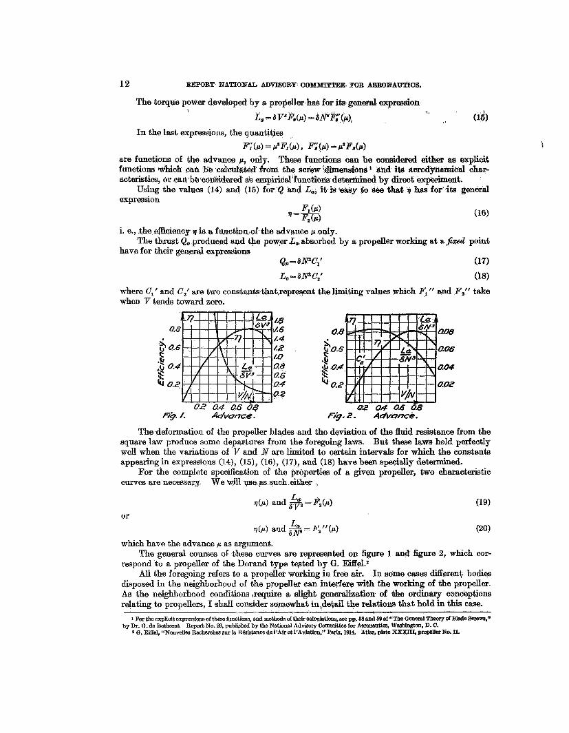
have for their general expressions The thrust Qo produced and the power Lo absorbed by a propeller working at a $xed point

& = bNaC,’ (17)

I;, = SP C;’ (18) where C, and 0,’ are two constanb th&repreqent the limiting values which Fl I’ and F,“ take when V tends toward zero.

E& L6 L 4

LO 0.8 Q6 a4 p.2

fig. 1. Advunce .

0.8

06 &

.c a4 04

* 0.6 .9,

8 0.2 02

@2 a4 ti& 0.8 Ftg. 2. Advunce .

The,deformation of the propeller blades and the deviation of the fluid resistance from the square law produce some departures from the foregoing laws. But these l a m hold perfectly well when the variations of V m d N are limited to certain intervals for which the constants appearing in expressions (14), (15)) (16)) (17), and (18) have been specially determind.

For the complete specihation of the properties of a given propeller, two characteristic curves are necessaq We will pa such.eitber ,

or

which have the advance p as argument. The general couraes af these ourves are represented on figure 1 and figure 2, which cor-

respond to a propeller of the Dorand type tepted by G. EiffeLa All the foregoing refers to a propeller working in free air. In some cases different bodies

disposed in the neighborhood of the propeller can interfere with the working of the propeller. As the neighborhood conditions mquira a, slight generalization of the ordinaiy conceptions relating to propellers, I shall consider somewhat in,detail the relations that hold in this case.

1 For the esplicit expressions of these functions, and methods of their calculatIons, see pp. 68 and 69 of “The General Theorg of BMe Smem,’’ by Dr. G. de Bothezat. Report No. 29, published by the Nation81 Advisory Committee for AemnaoticS, Wasbfngton. D. C.

0. Eiffel, “Nouvelles Recherche3 sur la RBsistance de 1’Air et 1’Aviation.” Park, 1914. Atlas, plate -1. propbr No. 11.

GENE'RBL .T&EORY OF' TSE' S@EL4DY fMOTIO'N IOF &l!T AIRPLAWEI. 13

Let US consider any vehicle of locomdtion;*ih om case hn ~+laneM$b@~&idm~'m angle ofattack'i and a speed V.' 'In*6rder,$o sbm tEe H&t of bheiakplane,i. e., to~o&ercomeIW fh'TMbthQce, it Ileceasw to. sixppl)r az$e.1.t&in d o h % of POW@, Whi& we W% IC& POW=

the vehik l~ . F~lr a g h n hhpl&e ~4th~ kv&aHe 10ad.i dt m t & d t i h d e r throttle kept at constant OF-, the power &rig a hcticin .ofi the fl$~@

y. This is because, as be seen later, the angle of attack i under such conditions function of the speed only. po$er L,, b delivered to the vehicle by a propulsor,

our case a screw blade propeller. It is self-evident that the power d e h e d h y tlp ~ C O - p+or to the vehicle is the same thing aa the pmm utilized by the vehicle. But in order to make the propulsor able to deliver the power to the vehicle, we must always deliver to the propulwr a ppwr La greateF than La, cgulled power absorbed by the p~opulsw-

It is the ratio

which we shall call the efficYency of khe pro@or It is easy to understand that the same ropul:or

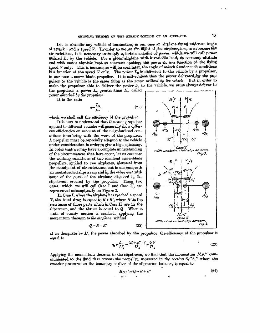
applied to different vehicles willgenerally s h d differ- ent eEciencies an account of the neighborhood con- ditions interfering with tho work of the propdqor. A propeller must be espwi&Uy adapted to the vehcle under consideratiion in order,to give a high effioiency. &I order that we may have t-t complete undeptwding of the circumstances that here occur, let us compare the working conditions of two identical wsew-blade propellers, applied to two airplanes, i&ntical from the standpoint of air resistame, but. in one, case, mth an unobstwcted slipstream and + the other awe with some of the parts of the airplane disposed ip the slipstream create? by the propeller. These two cases, which we will c+ Cye I and Case 11, are represented schematically on Figure 3,

In Case I, when the airplane has reached' a speed V, the total drag is equal to.R+R', where R'js tha, resistance of those parts which in Case I1 are in the slipstream, and the thrust is equal to Q. When a state of steady motion is reached, applying the momentum theorem to the airplune, w & h d

J IT"

&=R+R' (22)

Cose'T . with unobsfruc fed s//p Sfreom.

fiy. 3.

If we designate by LXa the power absorbed by the propulsor, thed€iciencg: 0% the propulsor 1s equal to t

' (23)

Applying the momentum theorem to the slipstre&n, we find that the momentum Mp," corn- municated to the fluid that crosses the propeller, measured in the section S,"S," where the exterior pressures on the boundary surface of the slipstream balance, is equal to

i&t+!'i=Q= R+R' (24) . a , > , t

14 lWPORT NATIONAL ADVISORY L!QBdll6P$TEE FOBr A I $ ~ ~ A a t I a s i

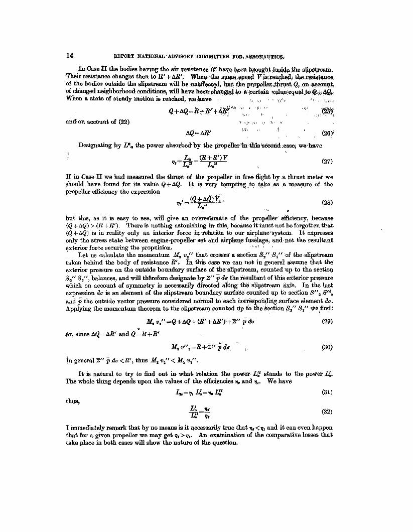
In Case I1 the bodies having the air mistance &< ham k e a bzjqqght ,jnpidp ,the %p$@am. Their resistance changes then to Zl'fbR', W h e ~ the s ~ . q w . ~ $ V jsrce@& tbe,rpisigwa of the bodies outside the slipstream will be unaffwtgd, Qqt the of changed neighborhood conditions, will have b m . c h @ d $0 ic?pert When a state of steady motion is reached, xehbaye

and on account of (22) ' ' " j ' t ~ i r I, 6s

Q + A Q = ~ + ~ +e?*" :iss+* :: ~a $ ' I < " L i yb9;

f

' (26)i rn ( I I AQ-L\R'

Designating by Lna the power absorbea by the propellbr' in *this 'S&m%d :casej w h ~ e

If in Case I1 we had measured the thrust of the propeller in free flight by a thrust meter we should have found for ita value &+A@. It i y very tempting?to take as a mgagure of the propeller e6ciency the expression

(2%)

but thm, as it is easy to see, will give an overestimate of the propeller eEciency, because (Q +AQ) > (R + R'), There is nothing astonishing in this, bechusd itmust not be forgotten that (Q +A&) is in reality only an intenor force in relaticin %to om airplarreqwtem. It expresses only the stress state between engine-propeller seb and &irplaqe fuselage, and. not the resultant

Let us calculate the momentum &fa vat' that crosses a section fi2" S," of the slipstream taken behind the body of resistance R'J In this case we can not in general assume that the exterior pressure on the outside boundary surface of the slipstmam, counted up to the section $ 2 f f 8,") balances, and will therefore designate by 2" 11 do the rbultant of this exterior preaure which on account of symmetry is necessarily directed along tWe slipstream In the last expression do is an element of the slipstream boundary s u r b e ctmited up to section S", S", and $ the outside vector pressure considered normal to each bor$%pondixig surface element da. Applying the momentum theorem to the slipstream counted up to the section S," S," we h d !

+AQ)Va 7s - + a

gxterior force securing the propulsion. 1 . I . s

8

In general Z" 5 do <R', thus N, v," < M, vl'. It is natural to try to find out in what relation the power Lil stands to the power L:.

(31)

(321

The whole thmg depends upon the values of the efficiencies qs and ql.

thus,

We have

La = q1 4%: = r], Lf

I immediately remark that by no means is it necessarily true that qs <ql and it can even happen that for a given propeller we may get qs> ql. An examination of the comparative losses that take place in both cases will show the nature of the question.

where: I

Mi =fluid mass that crosses the propeller disk in a unit of time. v:=slip velocity in section SY '* I;' =moment of inertia of the fluid mass .MI in rseOtion if?;' &: 0;' =race rotation in section 8;' s;' vi -slip velocity in the plane of propsller:rotg$oq., C, = torque acting on the ,propeller axis. w, +=race rotation in the plane of the propeller.

I

1

The flow conditions in the slipstream are assumed uniforfn for sakb of simpfitiky. On the other hand we have,

Lt=Ci $=Q(V+Vi )+4 wi+j$

where

62, = angular velocity of propeller rotation. pf =losses by impact and friction of the flmd against the propeller blades.

We thus finally find

and .Et; = VQ +'I$ Mi v;', + I;' w;" t! p f '

Applymg in Case I1 the theorem of kinetic energy, me find

Ms ( V+V~)*+'/~ I: w;--*/# .& V"-K( V + V ~ ) (p0-@)+'(&+A,&) ( V+V~J+G, we- (R'+AR') ( V+W~>

or since Q t AQ= M, v; t (R' +AR') - X' p du and considering 2; p de&; (pD-p'') where Si TS the area of the section Si Si of the slipstream, po the outside pressure, and p i Lkie pressure in section Si 8; we get.

(Q t AQ) (v-cv,) + c, wg= V(Q+ AQ) + I / # M, V: +itz zz: wi8 - x;(p0 - p ; ) ~ ; + (R'+AR')v; (37)

where M,, vi) Zi) a:, C,, W, have meanings analogous to Case I, Si (V + wy) (po - p i ) represents the work of the resultant exterior pressure rom the work of the pressures in a section far in front of the popkdler and 'm section .e Ti, where po m d pz ar0 the corresponding pressures ) ( V + vi), a mean velocity included between ( V + VJ and C'Vt-.t$) whose product by (R' t AR') represents the work corresponding to that resistance.

p dk considered as built

But as:

Gr = Cs s2,= (Q + AQ) (V +vJ + cs u s + pf' (38)

(with 62, and pf' having meanings analogous to Case I) we finally find.

.L?= V (&+A&) + I / # M , Vz+'/, 1; (P0-p:) V i + (4' +&I) or, AQ=ARf

Lf=VQ+' / , M8v:8+i/s Z ; w ~ + r l ' ~ i + A R ' ( V + V ~ ) 2% (Bo-$) JU;+~:' (39 1

16 REPORT NATIONAL ADVISOBY OOMMITTEE FOR BEftONA?T‘ZIrnb

and

For the ratio of Li to Lfi’ we find the value .

In general (C; wI + p f ) and (Ca but generally Va <v,.

are of the same order of magnitude; (&+A&)>&, > We thus can nat decide a priori between V, =(

I would warn those who think tha% the losrJes [R vi + LW(V +vi)] can be estimated eady. As a matter of fact First, the velocity in the slipst$eam, when some bodies are introduced into it, is totally changed in comparison with h free slipstre8;m: second, bhe Slipstream is not a uni-

with free boundaries, the formulae and coeEcients of “fluid resistance deduced from experiments in fluids of infinite boundaries can not be applied to it, especially when the bodies considered do not have small cross sections in comparison with the cross section of the slipstream.

The efficiency 7, will be called propkive egicieney and designated by qP. We shall designate by f, and call it neighborhood factor, the ratio of the propulsive esciency to the free efficiency

form current, but a current of variable velocity gong its +s, third, as the slipstream is a stream I

The efficiency rl, will be called free e-, and designated in the following by 7,.

We thus write 7,=f?Jr (42)

It is understood that the neighborhood factor f can be

A3 has been mentioned already, the free efficiency qf is a function of the advance p= V/N only But as the slipstream created by a given propeller is also a function of p only, the neigh- borhood factor, for a given propeller and given neighborhood conditions, can be a function of 1.1 only. !l%w the prophive e$cienq must 6e a function of the advance 1.1 mly.

In airpkne testing, it is the propulsive e#cien y qp that has to 6e measured in order to evaluate the propeller in the actual working conditim.

One could raise the following two questions.. a. In what relation does the thrust (Q+AQ) of Case I1 stand to the momentum H,, vi in

section S a 8; (see Sg. 3) a It is easy to see that

Q + A& = HB vi+ 2’ $u

w b m Z’ jidv is the resultant of the outside pressure pn the whole b o u n d 9 of the slipstream counted up to the section 8; 8;. Between .the momentum Ne vi and Ma vi we have the relation :

illa v6’t (R -FAR‘) - 2’’ pa@= &is vi+ r, pda 6. What would the momentum in section Si S’ be if th0 whole resistance R+R1 had

beep put in the slipstreamS It is easy to see from relation (30) that we simply have:

M~ = Z” pav because the resistance left outside the slipstream is in this case equal to zero.

efficiency This would carry us too fa r into the RrQpeller theory I shall not go into a more detailed study of this importmt questioa of the propulsive

Those who would like to ‘For experimental data referring to the slrpstrasm efpect 8e8 “The design of screw propellers,” London, 1920, pp. 192-196, by Henry C. Watts.

GENERAL THEORY OF THE STEADY MOTION OF AN AIRPLANE. 18 have a deeper understanding of the foregoing discussion are refemd to the author's ccChneral Theory of Blade Screws," previously mentioned.

B. pBOpEBTIE8 OF TEE ENGINE.

Many discussions have been brought about by the ques e p w y L, of a given gasoline engine, as actually used on airplanes, Such discussions are rather a misunderstanding, because the power L, does not depend on the altitude, but depends only upon:

1. The number of revolutions N at which the engine is running. 2. The throttle opening x. 3. The density 6 and temperature T of the air in which the engine is working. 4. The quality of the gasolie used. The question &s to how density and'temperature are connected with altitude depends

exclusively upon meteorological conditions, which as known, ariable through the day, as well as through the year. tKe standard atmosphere will be discussed briefly.

Since for a given mass of air, its pressure p, density 6 and absolute temperature T are connected by the Claperyon relation p/6 = gR Twhere R is the gas constant, the brake horsepower can be as well considered as a function of the pressure p and temperature T. But since the propeller thrust and the forces of air resistance depend on the density 6, it is more. convenient to relate the power L, directly to the density 6.

In the following chapter the ques

300

c sB2m & p /OD

' 300 9012 /SUU ?/@ f f g . 4. R. P. M. Fig. 6. R. I? M.

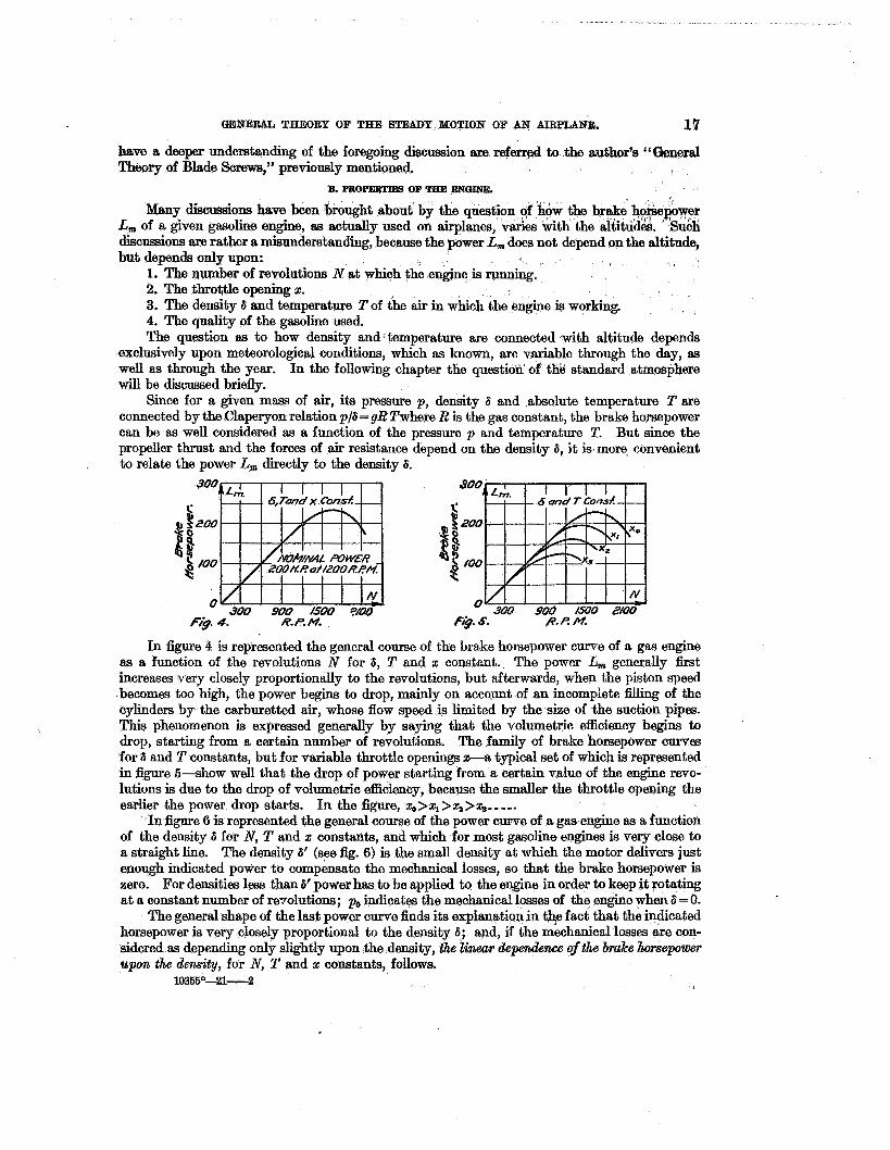
In figure 4 is represented the general course of the brake horsepower curve of a gas engine as a function of the revolutions N for 6, T and x constant. The power L, generally h t increases very closely proportionally to the revolutions, but afterwards, when the piston speed becomes too high, the power begins to drop, mainly on account of an incomplete slling of the cylinders by the carburetted air, whose flow speed is limited by the size of the suction pipes. This phenomenon is expressed generally by saying that the volumetric efficiency b e g h to drop, starting from a certain number of revolutions. The family of brake horsepower curves for 6 and T constants, but for variable throttle openings x-a typical set of which is represented in m e 5-show well that the drop of power starting from a certain value of the engine revo- lutions is due to the drop of volumetric efficiency, because the smaller the throttle opening the earlier the power drop starts. In the figure, % > x I > ~ > % - - - - .

In figure 6 is represented the general course of the power curve of a gas engine as a function of the density 6 for N, T and x constants, and which for most gasoline engines is very close to a straight line. The density 6' (see fig. 6) is the small density at which the motor delivers just enough indicated power to compensate the mechanical losses, so that the brake horsepower is zero. For densities less than 6' power has to be applied to the engine in order to keep it rotating at a constant number of reyolutions; p,, indicates the mechanical losses of the engine when 6 = 0.

The general shape of the last power curve finds its explanation in the fact that the in+cated horsepower is very closely proportional to the density 6; and, if the mechanical losses axe con- sidered as depending only slightly upon the density, the l&war depmdence of the bmke horsepower upon the density, for N, T and x constants, follows.

10355°-21-2

" . ,

4.8 REPORT NATIONAL ADVISORY COMMITTEE FOR AE&ONAUTIO&

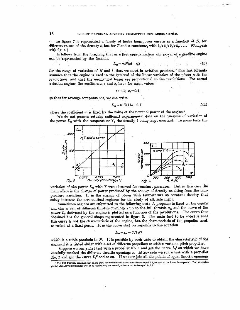
In figure 7 is represented a family of brake horsepower curves as a function of N, fm (Comp&re different values of the density 6, but for T and x constants, with 6, > 6, > 6, > 6, - - - -.

with fig. 5 . ) It follows from the foregoing that as a fmt approximation the power of

can be represented by the formula L, = mN(& - 6) + (43)

for the range of variation of N and 6 that we meet in aviation practice. This la& formula assumes that the engine is used in the interval of the linear variation of revolutions, and that the mechanical losses are proportional to the aviation engines the coefficients c and c,, have for mean values

c = l l ; co=o.l

so that for average computations, we can write

L,=rnf l ( i l~- - 0.1) (44)

where the coefficient m is fixed by the value of the nominal power of the engine.'

the power L, with the temperature T , the density 6 being kept constant. We do not possess actually suflicient experimental data on the question of variation of

In some tests the

0.025 0.075 W25 900 900 I500 2lm tig. 6. Dendfy (&wfon/~') ftg. 7. R. p. M.

variation of the power L, with T was observed for constant pressures. But in this case the main effect is the change of power produced'by the change of density resulting from the tem- perature variation. It is the change of power with temperature a t constant density that solely interests the aeronautical engineer for the study of altitude flight.

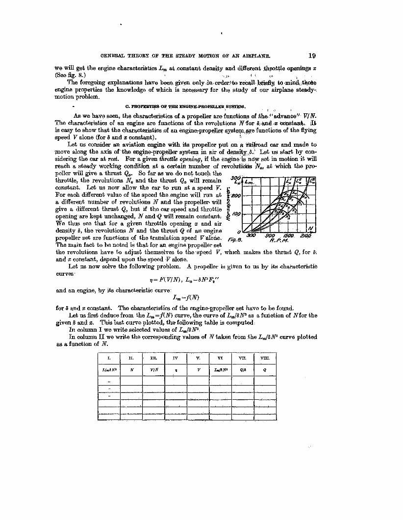
Sometimes engines are submitted to the following test: A propeller is fixed on the engine and this is run at Merent throttle openings x up to the ful l throttle 4, and the curve of the power Lo delivered by the engine is plotted as a function of the revolutions. The curve thus , obtained has the general shape represented in Sgure 8. The main fact to be noted is that this curve is not the characteristic of the engine, but the characteristic of the propeller used, as tested at a fixed point. It is the curve that corresponds to the equation

which is a cu3ic parabola in N. engine if it is tessed either with a set of different propellers or with a variablepitch propeller.

carefully marked the different throttle openings 2. No. 2 and get the curve Lou and so on.

It is possible by such tests to obtain the characteristic of the

Suppose we run a fh t test with a propeller No. 1 and get the curve L,' on which we have Afterwards we run a test with a propeller

If we now join all the points of equal throttle openings 4 The last formula ~ssumes that at sea level the mechanical losses constitute around 7.5 per cent of the brake horsepower. For an cmgine

giving at ma level 200 horsepower, at 25 revolutions per second, m turns out to he equal to 6.2.

GENERAL THEORE OF TBE? STEBDY MOTION OF AR bEPLBETE. 18

we wiU get the engine charaeterihtics L, at constsnt densify and Herent $hpottla openbgs x

to min&:tl@ie i ' (Seek. 8.) 1 t t 1 I f

The foregoing explanations hme been given b d y in.order3t.o reo engine properties the knowledge of which is necessary for the study of our airplane steady- motion probled.

C. PRQPEiZTIES OF THE ENGBNE-PBOPELLEB,SYSTEM. 1 '

As we have seen, the characteristics of a propeller a m functions of &he VI The characteristics of an engine are functions of the revolutions N Yor s.itu~d 1: ooWm&. is easy to show that the characteristics of an engine-propefier systcqqwe functions of the flying

Let us consider an aviation engine with its propeller put on fi r&&oad car and made to speed 'ir alone (for 6 and 1: constant). h

move along the axis of the engbe-propller system in air of sidering the car at rest. For a given throttle opening, if the reach a steady working condition at a certain number of peller will give a thrust Qo. So far as we do not touch the throttle, the revolutions No and the thrust Qo will remain constant. Let us now allow the car to run at a speed V. For eaoh different value of the speed the engine will a different number of revolutions N and the propeller! give a different thrust Q, but if the car speed and throttl opening are kept unchanged, N and Q will remain constant+. We thus see that for a given throttle opening 2 and air density 6 , the revolutions N and the thrtlsfi @ of an 'engine

The main fact to be noted is that for an engine propeller set the revolutions have to adjust themselves to the speed V, which makes the thrust Q, for 6: and x constant, depend upon the speed 3V alone.

Let us now solve the following problem. A propeller is given to us by its characte9lstic curves

and an engine, by its characteristic curve

for 6 and x constant. The characteristics of the engine-popeller set have to be found.

given 6 and 2. This last curve plotted, thefollowing table is computed

'2:

0 propeller set are functions of the translation speed V &lone. ~ 9 . 8 . R. t? M.

q = F(V,TIN), L,,=SPFz"

L,=f(N)

Let us first deduce from the L, =f(N) curve, the curve of Lm/SNs as a function of Nfor the

In column I we write selected values of LmfGNs. In column I1 we write the corresponding values of N taken from the Lm/GNs curve plotted

as a function of N .

20 REPORT NATIONAL ADVISORY COMMf”EB ’FOR AERONAUTIC^.

When a propeller is &ed to a given dnginei the power absorbed by the propeller is to the power delivered by the engine and both run at the same number of revolutions (h 6 ~ 8 of gearing, the g&dg constant haS.only to be introduced) that is, we hwe

Lm - La S N s - s l V s

1

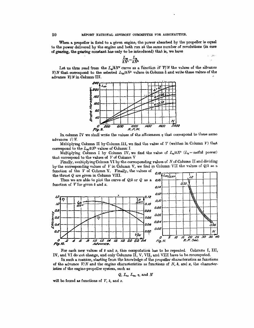
&Let u9 thus read from the La/dN* curve as a fhction Gf ‘V/N the values of the ai-lvance V,N that mmespoad to the selected Lm/&W values .in 0oZumn~I.and write these values of the advrknm V/N in C O l ~ n1. I

9. A. P. M.

In column IV we shall write the values of the efficiencies 1) that correapond to these same advances VlTI2y.

Mfdtiplying Column I1 by Column 111, we h d the value of V (written in Column V ) that correspond to the L,/6Ns values of Column I

Multiplying Column I by Column IV, we h d the value of L,16Ns (&%=useful power) that correspond to the values of V of Column V

Finally, multiplying Column VI by the corresponding mlues of N of Column I1 and dividing by the corresponding values of V in Column V, we flnd in Column VI1 the valves of &/a as a function of the V of Column V. Finally, the values of the thrust Q are given in Column VIII.

Thus we are able to plot the curve of Q/6 or Q as a a16 function of V for given 6 and 2.

fig. [I. R.P. Sec. f& 10. Advzmce.

For each new values of 6 and x, $his computation has to be repeated, Columns I, 111, IV, and VI do,Izot change, and only Columns 11, V, VI?, and VI11 have to be recomputed.

In such a manner,.starting from the knowledge of the propeller characterlstics as functions of the advance VIN and the engine characteristics as functions of iV, 6, and z, the chaxacter- istics of the engine-propeller system, such as

wil l be found as functions of V, 6, and x. Q, Lw Lm, N

GENERAL THEORY OF THE STEADY MOTION OF AN AIRPLANE. 21

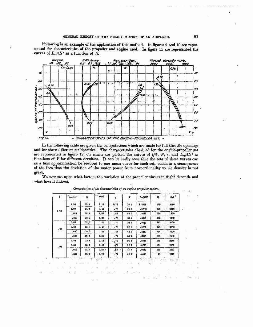
Following is an example of the application of this method. In @pres 9 and 10 me repre- sented the characteristia of the propeller and engine used. In 6 p e 11 are represented the curves of Lm/SN3 as a function of N.

In the following table are given the,computations which are made for full throttle openings and for three Merent air densities. The characteristics o b t h e d for the engine-propeller set are represented in figure 12, on which am plotted the curves of &/6, N , q, and Lm/SN3 as funotions of V for different densities. It can be easily seen that the sets of these curves can as a b t approximation be redubd to one mean curve for each set, which is a consequence of the fact that the deviation of the motor power from proportionality to air density is not great.

We now see upon what factors the variation of the propeller thrust in flight depends and what laws it follows.

Computation of the charmte&sties of an engine-propellm system.

REPORT Nq. ?'Iw PABT JII.

THE AT1\IOSPHEBE.

1. Sam GENERAL PROPERTIES OF THE ATMOSPHERE.

A short review of those properties of the atmosphere that have a direct relation bo tk

The specific weight of air-expressed in Idldgrams-will be represented by u. The density of air-expressed in newtons will be represented by 6. We have b

At the pressure of 1 atmosphere=10330 klg/mt2 and absolute temperature T= 273' + 1 5 O =

airplane steady motion will be given here.

u = g6 with g = 9, 81mtlsee2

288O, the specifio weight and density of air have for mean values

u=1,225 klg, 6=0,128 newton.

At the same pressure of 1 atmosphere and zero degrees centigrade (T=273) we find

u,=1,293 klg; 6,=0,132 newton.

Using the former values, the gas constant R, deduced from Clapeyron's relation

p=vRT (45) has for its value

R = 2 = 10330 -29,27 UT 1,225 X 288- (46)

,Let US consider the atmosphere to be in a perfect static condition (no winds) If we rise in such an atmosphere through a distance dH, the pressure p will vary by an amount 4 2 , equal to

or on account of (45) - dp UdH (47)

(If in this last formula we consider dplp = 0.01, R = 29,27, T- 273 we find dHZZ80 mt. This means that a difference of pressure of 1 per cent in the atmosphere corresponds at Oo centigrade to a change of altitude of 80 mt.)

Integrating (48) we get

(49)

where p o is the preysure at the altitude H, and H> H,,. This last formula gives the value of the altitude H from the knowledge of pressure, when the law of variation of the temperature T With altitude is known, For T=273; p/p0%3.5 and H,=O, we find 8 ~ ~ 5 , 0 0 0 mt. In an isothermic atmosphere of zero degrees centigrade, at the altitude of around 5000 mt the pressure is one- half of the ground level pressme.

,,=,[dH - T

22

GENERAL THEORY OF THE STEADY NOTION OF AH AIRPLANE. 23

2. DISCUSSION OF THE STAJSDABD ATMOSPHEIW.

This question of the law of variation of temperature with altitude has been late19 a matter of considerable discussion. Numerous so-called standard atmospheres have been pkopos which are supposed to be some kind of average deduced from Merent sets of meteorolo observations. The Paris “Peace Conference of 1919” has even considered it necesiiraxy to f& by interallied agreement, some kind of standard atmosphere.

A careful examination of all the propositions mad6 has brought me to the conclusion that this question of the standard atmosphere has been somewhat misunderstood.

Let us consider the whole question from a general standpoint and make clear for what purpose we need the standard atmosphere in aviation.

For eacli geographical position, a t a given hour of a given hay, there exists along the verticd drawn through the place considered, a certain distribution of pressures ’and temperatures. This distribution of pressures and temperatures depends upon the meteorological conditions and is variable through the whole year. The variations of this pressure and temperature are very important. It is well known that the same pressures and temperatures can be met at levels where altitude differences can amount t o several thousands of meters. If a certain mean distribution of pressures and temperatures is adopted, the deviation from this mean distribu- tion can also make up actual altitude differences of the order of a thousand meters.

On the other hand for an airplane, the forces of air-resistance, the propeller thrust, and the power of its engine are all functions of the air density and decrease with this. It is a property of the airplane to be able to reach a certain limiting small value of the air density, at which the airplane can still %y level, but is unable to climb any more. This limit of density is called the ceiling density 6,. The aviation engineering problem consists in finding for each airplane its ceiling density. But the question, at what altitude this density 6, is located is purely a meteo- rological question. The distribution of densities in the air is greatly merent and the same den- sity can be met on different days at very Merent altitudes. The question of the relation of densities and altitudes stand outside the aviation engineering problem and is merely a question of public c6riosity. Technically speaking, we can only say that a given airplane has the ability to reach a certain density 6,. The smaller this density 6,, the greater is the climbing capacity of the airplane considered. There is no reason for exprossing this density in altitude figures, because density already completely specifies the question. There is only one fact that must still be taken into account. The power of the airplane engine, at a given density, depends somewhat upon the temperature. When w0 speak of airplane performances, they must thus be referred to a certain temperature. In the selection of this temperature, we must be guided only by convenience and simplicity. There are no reasons to adopt a temperature variable with the altitude, but there are many reasons for adopting a constant temperature at all altitudes.

It is easy to see that, exactly speaking, it is rather standard conditions for engine work that we have to select than to adopt a standard atmosphere. If we make the temperature variable with altitude, in other words, with density, this would mean that the standard con- ditions adopted for engine work consist of a special temperature for each deniity. This introduces a very troublesome element in engine-power computations, which is neither neces- sary nor demanded by any reason. On the contrary, a constant temperature for all densities is a natural condition, demanded for the sake of simplicity of the standard conditions adopted.

We are thus brought to the conclusion that from the standpoint of aviation engineering the only standard atmosphere that can be reasonably adopted is the isothemic atmosphere.

The p o p o s i h n of the author is to adopt for aviation enqheering, as a s t a d r d ’ atnwsphe, an atmosphere of constant temperature in its whole mass equal to zero degrees centigrade.

The advantages of mch a convention are as follow: 1. In all questions of design and performance prediction all temperature corrections are

totally eliminated. 2. In airplane testing the only correction to be made is the temperature correction of the

engine power and reduction of the performance to this corrected power. This correction is

.

+

24 REPORT NATIONAL ADVISORY COaMITTEE FOR AERONAUTICS.

quite simple, since we reduce each of the quantities to the same temperature independent of the altitude.

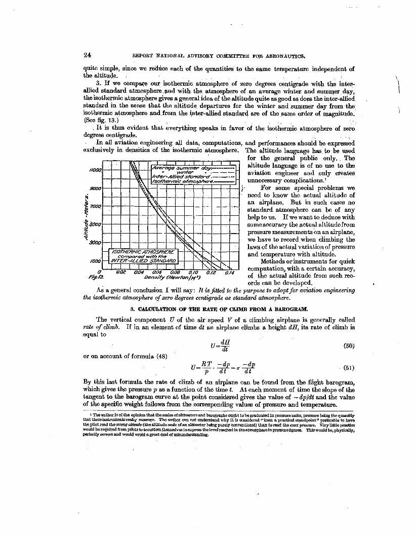
3. If we compare our isothermic atmosphere of zero degrees centigrde with the inter- d i e d standard atmosphere and with the atmosphere of an average winter and summer day, the isothermic atmosphere gives &general idea of the altitude quite &s good 8s does the inter-allied standard in the sense that the altitude departures for the winter and summer day from the isothermic atmosphere and from the ipter-died standard are of the same arder of magnitrude. (Seek. 13.)

It is thus evident that everything speaks in favor of the isothermic atmosphere of zero degrees centigrade.

In all aviation engineering all data, computations, and performqnces should be expressed exclusively in densities of the isothermic atmosphere. The altitude language has to be used

for the general public only. The altitude language is of no use to the aviation engineer and only creates unnecessary complications.’

For some special problems we need to know the actual altitude of an airplane. But in such cases no standard atmosphere can be of any help to us. If we want to deduce with some accuracy the actual altitude from pressure measurements on an airplane, we have to record when climbing the laws of the actual variation of pressure and temperature with altitude.

Methods or instruments for quick computation, with a certain accuracy, of the actual altitude from such rec- ords can be developed. I

Ar; a general conclusion I will say: It isJitted to the pwrpose to adoptfor aviation engineering

/1000 .-.---

2 f: 8 SUUO 3

3doO

$ 7uou

3

D Densify fNewfan/Ma)

the isothemic atmosphere of zero degrees centigrade as standard atmosphere.

3. CALCULATION OF THE RATE OF CLIMB FBOM A BAROGRAM.

The vertical component 17 of the air speed V of a climbing airplane is generally called If in an element of time dt an airplane climbs a height dH, its rate of climb is rate of climb.

equal to

or on account of formula (48)

By this last formula the rate of climb of an airplane can be found from the a g h t barogram, which gives the pressure p as a function of the time t. At each moment of time the slope of the tangent to the barogram curve at the pbint considered gives the value of -dp/dt and the value of the specific weight follows from the corresponding valum of pressure and temperature.

1 The author is of the opinion that the scales of altimeter8 and barographs ought to be graduated in prassureunits, pressure being the quautiw that theseinstrumentsrd$ measure. The author mn Mt understand why it is considered “from a practical standpoint” prefemble to have the pilot rend the wrong alti*rde (the altitude scale of 8n altimeter Mng purely conventional) than to read the emu pressure. VCq little practice mould berequired frompilots toaccustom themselves toexpress thelevelreachadin theatmmphereinpmsureflgmw. This wouldbe,physieally, perfectly m e e t and mould avoid a great deal of misunderstanding.

GENEBAL THEORY OF THE STEADY MOTION OF AN AIRPLANE. 25

4. INFLUENCE OF WINDS AND SELF-SPEED ON COCKPIT PRESSURE-

Let us consider briefly what influence the atmospheric winds can have on the observed Consider two air masses at nearly the same altitude, in which the Bernouilli constant

having a speed of 10 meters per such conditions that the pressures

pressures. has the same value, one mass havin second which is itself a strong &,e

in them two air masses are related by the eqpqon

k

or -a

At gound level witk p l = 10330 iElg/mF this &;ties

6 25 pzlp, = 1 - eo = 0, 9994

The differefice between p , and p , thus appears to 6e of the order of 0.05% of the atmosphe+c pressure, which corresponds at ground level to a difference of altitude of around 4 meters. At an altitude where the pressure wodd be 10330/2 (@round 5,000 meters) the difference between p , and p , would be double and this would still correspand ~ n l y to a difference of altitude of 8 meters. We are thus brought to the conclusion that ordinary winds will &ect.only slightly the calculation of altitude from pressure distribution.

A much more marked inaucnce i s that,of the variation of the airplane speed V upon the measurements of pressures as made on an airplane. The difference between the static pressure p at the level where the airplane is flying and the pressure p' in the cockpit is Tery closely equal to

An airplane in climbing can have its speed reduced to about half of iks hbrhontal self- speed, that would give for the cockpit pressures p', and p', corresponding to the two cases, a difference of

6 VZ p,' - p,'=O, 7 5 2

This is the difference between the "corrections" which are necessary in the two cases in order to determine, from the cockpit readings, the real ststic pressures. With Vg50 meters per second, at ground level, this can be about 1% of the atmospheric pressure, or 80 meters difference in altitude. Such differences have to be taken into account when pressure observations are made in the cockpit, at different values of the speed. The last circumstance may make it desirable to use special devices allowing the direct observation in the airplane of the static pressure, instead of the cockpit pressure.

REPORT No. 97. PA&T IV.

THE THEORY OF STEADY MOTION.

1. THE BASIC EQUATIONS. 8

All of the properties of the airplane steady motion are a direct consequence of the fact that

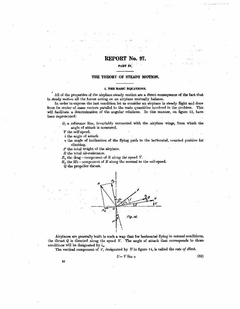
I n order to express the last condition let us consider an airplane in steady fiight and draw This

In this manner, on *e 13, have

Gf a reference line, invariably connected with the airplane whgs, from which the

V the self-speed. i the angle of attack. y the angle of inclination of the flying path to the horizontal, counted positive for

P the total weight of the airplane. R the total air-resistance.

in steady motion all the forces acting on an airplane mutually balance.

from its center of mass vectors pardel to the main quantities involved in the problem. w i l l facilitate a determination of the angular relations. been represented:

angle of attack is measured.

climbing.

Rz the drag - component of R along the speed V. R,, the lift-component of R along the normal to the self-speed.

Q the propeller thrust.

V

U -

i ’ Airplanes are generally built in such a way that for horizontd flying in normal conditions,

The angle of attack that corresponds to those the thrust Q is directed along the speed V. conditions will be designated by io.

The vertical component of V, designated by U in figure 14, is called the d e of dimb.

U = V S i y 26

. *

GENERAL TECEOBY OF THE STEADY MOTION OF A H BIRpLB1pE. 211

Let us now project all the form acting on the airplane on the direction of the speed V and the normal to it. The conditions of steady motion w i l l then be expressed by

(53)

(54)

9 , 1 Rx=Q Cos ( i - iJ -P Sin y

R,=P cos y-& sin (i-iJ

in which equations, we have:

R,=kx 6 A P (55)

R,=k, 6 AV' (56) where

7Ez = drag coeffioient. k, =lift coefficient.

6 = air density at flying level. A = area of the airplanq wings.

To these two equations (53) and (54) must be added the fundamental relation that connects the engine with the propeller.

L, (x, 6, N)=La=6N3 T," - (57) (3 which expresses the fact that in steady flight the power L,,, delivered by the engine-a function of X, 6 and N-ia always equal to the power L, absorbed by the propeller-a function of N, 6 and VjN.

The detailed discussion of the fundamental equations (53) and (54) is greatly complicated by the complex laws, fixed by the relation (57) governing the variation of the thrust Q in %ht, which we have considered in ful l detail in the foregoing.

In order to allow a better survey of fundamental properties of the airplane in steady motion, without complicating the question by those factors that have only a slight influence on the quantitative value of the results and do not affect a t all their general meaning, we shall make the following simplifications in equations (53) and (54).

I shall first remark that, on the one hand, we do not possess any reliable information as to the laws of variation of the propeller thrust for the case when the sehpeed B makes a certain angle with the propeller axis, and on the other hand, since the angle (i-io), as we shall see later, can take only small vdues in normal flying conditiona, we ahall consider it to be a su€Ecient approximation to assume

Q Cos (i:i,,)=Q Q Xi% (i - i o ) r O

It must be further noted, that in normal flying conditions, the angle of the flying path to the horizontal does not usually take large values. It seldom exceeds 15O, taking larger values only in steep, dives and steep glides, which must be considered separately. W e thus assume

b'in ysy; Cos y ~ l .

Introducing these simplifications in the equations (53) and (54) we get:

* R,4* 6 A P - Q - P y (58)

R,=k, 6 A P = P

The simplifications we have made affect principally the value of the self-speed V, which we shall calculate from the equation V - d P m instead of the more exact relation V= 46'0s ?7/P/k, 6 A. But it is easy to aee that for y < 5O we have 6'0s y > 0,96 and the error made in the speed will be less than 1 - &%z&, 02, that is less than 2 per cent. In any case,

28 REPORT: NATIONAL dllvIsoRp OOMMITTEB FOE AERONAUTICS.

when necessary, once the selfi9peed~~~Qbtained by equation 459) and the value of 7 known, it is always possible to correct its valuiz by t

For the study of the airplane in steady motion, it i s wore convenient to consider, instead of the relations (58) and (591, the system of equations

it.eqUa1 to Y

+.& ~ k x P ky

which follow directlv from the last. With the same "approximation, the rate of climb 157 has for its vdue

U = V r (62)

It is from the system of equations (60) and (61) that we sh$l dedum all the properties of an airpl'ane in steady motion. Once all of the mutud intprrelations of qll the quantitiesinvolved in the problem are perfectly established, all quantitative corrections, when demanded, can always be made post factum and in our state- ment of the problem, are ody necessary in the case of steep climb% or glidihg

We shall start by the study of the steady motion of an airplane of COR- stant total load weight P and constant wing area A, the engine working all the t h e at full throttle opening.

For this study we shall make u88 of a graphical interpretation of the equa-

and (61) which comists of the

'

2. THE B$ETEOI).

The lift coefficient kv will be adopted as fundamental variable. As

the lift coefficient k,, is a function of the angle of attack only, under the restrictions made, its value can be changed in flight only by a displacement of the control stick.

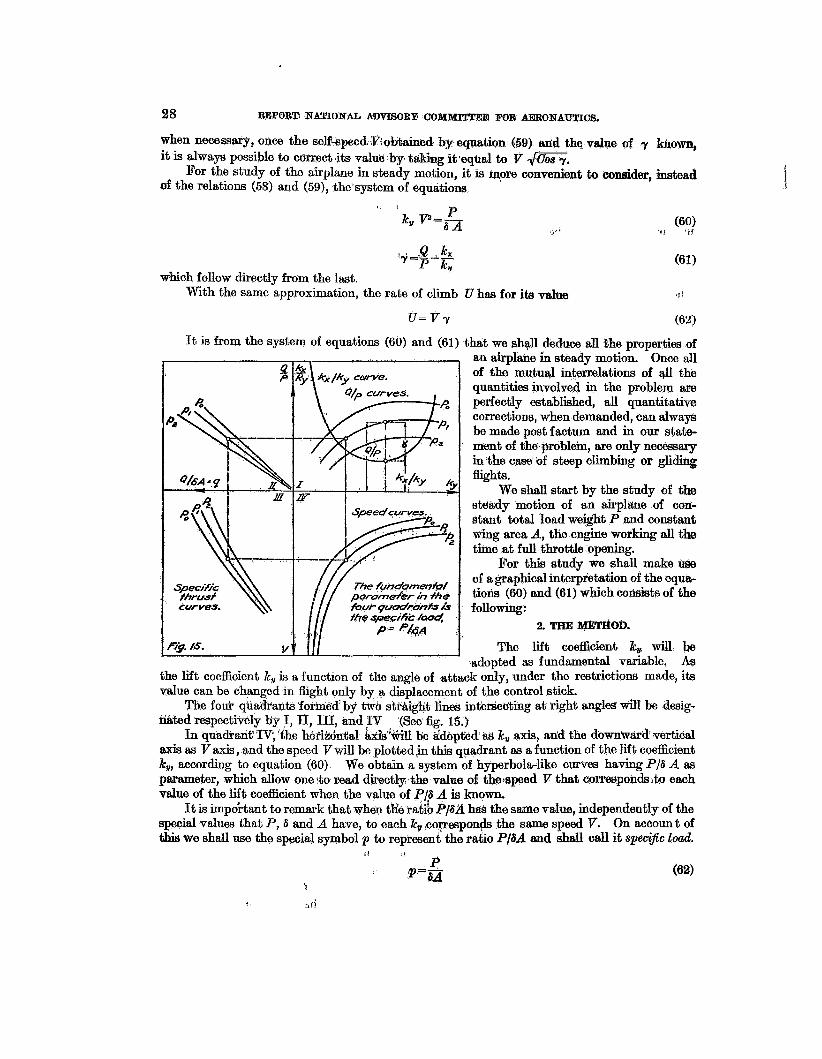
The fouk quadrants formgd' by tw& str&ight lines intersec'ting at right angles will be desig-

+iAcin%al $xi4't+iU be ddbpted as k,) axis, and the downwmd vertical ra;xiS as V axis, and the speed Vwill be plotted,in this quadrant as a function of the lift coefficient 4, according to equation (60) We obtain a system of hyperbola-like curves having PI6 A as parameter, which allow one tto zead diwictl,, the value of theaspeed Y that corresponds to each value of the lift coefficient when the value of PIS A is known.

It IS impo?tant to remark that when tge ratif0 PI82 has the same value, independently of the special values that P, 6 and A have, to each kv poFesponds the same speed v. On account of this we shall use the special symbol p to represent the ratio P/SA and shall dl it speci$c load.

I, 111, and I V (See fig. 16.)

i

P Pp'a

29

It will be seen from aU that folk&& that the spec& 10Sd p is @e fundamenttal~pammeter of &the whole problem of $mdy.motion, I 24

The curves of V as a function of kv with easy to sea tbt &he speed ourves-in, the a mathematical relation independent of bhd4,sp famiy of speed curvea co~p6n&S; t~ any r&$meJ. *ThpIast prop&@ of the ~pmd~cmizis is a coDsequence of our selection bound level) pa,qs- - _ _ is s propeller aptem, $bat the thrust Q function of the spe& V and density sake of uniformity, we shall consider,

We have awn,. w h

cal1,spepeci;fie thrust .and designah by p, i. e.,$ I

It is easy to see that the'speclfio' 'thrust ~~ISO'BB, 16i.4 ddnstttnt df the sped V and density 6 , orl in othdr Flior&, a'fimtjtiofi df B and as P and A are constants of the a i r p h e considered. 'We bhiiIr pro6 id qudrdnt I11 the curves of the specific thrust p = P/6A as a fimction of' the &elf2qbd Y 6 t h 'the bpecific lbad p = P/sA as parameter, the horizontal axis being the q h S i . spcific thrust curves is repre-

IV. We have learned in previous chapters how t this family of curves from the properties of the propeller and engine wed on the; airplane considered. The specific load curves auOw us to deduce directly the value of the propeller thrust that corresponds to each flying speed.

Knowing the laws of vmiation of the thrust Q as$& function of the speed V, it is easy to deduce the laws of variation of the thrust Q asc a function of the .lift coefficient k,,. FOE this purpose, let us consider the equation

(64)

sa ted in figure 15, with the parameter p having the ues pol pi1 pa in quadrant

and interpret it as a family of straight lines pwing through the origin with p as abscissa, y, as ordinate, and p as parameter, and plot these straight lines in quadrant I1 of figure 15, givmg successively to p the Val- po, p , pa-- ahd using thcherticttl axis as the y =Q/P &. We shall call these last lines trader 1i.neS.

This system of transfer lines once plotted in quadrant 11, it is easy to trace directly in quadrant I, for each given value of the specific load p, the curve of the ratio QIP as a function of k,, that corresponds to a given curve of q=Q/6A as a function of V Each two corresponding points of two copeaponding cum@ o diagonal verticm of a rectangle whose sides are par@$ to icq.3 are located one on

ant 11, corresponding to the,s<yqe value o$ the sp can deduce, @ quadrant I, from the specific thrust a function of kw with p as parameter, which give us t& of t&q lift; c$oe&cient. A set of such curves of Q/P & e values po, p l , p2 - of thespecific load, is represented in quadrant I of @e,a5. We new w that the chart represented on this %&re has the property that each f m p m m p d h g in the four q d r & I , II, III and IV lie on the vertices o f a r a y & ? with its +,gar&! to the a m .

Let IS fhially'plot in quadrht I, ih addition to tli8'Q$(P s"& a f'unct5on of E,,, the curve of the drag-lift ratio kJk, as a functioq, of& A s the drag and lift coe&cients are fmctions of the angle of attack only, the rptio !./7nk\ can be considered as a function of k,, only The general shape of the kJk, curve as a function of k,, is represented m figure 15.

I %$ I$! i

k

the speed c m e in gu

i ‘lilt

30 REPORT NA!CIONAL ADVISORY COH116IrlTEE FOR &EBOE&AU!L!XCS.

If we now remember equation (61) , we see that the d%&dce of the o r h a t e s oi? the Q/P and 7c,/7c, curves, for a given value of p, give directly the airplane p&h bc&nt&ion 7 (see figure 15). 1.

of the airplane in shady motion and their fundmental i&emelations. The trmtsf6r quadrant I1 and the speed curves of quadrant IV ,do not dbpendi considered and thus are merely mathematical intemwdkies. of quadrant 3 and III constitute the c b ~ h ~ w ' o f the with the kz/k, curve taken alone constitutesl the characteristic III, with the specific thrust curves, constitutes the chmactet Quadrant I, with the k&, and Q/P cmeamnstituhk the propeller system.

In Quadrant I, fox a given value of Icy and p, we can read the vdues of k&, Q/P and r. In Quadrant N we can read the corresponding values of the speed V; in Quadrant III we can read the corresponding value of the specific t h t &/SA. We are at liberty to extend to the left Quadrant 111, and plot, as had b q n done in @we 12, $1 the other characteristics of the engine-propeller set; and thus we shall obtain a complete graphical representation of the whole set of quantities involved in the s%a& motion of an airplane.

In order to make ourselves familiar with the above described chart, we shall discuss with its aid, in their general outline, the properties of the airplane in steady motion.

We have thus succeeded in representing on the chart in Sgurev 15t&>%hes

3. PROPERTIES OF STEADY &fOTION.

All the curves of our basic chart represent quantities that can be measured directly, that is why all these curves can be considered es being deduced expermentally from direct tests. But for many purposes, it is convenient to have also analytical expressions, even if. only to a h t approximation, of all the curves of the four quadrants of bhe chart. That is why, deductng in the following the properties of an airplane in steady motion by the aid of the dhart, we shall at the same time follow all the fundamental relations by the us0 of the following approximate equations.

We have already seen that the speed curves of Quadrant IV have for their equations

k, V z = p (65)

The shape usually obtained for the specific thrust curves of Quadrant III, allow us to use for their representation, with a sufficient approximation, an equation in the form of

a- -q=p0-p1va (66)

the whole set of curves being represented by a single mean c*e. The* condtant eoefhients po and p1 are, as a first approximation, characteristic coef6cients of the engine-p'ropeller set. These coefficients po and pi can be deduced from the mean specific thrust c u r b by the method of least squares. A justification of the last relation (66) will be €ound h the note at the end of this report.

By using equation (66) one sees that the ratib 'Q/P ib equal to

and on account of relation (6.51, we find for the Q/P curvps of Quadrant I, thq equation

the specific load p = P/SA being the parameter of this family of curves.

GENERAL THEORY OF TEE STEADY MOTION OF AN AIBHANE. 31

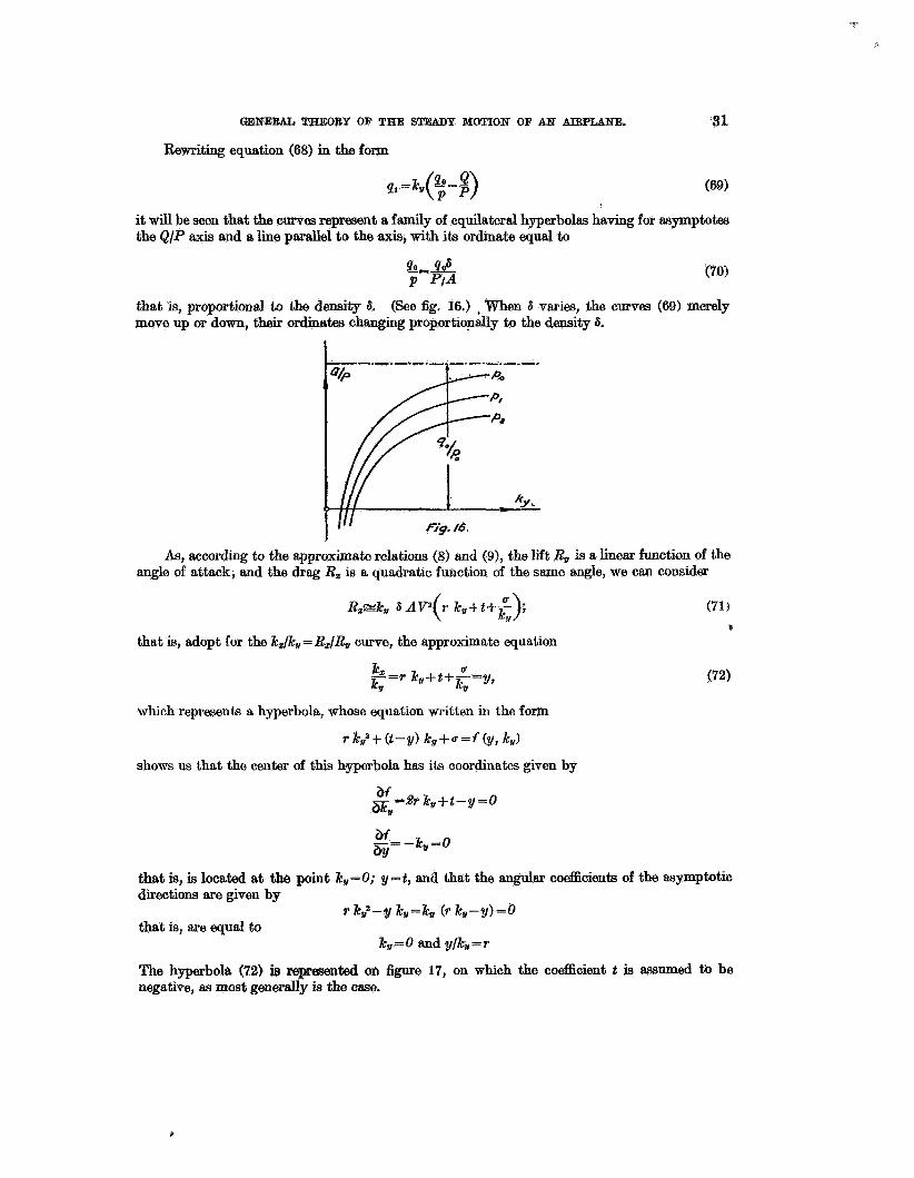
Bewriting equation (68) in the form

I

it will be seen that the curves represent a family of equilateral hyperbolas having for asymptotes the QlP axis and a line pardel to the axis, with ita ordinate equal to

that is, proportional to the density 6. move up or down, their ordinatea changing prop@iionaUy to the density 6.

(See Sg, 16.) , When 6 varies, the curves (69) merely

fig. /6

As, according to the approximate relations (8) and (9) , the lift R,, is a heax function of the angle of attack, and the drag R, is a quadratic function of the same angle, we can consider

~ ~ = k , 6 AVZ r k,-t-tfq)i ( k, that is, adopt for the k,/k,,=R,/R, curve, the approximate equation

(71 1 Q

which represents a hyperbola, whose equation written in the f o m

r k,? + 0 - y> k, + u = f (y , k,) shows us that the center of this hyperbola has its coordinates given by

that is, is located at the point k,,=O; 'y-t, and that the angular cdcienta of the asymptotic directiom me given by

rk,,*-yk,,=k,, (rk,,-y)=O that is, are equal to

k, = 0 and y/ku = r

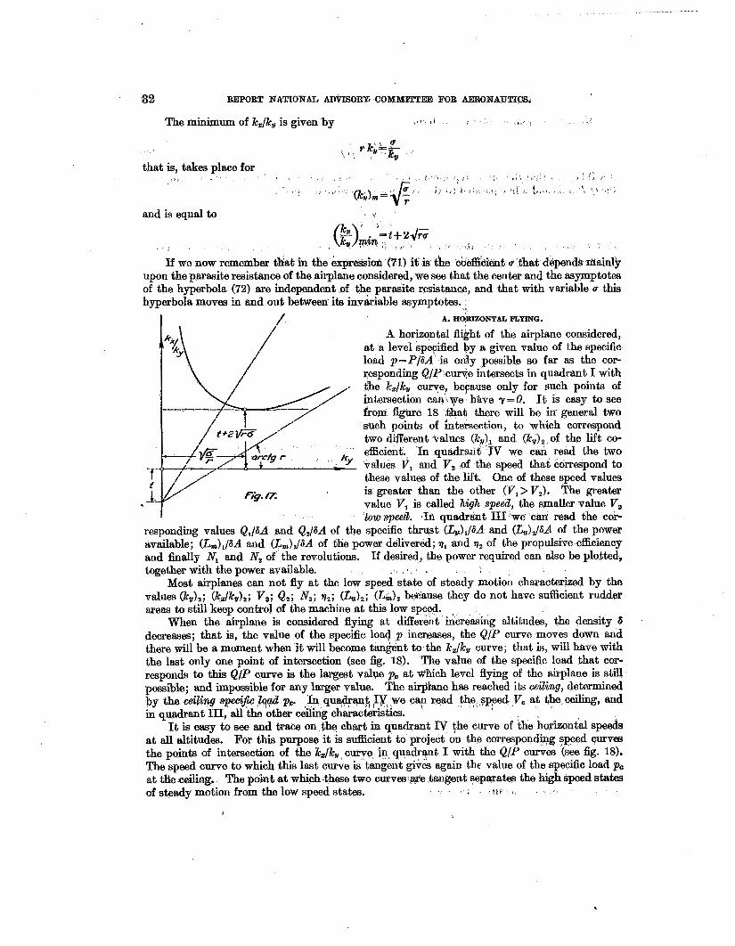
The hyperbola (72) is representad on figure 17, on whch the coefficient t is assumed tb be negative, tw most generally is the case.

32 REPORT NATIONAL ADVISORP, C0MM;l"TEB FOR AEBONAUTICB

The minimum of k,/k,, is given by t l

i

and is equal to

If we now remember that in the expressio& '(71) it is the co&&nt u that depenh mainly upon the parasite resistance of the airplane considered, we see that the center and the asymptotes of the hyperbola (72) are independent of the parasite resistance, and that with variable c this hyperbola moves in and out between its invariable asymptotes.

/ A. HORIZONTAL FLYING.

A horizontal fight of the airplane considered, a t a level spepified by a given value of the specific load p=P/GA is ody possible so far as the cor- responding Q/P c ~ e intersects in quadrant I with

awe only for such points of Wave r=O. It is easy to see there will be irr general two

such points of intersection, to which correspond two different values ( and (kw),,of the lift co-

' eBcient.f In qua& we can read the two -ky values V, and V, of the speed that correspond to

these values of the lift. One of these speed values is greater than the other (Vi > V,). The greater value V , is called high speed, the smaller value V, lowsped. pIh quadrant IIl 'we can mad the cor-

responding values &,/SA and of the specific thrust (La),/6A and (L&/SA of the power available; (Lm)#A and (Lm),/GA of the power delivered; q, and q, of the propulsive efEciency and jhally Nl and N2 of the revolutions. If desired, the power required can also be plotted,

Most airplanes can not fly at the low speed state of steady motion characterized by the values (7c,),; (k,/k,),; V,; &,; N2; qa; (L&; (&J2 bebause they do not have sufficient rudder areas to still keep control of the machine at this 1

&creasing altitudes, the density 6 decreases; that is, the value of the specific load p increases, the Q/P curve moves down and there will be a moment when it will become tar$ent to the k,/k, curve; that is, will have with the last only one point of intersection (see fig. 18). The value of the specific load that cor- responds to this Q/P curve is the largest valve p, at which level flying of the airplane is still possible; and impossible for any larger value. The ah$lane has reached its ceiling, determined by the ceil<ng speDeciific lqzd p,. Iq qur$rant iq we can read the s p l d V, at the wiling, and in quadrant 111, all the other d i characteridtics.

It is easy to see and trace on the chart in quadrant N the curve of the horizontal speeds at all altitudes. For this purpose it is sufficient to project on the correspon- speed qurves the points of intersection of the k&, curve in. quadrant, I with the Q/P curves (see fig. 18). The speed curve to which this last curve is tangent gives again the value of the specific load pc at the ceiling. The point at which .these two curves ma tmgeut separates the high speed states

together with the power available. . . ,

When the airplane is considered flying at

of steady motion from the low speed states. ' ' " I t C ' L '

?

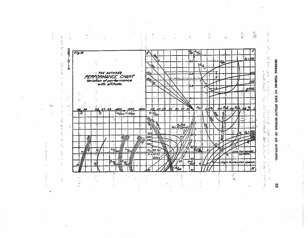
1 .*

I

34 REPORT NATIONAL ADVISORY CO-E FOR AERONAEPICS.

Making use of our approximate equations (68) and (72), we may find the values of the horizontal speeds at all altitudes from the condition QIP=kx/kyt that is

I (73)

(74)

L

or

1

Replacing k, by its value I

$ 6 (75)

From which equation we find

and {or the horizontal low speeds, the values: I

The ceiling is given to us by the condition

that is, i v, F= v, (78)

(79)

( ~ o - t ~ ) ' =4(a $. a i ) T p (80)

I shall remark here that the quantity t p is in general small (on account of t being small) in comparison with qo, so that, as a Grst approximation, we can replace the condition (80) by the approximate condition

d = 4 b + ql)rp2 (81) from which we find:

(a, - @P - TP2 4(a+pJ2 (a+nl)

or

and finally for the ceiling density we get the value

(83)

With the same approximation ( t g 0 ) the ceiling speed V, bas for its value

and the corresponding value of the lift coefficient is equal to

(85)

It is easy to see that this last ceiling lift value is somewhat larger than the value of the lift .-

<7c,,m =

at which k&, is a minimum.

GEMEWL THBOBY OF THe STBADY, MO!CION OF AN AIRPLAN% 35

It is worth natice that the power required for horizontal flying

R,V= k 2 A P = P p ~ & + @ ~ ~ a ( r k ~ t ? J + ukv-9

has a minimum for a lift value (7& given by

and equal to

Usually ql is of the same order of magnitude as 4, thus (kw),, being greater than (k&, has a value close to (k&

As has been mentioned already, the ceiling of an airplane is characterizad by the value p, of the specific load, but the ceiling density6, depends upon the weight P, that is, upon the loading of the airplane. The loading of each airplane can be increased up to such a value that its ceiling will be dropped to the ground level. The value of this limiting bad Po is given by

where 6, is the ground level air density. Hence.

(88)

It is of interest to add to the specific thrust curves of quadrant 111, also the two families of the following curves.

In the first place, the curves of Rx/6A as a function of V with p as parameter. Since R,/R,=kx/kc,, we obtain these curves directly on the chart by transferring the ks/kw curve of quadrant I to quadrant 111 by the aid of the speed curves of quadrant IV, and transfer lines of quadrant 11. Each speed curve and straight line corresponding to a given value of p will allow us to get one RJSA curve in quadrant IV for the same value of p (see fig. 18). Since

R & $ j A V 2 ( rkw+t+ F) and k,Va=p,

these R&A curves have for their approximate equation

or

With p as parameter, this equation represents a family of hyperbolas whose envelope is given by the relations

3 =$ + pt + 4 vs.

~

and has for its equation

I n the second place, the curves of Rs/6A as a function of V but with kw as parameter. In order to plot these curves in quadrant 111, it is suEicient to transfer the kJkU curve of quadrant I

, _.", " ,., . , _ _ ,,, ,,,, ...~. "" 'l,,

36 REPORT' NATTONAIJ &DTHORY COMM'JTIXE FOR AERONAUTICS.

to quadrant 111, keeping for*emh trace& c m e ! E,, constant, and makk@tW curves of quadrant IV, and transfer lines of quadrant I1 for each value of k,,. way that these curves haveh8een traoed on figure 18. ' Tliese eumm'have for their approximate equation

k$+t k,,+u> (92)

the horizontal axis as'thb axis of symmetry and p as The parabola that corresponds to the minimum of (r kV2+t k,,+u), that%, to he

~

I " , I

I sa i l ' i and represent a family of parabolas

parameter. ,phimum of R, for a given V, which takes plqce for

I , r t %

has for its equation

and is the outermost of all the other parabolas of the f d y . pis limiting parabola is the envelope of the fdmily of hyperbolas defined by equation (90). (See fig. 18.)

The point in which a &/SA curve cuts a Rx/SA curve with p as parameter gives us the hori- zontal speed for the corresponding value of p , and the RJ6A curve with k,, as parameter passing through that point gives the corresponding value of kv

B. CLIMBING.

If, starting from a given state of horizontal flying, the pilot by moving his stick varies k,, (see fig. 18) we can immediately see on the chart what value the path inclination will take. We shall be able easily to follow on the chart how y, V, Q, L,, L,,'?f, and Nwill vary with variable k,, but constant p. A decrease of k,, will bring us to negative values of y, the airplane will go down. The path inclinatioh y will pass through a maximum and decrease again until we reach the slow.speed horizontal flight. Since for each value of k,, we know the corresponding values of y and V, it is easy to compute the rate of climb

We can trace in quadrant IV the,rate of climb curve as a function of lc,,, plotting U on the V axis (but on a different scale). In such a way the U curves on the chart of figure 18 have been obtained for different values of p.

The maximum rate of climb decreases with increasing specific load until i t becomes equal to zero at the ceiling.

Let us calculate the value of U using our approximate equations. We have (with tS0)

An increase of kq, will casise the akplane to climb.

l?=yV

and with k,, Vz = p the rate of climb is found equal to

GENEBBL THEORY OF THE STEADY MO%IW OF AW AXRPLANE. 37

The rate of climb will be a maximum for

that is

which gives

or, on account of (82),

This value of k,,, when introduced in (95), will give the maximum value of the rat U corresponding to each value of the specific load p.

The value of H, at which the "best climb'' takes place in general increases with the altitude and reaches its largest value at the ceiling. But the ceiling value of kv is generally not greatly dierent from all the set of values given by (96); and since, on the other hand, a function does not change much near its maximum the rate of climb computed will not be greatly different from its maximum if it is assumed to take place at a constant lift equal to the ceiling value,

(kJ0 = @ with which the ceiling will always be reached.

The rate of climb, with ku having this value, is equal to

where

since, on account of (82) and (8b), we have

Po = 2rpo(ku)o, t (99)

we can put the expression (97) of the rate of climb in the form , r , % r

,The rate of climb at ground level is equal to

' uo= &(%mi- G o > (101)

Let us calculate, under the condition of a climb with IC,= (7c,), the tizhe of climb t , from ground level, characterized by the value po of the specific load, up to thelevel of specifio, load P < Po*

'According to the relations (45) and (47), we have for an isothermic atmosphere

. ,, dp=daRT= 7 u d H * ,

where here p is the atmospheric pressure. Thus

au d H = --RT U

38 REPORT NATIONAL ADWSOBY GOMMIrPEE FOB AEBONAVEIOS.

But, since

where here p is again the specific load, wy find

a=-= dH RTd2, PU

Making use of the value (97) for U and integrating, we get

t = R T r apW - pals

Substituting p'12 = 2 we get

or t = 2 R T r -f?.-. z0 a- bz2

On account of (98) and (82) we have

J2 = bzc= b Jg= J%, and thus

Taking account of (102) we finally have:

The last two formulae give us the time of climb in an isothermic atmosphere of temperature T, from ground level up to the level of speciiic load p. For p = p c the time of climb turns out to be infinite. There is nothing atonishmg in this last fact because the reaching of the ceiling is an asymptotic phenomenon.

Formula (104) applied to the isothermic atmosphere of zero degrees centigrade T= 273O and the time t expressed in minutes, gives

Let us ha l ly find the direct relation between the rate of climb U-with IC,= (k,),-and

According to (102) we have the altitude H in the isothermic atmosphere.

j ~H=R#$ (106)

Integrating this last relation, from ground level up to the altitude of specific load p, we get

P H = RT 1s- Po

GENERAL THEORP OF THE STWDY MOTIOH OF AN -LANE. 39

The ceiling altitude is eqnal to

H,=RTQ& (108) Po

Subtracting (107) from (108) we fhd:< (H,-H)=RTQ PJP=Z (109)

where z is the altitude below the deiling. F'rom thia relation we get

Substituting these last values in (100) we find

Developing Sinh in series, and keeping only the h t term, which is a suflicient approximation even for the highest altitude actually reached, we find:

For the ground level

We thus also have

a= Uo(l-g-)

The two formulae (114) and (112) show us that as a first approximation, the rate of climb is a linear function, of the dtitude H .

As a result of long experience in the measurement of rates of climb of airplanes, in free flight, it has always been observed that the rates of climb appeared to be linear functions of the latitude. This fact brings us to the conclusion that all the assumptionS we have made in the foregoing really constitute an approximation practically fully sufEcient and that, to the approxi- mation with,which we actually measure rates of climb, the climbing takes place as if the atmosphere was isothermic. One can thus see that the isothermic atmosphere appears to be quite as good as any other standard atmosphere, but in addition the isothermic atmosphere has all the advantages of being the simplest conventional atmosphere.

It is easy to deduce from formula (114) the time of climb as a function of the altitude. We have,

and integrating we get:

The formula:

Hc He t=-lg - 27, e He- H

gives the time of climb in minutes, from ground level up to the altitude H < He. If we take conventiodly H=O, 95 H , we find

(1 18) HC

0 0 &In=O, 05-

40 BHPORT NATIONAL ~&DVISORY'BWWXWI!WiFOa~'AEROXfAUTIGSP 8

We will get the exact expression for the time of climb in an~isotbmichtuhckphab, if wCi use in equation (115) the value (111) of the rate of climb. We thus obtain

at=

and,integrating we k d :

or, since < < 4 a "

we'hally find:

(119) C ? *I T S I

, . , I I . 9 $ 3

This last formula gives the ex othermic atmosphere of absolute temperatureT, from ground level up to the altitude H < H c where 0, is the rate of climb at the ground, and the whole cli ib is supposed made at a constgnt ;value .Sf the lift coeflicient k, q u a l to its ceiling value (k,JC.

' 8

C. ENGINE THROTTLING A N D GLIDING. . / .

Until now we have considered the flight of the airplane at full throttle opening and variable altitude. Let us now consider the flight 05 the &plane at constant altitude, for example close to the ground level, but with variable throttle. Returning to our chart, we see that the ksI7c, curve of quadrant I is not affected by%he thkottle; the speed h ~ e s of quadr'awt3V and trdnsfer lines of quadrant I1 ar cted by the throttle; but the spec%c*tkbt curires of quadrant; I1 'depend directly u ttle opening. Proceeding as was indicated 31 the chapter dealing with the engine-propbller system, it will be erisy to compute the cupves of specgo t h t as a fuflctiofi of the speed foPdif€erent throttle openings: &o (full throttle), k I J z:; x3 set of such specific thrust hrves 'have bees represented in figure 19. A' tscfiatian of khe 6hrottle

e erigirid power, whibh brings t@ith it a shifting of the bpecifia tkhst CU-~B. the throttle is'reducbd. ''IIU tWextensioet of

I quadkant I11 have be different throttle openings &,, &, lxZ,

now a complete reprksentation o€ %he openings.

, Once the set of specific thrust with vtkiable throttle is established, it is easy to plot in quadrant I the corresponding @P d&bs, making use of the speed curve and transfer line of the altitude considered, the throttle opening being now our #mtmet;er!"Th0'ohmt thw,completed, the influence of the evihe,;thrott% on the flight of the airplane becomes self-evident.

Let us consider the airplane first flying at full throttle opening xo, at a certaiih value of k?,, the inclination of the flying, pith to t? horizontal, having the value y. (See fig. 19.) The corresponding value of the s'peed is given by the speed curve of quadrant IV, and the other flying characte+stiq. cw, ;be irA to throttle the engine, the path the throttle opening z3, for example, the, not be afected-provided the action of the&+stream on the rudders can be neglected, as hiis

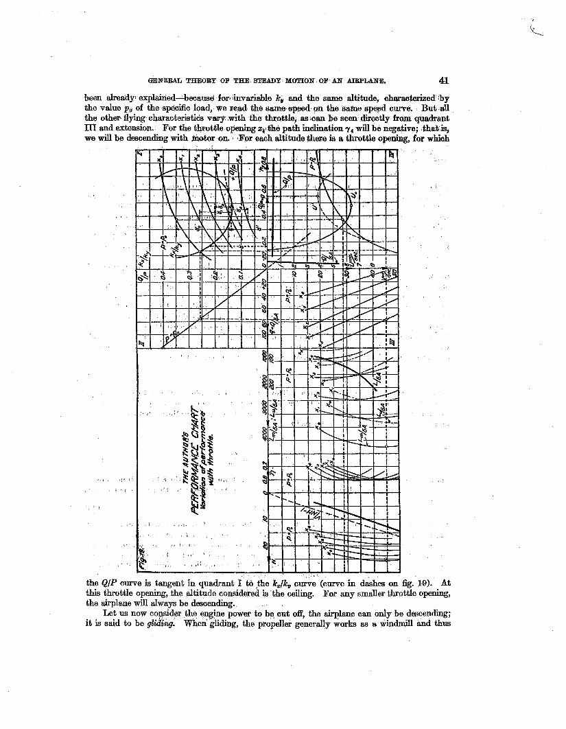
43.

been already: explained-because: $or] invariable kv and the same altitude, charackked' by the value po. of the specific load, we Bead. the same.epeed on the same speed curve. But all the other flying characteristids v q with the throttle, tsican be seen directly from quadrant m and extension. For the pening xA1 &e path inclination yr will be negative; *that is, we will be descendkg with 2 $For each altitude there is a throttle opening, for whiGh

GEHERAL THEORY OF THE STEADY 8 M W O N OF, ILN AIRFIANE.

the airplane will always be descending.

it is said to be glidwg. Let us now coyides off, the airplane can only be descending;

generally works as a windd l and thus

42 REPORT NATIONAL ADVISORY COMMITTEE FOR AERONAUTICS.

wi l l give us a negative thrust. We cam plot for the altitude considered the -Q/P curve on the negative extension of the axis of quadrant I (see fig. 19); we shall then be able to read, for each value of k,,, the exact inclination 7' of the airplane gliding trajectory, between the k&,, curve and this -Q/Pbcurve.' The gliding speed wi l l be read in quadrant N on the same speed curve. FOF large values of y', corresponding to small values of k,,, we shall get a more accurate value of the speed in gliding by taking for its value V -@-, as has been already explained. The rate of descent is equal to

U' = Vy'

and can be computed easily for each value af k,,, as V and y' are knowa Tbe curve of the rate of descent has been plotted in dashes in quadrapt I V of figure 19, using for it the same scale as for &e rate of climb. It is easy to see that the minimum of the rate of descent U' does not coincide with the minimum of y', the last being a minimum for k.Jk,, minimum; the value of IC, that makes U' a minimum being larger than the one that makes 7' &.imum. We now see that, if an airplane is gliding at a certain value of k,,, and if we slightly open the throttle, it is not the speed that is changed, but only the gliding path; the angler is decreased, and the rate of descent is reduced in proportion.

We can transfer the - Q/P curve of Quadrant I as well as the -&/Sa curve of Quadrant 111, by the aid of the speed curve and transfer line, using for that purpose the negative extension of the specific thrust axis. The -&/Sa curve thus obtained is represented by a thick line on figure 19. By the aid of this last curve we can deduce the mechanical losses of the engine when the law of variation of the engine revolutions with the speed in gliding is known. Such a curve of the revolutions in gliding as a function of V i s represented by a thick line at the end of the extended Quadrant 111. The fact is, that when gliding, the propeller generally rotates at a much less number of revolutions than its regular number of revolutions and thus works as a windmill, with a relatively high value of the advance V / N . But under such conditions, the efIiciency of q' of the propeller, working as a windmill, will be very closely equal to

IYH "=v where H is the efective propeller pitch.2 Thus, if for a given value of the gliding speed V we know the corresponding -&/SA and N , we have the power absorbed by the propeller working as a windmii equal to Q V, and the power delivered by the propeller to the engine and absorbed by the last as mechanical losses L equal to

or L = q ' Q V

- L Q Q ,..=q'V -= N H - 6 8 6A

The curve of L/6A is represented in the extension of Quadrant 111 by a thick line. we assume the mechanical losses we get

The negative thrust given by the propeller when gliding would then appear to be constant at all speeds.

If we wish, when gliding, the propeller thrust to be exactly equal to zero, yp must adjust our throttle in such %way that the ratio V l N H is nearly equal to unity, because, as is known,S for V/iVH=l the propelller thrust is equal to zero. The propeller revolutions will then vary proportionally with the speed according to the relation

' N = V / B t (124)

If in addition to be proportional to the revolutions, that is, we put L = f N ,

Q = f l H (123)

Practically, the negative t h m t in a glide does not appear to vary greatly.

1 I owe tbis last remark to m y assistant, bfr. W. F. Gerhardt, aeronauticalenglnear at XcCimJk Field. I See ''General Theory of Blade Screws," by Dr. G. de Botheest, Chapter IL 8 For= exact disoussion of this question 888: "Qeneral Theory of Blade above mentioned, Chapter XI.

GENERBL THEORY OIP T€@ S ~ ~ ~ q d O T I O H OF AN A I W E . e43

where H is the propeller pitch. The curve of N as a function of Vwill be a straight lime-repre- sented in dashes at the end of Q,uadrant 111 extension of @e 19. When gliding under such conditions, our &/P curve will b to the E,, axis, as its ordinates will all be equal to zero. The inclination of our gliding p e mehured simply by the ordinates of the curve (see fig. 19). We thus see that when gliding, the propeller acts as if the increased, and power has to be applied in order to eliminate this effect.

One can now see how complete a picture of the properties of an airplane m s is given by the chart developed in this paper, and with what ease this chart allows us to the variations and mutual inter-relatiow of dl the quantities involved in the problem.

The approximate equations we have deduced for all the curpas of the chart may be ysed in many cases for a h t checking, but attention must be paid to all the assumptions made in deducing these approximations. The approximate equations applied under carefully considered limitations give very good results for some problems, but for any general and broad discussion connected with the study of an airplane in stebdy motion the general method of the chart must be used.

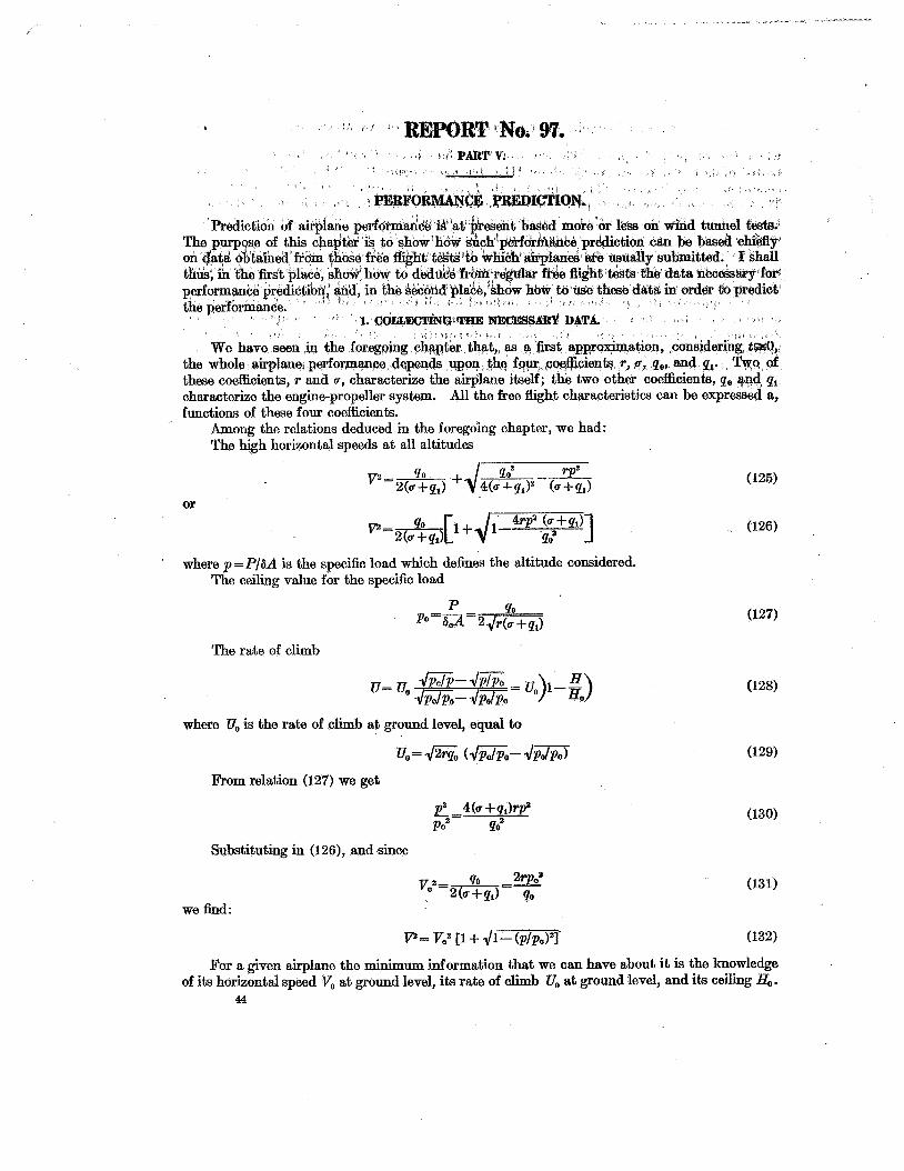
ord*or lbss on wihd tuninel €eats.

j

the whole aisphe, ped these coefficients, r and

functions of these four coefficients. Among the relations deduced in the foregoing chapter, we had: The high horizontal speeds at all altitudes

or

where p = P/6A is the specific load which defines the altitude considered. The ceiling value for the specific load

The rate of climb

where 0, is the rate of climb at ground level, equal to

From relation (127) we get

Substituting in (126), and since

we find:

For a given airplane the minimum information that we can have about it is the knowledge of its horizontal speed Vo at ground level, its rate of climb 0, at ground level, and its ceiling Ha.

44

GENJ3BAL TIBOBY OF THB STEADXI&EO%EON OF AN AIBPLAXEL 45

Let us try to find the espresr;tions for the &dnr,co&c@nts P, ur pol mdr,qQm functions of the& last quantities V,, U,, and H,. We shall then be able to cornputs. the dour charact&istic CoefEcients r, u, p,, and p1 from the o,rdbwy $reg%light. t&ts.

When the ceiling Ho t i

which giuea

Knowing V,, we h d

Enowing pa and 0, from (129) and (131), we d d I t

and solving these two equat . I

137) 1 . I ) I and

' 1 ' 2

and knowing po from (131), we get

+ (139)

It is clear that if only three conditions &e given us which we have assumed to be the values of V,, U,, and 3, we can k d only three relations contbining r, u, p,, and p, as functions of Po, U,, and Ho, and we have just found the expressions for r, pol and (u+pl) in terms of V,, Uo,* and po. A fourth condition has thus to be put forward in order to specify fully the problem. But it must be remarked that so far as wk intend to predict only the horizontal self-speeds at all altitudea, the rates of climb at all altitudes, t g apd th9:fime of .climb, we 40 not need to know separately the c d c i e n t ~ o,wd p1 .became, as oan be seen from the relations (125), (1281, (1331, and (1171, the quantities V, ZT, H,, andrtmit, are functions onlys .of r, pol and ( ~ f p ~ ) ~ But as Eioon as the propell? efficiency qp k r horjzon$d flying at grouqd level known, we shall immediately be able to find p1 and thus know the separate values of 4 and pl. In effect we have * f

(140)

where Lo is the power delivered by .the ,engine foi .hb&zoiital flight a t groimd level, which in any case must be considered a l inoh qsaatikf.; :F@o~h the%kt relation

< * ? z * I 3 , ~ . . i

or, since q,,Lo=QoVo, where Q0 is the propeUer t k t for haizontd.flying at ground level, and using the notation

we finally get

5 @ J O L Q O f I

PI-- v,

I .

- @ d o p

(141) L%J"?PQ

46 REPORT NATION& &DVISOBY C0XMI”EE FOR bE&ONAU!EICIS.

The value of the coefficient q1 once found, we can find the value of u by the aid of relation (139). Thus, when we know:

Vo, uo, Ha, tloi and Lo we can deduce immediately the values of the charac&istic c d c i e n correspond to the airplane considered.

Unfortunately the propeller &ciency is the quantity that most generally is the least known among the quantities affecting airplane performanee. That is why it may be of interest to attempt to check this efficiency, when unknown, e y n only to a first approximation.

We have seen in the foregoing that the value of the lift coefficient a t which the ceiling is reached

is generally included between

that is, included between the lift value at which kz/k,, is minimum and the lift value at which E z / k ~ ‘ ~ is a minimum (“power required minimum”). It is clear on the other hand that the value of p1 depends upon the propeller of the engine-propeller system considered. There is advantage in selecting such a propeller as would give us qI = 2u, because we would then have (kJ0 = (3cy)p, the power required would be a minimum at the ceiling and the highest ceiling would be reached with the power available. But it is difEdt to expect that each airplane is fitted with the best climbing propeller and that is why in general p1 <2u. Let us designate by n the ratio

a

pr,, U (142)

It is easy to see that for high ceiliig airplanes the ratio n will be close to the value 2, and for average ceiling machines closer to 1. By making in (139) the coefficient p1 =nu we get

It is by estimating the value of n that one can decide to a first approximation upon the relative values of u and pl. It must be remarked that it is only the value of the propeller efficiencies that will be affected by the value adopted for n, because all other performance char- acteristics, as has already been mentioned, depend only upon (u+ql) and thus are independent of the value of n.

Let us designate by N’, q‘, and L’, the number of revolutions, the propeller efficiency and power delivered at ground level for E,,= &),-at that moment the airplane is climbing with the rate of climb Uo and has the self-speed V ; let us designate by Nu, q,’ and Lu, the number of revolutions, the propeller efficiency and power delivered at the ceiling; and by No the number of revolutions for horizontal flying a t ground level; and let us try to find the expressions for q,,, q‘, and qu in terms of the characteristics of the airplane performance. We h a y :

and

we iind

L '

(147a)

On account of ~ 2 I

and replacing r &d u by their values (137) and (143ywe find: * I

(145b)

(146b)

(147b)

where

n l-- p' = 2(1+n)z2

1-22 ,

n+2

%(1-22) pg = 2 m

and t I I 1

I % - d P X C 1 , I I

The curves of po, p', and pD as functions os 22 for h= 1 and a=2 have been represented on @e 20. It is easy to see from this figure that in the foregoing formulm the value of n has a sensible influence on the value of pol a somewh influence on P O , but that P' turns out t? depend only very slightly upon n, especially values*of 22, that is for airplanes of high ce-. Thus by the aid of formula (145b) it is diff;cult to check the efficiency qo; by the aid of fornula (147b) the efficiency qu can be checked only to a rough approximation; but the effi- ciency q' can be fairly well predicted by the aid of the formula (146b). ' -

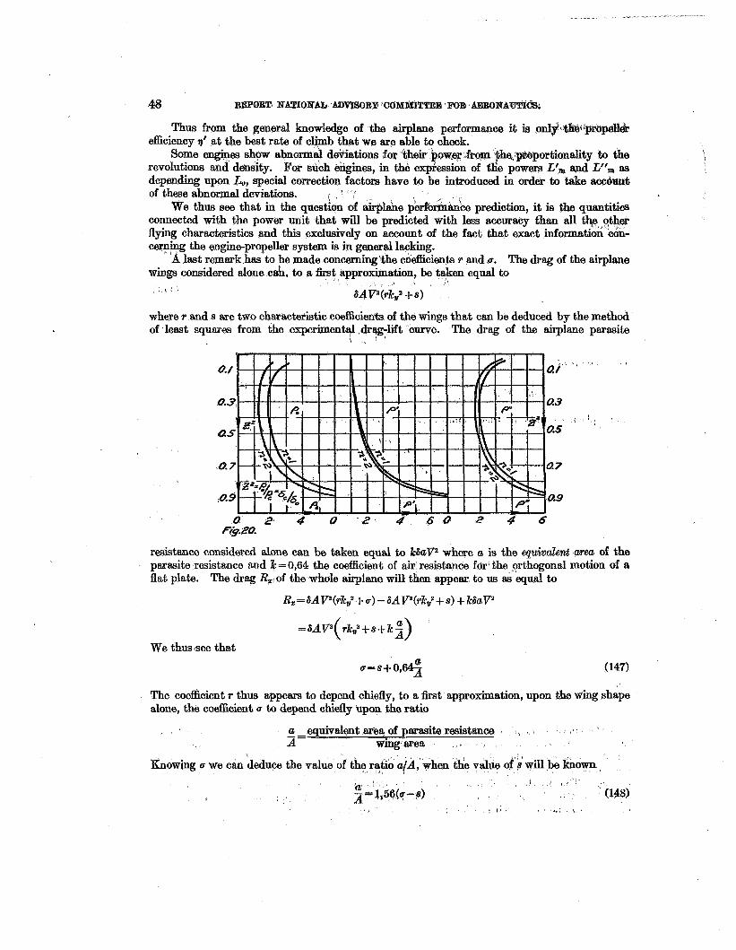
Thus from the general knowledge of the airplane performance it is o ~ ~ ~ ~ i ~ r ~ ~ e ~ efficiency B' at the best rate of clipb that we are able to check.

Some engiaes show tom fhe:p&portionality to the i revolutions and d-ity. of the POW= L'm a d L"m as depending upon Lo, sp of these abnormal deviations.

connected with the power unit that will be predicted with less accuracy flying characteristics and this exclusively on account of the fact that e m

last remark has to be made concerning'tihe coefficients r and (r.

to be introduced in order to t&e accburrt

ce prediction, it is the quantitiea W e thus see that in the question of airplahe

' the engine-propeller systern is in general lacking. The drag of the airplane

wings considered alone cab. to a first appr ation, be taken equal to L 1

SAVz(rk,,2 3.8)

where r and s are two characteristic coefscienk of the wings that can be deduced by the method of least squares from the experiment4 &rq%-lift curve. The drag of the airplane parasite

I t )

s i

L

Ft9.20.

resistance considered alone can be taken equal to k8aV2 where a is the equivalent area of the parasite resistance and k = 0,64 the coefficient of air resistance fdr bhe 'orthogonal motion of 8

flat plate.

R~=sAVz(rk, ,2+u)=S8Va(rk~2+~) +kSaVz

The drag R, of the whole airplane will then appear to us as equal to

We thus see that a

U= 8+ 0,6%

The coefscient r thus appears to depend chiefly, to a first approximation, upon the wing shape alone, the coefficient u to depend chiefly kpon the ratio

a equivalent area of parasite resistance I . 2= wing &rea I (

Knowing u we can deduce the value of the value of 8 will be known

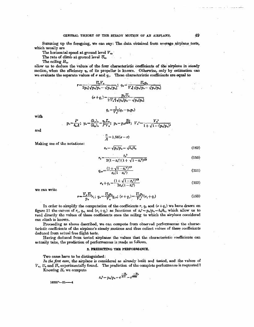
GENERAL T-ORY OF THE S-Y MOTION OF AN AIRPLAm. 49

Summing up the foregoing, we can say: The data obtained from average airpl

The horizontal speed at ground level Vo, ' The rate of climb at ground level Uo, The ceiling Ho,

which usually are

&ow us to deduce the vcilues of the four charaoteristic coeifTicienta of the airplane in steady motion, when the efljciency rl, of ita propeller is known. Otherwise, only by estimation can we evaluate the separate values of u and pl. These characteristic coe3bient.a are equal to

; po= uovo

T- 2p.t.JiJG- . J i i K I

1 nl=y,z(no-YoPo)

with

and -J= a 1,56(~-8)

Making use of the notations: zo= m o = m o

we can write

In order to simplify the computation of the coefficients r, po and (u+pl) we have drawn on figure 21 the curves of rl, pol and (ul+pl) as functions of ~2=po/po=6, , /60 , which, allow us to read directly the values of these coeBcients once the ceiling to which the airplane considered can climb is known.

Proceeding as above described, we can compute from observed performances the charac- teristic coefficients of the airplane's steady motions and thus collect values of these3 coefficients deduced from actual free flight tests.

Having deduced from tested airplan- the values that the characteristic coefficients can actually take, the prediction of performances is m d e as follows.

VO,

2. PREDICTING THE PERFORMANCE.

Two cases have to be distinguished: In t h j m t case, the airplane is considered as already built and tested, and the values of Uo and H. experimentally found. The prediction of the complete performance is requested a

10355°-214

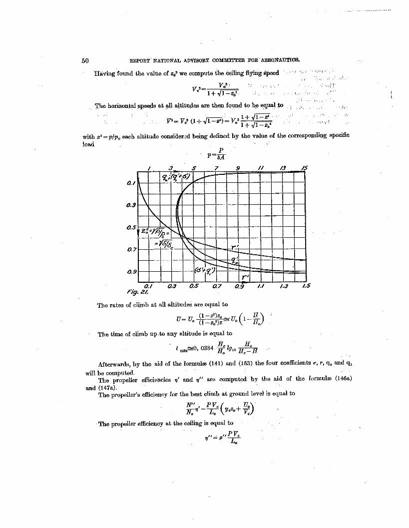
50 REPORT NATIONAL ADVISORY COMEKITTEE FOR AERONAUTICS.

B a i n g found the value of zo* we compute the ceiling fkybg s F d

The horizon,tal speeds at altitudes are then found to be 0

with za = p / p c each altitude consider,>d being defined by the value of the corresponding specific load

Y * P = a

The rates of climb at all altitudes are equal to

The time of climb up to any altitude is equal to

Afterwards, by the aid of the formula (141) and (153) the four coefficients rr, T , q, and q1 will be computed.

The propeller efficiencies q’ and q“ are computed by the aid of the formulre (146a) md (i47aj.

The propeller’s efficiency for the best climb at ground level is equal, to

“he propeller efficiency at the ceiling is equal to

I 1.

GENERAL THEORY OR THE STEADY I MOTION OF A?S AIRPLANE. 5.1

Finally,. the whole performance chart can be,,traced to a h t apprmipation. The speed curves of quadrant N and t r a d e r lines of quadrant $1 are onlp geometdcal~ intermediaries and can be traced at once. The coe3icients r- and u being known, the kJcv curve of quadrant I can be plotted. The coefficients go and q, being the specific thrust curves of quadrant III can be plotted, the whole strip of curves being d to a h t approximation by a single

I can be traced. Afterwards, in extension of quadra& curve oa@bb pfdtted. Finally, by three points (qo, V,,), (qt7 V), (q”7 VJ the efficiency; c m e can be traced and thus the L&A curve deduced. In such a way, from the knowledge of V,, U,,, He, &,, and TI,, all the possible conclusions concerning the steady motion of the airplane considered will have been drawn.

In the second case, only drawings of the airplane considered are supposed to be available. It can be either an airplane in the process of design, or an airplane about which flying data are not available. The prediction of the complete performance is requested.

The values of the coefficients r and u axe first estimated by comparison with other similar airplanes. T w o airplanes having the same wing-profile will have very closely the same values of r. The value of u will be taken equal to

m e . Further, by the aid of the transfer lines and @e curves of~qu&ant

,

a u = s + O , 64- A

where the equivalent area a of the parasite resistance has to be estimated and s taken from data concerning the wings used on the airplane considered.

Further, the power Lo and the airplane weight P must be known and one must decide upon the value of the efficiency q,,. As we have

(154)

This last relation will give us the value of (ku), and thus the value of the self-speed V,, that is compatible with the power available and drag offered by the airplane considered.

The easiest way to get a solution of equation (154) is to p l o t h t the kJk, curve as function of kv-as we can do from the knowledge of the coefficients T and u-and to plot afterwards the curve of k.Jk$12 as function of k7,, by dividing the ordinates of the kJku curve by the corresponding values of 6

The smallest abscissa of the kS/kg3B curve corresponding to the ordinate equal to

Ilo Lo P P O ”

will give us the value of (iQ0 to which corresponds the high horizontal speed V,, which we will be able to read directly if only previously in our so-called quadrant IV, the speed curve p,, = ku P has been traced (see fig. 22).

Having found V, by the aid of the kJk$fi curve, let us consider the relation N‘ Il’L’&jq s’L,=P Vyc+PU*

from which we h d N’ - $Lo - P vy, NO Uo = P

(155)

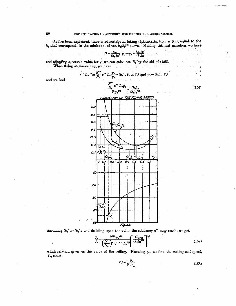
52 aEPORT N TIONAL ADVISORY COMMI!C!CEE FOR AFiRONAUTICS.

As has been explained, there is advantage in, taking (k,,)ccs(kir)r, that is (kJC equal, to the Making this last selection, we have kW that corresponds to the minimum of the kZ/l&,Ya c

(b)al v2=&; Yc=Ym=

WB. can calculate 0, by the aid of (155). ting a certain value for When 3ying at the csiling,*we have

Assuming (k,,),= (kv)x and deciding upon the value the eEciency may reach, we get

which relation gives us the value of the ceiling. V,, since

Enowing pc , we find the ceiling self-speed,

(158)

GENERAL THEORY OF THE STEADY MOTION OF AN AJXPLANE. 53

It is in such a way that an estimation of the values of V,, 0, and po can be reached. The characteristic coefficient qo can now be easily found by the aid of formula (153)) and the value of q, by the aid of the formula (141).

s

Finally, we have to verify, by the aid of the formula

how far the assumption (kJ0 = (k,,)M holds. The checking of the rate of climb 0, and ceiling pa by the aid of the last method givea good

results because we have to deal with values "of functions close to their minimum, where they do not vary much, the differences between y~ and yo, and between (kx)d(k,,)x3'2 and (kz)o/(k,,)081a being infact only very slight.

In all the preceding discussion, I had chiefly in view to point out the real nature of the prob- lem of the performance prediction and to show by what concatenation of ideas we can be brought ,

to its solution. Special attention must be paid to the r61e the kJk,,3/3 curve plays in the finding of the self-speed V, from the knowledge of the power available qo Lo, and the meaning of the minimum ( k x ) ~ / ( k w ) ~ 3 1 2 of the kZ/k,9l2 curve for the ceiling of the airplane considered.

The standpoint adopted in all this chapter was the prediction of the performance, stazting with the knowledge of the smallest amount of data available concerning the airplane considered. But when for a given airplane, we know its k.,/k,, curve and possess all the data necessary in order to plot the specsc thrust curve of the airplane's engine-propeller system; then the simplest way to predict the performance is just to draw, for the case considered, our performance chart, which will give the most complete performance prediction of the airplane considered. It is this question of bd -~ from free flight tests these two fundamental curves-the kz/k, curve and the specsc thrust curve-that we wi l l consider in the next chapter.

REPORT No. 97. PART Vi.

J!REE FLIGHT TESTING.

The performance chart we have developed in the foregoing gives a complete reppesentation of the performance of an airplane in steady motion. A complete free flight test of an airplane must thus consist in getting all the data necessary in order to establish such a chart. The speed curves of quadrant N and transfer l i e s of quadrant I1 being only geometrical intermediaries, it is only the curves of one of the quadrants I or III that we have to establish, because the curves of these quadrants mutually correspond to one another by the aid of quadrants 11 and IV. We shall show how to obtain from actual free flight tests the k&, curve and the QlP curves of quadrant I.

Let us consider an airplane equipped with the following instruments: An air speed meter, a barograph, a strut thermometer. The barograph will be consisdered to be calibrated in pres- sure units, which is the only reasonable calibration of these instruments when used for free flight testing. In order to control, to a certain measure, the power of the engine, a tachometer must also be available. The test can be made either at full throttle or a t any reduced throttle.

The airplane so equipped must make two or three climbs, at different indicated air speeds, but the last must be kept constant in each case all through the climb; also, on the way down, after each climb, it must make two or three glides. Each glide must also be made at different indicated air speeds, but constant for each glide. The glides will be done partly with the throttle completely closed and partly with the throttle so adjusted that

V --1 NH=

In therie last glides the propeller thrust will be practically equal to zero. The indicated air speed is proportional to the quantity

8 VZ 2 -

But since P ~ k f i A V z , we have

So that, if we keep 6Pl2 constant, that means that our glides or climbs take place at a constant value of the lift coefficient, and this is independent of our altitude.

Let us k t consider the data furnished by the glides, made under the condition V/NH= 1. The barograms obtained from those glides will give us the value of the pressure at each moment, and taking account of the corresponding temperatures, we can fmd the values of the densities 6 for each moment of the glide and thus can deduce the actual self speeds Vfrom the knowledge of the indicated air speeds and the calibration curve of the speed meter used. Further, the rates of descent can be deduced from the glide-barograms, which, as has been shown in Chapter 111, are equal to

lJ= -a-& dP

64

GENERAL THEORY OF THE STEADY MOTIOET OF AN BIRPLBNE. 55

where a=6g is the corresponding specific weight of the air and dp/& is the angular coefscient of the tangent to the glide barogram m r ~ e at the point considered. Know* V and 6, or the specific: load p-P/6A, we find from the relation kv=P Cos y / V Z , the corresponding v k,,. Sincelafor the glides under ,the condition V / N H = 1, we have Q=O and thus -y= - U/V, the point in quadrant I with the coordinates kq and - U/V will be a point of thq k&,, curve (seafigs. 18 and 19) ceeding in the same way for glides cated air speeds, we find a points of the k2& curve. The auth by the actual use of the above descfibed method that it is easy to get for values of i+,>(kJm by making glides at sufliciently low self-sp only to be made at heights suftient for the safety of the pilot.

When proceeding, as above described, with the glides made kith the throttle completely closed, we get a certain kz’Jk.’, curve. The dif€erence of the ordinates df this lagt curve and the kz/kv curve wiIl give us the -Q/P curve, which transferred in quadrant I11 by the aid of the speed curves and transfer line will give us the -&/&A curves, by the aid of which W? can estimate the mechanical losses of the motor, as has been already shown in the foregoing. (See

If now we proceed in a similar manner with the climb barogram, and recorded indicated air-speeds; that is, deducing from them the corresponding 6, V and y we obtain from each barogram a set of values of y corresponding to a constant value of k,,, for different values of the specific load p=P/6A for which we can adopt a set of standard values. If now we plot these values of y in quadrant I, starting from the kz/k,, curve and join all the points that correspond to equal values of the specific load, we get the family of the &/P curves, with aa parameter, since Q/P-k,/k,+ y in each climb. These Q/P curves, transferred in quadrant I11 by the aid of the speed curves and transfer lines Will give us the set of spec& thrust curves.

By tracing the rate of climb curves in quadrant I V the ceiling will be checked, and, as described in the foregoing, the whole airplane performance can be deduced with ease from the kaowledge of tho k,/7c, curve and the specific thrust curves.

If when making the last tests the airplane were equipped with a torque meter, then by recording the torque and the revolutions we would h o w the power delivered at each moment by the engine and we then could trace in extension of the quadrant 111, of our chart, the Lm/6A curve. As the La/6A=QV/6A curve can be directly deduced from the &/&A curve of quadrant 111, the knowledge of the Lm/6A curves will allow us to immediately deduce the efficiency curves. It is in such a way that from free Q h t tests the propulsive efficiencies can be deduced. It is easy to deduce from the eeciency curves and the Lm/6A curves, by the aid of the revo- lution curves as function of the self-speed V, the efficiency curve as well as the L & V 3 c w e as function of V/N, and thus to get from the free flight test the complete characteristics of the propeller. I t is also from the Lm/6A curve that the engine power characteristics as function of N for different values of the density 6 and throttle x can be deduced.

One can now realize how important it is to use a torque meter in free flight tests. A torque meter, giving us a continuous control of the power, will make the test perfectly reli- able in the sense of knowledge of the power really developed by the engine; and besides, the torque meter will allow us to obtain, in addition to the complete characteristics of the airplane, the complete and separate characteristics of the propeller and of the engine.

The chart (fig. 26) annexed at the end of this paper gives the characteristics of a Vought airplane as actually obtained from free fight tests by the above described method. For all the detaiIs concerning such test the reader is referred to the McCook Field (Dayton, Ohio) Report No. 1242, “ A repd showing the me of the de Bothezat perjbrmance chart for expressing the perf.rmance of the VE-7 airphne P-113, frm data obtain& in acltua2$ights,” by Mr. C. V. Johnson and W. F. Gerhardt.

I wish hally to call attention to one more important question connected with free-flight testing. The power of the engine is affected by the air temperature, and it is thus necessary to reduce the power of the engine, and thus the whole performance, to some standard tempera- ture, if we wish to get results that can be compared with other tests. For reasons that have

.

fig. 19.)

56 REPORT NATIONAL ADI~SORY COMMITT~E FOR AERONAUTICS.

been discussed in Chapter IV, it is the isothermic atmosphere of hero degrees dentigrade thW we adopt as standard, and thus the whole performance has to be reduced to zero ddgrees centigrade. It is evident that one has to take account of the temperature to find I316 vdae of the densities from the pressures given by the graph, but how knust we take idto account the influence on the performance of the power tion due to the temperature? ,

That is; at’thb same density But a t the temperature of zero degrees centigrade the engine wodd give a slightly different power from that in the actual flight. Let AL, be this positive or negative incr-ent of the power due to temperature differefi’w at constant density. On account of &e fact that’ the drag and lift of the airplane depend only upon density, neither ks nor &, nor V-bebtise P = k $ A P - d be affected by the temperatiwe; that is, neither the kJgTl cubre, nOT the speed curves. The increment of power ALm will act on the performance as a slight cbange of throttle and it is only the values of Q/P or Q/6A that will have to be corrected. As 6 and V remain the same, the efticiency q will remain the same, and the variation ALu of the power available will be proportional to the variation of the power delivered, but EB L,,= VQ and V remain the same, we have

Tne correction to be applied to the thrust thus simply turns out to be equal to

At a constant density, the engine power depends upon tdmperattire.

ALu = qAL, = VAQ

and the correction to be applied to the Q/P values turns out to be equal to

AQ rlhLm P - P V

The power correction AL, due to temperature at constant density has to be determined by special tests of the engine.

Those who have followed carefully the methods and questions of principles discussed in this paper will not meet the slightest trouble in making the most complete and rigorous airplane freeflight tests.

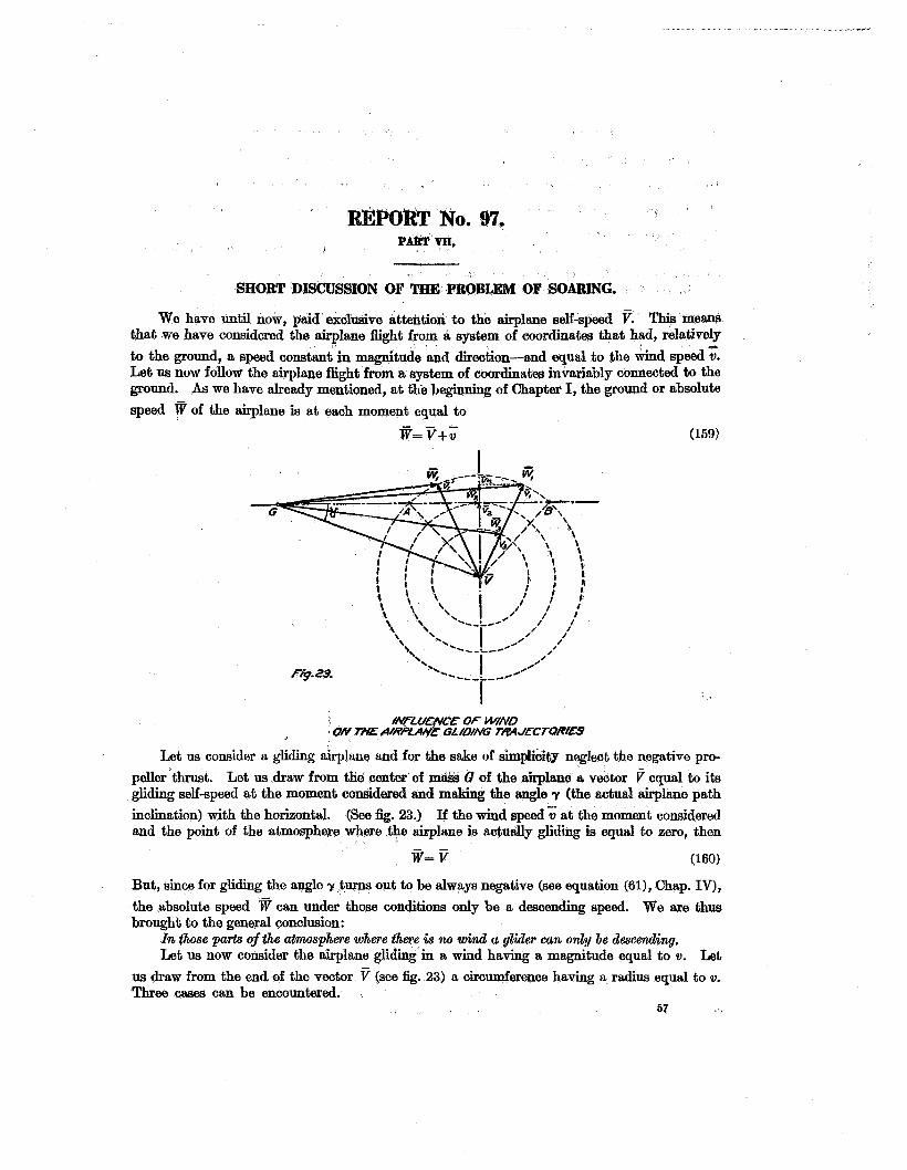
’ REPORT No. 91. i

PAkT

SHORT DSCUSSION OF THE PROBLEM OF SOABING.

We have until now, paid exclusive attehtioli to the airplane self-speed 7. This mean6 that we have considered the airplane flight from a system of coordinates that had, relatively to the gomd, a speed constant in magnitude and direction-and equal to the wind speed u. Let now follow the airplane fiight from a system of coordinates invariably connected to the ground. As we have already m&,ioned, at the%eginning of Chapter I, the ground or absolute speed W of the airplane is at each moment equal to

e= 7+u (159)

Let us consider a gliding airplane and for the sake of simpli&,y neglect the negative pro- peller thrust. Let us dram from the center of ff of the airplane 8 vector V equal to its gliding self-speed at the moment conaidered and making the angle r (the actual airplane path inclination) with the horizontal. (See fig. 23.) If the wind speed 5 at the moment comidered and the point of the atmosphere where the @lam is actudy gliding is equal to zero, then

jp= j7 (1600)

But, since for gliding the angle y turns out to be always negative (see equation (61), Chap. IV), the absolute speed %’ can under those conditions only be a descending speed. We are thus brought to the general conclusion:

In those parts ofthe atmosphere where there is no wind a glider can only be descendbq. Let us now consider the airplane gliding in a wind having a magnitude equal to v. Let

us draw from the end of the vector v (see fig. 23) a circumference having a radius equal to v. Three oases can be encountered.

57

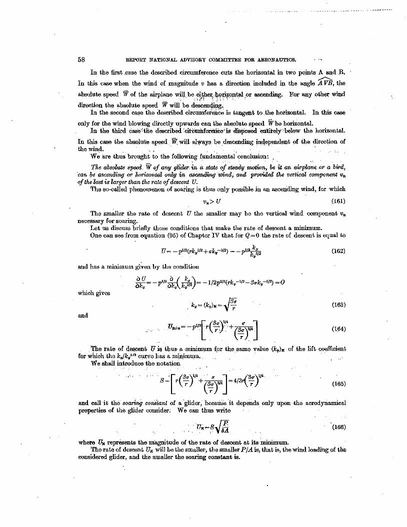
REPORT NATIONAL ADVISORY COMMITTEE FOR AERONAUTICS. - . 58

In the Grst case the described circumference cuts the horizontal in two points A and B. In this case when the wind of magnitude v has a direction included in the angle AVB, the

absolute speed @ of the airplane Foptal or ascending. For any other wind

direction the absolute speed i? In the second case the des tangent to the horizontal. In this caae

only for the wind blowing directly up absolute speed be horizontal. In the third case’the described ?is dk$osed m%3ely (below the horizontal.

In this owe the absolute speed W will always be descending independent of the direction of the wind.

A

We are thus brought to the follo

The absolute speed W of any glider in a state of steudy motion, be it an airplane or a bird, can be amend+ or horizontat only in ccscending &nd, and p r d e d the verEicaZ component v,, of the last is larger than the rate of descent U.

The so-called phenomenon of soaring is thus only possible in an ascending wind, for which

v,> u (161)

fundamental conclusion:

The smaller the rate of descent U the smaller may be the vertical wind component v,,

Let us discuss briefly those conditions that make the rate of descent a minimum. One can see from quation (95) of Chapter IV that for Q = 0 the rate of descent is equal to

(162)

necessary for soaring.

k u- - p1/2(&,1/2 + &,,-3/2) = - p’l- k,3/2

and has a minimum given by the condition

= - 1/2p1/2(& -112 - &k -612) = 0

which gives

and

?e rate of descent Z7 ia thus a .minimum for the same value (k,,)= of the lift codcient

We shall introduce the notation for which the i Q k , 3 I a cwve has a minimum.

and call it the soaring conshnt of a ‘glider, because it depends only upon the aerodynamical properties of the glider consider. We can thus write

‘(166)

where Ox represents the magnitude of the rate of descent a t its minimum.

considered glider, and the smaller the soaring constant is. The rate of descent Ux will be the smaller, the smaller PIA&, that is, the wind loading of the

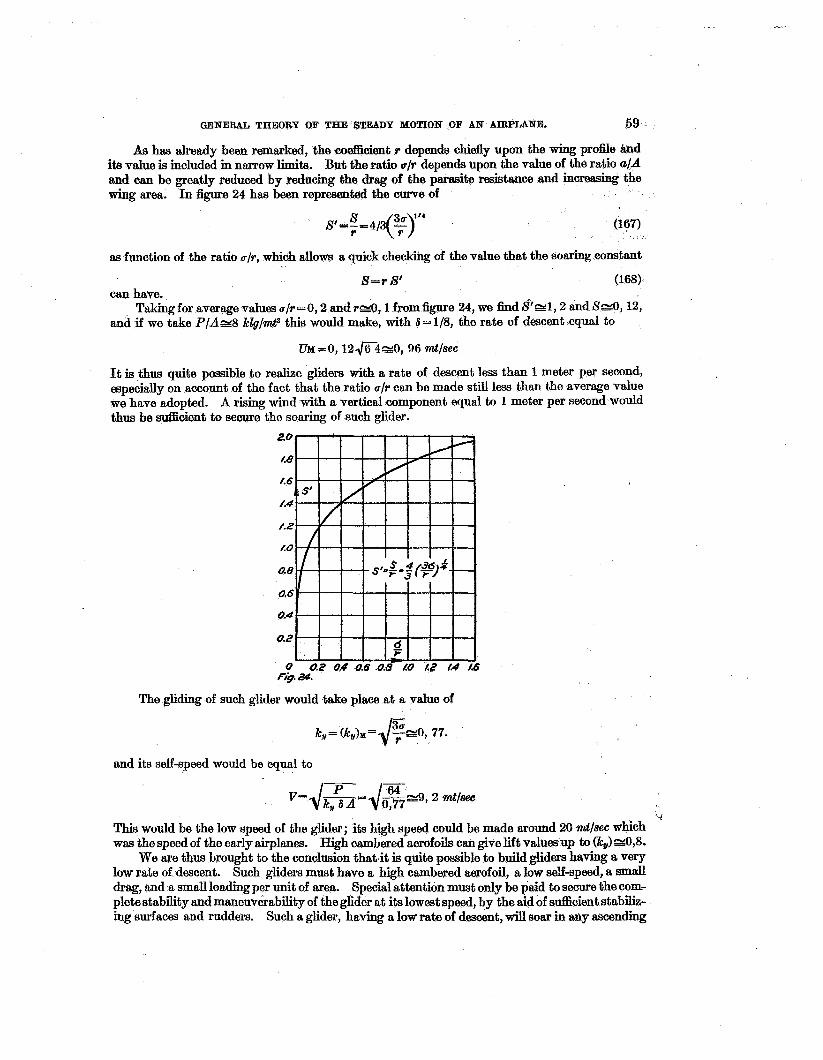
GENERAL THEORY OF THE’STEADY MOTION OF A H AIRPLANE. 59 ’

As has already been remaxked, the CoeffiGient r depends chiefly upon the wing profie And ita value is included in narrow limits. But the ratio u/9- depends upon the value of the ratio a/A and can be greatly reduced by reducing the hag of the parasite resistance and increasing the Wing area. In @e 24 h a been represented the curve of

(1

as function of the ratio u/r, which allows a quick checking of the value that the soaring constant

S = r 8’ (168) can have.

Taking for average values o/r = O , 2 and v z o , 1 from figure 24, we iind Pzl, 2 a$d SgO, 12, and if we take P / A r 8 klg/mtz this would make, with 6 = 118, the rate of descent equal to

UM=O, 1 2 F 4 r 0 , 96 mt/sec

It is thus quite possible to realize gliders with a rate of descent less than 1 meter per second, especially on account of the fact that the ratio a/v can be made still less than the average value we have adopted. A rising wind with a vertical component equal to 1 meter per second would thus be sufficient to secure the soaxing of such glider.

The gliding of such glider would 4ake place at a value of

k;= ( k J M = ~ ~ 0 , 77.

and its self-speed would be equal to

This would be the low speed of the glider; its high speed could be made around 20 mtlsec which was the speed of the early airplanes. High cambered aerofoiis can give lift values up to (kJ YO,8.

We axe thus brought to the conclusion that it is quite possible to build gliders having a v e v low rate of descent. Such gliders must have a high cambered aerofoil, a low self-speed, a small drag, and a small loading per unit of area. Special attention must only be paid to secure the com- pletestability and maneuverability of theglider at itslowest speed, by the aid of s&cient stabiiliz- ing surfaces and rudders. Such a glider, having a low rate of descent, w i l l soar in any aswnclmg

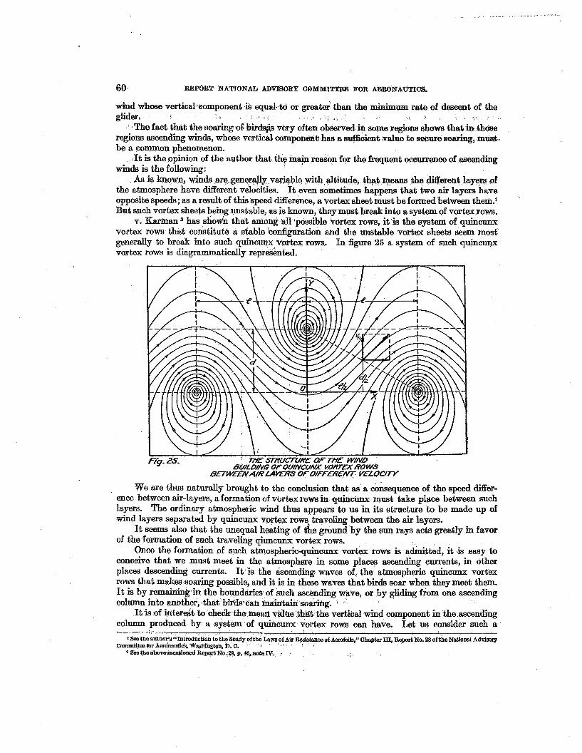
60 REPORT NATION& AJNISORY GOMM6ITTEE FOR MRONAUTICS.

wind whose verticalwxnponent4s equal. td or greater than the minimum rate of descent of the glider.

regions ascending winds, whose vertical compondnt: has a m.@uient value to swure soaring, musk. be a common phenomenon.

$It is the opinion of the author that thy mab reason for the frequent occurrence of ascending winds is the following:

As is ham, winds ax dy,vari+ble 6 t h altitude, thpt weans the different layers of the atmosphere have d It even sometimes happens that two air layers have opposite speeds; as a result of this speed difference, a vortex sheet must be formed between them: But such vortex sheets being unstable, as is known, they must break into a system of vortex rows.

v. Karman has showb that axtiong ail lpossible vortex rows, it is the system of quincunx vortex rows that constitute a stable 'configuration and the unstable vortex sheets seem most generally to break into such q u i n c v vortex rows. In figure 25 a system of such quincunx vortex rows is diagrammatically represented.

'The fact that the soaring 05 hi some regions shows that

cities.

We are thus naturally brought to the conclusion that as a consequence of the speed differ- ence between air-layers, a formation of vbrtex rows in quincunx must take place between such layers. The ordinary atmospheric wind thus appears to us in its structure to be made up of wind layers separated by quincunx vprtex rom traveling between the air layers.

It seems also that the unequal heating of &e ground by the sun rays acts greatly in favor of the formation of such traveling q iuncm vortex rows.

Once the formation of S U G ~ atmospheric-quiucunx vortex rows is admitted, it is easy to conceive that we must meet in the atmosphere in some places ascending currents, in dther places descending currents. It is the ascending waves of, the atmospheric quincunx vortex rows that makes soaring possible, and it is in these waves that birds soax when they meet them. It is by remaining in bhe boundaries of such ascbnding wave, or by gliding from one ascending column into another, that birds'oaa miatain. so-. 1

It is of i n t e d t to'chedk the mesa v&he $he vertical wind component in the ascending column produced by a system of quincunx ex rows can have. Let us consider such a

1 8ee the author's "Introduction to the Study of the Lsws

2 Sse the above-mentirmed Report No.i28, p, 46, nata IV. . Ry-i&nw of Aerofob;' Chapter III, Report No. 28 of the Nutionsl Advisory

Commtttse for Aeronsutics. Washington, D. C.

GBBBRAL W O S Y OF THFrSTEADX,MO%IOB 08 tlnT A€RPLANE. 61

qnincunx Tortex FOW and value at the middle of the

ac if 21 is the distance b two rows, then the point adopted as the one &a& the mean vertical wind component will have

l2), *d

Where I is the intehsity of e produced by both rows and which we will des will be equal to

s , (170)

But according to Ktwrnan for $he stable quincunx V O D ~ ~ X row systern the ratio d/21 has the value

(1171) I > *

I ' 550.283 a

Substituting this last value in (170) we get * I

Such would be the mean value of the vertical wind c pheric quincunx vortex rows. I3x-t vn, 21 or I are known, the third one v,, and 27, we can fmd the value of

qnent produid by a system of atmos. ion, when two of the three quantitie fc: exaqpl$we know the values oi

21 I=-- 0.24'"

of the intensity of the vortices of the rows; in other words, the value of the circulation around each vortex.

When a vortex sheet breaks into vortices, the intensity of each vortex is very closely equal to the speed differences in the two layers between which the vortex sheet was formed, multiplied by the distance between the vortices. "hen the v o r k sheet between two atmospheric layers breaks into a quincunx vortex row, we evidently &t have the formation of one row, with vortices a t a distance I , but this soon goes over into the stable quincunx vortex systam by the upward or downward displacement of o n e h e of the vortices of the row, with a distance between vortices in each row equal to 21. If we thus call w the original speed difference in the two vortex layers which have given rise to a system of quincunx vortex rows, the intensity I of each of such vortices will thus be equal to

Zrlw

and substituting in (172) we find

a See theauthorS"Introduction to the Study of Lawsof Air Resistsnca ofAerofoils,"p. 51.

62 REPORT NATIONAL ADVISORY COMMITTEE FOR AERONAUTICS.

Another case can also happen. We rn imagine thequincunx vortex rows formed by &n air current appearing in an air mass, having the same velocity in the whole current. The quincunx vortex rows will then be formed from two vortex sheeb. The vortice$ fonhad.from each sheet will remain in the same level .and we will have

t

where w is the speed difference between the air c t of the sUrr0undir;g &tm- phere. In such a case, we have

41, = 0.m

We are thus brought to the remarkable conclusion that the mean vertical Wind component p r o d u d hj a system of p w i w n x vortex rows, red ing from the breaEing ofihe v d e z sheets between atmspheric layers, can h e valuesfrm one*ldi to one-quarter of the speed differerne between the amspheric layers that halve ol.igilaated these q w i w n x vortex rows.

As speed differences of a few meters per second are easy to conceive between atmospheric layers, ascending wind currenh of somewhat smaller values must be a frequent phenomenon, as the soaring of birds undoubtadly prove.

As a general conclusion of this discussion, one can see that the realization of gliders able to soar in average atmospheric conditions mwt be considered as pegectly possible and as presenting the greatest interest.

Such a glider must be conceived, as has already been explained, as an airplane well stream- lined, with high cambered Wings, s ~ d l wing loading and small speed and thus small power. By the aid of its engine the +’lme will reach that altitude where the formation of the system of quincunx vortex rows has taken place, and once in the ascending current will soar in it and by continuously turning around will remain in it. In an airplane specially built for soarhg, the pilot will very easily feel the ascending current by the upward acceleration that it will COB+ municate to the airplane. Even in actual high-speed airplanes, pilots have a very clear feeling of the upward and downward cments. When strong enough, the pilots describe them as the so-called “bumps,” and “air holes.” The bumps are,exactly speaking, strong ascending currents and the holes strong descending on=! But I mention once more that the building of such soaring airplanes will be met by COIIipletQ fa lure, if the conditions of their maneuverability and stability are not considered with sufEciwf atLent ion.

REPORT No. 97. NOTE 1.

I C

THE APPROXIMATE EQUATIONS OF THE CHA&BCTE&ISTICS OF THE ENGINE-PROPEJtLER SYSTEM.

In the foregoing has been given the method of deducing the chyacte propeller system from the empirical curves of the engine and' propeiikr desirable in several instances to possess also approximate equations of the characteristics of the engine-propeller system because they allow a better survey, even if only to a first approxima- tion, of the relations that held between the quantitics involved in the question. The approxi- mate equations of the different characteristics of the engine-propeller system can be easily deduced when apflroxhate equations for the characteristics of the propeller and engine have been properly selected.

For the propeller, as a very good approximation of the characteristics, for the range of the flying interval, the following equations can be adopted:

For the thrust

For the power Q = h$P~HaDa (1 - X)

.La = h,'SNsHsDa (1 -ha$)

(173)

(174) where 7b0, h,' and ha are three constants that characterbe the propeller considered- N the number of revolutions per second; H the zero thrust pitch; D the propeller diameter; x= TT/NH the relative pitch').

We will call ho the thrust coef ient , h,' the power coe$icient, and h2 the pitch coefiient, the last named being selected for reasons that will appqar later.

The zero thrust pitch H considered above is dehqd by the condition that V / N H = l for Q = O , that is H is taken equal to the advance V/N, for which the thrust Q disappears. The value of H has to be deduced from the Q/6 n2 curve plotted against V/N, which curve inter- sects the V/N axis at the point V/N= H.

The coeScients ho, 7~2, and ha must be deduced from the empirical curves of

and

plotted against x = V / N H by the method of least squares. I

I In my general theory of blade screws I have established the following formulae (see relation (114) p. 48):

AQ-23AKP W (++@) aa where AQ is the partial thrust. 6 the Sir density. AS the Hanulus to which eorrsponds the thrust AQ. Q tbe angular velocity of the propdk rotation-.%N. &/az a dimensionless quantity function of z=- V/NEonly. t%@ (++@)a quantity nearly equal to the piteh of the blade sedion considered. . Integrating the above relntion it will be easy to sea that the e q l t most be of the form

Q-llaa NxEWf(z ) .

On the ather hand the function f (2) turns out to be, In general, .very closely B Ibar function of zq with/ (2)-0 foc E= 1.1 We thus c ~ n wrfte:

&&JllTEW(1--2). . a

The formula (173) is thus jostilied. It is from airdilar d e r 8 t i o n s tbat the formula (174) also follows.

63

64 REPORT NATIONAL ADVISORY COMMITTEE FOR AZRONAUTICS.

It will be easy to convbce oneself that the equations (175) and (176) wi l l generally be

Making use of the equations (173) and (174) we find for the &&cy q of the propeller the

"x- -Qv- (177)

able to represent the experimental curves with good accuracy.

expression (177)

The efficiency q is equal to aero for I b ~ = O , m d X = l *

atd reaches its maximum qm for

dv -h, (1 - 22) (1 - h29) + 27429 (1 - s) -o -- ax h,,' (1 -ha$) that is

which relation gives IP9- 21: + 1 =o

and .

where xm is the value of x that corresponds to 1 = qm. It is the last relation (179) that has to be usedfor finding the value of x,,,, the coeflticient

h2 being found by the method of least squares from the empirical curves (175) and (176) of the thrust and power. One must avoid checking the value of x,,, from the curve of the efficiency 7, because it is always difEcult to fhd accurately from an empirical curve the value of the abscissa that corresponds to the maximum of the relation (178) which shows that ?is is a function of % alone. That is why I have called ha the pitch coefficient.

The maximum of v=qm is thus equal to

Let us find the expressions of the thrust and power coefficients 6, and h', as function of the power absorbed by the propeller. We have

La = h',6N3 H 3 P (1'1- ha$)

For the propeller working a: its maximum efficiency we w i l l have

(La) = h'o6 Nm3BslP (1 - hVm) (183)

where rtnd N m s ~ 8 the power absorbed by the propeller and its number of revolutions for v=vm. It must be remembered that in general, (La)m as well as Nm, are functions of the trmdational speed of the propeller beeawe, when q 'Om WB have 5 =am ; t h d is, Vd N m f h m which relation fixes only the ratio of the translational speed V, to the number of revolutions N, corresponding to the condition of the maximum efficiency qm. But when the propeller con-

GEXEIRAL THEOBP OF TEE'S!?!B&DY .WO'E@X OF AM E . 65

sidered is connected to a given engine, then the oh,qmttrriitb,d @e engin&wphr @stem as it has been already shown in this report, am functions-for each value of the density throttle opening-of the translational speed V of the engine-propeller system alone. "I&' C & ~ B there will be only a single value N= fld of thtf2re%lutions and La= (I& of the power absorbed at which-for a given density and throttle opening-we will have q=qm if only &e maximum eiliciency can be reached in the give% w o r b g conditions of the engine-propeller system.

' I " > ,

From (183) we find (184 hfo= ( L ) m

, 2 (l-%) 6 P m H 8 and on account of (181) i % \

We also have

For the engine power we will &opt a$ a h t approximation,

L s m N 6 (187)

considering that the engine is used in the interval at which its power is still proportional to the revolutions and giving one the liberty of meking when necessary a correction for the devia- tion of the power from its proport,ionality to the density.

When a given prapeller is connected to a given engine for each state of steady conditions the power absorbed by the propeller must be equal to the power delivered by the engine; that is, we must have

L. = L, or I

From the last relations we find the law of variation of the revolutions N as function of the speed V for the engine-propeller system under consideration. We thus find-

we also have '1 x= - v ' 1

P(l++$ hJ1+& (192)

The expression (191) is the equation of the strip of the'revolution curves of figure 12. When no allowance is made for the deviation of the engine power from its proportionality to the density the whole strip of curves is replaced 6, one mean curve.

10355°-21--5

60 REPORT NATION& ADVISORY COMMITTEE FOR AERONAUTICS.

. Let us now find the equation of the specific thrust curve.

We have

or i Q=h,JPPD (1-2) > I

va Q=h,JDp (I-%)

Substituting for z its value (192) we find,

or

The last relation gives us the law of variation of the thrust Q of the motor-propeller set in function of the speed V.

On account of the fact that for the flying interval the quantity 7 vanes between com-

paratively narrow limits, we can develop the radical d c G in serie neglecting the terms of higher order and thus simplify the relation (193).

C

We can thus take

where (Y and @ are of c can be written

two constants. On account of (187); (178) and (184) the value of (189)

and thus

Vm For most propellers gm is included between 0.7 and 0.8, and in the flying range the ratio 7 can hardly come out of the limits

Consequently the ratio c/Va will be usually included between the limite

1 / 2 < 6 < 8

For the last interval of variation pf c / P one can take with a good approximation a=1.3; B=O.21 and thus

GEXERAL TEIEORY OF THE STEADY MOTION OFBAN AIREI&NE. 67

the relation (193) can be Making use of the approximate expression of the radical dl + written

or &4$D[ch(h--B)'-k (a-h) vq (194)

We thus find for the specific thrust the expression

q=- Q A [ch(h-@)-h \a-h) p] (196) 6 8 -- The approximation, adopted in this report for the spe'cifc thrust as being of the form

9: =Po -P1 va (196)

is fully justified, and we find

(197)

(198)

h(h-8)

h(a-h) q*=hJP ~ A

Po = C h P 7

since the relations (175) and (176) constitute a good approximation for the propeller thrust and power characteristics, the possible deviation of the specific thrust curve-for a given density and throttle opening-from the law (196) must be .chiefly due to the deviation of the engine power from its proportionality to the revolutions.

Substituting in the last expressions of po and pi for the constants C, & and h their values (189), (185) and (178) we find

In order to easily check co and el curves of these coefficients as functions of a, can b6 traced. We thus 6nd for the specific thrust curve the general equation

The thrust curve of the engine-propeller, represented in figure 12, for the approximation of a single strip, has for equation

furthq find the equation of the engine-prope . ,

1 \

Substituting for r its value (192) . I we get I

G and on account of vz being small we fmd

Substituting for &, h;,'h and c their values (185), (184), (178) and (189) we find' '

setting

'we finally get

1 .

The last equation gives the important law of variation of the efficiency q of the engine-propeller system as function of the speed V.

Let US &ally find the equation of the power of the engine-propeller system. We have

After corresponding substitutions we fhd

The relations (191), (202), (206) and (207) are to first approximations, the squations of the main characteristics of the engine-propeller system.

-w

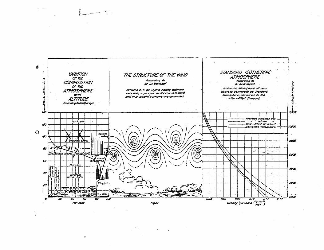
i

0

*
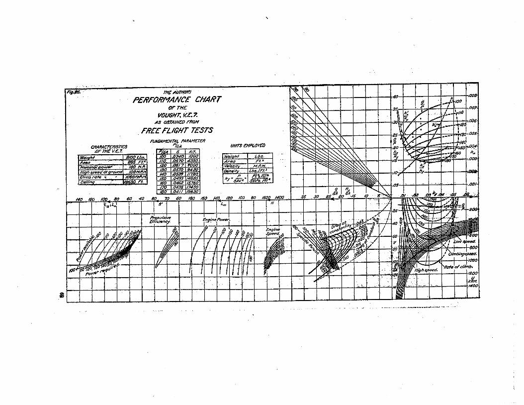