General Revenue Sharing and Public Sector Unions

Laura Feiveson∗

Massachusetts Institute of Technology

December 18, 2012

Abstract

The United States federal government implemented a large general revenue sharing

program from 1972 to 1986, in which it transferred nearly 300 billion (2009) dollars to

over 35,000 state and local governments. I examine whether large city governments

spent the funds that they received and how the strength of public sector bargaining

affected whether the funds were spent on new employment or increased wages. I

find that, on average, city governments spent the transfers completely, in contrast to

the findings of some of the recent "flypaper" literature; and that cities in states with

pro-union collective bargaining laws spent more than half of the transfers on increased

wages while cities in states without such laws spent a greater fraction of the funds on

new employment. These findings suggest that local institutions, in this case public

sector unions, play an important role in determining the way intergovernmental grants

translate into spending outcomes. They highlight the potential heterogeneity in the

way such grants may be spent in different jurisdictions. Moreover, if raising the wages

of existing workers has a different macroeconomic stimulative effect than hiring new

workers, they may also suggest differences across places in the "multiplier" associated

with federal transfers to state and local governments. I find suggestive, though weak,

evidence that the output multiplier on spending on new employment is larger than the

multiplier on increased government wages.

∗I am very grateful to my advisors Jim Poterba and Michael Greenstone for their guidance and support.I also thank Olivier Blanchard, Francesco Giavazzi, Monica Martinez-Bravo, and seminar participants atMIT and SAIS for helpful comments and suggestions.

1 Introduction

In 2012, the federal government transferred more than 600 billion dollars to state and local

governments. Despite the pervasiveness of federal intergovernmental grants, there remains

considerable debate surrounding their use at the local governmental level and their subse-

quent impact on economic activity and the provision of public goods. A relatively unex-

amined possibility is that heterogeneity at the local government level leads to substantial

variation in the response of state and local governments to federal transfers.1 Despite the

focus on labor markets in recent years, the interaction of public sector labor with local gov-

ernment budgeting has generally been neglected in the public finance literature. At the

same time that policy debates surrounding the federal government’s role in alleviating state

and local government fiscal crises have rippled through Washington, protesters and politi-

cians in Wisconsin, Indiana, and Ohio have brought public sector unions to the forefront

of public consciousness. The theoretical underpinnings of research on public sector unions

suggest that there may be a good reason to link the two debates.

In this paper, I seek to address this connection by examining how the strength of public

sector labor unions affects the response of local governments to intergovernmental transfers.

To approach this analysis, I revisit a general revenue sharing program put in place from

1972 to 1986 in which the federal government transferred a total of nearly 300 billion (2009)

dollars to state and local governments. Although the stated goal of the law was to move

the decisions about government spending "closer to the people", it simultaneously helped

to alleviate liquidity crises at the state and local government level during a time period in

which many local governments were facing budget deficits. Furthermore, the passage of

the general revenue sharing legislation came at the end of a fifteen year period in which a

rapid series of new state laws enabled or required local governments to collectively bargain

with their employees. I use the diversity of the collective bargaining laws across states to

examine how the laws affected city governments’use of the intergovernmental transfers and,

in particular, I focus on whether they had influence over whether the transfers were spent on

higher wages for existing employees or on new employment. I present an initial empirical

estimate of the differential impacts on the private economy generated by these different types

of government spending, providing motivation for future research.

The general revenue sharing program is a suitable program with which to study the

effect of intergovernmental transfers on local government expenditure decisions for three

main reasons. First, it significantly impacted the revenues of local governments. At its

1For instance, one well-studied example of a characteristic that has been shown to have significant effectsat the state government level is the stringency of the balanced budget rules (Poterba (1994), Clemens andMiran (2011)).

1

peak, general revenue sharing made up to 20 percent of total revenues of the large city

governments studied in this paper.

Second, there was substantial and plausibly exogenous variation in the amounts that city

governments received. Although the general revenue sharing formula depended on three

factors that would be expected to have a separate effect on government expenditure decisions

(per capita income, tax-to-income ratio, and population), a "geographic tiering" element to

the formula led to variation in the general revenue sharing receipts of city governments that

were housed in different counties and states, but were otherwise very similar. Furthermore,

the three factors entered the allocation formula in highly nonlinear ways, making it possible

to control for them directly. Since the magnitude of transfers to a local government is

often correlated to its economic conditions, it can be diffi cult to disentangle the effects of

the transfers from the effects of the economy. Because of the eccentricities in the formula,

the general revenue sharing program provides variation that is plausibly immune to this

concern.

Finally, the general revenue sharing program led to transfers to over 35,000 state and

local governments including all state, county, city, town and township general-purpose gov-

ernments. It was one of the most comprehensive general purpose transfer programs in the

history of the United States and provides a test case for possible future general revenue

sharing designs.

Although private sector unions were granted full legislative protection in the first half of

the twentieth century, public sector unions did not achieve significant legislative gains until

the late-1950s and 1960s.2 However, starting with Massachusetts in 1958 and Wisconsin

in 1959, a series of state laws were passed in rapid succession. By the time that the State

and Local Fiscal Assistance Act instituted the first wave of general revenue sharing in 1972,

30 states had passed laws enabling or requiring collecting bargaining by local governments

within their state. Figure 1 plots the number of workers and the percent of workers covered

by private and public sector unions from 1977 to 2010. The percent of public sector workers

covered by unions has remained roughly constant at 40 percent for the period shown. The

absolute number of public sector workers covered by unions actually exceeded the number of

private sector workers for the first time in 2009.3 Since public sector collective bargaining

was pervasive by the time that general revenue sharing was put in place, it is possible to

study how the strength of collective bargaining affected the local governments’use of the

2The landmark laws supporting the right to unionize, strike, and collectively bargain in the private sector,i.e. the National Labor Relations act in 1935 and the Taft-Hartley Act in 1947, specifically left out publicsector unions.

3These statistics are from the Survey on Labor-Management Relations in State and Local Governments(U.S. Bureau of the Census, Multiple Years) and www.unionstats.com (Hirsch and Macpherson, 2003).

2

transfers.

The empirical analysis of this paper is organized into three main parts. First, the general

revenue sharing program provides an opportunity to revisit the much-studied research ques-

tion of whether governments used the transfers to increase expenditures or to reduce taxes.

An influential paper by Bradford and Oates (1971) theorized that lump-sum intergovern-

mental transfers should have the same effect on government expenditures as an equivalent

increase in personal income of the voting citizens. An extensive empirical literature has

emerged since this paper, which has found that intergovernmental transfers, at times, lead

to a much higher increase in government expenditures that would plausibly result from an

equivalent rise in personal income. This phenomenon has been dubbed the "flypaper effect"

because the transfer funds appear to stick where they hit.4 The flypaper effect remains

an important policy issue; as the federal government considers transferring funds to local

governments, the question of whether they will spend the funds is crucial to the policy eval-

uation. I find that the large cities I study in this paper increased expenditures by roughly

one dollar for every dollar received in intergovernmental transfers.5

Second, I examine how the strength of public sector collective bargaining laws affects

the expenditure decisions of the recipient governments. Theories of public sector unions

conjecture that union leaders seek to maximize an objective function in which wages and

employment are positive inputs. These theories suggest that bargaining in cities in states

with pro-union bargaining laws may lead to different uses of transfers than in cities in states

with no such laws. I find that the cities with strong collective bargaining laws convert more

of the transfers into increased wages than those with no bargaining laws, and, furthermore,

that those with no bargaining laws instead spent a significant amount of funds on new or

retained employment.

Lastly, I consider one possible implication of these findings. The American Recovery and

Reinvestment Act of 2009 (ARRA) included more than 200 billion dollars of transfers to state

4As summarized by Gramlich (1977) and Hines and Thaler (1995), the empirical literature in the latterhalf of the century had shown the existence of a strong flypaper effect. Explanations of the flypaper effectrange from discussions of a mis-specified model of citizen behavior (see Filimon, Romer and Rosenthal (1982)or Hines and Thaler (1995)) to a repeated game element in the grant process (Chernick (1979)). Inman(2008) provides a comprehensive discussion of other possible explanations. More recent empirical studieshave shown more ambiguous results; the flypaper effect seems to at least crucially depend on factors suchas the type of democracy (Lutz (2006)) and the strength of collective interest groups (Singhal (2008)).Furthermore, Knight (2002) argued that the possible endogeneity of grant assignment due to differentialpreferences for government spending may have led to econometric issues in previous studies, and finds anegligible flypaper effect in transportation grants to state governments when appropriately accounting forlegislative bargaining power.

5Because the general revenue sharing program did include some minor price effects, they were not purelump sum transfers and thus do not directly address the traditional flypaper effect. Details of the generalrevenue sharing program and how they relate to the flypaper effect will be discussed in Sections 2 and 6.2.

3

and local governments. The magnitude of this component of the stimulus component has

led to a renewed interest in the estimation of the government spending multipliers associated

with intergovernmental transfers.6 My results suggest that public sector unions may be a

factor in the determination of the size of these multipliers. Starting with Wynne (1992), a

distinction in the theoretical and empirical literature has been made between the stimulative

effects on the private economy of government consumption of private goods and government

compensation of employees.7 A similar distinction can be made between government spend-

ing on increased government wages and increased government employment, due to differential

marginal propensities to consume between the two types of recipient employees. Because the

strength of collective bargaining laws determines the type of government spending produced,

I use this institutional friction to explore the hypothesis that the multipliers on spending on

increased wages and on spending on new employment would be different. I find suggestive,

though weak, evidence that the multiplier on increased government employment is larger

than the multiplier on increased government wages for existing employees. These results

are presented as motivation for future research.

The paper is organized as follows: Section II discusses the framework for the analysis.

Section III reviews the program details of the general revenue sharing transfers, Section IV

introduces the empirical strategy, Section V explains the data that are used, and Section

VI discusses the main results. Section VII introduces the macroeconomic hypothesis and

empirical analysis. Finally, Section VIII concludes.

2 Framework

In this section, I consider how the public sector unions might seek to influence the use of

intergovernmental transfers at the local government level. The standard consensus is that

the public sector union has a utility function over wages and employment, increasing in both

(Dunlop (1944), Farber (1986)).8 The intuition of why wages are in the utility function is

clear; we generally think that an increase in income, given the same amount of work, yields

6A number of studies have directly estimated the multipliers associated with this component of the ARRA:Chodorow-Reich et al (2012), Cogan and Taylor (2011), Conley and Dupor (2012).

7See Finn (1998), Pappa (2009), and Ramey (2011).8This is a simplification of a very large literature. Starting with Ross (1948), there has been debate

over the value of assigning a well-defined utility function to the labor representation. In particular, politicalmotivations of union leadership and heterogeneous membership make the objectives diffi cult to summarize.Ashenfelter and Johnson (1969) propose an alternative bargaining model in which there are three parties:the firm management, the union leadership, and the union “rank and file”. In this spirit, many recent papersstress the political motivation of the union leadership in their models of union behavior.

4

an increase in utility.9 However, the idea that the union leadership would also value higher

levels of employment is less obvious.10 The theories that advocate for having employment

in the utility function mostly rely on the idea that higher levels of employment increase the

negotiating power of the public sector union members. In addition, some economists have

argued that public sector unions put greater weight on employment than private sector unions

because numbers boost the ability of the union to sway elections (Courant, Gramlich, and

Rubinfeld (1979), Freeman (1986)). On the other hand, advocates of the "insider-outsider"

theory conjecture that the current members care only about their own wages and job security

without any direct desire to increase employment (Blanchard and Summers 1986).11 Finally,

it is worth pointing out that the objective functions of public sector unions may include

more than just wages, employment, or personal benefits; in particular, because public sector

employees have influence over the provision of public goods, they may also include the welfare

of citizens in their utility function. For example, one reason that public sector unions may

lobby for more public funds is that they have an in-depth understanding of how to supply

services in the most effective way (Zax and Ichniowski 1988).

Motivated by these considerations about the union’s objectives, the intergovernmental

grant utilization decision that I particularly focus on is whether the transfer funds are spent

on wages, w, or new employment, E. In my stylized world, all local government expenditures

are on labor such that the relationship between E and w is constrained by the allotted local

government budget, B, satisfying the budget constraint, B = wE. When a grant is received

by a local government, the flypaper effect leads to an outward shift in this labor demand

curve, such that B′ = B+µfT = wE, where µf is the percent of the transfers that is retained

by the government rather than returned to the taxpayers in the form of reduced taxes.12 On

the labor supply side, I assume that the union can choose the point on the labor demand

curve that maximizes their objective function. The left panel of Figure 2 shows one possible

9Empirical evidence has shown that there is a significant union-nonunion public sector wage gap. SeeLewis (1990), Zax and Ichniowski (1988), Hoxby (1996), and Frandsen (2011).10The empirical evidence is also mixed. While Zax and Ichniowski (1988) found a significant effect of

unionization on employment, others have found that omitted variables may have biased naive regressions ofemployment on unionization. Trejo (1991) argued that economies of scale led to more union formation inlarger municipalities, leading to a natural correlation between unionization and employment that could bedeceptively interpreted causally. Valletta (1993) argued that municipalities with high levels of volunteerismor privatization tend to have fewer unions and smaller governments.11By limiting the discussion of the objective function to only employment or wages, I am skimming over

other variables that have been included in the utility functions of unions. For instance, in the utility functionposited by Blanchard, Summers (1986), the union members valued wages and the probability of retainingtheir job in the next period. It is also worth mentioning that their model surrounds the private sector ratherthan the public sector.12It is important to note that µf may itself be effected by the extent of unionization, a possibility that I

explore in the empirical analysis.

5

outcome when the supply curve is shifted outward in which both employment and wages

increase.13 In the other extreme, the governments that are not subject to strong unions

instead face competitive wages for government workers. Thus, the labor demand curve is

flat, and any expansion in the budget has no effect on wages and is used directly to increase

government employment as demonstrated in the right side of Figure 2.

Obviously, these are extreme cases and I write them only to illustrate how public sector

unions may lead to a different utilization of transfers than what would occur in their absence.

The mechanism I describe above implicitly assumes that the public sector union is aware of

and able to bargain over the change in the budget to reach their optimal point on the budget

curve. This assumption might break down for other shifts to the budget such as business

cycle related changes to tax revenue. Since intergovernmental transfers are announced and

have a very specific timing attached to them, their arrival is a concrete item over which to

bargain. As the events of 2011 and 2012 in many of the Midwestern states have proved,

public sector unions are strong forces at the bargaining table, and it is likely that they will

influence the use of transfers in the ways I stylized above even if they are unable to influence

the response to other more intangible income shocks.14

3 General Revenue Sharing

The policy debates surrounding the growing roles of local governments in the late 1960s and

early 1970s ultimately led to the passage of the State and Local Fiscal Assistance Act in

October of 1972. This act put in place the largest general revenue sharing scheme in the

history of the United States. With this policy, the federal government initially committed

to transferring over 30 billion dollars to more than 35,000 general purpose governments—

state, county, city, town, and township governments—over a period of 4 years. In 1976,

the act was extended for another period of 4 years for state and local governments, and

then extended for only local governments from 1980 to 1983 and again from 1983 to 1986

when it finally expired. By the end of the act, over 83 billion dollars (almost 300 billion

in 2009 dollars) had been transferred to state and local governments. The motivations for

13Certainly utility functions exist such that the unions would choose to decrease either wages or employ-ment when the budget is increased, if the cross partials are negative. However, I think it is completelyreasonable to assume that, at the very least, political economy constraints would ensure that wages andemployment both weakly increase when there is an expanded budget. The purposes of this graph are to beillustrative and I leave it to the empirics to be exact about what would actually happen.14Relatedly, Allen (1998) address the question of how public sector unions affect employment in the

presence of negative revenue shocks. Because of the reasons just outlined above, this question does notdirectly relate to the questions that I address in this paper. He finds that, contrasting with the dymanicsin the private sector, union workers in the public sector face lower rates of unemployment than nonunionworkers when faced with revenue losses.

6

the act were both philosophical and practical; the offi cial goal was to have decisions about

government spending "closer to the people", while the act simultaneously served the purpose

of providing support to local governments at a time in which many budgets were strained.

Although some evidence implies that the Nixon administration had the intention of using the

general revenue sharing funds to replace various federal categorical grant programs to local

governments, in practice, it acted as a supplement to the programs that already existed.15

The most binding requirement surrounding the use of the funds was that they were not to be

used for operational education expenses; no general revenue sharing funds were transferred

to school districts. Otherwise, the governments had almost complete freedom to use the

funds as they desired.16 The governments did have to fill out a "statement of use" in which

they described how they used the funds.17 Furthermore, after the first extension of the

funds, the local governments were required to hold public hearings in which the potential

uses of the funds were discussed.

Table 1 shows the size of the program throughout the 14 years of its existence. At the

peak of the program’s impact, in 1974, general revenue sharing (GRS) made up about 15

percent of total federal intergovernmental transfers to state and local governments, and com-

posed almost 3 percent of state government budgets and over 3.5 percent of local government

budgets. As Table 1 shows clearly, the size of the program in real dollars decreased sub-

stantially over its tenure due to relatively high inflation in the 1970s and the 1980s combined

with stagnant nominal amounts. By 1984, the program only amounted to 0.12 percent of

GDP and less than 2 percent of local government budgets. Despite the ramp-down, the

general revenue sharing program had a substantial effect on the revenues of the 837 cities in

my sample. Figure 3 plots both the total federal intergovernmental funds as well as the total

general revenue sharing funds received by the city governments. The figure demonstrates

15In fact, the Nixon administration promised that the general revenue sharing program would be an "add-on" to existing programs in order to get the support for the passage of the act (Dommel, 1974). However, afterthe act was passed and Nixon was re-elected in 1972, the administration began to push for the elimination ofmany block grant programs, claiming that the general revenue sharing funds would make up for the reducedtransfers. The Watergate scandal ultimately interfered with the implementation of this policy push, and thegrant programs remained largely unscathed, reinforcing the "add-on" nature of the general revenue sharingprogram (Markusen et al, 1981).16Specifically, the "priority" categories on which the funds could be spent were: all "ordinary and nec-

essary" capital expenditures, and "ordinary and necessary" maintenance and operating expenses for publicsafety, environmental protection (including sewerage and sanitation), public transportation, health, recre-ation, libraries, social services for the poor or aged, and financial administration (Joint Committee on InternalRevenue Taxation, 1973). In practice, the only major binding requirement was that the funds were not tobe used for education operating expenses.17The specific requirements were the the funds had to be appropriated within 24 months of the entitlement

period. Local governments had to fill out planned use and actual use reports and make them available tothe public. The planned use reports were to be filled out within each entitlement period while the actualuse reports were to be filled out within 60 days of June 30th of each year.

7

that the movements in total federal intergovernmental transfers appeared to reflect the jump

in general revenue sharing funds in the early-1970s as well as the ramp-down in the early-

to mid- 1980s.

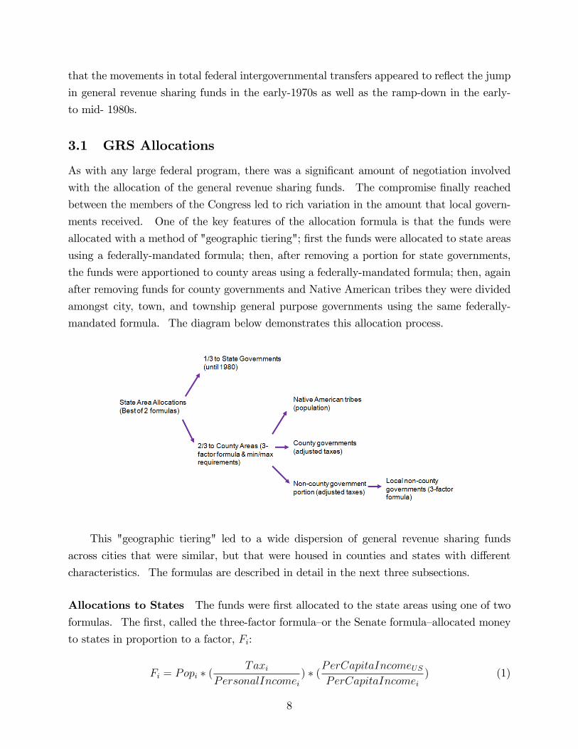
3.1 GRS Allocations

As with any large federal program, there was a significant amount of negotiation involved

with the allocation of the general revenue sharing funds. The compromise finally reached

between the members of the Congress led to rich variation in the amount that local govern-

ments received. One of the key features of the allocation formula is that the funds were

allocated with a method of "geographic tiering"; first the funds were allocated to state areas

using a federally-mandated formula; then, after removing a portion for state governments,

the funds were apportioned to county areas using a federally-mandated formula; then, again

after removing funds for county governments and Native American tribes they were divided

amongst city, town, and township general purpose governments using the same federally-

mandated formula. The diagram below demonstrates this allocation process.

This "geographic tiering" led to a wide dispersion of general revenue sharing funds

across cities that were similar, but that were housed in counties and states with different

characteristics. The formulas are described in detail in the next three subsections.

Allocations to States The funds were first allocated to the state areas using one of two

formulas. The first, called the three-factor formula—or the Senate formula—allocated money

to states in proportion to a factor, Fi:

Fi = Popi ∗ (Taxi

PersonalIncomei) ∗ (PerCapitaIncomeUS

PerCapitaIncomei) (1)

8

The first term of this factor was geared towards equalizing the per capita funds transferred

to states. The second component was to address the concern that states may lower taxes

in response to the increased federal funds; to try to reduce the incentives to do this, high

taxation rates were rewarded. Finally, the third term transferred more funds to states that

had lower per capita income. Under this allocation formula, each state i was awarded, S1i :

S1i = G ∗ ( Fi∑States

Fk) (2)

where G was the total amount of general revenue sharing funds available for distribution.

In the second, five-factor (House) formula, the allocation was divided into five parts which

were each distributed using a different formula as shown in the table below:

Fraction of Funds Factor used for Allocation

0.25 Popi

0.25 UrbanPopi

0.25 Popi ∗ (PerCapitaIncomeUSPerCapitaIncomei)

0.125 IncomeTaxi

0.125 Taxi ∗ ( TaxiPersonalIncomei

)

Under this formula, the total GRS allocation was divided into parts and then distributed

according to the factors discussed in the table above. Each state was awarded S2i :

S2i = G ∗

0.25 ∗ Popi∑States

Popk+

0.25 ∗ UrbanPopi∑UrbanPopk

+

0.25 ∗Popi

PerCapitaIncomei∑ PopkPerCapitaIncomek

+

0.125 ∗ IncomeTaxi∑IncomeTaxk

+

0.125 ∗Tax2i

PerCapitaIncomei∑ Tax2k

PerCapitaIncomek

(3)

The final allocation was reached by first calculating the distribution of funds, S1i and

S2i , for all of the states under each of the three-factor and the five-factor formulas, and

then taking the larger of the two amounts for each state. These final amounts were then

proportionately adjusted so that the total amount summed to the total GRS funds available.

The final allocation for each state area was then:

SFi = G ∗ max(S1i , S2i )∑

max(S1k , S2k)

(4)

9

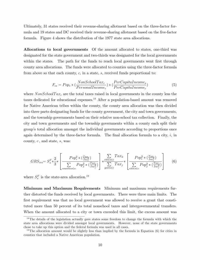
Ultimately, 31 states received their revenue-sharing allotment based on the three-factor for-

mula and 19 states and DC received their revenue-sharing allotment based on the five-factor

formula. Figure 4 shows the distribution of the 1977 state area allocations.

Allocations to local governments Of the amount allocated to states, one-third was

designated for the state government and two-thirds was designated for the local governments

within the states. The path for the funds to reach local governments went first through

county area allocations. The funds were allocated to counties using the three-factor formula

from above so that each county, c, in a state, s, received funds proportional to:

Fcs = Popc ∗ (NonSchoolTaxcPersonalIncomec

) ∗ (PerCapitaIncomesPerCapitaIncomec

) (5)

where NonSchoolTaxc are the total taxes raised in local governments in the county less the

taxes dedicated for educational expenses.18 After a population-based amount was removed

for Native American tribes within the county, the county area allocation was then divided

into three parts designating funds for the county government, the city and town governments,

and the township governments based on their relative non-school tax collection. Finally, the

city and town governments and the township governments within a county each split their

group’s total allocation amongst the individual governments according to proportions once

again determined by the three-factor formula. The final allocation formula to a city, i, in

county, c , and state, s, was:

GRSics= SFs ∗2

3∗

Pop2c ∗ (TaxcInc2c)∑

counties∈sPop2j ∗ (

TaxjInc2j

)

∗∑

cities∈cTaxk∑

govts∈cTaxj

∗

Pop2i ∗ (TaxiInc2i)∑

cities∈cPop2j ∗ (

TaxjInc2j

)

(6)

where SFs is the state-area allocation.19

Minimum and Maximum Requirements Minimum and maximum requirements fur-

ther distorted the funds received by local governments. There were three main limits. The

first requirement was that no local government was allowed to receive a grant that consti-

tuted more than 50 percent of its total nonschool taxes and intergovernmental transfers.

When the amount allocated to a city or town exceeded this limit, the excess amount was

18The details of the legislation actually gave states some freedom to change the formula with which thestate area allocations were divided amongst local governments. However, none of the state governmentschose to take up this option and the federal formula was used in all cases.19The allocation amount would be slightly less than implied by the formula in Equation (6) for cities in

counties that included a Native American population.

10

reallocated to the corresponding county government. When the amount allocated to the

county government exceeded this amount, the funds went back to the state government.

Because of this restriction, more than 10 state governments received more than one-third of

their state’s allocation, with West Virginia, Kentucky, and Delaware receiving substantially

more than the one-third initially allocated (45%, 41%, and 40% respectively).

The second limit was that no county area or local government was permitted to receive

more than 145 percent of the state per capita amount, and the third limit was that no

county area or local government was permitted to receive less than 20% of the state per

capita amount. At the county area level, those funds that were in excess of the 145 percent

limit were distributed to the non-binding county areas proportionate to the three-factor

formula. Similarly, funds were reduced proportionately in non-binding county areas to meet

the 20 percent limit for those areas that needed extra funds. Similar adjustments occurred

for those local governments that were constrained at the 20 percent or the 145 percent limits.

To be clear, I will map out the steps in which city governments were received funds from

their county-wide allocations. Suppose that a county area received GRS0c through the

allocation process. A city government, i, within the county would initially receive20:

GRS0i = (Popi∗( NonSchoolTaxi

PersonalIncome1969i) ∗ (PerCapitaIncomei

PerCapitaIncomec)∑

cities

Popj∗(NonSchoolTaxj

PersonalIncome1969j) ∗ (PerCapitaIncomej

PerCapitaIncomec))

∗GRSc∗(

∑Ci ties

NonSchoolTaxk∑GovernmentsInCounty

NonSchoolTaxj) (7)

The first additional requirement was that the city government did not receive more than fifty

percent of its total nonschool taxes and intergovernmental transfers. Thus, in the second

step of the allocation, the city government received GRS1i:

GRS1i = min (GRS0i, 0.5 ∗ (NonSchoolTaxi + IGRi)) (8)

Any excess amounts generated in this step, GRS0i − GRS1i, were assigned to the county

governments within the county. The second and third limits were then applied such that:

GRS2i = min

(max

(GRS1i, 0.2 ∗ (

GRSsPops

)

), 1.45 ∗ (GRSs

Pops)

)(9)

20If there were Native American Tribes in the county, a portion of GRSc would be removed before theallocation in Equation (6).

11

Any excess amounts generated in this step, GRS1i−GRS2i, were added to the initial county-wide allocation, GRSc, and any shortage of funds generated, GRS2i−GRS1i were subtractedfrom GRSc. At this point, the steps represented in Equations (7) - (9) would be repeated

again until all binding requirements were met.21 Note that, due to the iteration of these

steps, the maximum and minimum requirements ended up affecting the allocations of gov-

ernments that were not at the limits of the requirements. In the first year of the GRS

program, 6.6 percent of the GRS funds were redistributed through limits and only 74 out of

the 38,000 recipients had allocations which were unaffected by the limit requirements.

3.2 Variation in GRS receipts

Any examination of the GRS aggregates will mask the significant variation in the per capita

funds received by local governments due to the geographic tiering and other nuances of the

allocation process. The variation is especially large at the city level, which is the unit of

observation in this paper. To give a sense of the variation, in Figure 5, I plot a histogram of

the de-meaned per capita general revenue sharing transfers in 1977. Although the variation

in Figures 5 is useful to observe, the variation that I will use in future regressions is the

residual left once I control for smooth functions of all of the variables that appear in the

allocation formulas in Equations (1) - (9). Figure 6 shows the residuals from a regression

of per capita general revenue sharing receipts on cubic polynomials of all of the allocation

variables in 1977.22 Due to the geographic tiering and the non-linearity of the allocation

formulas, this figure shows that substantial cross-sectional variation in the general revenue

sharing funds remain even after controlling for flexible functions of the allocation variables.

4 Empirical Strategy

I estimate how cities respond to intergovernmental transfers, and how the strength of public

sector collective bargaining affects that response. The main estimation equation is:

Eit = β0 + β1IGRit + β2IGRit ∗ Uit + β3Uit +Xitη + λi + ωt + εit (10)

where Eit is a per capita government finance component in government i and year t, IGRitare the per capita intergovernmental transfers, Uit is an indicator for the strength of collective

bargaining laws, λi are city fixed effects, and ωt are time fixed effects. Xit is a set of control

21If, at any step, the amount allocated to the county government exceeded 50 percent of the sum of itsnonschool taxes and intergovernmental transfers, the excess would be allocated to the state government.22The detailed list of controls will be discussed in Section 5.7.

12

variables including cubic polynomials of population, lagged per capita tax revenue, lagged

tax effort, lagged own-source revenue, lagged per capita county income, lagged state-level

total taxes, lagged state per capita income, and lagged state government individual income

taxes. Although I show the results for a number of finance components, the outcome

variables that I particularly focus on are total real expenditures, public employee real wages,

and the number of public employees. The effect of the transfers on total expenditures will

demonstrate whether governments spend the funds transferred to them (i.e. the expenditure

effect), while the latter two outcome variables will speak to the quality of the public spending.

Later in the paper, I discuss how the quality of public spending might impact the stimulative

effectiveness of transfers to city governments, particularly during recessions.

An issue with the estimation of Equation (10) is that the federal and state governments

target some of their funds to cities or areas that are in particular need. This could bias β1and β2 either downward or upward if there is a systematic difference in how city governments

"in need" and other cities respond to the transfers. For example, if funds are transferred

to cities with high unemployment, reversion to the mean may mistakenly attribute an im-

provement in economic conditions (and thus an increase in government expenditures) to the

transfers received. On the other hand, if funds are transferred to cities that are beginning

to experience budgetary problems, the continuation of the negative trend (leading to a con-

traction in government expenditure) may be wrongly attributed to the transfers, biasing the

β coeffi cient downwards.

4.1 A 2SLS Approach

To address the problem of potential bias, I use the general revenue sharing transfers as an

instrument for total intergovernmental transfers. In particular, I have two instruments,

GRSit, per capita general revenue sharing receipts, and GRSit ∗ Uit, per capita generalrevenue sharing receipts interacted with the indicator for bargaining strength, for the two

endogenous variables, IGRit and IGRit ∗ Uit. Because I control for the cubic polynomials

of all of the GRS-correlated variables, my instruments are essentially the GRSit and the

GRSit ∗ Uit after conditioning for these variables. I estimate using 2SLS estimation, in

which the second stage is represented by Equation (10), and the two first-stage regressions

are:

IGRit = ϕA0 + ϕA1GRSit + ϕA2GRSit ∗ Uit + ϕA3 Uit +XitαA + σAi + µAt + νAit (11)

13

IGRit ∗ Uit = ϕB0 + ϕB1 GRSit + ϕB2 GRSit ∗ Uit + ϕB3 Uit +XitαB + σBi + µBt + νBit (12)

The exclusion restriction of the IV estimation is that GRSit and GRSit ∗ Uit are in-dependent of the error term in Equation (10). As described above, the nonlinearities in

the general revenue sharing formula ensured that similar cities received different amounts

of funds. However, the three-factor and five-factor formulas imply that the GRS transfers

were correlated to per capita income, non-school "tax effort", and population of the city

governments, as well as the higher-level variables used for the allocation to their encompass-

ing counties and states. Assuming that the expenditures are independent of all of these

variables would be implausible; in particular, the city-level tax effort, taxes and population

as well as the county-level per capita income seem likely to have an effect on city government

expenditure decisions in perhaps a nonlinear way.23 To satisfy the exclusion restriction given

my assumptions, I include a flexible cubic polynomial of the lags of each of the variables that

are used in the general revenue sharing calculation.24 Details on the sources of the controls

are described in the next section.

Given the independence of GRSit, I argue that GRSit∗Uit is also independent of the errorterm in Equation (10). Since most of the law changes to Uit occurred before the estimation

time period, the city fixed effects will largely pick up the city characteristics that may have

been correlated to Uit. However, there is a concern that the controls included to ensure the

independence of the GRSit, i.e. the city-level tax effort, taxes, and population, and county

income, may affect "no-bargaining" cities in a different way than "bargaining" cities. To

account for this possibility, I also interact each control with the bargaining indicator, Uit, in

my preferred specification.

Finally, for those cities that were parts of states that instituted bargaining laws within

the sample studied, there is the concern that factors present within the cities (and reflected

in city government finance decisions) affected the timing of the passage of the laws. If this

were the case, than it is possible that Uit is correlated with εit in Equation (10). As is

shown in Figure 8, 8 states passed laws during the period studied, changing their value of

Uit. Extensive research on the collective bargaining laws carried out in the late 1980s found23Because the city-level per capita personal income is only released every 10 years, the (annual) county-

level per capita income is the variable in the GRS formula that best proxies fluctuations in local-area personalincome.24The general revenue sharing allocations were updated quarterly with the most current data available.

In practice, this meant that the data used in the GRS formula were lagged at least 2 to 4 quarters. To bestapproximate this lag with annual variables, I include all controls with a one-year lag. Furthermore, I do notinclude county-level controls or the state-level urban population, since these variables were not updated onan annual basis.

14

that, given that the change was ultimately going to occur, the timing of the law passages

were largely exogenous, having more to do with the superficial political environment of the

state legislature than the political or public will towards collective bargaining. Ohio is a

good example of this; although Ohio had some of the strongest private sector unions in the

country, they were one of the last states to pass a public sector bargaining law in 1985.

Although the will of labor and the public had been behind the law for many years, haggling

over the details of the law lead to a long delay. Saltzman (1988) documents this delay,

and also argues convincingly that the passage of the law in Ohio had a significant effect on

the strength of its public sector unions. Freeman and Valletta (1988) also provide evidence

that the state laws were a major factor in determining whether public sector employees were

covered by collective bargaining contracts. Given this research surrounding the timing of

the laws, it may be reasonable to assume that the city fixed effects will pick up any political

or public will toward collective bargaining so that the timing of the law change and Uit, and

GRSit ∗ Uit, remain independent of the error term.

4.2 Further Assumptions

To ensure the validity of the empirical strategy outlined above, I must make two more

assumptions. First, I assume that the dependent varible in Equation (10) depends only on

contemporaneous general revenue sharing funds, and not on lagged or future general revenue

sharing funds. Since GRSit can affect future values of itself through macroeconomic effects

on Iit or any of the other correlates, changes to GRSit may be correlated over time. By

only including the contemporaneous change, I introduce an omitted variables problem if the

true relationship actually consisted of the dependent variables depending on future or past

values of GRSit. I test this by including past and future values of GRSit in the estimation

equation. I find that the results are little changed, although the standard errors increase.

Second, I assume that the coeffi cients on GRS-correlated cubic controls are constant over

time. This would not be true, for example, if different governors or mayors weigh personal

income differently when determining budgeting policies. If the coeffi cients are not constant

over time, the cubic controls as described in Section 4.1 would not appropriately account

for that portion of the general revenue sharing variation that was due to fluctuations in its

correlates. To deal with this possibility, in a robustness check, I interacted all of the controls

with year dummies and include them in the main specification. I find that the direction of

the main results are little changed. In my preferred specification, however, I do not include

the control-time interactions.

Further robustness measures are reported in Section 6.

15

5 Data

In this section, I describe the sample used for the analysis, the data sources, and the summary

statistics. In the appendix, I include an additional explanation of the adjustment I make to

account for the variation in the fiscal years covered by the Annual Survey of Governments.

5.1 The Sample

State and local governments are often under-emphasized in analyses of the government spend-

ing in the United States. In the 2000s, federal nondefense consumption and investment made

up only about 2 percent of GDP in comparison to that of state governments which made

up 4 percent of GDP and that of local governments which comprised 8 percent of GDP.25

Federal defense spending is more volatile, making up more than 10 percent of GDP in the

1960s and less than 4 percent of GDP at its trough in 2000. Figure 7 shows this breakdown

of government spending and highlights the particular importance of local governments to

GDP.

Despite its limited direct effect on GDP, federal policy does play a significant role in the

path of government consumption and investment through its control over intergovernmental

grants to state and local governments as well as regulation of their activities. In this

paper, I focus on the effect of intergovernmental grants to large city governments over the

period 1971 to 1989. This time period comes at the tail end of a fifteen-year period of

rapid growth in local governments; as seen in Figure 7, the local government contribution

to GDP grew from 5.9 percent in 1959 to 8.2 percent by 1974 after which it roughly leveled

off. I specifically focus on city governments that had a population of 25,000 or greater in

1972. Collectively, these 837 city governments accounted for roughly 30 percent of all local

government expenditure.26

City governments provide a broad range of services including police and fire protection,

highway construction, sewerage, solid waste management, and utility provision. Their

revenues come mainly from a combination of property taxes, intergovernmental revenues,

charges and fees, and utility payments. Table 2 shows the breakdown of expenditures and

revenues for the 837 cities studied in this paper.

25Each of these estimates came from averaging over the years 2000-2007, which are the seven most recentyears in which the government GDP data were broken up between state and local governments. During thesame time period, federal defense consumption and investment made up 4.4 percent of GDP. All componentsof government together made up 18.6 percent of GDP.26In 1972, the number of governments (with the percent of the local government expenditure that they

made up in parentheses) was: 3044 county governments (20%), 18,517 city and town governments (36%),16,991 township governments (3%), 23,885 special district governments (7%), and 15,779 school districts(33%).

16

It is worth noting that although education expenditures made up 13 percent of the total

expenditures of all of the cities in the sample (see Column (2) of Table 2), less than half of

the cities have a positive amount of education expenditures (Column (3) of Table 2). In fact,

only 131 of the city governments in the sample are responsible for the K-12 school systems

within their city. In the other 706 cities, school districts with separate revenue streams are

responsible for funding and organizing K-12 education. When including school districts in

the universe of all city, town, and township governments, education made up more than 50

percent of total expenditures in 1977.

5.2 The Annual Survey of Governments

Since many of the variables used in the estimation are directly from the Annual Survey of

Governments (ASG) produced by the Bureau of the Census, it is worth mentioning a few

facts about this survey. In years ending in -2 and -5, the Census conducts a complete

survey of all state, county, city, town, and township governments and school districts. In

the intermediate years, they only survey a random sample in which local governments are

assigned a probability depending on the area population and other characteristics. Because

most large cities are included in the yearly sample with 100% probability, most of the cities

in my sample are represented in every year from 1971-1989.27 The exact variables used from

the survey will be described in the sections below. All of the finance variables used from

the ASG are deflated using the state and local GDP deflator (from the Bureau of Economic

Analysis) and are normalized by the city population (from the ASG).

5.3 Outcome Variables

The three outcome variables that I will focus on are total city government expenditures,

normalized employment, and normalized government employee annual wages. Total expen-

ditures come directly from the ASG and are deflated using the state and local GDP deflator

and normalized by the city population. To calculated normalized annual wages, the an-

nual wages are first computed by dividing deflated salaries and wages by total government

employment. Multiplying this annual wage by the number of government employees in

1972 gives the normalized wage. The normalized employment variable is arrived at in a

similar manner, from multiplying total government employment by the 1972 annual wage.

The purpose of these normalizations is to convert the employment and wage variables into

27The sample consists of 837 cities that had a population of greater than 25,000 in 1972. All of the citiesappear in the sample for the following years: 1972, 1974, 1975, 1976, 1977, 1978, and 1979. For the rest ofthe years, the number of cities in the sample is shown in parentheses: 1971 (806), 1973 (805), 1980 (834),1981 (835), 1982 (830), 1983 (830), 1984 (830), 1985 (829), 1986 (829), 1987 (830), 1988 (828), 1989 (803).

17

expenditure statistics such that the β1 and β2 coeffi cients in Equation (10) can be used

to answer the question: How much of each dollar transferred to local governments goes

towards employment, and how much goes toward increased wages? I use these normalized

variables for ease of interpretation; the message and significance are unchanged when I use

non-normalized employment and annual wages in the estimations.

I show results for other outcome variables. Capital outlays, expenditures on employee

retirement programs, and own source revenues are taken directly from the ASG. Net new

debt issued is calculated by subtracting retired debt from new debt issues, the change in

cash and security holdings is calculated from subtracting the previous year’s holdings from

the current year holdings, and the change in retirement fund cash and security holdings is

also calculated by subtracting a lag of total holdings from the holdings in the current year.

5.4 Union Variables

The variables used to represent the collective bargaining strength of the public sector come

from a dataset collected by Richard Freeman and Robert Valletta at the National Bureau of

Economic Research for the years 1959 to 1986, and then extended by Kim Rueben through

1996. In my preferred specification, I use an indicator variable that is equal to zero if the

city resides in a state in which there is no provision for public sector collective bargaining or

in which collective bargaining is explicitly prohibited. In the cities that reside in a state with

an indicator of one, it is either the case that there is a "weak" bargaining provision in which

public sector labor has a right to present proposals or to meet and confer or the employer

is authorized but not required to bargain, or a "strong" bargaining provision in which the

public sector employers have an implied or explicit duty to bargain "in good faith". Figure

8 shows the timing of the legislation passage for this indicator variable.

Figure 9 shows the geographic variation across states in the collective bargaining laws in

the year 1972. Expectedly, there appears to be a high correlation between the existence of

collective bargaining laws and the party preference of a state. In the robustness section, I

will show that controlling for the party of the state governor does not alter the estimated

effects of the collective bargaining indicator term.

The Freeman-Valletta dataset and the Rueben extension distinguish between bargaining

laws for state employees, municipal police, municipal fire fighters, noncollege teachers, and

other local employees. I use the "other local employees" category for the creation of the

union indicator variable. The correlation between the legislation for different employee

groups is high.28

28Over the time period 1970 to 1989, the correlation between the indicator representing a weak bargainingprovision for "other local employees" and each of the indicators for police employees and fire protection

18

In the robustness section, I explore the results with two different possible union variables.

First, I examine an indicator as to whether union dues are allowed to be subtracted directly

from the paychecks of government employees. Second, I create an indicator which represents

whether there exists legislation which specifically includes wages in the scope of bargaining.

5.5 Endogenous Variables

In all of the instrumental variable regressions, the two endogenous variables are per capita

intergovernmental transfers and per capita intergovernmental transfers interacted with the

union variable described above.29 Intergovernmental transfers are from the ASG.

5.6 Instruments

The two instruments used are the general revenue transfers received by the city, and the

general revenue sharing funds interacted with the union variable. Because the ASG included

a general revenue sharing variable for the years in which the program was in place, I have

the exact amounts that the city governments received through the program (as reported in

the Census survey by the city governments).

5.7 Controls

In almost all regressions, I include city and year fixed effects. Because of this, any city

characteristics that are immutable over time cannot be included in the regressions as they

are collinear with the government fixed-effects. The baseline controls that I choose to use

are those that validate the instrument, as discussed in Section 4.1. The controls that I use

are a flexible cubic polynomial in each of the following variables: population, lagged per

capita tax revenue, lagged "tax effort" (non-school taxes divided by 1969 per capita personal

income), lagged per capita county income, lagged state-level total taxes, lagged state per

capita income, and lagged state government individual income taxes.30 Tax revenue is from

the ASG, 1969 per capita personal income is from the 1970 Dicennial Census, and county

personal income is from the Bureau of Economic Analysis (BEA) regional accounts. I

employees is greater than 70 percent. The correlation with the bargaining provisions for noncollege teachers(which is less relevant for the study of general revenue sharing) is 50 percent.29I choose total intergovernmental transfers rather than just federal intergovernmental transfers because

of a correlation between general revenue sharing funds and state intergovernmental transfers. The sourceof this correlation is described in Section 6.1.30For areas smaller than counties, per capita income is released every ten years as a part of the Decennial

Census. The measure of local per capita income used in the general revenue sharing formulas through 1982was therefore the 1969 per capita income published in the 1970 Decennial Census.

19

also include a cubic polynomial of lagged own source revenue as a baseline control variable.

Although the GRS formula relied on own source taxes, there is evidence that some of the

local governments were able to count other types of revenue (fees, for example) in the tax

base when the formula was calculated. To fully capture this, I include total own-source

revenues as a control.

5.8 Summary Statistics

Table 3 shows the summary statistics for the variables used in the estimation equations

for the year 1977. On average, cities employeed over 2,000 workers and paid them almost

37,000 (2005) dollars each, although the variation across cities for both of these statistics

was substantial. The average city population in my sample was about 100,000, again with

considerable variation.

6 Results

In this section, I present the baseline results. I first show that the IV regressions have a

strong first-stage. I then examine the flypaper effect and find that the city governments

increased expenditures by one dollar for every dollar of intergovernmental transfers received.

In the next subsection, I explore what the city governments spent the funds on; in particu-

lar I examine the employment/wage decision and find that the no-bargaining cities used a

significant portion of the transfers to fund new employment whereas the bargaining cities

spent on increased wages instead. Finally, I explore the robustness of the results.

6.1 First-Stage Regressions

Table 4 displays the first-stage regressions in specifications that do not yet include the

indicator for bargaining. The first three columns of Table 4 show OLS regressions of per

capita intergovernmental transfers against per capita general revenue sharing receipts, as well

as a set of controls including city fixed effects, year fixed effects, and state-time trends. In

the first column, I include the full set of baseline controls (without the interactions with the

bargaining indicator), in the second column, I exclude the quadratic and cubic polynomials

of the allocation variables, and in the third column I do not weight by population. Columns

(4) and (5) split the effect on total intergovernmental transfers into the effect on federal

intergovernmental transfers in Column (4) and state intergovernmental transfers in Column

(5).

20

The first-stage is strong. The coeffi cient of 1.5 in Column (1) implies that each dollar

of per capita general revenue sharing receipts to the city governments led to an increase

in per capita intergovernmental transfers of 1.5 dollars. There are two main reasons that

the coeffi cient exceeds one. First, as shown in Column (5), a large part of the excess

is due to a positive (albeit insignificant) correlation between the general revenue sharing

transfers and state intergovernmental transfers. Because the geographic tiering led to a

high correlation between the state government general revenue sharing funds and the local

government general revenue sharing funds, one would expect that the state intergovernmental

transfers would be correlated with the city general revenue sharing receipts if the state

governments "passed on" a certain percentage of revenue that they received from the federal

government. Furthermore, it is possible that state governments piggy-backed on the general

revenue sharing formula to disperse some of their own intergovernmental transfers, which

would also lead to a positive coeffi cient in Column (5). The positive correlation between

the state intergovernmental transfers and the general revenue sharing funds is the primary

reason that I chose the endogenous variable to be total intergovernmental transfers rather

than just federal intergovernmental transfers.

Second, a reason that the coeffi cient on federal intergovernmental transfers in Column

(4) slightly exceeds one is that a countercyclical revenue sharing program implemented from

July 1, 1976 through September 30, 1978 was based on the general revenue sharing formula.

Through this program, a total of 3.1 billion dollars was distributed by the federal government

to all governments in areas that experienced unemployment rates greater than 4.5 percent.31

In the ASG 1978, 733 out of the 837 cities studied in this sample had an unemployment rate

of less than 4.5 percent, representing more than 90 percent of the total population in the

sample cities. Because the countercyclical revenue sharing funds were positively correlated

to the GRS allocations, it is expected that a regression of total intergovernmental transfers

on general revenue sharing funds would be greater than 1, albeit not substantially so; at its

peak in 1977, the countercyclical program made up roughly only one-quarter of the GRS

31The funds were only made available if the national unemployment rate, lagged two quarters, was above 6percent—a constraint that did not bind for the duration of the program. From July 1, 1976 through September30, 1977, a baseline allocation of $125 million per quarter was made available for this program, with anadditional $62.5 million for each complete one-half percentage point that lagged national unemploymentrate was over 6 percent. From July 1, 1977 through September 30, 1978, the baseline allocation continuedto be $125 million but with an addition $30 million per quarter for each one-tenth of a percentage pointthat the lagged national unemployment rate was above 6 percent. The distribution of these funds were asfollows: for each government an index was created by mutliplying the amount that the unemployment rateexceeded 4.5 percent by the government’s general revenue sharing allocation. Governments that residedin areas with an unemployment rate less than 4.5 percent were assigned an index of zero. The quarter’sallocations were then distributed across governments based on their index. For more details of the formulassee the U.S. Budget (1978), the U.S. Budget (1979), and Government Accounting Offi ce (1977).

21

transfers. Although the size of the countercyclical revenue sharing program was too small

to have a significant macroeconomic impact—research at the time estimated only very small

budgetary responses (Gramlich, 1979 and General Accounting Offi ce, 1977)—the structure

could be used as a starting point for future countercyclical revenue sharing designs.

Table 5 shows the first-stage results when the indicator for bargaining power is interacted

with the intergovernmental and general revenue sharing transfers, increasing both the num-

ber of endogenous variables and the number of instruments to two. Column (1) shows the

results with the total intergovernmental transfers as the dependent variable, and Column

(3) shows the regression with the dependent variable as the interaction of total intergovern-

mental transfers with the bargaining indicator variable. The first-stage for both endogenous

variables remains strong, with F-statistics above 45 for total intergovernmental transfers,

and above 16 for the interacted endogenous variable. For both endogenous variables, the

coeffi cient on its corresponding instrument is roughly 1.5 as in Table 4, Column (1), for the

same reasons discussed above.

6.2 The Expenditure Response

Table 6 shows the OLS and the IV results for total expenditures with five different specifi-

cations. All regressions shown include city fixed effects, year fixed effects, fiscal year inter-

acted with year dummies, and are population weighted. Specification (1) does not include

the union variable, the union variable interaction with the endogenous variable, state-time

trends, or union interaction terms. Specification (2) adds in the state-time trend to the first

specification. Specification (3) includes the bargaining variable and the bargaining interac-

tion term without state-time trends or the controls interacted with the bargaining indicator

variable, Specification (4) adds in state-time trends, and finally Specification (5) adds in the

bargaining interactions with the baseline controls. The coeffi cients on the interaction terms

in Specifications (3)-(5) are measures of the difference between bargaining and no-bargaining

cities. To be clear about the interpretation, the coeffi cients in the OLS panel of Column (3)

suggest that for every dollar of intergovernmental revenues, governments in no-bargaining

cities spent 97 cents (from the coeffi cient on the IGR term), and governments in bargaining

cities spent 62 cents (which is achieved by adding the coeffi cient on IGR, 0.97, and the

coeffi cient on IGR ∗ Bargaining, -0.35). The coeffi cient on the IGR ∗ Bargaining termsuggests that the difference between the two city types in Specification (3) was significantly

different from zero at the 1% level.

Examination of both panels in Specifications (3) through (5) show that the OLS coef-

ficients are quite similar to the IV coeffi cients for the no-bargaining cities. However, the

22

coeffi cients for the bargaining cities are higher in the IV regressions than in the OLS regres-

sions, suggesting that there was a downward bias in the OLS results for bargaining cities.

A downward bias is unsurprising if the intergovernmental transfers were targeted toward

struggling city governments that were in the process of cutting expenditures. The difference

between the OLS and the IV results emphasize the need for instrumental variables in this

analysis.

The IV coeffi cients in all of the specifications above are suggestive of a strong expenditure

response to the intergovernmental transfers. In the preferred Specification (5), the results

imply that for every one dollar of increased intergovernmental transfers, no-bargaining cities

increased their expenditures by 0.96 dollars and bargaining cities increased their expenditures

by 0.88 dollars. The difference between the expenditure response in bargaining and no-

bargaining cities is not significant.

One concern with a policy of intergovernmental transfers during recessions is that the

recipient governments will use the funds to reduce debt or pad their balances rather than

to increase expenditures. Furthermore, although a legislated decrease in taxes might have

a stimulative effect, it is often argued that the multiplier is much lower than the multiplier

attached to government spending. Thus, it is important to understand whether any of the

transfers went towards reduced taxes, reduced debt, or increased savings. To fully map the

passage of each dollar received by the city governments, I consider the identity describing

the possible effect of IGR on four broad government finance components: total expenditures,

own-source revenues, net debt issued, and savings. Equation (13) displays this identity.

IGR = Expenditure+ Savings− (OwnRe venue+NetDebtIssued) (13)

Table 7 maps the effects of a dollar of IGR on these components of government finance;

from the identity above, one would expect that the coeffi cients in the first row should sum

to one dollar, and that the coeffi cients in the second row should sum to zero. The first

column of Table 7 shows the effect of IGR on total expenditures, the second on own-source

revenue, the third on net debt issued, and the last column on the change in cash and security

holdings, an imperfect proxy for savings. Even given this imperfect proxy, the identity of

Equation (13) roughly holds. For non-bargaining cities, I find that an increase of one dollar

per capita intergovernmental transfers leads to an increase of 0.96 dollars in expenditures,

an increase of 0.20 dollars in own source revenues, a decrease of 0.35 dollars in net debt

issued, and no change in savings. For bargaining cities, I find that expenditures increase by

88 cents and that own source revenues only increase by 10 cents for each dollar received of

intergovernmental transfers. Furthermore, there appears to be a negligible affect on debt

issuance and a slightly positive, but insignificant, effect on savings for bargaining cities.

23

Although the increase in own-source revenue is not significantly positive, it is meaning-

fully non-negative; i.e. the results comfortably rule out any substantial decrease in taxes in

response to the intergovernmental transfers. In fact, it may be puzzling that the response

of own-source revenue appears to be positive, albeit with large standard errors. A positive

response of own-source revenue would be consistent with an upturn in the economy due to

the increase in government spending, a theory that I will touch upon later in the paper. It

would also be consistent with any legislated tax increases that occurred coincidentally with

the general revenue sharing transfers. For the moment, the most telling aspect of the result

in Column (2) is that I find no evidence that any of the transfers were used to alleviate taxes.

In summary, I find that throughout the 1970s and the 1980s, intergovernmental transfers

led to a one-for-one increase in city expenditures and did not lead to any decrease in own-

source revenues. Although these results agree with much of the earlier flypaper literature

(see Hines and Thaler, 1995), they are at odds with some of the more recent work on the

flypaper effect (see Lutz (2006) and Knight (2002)).

The setting in which an intergovernmental program is studied is crucial to the exami-

nation of the expenditure responses of the local governments. For instance, Lutz (2006)

found a negligible expenditure response to a large grant increase to New Hampshire school

districts in 1999, a time when the unemployment rate in New Hampshire was 2.8 percent.

Certainly, the effect of transfers on government expenditures should depend on the type of

local government, the geographic location in which the "experiment" occurred, and the state

of the economy. Because of this, any evaluation of a policy of intergovernmental transfers

ought to rely on analysis conducted over similar settings to the one in which the policy would

be implemented.

The setting of the general revenue sharing program makes it particularly suitable for the

evaluation of a broad-based federal transfer stimulus policy. First, with federal transfers to

all general-purpose governments, the general revenue sharing program is the most compre-

hensive transfer program in the history of the United States. Second, it was conducted at a

time when state and local government budgets were suffering and over a period in which two

large recessions occurred. As Figures 10 and 11 show, the national and local unemployment

rates were relatively high throughout the entire duration of general revenue sharing; in fact,

from 1972 to 1986 the national unemployment rate never fell below 5.7 percent, its average

in the post-war period.

There are other reasons that the expenditure effect may have been larger with the general

revenue sharing funds than with other transfer programs. The general revenue sharing

amounts did depend on the tax-effort of the recipient government. This measure was put

in particularly to mute the incentive for the local governments to use the transfers to reduce

24

taxes. Although analysis at the time did not find a relationship between the strength of

these incentives and legislated tax decreases,32 the prospect that these incentives prevented

tax offsets is worth exploring more. The fact that the general revenue sharing funds did

have a price effect means that the results in this section do not directly test the Bradford-

Oates hypothesis that underlies most flypaper discussions. Furthermore, the general revenue

sharing programwas highly publicized and governments had to fill out statement of use forms.

Starting in 1976, governments also had to hold town meetings to discuss the spending of the

funds. Although one might argue that the public awareness should have led to a greater tax

offset (under the Bradford-Oates paradigm), another possibility is that the public awareness

led to newly publicized programs that would not have been funded otherwise.

6.3 Employment and Wage Responses

Table 8 shows the results for the key outcome variables of this paper. Columns (1) and (2)

are of particular interest. In bargaining cities, a one dollar increase of intergovernmental

transfers leads to a 0.77 dollar increase in wages of existing employees (the sum of 0.21 and

0.56), whereas in non-bargaining cities there is only a 0.21 dollar increase in wages (and

insignificant from zero). On the other hand, in bargaining cities, only 0.12 dollars go to-

wards increased employment, while in non-bargaining cities, 0.41 dollars goes to increased

employment. For both wage and employment expenditures, the difference between the bar-

gaining and the no-bargaining amounts are significantly different from one another. These

results are consistent with the examples drawn in Figure 2 which illustrate how public sector

bargaining might lead to a higher wage increase and a smaller employment increase than

what would occur in cities without bargaining. There is mild evidence in Column (3) that

higher transfers lead to more capital outlays in no-bargaining cities. Column (4) shows the

effect on retiree expenditures and Column (5) shows the effect on the change in the cash and

securities of the retirement funds (a proxy for retirement fund contributions). Neither of

these two variables appears to be significantly affected by an increase in intergovernmental

transfers in either type of city.

These results shed light onto the role of actors in the public sector labor markets in

affecting the use of intergovernmental transfers. They also emphasize that the study of

intergovernmental transfers should not be limited to the expenditure effect (i.e. whether the

funds are spent), but also to the type of spending induced by the transfers. If increased

wages did not lead to greater hours or higher productivity, the results would be suggestive

that the quality of the spending (i.e. the "bang for the buck") increased more in the cities

32Reischauer, 1975.

25

that were not subject to collective bargaining laws. However, with these data it is impossible

to determine decisively whether or how services were affected unequally in the two types of

cities. Because the hours of employees are not measured in these data (or in any available

data at the city level over that time period), I cannot test whether the increased wages in

bargaining cities funded an equivalent increase in hours to the rise in hours coming from

the increased employment in the no-bargaining cities. Furthermore, even if hours were

not increased, higher wages may lead to higher productivity or service provision. This

is demonstrated in Mas (2006) which shows that New Jersey police offi cers that won in

wage arbitration exhibited higher workplace productivity. Although these caveats make

it impossible to determine which type of city increased services more in response to the

transfers, the results of this section strongly suggest that there is a difference in the way in

which the funds were used.

Interactions with Unemployment Rate Table 9 shows the results when the intergov-

ernmental transfers are interacted with an indicator representing the state of the economy.

Specifically, the measure I use in the table below is whether the state unemployment rate is

more than 2 percentage points above the period average. Other measures of "bad economic

times" yield similar results. The first and second rows represent the response to IGR in

no-bargaining cities to "bad times" and "good times", respectively, while the third and the

fourth rows show the difference between the response in bargaining cities and no-bargaining

cities in "bad times" (Row 3) and "good times" (Row 4). Columns (1) and (3) show that

the expenditure and the wage responses do not appear to change substantially in either

time frame. However, the difference in the transfer-induced employment increase between

bargaining and no-bargaining cities appears to shrink during "good" times (when unemploy-

ment is less than two percentage points above the period average). The standard errors in

Column (4) are too large to draw any firm conclusions about the effect on capital outlays.

The fact that the difference between the employment response in bargaining and the

no-bargaining cities shrinks in times when the unemployment rate is lower than average

is particularly interesting. To explain why this might occur, I consider the theory in the

public sector union literature that public sector unions can use their political strength to

shift out the demand for public employment (Freeman (1986), Marlow and Orzechowski,

1996)), but I assume that their ability to do so depends on the state of the economy. This

could occur if the union’s political voice is drowned out by the many disgruntled voices of

citizens at times when the city government is losing revenues and cutting expenditures. In

"good" times, when the union succeeds in shifting out the demand curve (and for simplicity,

I assume they achieve this goal after the collective bargaining negotiations are carried out),

26

city governments will see a larger rise in employment than they would otherwise. This is

pictured in Figure 12.

6.4 Robustness

Table 10 explores the robustness of the total expenditure, normalized wage, and normalized

employment results. The first column shows the results of the preferred specification shown

in Table 5, Column (5) and Table 8, Columns (1) and (2). Columns (3) and (4) show the

results with the different measures of bargaining strength: Column (3) uses an indicator

for whether the bargaining laws (if they exist) specifically include wages in the scope of

bargaining, and Column (4) uses an indicator for whether union dues can be automatically

deducted from employee payrolls. The fourth column drops the five largest cities in 1972.33

Finally, Column (5) shows the unweighted results. The expenditure results are robust to

all of these changes. The normalized wage and normalized employment results are fairly

robust to changing the measure of bargaining strength, but are not robust to dropping the

five largest cities or running unweighted regressions. Together, the five most populous

cities make up 20 percent of the sample population in 1972; it is unsurprising that removing

them could have substantial effects on the coeffi cient estimates or that these would move

the results in the direction of the unweighted results. Since I seek to find the effect of the

bargaining on large cities, conceptually these cities do belong in the sample. Furthermore,

to the extent that there may exist fixed costs to unionization (see Trejo (1991)), there is not

an a priori reason that one would expect that the effect of bargaining would be the same

in a population-weighted regression as in an unweighted regression. In fact, Columns (4)

and (5) provide suggestive evidence that Trejo’s argument of fixed costs in union power is

correct; the bargaining laws appear to have less power in smaller cities.

In Table 11, I explore the possibility that the union variable is actually capturing po-

litical views rather than collective bargaining strength, as well as the possibility that the

dependence of the general revenue sharing on higher order interactions of its correlates may

be driving the results. In Column (1), I show the results of the preferred specification. In

Column (2), I add as a control an indicator variable for whether a democratic governor is

in offi ce, and in Column (3) I also interact this indicator variable with the general revenue

sharing funds. Columns (2) and (3) specifically address the concern that the bargaining

indicator variable is capturing the politics of a state (and its cities) rather than the strength

of public sector unions within the state. The results show that the coeffi cients on the inter-

33These cities, their populations, and their population percent of the total 1972 sample population are:New York (7.9 million, 8.9%), Chicago (3.4 million, 3.8%), Los Angeles (2.8 million, 3.2%), Philadelphia (2.0million, 2.2%), and Detroit (1.5 million, 1.7%).

27

action of general revenue sharing with the bargaining indicator variable are little changed,

even when I include the indicator of the party of the governor interacted with the general

revenue sharing funds, as in Column (3). Legislation such as that surrounding public sector

collective bargaining is often politically hard to change once in place, leading to legislative

persistence over time even as the party preferences of the states change.

In Column (4), I include the "three-factor" formula at the city level; i.e. the product of

population, tax effort, and inverse per capita income.34 In Column (5), I also include the

"three-factor" formula at the state level. These last two columns deal with the concern that

the cubic polynomials of the GRS-correlated variables do not fully capture their direct impact

on the outcome variables. Including more interactions of these variables yields almost no

difference in the estimation of the coeffi cients of interest. These results are supportive of

the conclusion that the flexible cubic polynomials absorbed an appropriate amount of the

general revenue sharing variation.

7 Intergovernmental Transfers and Aggregate Economic

Activity

My results above show that the general purpose transfers in the 1970s and the 1980s led to

approximately one-for-one increases in local government expenditure. At first blush, these

findings of a strong expenditure effect are supportive of a stimulative policy of transferring

funds to local governments; at least the highly debated question of whether the funds would

be spent appears to be resolved for the context I study in this paper. Any complete evaluation

of a transfer policy, however, would have to include a consideration of the output multipliers

attached to local government spending. Since the results of Section 6.3 find that there

exists an institutional friction, public sector bargaining, that determines whether federal

transfers are applied to higher wages or new employment in large cities, the question of

whether these two types of spending could have different effects on the surrounding private

economy is crucial. In this section, I explore the possibility that the types of spending

produced by transfers to bargaining and no-bargaining cities are associated with different

output multipliers.

A clear connection has been shown between an individual’s income and their marginal

propensity to consume (Parker, Souleles, Johnson, McClelland, 2011). If government spend-

ing on employment gives income to a person who would have otherwise been unemployed as

opposed to increasing the wages of an already employed individual, one would expect that34Because per capita income is not annually available at the city level, I interact with per capita income

at a county level.

28

the marginal propensity to consume of the former would be greater than the latter. If this

is the case, theory would suggest that the multiplier would be higher when the spending is

on employment rather than wages.35 This argument depends on the idea that increasing

the number of government jobs would actually reduce unemployment in the local economy.

At times of full employment, this is an unreasonable assumption; government spending on

increased employment would crowd out employment in the private sector. However, when

the unemployment rate is above the natural rate of unemployment and there is excess ca-

pacity in the economy and slack demand, government job creation is more likely to have an

immediate effect on unemployment. This description is a much closer approximation to the

time period in which the general revenue sharing was carried out.

7.1 Empirical Strategy and Results

In this section, I explore the possibility that the multiplier on the types of expenditures

generated in bargaining and no-bargaining cities differ from one another. Note that although

the theory above focuses on the distinctions that might arise due to differential spending on

new employment versus existing wages, my methodology only allows me to test the difference

between bargaining and no-bargaining city spending. To the extent that the spending differs

in other ways (such as the suggestive evidence that no-bargaining cities spend more of the

transfers on capital outlays), I will not be able to determine which particular differences are

affecting any divergence in multipliers.

Because city-level private employment and income data are not available, I use annual

county employment and income data from the Bureau of Economic Analysis regional ac-

counts. The data used are from BEA Table CA04. As described above for non-ASG

variables, I adjust these data to match the timing of the fiscal years in each city, and I

deflate the income data using the GDP deflator.

I examine the effect of intergovernmental transfers on private employment and income.

The government finance data are not ideally suited to study the effects on the private econ-

omy. Because the macroeconomic data are only available at the county level while the

intergovernmental transfer data are at the city level, I cannot simply replace the outcome

variables in Equation (10) with the county BEA data.36 I deal with the city and county

disparities in three ways. First, I limit my analysis to cities that make up at least 50 per-

cent of their corresponding county, which dramatically shrinks the sample from 837 cities to

35The connection between the marginal propensity to consume and the output multiplier is discussedextensively in the New-Keynesian literature (see, for example, Gali, Lopez-Salido, Valles, 2007).36County area data are only available in the Annual Survey of Governments in the Census years ending

in -2 and -7.

29

206 cities. Second, I normalize the county variables by county population rather than city

population. Finally, to account for city-county differences in per capita intergovernmental

transfers, I scale the endogenous variables, IGRit and IGRit ∗ Uit, by the county-city IGRratio in the most recent government census year (i.e. 1972, 1977, 1982, or 1987).

Table 12 shows the crosswalk from the city employment results initially reported in Table

8 to the macroeconomic total employment results. Column (1) shows the results achieved

when using the normalized employment variable as shown in Table 8. Column (2) changes

the dependent variable to employment per 1000 population, and the results imply that a

transfer of 1,000,000 (2005) dollars led to an increase of 10.8 jobs in no-bargaining cities,

and 2.6 government jobs in bargaining cities. Column (3) limits the sample to cities that

make up at least 50 percent of their county. The findings are similar to that of Column (2),

although the standard errors have increased due to the smaller sample size.

Finally, Columns (4) and (5) have per capita total county employment as the dependent

variable and scale the endogenous variables as discussed above. Column (4) implies that

1,000,000 dollars of general revenue sharing receipts to all of the local governments in a

county yield an increase of 9.9 government jobs in no-bargaining cities and a decrease of 2.8

jobs in bargaining cities. If the response of all of the governments mirrors the response of

the city government, one would expect that the coeffi cients in Columns (3) and (4) should

match. Indeed, they are within the same range, and a difference of zero cannot be rejected.

It is concerning that the county government employment data appears to predict a decrease

in government employment in response to the intergovernmental transfers. However, wide

standard errors make it impossible to reject zero or a positive response. The most significant

result in Column (4) is the difference between the government employment produced in

bargaining and no-bargaining cities.

Column (5) shows the main test of interest, which is the effect of the intergovernmental

transfers on total employment within the county. There appears to be a large response in

no-bargaining cities, and a slightly negative response (although zero cannot be rejected) in

bargaining cities. Again, the most significant result is the difference between bargaining

and no-bargaining cities, which is significant at the five percent level.

The level of the coeffi cients in Table 12 Column (5) implies that 1,000,000 of (2005) dollars

of transfers led to an increase of 32 total jobs in no-bargaining counties, and a decrease of

13 jobs in bargaining counties. One way to interpret these coeffi cients is to assume that the

employee compensation is equal to the employee’s marginal product and to multiply the jobs

created by the average employee compensation in 1977 (to take an intermediate year), which

was 39,000 dollars.37 This yields a relative increase in GDP of about 1,200,000 (2005) dollars

37To arrive at this average compensation number, I used figures from the Bureau of Economic Analysis

30

for every 1,000,000 received in transfers, which would imply a multiplier of roughly 1.2 in

no-bargaining cities (and a slightly negative multiplier—insignificant from zero—in bargaining

cities). These multiplier estimates are within the bounds calculated in recent empirical

work; however, the large standard errors around the point estimates prevent the possibility

of firm conclusions about the levels of multipliers in this exercise.38 Indeed, the key result

is the difference between the multipliers in bargaining and no-bargaining cities.

Table 13 explores the robustness of the total employment results in Table 11, Column (5).

In Column (2), the sample is expanded to include cities that make up at least 30 percent

of the counties in which they reside, and in Column (3), the sample is restricted to only

include those cities that make up at least 85 percent of their counties. In Column (4), the

state-time trend is removed, and in Column (5), the largest five cities are removed from the

preferred specification. The results are not robust to all of these changes. In particular, the

standard errors are too large in Columns (3) and Columns (5) to infer anything meaningful

from the difference in the response in bargaining and no-bargaining locales, although it

is notable that the sign of the difference in the multipliers switches in Column (5). In

Columns (2) and (4), the difference between the two types of city remains significantly

negative at at least the 10 percent level. Overall, the (mostly) negative point estimates in

the second row are suggestive of the idea that the multipliers on intergovernmental transfers

to no-bargaining cities are higher than those to bargaining cities, which would be consistent

with the hypothesis that spending on new employment stimulates the private economy more

successfully than spending on wages. However, due to large standard errors and fluctuations

across specifications, these data are not able to fully weigh in on this hypothesis. I present

these employment results to motivate further exploration into how the public sector labor

markets may affect the stimulative output multipliers associated with federal government

transfers to state and local governments.

8 Conclusion

In this paper, I revisit a large intergovernmental grant program in which the federal govern-

ment transferred funds to all general-purpose state and local governments. I find, contrary

to some recent research, that the recipient city governments spent almost all of the funds

NIPA accounts. Specifically, I divided the total compensation of employees in 1977 from Table 6.2B by thetotal number of full-time equivalent employees in Table 6.5B. Lastly, I multiplied by the GDP price indexfrom Table 1.1.4.38I also examined the effect of the general revenue sharing transfers on per capita personal income. How-

ever, the standard errors in these calculations were too large to draw any meaningful conclusions; neither themultiplier levels nor the differences between bargaining and no-bargaining cities were significantly differentfrom zero in any specification.

31

that they received. This finding, on the face, is supportive of a stimulative policy of transfer-

ring funds to city governments, at least during tumultuous economic times similar to those

of the 1970s and the 1980s. However, I discuss the possibility that the “type”of govern-

ment spending produced by the transfers may be as important as the fact of the spending

itself when evaluating a policy of intergovernmental transfers. Motivated by the literature

on public sector unions, I explore whether the type of spending is affected by the existence

of public sector collective bargaining legislation. I find that the cities subject to state-level

pro-union bargaining laws spent a significant portion of the transfers on increased wages of

existing employees, while cities without such laws spent a larger fraction of the funds on

new employment. Finally, I explore the possibility that these two types of spending have

differential effects on the private economy.

This paper brings together a combination of macroeconomics and public finance topics

that have rarely been linked in previous research. The public finance literature on intergov-

ernmental grants has tended to focus on the impacts of grants on the hiring and spending

behavior of the government bodies without considering the implications that this changed

behavior may have on the private economy. This issue becomes particularly important in a

recessionary environment when national governments are weighing their countercyclical op-

tions at the same time that their subnational governments are responding to their own fiscal

pressures. Subnational governments play a substantial role in most advanced and emerging

countries; the ratio of their expenditures to total government expenditures hovers between

30 to 50 percent for many countries, and exceeds 50 percent in at least Canada, Denmark,

Switzerland, and the United States (Rodden, 2004). Yet, there has been little work done

to understand the effectiveness of leveraging these subnational governments to stimulate the

economy. More broadly, the general connection between subnational budgets and the busi-

ness cycle warrants further investigation. While there has been some work using aggregate

time series on the extent to which subnational government variables move with or against

the business cycle (Hines, 2010, Rodden and Wibbels, 2010), this paper highlights the fact

that aggregate time series may mask some interesting heterogeneity at the local government

level. Exploring this set of questions using disaggregated data will be fruitful for future

research.

From the macroeconomics side, the literature on the effect of government spending tends

to ignore the political economy frictions that influence the “quality”or type of government

spending that is feasible. The institutional frictions that influence the direction of spending

may have a large impact on the ultimate effectiveness of a temporary expansion of gov-

ernment. The findings of this paper suggest a natural path for future exploration; namely,

probing into the possible multiplier differences that may arise from government spending on

32

new employment versus government spending on increased wages. Furthermore, although

this paper focuses on the local government sector of the United States, the large size of

public sector unions in other advanced economies suggests that the relevance of this line of

future research may apply to other countries.

Finally, an implication of my findings is that the provision of government services may

vary depending on the strength of the public sector unions. If employment is a measure of the

quantity of services provided, my results would imply that transfers to no-bargaining cities

yield higher level of public services than transfers to bargaining cities. These results suggest

that research on the flypaper effect may be misleading; local government expenditures do

not link directly to the provision of public services.

33

9 Appendix

In this appendix, I describe the adjustments that I make to account for the fact that the

Annual Survey of Governments covers a variation of fiscal years across cities.

City governments vary substantially in the timing of their fiscal years reported in the

ASG. Naively using year fixed effects corresponding to the years in the ASG to pick up

macroeconomic events would be incorrect. Local governments filling out the ASG in a

particular year are instructed to report on their fiscal year that ended between July of the

previous year and June of the survey year. For example, in the 1973 ASG, the finance

variables of cities that have fiscal years from July to June will cover the fiscal year July 1972

to June 1973. On the other hand, cities with fiscal years from August to July will cover

August 1971 to July 1972 in the same 1973 survey. The ASG year fixed effect will therefore

not capture the macroeconomic events corresponding to a particular year. Furthermore,

other variables such as the price index used to deflate the nominal finance figures must

correspond to the time period of the cities’finance variables.

The figure below shows the timing of the initial general revenue sharing fund disburse-

ments as well as the timing of the fiscal years covered by the 1973 and the 1974 ASGs. The

numbers in the left column underneath the timeline represent the number of cities in the

sample with the corresponding fiscal year timing to the right of the number. There are 339

cities that have a fiscal year that end in December, and 308 cities that have a fiscal year that

end in June. As shown in the figure, the initial funds were disbursed in December 1972.

This disbursement should show up in the 1973 ASG for cities that have fiscal years ending

in December through June, and will show up in the 1974 ASG for all other cities.

There are two main issues that need to be addressed in this analysis. The first is that the

year fixed effects need to be adjusted so as to correctly capture the timing of the nationwide

34

macroeconomic events. The second is that the non-ASG variables must be adjusted to

match the fiscal years represented by the cities.

Accomplishing the first task is easy; rather than only including year fixed effects, I also

include an indicator for the fiscal year timing interacted with year dummies—which means

that, in essence, I allow the year fixed effect to depend on the fiscal year timing of the

particular government. For instance, if there was a macroeconomic event that occurred in

January 1973 that caused a significant drop in city government revenue, we would expect to

observe that drop in the 1973 ASG for all cities that have a fiscal year ending in the months

from January to June, and in the 1974 ASG for cities that have a fiscal year ending in a

month after June. Allowing the year fixed effect to depend on the fiscal year ending month

will allow this drop to be distributed as it should be.

To accomplish the second task, I must adjust all non-ASG variables to match the timing

of the specific city to which the variable is "applied". All non-ASG variables are adjusted

in the following way:

Yit = Yit−2 ∗ (1− fy12) + Yit−1 ∗ (fy12 ) if fy > 6

Yit = Yit−1 ∗ (1− fy12) + Yit ∗ (fy12 ) if fy ≤ 6

(14)

where fy is the fiscal year ending month, and Yit is the non-ASG variable to be adjusted.

The non-ASG variables described in the data sections above that are adjusted are the GDP

deflators and the BEA per capita county income.

35

10 References

Ashenfelter, Orley and George E. Johnson, "Bargaining Theory, Trade Unions, and Industrial

Strike Activity," American Economic Review, Vol. 59, No. 1, pp. 35-49, 1969.

Allen, Steven G., "Unions and Job Security in the Public Sector," inWhen Public Sectors

Unionize, pp. 271-304, 1988.

Bennett, James T. and William P. Orzechowski, "The Voting Behavior of Bureaucrats:

Some Empirical Evidence," Public Choice, Vol. 41(2), pp. 271-283, 1983.

Blanchard, Olivier and Lawrence Summers, "Hysteresis and the European Unemployment

Problem," in NBER Macroeconomics Annual 1986, Volume 1, ed. Stanley Fischer, MIT

Press, pp. 15-90, 1986.

Bradford, David and Wallace E. Oates, "The Analysis of Revenue Sharing in a New

Approach to Collective Fiscal Decisions", Quarterly Journal of Economics, Vol. 85, No. 3,

1971.

Chernick, Howard, "An Economic Model of the Distribution of Project Grants" in Fiscal

Federalism and Grants-in-Aid, Peter Mieszkowski and William Oakland eds. Washington

D.C.: Urban Institute, 1979.

Chodorow-Reich, Gabriel, Laura Feiveson, Zach Liscow, and William Woolston, "Does

State Fiscal Relief During Recessions Increase Employment? Evidence from the American

Recovery and Reinvestment Act," American Economic Journal: Economic Policy, Vol. 4,

No. 3, 2012.

Clemens, Jeffrey and Stephen Miran, "The Effects of State Budget Cuts on Employment

and Income," Working Paper, 2011.

Cogan, John and John Taylor, "What the Government Purchases Multiplier Actually

Multiplied in the 2009 Stimulus Package," NBER Working Paper 16505, 2010.

Conley, Timothy and Bill Dupor, "The American Recovery and Reinvestment Act: Solely

a Government Jobs Program?" Working Paper, 2012.

Courant, Paul N., Edward M. Gramlich, and Daniel L. Rubinfeld, "Public Employee

Market Power and the Level of Government Spending," American Economic Review, Vol.

69, No. 5, pp. 806-17, 1979.

36

Dommel, Paul, The Politics of Revenue Sharing (Bloomington: Indiana University Press),

1974.

Dunlop, John T., Wage Determination Under Trade Unions, Macmillan Col, New York,

1944.

Farber, Henry S., "The Analysis of Union Behavior," in Handbook of Labor Economics,

Volume II, ed. O. Ashenfelter and R. Layard, Elsevier Science Publishers, Chapter 18, 1986.

Filimon, Radu, Thomas Romer, and Howard Rosenthal, "Asymmetric Information and

Agenda Control," Journal of Public Economics, Vol. 17 (February), pp. 51-70, 1982.

Finn, Mary G., “Cyclical Effects of Government’s Employment and Goods Purchases.”

International Economic Review 39(3): 635—657, 1998.

Frandsen, Brigham R., "The Effects of Public Sector Collective Bargaining Rights,"

unpublished manuscript, 2011.

Freeman, Richard B. "Unionism Comes to the Public Sector," Journal of Economic

Literature, Vol. 24(1), pp. 41-86, 1986.

Freeman, Richard B. and Robert G. Valletta, "The Effects of Public Sector Labor Laws

on Labor Market Institutions and Outcomes," in When Public Sector Workers Unionize,

Ed. Richard Freeman and Casey Ichniowski, University of Chicago Press, 1988.

Gali, Jordi, J. David Lopez-Salido, and Javier Valles, "Understanding the Effects of

Government Spending on Consumption," Journal of European Economic Association, Vol.

5(1), pp. 227-270, 2007.

General Accounting Offi ce, United States, "Report to Congress: Antirecession Assistance—

An Evaluation." PAD-78-20, November 29, 1977.

Gramlich, Edward, "Intergovernmental Grants: A Review of the Empirical Literature,"

in W.E. Oates (ed.), The Political Economy of Federalism, Lexington, MA: Lexington Books,

pp. 219-240, 1977.

Gramlich, Edward, "Stimulating the Macro Economy Through State and Local Govern-

ments," The American Economic Review, Vol. 69, No. 2, 1979.

Gregory, Robert G. and Jeff Borland, "Recent Developments in Public Sector Labor

Markets," in Handbook of Labor Economics, Volume 3, ed. O. Ashenfelter and David Card,

pp. 3573-3630, 1999.

37

Hines, James R. and Richard H. Thaler, "Anomalies: The Flypaper Effect," Journal of

Economic Perspectives, Vol. 9, No. 4 1995.

Hines, James R., "State Fiscal Policies and Transitory Income Fluctuations," Brookings

Papers on Economic Activity, The Brookings Institution, Vol. 41, No. 2, pp. 313-350, 2010.

Hirsch, Barry T. and David A. Macpherson, "Union Membership and Coverage Database

from the Current Population Survey: Note," Industrial and Labor Relations Review, Vol. 56,

No. 2, pp. 349-54, 2003.

Hoxby, Caroline M, "How Teachers’Unions Affect Education Production," The Quarterly

Journal of Economics, Vol. 111, pp. 671-718, 1996.

Inman, Robert, "The Flypaper Effect," NBER Working Paper 14579, December 2008.

Joint Committee on Internal Revenue Taxation, "General Explanation of the State and

Local Fiscal Assistance Act and the Federal-State Tax Collection Act of 1972: H.R. 14370,

92D Congress, Public Law 92-512," U.S. Government Printing Offi ce, Washington, D.C.

1973.

Knight, Brian, “Endogenous Federal Grants and Crowd-out of State Government Spend-

ing : Theory and Evidence from the Federal Highway Program”, American Economic Review,

Vol. 92, No. 1, pg. 71 – 92, 2002.

Lewis, Gregg, "Union/Nonunion Wage Gaps in the Public Sector," Journal of Labor

Economics, Vol. 8(1), pp. S260-S328, 1990..

Lutz, Byron, "Taxation with Representation: Intergovernmental Grants in a Plebiscite

Democracy," Finance and Economics Discussion Series, Divisions of Research & Statistics

and Monetary Affairs, Federal Reserve Board, 2006.

Maguire, Steven, "General Revenue Sharing: Background and Analysis," CRS Report for

Congress, The Library of Congress, May 23, 2003.

Markusen, Ann R., Annalee Saxenian, and Marc A. Weiss, "Who Benefits from Inter-

governmental Transfers?" Publius Vol. 11, No. 1, pp. 5-35, 1981.

Marlow, Michael L. and William Orzechowski, "Public Sector Unions and Public Spend-

ing," Public Choice, Vol. 89, pp. 1-16, 1996.

38

Mas, Alexandre, "Pay, Reference Points, and Police Performance," The Quarterly Journal

of Economics, Vol. 121, No. 3, pp. 783-821, 2006.

Pappa, Evi, “The Effects of Fiscal Shocks on Employment and the Real Wage.” Inter-

national Economic Review 50(217—243): 400—421, 2009.

Parker, Jonathan, Nicholas Souleles, David Johnson, and Robert McClelland, "Consumer

Spending and the Economic Stimulus Payments of 2008," Working Paper, 2011.

Poterba, Jim, "State Responses to Fiscal Crises: the Effects of Budgetary Institutions

and Politics," Journal of Political Economy 102(4). Chicago: University of Chicago press.

1994.

Reder, M.W.,"The Theory of Employment and Wages in the Public Sector," in Labor in

the Public and Nonprofit Sectors, Ed. D. Hamermesh, Princeton University Press, Princeton,

NJ, pp. 1-48, 1975.

Rodden, Jonathan, "Comparative Federalism and Decentralization: On Meaning and

Measurement," Comparative Politics, Vol. 36, No. 4, pp. 481-500, 2004.

Rodden, Jonathan and Erik Wibbels, "Fiscal Decentralization and the Business Cycle:

An Empirical Study of Seven Federations," Economics & Politics, Vol. 22, No. 1, pp. 37-67,

2010.

Ross, Arthur M. Trade Union Wage Policy. Berkeley: University of California Press,

1948.

Saltzman, Gregory M. "Public Sector Bargaining Laws Really Matter: Evidence from

Ohio and Illinois," in When Public Sector Workers Unionize, Ed. Richard Freeman and

Casey Ichniowski, University of Chicago Press, 1988.

Singhal, Monica, "Special Interest Groups and the Allocation of Public Funds", Journal

of Public Economics, Volume 92, Issues 3-4, 2008.

Trejo, Stephen, "Public Sector Unions and Muncipal Employment," Industrial and Labor

Relations Review, Vol. 45(1), pp. 166-180, 1991.

United States Bureau of the Census, "Labor-Management Relations in State and Local

Governments," Washington: GPO. 1972, 1977, 1982, 1987.

39

United States. Offi ce of Management and Budget. Budget of the United States Govern-

ment: Fiscal Year 1978. Washington: GPO, 1978.

United States. Offi ce of Management and Budget. Budget of the United States Govern-

ment: Fiscal Year 1979. Washington: GPO, 1979.

Valletta, Robert G. "Union Effects onMunicipal Employment andWages: A Longitudinal

Approach," The Journal of Labor Economics, Vol. 11(3), pp. 545-574, 1993.

Wynne, Mark, “The Analysis of Fiscal Policy in Neoclassical Models.”Working paper

9212, Federal Reserve Bank of Dallas, 1992.

Zax, Jeffrey S. and Casey Ichniowski, "The Effect of Public Sector Unions on Payroll,

Employment, and Municipal Budgets," in When Public Sector Workers Unionize, Richard

B. Freeman and Casey Ichniowski, eds., National Bureau of Economic Research and the

University of Chicago Press, 232-361, 1988.

40

Tables

(1) (2) (3) (4) (5) (6)

State Governments

Local Governments

1972 5,300 25,364 0.43% 2.79% 3.56% 120.8

1974 6,125 24,529 0.41% 2.62% 3.25% 114.7

1976 6,500 22,326 0.36% 2.23% 2.80% 102.4

1978 6,850 20,731 0.30% 2.02% 2.48% 93.1

1980 6,279 15,697 0.23% 1.19% 2.06% 69.1

1982 4,567 9,761 0.14% 0.00% 1.79% 42.1

1984 4,567 8,948 0.12% 0.00% 1.55% 37.9

1986 3,425 6,276 0.08% 0.00% 0.95% 26.1

Notes: Government expenditures in Columns (4) and (5) exclude intergovernmental transfers. The GDP state and local price deflator are used to deflate data in Columns (2) and (6). General revenue sharing data are from Maguire (2009). GDP data are from the Bureau of Economic Analysis NIPA Tables 1.1.4, 1.1.5, 3.20, and 3.21.

Year

Table 1: Federal Funds Transferred through the GRS program

Percent of Gov't Expenditures Percent of

GDPPer Capita,

2005 DollarsMillions of 2005 dollars

Millions of current dollars

Total Expenditures 57,507 100 100General Expenditures 47,007 81.7 88.2Salaries and Wages 23,041 40.1 42.1Capital Outlays 8,685 15.1 16.1COMPONENTS

Education 7,279 12.7 0Police 5,011 8.7 11.2Welfare 4,561 7.9 0Fire Protection 2,903 5 7.5Sewerage 2,850 5 4.4Interest Payments 2,885 5 3.7Highways 2,844 4.9 8.3Parks 2,012 3.5 4.4Housing and Community Dev. 1,700 3 0.1Solid Waste Management 1,526 2.7 3.2Central Staff Services 930 1.6 2.6Health 871 1.5 0.3Financial Administration 767 1.3 1.7Public Buildings 687 1.2 1.1Libraries 570 1 1Air Transportation 559 1 0Utilities (Non-General) 8,323 14.5 10.1Insurance Trust (Non-General) 2,144 3.7 0.3

Total Revenue 59,933 100 100Property Tax 12,942 21.6 21.6State IGR 12,614 21.0 13.3Charges and Misc. Revenue 8,026 13.4 15.5Federal IGR 7,556 12.6 8.3Sales and Gross Receipts Tax 4,749 7.9 5.3Income Tax 2,880 4.8 0.0Utilities (Non-General) 7,243 12.1 9.0Insurance Trust (Non-General) 1,135 1.9 0.0

Notes: Data from the 1977 Census of Governments.

Expenditures

Revenues

Table 2: City Finance StatisticsTotal

(Millions of $)

(1)

Percent of Total

(2)

Median Percent of Total

(3)

Mean St Dev Min Median MaxDependent Variables

Total Expenditure (pc) 1,451 938 203 1,148 8,098Total Revenue - Own Sources (pc) 1,040 658 119 828 4,629Net Debt Issued (pc) 89 347 -742 -15 3,540Change in Cash Securities (pc) 129 377 -1,849 73 3,925Salaries and Wages (pc) 579 402 35 441 3,728Annual Wage 36,984 9,694 2,819 36,130 95,243Total Employees 2,208 12,788 24 664 350,302Capital Outlays (pc) 270 277 0 179 2,126Retirement Expenditures (pc) 19 38 0 3 405Change in Ret Securities (pc) 69 163 -1,339 0 1,781

Endogenous VariablesIGR (pc) 438 530 28 296 10,191Fed IGR (pc) 174 216 0 104 3,425State IGR (pc) 240 429 0 151 9,693

Instrument and Control VariablesGRS (pc) 53 27 0 48 174Total Taxes (pc) 516 390 46 396 3,402Tax Effort (%) 4 2 0 3 19County Income (pc) 19,326 3,303 9,528 19,152 32,482Population 105,516 322,489 21,042 48,327 7,481,613State Income (pc) 18,810 2,335 12,593 18,565 31,779State Total Taxes (pc) 2,001 469 1,184 1,972 3,152State Income Taxes (pc) 323 219 0 367 856

Table 3: Summary Statistics - 1977

Notes: All dollar terms are expressed in 2005 dollars; the government finance terms were deflated using the state and local GDP deflator, while the county income was deflated using the GDP deflator.

(1) (2) (3) (4) (5)Federal IGR State IGR

GRS 1.50*** 1.36*** 1.59*** 1.12*** 0.39(0.24) (0.24) (0.16) (0.08) (0.25)

Cubic baseline controls X X X XLinear baseline controls XPopulation Weighted X X X XObservations 14,378 14,378 14,378 14,378 14,378Adjusted R2 0.346 0.313 0.197 0.377 0.387Partial R2 0.021 0.018 0.016 0.037 0.002F-Stat 38.3 31.9 94.9 185.3 2.4

* p<0.10, **p<0.5, ***p<0.01

Table 4: First Stage Regressions I

Notes: Each column represents the results from an OLS regression in which the dependent variable is regressed against the per capita general revenue sharing receipts (GRS), the baseline controls, city and year fixed effects, interactions between the year and the city fiscal year timing, and state-time trends. The dependent variable is total per capita intergovernmental revenues (IGR) in Columns (1)-(3), federal intergovernmental revenues in Column (4), and state intergovernmental revenues in Column (5). The baseline controls are city population, lagged per capita tax revenue, lagged "tax effort", lagged per capita county income, lagged state-level total taxes, lagged state per capita income, and lagged state government individual income taxes. In Column (2), the baseline controls are entered linearly; otherwise, they are entered as cubic polynomials. The population-weighting is shown in the table. All ASG finance variable are deflated using the state and local GDP deflator, and all non-ASG variables are adjusted for the city fiscal years as discussed in the text. Standard errors are clustered at the city level.

Total IGR

(1) (2)Total IGR IGR*Bargain

GRS 1.48*** 0.06(0.22) (0.19)

GRS*Bargain 0.01 1.47***(0.39) (0.35)

Union Interactions X XObservations 14,378 14,378Adjusted R2 0.354 0.439Partial R2 0.020 0.023F-Stat 45.7 16.6

* p<0.10, **p<0.5, ***p<0.01

Notes: Each column represents an OLS regression in which the dependent variable is regressed against the per capita general revenue sharing receipts (GRS), the interaction of GRS with the bargaining indicator variable (GRS*Bargaining), the baseline controls, the baseline controls interacted with the bargaining indicator, city and year fixed effects, interactions between the year and the city fiscal year timing, and state-time trends. The dependent variable is total per capita intergovernmental transfers (IGR) in Column (1), and IGR interacted with the bargaining indicator variable in Column (2). The baseline controls are cubic polynomials of city population, lagged per capita tax revenue, lagged "tax effort", lagged per capita county income, lagged state-level total taxes, lagged state per capita income, and lagged state government individual income taxes. All regressions are population-weighted. All ASG finance variable are deflated using the state and local GDP deflator, and all non-ASG variables are adjusted for the city fiscal years as discussed in the text. Standard errors are clustered at the city level.

Table 5: First Stage Regressions II

(1) (2) (3) (4) (5)

Total IGR 0.66*** 0.66*** 0.97*** 0.94*** 1.01***(0.17) (0.18) (0.11) (0.09) (0.07)

Total IGR*Bargain -0.35*** -0.31** -0.40**(0.12) (0.14) (0.17)

Total IGR (per capita) 0.83*** 0.89*** 1.03*** 0.92*** 0.96***(0.16) (0.16) (0.23) (0.22) (0.21)

Total IGR*Bargain -0.22 -0.03 -0.08(0.19) (0.18) (0.27)

Government FE X X X X XYear Fixed Effects X X X X XState*Time Trend X X XFiscal Year Dummies X X X X XUnion Interactions XPopulation Weighted X X X X XObservations 14,378 14,378 14,378 14,378 14,378

* p<0.10, **p<0.5, ***p<0.01

Table 6: Total Expenditures Regressions

Notes: The dependent variable in all regressions is total per capita city expenditures. The top panel shows OLS regressions and the bottom panel shows 2SLS IV regressions. In Columns (1) and (2) of the bottom panel, total per capita intergovernmental revenues (IGR) are instrumented by per capita general revenue sharing receipts (GRS). In Columns (3)-(5), IGR and IGR interacted with the bargaining indicator (IGR*Bargaining) are instrumented by GRS and GRS interacted with the bargaining indicator. The additional regressors in each column include the baseline controls, city and year fixed effects, and interactions between the year and the city fiscal year timing. Columns (2), (4), and (5) also include state-time trends, and Column (5) includes the baseline controls interacted with the bargaining indicator. The baseline controls are cubic polynomials of each of: city population, lagged per capita tax revenue, lagged "tax effort", lagged per capita county income, lagged state-level total taxes, lagged state per capita income, and lagged state government individual income taxes. All regressions are population-weighted. All ASG finance variable are deflated using the state and local GDP deflator, and all non-ASG variables are adjusted for the city fiscal years as discussed in the text. Standard errors are clustered at the city level.

OLS Results

IV Results

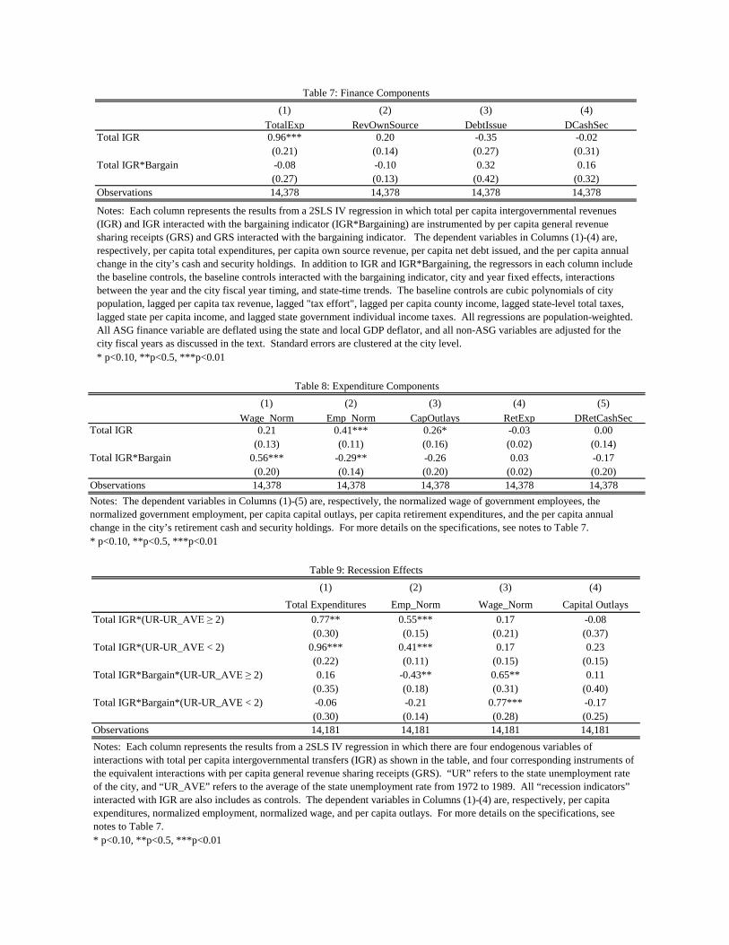
(1) (2) (3) (4)TotalExp RevOwnSource DebtIssue DCashSec

Total IGR 0.96*** 0.20 -0.35 -0.02(0.21) (0.14) (0.27) (0.31)

Total IGR*Bargain -0.08 -0.10 0.32 0.16(0.27) (0.13) (0.42) (0.32)

Observations 14,378 14,378 14,378 14,378

* p<0.10, **p<0.5, ***p<0.01

Table 7: Finance Components

Notes: Each column represents the results from a 2SLS IV regression in which total per capita intergovernmental revenues (IGR) and IGR interacted with the bargaining indicator (IGR*Bargaining) are instrumented by per capita general revenue sharing receipts (GRS) and GRS interacted with the bargaining indicator. The dependent variables in Columns (1)-(4) are, respectively, per capita total expenditures, per capita own source revenue, per capita net debt issued, and the per capita annual change in the city’s cash and security holdings. In addition to IGR and IGR*Bargaining, the regressors in each column include the baseline controls, the baseline controls interacted with the bargaining indicator, city and year fixed effects, interactions between the year and the city fiscal year timing, and state-time trends. The baseline controls are cubic polynomials of city population, lagged per capita tax revenue, lagged "tax effort", lagged per capita county income, lagged state-level total taxes, lagged state per capita income, and lagged state government individual income taxes. All regressions are population-weighted. All ASG finance variable are deflated using the state and local GDP deflator, and all non-ASG variables are adjusted for the city fiscal years as discussed in the text. Standard errors are clustered at the city level.

(1) (2) (3) (4) (5)Wage Norm Emp Norm CapOutlays RetExp DRetCashSec

0.21 0.41*** 0.26* -0.03 0.00(0.13) (0.11) (0.16) (0.02) (0.14)

0.56*** -0.29** -0.26 0.03 -0.17(0.20) (0.14) (0.20) (0.02) (0.20)

Observations 14,378 14,378 14,378 14,378 14,378

* p<0.10, **p<0.5, ***p<0.01

Table 8: Expenditure Components

Notes: The dependent variables in Columns (1)-(5) are, respectively, the normalized wage of government employees, the normalized government employment, per capita capital outlays, per capita retirement expenditures, and the per capita annual change in the city’s retirement cash and security holdings. For more details on the specifications, see notes to Table 7.

Total IGR

Total IGR*Bargain

(1) (2) (3) (4)Total Expenditures Emp_Norm Wage_Norm Capital Outlays

Total IGR*(UR-UR_AVE ≥ 2) 0.77** 0.55*** 0.17 -0.08(0.30) (0.15) (0.21) (0.37)

Total IGR*(UR-UR_AVE < 2) 0.96*** 0.41*** 0.17 0.23(0.22) (0.11) (0.15) (0.15)

Total IGR*Bargain*(UR-UR_AVE ≥ 2) 0.16 -0.43** 0.65** 0.11(0.35) (0.18) (0.31) (0.40)

Total IGR*Bargain*(UR-UR_AVE < 2) -0.06 -0.21 0.77*** -0.17(0.30) (0.14) (0.28) (0.25)

Observations 14,181 14,181 14,181 14,181

* p<0.10, **p<0.5, ***p<0.01

Table 9: Recession Effects

Notes: Each column represents the results from a 2SLS IV regression in which there are four endogenous variables of interactions with total per capita intergovernmental transfers (IGR) as shown in the table, and four corresponding instruments of the equivalent interactions with per capita general revenue sharing receipts (GRS). “UR” refers to the state unemployment rate of the city, and “UR_AVE” refers to the average of the state unemployment rate from 1972 to 1989. All “recession indicators” interacted with IGR are also includes as controls. The dependent variables in Columns (1)-(4) are, respectively, per capita expenditures, normalized employment, normalized wage, and per capita outlays. For more details on the specifications, see notes to Table 7.

(1) (2) (3) (4) (5)

Total IGR 0.96*** 1.03*** 0.92*** 0.87*** 0.81***(0.21) (0.19) (0.21) (0.22) (0.20)

Total IGR*Bargain -0.08 0.02 0.10 0.03 0.04(0.27) (0.27) (0.26) (0.25) (0.20)

Total IGR 0.21 0.37* 0.36** 0.17 0.18(0.13) (0.20) (0.16) (0.10) (0.15)

Total IGR*Bargain 0.56*** 0.40 0.38* 0.14 0.08(0.20) (0.25) (0.23) (0.15) (0.14)

Total IGR 0.41*** 0.47*** 0.33*** 0.42*** 0.16(0.11) (0.18) (0.10) (0.12) (0.17)

Total IGR*Bargain -0.29** -0.37** -0.15 -0.00 0.03(0.14) (0.14) (0.14) (0.18) (0.17)

Population Weighted X X X XPop Cutoff No Top 5Bargain Measure Standard Union Dues Scope: Wages Standard StandardObservations 14,378 14,378 14,360 14,288 14,378

* p<0.10, **p<0.5, ***p<0.01

Table 10: Robustness I

Notes: Each column represents the results from a 2SLS IV regression in which total per capita intergovernmental revenues (IGR) and IGR interacted with the bargaining indicator (IGR*Bargaining) are instrumented by per capita general revenue sharing receipts (GRS) and GRS interacted with the bargaining indicator. The dependent variables in the top, middle, and bottom panels are, respectively, per capita expenditures, normalized wages, and normalized employment. Alternative bargaining measures are used in Columns (2) and (3) as described in the text. In Column (4), the top 5 largest cities are dropped, and in Column (5), the regression is not population-weighted. For more details on the specifications, see notes to Table 7.

Total Expenditures

Normalized Wages

Normalized Employment

(1) (2) (3) (4) (5)

Total IGR 0.96*** 0.96*** 0.90*** 0.98*** 1.02***(0.21) (0.21) (0.29) (0.21) (0.20)

Total IGR*Bargain -0.08 -0.07 -0.07 -0.17 -0.13(0.27) (0.27) (0.27) (0.26) (0.28)

Total IGR 0.21 0.22 0.21 0.22* 0.22(0.13) (0.13) (0.22) (0.13) (0.14)

Total IGR*Bargain 0.56*** 0.55*** 0.55*** 0.56*** 0.56**(0.20) (0.20) (0.21) (0.21) (0.22)

Total IGR 0.41*** 0.41*** 0.31** 0.41*** 0.42***(0.11) (0.11) (0.15) (0.11) (0.11)

Total IGR*Bargain -0.29** -0.29** -0.29** -0.32** -0.27*(0.14) (0.14) (0.13) (0.14) (0.14)

Baseline Controls X X X X XParty of Governor X XParty of Governor*GRS XCity 3-Factor Formula X XState 3-Factor Formula XObservations 14,378 14,378 14,378 14,378 14,378

* p<0.10, **p<0.5, ***p<0.01

Table 11: Robustness II

Total Expenditures

Normalized Wages

Normalized Employment

Notes: Each column represents the results from a 2SLS IV regression in which total per capita intergovernmental revenues (IGR) and IGR interacted with the bargaining indicator (IGR*Bargaining) are instrumented by per capita general revenue sharing receipts (GRS) and GRS interacted with the bargaining indicator. The dependent variables in the top, middle, and bottom panels are, respectively, per capita expenditures, normalized wages, and normalized employment. Column (2) includes as a control an indicator for whether the city was residing in a state with a democratic governor. Data were received from Professor Jim Snyder. Column (2) includes the interaction of this indicator with GRS. Column (4) includes the product of city-level population, tax effort, and inverse per capita income. Column (5) includes, in addition, the product of state-level population, tax effort, and inverse per capita income. For more details on the specifications, see notes to Table 7.

(1) (2) (3) (4) (5)

Emp_Norm BEA Gov't Employees

BEA Private and Gov't Employees

Scaled IGR 0.41*** 10.83*** 14.52*** 9.87* 31.99*(0.11) (2.87) (5.28) (5.53) (17.98)

Scaled IGR*Bargain -0.29** -8.27*** -15.54*** -12.65** -45.04**(0.14) (3.18) (4.66) (5.47) (22.25)

City-County Population Ratio Cutoff 0 0 0.5 0.5 0.5

Observations 14,379 14,379 3,705 3,705 3,705

* p<0.10, **p<0.5, ***p<0.01

Table 12: Macroeconomics Crosswalk

City Gov't Employees (1000)

Notes: Each column represents the results from a 2SLS IV regression in which total per capita intergovernmental revenues (IGR) and IGR interacted with the bargaining indicator (IGR*Bargaining) are instrumented by per capita general revenue sharing receipts (GRS) and GRS interacted with the bargaining indicator. The dependent variables in Columns (1)-(5) are, respectively, per capita normalized city government employment, city government employment per 1000 in the city population, city government employment per 1000 in the city population, total government employment per 1000 in the county population, and total employment per 1000 in the county population. Columns (3)-(5) limit the sample to cities that make up at least 50 percent of their counties. To scale appropriately in Columns (4) and (5), the per capita city intergovernmental transfers are scaled by the county area to city IGR ratio from the most recent government census year. This scaling is discussed and explained in the text. For more details on the specifications, see notes to Table 7.

(1) (2) (3) (4) (5)

Scaled IGR 31.99* 14.84 5.50 52.59* 33.76*(17.98) (15.98) (40.53) (26.85) (18.19)

Scaled IGR*Bargain -45.04* -29.62* -15.79 -50.56** 23.51(22.25) (17.47) (25.12) (19.70) (30.03)

State*Time Trend X X X XUnion Interactions X X X X XPopulation Cutoff No Top 5City-County Population Ratio Cutoff 0.5 0.3 0.85 0.5 0.5

Observations 3,705 6,308 631 3,705 3,515

* p<0.10, **p<0.5, ***p<0.01

Table 13: Macroeconomic Effects

Total Employment (1000 per capita)

Notes: Each column represents the results from a 2SLS IV regression in which total per capita intergovernmental revenues (IGR) and IGR interacted with the bargaining indicator (IGR*Bargaining) are instrumented by per capita general revenue sharing receipts (GRS) and GRS interacted with the bargaining indicator. The dependent variable is total employment per 1000 in the county population. In Columns (1), (4), and (5), the sample is limited to cities that make up at least 50 percent of their counties, in Column (2), the sample is limited to cities that make up at least 30 percent of their counties, and in Column (3), the sample is limited to cities that make up at least 85 percent of their counties. In Column (4), state-time trends are not included, and in Column (5), the top 5 largest cities are dropped. For more details on the specifications, see notes to Table 7.

Figures

0

10

20

30

40

50

60

70

80

90

100

0

2

4

6

8

10

12

14

16

18

Percent of Public Covered by Union

Percent of Private Covered by Union

Public, Covered by Union

Private, Covered by Union

Figure 1: Public and Private Union CoverageMillions of workers Percent

Notes: From Unionstats.com, Hirsch, Macpherson (2011).

Figure 4: State Area Allocations

Notes: Data are from the 1977 Annual Survey of Governments. Amounts are per capita amounts in 2005 dollars.

0

5

10

15

20

25

30

35

40

1971

1972

1973

1974

1975

1976

1977

1978

1979

1980

1981

1982

1983

1984

1985

1986

1987

1988

1989

1990

1991

1992

1993

1994

1995

1996

1997

1998

1999

2000

Figure 3: Federal IGR and General Revenue Sharing FundsBillions of 2005 dollars

Notes: From the 1971-2000 Annual Surveys of Government Finance.

General Revenue Sharing Funds

Total Federal Intergovernmental Transfers

0

20

40

60

80

100

120

140

160

Figure 5: 1977 General Revenue Sharing TransfersNumber of Cities

Notes: Data are from the 1977 Census of Governments, and are de-meaned.

GRS (Per Capita, 2005 dollars)

0

50

100

150

200

250

300

350

Figure 6: 1977 General Revenue Sharing VariationNumber of Cities

Notes: This histogram shows the residuals produced by the regression of per capita general revenue sharing against cubic polynomials of all of the allocation variables as described in the text.

GRS - E[GRS|X] (per capita, real 2005 dollars)

0

5

10

15

20

25

30

Federal DefenseFederal NondefenseStateLocal

Figure 7: Government Consumption and InvestmentPercent of GDP

Notes: Bureau of Economic Analysis NIPA Tables 1.15, 3.20, and 3.21.

-20

0

20

40

60

80

100

120

140

160

1959

1960

1961

1962

1963

1964

1965

1966

1967

1968

1969

1970

1971

1972

1973

1974

1975

1976

1977

1978

1979

1980

1981

1982

1983

1984

1985

1986

1987

1988

1989

1990

Figure 8: Timing of Bargaining Law Passage

MA

Number of cities

AK ID WI

UT

CA

VAWV

OR

CTDE MI MN MD NM

IL

NYRI VT WA AR

NJINME NE NV SD

HIIA PA

KSLA

MTAZ

FL

VASC

OH

Notes: Bargaining legislation data from Freeman and Valletta, 1987. The year marked represents the first full year after which the law was changed.

Figure 9: 1972 Bargaining Laws

Notes: Dark red represents the existence of a pro-union collective bargaining law in 1977. Light red indicates either the absence of such a law, or the existence of a law specifically prohibiting collective bargaining.

0

2

4

6

8

10

12

1948 1953 1958 1963 1968 1973 1978 1983 1988 1993 1998 2003 2008

Figure 10: National Unemployment RatePercent

Source: Bureau of Labor Statistics.

1948 to 2010 average (5.7)

GRS

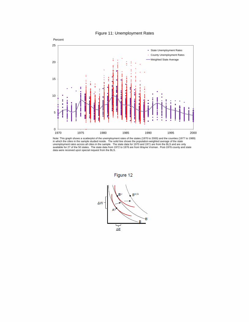
0

5

10

15

20

25

1970 1975 1980 1985 1990 1995 2000

State Unemployment Rates

County Unemployment Rates

Weighted State Average

Figure 11: Unemployment RatesPercent

Note: This graph shows a scatterplot of the unemployment rates of the states (1970 to 2000) and the counties (1977 to 1989) in which the cities in the sample studied reside. The solid line shows the population-weighted average of the state unemployment rates across all cities in the sample. The state data for 1970 and 1971 are from the BLS and are only available for 27 of the 50 states. The state data from 1972 to 1976 are from Wayne Vroman. Post-1976 county and state data were received upon special request from the BLS.