General Relativity Physics Honours 2009

General RelativityPhysics Honours 2009

Florian GirelliRm 364, [email protected]

Lecture Notes 6

http://www.physics.usyd.edu.au/~gfl/Lecture

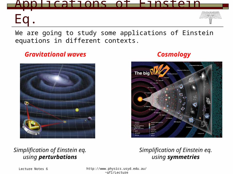
Applications of Einstein Eq.We are going to study some applications of Einstein equations in different contexts.

Lecture Notes 6

CosmologyGravitational waves

Simplification of Einstein eq.using perturbations

Simplification of Einstein eq.using symmetries


Metric perturbations

Chpt 16 & 21 & 23

In physics, we often analyze a system by looking at what happens to perturbations (cf quantum field theory). To simplify the Einstein equations, we can consider a fixed background metric and look at the behavior of perturbations around it

To simplify the analysis, we consider the background metric to be the Minkowski metric: diag(-1,+1,+1,+1)

is the metric perturbation. In effect, we are going to study the dynamics of the symmetric tensor field propagating on Minkowski space: linearized General Relativity.

Lecture Notes 6


Gravitational waves

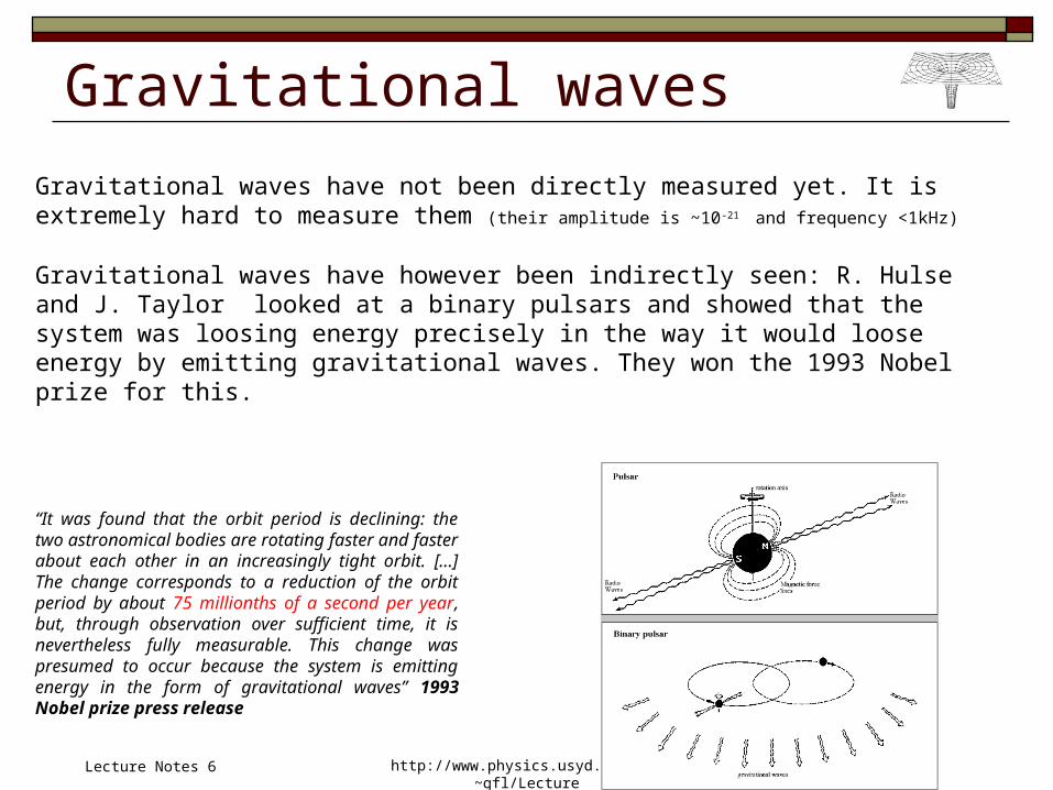
Gravitational waves have not been directly measured yet. It is extremely hard to measure them (their amplitude is ~10-21 and frequency <1kHz)

Gravitational waves have however been indirectly seen: R. Hulse and J. Taylor looked at a binary pulsars and showed that the system was loosing energy precisely in the way it would loose energy by emitting gravitational waves. They won the 1993 Nobel prize for this.

“It was found that the orbit period is declining: the two astronomical bodies are rotating faster and faster about each other in an increasingly tight orbit. […] The change corresponds to a reduction of the orbit period by about 75 millionths of a second per year, but, through observation over sufficient time, it is nevertheless fully measurable. This change was presumed to occur because the system is emitting energy in the form of gravitational waves” 1993 Nobel prize press release

Lecture Notes 6


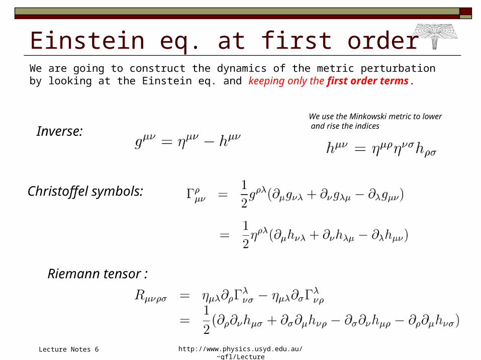
Einstein eq. at first order We are going to construct the dynamics of the metric perturbation by looking at the Einstein eq. and keeping only the first order terms.

Christoffel symbols:

Inverse:We use the Minkowski metric to lower and rise the indices

Riemann tensor :

Lecture Notes 6


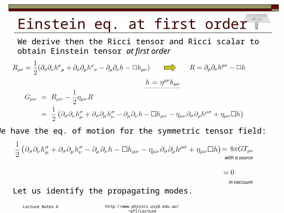
Einstein eq. at first order We derive then the Ricci tensor and Ricci scalar to obtain Einstein tensor at first order

We have the eq. of motion for the symmetric tensor field:

Let us identify the propagating modes.

with a source

in vaccuum

Lecture Notes 6


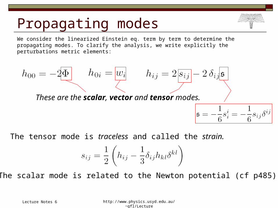
Propagating modesWe consider the linearized Einstein eq. term by term to determine the propagating modes. To clarify the analysis, we write explicitly the perturbations metric elements:

These are the scalar, vector and tensor modes.

The tensor mode is traceless and called the strain.

The scalar mode is related to the Newton potential (cf p485).

Lecture Notes 6


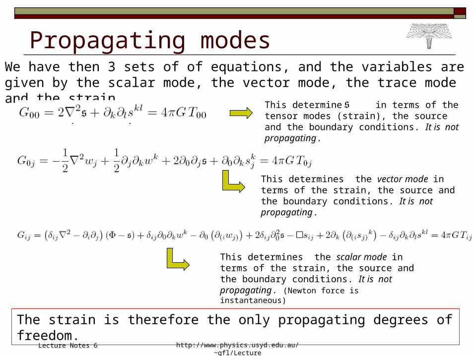
Propagating modes

This determines in terms of the tensor modes (strain), the source and the boundary conditions. It is not propagating.

We have then 3 sets of of equations, and the variables are given by the scalar mode, the vector mode, the trace mode and the strain.

The strain is therefore the only propagating degrees of freedom.

This determines the vector mode in terms of the strain, the source and the boundary conditions. It is not propagating.

This determines the scalar mode in terms of the strain, the source and the boundary conditions. It is not propagating. (Newton force is instantaneous)

Lecture Notes 6


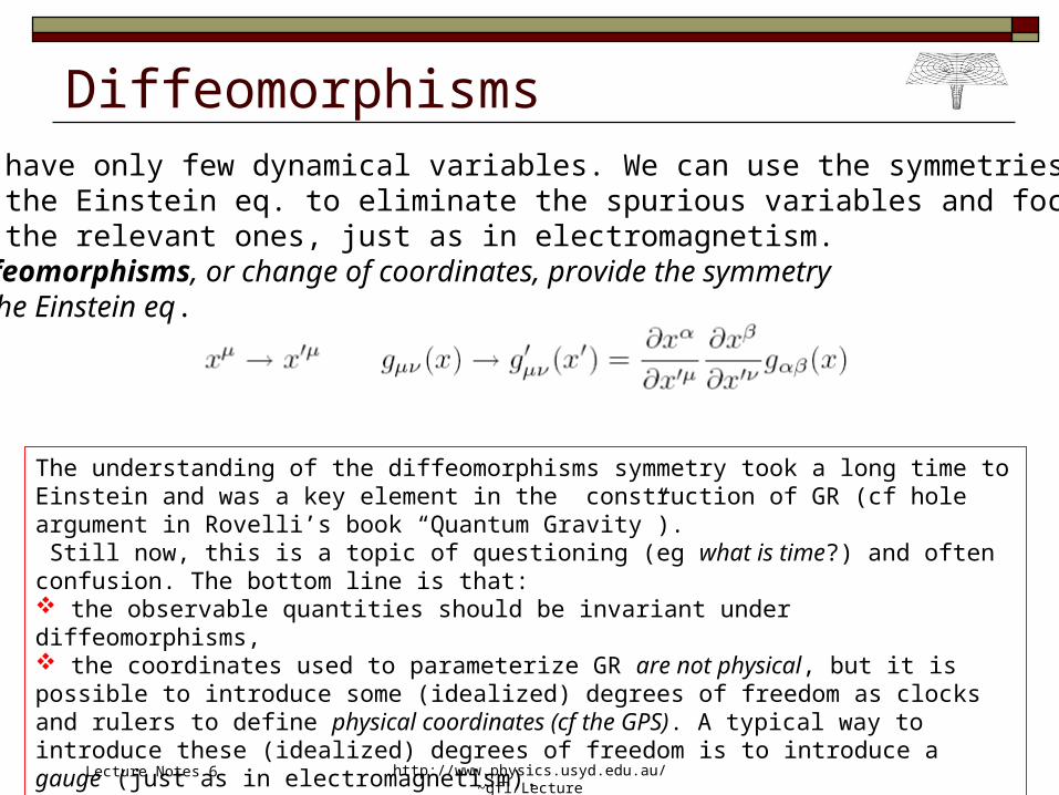
DiffeomorphismsWe have only few dynamical variables. We can use the symmetriesof the Einstein eq. to eliminate the spurious variables and focus on the relevant ones, just as in electromagnetism.Diffeomorphisms, or change of coordinates, provide the symmetryof the Einstein eq.

The understanding of the diffeomorphisms symmetry took a long time to Einstein and was a key element in the construction of GR (cf hole argument in Rovelli’s book “Quantum Gravity”). Still now, this is a topic of questioning (eg what is time?) and often confusion. The bottom line is that: the observable quantities should be invariant under diffeomorphisms, the coordinates used to parameterize GR are not physical, but it is possible to introduce some (idealized) degrees of freedom as clocks and rulers to define physical coordinates (cf the GPS). A typical way to introduce these (idealized) degrees of freedom is to introduce a gauge (just as in electromagnetism).

Lecture Notes 6


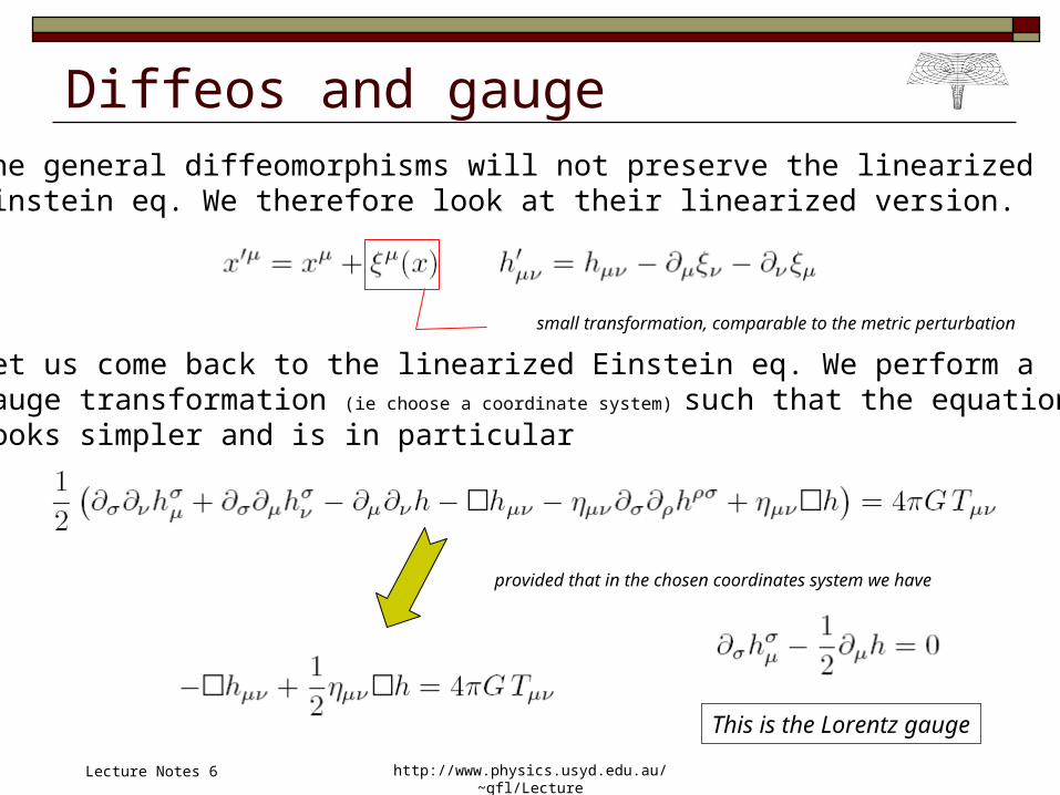
Diffeos and gaugeThe general diffeomorphisms will not preserve the linearized Einstein eq. We therefore look at their linearized version.

small transformation, comparable to the metric perturbation

Let us come back to the linearized Einstein eq. We perform agauge transformation (ie choose a coordinate system) such that the equation looks simpler and is in particular

This is the Lorentz gauge

provided that in the chosen coordinates system we have

Lecture Notes 6


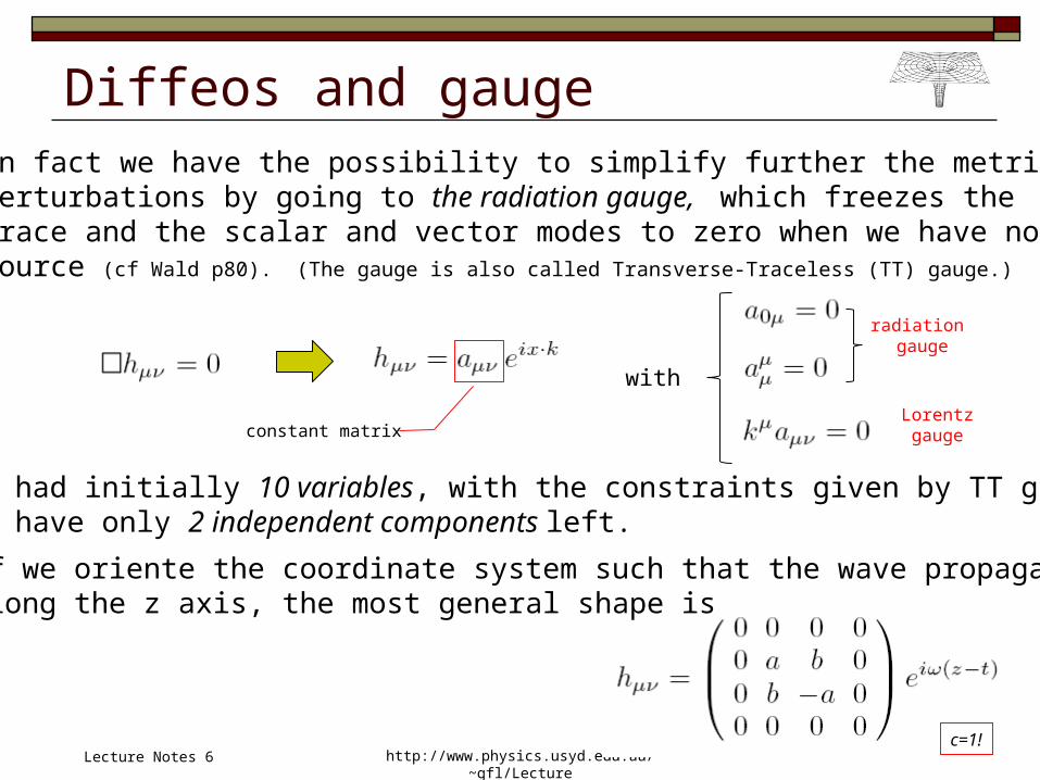
Diffeos and gaugeIn fact we have the possibility to simplify further the metricperturbations by going to the radiation gauge, which freezes the trace and the scalar and vector modes to zero when we have no source (cf Wald p80). (The gauge is also called Transverse-Traceless (TT) gauge.)

with

radiation gauge

Lorentzgauge

We had initially 10 variables, with the constraints given by TT gauge,we have only 2 independent components left.

constant matrix

If we oriente the coordinate system such that the wave propagate along the z axis, the most general shape is

c=1!Lecture Notes 6


Polarization

Key-points: The emitted radiation is not isotropic: it will be stronger in some directions than in others.

Spherically-symmetric motions do not emit any gravitational radiation.

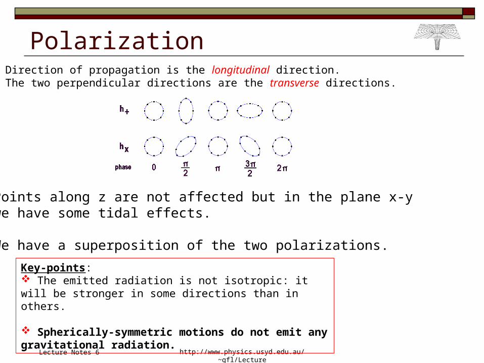
Direction of propagation is the longitudinal direction.The two perpendicular directions are the transverse directions.

Points along z are not affected but in the plane x-ywe have some tidal effects.

We have a superposition of the two polarizations.

Lecture Notes 6


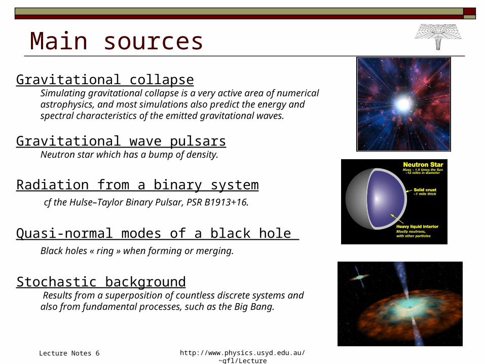
Main sourcesGravitational collapse

Simulating gravitational collapse is a very active area of numerical astrophysics, and most simulations also predict the energy and spectral characteristics of the emitted gravitational waves.

Gravitational wave pulsarsNeutron star which has a bump of density.

Radiation from a binary system cf the Hulse–Taylor Binary Pulsar, PSR B1913+16.

Quasi-normal modes of a black hole Black holes « ring » when forming or merging.

Stochastic background Results from a superposition of countless discrete systems and also from fundamental processes, such as the Big Bang.

Lecture Notes 6


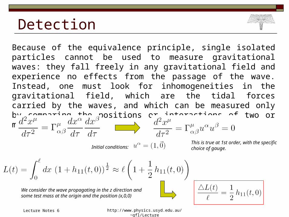
DetectionBecause of the equivalence principle, single isolated particles cannot be used to measure gravitational waves: they fall freely in any gravitational field and experience no effects from the passage of the wave. Instead, one must look for inhomogeneities in the gravitational field, which are the tidal forces carried by the waves, and which can be measured only by comparing the positions or interactions of two or more particles.

Initial conditions:This is true at 1st order, with the specificchoice of gauge.

We consider the wave propagating in the z direction and some test mass at the origin and the position (x,0,0)

Lecture Notes 6


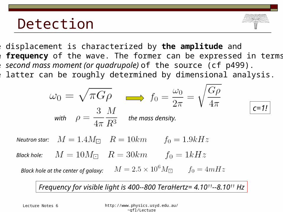
DetectionThe displacement is characterized by the amplitude and the frequency of the wave. The former can be expressed in terms ofthe second mass moment (or quadrupole) of the source (cf p499). The latter can be roughly determined by dimensional analysis.

the mass density.

Neutron star:

Black hole:

Black hole at the center of galaxy:

Frequency for visible light is 400--800 TeraHertz= 4.1011--8.1011 Hz

with

c=1!

Lecture Notes 6


Experiments

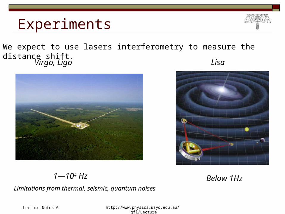
Virgo, Ligo Lisa

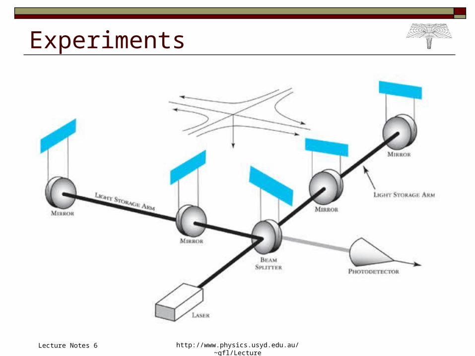
We expect to use lasers interferometry to measure the distance shift.

1—104 Hz

Limitations from thermal, seismic, quantum noises

Below 1Hz

Lecture Notes 6


Experiments

Lecture Notes 6


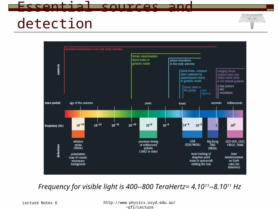
Essential sources and detection

Frequency for visible light is 400--800 TeraHertz= 4.1011--8.1011 Hz

Lecture Notes 6


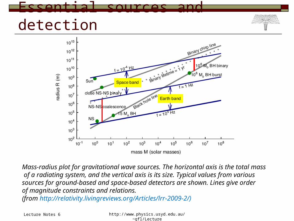
Essential sources and detection

Mass-radius plot for gravitational wave sources. The horizontal axis is the total mass of a radiating system, and the vertical axis is its size. Typical values from various sources for ground-based and space-based detectors are shown. Lines give orderof magnitude constraints and relations. (from http://relativity.livingreviews.org/Articles/lrr-2009-2/)

Lecture Notes 6


« In the linear approximation, General Relativity reduces to the theory of a massless spin 2 field. The full theory of GR thus may be viewed as that of a massless spin 2 field which undergoes some non-linear self-interaction. It should be noted however that the notion of mass and spin require the presence of a flat background metric which one has in the linear theory, but not in the full theory, so that the statement that, in GR, gravity is treated as a massless spin 2 field is not one that can be given meaning outside the context of the linear approximation » Bob Wald, General Relativity, p76

To quantize GR is not the same as simply dealing with gravitons!

Lecture Notes 6

Documents

General Relativity Physics Honours 2009