General Relativity and Dynamical Universes

Bachelor thesis

Author: Kajsa FranssonSupervisor: Daniel Panizo PerezSubject reader: Ulf Danielsson

Uppsala UniversityDepartment of Physics and Astronomy

Division of Theoretical Physics

June 2021

Abstract

The aim of this report is to explore different models of cosmology, depending on components asmatter, radiation and dark energy. To be able to investigate the behaviour and age of these modeluniverses, it is necessary to solve the Friedmann equation. Therefore a substantial part of thisthesis is a study of general relativity, including mathematical tools as Riemannian geometry and theconcept of curved space-time.

Denna rapport amnar att utforska olika kosmologiska modeller beroende pa innehall som materia,stralning och mork energi. For att undersoka beteendet och aldern av dessa modellerade universa saar det nodvandigt att losa Friedmann-ekvationen. Darfor agnas en betydande del av detta arbete atatt studera allman relativitetsteori, med matematiska verktyg som Riemanngeometri och konceptetkrokt rum-tid.

1

Contents

1 Introduction 3

2 Mathematical Tool-kit 42.1 Special Relativity . . . . . . . . . . . . . . . . . . . . . . . . . . . . . . . . . . . . . . 42.2 General Relativity . . . . . . . . . . . . . . . . . . . . . . . . . . . . . . . . . . . . . 7

3 Cosmology 143.1 The Standard Model of Cosmology . . . . . . . . . . . . . . . . . . . . . . . . . . . . 143.2 Content of the Universe . . . . . . . . . . . . . . . . . . . . . . . . . . . . . . . . . . 153.3 Energy of the Universe . . . . . . . . . . . . . . . . . . . . . . . . . . . . . . . . . . . 173.4 ΛCDM-model . . . . . . . . . . . . . . . . . . . . . . . . . . . . . . . . . . . . . . . . 183.5 Big Bang Basics . . . . . . . . . . . . . . . . . . . . . . . . . . . . . . . . . . . . . . 183.6 The Hubble Constant . . . . . . . . . . . . . . . . . . . . . . . . . . . . . . . . . . . 193.7 The Hubble Tension . . . . . . . . . . . . . . . . . . . . . . . . . . . . . . . . . . . . 19

4 Universe and Dynamics 194.1 Empty universe . . . . . . . . . . . . . . . . . . . . . . . . . . . . . . . . . . . . . . . 204.2 Universe With Only Matter . . . . . . . . . . . . . . . . . . . . . . . . . . . . . . . . 214.3 Universe With Only Radiation . . . . . . . . . . . . . . . . . . . . . . . . . . . . . . 234.4 Universe With Only Dark Energy . . . . . . . . . . . . . . . . . . . . . . . . . . . . . 254.5 Universe With Matter and Dark Energy . . . . . . . . . . . . . . . . . . . . . . . . . 274.6 Universe With Radiation And Dark Energy . . . . . . . . . . . . . . . . . . . . . . . 294.7 Universe With Matter And Radiation . . . . . . . . . . . . . . . . . . . . . . . . . . 314.8 ΛCDM -universe . . . . . . . . . . . . . . . . . . . . . . . . . . . . . . . . . . . . . . 33

5 Conclusion 35

Appendix 36

2

1 Introduction

In the middle of the nineteenth century, physicists discovered a peculiar property of the orbit ofMercury around the Sun. Its perihelion (the closest distance to the Sun in the orbit) was not rotatingas slow as Newtonian mechanics predicted. The discrepancy of the measured and calculated valuewas only of 43 arcseconds per century [1]. Still, this problem caused many physicists to tear theirhair trying to propose an explanation that would make the world go back to its Newtonian ways.A number of theories were presented: could it be that undiscovered planets between Mercury andthe Sun affected the orbit? Or maybe some other matter in the plane of the ecliptic? No satisfyingsolution were found.

At roughly the same time James Clark Maxwell proposed the theory of electrodynamics, where thespeed of light was taken to be constant. This was in conflict with the Galilean relativity principle.The inconsistency of the theories sparked a debate of reference systems in the physical world. Manyattempts to prove the existence of a light-medium called ”ether” proved unsuccessful. Finally, AlbertEinstein proposed the theory of special relativity to solve the problem, where Lorentz transformationswere used instead of the Galilean transformations [2]. With his theory he described space and time asfundamentally intertwined quantities. Next, Einstein proposed a generalized form of the equivalenceprinciple, making a connection between space-time and gravity. A consequence of this principle wasthat even light should be affected by gravity in some way, where matter could act as a ”gravitationallens”. Einstein started to explore the idea of curved space, an investigation of many years, usingmathematics that had not before been considered of interest by physicists [1]. The result was thetheory of general relativity, with which he laid the foundation of modern cosmology [3]. We willcover the basic tools of this groundbreaking theory in this thesis. Using his new theory Einsteinattempted to calculate the motion of the perihelion of Mercury and got the very same result whichhad confused physicists for decades. In correspondence with a friend Einstein wrote: ”My wildestdreams have been fulfilled. General covariance. Perihelion motion of Mercury wonderfully exact.”

The theory of general relativity marks the starting point of modern cosmology, and the era ofastonishing cosmological discoveries had just begun. It was Edwin Hubble who first connectedthe velocities and distances of nebulae, planting the seed of the theory of an expanding universe.Einstein, who had altered the famous Einstein equation with the cosmological constant Λ to ensurea static universe had to rethink his worldview. Supposedly, he later called the introduction of thisconstant his ”greatest blunder”. However, the cosmological constant would still be playing a role100 years later, as it is now viewed as non-zero - the effect of dark energy. We will return to theconcept of dark energy in the section Cosmology.

The theory of the Big Bang was independently proposed three times from 1927 to 1965 and wastightly connected to the discovery of the expansion. The basic idea was that if the Universe isexpanding, turning back time would lead it to contract, meaning that the universe was born in aninitial singularity. The Big Bang theory predicted that there should be some kind of remnant fromthis event in terms of radiation. When the cosmic background radiation was discovered in 1965 thetheory had been empirically substantiated for the first time.

The development of cosmology research has since accelerated. The field of cosmology which in thefirst half of the 20:th century had a scientific status that was under debate is now a natural part ofphysics research [1]. The ΛCDM -model is the current established model of the universe, offeringpredictions which agrees with empirical data. It describes a smooth universe, consisting of mostly

3

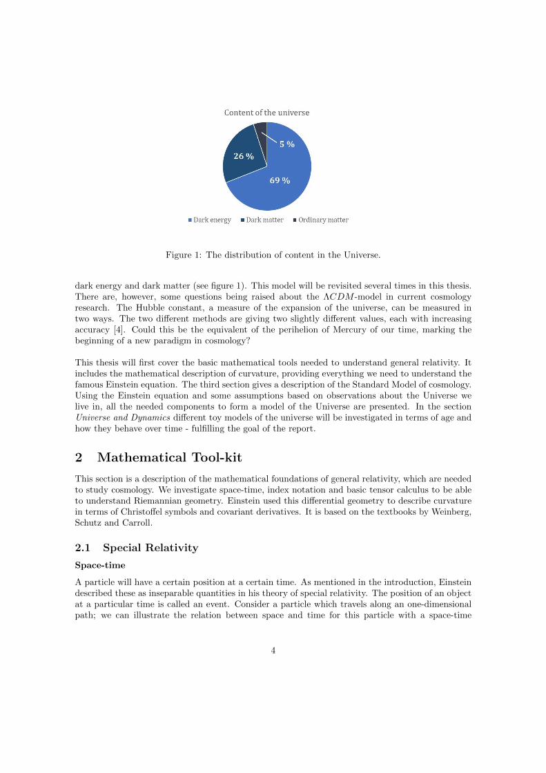
Figure 1: The distribution of content in the Universe.

dark energy and dark matter (see figure 1). This model will be revisited several times in this thesis.There are, however, some questions being raised about the ΛCDM -model in current cosmologyresearch. The Hubble constant, a measure of the expansion of the universe, can be measured intwo ways. The two different methods are giving two slightly different values, each with increasingaccuracy [4]. Could this be the equivalent of the perihelion of Mercury of our time, marking thebeginning of a new paradigm in cosmology?

This thesis will first cover the basic mathematical tools needed to understand general relativity. Itincludes the mathematical description of curvature, providing everything we need to understand thefamous Einstein equation. The third section gives a description of the Standard Model of cosmology.Using the Einstein equation and some assumptions based on observations about the Universe welive in, all the needed components to form a model of the Universe are presented. In the sectionUniverse and Dynamics different toy models of the universe will be investigated in terms of age andhow they behave over time - fulfilling the goal of the report.

2 Mathematical Tool-kit

This section is a description of the mathematical foundations of general relativity, which are neededto study cosmology. We investigate space-time, index notation and basic tensor calculus to be ableto understand Riemannian geometry. Einstein used this differential geometry to describe curvaturein terms of Christoffel symbols and covariant derivatives. It is based on the textbooks by Weinberg,Schutz and Carroll.

2.1 Special Relativity

Space-time

A particle will have a certain position at a certain time. As mentioned in the introduction, Einsteindescribed these as inseparable quantities in his theory of special relativity. The position of an objectat a particular time is called an event. Consider a particle which travels along an one-dimensionalpath; we can illustrate the relation between space and time for this particle with a space-time

4

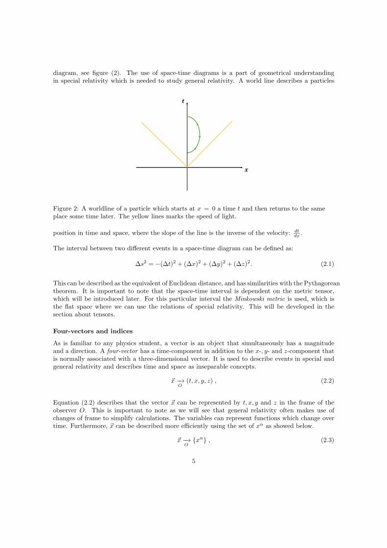
diagram, see figure (2). The use of space-time diagrams is a part of geometrical understandingin special relativity which is needed to study general relativity. A world line describes a particles

Figure 2: A worldline of a particle which starts at x = 0 a time t and then returns to the sameplace some time later. The yellow lines marks the speed of light.

position in time and space, where the slope of the line is the inverse of the velocity: dtdx .

The interval between two different events in a space-time diagram can be defined as:

∆s2 = −(∆t)2 + (∆x)2 + (∆y)2 + (∆z)2. (2.1)

This can be described as the equivalent of Euclidean distance, and has similarities with the Pythagoreantheorem. It is important to note that the space-time interval is dependent on the metric tensor,which will be introduced later. For this particular interval the Minkowski metric is used, which isthe flat space where we can use the relations of special relativity. This will be developed in thesection about tensors.

Four-vectors and indices

As is familiar to any physics student, a vector is an object that simultaneously has a magnitudeand a direction. A four-vector has a time-component in addition to the x-, y- and z-component thatis normally associated with a three-dimensional vector. It is used to describe events in special andgeneral relativity and describes time and space as inseparable concepts.

~x −→O

(t, x, y, z) , (2.2)

Equation (2.2) describes that the vector ~x can be represented by t, x, y and z in the frame of theobserver O. This is important to note as we will see that general relativity often makes use ofchanges of frame to simplify calculations. The variables can represent functions which change overtime. Furthermore, ~x can be described more efficiently using the set of xα as showed below.

~x −→Oxα , (2.3)

5

Where x0 = t, x1 = x, and so on. To describe the same vector according to another observer abar-notation is added for the relevant variables. For equation (2.3) this would mean O → O andα → α. Lorentz transformation is used when switching between different observers (and thereforereference systems), for example: for the time-component we get

x0 =x0

√1− v2

− v · x1

√1− v2

. (2.4)

The velocity v denotes the constant velocity in which one frame moves with respect to the other.Since these transformations produces very long expressions there is notation to describe equation(2.4) in a shorter way. Λ0

β is the coefficient associated with the transformation of the component xβ .

x0 =

3∑β=0

Λ0β x

β . (2.5)

More generally, the sum in the following equation gives the Lorentz transformation for any of thecomponents in ~x,

xα =

3∑β=0

Λαβ xβ . (2.6)

The Einstein summation convention allow us to write equation (2.6) in an even simpler form. Thesummation symbol is neglected, producing notation that makes it easier to give an overview ofcomplicated expressions with many transformations.

xα = Λαβ xβ . (2.7)

Note that it is only due to that both Λ and x has index β that we can use this convention of notation.β is called a dummy index and could be replaced by any other index [5].

Tensors

Vectors previously discussed are called contravariant vectors [2]. These vectors are distinguishedfrom covariant vectors through their individual tangent space and the placement of their indices.Where contravariant vectors have their indices in an ”upstairs” position (see equation 2.7), covariantindices are in ”downstairs” position.

xα = Λβα xβ . (2.8)

Note the opposite order of the indices on the lambda. Both contravariant vectors (referred to as just”vectors”) and covariant vectors (referred to as one-forms) are examples of tensors. The followingdefinition can be given:

”An(MN

)tensor is a linear function of M one-forms and N vectors into the real numbers.” [5]

A(

10

)tensor is a vector, a

(01

)tensor is a one-form. A

(00

)tensor is a called a scalar function which

do not depend on any one-forms or vectors, the kind of function that is introduced in high schoolalgebra.

6

The metric tensorThe metric tensor gµν is an important object - a tensor which describes the geometry of the spacethat is studied. It takes two vectors as arguments and, as it is a tensor, returns a real number. Notethat is has two downstairs indices, which means it is an

(20

)tensor, or a ”two-form”. A contravariant

vector can be transformed to a covariant vector through the metric tensor, and vice versa.

xα = gαβ xβ , xα = gαβ xβ . (2.9)

The space-time interval can be expressed as a function of the metric tensor. In special relativity thespace the metric is called Minkowski space, and to specify this the metric tensor is denoted with ηµν .It is given by ηtt = −1, ηij = 1, i = j 6= t as the only non-zero components, since it is a symmetrictensor. So the space-time interval can be rewritten,

ds2 = −(dt)2 + (dx)2 + (dy)2 + (dz)2 = xµxµ = ηµν x

µxν . (2.10)

The indices µ and ν will both be summed over for every coordinate variable, being dummy indices.Depending on the choice of metric the relation between space and time will vary. As we move intocurved space, the metric will also carry information about the curvature, something we will takeadvantage of later. Different metrics will produce intervals of varying complexity, some very longand annoying. It can be a reassuring thought to keep in mind that we will only handle completelysymmetric metrics in this thesis, simplifying immensely.

Transformation of a tensorThe tensor transformation law is:

Sµ′

ν′ρ′ =∂xµ

′

∂xµ∂xν

∂xν′

∂xρ

∂xρ′Sµνρ. (2.11)

This relation is useful when a change of reference frame is made. It can be done to make calculationseasier, by choosing a reference frame which eliminates certain components of an equation. Also, it isan important notion of the theory of special and general relativity that the equations and relationsthat we find are valid in any coordinate system. We will need this law to understand the covariantderivative later in the thesis [6].

2.2 General Relativity

With the principle of equivalence Albert Einstein connected space-time with gravity. This was thefirst step of the theory of general relativity that would provide answers for many (but not all)problems that had not yet been solved. It involves using differential geometry to describe spaceand then connecting said space to the objects that are located there. In this section selected partsof Riemannian geometry will be presented and the energy-momentum tensor will be explained tofinally arrive at the Einstein equation. With the Einstein equation we are able to construct modelsof the universe, connecting the geometry of a space to the content.

The principle of equivalence

The principle of equivalence can be described in the following way:

7

”At every space-time point in an arbitrary gravitational field it is possible to choose a ’locally in-ertial coordinate system’ such that, within a sufficiently small region of the point in question, thelaws of nature take the same form as in unaccelerated Cartesian coordinate systems in absence ofgravitation.”[2]

So the laws of physics that are true in special relativity still holds in general relativity if the appro-priate frame is chosen, for example the free fall frame. 1 We can relate this to the metric tensor, asit is always possible to make a change of coordinates in which the metric reduces to the Minkowskimetric [2]. One interpretation of the equivalence principle is that gravitation is the cause of thedistortion (curvature) of space-time.

The covariant derivative and Christoffel symbols

As stated earlier, a basic principle in general relativity is that the laws of physics should be validin any coordinate system. Consider the partial derivative, which is present in several equations ofphysics. If we attempt to transform the partial derivative ∂

∂xµ (written in a shorter form as ∂µ) of avector the result below is obtained. The change of frame is made using the transformation law fora tensor, the relation ∂µ′ = ∂xµ

∂xµ′∂µ and the familiar product rule of derivatives.

∂µVµ → ∂µ′V ν

′=( ∂xµ∂xµ′ ∂µ

)(∂xν′

∂xνV ν)

=∂xµ

∂xµ′

∂xν′

∂xν∂µV

ν +∂2xν

′

∂xµ∂xν∂xµ

′

∂xµ′ Vν . (2.12)

For the equation to hold in any frame, the right hand side needs to be tensorial, but the last termis not a tensor. To solve this problem the covariant derivative is introduced, which is invariant(unchanged) during a change of coordinates. The Christoffel symbol Γνµλ is the correction whichcompensates for the non-tensorial part during a transformation. The covariant derivative is givenby the following equation,

∇µV ν = ∂µVν + ΓνµλV

λ. (2.13)

This is a very important definition, since it allows us to generalize obtained results. If a law is truein one frame, it will be true for all frames. If we want to simplify our lives doing calculations, thechoice of a convenient frame is crucial. The definition for the Christoffel symbol is

Γσµν =1

2gρσ(

∂gνρ∂xµ

+∂gµρ∂xν

− ∂gνµ∂xρ

). (2.14)

Depending on the metric the indices will vary between the different coordinate variables. For theMinkowski metric (flat space-time) which has only constant components of the metric, all Christoffelsymbols will be zero. Then the covariant derivative will reduce to just the partial derivative and thelaws of special relativity will hold. When working with plane polar coordinates σ, µ and ν will varybetween r and θ. For example:

Γrθθ =1

2gρr(

∂gθρ∂xθ

+∂gθρ∂xθ

− ∂gθθ∂xρ

). (2.15)

Using the matrix representation of gµν we can get the different values of g. Note that gµν is the

1In a freely falling frame an observer will not measure any acceleration due to gravitation.

8

inverse of gµν .

gµν =

[1 00 r2

](2.16)

Γrθθ =1

2grr(−∂rgθθ) =

1

2· 1 · (−2r) = −r. (2.17)

Curvature

Until the introduction of the concept of curvature, vectors at different points in space were comparedto each other without any consideration of where they were positioned. It turns out that this is onlyvalid due to that in flat space all points are part of the same tangent space. In Euclidean space theshortest distance between two points is the straight line. Consider instead the space which consistsof (the surface of) a sphere with a given radius, which is a curved space. In this space it is notpossible to connect two points with a straight line. The shortest distance will be the line alongwhich the tangent vector can be parallel transported. This distance received the name geodesic.

To understand this better - imagine you are walking on the earth and in your hand you are holdinga stick parallel to the ground. If you are walking the shortest distance from point A to point B youcannot choose the straight line between the points - it would go through the earth. You have to walkalong the surface of the earth, which is curved. For the entirety of your walk you are holding thestick parallel to the ground. When you arrive at point B the stick will have a new direction in space(but is still parallel to the ground). This is the concept of parallel transport, tiny changes to a vectoralong a geodesic which still is tangent to the space at every point. In flat space the derivative givesa value of a rate of change with respect to a certain variable. The covariant derivative is similarly avalue for the rate of change, but now in comparison with a paralleled transported vector.

The Riemann curvature tensorThe covariant derivative of a tensor gives a measure of how much the tensor changes when it istransported in a certain direction, compared to a parallel transported vector. Let us consider thecommutator of two covariant derivatives,

[∇µ,∇ν ]V ρ = ∇µ∇νV ρ −∇ν∇µV ρ. (2.18)

The commutator returns the difference of first taking the covariant derivative in one direction andthen the other, and then doing the same but in opposite order. If this value is zero, and there is nodifference due to choice of direction (for all directions), the space should be flat. We evaluate thefirst term,

∇µ∇νV ρ = ∇µ(∂νVρ + ΓρνσV

σ), (2.19)

∇µ∇νV ρ = ∂µ(∂νVρ + ΓρνσV

σ)− Γλµν(∂λVρ + ΓρλσV

σ) + Γρµλ(∂νVλ + ΓλνσV

σ), (2.20)

∇µ∇νV ρ = ∂µ∂νVρ+∂µΓρνσV

σ+Γρνσ∂µVσ−Γλµν∂λV

ρ−ΓλµνΓρλσVσ+Γρµλ∂νV

λ+ΓρµλΓλνσVσ. (2.21)

Now take into account that in equation 2.18 the second term is just the first term but with µexchanged for ν and vice versa. Evaluate the second term.

−∇ν∇µV ρ = −(∂ν∂µVρ + ∂νΓρµσV

σ + Γρµσ∂νVσ − Γλνµ∂λV

ρ − ΓλνµΓρλσVσ + Γρνλ∂µV

λ + ΓρνλΓλµσVσ).

(2.22)

9

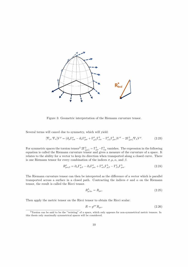
Figure 3: Geometric interpretation of the Riemann curvature tensor.

Several terms will cancel due to symmetry, which will yield:

[∇µ,∇ν ]V ρ = (∂µΓρνσ − ∂νΓρµσ + ΓρµλΓλνσ − ΓρνλΓλµσ)V σ − 2Γλ[µν]∇λVρ. (2.23)

For symmetric spaces the torsion tensor2 2Γλ[µν] = Γλµν−Γλνµ vanishes. The expression in the followingequation is called the Riemann curvature tensor and gives a measure of the curvature of a space. Itrelates to the ability for a vector to keep its direction when transported along a closed curve. Thereis one Riemann tensor for every combination of the indices σ, µ, α, and β.

Rσµαβ = ∂αΓσµβ − ∂βΓσµα + ΓσαλΓλµβ − ΓσβλΓλµα. (2.24)

The Riemann curvature tensor can then be interpreted as the difference of a vector which is paralleltransported across a surface in a closed path. Contracting the indices σ and α on the Riemanntensor, the result is called the Ricci tensor.

Rλµλν = Rµν . (2.25)

Then apply the metric tensor on the Ricci tensor to obtain the Ricci scalar:

R = gµνRµν . (2.26)

2Torsion can be said to be the ”twisting” of a space, which only appears for non-symmetrical metric tensors. Inthis thesis only maximally symmetrical spaces will be considered.

10

The Ricci scalar gives a value of the curvature of a space. While the Riemann tensor and Riccitensor have different results for different combinations of indices, the Ricci scalar is just one scalarvalue. Because of the many symmetries of the Riemann curvature tensor only a fraction of themhave to be calculated. For example: when working with a maximally symmetric metric tensor infour dimensions only 20 tensor components out of 256 have to be calculated [6]. The symmetriesare:

Rσµαβ = Rαβσµ, Rσµαβ = −Rµσαβ , Rσµαβ = −Rσµβα. (2.27)

The amount of components that have to be calculated is depending on the number of dimensions n.

The formula n2(n2−1)12 can be used to determine precisely how many [2].

The energy-momentum tensor

Until now we have only discussed space-time as an empty space. But to get a satisfying model ofthe universe we need to take matter and therefore its energy and momentum into account. To dothis we introduce the energy-momentum tensor Tµν . For a perfect fluid, which we will later see is avery useful approximation of the content of our own Universe, it can be defined as

Tµν = (ρ+ p)UµUν + pgµν . (2.28)

Where both Uµ and Uν is the four-velocity of the particles, the vector from equation 2.2 derivedwith respect to time. The quantity ”energy density” ρ is defined as ρ = nm, where n is the amountof particles per unit volume and m is the mass of a particle. Despite the name of the tensor p standsfor pressure and not momentum. Both p and ρ are defined in rest frame. A perfect fluid is a mediumwhich can be accurately described by these two quantities only. In the rest frame the four-velocitybecomes proportional to (1, 0, 0, 0), and we know from the equivalence principle that we can alwaysfind such a frame (although it might be difficult). At rest the energy-momentum tensor can bedescribed in matrix form as:

(p+ ρ) + pg00 0 0 00 pg11 0 00 0 pg22 00 0 0 pg33

. (2.29)

From Newtonian mechanics and thermodynamics we know that energy and momentum is conservedin flat space-time. The fact that energy cannot be created or destroyed is a relation that has manyimplications in physics, rigorously supported by observations and experiments. Now, using theenergy-momentum tensor we express these important relations as

∂µTµν = 0. (2.30)

For a symmetric energy-momentum tensor the first diagonal component is associated with the con-servation of energy. The remaining diagonal components satisfies the conservation of momentum.As we learned in the previous sections, the partial derivative is flawed as a measure for rate of changein curved space. But we still would like conservation of energy to hold, regardless of the shape ofthe space. To generalize this relationship to general relativity, the covariant derivative is required;

∇µTµν = 0. (2.31)

11

Note that this describes local conservation of energy. According to the equivalence principle it ispossible to find a frame at every point in space-time where energy is conserved. But the same cannotbe stated for global frames [6].

Einstein equation

Now that both Riemannian geometry and the energy-momentum tensor have been covered, we areready to take on the Einstein equation. Albert Einstein’s work on the equivalence principle gavehim the idea that the matter content of the universe could be the cause of space-time curvature. Hewanted to find a relation between the energy-momentum tensor (which describes the properties ofmatter) and the Riemann curvature tensor. Since the covariant derivative of the energy-momentumtensor is zero, the same had to be true for the tensor that describes curvature. Unfortunately, thecovariant derivative of the Riemann curvature tensor is not zero. Einstein then turned to the Bianchiidentity (important in Riemannian geometry and soon to be described), which is zero when actedon by the covariant derivative [5].

The Einstein tensorThe Bianchi identity is given by

∇ [λRµν]αβ = 0, (2.32)

Which can be written∇λRαβµν +∇νRαβλµ +∇µRαβνλ = 0. (2.33)

It is not very difficult to show this if we choose a locally inertial frame. Then all Christoffel symbolswill vanish and the Riemann tensor becomes

Rαβµν = gασRσβµν = gασ(∂µΓσβν − ∂νΓσβµ). (2.34)

Using the definition for the Christoffel symbol Rαβµν is equal to

Rαβµν =1

2(∂µ∂βgνα − ∂µ∂αgνβ − ∂ν∂βgµα + ∂ν∂αgµβ). (2.35)

In exactly the same way we can get an expression for Rαβλµ and Rαβνλ. Since we still are workingwith a locally inertial frame and the Christoffel symbols vanish, the only part of the covariantderivative that remains is the partial derivative. We can rewrite equation (2.33) to

∂λRαβµν + ∂νRαβλµ + ∂µRαβνλ = 0. (2.36)

Substituting the Riemann tensors we get a very long expression, but by careful comparison of thedifferent terms we discover that all will cancel.

1

2(∂λ∂µ∂βgνα − ∂λ∂µ∂αgνβ − ∂λ∂ν∂βgµα + ∂λ∂ν∂αgµβ +

+ ∂ν∂λ∂βgµα − ∂ν∂λ∂αgµβ − ∂ν∂µ∂βgλα + ∂ν∂µ∂αgλβ +

+ ∂µ∂ν∂βgλα − ∂µ∂ν∂αgλβ − ∂µ∂λ∂βgνα + ∂µ∂λ∂αgνβ) = 0.

(2.37)

12

So the left hand side is zero for a locally inertial frame, but since it is a tensor equation we knowthat the result can be generalized for any frame. So now we are confident that the Bianchi identityis true. [2] It is possible to apply the metric tensor on equation (2.33) to make a contraction:

gαµ(∇λRαβµν −∇νRαβµλ +∇µRαβνλ) = 0. (2.38)

Note the change of sign and position of indices of the second term. The covariant derivative of themetric tensor is zero and the metric tensor can therefore be applied directly on the Riemann tensors.It is zero because we know that the covariant derivative of the metric tensor in an inertial frame iszero. That relation is a tensor equation which can be generalized to any frame.

∇λRβν −∇νRβλ +∇µRµβνλ = 0. (2.39)

We make a new contraction and make use of symmetry relations.

gβν(∇λRβν −∇νRβλ −∇µRµβλν) = 0 (2.40)

∇λR−∇νRνλ −∇µRµλ = 0, (2.41)

∇λR−∇µRµλ −∇µRµλ = 0, (2.42)

∇λR− 2∇µRµλ = 0, (2.43)

∇µ(Rµλ −1

2gλµR) = 0, (2.44)

The result is a tensor depending only on the Riemann curvature tensor and the metric which hasa covariant divergence that is zero. This has the properties sought by Einstein and is the left handside of the famous Einstein equation [5],

Rµν −1

2Rgµν = 8πGTµν . (2.45)

The factor 8πG on the right hand side comes from asserting that this equation should reduce toPoisson’s equation of gravity (stated below) in the Newtonian limit. It also contributes with gettingequal dimensions on each side of the equation. The Newtonian limit means that we assume a weakand static gravitational field and slow movement with respect to speed of light [6].

∇2Φ = 4πGρ. (2.46)

Now that we have acquired all the tools that we need to describe the Einstein equation, it is timeturn to cosmology. Making some standard assumptions of the properties of the Universe, Einsteinequations can be solved.

13

3 Cosmology

This section provides a brief introduction to cosmology, with necessary concepts to be able toinvestigate the different models of the universe in the next section. Many concepts are based onthe cosmological principle, which says that independently of where we look in the universe, we willobserve more or less the same things. The matter content will be approximately the same and thesize of the universe will not be measured differently based on position in the universe [7]. Morespecifically it is said to be both isotropic and homogeneous. Homogenous - we will see the samepattern everywhere and can therefore describe the space with one single metric. Isotropic - thisis true independent on in what direction we look. The cosmic background radiation supports thisdescription, as it is so uniformly distributed [6].

3.1 The Standard Model of Cosmology

The FLRW Metric

We consider the line element

ds2 = −dt2 + a2(t)(dr2

1− kr2+ r2dθ2 + r2sin2θdφ2). (3.1)

The spatial components depend on the scale factor a(t) which is related to the size of the universe.The constant k is associated to the curvature of the universe The associated metric tensor to thisline invariant is called the Friedmann-Lemaıtre-Robertson-Walker (FLRW) metric. This metric isvalid for spaces like the universe we want to study - spaces that are isotropic and homogeneous[7]. The curvature k can be 1, 0 or -1. It is a normalized constant which decides the geometryof the space. This normalization has implications for the solutions describing the behaviour of theuniverse, so it is important to keep in mind in the next section. If the curvature is negative it iscalled an open universe. The closed universe has a positive curvature and a finite size. In that casea(t) is considered to be the radius of the universe (but recall that the universe is not considered tohave a center). For zero curvature the metric reduces to the Minkowski metric, but rescaled withsaid scale factor and is called flat.If we aim to solve the Einstein equation for this metric we must make a choice of an appropriateenergy-momentum tensor.

The Friedmann Equation

For the Standard Model of cosmology the energy-momentum tensor for the perfect fluid is sufficient.Support for this claim can be found in the cosmological principle [7]. In the appendix of this thesisthe Riemann tensor components are calculated for a general metric depending on a time-dependentfunction f(t) and radially dependent function g(r). Substituting for f(t) = a(t)2 and g(r) = 1

1−kr2

the resulting expressions simplifies. The 00 component of the Einstein equation (2.45) will become

R00 −1

2Rg00 = 8πGT00. (3.2)

And for our chosen metric we have:

R00 = −3a

a, g00 = −1, R =

6(aa+ a2 + k)

a2, T00 = ρ. (3.3)

14

We can see that the left hand side, describing the geometry of space-time, is depending on therate of change of the scale factor. After substituting and simplifying we obtain the first Friedmannequation,

a2 + k

a2=

8

3πGρ. (3.4)

Solving for the spatial components will all yield the same equation,

2aa+ a2 + k

a2= −8πGp. (3.5)

But this is linearly dependent on the first Friedmann equation [4]. The difference between the twoequations is

a

a=−4πG(ρ+ 3p)

3. (3.6)

This is called the second Friedmann equation, or sometimes the acceleration equation [7].

3.2 Content of the Universe

There are three different components of the universe that this thesis will investigate. Non relativisticmatter, which will be referred to as just matter. It is referring to both ordinary matter (essentiallyeverything built from atoms) and dark matter. As we will take advantage of later, observations tellsus that the universe is mostly consisting of dark matter and dark energy. Dark matter is not yet verywell described, but is considered to be cold and therefore not relativistic. The second componentis radiation which primarily has an impact on the universe in its early development. Lastly, darkenergy will be taken into account. Dark energy is the component of the universe that is consideredto be the cause of the acceleration of the expansion of the universe. It is the medium that serves asan explanation for the presumed non-zero cosmological constant Λ in the Friedmann equation [6].It was Einstein who introduced the cosmological constant in the Friedmann equation which became

a2

a2+

k

a2=

8πGρ

3+

Λ

3. (3.7)

He introduced it because he believed that the universe was static, and without the cosmologicalconstant the universe was either collapsing or expanding. Matter content contributes to a collapsingfate of the universe. The sign of the constant can be positive or negative, therefore it is valuableto consider negative or positive dark energy. Positive dark energy is expected to make the universeexpand whereas negative dark energy should make the universe collapse even faster. To relate this tothe equation of state described below, positive dark energy is considered to have negative pressure.Since dark energy is theorized as some kind of content in the universe, it is associated with an energydensity3 ρΛ in the same way as radiation and matter [4].

3The energy density for dark energy is taken to be ρΛ = Λ8πG

to be able to consider the cosmological constantas a part of the total energy density in the Friedmann equation.

15

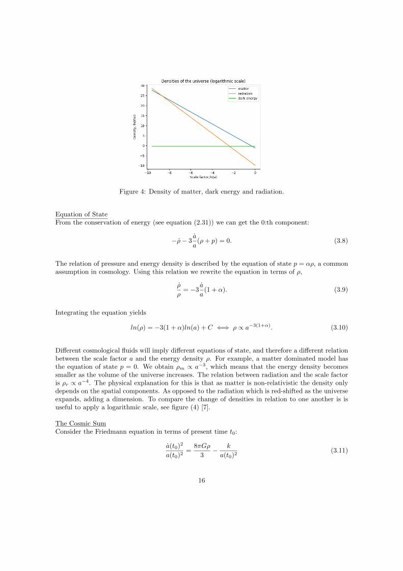
Figure 4: Density of matter, dark energy and radiation.

Equation of StateFrom the conservation of energy (see equation (2.31)) we can get the 0:th component:

−ρ− 3a

a(ρ+ p) = 0. (3.8)

The relation of pressure and energy density is described by the equation of state p = αρ, a commonassumption in cosmology. Using this relation we rewrite the equation in terms of ρ,

ρ

ρ= −3

a

a(1 + α). (3.9)

Integrating the equation yields

ln(ρ) = −3(1 + α)ln(a) + C ⇐⇒ ρ ∝ a−3(1+α). (3.10)

Different cosmological fluids will imply different equations of state, and therefore a different relationbetween the scale factor a and the energy density ρ. For example, a matter dominated model hasthe equation of state p = 0. We obtain ρm ∝ a−3, which means that the energy density becomessmaller as the volume of the universe increases. The relation between radiation and the scale factoris ρr ∝ a−4. The physical explanation for this is that as matter is non-relativistic the density onlydepends on the spatial components. As opposed to the radiation which is red-shifted as the universeexpands, adding a dimension. To compare the change of densities in relation to one another is isuseful to apply a logarithmic scale, see figure (4) [7].

The Cosmic SumConsider the Friedmann equation in terms of present time t0:

a(t0)2

a(t0)2=

8πGρ

3− k

a(t0)2(3.11)

16

The Hubble constant is H0 = a(t0)a(t0) , and a(t0) = a0 so the equation can be rewritten:

1 =8πG

3H20

ρ− k

a20H

20

. (3.12)

Using the definition for critical density ρc =3H2

0

8πG and assuming that the total density consists ofmatter, radiation and dark energy the equation becomes:

1 =ρm + ρr + ρΛ

ρc− k

a0H20

. (3.13)

Using the relation for the density parameter Ωi =ρ0i

ρcand asserting that Ωk = − k

a20H

20

the equation

can be written in terms of density parameters:

1 = Ωm + Ωr + ΩΛ + Ωk. (3.14)

This is called the cosmic sum, and will be of use when we want to look at different contents of theuniverse later.

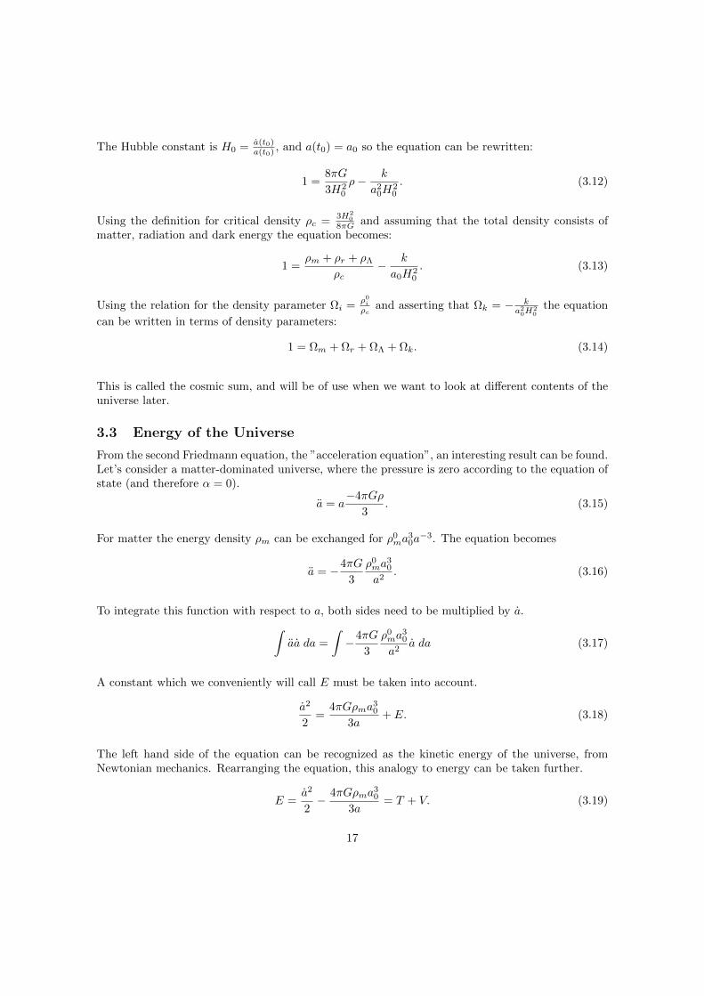
3.3 Energy of the Universe

From the second Friedmann equation, the ”acceleration equation”, an interesting result can be found.Let’s consider a matter-dominated universe, where the pressure is zero according to the equation ofstate (and therefore α = 0).

a = a−4πGρ

3. (3.15)

For matter the energy density ρm can be exchanged for ρ0ma

30a−3. The equation becomes

a = −4πG

3

ρ0ma

30

a2. (3.16)

To integrate this function with respect to a, both sides need to be multiplied by a.∫aa da =

∫−4πG

3

ρ0ma

30

a2a da (3.17)

A constant which we conveniently will call E must be taken into account.

a2

2=

4πGρma30

3a+ E. (3.18)

The left hand side of the equation can be recognized as the kinetic energy of the universe, fromNewtonian mechanics. Rearranging the equation, this analogy to energy can be taken further.

E =a2

2− 4πGρma

30

3a= T + V. (3.19)

17

This is an expression for the total energy for the universe, where the second term is the potentialenergy. It is constructed in a way that is similar to the energy of a rocket launch. If the energyis negative, the kinetic energy cannot overcome the potential energy and the rocket will fall backdown to earth. If the energy is positive the rocket can escape the atmosphere. In a similar way, theuniverse can collapse or expand forever [8].

3.4 ΛCDM-model

Before we can start exploring different models of potential universes, another cosmological topic hasto be introduced - the ΛCDM-model. This model is the most accepted model of the Universe inmodern cosmology due its ability to correctly predict properties of the Universe. It is based on severalassumptions, some of them we have already covered - as the evolution of the density distributionof the universe. The ΛCDM-model describes a universe that first is dominated by radiation, tothen be dominated by matter and lastly by dark energy. According to the model, the Universe istoday consisting of mostly dark energy (Λ) and cold dark matter (CDM). The notion of dark matterhad to be introduced by astronomers to explain the behaviour of certain galaxies, whose movementcould not be the consequence of just ordinary matter. As mentioned before, the dark energy Λ wasoriginally just a constant which Einstein introduced in order to get a static universe [9]. But theuniverse was not only discovered to be expanding, but seems to be expanding faster and faster [10].In current cosmology the cosmological constant is therefore considered to be non-zero, since it isneeded to account for the accelerated expansion that the Universe seems to be going through.Another important property of the universe according to the ΛCDM-model is the overall smoothnessof the universe. The cosmic microwave background radiation supports the notion that the earlyuniverse was homogeneous. In modern cosmology the curvature of the universe is often assumed tobe flat, sometimes called an Euclidian Universe. This is also substantiated through measurementsof the properties of the CMB [9].

3.5 Big Bang Basics

As mentioned earlier, the Standard Model of cosmology includes the theory of Big Bang, whichdescribes the birth of the accelerated expanding universe. The theory is in principle built on thatsince we live in an expanding universe, going backwards in time must mean that all matter issqueezed together - in a gravitational singularity. Thus the universe must have been born in a stateof very high temperature and density. [4] We have already stated that the Universe was dominatedby radiation in its early state. A natural conclusion to this information is that there should besome kind of trace of this radiation. But at the high temperature of the early Universe that the BigBang theory suggests, it is abundant with free electrons. The electrons and photons are interacting,making the photons bounce back and forth hindering transmission over long distances. This is whywe can’t see any trace of the radiation from the really early universe. The earliest traces of radiation(and therefore the Big Bang) is instead seen in the cosmic microwave background radiation (CMB).It is the consequence of recombination, when the free electrons had lost so much energy that theyrather would be combined with a proton. The amount of particles that the photons could interactwith decreased and the universe became ”transparent”, allowing us to observe the CMB [6].

18

3.6 The Hubble Constant

Edwin Hubble discovered that depending on the distance to a galaxy, it will move away from uswith a certain velocity. It turns out that the greater the distance, the greater the velocity of thegalaxy. This was the first observation that suggested that the universe was expanding, not staticas Einstein thought [7]. The Hubble constant is defined as the ratio between the velocity and thedistance to an object in space, H0 = v

d . The velocity is measured through the redshift, and thedistance is measured by a method that depends on standard candles [4]. Although the cosmologicalprinciple states that the universe is isotropic, objects in space are moving in relation to each other.This is called peculiar motion, and when looking at a specific object the cosmological principle willnot hold, so it must be taken into account. We want to be able to distinguish the velocity due to theacceleration of the universe and the peculiar motion. This means that we want to observe objectsfar away, as their velocity due to expansion is then much bigger than the peculiar motion. This doesnot make us happy, as it is much harder to measure distances far away. The geometrical method ofparallax which gives reliable values of distances cannot be used when looking sufficiently far away.Instead, the method is built on standard candles. The method is to compare the brightness of anobject that we want to know the distance of to an object of the same type that is closer and thereforehave a measurable distance.

3.7 The Hubble Tension

There is another way to measure the Hubble constant, taking advantage of the radiation remainingfrom the Big Bang. To get a value from the measurements from the CMB, the ΛCDM -modelhas to be utilized [4]. Depending on what assumptions are made about the universe (e.g. itscurvature and content) the model will predict different characteristics of the CMB. Of course thevalue of the Hubble constant will also affect these predictions. The predictions can be compared tomeasurements of the real CMB. The Planck Collaboration found a value of 67.4 ± 0.5 km/s/Mpcin 2018 based on measurements from the CMB and assumptions made from the ΛCDM -model [11].Comparing this with a typical value from a measurement using the method of standard candles,as H0 = 73.2 ± 1.3 km/s/Mpc raises some eyebrows [12]. The difference between the values isstatistically significant and is called the Hubble tension.

Solutions proposed to ease the tension between the two values are many. A different energy densitydistribution in the early universe with more dark energy is suggested. Another explanation is that theequation of state for dark energy is time-dependent, a ”dynamical dark energy”. Other interestingideas can be categorized as ”unified cosmologies”, describing dark energy and dark matter as twoparts of the same cosmological fluid. Since both matter and dark matter can be observed it is mostappealing to change the description of dark energy in the model. Although there are many differentideas, no consensus has been reached [13].

4 Universe and Dynamics

Finally we have all the tools and background knowledge we need to investigate the fate of theuniverse depending on what it consists of. The different contents are matter, dark energy andradiation. These components are expected to have a dynamical relation, where matter causes theuniverse to collapse and positive dark energy counteract this process. In this section the Friedmannequation will be solved, depending on what the cosmological fluid contains.

19

The first Friedmann equation (3.4) can be rewritten:

a2

a2=

8πGρ

3− k

a2. (4.1)

To discuss the potential energy, recall that the total energy is constant, ∆E = 0. Rewrite the firstFriedmann equation again.

a2 =8πGρa2

3− k. (4.2)

The term that will represent the total energy in the Friedmann equation will be the curvature term,which also is constant. The kinetic energy will be the term containing a2. This means that theremaining term can be taken to be the potential energy.

The age of the universe can be calculated in different ways. If the solution of the Friedmann equationgives a scale factor in terms of time t, we can set the scale factor to its current normalized valuea0 = 1 and solve for t0. If the solution is in conformal time τ , the relation below can be used [8]. Theconformal time is the time as measured in frame moving along with the expansion of the universe(called comoving frame) and is defined by dτ = dt

a(t) [7].

t =

∫dt =

∫a(τ)dτ. (4.3)

Solving for τ and substituting the expression in a(τ) gives a(t). When solving for the time fora certain universe the cosmic sum

∑Ωi = 1 is used to get appropriate values for the density

parameters.

4.1 Empty universe

For an empty universe, the density is taken to be zero and the first Friedmann equation can bewritten

a2

a2= − k

a2. (4.4)

Simplifying, the result is (dadt

)2

= −k. (4.5)

This equation only holds for k = 0 or k = −1, since dadt should not be complex. We can rewrite

k as a function of density parameter for curvature, −k = ΩkH20 . After taking the square root the

equation becomes:da

dt=√

Ωk H0 (4.6)

Possible scale factors are:

a(t) =√

Ωk H0 t, k < 0, (4.7a)

a(t) = const, k = 0. (4.7b)

20

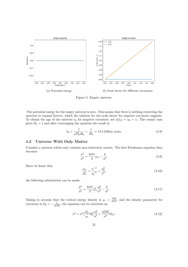
(a) Potential energy. (b) Scale factor for different curvatures.

Figure 5: Empty universe.

The potential energy for the empty universe is zero. This means that there is nothing restricting theuniverse to expand forever, which the solution for the scale factor for negative curvature suggests.To obtain the age of the universe t0 for negative curvature, set a(t0) = a0 = 1. The cosmic sumgives Ωk = 1 and after rearranging the equation the result is:

t0 =1√

ΩkH0

=1

H0= 14.5 billion years. (4.8)

4.2 Universe With Only Matter

Consider a universe which only contains non-relativistic matter. The first Friedmann equation thenbecomes

a2

a2=

8πG

3ρm −

k

a2. (4.9)

Since we know thatρmρ0m

=a−3

a−30

=a3

0

a3, (4.10)

the following substitution can be made:

a2

a2=

8πG

3ρ0m

a30

a3− k

a2. (4.11)

Taking to account that the critical energy density is ρc =3H2

0

8πG , and the density parameter for

curvature is Ωk = − ka2

0H20

, the equation can be rewritten as:

a2 = a2(ρ0M

ρcH2

0

a30

a3+a2

0H20

a2Ωk). (4.12)

21

The density parameter for matter is Ωm =ρ0m

ρcand the current scale factor is a0 = 1. [4]

a2 = H20 (Ωm

1

a+ Ωk). (4.13)

To make it easier to solve for a we make a substitution to conformal time τ . The relation isdadt = da

dτ1

a(τ) . The result is a separable differential equation of the form:

da

dτ= H0

√Ωma+ Ωka2. (4.14)

Since Ωk has a different sign depending on the curvature, there will be several different solutions.These solutions for the scale factor a(τ) becomes

a(τ) =ΩmΩk

sinh2(

√ΩkH0τ

2), k < 0, (4.15a)

a(τ) =Ωm| Ωk |

sin2(

√| Ωk |H0τ

2), k > 0, (4.15b)

a(τ) =H2

0 Ωmτ2

4, k = 0. (4.15c)

Equation (4.13) can be rewritten as

H20 Ωk = a2 −H2

0 Ωm1

a. (4.16)

This means that the potential of this universe can be expressed as

V (a) = −H20 Ωma

. (4.17)

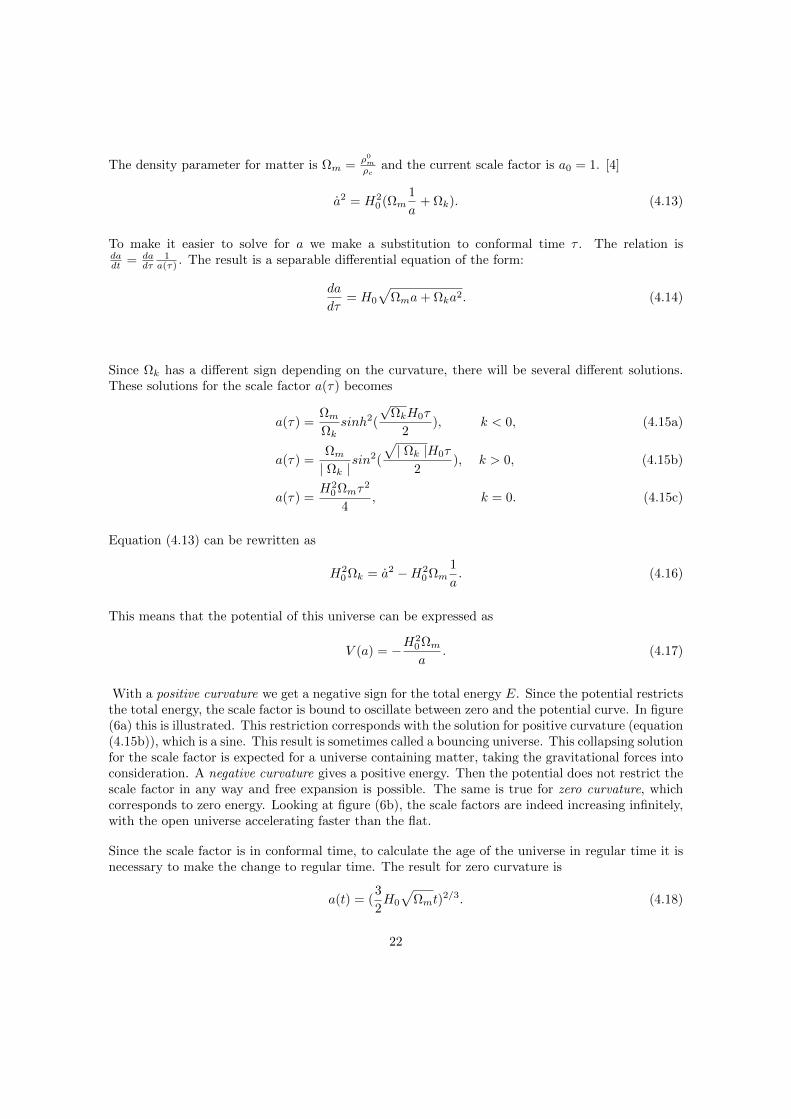
With a positive curvature we get a negative sign for the total energy E. Since the potential restrictsthe total energy, the scale factor is bound to oscillate between zero and the potential curve. In figure(6a) this is illustrated. This restriction corresponds with the solution for positive curvature (equation(4.15b)), which is a sine. This result is sometimes called a bouncing universe. This collapsing solutionfor the scale factor is expected for a universe containing matter, taking the gravitational forces intoconsideration. A negative curvature gives a positive energy. Then the potential does not restrict thescale factor in any way and free expansion is possible. The same is true for zero curvature, whichcorresponds to zero energy. Looking at figure (6b), the scale factors are indeed increasing infinitely,with the open universe accelerating faster than the flat.

Since the scale factor is in conformal time, to calculate the age of the universe in regular time it isnecessary to make the change to regular time. The result for zero curvature is

a(t) = (3

2H0

√Ωmt)

2/3. (4.18)

22

(a) Potential energy and different values for totalenergy.

(b) Scale factor for different curvatures.

Figure 6: Universe with only matter.

Using the cosmic sum Ωm = 1 and the age of the universe becomes

t =2

3H0= 9.6 billion years. (4.19)

For the ”bouncing” universe with positive curvature it is possible to calculate the period of the sinefunction. This will give the lifetime of the universe. Using the cosmic sum and the current value forΩm gives a lifetime of 17.5 billion years before collapse.

4.3 Universe With Only Radiation

For a case where the universe only consists of radiation, the Friedmann equation is

a2

a2=

8πG

3ρr −

k

a2. (4.20)

The relation between the energy density and the scale factor is used.

ρrρ0r

=a−4

a−40

=a4

0

a4. (4.21)

As before, we substitute and use the expression for the density parameter: in this case Ωr =ρ0r

ρc.

Again, a0 is taken to be 1.

a2 = H20 (Ωr

1

a2+ Ωk). (4.22)

This equation is, as with the case for a universe with only matter, easier to solve if the scale factor

23

a is in conformal time. The result is:

da

dτ= H0

√Ωr + Ωka2. (4.23)

The scale factors are:

a(τ) =

√ΩrΩk

sinh (H0

√Ωkτ), k < 0, (4.24a)

a(τ) =

√Ωr| Ωk |

sin (√| Ωk |H0τ), k > 0, (4.24b)

a(τ) = H0

√Ωrτ k = 0. (4.24c)

The potential can be obtained from equation (4.22).

V = −H20 Ωra2

. (4.25)

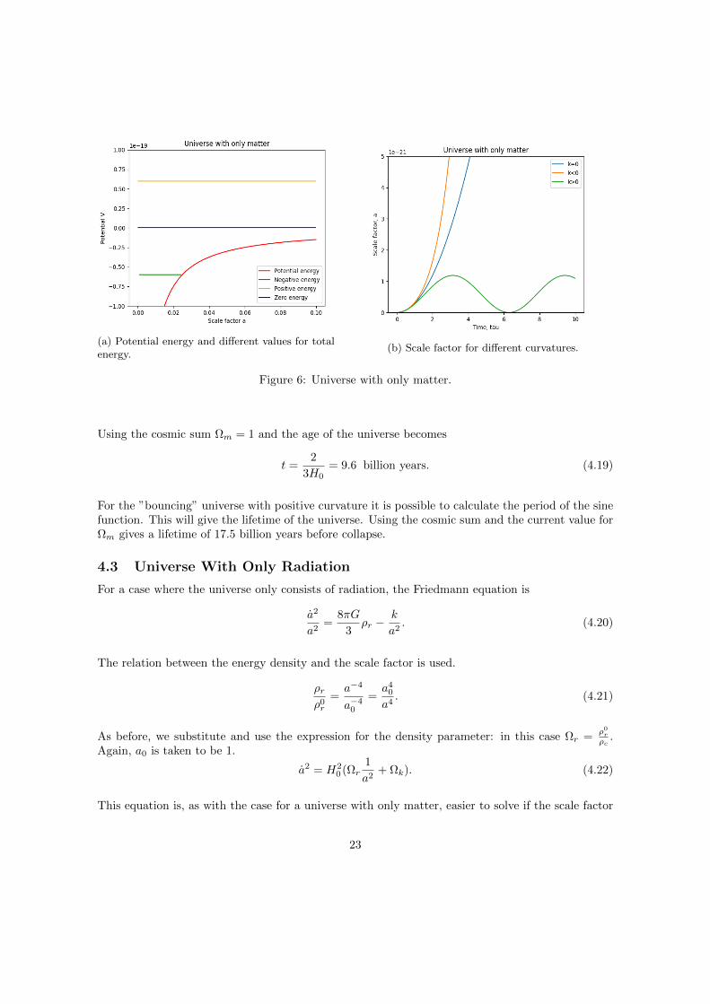
This is similar to the case of a universe which solely contains matter. Although due to the lack of a

(a) Potential energy. (b) Scale factor for different curvatures.

Figure 7: Universe with only radiation.

square of the sine we will not get a bouncing universe for a positive k. Since a(τ) can’t be negativethe scale factor will increase and decrease just once. Making a comparison of the matter andradiation universe potential for negative energy, the scale factor of the radiation dominated universeis restricted to a smaller value than the matter dominated counterpart. This is in agreement withthe graphs of the scale factors, the k > 0 graph in figure (6b) seems to have its maximum at around1 while the maximum of the k > 0 graph in figure (7b) is less than 1

2 . The age of the universe for theuniverse with zero curvature is calculated with the same method as in the previous section. Again

24

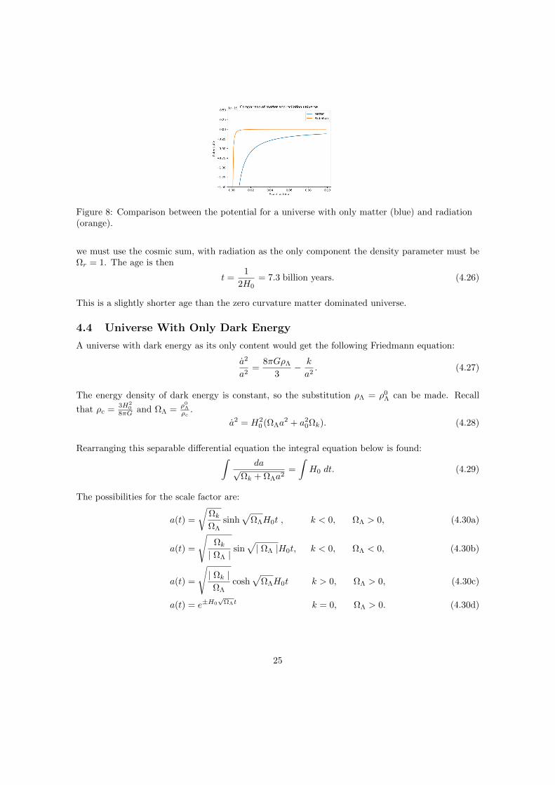
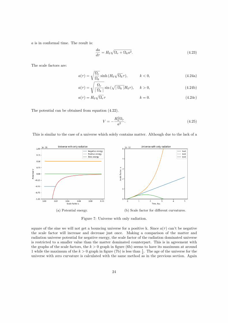
Figure 8: Comparison between the potential for a universe with only matter (blue) and radiation(orange).

we must use the cosmic sum, with radiation as the only component the density parameter must beΩr = 1. The age is then

t =1

2H0= 7.3 billion years. (4.26)

This is a slightly shorter age than the zero curvature matter dominated universe.

4.4 Universe With Only Dark Energy

A universe with dark energy as its only content would get the following Friedmann equation:

a2

a2=

8πGρΛ

3− k

a2. (4.27)

The energy density of dark energy is constant, so the substitution ρΛ = ρ0Λ can be made. Recall

that ρc =3H2

0

8πG and ΩΛ =ρ0

Λ

ρc.

a2 = H20 (ΩΛa

2 + a20Ωk). (4.28)

Rearranging this separable differential equation the integral equation below is found:∫da√

Ωk + ΩΛa2=

∫H0 dt. (4.29)

The possibilities for the scale factor are:

a(t) =

√ΩkΩΛ

sinh√

ΩΛH0t , k < 0, ΩΛ > 0, (4.30a)

a(t) =

√Ωk| ΩΛ |

sin√| ΩΛ |H0t, k < 0, ΩΛ < 0, (4.30b)

a(t) =

√| Ωk |ΩΛ

cosh√

ΩΛH0t k > 0, ΩΛ > 0, (4.30c)

a(t) = e±H0

√ΩΛt k = 0, ΩΛ > 0. (4.30d)

25

The potential energy is attained in the same way as the previous universes. It is

V = −H20 ΩΛa

2. (4.31)

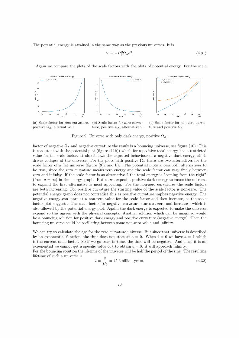
Again we compare the plots of the scale factors with the plots of potential energy. For the scale

(a) Scale factor for zero curvature,positive ΩΛ, alternative 1.

(b) Scale factor for zero curva-ture, positive ΩΛ, alternative 2.

(c) Scale factor for non-zero curva-ture and positive ΩΛ.

Figure 9: Universe with only dark energy, positive ΩΛ.

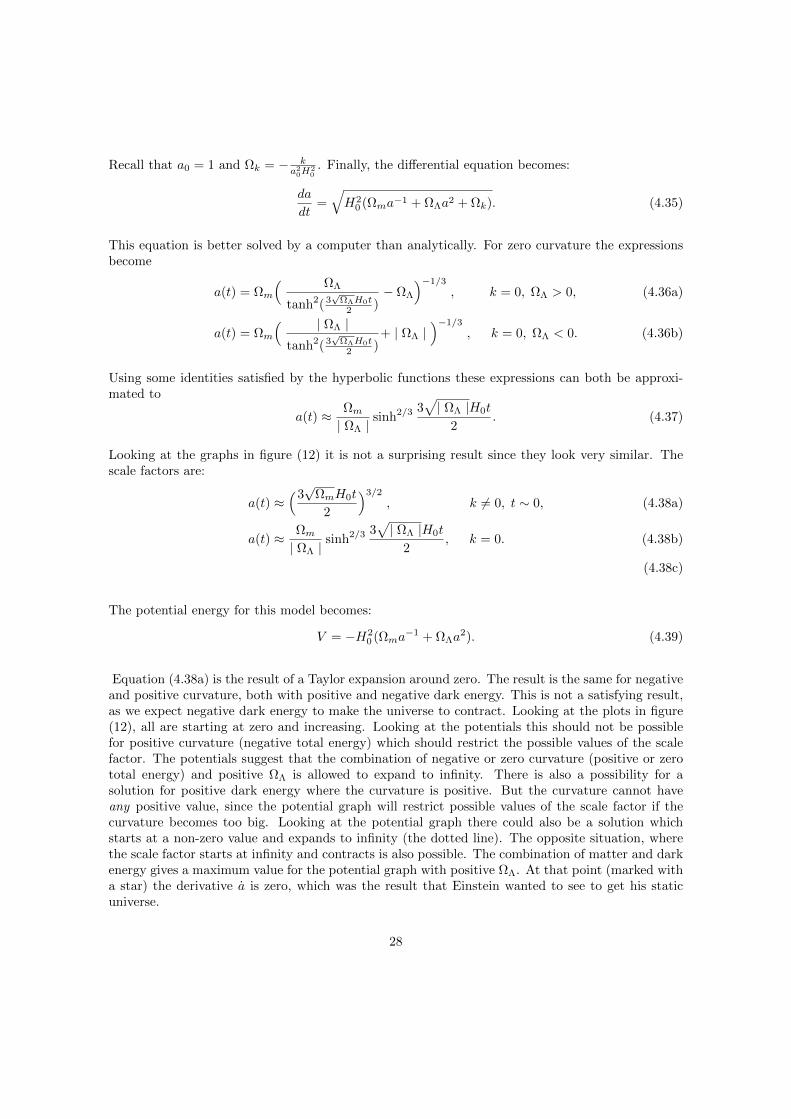
factor of negative ΩΛ and negative curvature the result is a bouncing universe, see figure (10). Thisis consistent with the potential plot (figure (11b)) which for a positive total energy has a restrictedvalue for the scale factor. It also follows the expected behaviour of a negative dark energy whichdrives collapse of the universe. For the plots with positive ΩΛ there are two alternatives for thescale factor of a flat universe (figure (9)a and b)). The potential plots allows both alternatives tobe true, since the zero curvature means zero energy and the scale factor can vary freely betweenzero and infinity. If the scale factor is as alternative 2 the total energy is ”coming from the right”(from a = ∞) in the energy graph. But as we expect a positive dark energy to cause the universeto expand the first alternative is most appealing. For the non-zero curvatures the scale factorsare both increasing. For positive curvature the starting value of the scale factor is non-zero. Thepotential energy graph does not contradict this as positive curvature implies negative energy. Thenegative energy can start at a non-zero value for the scale factor and then increase, as the scalefactor plot suggests. The scale factor for negative curvature starts at zero and increases, which isalso allowed by the potential energy plot. Again, the dark energy is expected to make the universeexpand so this agrees with the physical concepts. Another solution which can be imagined wouldbe a bouncing solution for positive dark energy and positive curvature (negative energy). Then thebouncing universe could be oscillating between some non-zero value and infinity.

We can try to calculate the age for the zero curvature universe. But since that universe is describedby an exponential function, the time does not start at a = 0. When t = 0 we have a = 1 whichis the current scale factor. So if we go back in time, the time will be negative. And since it is anexponential we cannot get a specific value of t to obtain a = 0. it will approach infinity.For the bouncing solution the lifetime of the universe will be half the period of the sine. The resultinglifetime of such a universe is

t =π

H0= 45.6 billion years. (4.32)

26

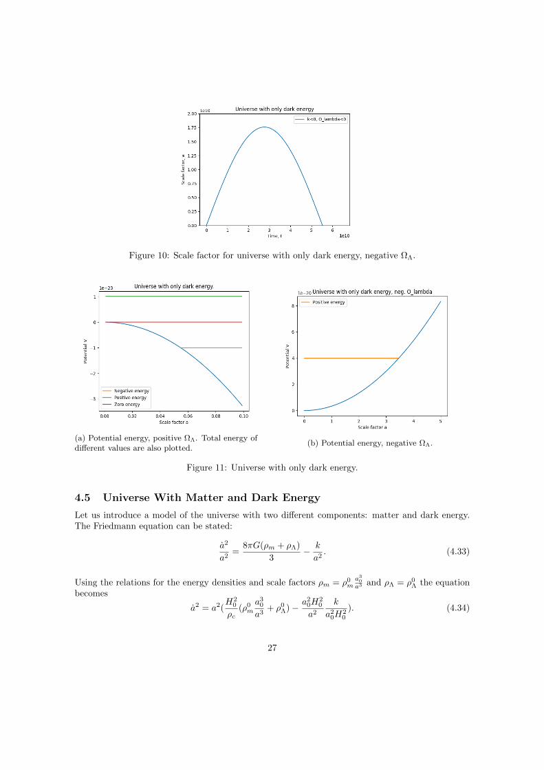
Figure 10: Scale factor for universe with only dark energy, negative ΩΛ.

(a) Potential energy, positive ΩΛ. Total energy ofdifferent values are also plotted.

(b) Potential energy, negative ΩΛ.

Figure 11: Universe with only dark energy.

4.5 Universe With Matter and Dark Energy

Let us introduce a model of the universe with two different components: matter and dark energy.The Friedmann equation can be stated:

a2

a2=

8πG(ρm + ρΛ)

3− k

a2. (4.33)

Using the relations for the energy densities and scale factors ρm = ρ0ma3

0

a3 and ρΛ = ρ0Λ the equation

becomes

a2 = a2(H2

0

ρc(ρ0m

a30

a3+ ρ0

Λ)− a20H

20

a2

k

a20H

20

). (4.34)

27

Recall that a0 = 1 and Ωk = − ka2

0H20

. Finally, the differential equation becomes:

da

dt=√H2

0 (Ωma−1 + ΩΛa2 + Ωk). (4.35)

This equation is better solved by a computer than analytically. For zero curvature the expressionsbecome

a(t) = Ωm

( ΩΛ

tanh2( 3√

ΩΛH0t2 )

− ΩΛ

)−1/3

, k = 0, ΩΛ > 0, (4.36a)

a(t) = Ωm

( | ΩΛ |tanh2( 3

√ΩΛH0t

2 )+ | ΩΛ |

)−1/3

, k = 0, ΩΛ < 0. (4.36b)

Using some identities satisfied by the hyperbolic functions these expressions can both be approxi-mated to

a(t) ≈ Ωm| ΩΛ |

sinh2/3 3√| ΩΛ |H0t

2. (4.37)

Looking at the graphs in figure (12) it is not a surprising result since they look very similar. Thescale factors are:

a(t) ≈(3√

ΩmH0t

2

)3/2

, k 6= 0, t ∼ 0, (4.38a)

a(t) ≈ Ωm| ΩΛ |

sinh2/3 3√| ΩΛ |H0t

2, k = 0. (4.38b)

(4.38c)

The potential energy for this model becomes:

V = −H20 (Ωma

−1 + ΩΛa2). (4.39)

Equation (4.38a) is the result of a Taylor expansion around zero. The result is the same for negativeand positive curvature, both with positive and negative dark energy. This is not a satisfying result,as we expect negative dark energy to make the universe to contract. Looking at the plots in figure(12), all are starting at zero and increasing. Looking at the potentials this should not be possiblefor positive curvature (negative total energy) which should restrict the possible values of the scalefactor. The potentials suggest that the combination of negative or zero curvature (positive or zerototal energy) and positive ΩΛ is allowed to expand to infinity. There is also a possibility for asolution for positive dark energy where the curvature is positive. But the curvature cannot haveany positive value, since the potential graph will restrict possible values of the scale factor if thecurvature becomes too big. Looking at the potential graph there could also be a solution whichstarts at a non-zero value and expands to infinity (the dotted line). The opposite situation, wherethe scale factor starts at infinity and contracts is also possible. The combination of matter and darkenergy gives a maximum value for the potential graph with positive ΩΛ. At that point (marked witha star) the derivative a is zero, which was the result that Einstein wanted to see to get his staticuniverse.

28

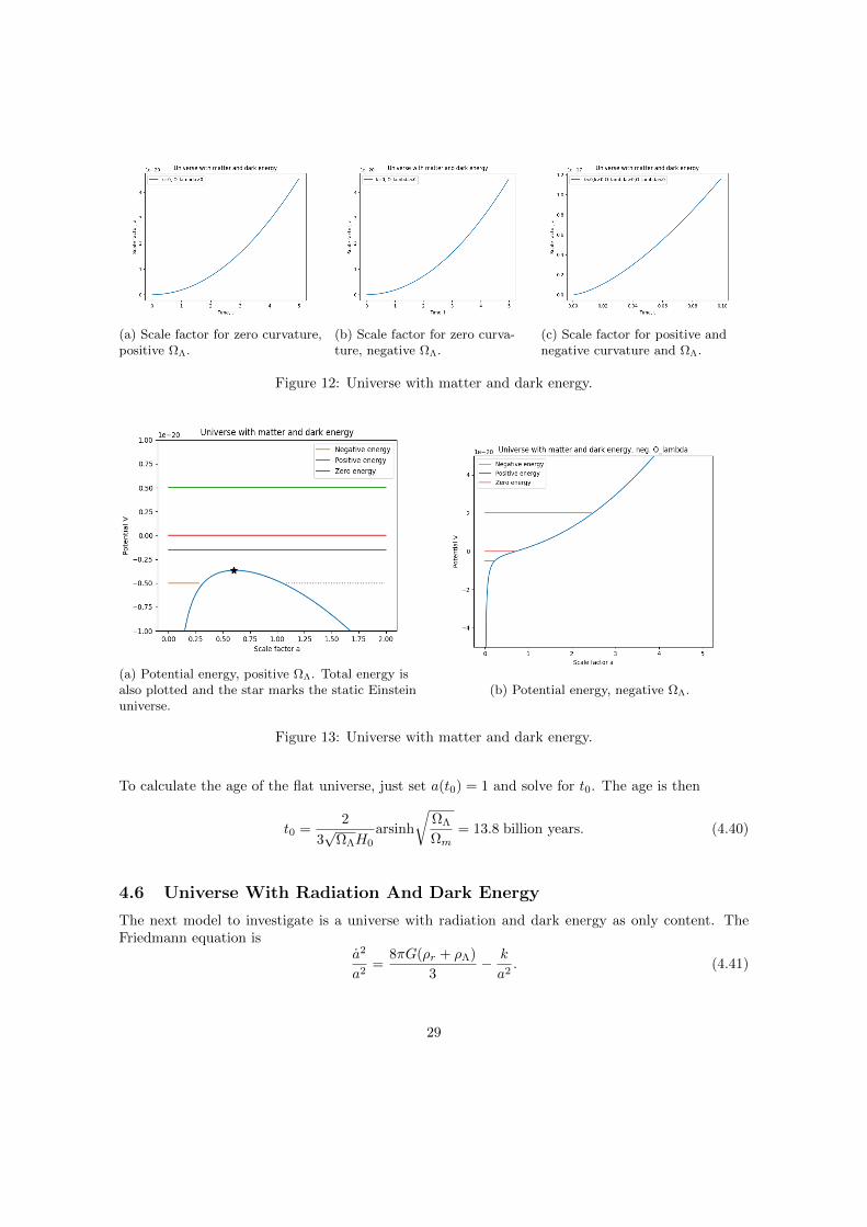
(a) Scale factor for zero curvature,positive ΩΛ.

(b) Scale factor for zero curva-ture, negative ΩΛ.

(c) Scale factor for positive andnegative curvature and ΩΛ.

Figure 12: Universe with matter and dark energy.

(a) Potential energy, positive ΩΛ. Total energy isalso plotted and the star marks the static Einsteinuniverse.

(b) Potential energy, negative ΩΛ.

Figure 13: Universe with matter and dark energy.

To calculate the age of the flat universe, just set a(t0) = 1 and solve for t0. The age is then

t0 =2

3√

ΩΛH0

arsinh

√ΩΛ

Ωm= 13.8 billion years. (4.40)

4.6 Universe With Radiation And Dark Energy

The next model to investigate is a universe with radiation and dark energy as only content. TheFriedmann equation is

a2

a2=

8πG(ρr + ρΛ)

3− k

a2. (4.41)

29

Again, it is possible to make use of the relation between the scale factor and the energy density andsubstitute. The density parameter relations are utilized as well.

a2 = H20 (

Ωra2

+ ΩΛa2 + Ωk). (4.42)

The resulting separable differential equation can be solved integrating and choosing appropriatesubstitutions. The solutions for the scale factors are:

a(t) =

√√Ω2k

4+ ΩrΩΛ sin (2

√ΩΛH0t) +

Ωk

2√

ΩΛ

k 6= 0, ΩΛ < 0, (4.43a)

a(t) =

√√ΩrΩΛ

sinh (2√

ΩΛH0t) , k = 0, ΩΛ > 0, (4.43b)

a(t) =

√√√√√ Ωr| ΩΛ |

sin (2√| ΩΛ |H0t) , k = 0, ΩΛ < 0. (4.43c)

The potential energy is:

V = −H20 (

Ωra2

+ ΩΛa2). (4.44)

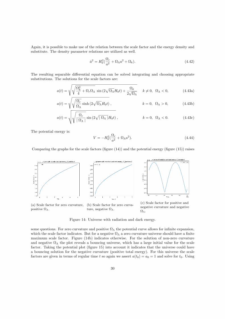
Comparing the graphs for the scale factors (figure (14)) and the potential energy (figure (15)) raises

(a) Scale factor for zero curvature,positive ΩΛ.

(b) Scale factor for zero curva-ture, negative ΩΛ.

(c) Scale factor for positive andnegative curvature and negativeΩΛ.

Figure 14: Universe with radiation and dark energy.

some questions. For zero curvature and positive ΩΛ the potential curve allows for infinite expansion,which the scale factor indicates. But for a negative ΩΛ a zero curvature universe should have a finitemaximum scale factor. Figure (14b) indicates otherwise. For the solution of non-zero curvatureand negative ΩΛ the plot reveals a bouncing universe, which has a large initial value for the scalefactor. Taking the potential plot (figure 15) into account it indicates that the universe could havea bouncing solution for the negative curvature (positive total energy). For this universe the scalefactors are given in terms of regular time t so again we assert a(t0) = a0 = 1 and solve for t0. Using

30

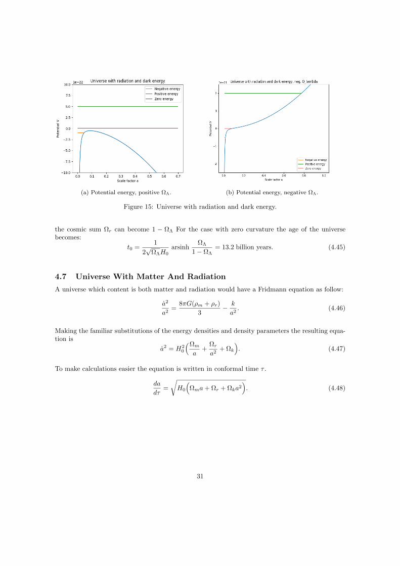
(a) Potential energy, positive ΩΛ. (b) Potential energy, negative ΩΛ.

Figure 15: Universe with radiation and dark energy.

the cosmic sum Ωr can become 1 − ΩΛ For the case with zero curvature the age of the universebecomes:

t0 =1

2√

ΩΛH0

arsinhΩΛ

1− ΩΛ= 13.2 billion years. (4.45)

4.7 Universe With Matter And Radiation

A universe which content is both matter and radiation would have a Fridmann equation as follow:

a2

a2=

8πG(ρm + ρr)

3− k

a2. (4.46)

Making the familiar substitutions of the energy densities and density parameters the resulting equa-tion is

a2 = H20

(Ωma

+Ωra2

+ Ωk

). (4.47)

To make calculations easier the equation is written in conformal time τ .

da

dτ=

√H0

(Ωma+ Ωr + Ωka2

). (4.48)

31

Solving the equations give the following scale factors:

a(t) =1√Ωk

(√Ωr −

Ω2m

4Ωksinh

√ΩkH0τ −

Ωm

2√

Ωk

)k < 0, (4.49a)

a(t) =1√Ωk

(√Ωr +

Ω2m

4Ωksin√

ΩkH0τ +Ωm

2√

Ωk

), k > 0, (4.49b)

a(t) =ΩmH

20 τ

2

4− Ωr

Ωm, k = 0. (4.49c)

The potential energy is:

V = −H20 (

Ωma

+Ωra2

). (4.50)

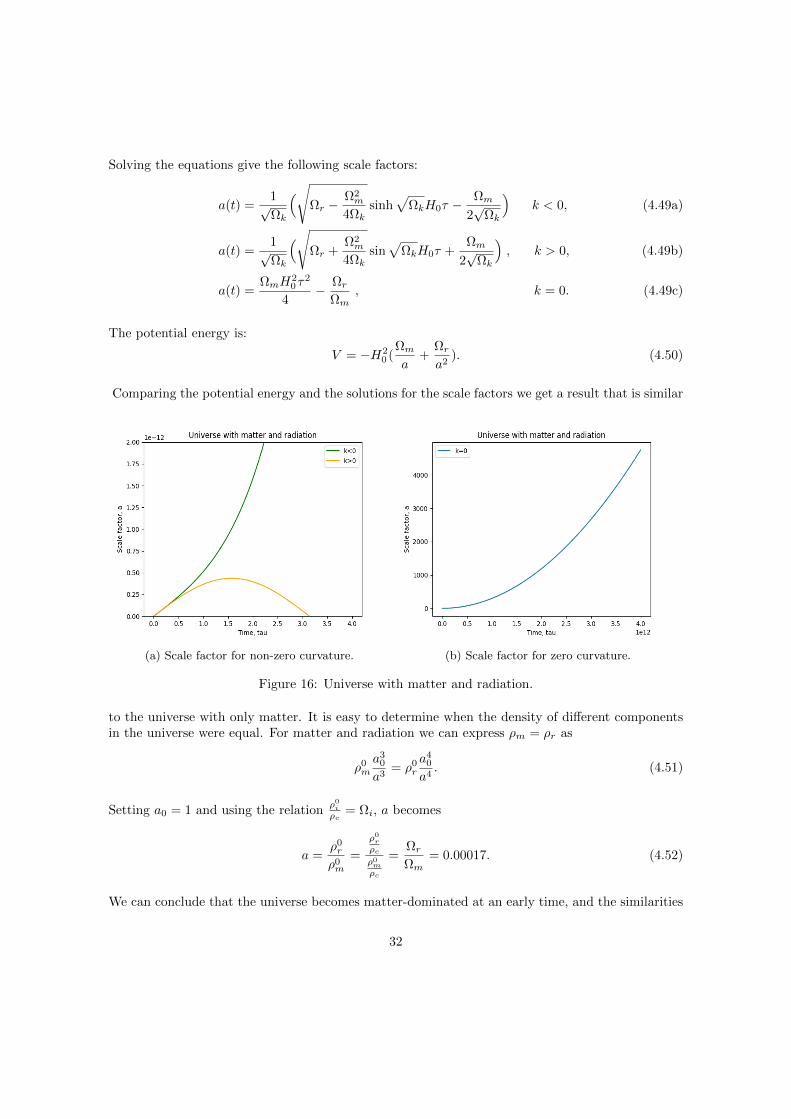
Comparing the potential energy and the solutions for the scale factors we get a result that is similar

(a) Scale factor for non-zero curvature. (b) Scale factor for zero curvature.

Figure 16: Universe with matter and radiation.

to the universe with only matter. It is easy to determine when the density of different componentsin the universe were equal. For matter and radiation we can express ρm = ρr as

ρ0m

a30

a3= ρ0

r

a40

a4. (4.51)

Setting a0 = 1 and using the relationρ0i

ρc= Ωi, a becomes

a =ρ0r

ρ0m

=

ρ0r

ρcρ0m

ρc

=ΩrΩm

= 0.00017. (4.52)

We can conclude that the universe becomes matter-dominated at an early time, and the similarities

32

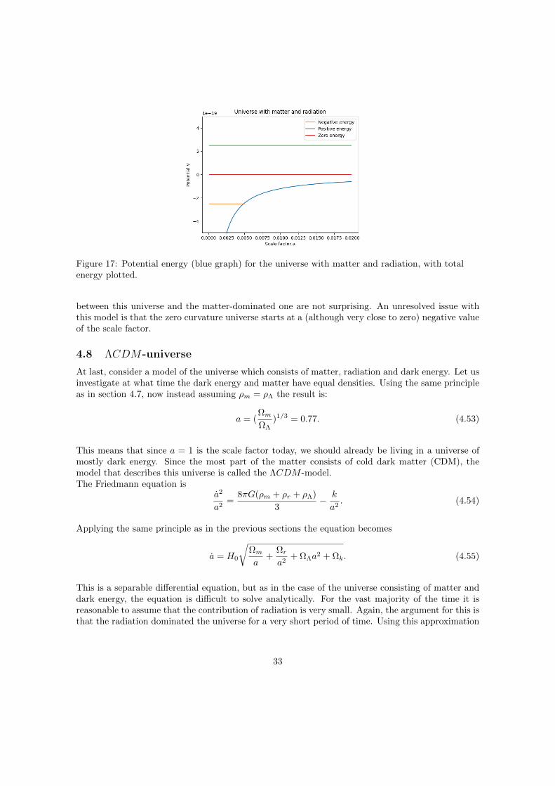
Figure 17: Potential energy (blue graph) for the universe with matter and radiation, with totalenergy plotted.

between this universe and the matter-dominated one are not surprising. An unresolved issue withthis model is that the zero curvature universe starts at a (although very close to zero) negative valueof the scale factor.

4.8 ΛCDM-universe

At last, consider a model of the universe which consists of matter, radiation and dark energy. Let usinvestigate at what time the dark energy and matter have equal densities. Using the same principleas in section 4.7, now instead assuming ρm = ρΛ the result is:

a = (ΩmΩΛ

)1/3 = 0.77. (4.53)

This means that since a = 1 is the scale factor today, we should already be living in a universe ofmostly dark energy. Since the most part of the matter consists of cold dark matter (CDM), themodel that describes this universe is called the ΛCDM -model.The Friedmann equation is

a2

a2=

8πG(ρm + ρr + ρΛ)

3− k

a2. (4.54)

Applying the same principle as in the previous sections the equation becomes

a = H0

√Ωma

+Ωra2

+ ΩΛa2 + Ωk. (4.55)

This is a separable differential equation, but as in the case of the universe consisting of matter anddark energy, the equation is difficult to solve analytically. For the vast majority of the time it isreasonable to assume that the contribution of radiation is very small. Again, the argument for this isthat the radiation dominated the universe for a very short period of time. Using this approximation

33

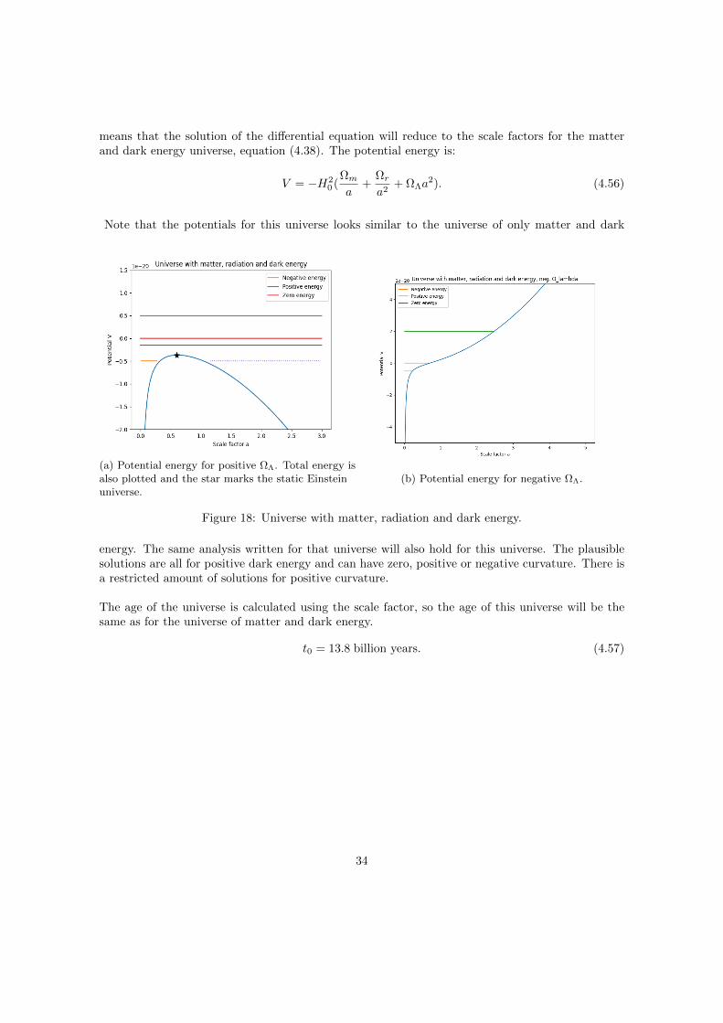
means that the solution of the differential equation will reduce to the scale factors for the matterand dark energy universe, equation (4.38). The potential energy is:

V = −H20 (

Ωma

+Ωra2

+ ΩΛa2). (4.56)

Note that the potentials for this universe looks similar to the universe of only matter and dark

(a) Potential energy for positive ΩΛ. Total energy isalso plotted and the star marks the static Einsteinuniverse.

(b) Potential energy for negative ΩΛ.

Figure 18: Universe with matter, radiation and dark energy.

energy. The same analysis written for that universe will also hold for this universe. The plausiblesolutions are all for positive dark energy and can have zero, positive or negative curvature. There isa restricted amount of solutions for positive curvature.

The age of the universe is calculated using the scale factor, so the age of this universe will be thesame as for the universe of matter and dark energy.

t0 = 13.8 billion years. (4.57)

34

5 Conclusion

In this thesis the dynamics of universes have been explored. General relativity has been used as atool to understand what would happen in different cosmological models. The framework of generalrelativity has allowed us to enter the physical world of curvature. It connects the properties of matter,such as the energy and momentum, to the geometry of the space which it inhabits. We now knowthat gravitation and curvature are intertwined and cannot be handled separately. The relationbetween the geometry of space and its content is described by the Einstein equation. The basicfoundations of cosmology have been covered, describing how current cosmological models describeour Universe. We seem to live in a homogeneous universe, characterized by its isotropic smoothness.It is the cosmological principle that tells us that no matter where we look in the universe we willsee more or less the same things. Making use of these assumptions the Einstein equation can besolved in a neat way. The result is the Friedmann equation, which describes the relation betweenthe density distribution and the geometrical behaviour of the universe. Will the universe collapse?Or perhaps expand indefinitely? The answers to these questions are governed by the Friedmannequation.

Different hypothetical universes have been investigated by solving the Friedmann equation for variouscases. We have learned that both matter and negative dark energy can drive universes to collapse.The positive dark energy on the other hand affects the universe in the opposite way, making itexpand. Radiation does not have a substantial effect on the fate of the universe. The curvatureleads in many cases to diametrically opposed consequences for the universes, so it is of importance.When we explore the ΛCDM-universe which contains all three components, it is sufficient to onlytake matter and dark energy into account. The ΛCDM-universe gives the most detailed description ofour Universe provided in this thesis. For this case the solutions suggest a flat, closed or open universewhich is expanding, with some restrictions for the maximum curvature of the closed universe.

The results in this thesis is based of the value of the Hubble constant. The increasing tensionbetween the different values of the constant is of course affecting the reliability of the report. Itwill be fascinating to see what lies ahead in cosmology research, as our Universe holds many moremysteries to uncover.

35

Appendix

Let us introduce an interval which is parameterized by the time- and radius dependent functionsf(t) and g(r).

ds2 = −dt2 + f(t)(g(r)dr2 + r2dθ2 + r2 sin2 θdφ2

)(.1)

The associated metric tensor can be represented by matrices as showed below, where gtt = g00 = −1,grr = g11 = fg and so on.

gµν =

−1 0 0 00 fg 0 00 0 fr2 00 0 0 fr2 sin2 θ

gµν =

−1 0 0 00 1

fg 0 0

0 0 1fr2 0

0 0 0 1fr2 sin2 θ

(.2)

Our goal is to calculate the non-zero Riemann tensor components of this metric, and then find theRicci tensor components and Ricci scalar. To calculate the Riemann tensors the Christoffel symbolsare needed. The Christoffel symbols can be obtained using the following expression.

Γσµν =1

2gρσ(

∂gνρ∂xµ

+∂gµρ∂xν

− ∂gνµ∂xρ

). (.3)

This can be written more efficiently with ∂∂xµ = ∂µ.

Γσµν =1

2gρσ(∂µgνρ + ∂νgµρ − ∂ρgνµ

)(.4)

Many Christoffel symbols will vanish, only the ones with at least two repeated indices can give anon-zero value. Starting with Γ0

11, will give the following expression.

Γ011 =

1

2gρ0(∂1g1ρ + ∂1g1ρ − ∂ρg11

)(.5)

Now the index ρ will be repeated for all possible coordinate variables (t, r, θ and φ). But sincethe chosen metric tensor is symmetric, we can deduce that ρ = 0 will be the only surviving term.Substituting ρ and eliminating terms with non-repeated indices we obtain:

Γ011 =

1

2g00(∂1g10 + ∂1g10 − ∂ρg11

)=

1

2g00(− ∂0g11

). (.6)

The next step is to substitute the metric components and perform the derivative.

Γ011 =

1

2(−1)

(− ∂0(fg)

)=gf

2(.7)

Now that we have described this method in a detailed way it only remains to do exactly the same

36

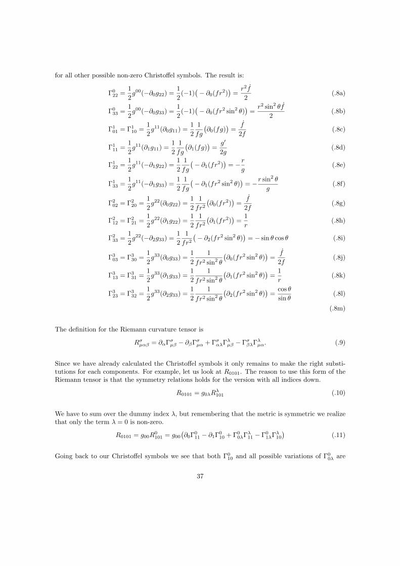
for all other possible non-zero Christoffel symbols. The result is:

Γ022 =

1

2g00(−∂0g22) =

1

2(−1)

(− ∂0(fr2)

)=r2f

2(.8a)

Γ033 =

1

2g00(−∂0g33) =

1

2(−1)

(− ∂0(fr2 sin2 θ)

)=r2 sin2 θf

2(.8b)

Γ101 = Γ1

10 =1

2g11(∂0g11) =

1

2

1

fg

(∂0(fg)

)=

f

2f(.8c)

Γ111 =

1

2g11(∂1g11) =

1

2

1

fg

(∂1(fg)

)=g′

2g(.8d)

Γ122 =

1

2g11(−∂1g22) =

1

2

1

fg

(− ∂1(fr2)

)= − r

g(.8e)

Γ133 =

1

2g11(−∂1g33) =

1

2

1

fg

(− ∂1(fr2 sin2 θ)

)= −r sin2 θ

g(.8f)

Γ202 = Γ2

20 =1

2g22(∂0g22) =

1

2

1

fr2

(∂0(fr2)

)=

f

2f(.8g)

Γ212 = Γ2

21 =1

2g22(∂1g22) =

1

2

1

fr2

(∂1(fr2)

)=

1

r(.8h)

Γ233 =

1

2g22(−∂2g33) =

1

2

1

fr2

(− ∂2(fr2 sin2 θ)

)= − sin θ cos θ (.8i)

Γ303 = Γ3

30 =1

2g33(∂0g33) =

1

2

1

fr2 sin2 θ

(∂0(fr2 sin2 θ)

)=

f

2f(.8j)

Γ313 = Γ3

31 =1

2g33(∂1g33) =

1

2

1

fr2 sin2 θ

(∂1(fr2 sin2 θ)

)=

1

r(.8k)

Γ323 = Γ3

32 =1

2g33(∂2g33) =

1

2

1

fr2 sin2 θ

(∂2(fr2 sin2 θ)

)=

cos θ

sin θ(.8l)

(.8m)

The definition for the Riemann curvature tensor is

Rσµαβ = ∂αΓσµβ − ∂βΓσµα + ΓσαλΓλµβ − ΓσβλΓλµα. (.9)

Since we have already calculated the Christoffel symbols it only remains to make the right substi-tutions for each components. For example, let us look at R0101. The reason to use this form of theRiemann tensor is that the symmetry relations holds for the version with all indices down.

R0101 = g0λRλ101 (.10)

We have to sum over the dummy index λ, but remembering that the metric is symmetric we realizethat only the term λ = 0 is non-zero.

R0101 = g00R0101 = g00

(∂0Γ0

11 − ∂1Γ010 + Γ0

0λΓλ11 − Γ01λΓλ10

)(.11)

Going back to our Christoffel symbols we see that both Γ010 and all possible variations of Γ0

0λ are

37

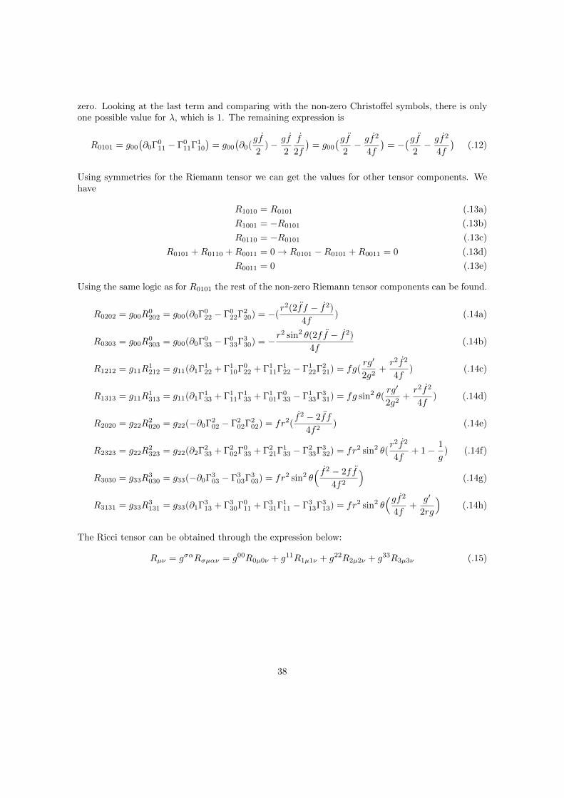
zero. Looking at the last term and comparing with the non-zero Christoffel symbols, there is onlyone possible value for λ, which is 1. The remaining expression is

R0101 = g00

(∂0Γ0

11 − Γ011Γ1

10

)= g00

(∂0(

gf

2)− gf

2

f

2f

)= g00

(gf2− gf2

4f

)= −

(gf2− gf2

4f

)(.12)

Using symmetries for the Riemann tensor we can get the values for other tensor components. Wehave

R1010 = R0101 (.13a)

R1001 = −R0101 (.13b)

R0110 = −R0101 (.13c)

R0101 +R0110 +R0011 = 0→ R0101 −R0101 +R0011 = 0 (.13d)

R0011 = 0 (.13e)

Using the same logic as for R0101 the rest of the non-zero Riemann tensor components can be found.

R0202 = g00R0202 = g00(∂0Γ0

22 − Γ022Γ2

20) = −(r2(2ff − f2)

4f) (.14a)

R0303 = g00R0303 = g00(∂0Γ0

33 − Γ033Γ3

30) = −r2 sin2 θ(2ff − f2)

4f(.14b)

R1212 = g11R1212 = g11(∂1Γ1

22 + Γ110Γ0

22 + Γ111Γ1

22 − Γ122Γ2

21) = fg(rg′

2g2+r2f2

4f) (.14c)

R1313 = g11R1313 = g11(∂1Γ1

33 + Γ111Γ1

33 + Γ101Γ0

33 − Γ133Γ3

31) = fg sin2 θ(rg′

2g2+r2f2

4f) (.14d)

R2020 = g22R2020 = g22(−∂0Γ2

02 − Γ202Γ2

02) = fr2(f2 − 2ff

4f2) (.14e)

R2323 = g22R2323 = g22(∂2Γ2

33 + Γ202Γ0

33 + Γ221Γ1

33 − Γ233Γ3

32) = fr2 sin2 θ(r2f2

4f+ 1− 1

g) (.14f)

R3030 = g33R3030 = g33(−∂0Γ3

03 − Γ303Γ3

03) = fr2 sin2 θ( f2 − 2ff

4f2

)(.14g)

R3131 = g33R3131 = g33(∂1Γ3

13 + Γ330Γ0

11 + Γ331Γ1

11 − Γ313Γ3

13) = fr2 sin2 θ(gf2

4f+

g′

2rg

)(.14h)

The Ricci tensor can be obtained through the expression below:

Rµν = gσαRσµαν = g00R0µ0ν + g11R1µ1ν + g22R2µ2ν + g33R3µ3ν (.15)

38

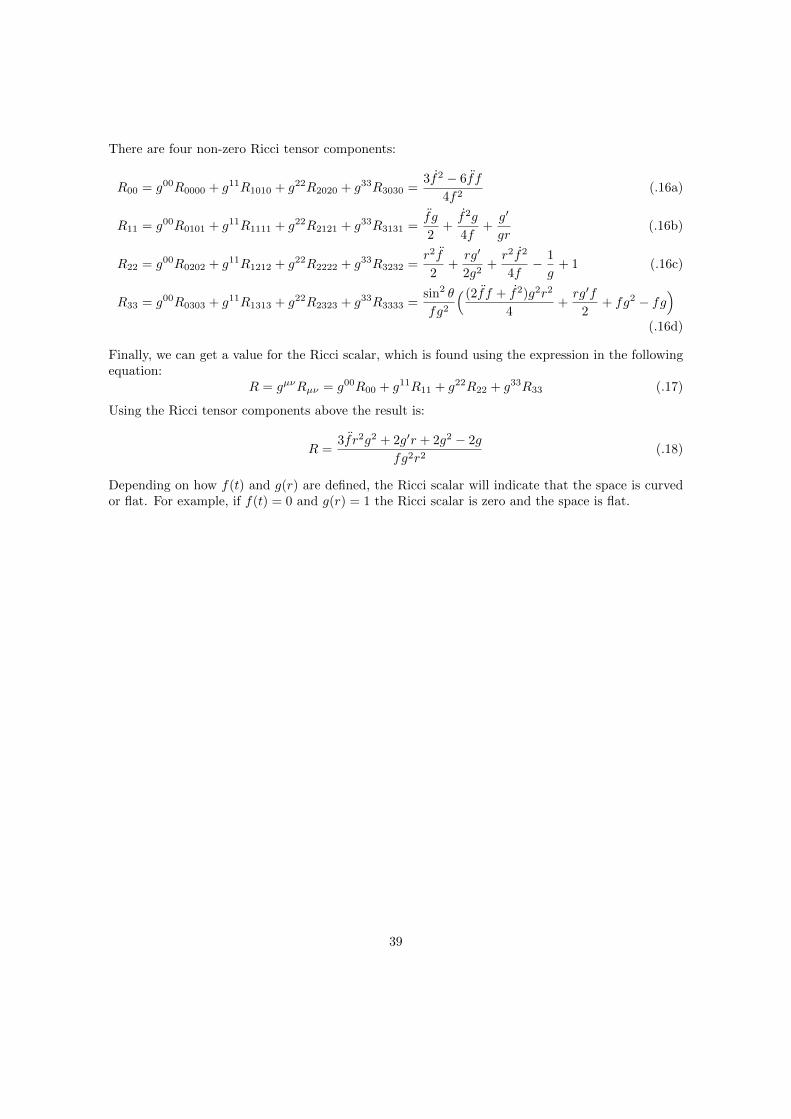
There are four non-zero Ricci tensor components:

R00 = g00R0000 + g11R1010 + g22R2020 + g33R3030 =3f2 − 6ff

4f2(.16a)

R11 = g00R0101 + g11R1111 + g22R2121 + g33R3131 =fg

2+f2g

4f+g′

gr(.16b)

R22 = g00R0202 + g11R1212 + g22R2222 + g33R3232 =r2f

2+rg′

2g2+r2f2

4f− 1

g+ 1 (.16c)

R33 = g00R0303 + g11R1313 + g22R2323 + g33R3333 =sin2 θ

fg2

( (2ff + f2)g2r2

4+rg′f

2+ fg2 − fg

)(.16d)

Finally, we can get a value for the Ricci scalar, which is found using the expression in the followingequation:

R = gµνRµν = g00R00 + g11R11 + g22R22 + g33R33 (.17)

Using the Ricci tensor components above the result is:

R =3f r2g2 + 2g′r + 2g2 − 2g

fg2r2(.18)

Depending on how f(t) and g(r) are defined, the Ricci scalar will indicate that the space is curvedor flat. For example, if f(t) = 0 and g(r) = 1 the Ricci scalar is zero and the space is flat.

39

References

[1] H.S. Kragh. “Conceptions of Cosmos : From Myths to the Accelerating Universe: a History ofCosmology”. In: Oxford University Press, Oxford, 2007.

[2] S. Weinberg. “Gravitation and cosmology: principles and applications of the general theory ofrelativity”. In: Wiley, New York, 1972.

[3] A. Einstein. “The field equations of gravitation”. In: Sitzungsberichte der Koniglich Preußis-chen Akademie der Wissenschaften. Berlin (Math. Phys.) 1915 (1915), pp. 844–847.

[4] A. Liddle. “An Introduction to Modern Cosmology”. In: John Wiley and Sons, Chichester,2015.

[5] B.F. Schutz. “A First Course in General Relativity”. In: Cambridge University Press, Cam-bridge, 2009.

[6] S.M. Carroll. “Spacetime and Geometry : An Introduction to General Relativity”. In: Pearson,Harlow, 2004.

[7] L. Bergstrom. “Cosmology and Particle Astrophysics”. In: Springer, Berlin, 2004.

[8] V. Mukhanov. “Physical Foundations of Cosmology”. In: Cambridge University Press, Cam-bridge, 2005.

[9] Scott. Dodelson. “Modern Physics”. In: Academic Press, 2020.

[10] Nobel Prize Committee. All Nobel Prizes in Physics. url: https://www.nobelprize.org/prizes/lists/all-nobel-prizes-in-physics/. (accessed: 2021-06-01).

[11] N. Aghanim et al. “Planck 2018 results. VI. Cosmological parameters”. In: Astronomy andAstrophysics, 2020.

[12] A.G. Riess et al. “Cosmic Distances Calibrated to 1 % Precision with Gaia EDR3 Parallaxesand Hubble Space Telescope Photometry of 75 Milky Way Cepheids Confirm Tension with ΛCDM”. In: Astrophysical journal. 908.1 (2021), p. L6. doi: 10.3847/2041-8213/abdbaf.

[13] E. Di Valentino et al. In the Realm of the Hubble tension - a Review of Solutions. url: https://arxiv.org/pdf/2103.01183.pdf. (accessed: 2021-06-07).

40