Embed Size (px)
DESCRIPTION
General Relativity
Citation preview
General Relativity and Cosmology 1
Lectures on General Relativity and Cosmology
Pedro G. FerreiraAstrophysics
University of Oxford,DW Building, Keble RoadOxford OX1 3RH, UK
last modified May 22, 2015
Preamble
The following set of lectures was designed for the Oxford Undergraduate course and are givenduring the 3rd year of the BA or MPhys course. I have tried to keep the mathematical jargonto a minimum and ground most of the explanations with physical examples and applications.Yet you will see that, although there is very little emphasis on differential geometry you stillhave to learn what tensors or covariant derivatives are. So be it.
These notes are not very original and are based on a number of books and lectures. Inparticular I have used
• Gravitation and Cosmology, Steven Weinberg (Wiley, 1972)
• Gravity: An Introduction to Einstein’s General Relativity, James B. Hartle (AddisonWesley, 2003)
• Part II General Relativity, G W Gibbons (can be found online onhttp://www.damtp.cam.ac.uk/research/gr/members/gibbons/partiipublic-2006.pdf)
• General Relativity: An introduction for Physicists, M.P Hobson, G.P.Efstathiou andA.N.Lasenby (CUP, 2006)
• General Relativity, Alan Heavens (not publicly available).
• Theories of Gravity and Cosmology T. Clifton, P.G. Ferreira and C. Skordis (PhysicsReports, 2012)
• Cosmological Physics John Peacock (CUP, 1998)
But there are many texts out there that you can consult.For a start, I will assume that the time coordinate, t and the spatial coordinate, ~x =
(x1, x2, x3) can be organized into a 4-vector (x0, x1, x2, x3) = (ct, ~x) where c is the speed oflight. Throughout these lecture notes I will use the (−,+,+,+) convention for the metric.This means that the Minkowski metric is a matrix of the form
ηµν =
−1 0 0 00 1 0 00 0 1 00 0 0 1
(1)
General Relativity and Cosmology 2
You will note that this is the opposite convention to the one used when you were first learningspecial relativity. In fact you will find that, in general (but not always), books on GeneralRelativity will use the convention we use here, while books on particle physics or quantum fieldtheory will use the opposite convention.
We will be using the convention that Roman labels (like i, j, etc) span 1 to 3 and labelspatial vectors while Greek labels (such as α, β, etc) span 0 to 3 and label space-time vectors.
We will also be using the Einstein summation convention. This means that, whenever wehave a pair of indices which are the same, we must add over them. So for example, when wewrite
ds2 = ηαβdxαdxβ
we mean
ds2 =3∑
α=0
3∑
β=0
ηαβdxαdxβ
Note that the paired indices always appear with one as a superscript (i.e. ”up”) and the otherone as a subscript (i.e. ”down”).
Finally, I am extremely grateful to Tessa Baker, Tim Clifton, Rosanna Hardwick, AlanHeavens, Anthony Lewis, Ed Macaulay and Patrick Timoney for their help in putting togetherthe lecture notes, exercises and spotting errors.
1 Why General Relativity?
Throughout your degree, you have learnt how almost all the laws of physics are invariant ifyou transform between inertial reference frames. With Special Relativity you can now writeNewton’s 2nd law, the conservation of energy and momentum, Maxwell’s equations, etc in a waythat they are unchanged under the Lorentz transformation. One force stands apart: gravity.Newton’s law of gravity, the inverse square law, is manifestly not invariant under the Lorentztransformation.
You can now ask yourself the question: can we write down the laws of physics so they areinvariant under any transformation? Not only between reference frames with constant velocitybut also between accelerating reference frames. It turns out that we can and in doing so, weincorporate gravity into the mix. That is what the General Theory of Relativity is about.
2 Newtonian Gravity
In these lectures we will be studying the modern view of gravity. Einstein’s theory of space-time is one of the crowning achievements of modern physics and transformed the way we thinkabout the fundamental laws of nature. It superseded a spectacularly successful theory, Newton’stheory of gravity. If we are to understand the importance and consequences of Einstein’s theory,we need to learn (or revise) the main characteristics of Newton’s theory.
General Relativity and Cosmology 3
Newton’s Law of Universal Gravitation for two bodies A and B with masses mA and mB
at a separation r can be stated in a simplified form as:
F = −GmAmB
r2
where G = 6.672× 10⁻¹¹ m3kg−1s−2. The resulting gravitational acceleration felt by mass mA
is
g = −GmB
r2
We can rewrite the expression in terms of vectors r = (x1, x2, x3).
F = GmAmBrB − rA
r3
is the force exerted on the mass mA and the gravitational acceleration
F = mAg
Consider now a few simple applications. We can use the above expression to work out thegravitational acceleration on the surface of the Earth. If we Taylor expand around the radiusof the Earth, R⊕ we find
g = −GM⊕r2
= −GM⊕
(R⊕ + h)2≃ −G
M⊕R2
⊕(1− 2
h
R⊕)
where h is the height above the surface of the Earth and M⊕ is the mass of the Earth. WithM⊕ = 5.974× 1027g and R⊕ = 6.378× 108cm we find a familiar value: g ≃ 9.8ms−2.
The power of Newton’s theory is that it allows us to describe, with tremendous accuracy,the evolution of the Solar System. To do so, we need to solve the two body problem. We havethat the equations of motion are
mirA = GmAmBrB − rA
r3
with r = |r| = |rA − rB|. We are interested in how r evolves and we can find its evolution bysimplifying this system. Let us first define the total mass
M = mA +mB
and the reduced mass
µ =mAmB
M
Ignoring the motion of the centre of mass, we have that the Lagrangian for this system will be
L =1
2µr · r+G
µM
r
General Relativity and Cosmology 4
It is more convenient to transform to spherical coordinates so
x1 = r cos(φ) sin(θ)
x2 = r sin(φ) sin(θ)
x3 = r cos(θ)
then the Lagrangian becomes
L =1
2µ(r2 + r2θ2 + r2 sin2(θ)φ2) +G
µM
r
The angular parts of the Euler-Lagrange equations are
µd
dt(r2θ) = µr2 sin(θ) cos(θ)φ2
d
dt
[
µr2 sin2(θ)φ]
= 0
We can integrate the second equation to give
µr2 sin2(θ)φ = Jφ
and, multiplying the first equation by 2r2θ, we can integrate to find
µ2r4θ2 = J2θ − J2
φ
sin2(θ)
We can now choose a coordinate system such that the orbit lies on the equatorial plane (θ = π/2)and Jθ = Jφ = J which corresponds to θ = 0. We are left with two coordinates, r and φ.
Replacing the the angular momentum conservation equation in the radial equation of mo-tion, we have
µr − J2
µr3+G
µM
r2= 0
which we can integrate to give us an expression for the conserved energy
E
µ=
1
2r2 +
1
2
J2
µ2r2−G
M
r(2)
Note that we can define an effective potential energy which is given by
Veff (r) =1
2
J2
µr2−G
µM
r
Again, using conservation of energy, we can use
Jdt = µr2dφ
to reexpress time derivatives in terms of angular derivatives
d
dt=
J
µr2d
dφand
d2
dt2=
J
µr2d
dφ(J
µr2d
dφ)
General Relativity and Cosmology 5
The Euler Lagrange equation then becomes
J
r2d
dφ
(
J
µr2dr
dφ
)
− J2
µr3= −G
µM
r2
If we change to u = 1/r we have
d2u
dφ2+ u =
µ
J2GµM (3)
This is the simple harmonic oscillator equation with a constant driving force. We can solve thisequation to find
u =1
r=
Gµ(µM)
J2
1 +
√
√
√
√1 +2EJ2
µ(GµM)2cos(φ− φ0)
where E is the conserved energy of the system (and an integration constant) and φ0 is theturning point of the orbit (and the second integration constant). You should recognize this asthe equation for a conic with ellipticity e given by
e =
√
√
√
√1 +2EJ2
µ(GµM)2
In other words, the trajectories of the two body problem correspond to closed orbits in theform of ellipses.
The Solar System is almost perfectly described in terms of these trajectories. In fact almostall the planets have quasi-circular orbits with eccentricities e ≃ 1− 10%. Mercury stands out,with e ≃ 20%. Furthermore, Mercury’s orbit does not actually close in on itself but precessesat a rate of about 5600 arc seconds per century. This primarily due to the effect of the otherplanets slowly nudging it around and, again, can be explained with Newtonian mechanics. Butsince the mid 19th century, it has been known that there is still an un accounted amount ofprecession, about 43 arc seconds per century. We shall find its origin in later lectures.
Finally, it is convenient to define the Newtonian potential or gravitational potential in termsof the potential energy, V , of the system:
V ≡ mΦ
The gravitational force will then be
F = −∇V
and the gravitational acceleration is given by
g = −∇Φ
The gravitational potential satisfies the Newton Poisson equation
∇2Φ = 4πGρ
General Relativity and Cosmology 6
3 The Equivalence Principle
In the last section, we worked with two equations: Newton’s Law of Universal Attraction andNewton’s 2nd Law. In both of these equations a ”mass” appears and we assumed that they areone and the same. But let us now rewrite them and be explicit about the different types ofmass coming in, the inertial mass mI and the gravitational mass, mG:
mIa = F
V = −GmGMG
r
We assumed that
mI = mG
but are they? Their equivalence has been tested to surprising precision with Lunar LaserRanging observations. This involves bouncing a laser pulse off reflecting mirrors sitting on thesurface of the moon and measuring its orbit as it sits in the joint gravitational field of both theEarth and the Sun. The distance between the Earth and the Moon is 384,401 km and has beenmeasured with a precision of under a centimetre
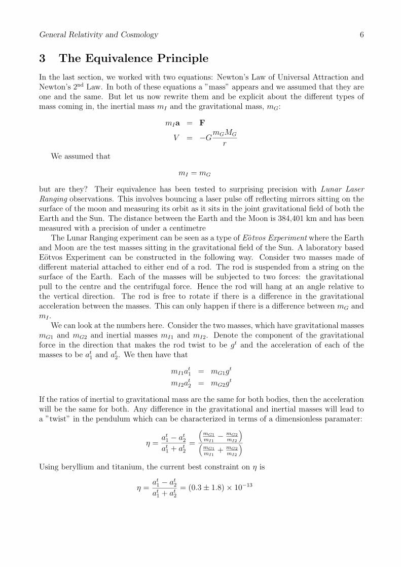
The Lunar Ranging experiment can be seen as a type of Eotvos Experiment where the Earthand Moon are the test masses sitting in the gravitational field of the Sun. A laboratory basedEotvos Experiment can be constructed in the following way. Consider two masses made ofdifferent material attached to either end of a rod. The rod is suspended from a string on thesurface of the Earth. Each of the masses will be subjected to two forces: the gravitationalpull to the centre and the centrifugal force. Hence the rod will hang at an angle relative tothe vertical direction. The rod is free to rotate if there is a difference in the gravitationalacceleration between the masses. This can only happen if there is a difference between mG andmI .
We can look at the numbers here. Consider the two masses, which have gravitational massesmG1 and mG2 and inertial masses mI1 and mI2. Denote the component of the gravitationalforce in the direction that makes the rod twist to be gt and the acceleration of each of themasses to be at1 and at2. We then have that
mI1at1 = mG1g
t
mI2at2 = mG2g
t
If the ratios of inertial to gravitational mass are the same for both bodies, then the accelerationwill be the same for both. Any difference in the gravitational and inertial masses will lead toa ”twist” in the pendulum which can be characterized in terms of a dimensionless paramater:
η =at1 − at2at1 + at2
=
(
mG1
mI1− mG2
mI2
)
(
mG1
mI1+ mG2
mI2
)
Using beryllium and titanium, the current best constraint on η is
η =at1 − at2at1 + at2
= (0.3± 1.8)× 10−13
General Relativity and Cosmology 7
Twisting
direction
Fiber
Earth’s
rotation
! T
m
I
! a
mG
! g
Figure 1: The pendulum for the Eotvos Experiment
which is a factor of 4 better than the original Eotvos experiment of 1922. To date, one of themost successful tests is to use the Earth-Moon system in the gravitational field of the Sun as agiant Eotvos experiment. The difference, with regards to the lab based Eotvos experiments, isthat the masses of the test bodies (i.e. the Earth and Moon) are not negligible any more. Thetest can be done by using lasers reflected off mirrors left on the Moon by the Apollo 11 missionin 1969 and, as mentioned earlier, the constraint is
η = (−1.0± 1.4)× 10−13
This is one of the most accurately tested principles of physics and we expect this constraint toimprove by 5 orders of magnitude when space based tests can be performed.
If the gravitational and inertial masses are the same, then we have that a particle in agravitational field will obey
r =mG
mI
g = g
and this will be true of any particle. This has a profound consequence-it means that I canalways find a time dependent coordinate transformation (from r to R),
r = R+ b(t)
such that
R = g − b(t) = 0
In other words, it is always possible to pick an accelerated reference frame such that the observerdoesn’t feel the gravitational field at all. For example, consider a particle at rest near the surfaceof the Earth. It will feel a gravitational pull of g = −9.8ms−2. Now place it in a referenceframe such that b = 1
2gt2 (such as a freely falling elevator). Then the particle at rest in this
reference frame won’t feel the gravitational pull.
General Relativity and Cosmology 8
A
B
t = 0
first pulse
emitted by A
t = t1
first pulse
received by B
A
B
A
B
t = !"A
second pulse
emitted by A
t = t1+!"B
second pulse
received by B
A
B
z
t
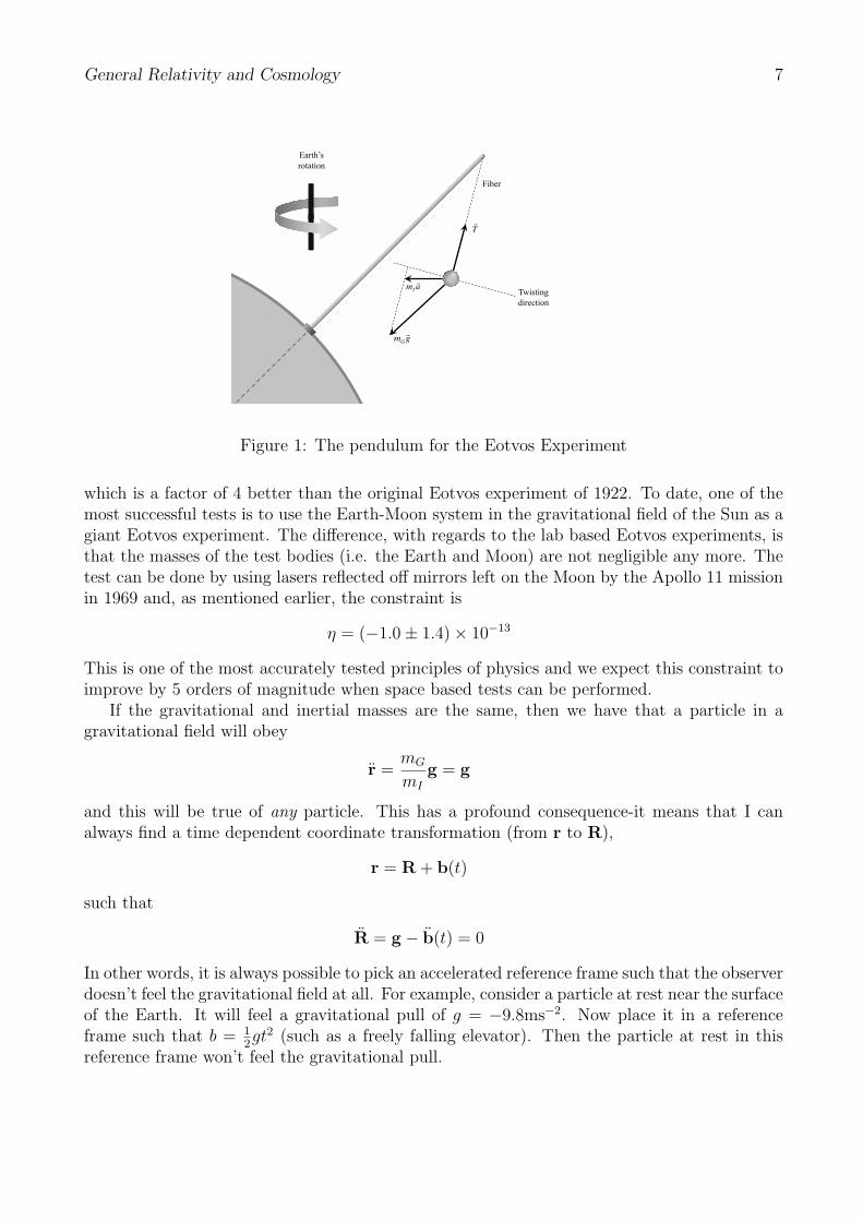
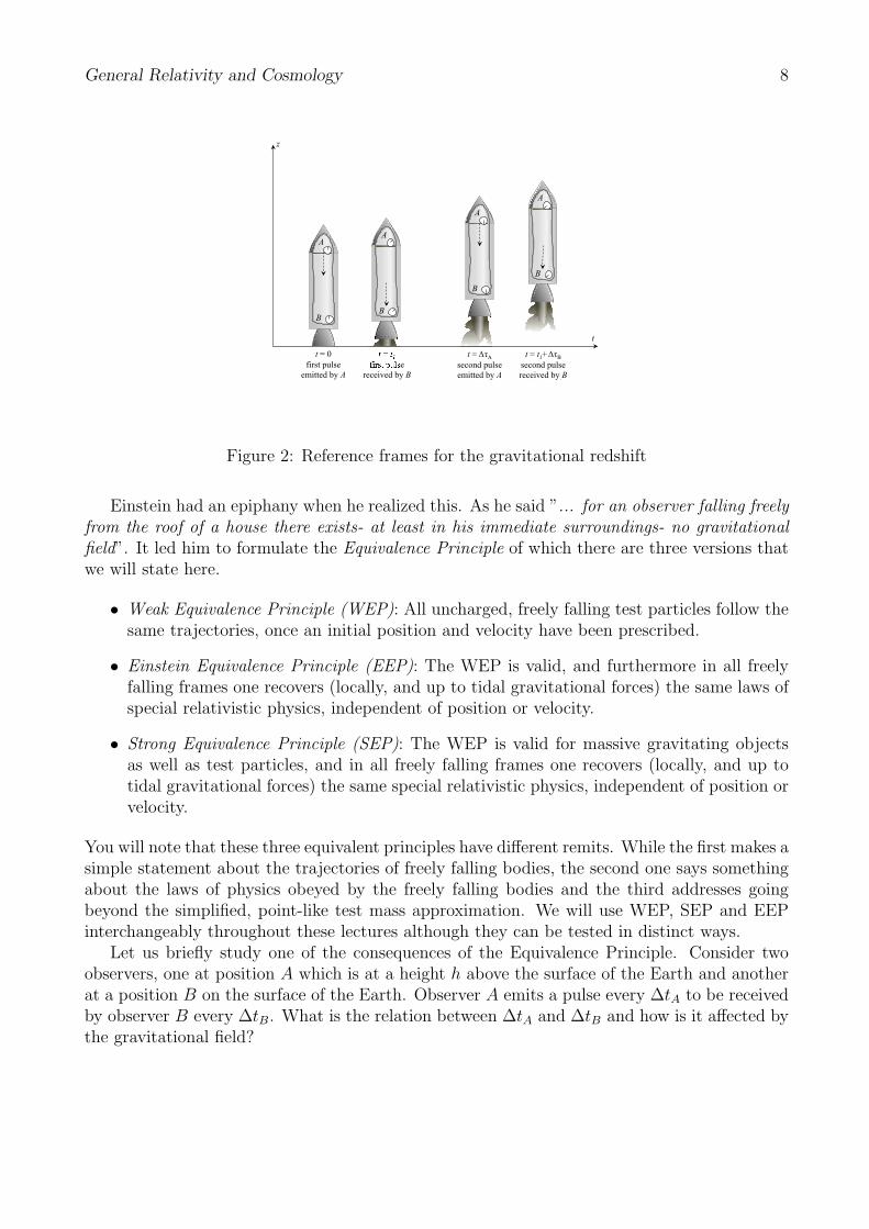
Figure 2: Reference frames for the gravitational redshift
Einstein had an epiphany when he realized this. As he said ”... for an observer falling freelyfrom the roof of a house there exists- at least in his immediate surroundings- no gravitationalfield”. It led him to formulate the Equivalence Principle of which there are three versions thatwe will state here.
• Weak Equivalence Principle (WEP): All uncharged, freely falling test particles follow thesame trajectories, once an initial position and velocity have been prescribed.
• Einstein Equivalence Principle (EEP): The WEP is valid, and furthermore in all freelyfalling frames one recovers (locally, and up to tidal gravitational forces) the same laws ofspecial relativistic physics, independent of position or velocity.
• Strong Equivalence Principle (SEP): The WEP is valid for massive gravitating objectsas well as test particles, and in all freely falling frames one recovers (locally, and up totidal gravitational forces) the same special relativistic physics, independent of position orvelocity.
You will note that these three equivalent principles have different remits. While the first makes asimple statement about the trajectories of freely falling bodies, the second one says somethingabout the laws of physics obeyed by the freely falling bodies and the third addresses goingbeyond the simplified, point-like test mass approximation. We will use WEP, SEP and EEPinterchangeably throughout these lectures although they can be tested in distinct ways.
Let us briefly study one of the consequences of the Equivalence Principle. Consider twoobservers, one at position A which is at a height h above the surface of the Earth and anotherat a position B on the surface of the Earth. Observer A emits a pulse every ∆tA to be receivedby observer B every ∆tB. What is the relation between ∆tA and ∆tB and how is it affected bythe gravitational field?
General Relativity and Cosmology 9
Given what we have seen above, we can think of this as two observers moving upwards withan acceleration g. We have that the positions of A and B are given by
zA(t) =1
2gt2 + h
zB(t) =1
2gt2
Now assume the first pulse is emitted at t = 0 by A and is received at time t1 by B. Asubsequent pulse is then emitted at time ∆tA by A and then received at time t1 + ∆tB. Wehave that
zA(0)− zB(t1) = h− 1
2gt21 = ct1
zA(∆tA)− zB(t1 +∆tB) = h+1
2g∆t2A − 1
2g(t1 +∆tB)
2
≃ h− 1
2gt21 − gt1∆tB = c(t1 +∆tB −∆tA)
where we have discarded higher order terms in ∆t. Combining the two equations, and assumingt1 ≃ h/c we have that
∆tA ≃ (1 +gh
c2)∆tB
In other words, there is gravitational time dilation due to the difference in the gravitationalpotentials at the two points ΦB − ΦA = −gh so
Rate Received =(
1− ΦB − ΦA
c2
)
× Rate Emitted
This is known as the gravitational redshift of light.
4 Geodesics
In the previous section, we saw how important accelerated reference frames could be. From thevarious equivalence principles, it seems that an accelerating reference frame will be indistin-guishable from a frame in a gravitational field. Let us then study how particles and observerstravel through space.
In flat space, a particle follows straight lines given by solutions to the kinematic equationsof motion
d2xα
dτ 2= 0
The particle will trace out a path in space-time xα(τ) and the solution is of the form
xα(τ) = xα(τi) + uα(τ − τi)
where xα(τi) and uα are integration constants.
General Relativity and Cosmology 10
In the presence of a gravitational field, the path taken by a particle will be curved. Alterna-tively, in an accelerating reference frame, the same will happen. We call Geodesics the shortestpaths between two points in space-time. We have just written down the geodesic in a flat, forcefree space. If we wish to do so in the presence of a gravitational field, we need to solve theGeodesic equation. As Einstein argued, according to the principle of equivalence, there shouldbe a freely falling coordinate system yα in which particles move in a straight line and thereforesatisfy
d2yα
dτ 2= 0
where τ is the proper time of the particle and hence
c2dτ 2 = −ηαβdyαdyβ
Now choose a different coordinate system, xµ; it can be at rest, accelerating, rotating, etc. Wecan reexpress the yαs in terms of the xµ, yα(xµ). Using the chain rule we have
0 =d
dτ
(
∂yα
∂xµ
dxµ
dτ
)
=∂yα
∂xµ
d2xµ
dτ 2+
∂2yα
∂xµ∂xν
dxµ
dτ
dxν
dτ
Multiplying through by the inverse Jacobian ∂xβ/∂yα we end up with the geodesic equationwith the form
d2xβ
dτ 2+ Γβ
µν
dxµ
dτ
dxν
dτ= 0 (4)
where we have defined the affine connection
Γβµν =
∂xβ
∂yα∂2yα
∂xµ∂xν
We can also express the proper time in these new (or arbitrary coordinates) as
c2dτ 2 = −ηαβ∂yα
∂xµdxµ∂y
β
∂xνdxν ≡ −gµνdx
µdxν
where we have defined the metric:
gµν = ηαβ∂yα
∂xµ
∂yβ
∂xν
The situation is slightly different for a massless particle. Neutrinos or photons follow nullpaths so dτ = 0. Instead of using τ we can use some other parameter σ. We then have
d2yα
dσ2= 0
−ηαβdyα
dσ
dyβ
dσ= 0
General Relativity and Cosmology 11
ne One can repeat the same derivation as above to find
d2xµ
dσ2+ Γµ
αβ
dxα
dσ
dxβ
dσ= 0
−gαβdyα
dσ
dyβ
dσ= 0
So, given an Γµαβ and gαβ, we can work out the equations in a given reference frame.
It turns out that we can simplify the calculation even further: Γµαβ can be found from gαβ.
Taking the partial derivative of the metric, we have that
∂gµν∂xλ
=∂2yα
∂xλ∂xµ
∂yβ
∂xνηαβ +
∂2yβ
∂xλ∂xν
∂yα
∂xµηαβ
From the definitiion of Γµαβ we can replace it in the above expression
∂gµν∂xλ
= Γγλµ
∂yα
∂xγ
∂yβ
∂xνηαβ + Γγ
λν
∂yβ
∂xγ
∂yα
∂xµηαβ
which can be written as
∂gµν∂xλ
= Γγλµgγν + Γγ
λνgγµ
We can now permute indices and add them to solve and find
Γµαβ =
1
2gµν
(
∂gαν∂xβ
+∂gνβ∂xα
− ∂gαβ∂xν
)
Hence, as advertised, given a metric, gµν , we can find the connection coefficents Γµαβ and then
solve the geodesic equation.It often useful to find the geodesic equations in terms of a variational principle. In fact, it is
also a convenient method for, given a metric, calculating the connection coefficients. Considera path in space time xα(λ). We can define the proper time elapsed between two points on thatcurve, A and B, to be
cτAB =∫ B
ALdλ =
∫ B
Adλ√
−ηαβxαxβ
The derivatives are taken with regards to λ. It is now possible to define an action for the pathxα(λ):
S = −mc2τ
and we can minimize this action to find the path which takes the most amount of proper timebetween points A and B. This path will be the geodesic. For example, if we choose x0 = cλ = ctwe have that
S = −mc∫
dt
√
√
√
√c2 −(
dx
dt
)2
General Relativity and Cosmology 12
More generally, we can use the Euler Lagrange equations:
d
dλ
(
∂L
∂xα
)
=∂L
∂xα
Given that L is independent of xα (and dτ = Ldλ) we have that the equation of motion becomes
∂L
∂xα= −1
2
1
Lηαβ
dxβ
dλ= −1
2ηαβ
dxβ
dτ
The resulting equations then become
d2xα
dτ 2= 0
Although the above action is reparametrization invariant (i.e. we can change our definition ofλ and the action is unaffected), the square root is difficult to work with. It is easier to workwith
S = −m∫
dληαβdxα
dλ
dxβ
dλ= m
∫
dλL2
The Euler-Lagrange equation then becomes
∂L2
∂xµ− d
dλ
(
∂L2
∂xµ
)
= −2dL
dλ
∂L
∂xµ
Again, if we choose the affine parameter λ to be linear in τ we have that the right hand sidebecomes
dL
dλ=
d
dλ
(
cdτ
dλ
)
= 0
So, for a massive particle it makes sense to choose λ = τ . Finally we, can rederive the geodesicequation from the action principle as above, but in the presence of a gravitational field. Wenow have
S = m∫
dλgµνdxµ
dλ
dxν
dλ= m
∫
dλL2
and can apply the Euler-Lagrange equation to obtain the Geodesic equation in a general frame.
5 Coordinate Transformations and Metrics
We have seen that coordinate transformations to accelerated reference frames lead to non-trivial geodesic equations. We have considered one such transformation when deriving thegravitational redshift. Let us now look at coordinate transformations in more detail.
You have extensively studied coordinate transformations between inertial reference frames(in the absence of gravitational fields) in Special Relativity. For example, consider a coordinate
General Relativity and Cosmology 13
transformation along the z-axis from a stationary frame to one moving at a velocity v. Wehave that the coordinate transformation can be expressed in a matrix form as
x0
x1
x2
x3
=
γ 0 0 −βγ0 1 0 00 0 1 0
−βγ 0 0 γ
x0
x1
x2
x3
where β = v/c and γ = 1/√1− β2. This coordinate transformation is of the form
xµ = xµ(xν)
and given that it is linear, we have that the Jacobian is simply:
∂xµ
∂xν=
γ 0 0 −βγ0 1 0 00 0 1 0
−βγ 0 0 γ
Now, in special relativity we have that the space time interval
ds2 = −c2dt2 + (dx1)2 + (dx2)2 + (dx3)2
is invariant under coordinate transformations. We can restate this as
ds2 = ηαβdxαdxβ = ηαβdx
αdxβ
in other words, the transformation leaves the actual form of the space time interval invariant.What happens if we now consider a coordinate transformation to an accelerating refer-
ence frame? Let us consider the simplest case, an accelerating reference frame, with accelera-tion g, along the x3 direction. We have that the transformation between the old coordinates,(x0, x1, x2, x3) and the new coordinates, (x0, x1, x2, x3), is given by
x0 =c2
ge
gx3
c2 sinh(g
c2x0)
x1 = x1
x2 = x2
x3 =c2
ge
gx3
c2 cosh(g
c2x0)
We can transform the expression for the space-time interval to the new coordinate system:
ds2 = ηαβdxαdxβ = −(dx0)2 + (dx1)2 + (dx2)2 + (dx3)2
= −e2gx3
c2 (dx0)2 + (dx1)2 + (dx2)2 + e2gx3
c2 (dx3)2
Note that the equivalent gravitational potential has the form Φ = gx3 and so the interval takesthe form
ds2 = −e2Φ
c2 (dx0)2 + (dx1)2 + (dx2)2 + e2Φ
c2 (dx3)2 (5)
General Relativity and Cosmology 14
In fact, this expression is valid in a more general setting than just a constant gravitationalacceleration. A weak, static gravitational field, Φ is equivalent to a metric of this form.
For the remainder of this section let us familiarize ourselves a bit more with coordinatetransformations and how they affect the metric. With a general coordinate transformation,xα = xα(xβ) we find that the space time interval changes as
ds2 = ηαβdxαdxβ = ηαβ
∂xα
∂xµ
∂xβ
∂xνdxµdxν ≡ gµνdx
µdxν
In other words, under a general coordinate transformation, we have that ηµν → gµν . We callthe object gµν the metric.
The metric contains information about the geometry of space (and space-time) we areconsidering. It is instructive to work through a few examples. For example, consider a 2-Dsheet plane, with coordinates (x, y). The interval on that plane is given by
ds2 = dx2 + dy2
and hence the metric is very simple: it is a diagonal matrix with entries
gij =
(
1 00 1
)
We can transform to polar coordinates
x = r cos θ
y = r sin θ
to find
ds2 = dr2 + r2dθ2
Note that now the metric is more complicated:
gij =
(
1 00 r2
)
yet it still describes a plane. We could have considered a different surface, a sphere with unitradius. It is a two dimensional surface and hence needs two coordinates, (θ, φ). The infinitesimalinterval is defined as
ds2 = dθ2 + sin2(θ)dφ2
with metric
gij =
(
1 00 sin2(θ)
)
The geometry of the surface of a sphere is obviously very different to the geometry of a planeand it is in the metric that this information is encoded.
General Relativity and Cosmology 15
We are of course, interested in the geometry of 3-D space and of 4-D space time. So, forexample, the interval (and metric) for Euclidean (or flat) 3-D space in Cartesian coordinatesare
ds2 = (dx1)2 + (dx2)2 + (dx3)2
and
gij =
1 0 00 1 00 0 1
In spherical coordinates
x1 = r sin(θ) cos(φ)
x2 = r sin(θ) sin(φ)
x3 = r cos(θ)
we have that the interval (and metric) are
ds2 = dr2 + r2dθ2 + r2 sin2(θ)dφ2
and
gij =
1 0 00 r2 00 0 r2 sin2(θ)
Again, these two metrics (in Cartesian and spherical coordinates) describe exactly the samespace.
We have already seen examples of space-time metrics above. The Minkowski metric andthe metric of an accelerated observer (known as a Rindler metric).
Let us now consider two important metric. The first one is that of a Euclidean, homogeneousand isotropic spacetime. We have that
ds2 = −c2dt2 + a2(t)[
(dx1)2 + (dx2)2 + (dx3)2]
(6)
which has a metric
gµν =
−1 0 0 00 a2(t) 0 00 0 a2(t) 00 0 0 a2(t)
A particularly important metric is a static (i.e. time independent), spherically symmetricSchwarzschild metric:
ds2 = −(
1− 2GM
c2r
)
c2dt2 +(
1− 2GM
c2r
)−1
dr2 + r2dθ2 + r2 sin2(θ)dφ2 (7)
General Relativity and Cosmology 16
which has a metric
gµν =
−(
1− 2GMc2r
)
0 0 0
0(
1− 2GMc2r
)−10 0
0 0 r2 00 0 0 r2 sin2(θ)
This metric is of particular importance. It corresponds to the space time of a point like massand can be used to describe the space time around stars, planets and black holes.
To finish, let us calculate the geodesics for the homogeneous metric to find out what theconnection coefficients are. The action is:
L2 = −c2t2 + a2(t)∑
(xi)2
where f = dfdλ. The Euler-Lagrange equations are:
x0 +a
c
da
dt
∑
(xi)2 = 0
xi + 21
ac
da
dtx0xi = 0
We can now read off the connection coefficients (and be careful not to over count with thefactor of 2 in the second expression):
Γ0ij =
1
cada
dtδij
Γi0j =
1
ac
da
dtδij
6 The Newtonian Limit and the Gravitational Redshift
Revisited
Interestingly enough, with what we have done we can already start relating the geodesic equa-tion with the Newtonian regime of gravity. Let us look at the case where the gravitational fieldis extremely weak and stationary and particles are moving at non-relativistic speeds so v ≪ c.Let us start with the geodesic equation:
d2xµ
dτ 2+ Γµ
αβ
dxα
dτ
dxβ
dτ= 0
The non-relativistic approximation means that dxi/dτ ≪ d(ct)/dτ so the geodesic equationsimplifies to
d2xµ
dτ 2+ Γµ
00
(
dx0
dτ
)2
≃ 0
If the gravitational field is stationary we have that ∂gµν/∂t = 0 and we have
Γµ00 = −1
2gµλ
∂g00∂xλ
General Relativity and Cosmology 17
Now consider a weak field
gµν = ηµν + hµν
where we assume that |hµν | ≪ 1. We can expand Γµ00 to first order in hµν to find
Γµ00 = −1
2ηµν
∂h00
∂xν
Only the spatial parts of ηµν survive (which are 1). Hence we have
Γµ00 = −1
2
∂h00
∂xµ
The geodesic equation then becomes
d2xµ
dτ 2=
1
2
(
dx0
dτ
)2∂h00
∂xν
which in vectorial notation becomes
d2r
dτ 2=
1
2
(
dx0
dτ
)2
∇h00
For small speeds dt/dτ ≃ 1 and comparing with the Newtonian result d2rdt2
= −∇Φ we see that
h00 = −2Φ
c2
Hence in the weak-field limit
g00 = −(
1 +2Φ
c2
)
Note that, if we take the metric that we found in equation 5 and expand to linear order (i.e.take the weak field limit), we get exactly the same expression.
We can rederive our expression for the gravitational redshift directly from the metric. Con-sider the proper time again
−ds2 = c2dτ 2 = −gµνdxµdxν
and pick a stationary system so dxi = 0. We then have
dτ =√−g00dt.
In the weak field case we have
dτ ≃(
1 +Φ
c2
)
dt
General Relativity and Cosmology 18
Note that t and τ only coincide if Φ = 0 so clocks run slowly in potential wells. We can nowcompare the rate of change at two points, A and B, to get
dτAdτB
=
√
√
√
√
g00(A)
g00(B)
which in the weak field limit gives the ratio of frequencies
νBνA
=dτAdτB
≃ 1− ΦB − ΦA
c2
which is equivalent to the expression we found in Section 3. We can define the gravitationalredshift
zgrav ≡νA − νB
νA=
ΦB − ΦA
c2
This is a very small effect- for the Sun it is ∼ 10−6.One way to look for this effect is by studying the spectral lines emitted from atoms which
are very close to a massive body and hence deep into a gravitational potential. This effecthas been observed in the Sun and white dwarfs but these observations are not very accurate.A classic test of the gravitational redshift was undertaken by Pound and Rebka in 1960 atHarvard. They used a 22.5 metre high tower where they placed an unstable nucleus, Fe57
at the top and the bottom. The nucleus (at the top) would emit gamma-rays with a certainfrequency related to their energy. These rays would fall to the bottom and interact with theFe57 there. If the gamma rays of the observer were the same as the emitter, the Fe57 at thebottom of the shaft would react. But because of the gravitational redshift, the frequency wasshifted and the absorption was less efficient. By changing the velocity of the source at the topof the tower, the experimenters could compensate for the gravitational effect and measure it towithin 1%.
Better measurements of the gravitational redshifting of light can be obtained on (or near) theEarth where, even though the gravitational field is much, much weaker, there is the possibilityto make very precise measurements. One way to do this is to send a rocket up into orbit witha hydrogen-maser clock and emitting pulses to a ground station. At an altitude of 104 Km, thechange in gravitational potential will be gh/c2 ≃ 10−10. Note that this effect is minute, almost5 orders of magnitude smaller than the simple Doppler effect due to the motion of the rocket.Yet it is still possible to constrain the effect to within 0.002%.
7 Orbits I: the Perihelion of Mercury
It is now time to revisit the two body problem. We have already worked this out for theNewtonian case but we can now see what happens if we consider the more general case. Strictlyspeaking we will be studying the motion of mass µ in a central potential sourced by a mass M .
We can use the Schwarzschild metric that we introduced in equation 7 of the previoussection. The total mass is M and the reduced mass is µ. The action for the geodesic equationfor (t(λ), r(λ), θ(λ), φ(λ)) in this metric is
L2 =(
1− 2GM
rc2
)
c2t2 − r2
1− 2GMrc2
− r2(θ2 + sin2 θφ2)
General Relativity and Cosmology 19
The angular Euler-Lagrange equations are exactly as in the Newtonian two body problem wepreviously solved
d
dλ(2r2θ) = 2r2 sin θ cos θφ2
d
dλ(2r2 sin2 θφ) = 0
and we can solve them in the same way, placing the orbit on the equatorial plane, choosingintegration constants such that θ = 0 so that
r2φ =J
µ
The timelike component of the geodesic obeys
d
dλ
[
c2(
1− 2GM
rc2
)
t]
= 0
which can be integrated to give(
1− 2GM
rc2
)
t = k
For a massive particle we have L2 = c2
c2 =c2k2 − r2(
1− 2GMc2r
) − J2
µ2r2
which can be rewritten
r2 +(
1− 2GM
c2r
)
J2
µ2r2= c2k2 − c2 +
2GM
r
Rearranging we find
r2 +J2
µ2r2− 2GM
r− 2GMJ2
µ2r3c2= constant (8)
We can compare this expression with the one we found in the Newtonian case in equation 2:
r2 +h2
r2− 2GM
r= constant
There is an extra term in the General Relativistic case. Furthermore, in the Newtonian casewe are taking derivatives with regards to t while in the General Relativistic case we are usingthe affine parameter λ.
We would now like to find the orbits of motion in this system. As in the Newtonian case,using conservation of angular momentum we can change the independent variable from λ to φ.Furthermore, we can transform to u = 1/r so that
r =dr
dφ
dφ
dλ= − 1
u2
du
dφ
J
µu2 = −J
µ
du
dφ
General Relativity and Cosmology 20
Dividing through by J2/µ2, equation 8 becomes(
du
dφ
)2
+ u2 − 2GMµ2
J2u− 2GM
c2u3 = constant
Differentiating by φ and dividing by 2dudφ
we find
d2u
dφ2+ u =
Gmµ2
J2+
3GM
c2u2
You will see that this equation has a very similar form to equation 3 with an extra bit. It isuseful to rescale u so as to assess how important the correction is. Define U = J2
GMµ2u. We thenhave
d2U
dφ2+ U = 1 + ǫU2 (9)
with ǫ ≡ 3G2M2µ2/J2c2. We will see that ǫ in the case of Mercury, is of order 10−7, so verysmall. We therefore assume that U can be split into a Newtonian part, U0 and a small, generalrelativistic correction, U1. We have that U0 = 1 + e cos(φ) which we can plug into equation 9to find (to lowest order):
d2U1
dφ2+ U1 = ǫU2
0 = ǫ[1 + 2e cos(φ) + e2 cos2(φ)] = ǫ[1 +e2
2+ 2e cos(φ) +
e2
2cos(2φ)]
The complementary function is as before but the particular integral takes the form
U1 = ǫ
[(
1 +e2
2
)
+ eφ sin(φ)− e2
6cos(2φ)
]
With time, the dominant term will be proportional to φ so that, adding the complementaryfunction and the particular integral we have
U ≃ 1 + e cos(φ) + ǫeφ sin(φ)
This corresponds to the Taylor expansion of
U ≃ 1 + e cos[φ(1− ǫ)]
I.e. the period of the orbit is now 2π/(1− ǫ) and not 2π. The orbit does not close in on itself.We can work out what this correction is for Mercury. Taking M ≃ 2 × 1030 kg, the orbitalperiod T = 88 days and the mean orbital radius r = 5.8 × 10¹⁰ m, we find ǫ ≃ 10−7 so thatprecession rate is approximately 43 arc seconds per century. This effect, first detected by LeVerrier in the mid 19th century is obscured by a number of other effects. The precession of theequinoxes of the coordinate systems contributes to about 5025” per century while the otherplanets contribute about 531” per century. The Sun also has a quadropole moment whichcontributes a further 0.025” per century. Taking all these effects into account still leaves aprecession of θ for which the current best estimate is
θ = 42.969”± 0.0052” per century
The prediction from General Relativity is
θ ≃ 42.98” per century
General Relativity and Cosmology 21
8 Orbits II: Gravitational Lensing and the Shapiro Time
Delay
We now want to study what happens to a light ray propagating in a gravitational field. We firstwork out what happens in a Newtonian universe; we are going to model a photon as a massiveparticle travelling at the speed of light, c with angular momentum per unit mass h = cR. Recallthat u = 1/r satisfies
d2u
dφ2+ u =
GM
h2=
GM
c2R2
We have solved it before for closed orbits but we now want to pick integration constants thatlead to unbounded orbits:
u =sinφ
R+
GM
c2R2
where R is the distance of closest approach in the absence of gravity. Consider the asymptoticbehaviour: when r → ∞ we have u → 0 which gives us two solutions for φ: φ− = −GM/(c2R)and φ+ = π +GM/(c2R). The total deflection is
∆φN =2GM
c2R
We can now repeat the calculation for in the relativistic case. As in Section 7, we have thatthe geodesic equation for a light ray must be parametrized in terms of an affine parameter andnot proper time. We can use some of the results found in 7 (and, once again, taking θ = π/2)
r2φ = h(
1− 2GM
rc2
)
t = k
For a massless particle we have L2 = 0
0 =(
1− 2GM
c2r
)
c2t2 − r2(
1− 2GMc2r
) − h2
r2
which can be rewritten in terms of u as
h2
(
du
dφ
)2
= c2k2 − h2u2 +2GM
c2h2u3
which, when differentiated gives
d2u
dφ2+ u =
3GM
c2u2
Again, we can treat the right hand side as a small perturbation to the orbit
u0 =sinφ
R(10)
General Relativity and Cosmology 22
This equation corresponds to a straight line. The first order equation is
d2u1
dφ2+ u1 =
3GM
c2R2sin2 φ =
3GM
2c2R2(1− cos 2φ)
which combined with u0 leads to the complete, first order, solution
u =sinφ
R+
3GM
2c2R2
(
1 +1
3cos 2φ
)
At large distances, u → 0 and assuming sinφ ≃ φ we have two possible solutions for φ:φ− = −2GM
c2Rand φ+ = π + 2GM
c2R. The total deflection is then
∆φGR =4GM
c2R
We find that ∆φGR = 2∆φN .For a light ray grazing the limb of the Sun, the deflection will be θ ≃ 1.75”, famously
measured by Arthur Eddington during his Eclipse expedition in 1919. The tightest observa-tional constraint come from observations due to Shapiro, David, Lebach and Gregory who usedaround 2500 days worth of observation taken over 20 years- they used 87 VLBI sites and 541radio sources yielding more than 1.7× 10⁶ observations and and obtained a constraint on θ:
θ = (0.99992± 0.00023)× 1.75′′
which is 3 orders of magnitude better than Eddington’s original observations.Another relativistic effect involving light rays is the Shapiro time delay, first proposed in
1964. Again, take the Schwarzschild metric in the equatorial plane and apply to electromagneticwave (radar) propagating at the speed of light. We have that ds2 = 0 so
0 =(
1− 2GM
c2r
)
c2dt2 − dr2(
1− 2GMc2r
) − r2dφ2
Take the unperturbed solution, given in equation 10. We have
−dr
r2=
cos(φ)
Rdφ
which can be used to find
r2dφ2 = dr2 tan2 φ =R2dr2
r2 −R2
The metric can then be rewritten as
c2dt2 = dr2[
(
1− 2GM
c2r
)−2
+(
1− 2GM
c2r
)−1 R2
r2 −R2
]
We can now expand to first order in GM/(rc2) to find
cdt = ± rdr√r2 −R2
[
1 +2GM
rc2− GMR2
r3c2
]
General Relativity and Cosmology 23
This expression can be easily integrate between points A and B to give
c∆t = ±
√r2 −R2 +
2GM
c2ln
√
r2
R2− 1 +
r
R
− GM
c2
√
1− R2
r2
B
A
(11)
We can now apply this to a planetary system. Let us take A to be the Earth and B to beVenus. The expression in equation 11 for ∆t is the coordinate elapsed, not the time elapsed onthe Earth, ∆τ . To relate these two time intervals recall that
ds2 = −c2dτ 2
where dτ is the proper time elapsed at on the Earth. We can assume a circular orbit so thatdr = dθ = 0 but clearly we have dφ 6= 0. We are then left with
c2dτ 2 =(
1− 2GM
c2rE
)
c2dt2 − r2dφ2
where rE is the Earth-Sun distance. We can simplify to
dτ =
√
√
√
√1− 2GM
c2rE− r2
c2
(
dφ
dt
)2
dt
On a circular orbit we can use Kepler’s law
(
dφ
dt
)2
=GM
r3
so we find
∆τ =
√
1− 2GM
c2rE− GM
c2rE∆t =
√
1− 3GM
c2rE∆t ≃
(
1− 3GM
2c2rE
)
∆t
To understand what one should expect, take r ≫ R and look at the expression to see whichterm dominates as R → 0. The logarithmic term will diverge so that, when a light ray passesclose to the source, there is a large time delay. So, by monitoring a regular pulse of light asit passes behind a massive body, one should see a large include in the period, a characteristicspike during the transit. Shapiro proposed an experiment where one would send light rays(or radar signals) from the Earth which would then be reflected off Venus and back. If theEarth and Venus are aligned, the Sun induces an effect on the order of microseconds. In fact,when receiving signals from distant satellites such Voyager and Pioneer, one has to include theShapiro time delay effect in processing their signals. The best constraints are due to Bertotti,Iess and Tortora using radio links with Cassini in 2002 which give us
t = (1.00001± 0.00001)tGR
where tGR is the prediction from General Relativity.
General Relativity and Cosmology 24
9 The Equivalence Principle and General Covariance
The Equivalence Principle has led us to move away from preferred frames or even preferredcoordinate systems. A modern theory of gravity must take that into account, i.e. it should bepossible to write the laws of physics in a form which is true in any coordinate system. This isknown as the Principle of General Covariance.
To implement General Covariance we have to learn a little bit more about geometry. For astart let us recall how we transform between different coordinate systems. Consider a coordinatetransformation xµ = xµ(xν). The Jacobian matrix of the transformation is defined to be
∂xµ
∂xν
Given another coordinate transformation xµ = xµ(xν), we can apply the chain rule to get:
∂xµ
∂xν=
∂xµ
∂xα
∂xα
∂xν
and
∂xµ
∂xα
∂xα
∂xν= δµν
How do different types of functions of xµ transform under coordinate transformations. Thesimplest case is a scalar field, φ(xµ)- it remains unchanged under a coordinate transformation.A simple example of a scalar is dτ , which we used in Section 4 to construct the invariant actionfor the geodesic.
The next type of functions are vectors fields. Consider a curve in space time, parametrizedby λ so xα = xα(λ). The tangent vector field is given by
T α =dxα
dλ
Suppose we now change coordinates to xα. We now have that the tangent vector in these newcoordinates is
T α =dxα
dλ. (12)
Using the chain rule we have
dxα
dλ=
∂xα
∂xβ
dxβ
dλ
So the tangent vector field transforms as
T α =∂xα
∂xβT β
A vector field with the indices ”up” (and which therefore transforms in this way) is known asa contravariant vector field.
General Relativity and Cosmology 25
There is a different type of vector field, with an index ”down” which is known as a covariantvector field. An example is
Fα =∂f
∂xα
i.e. the gradient of a function f(x). The chain rule gives
∂f
∂xα=
∂xβ
∂xα
∂f
∂xβ
So definining
Fα =∂f
∂xα
we have
Fα =∂xβ
∂xαFβ
Note how the transformation matrix is the inverse of the one for contravariant tensors. Thisof course, means that if you contract something with an ”up” index with something with a”down” index you have
T αFα =∂xα
∂xβ
∂xγ
∂xαT βFγ = δγβT
βFγ = T βFβ
i.e. the resulting object is a scalar and unchanged by a coordinate transformation.It should be obvious that we can generalize this to objects with arbitrary number of ”up”
and ”down” indices. These objects are known as tensors. We have already had to deal withone of them, the metric. The metric is a 2nd rank tensor and transforms as
gαβ =∂xµ
∂xα
∂xν
∂xβgµν
We can also define the inverse of the metric which is simply the contravariant version of themetric, gαβ and satisfies:
gαµgµβ = δαβ
We can generalize to an arbitrary tensor. For example a 2nd rank contravariant tensor willbe represented as Mαβ, a 2nd rank covariant tensor will be of the form Nαβ and a 2nd rankmixed tensor will have the form Oα
β. We can have higher order tensors (and we will comeacross one later on). For example a 4th order mixed rank tensor will be of the form Rα
βµν .We have now constructed this array of objects and wish to do operations on them. The
most important operation we need to do is differentiation. Let us see why we can’t use normalderivatives. We’ve already seen that Fα = ∂f
∂xα transforms in the correct way. Let us nowconsider the 2nd derivative of Fα:
∂Fα
∂xβ
General Relativity and Cosmology 26
Again let us consider a change of coordinates:
∂Fα
∂xβ=
∂2f
∂xα∂xβ=
∂xγ
∂xα
∂
∂xγ
(
∂xδ
∂xβ
∂f
∂xδ
)
=∂xγ
∂xα
∂xδ
∂xβ
∂2f
∂xγ∂xδ+
∂2xδ
∂xα∂xβ
∂f
∂xδ
If we were working with a covariant tensor we wouldn’t have the extra term. So the normal,2nd derivative of a scalar (i.e. the Hessian) is not a 2nd covariant tensor.
We can define the covariant derivative, ∇α which obeys the following properties
• ∇αf = ∂f∂xα
• It obeys the Liebnitz rule
∇α(MN) = (∇αM)N +M(∇αN)
for any two tensors M and N (we have hidden the indices).
• ∇α commutes with contractions between indices.
We can construct such an operator as follows. It is a normal derivative when applied to ascalar. Applied to contravariant or covariant vector fields it acts as
∇αVβ = ∂αV
β + ΓβαµV
µ
∇αUβ = ∂αUβ − ΓµαβUµ
The objects that we have denoted by Γµαβ are exactly the connection coefficients that we came
across when constructing the geodesic equations. We can use them to construct the covariantderivatives of 2nd rank tensors too. So, for example we have
∇αMµν = ∂αMµν − ΓβαµMβν − Γβ
ανMµβ
∇αNµν = ∂αN
µν + ΓµαβN
βν + ΓναβN
µβ
∇αOµν = ∂αO
µν + Γµ
αβOβν − Γβ
ανOµβ
Finally, the covariant derivative constructed in this way satisfies the metricity condition:
∇αgµν = 0
Now let us revisit our curve on space-time xα = xα(λ). We can define the absolute derivativeof a vector V µ along that path to be
DV µ
Dλ≡ T α∇αV
µ
where the tangent vector T α is defined in equation 12. We say that the vector V µ is parallelytransported along that path if
DV µ
Dλ= 0
General Relativity and Cosmology 27
This is a differential equation for V µ. We can start at a point xα(λ = 0) and integrate to findthe value V µ at, for example, the point xα(λ = 1). The result is path dependent. The paralleltransport equation applied to T α is
DT α
Dλ= 0
can be rewritten as
d2xα
dλ2+ Γα
µν
dxµ
dλ
dxν
dλ= 0
Note that this is nothing more than the geodesic equation we found in equation 4.We now have the tools to construct laws of physics which are invariant under coordinate
transformations. We need only apply the following two rules:
1. Wherever we see the Minkowski metric, ηαβ, replace by a general metric, gαβ.
2. Wherever we see a partial derivative, ∂∂xα , replace by a covariant derivative, ∇α.
Let us apply this prescription to Newton’s 2nd law applied in special relativity
d(mV α)
dτ= F α
If it is to be coordinate invariant, we have
D(mV α)
Dτ= F α
where the total derivative is defined in terms of the covariant derivative above.
10 The Curvature of Space-Time: Riemann Curvature
Tensor
We have seen in previous lectures that by performing a coordinate transformation, it is possibleto remove the effect of gravity locally. Such a set of coordinates is known as the Local InertialFrame (LIF). They are, for example, the fixed coordinates defined relative to an object in freefall. But given that we can always transform to a LIF, how can we tell if we are in the presenceof a gravitational field?
When we transform to a LIF, we find a coordinate system such that gαβ → ηαβ and theconnection coefficients, Γ (which are built of first derivatives of gαβ) vanish. Hence, the grav-itational field must arise through second-derivatives of gαβ, i.e. neighbouring points will feeldifferent accelerations because the connection coefficients differ. We can schematically think ofΓ(x) ∼ ∂αgµν(x) and if we Taylor expand around a point x we have
Γ(x+∆x) ≃ ∂αgµν(x) + ∂β∂αgµν(x)∆xβ
Hence the forces (which come into the geodesic equation via the connection coefficients) willbe different if ∂β∂αgµν(x) 6= 0. This is a 4th rank object although not necessarily a tensor (note
General Relativity and Cosmology 28
!a
!b
! V
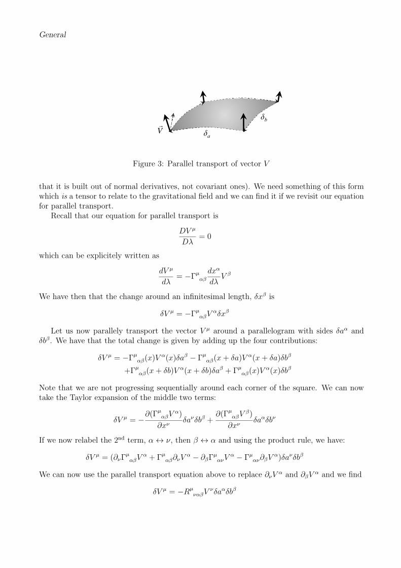
Figure 3: Parallel transport of vector V
that it is built out of normal derivatives, not covariant ones). We need something of this formwhich is a tensor to relate to the gravitational field and we can find it if we revisit our equationfor parallel transport.
Recall that our equation for parallel transport is
DV µ
Dλ= 0
which can be explicitely written as
dV µ
dλ= −Γµ
αβ
dxα
dλV β
We have then that the change around an infinitesimal length, δxβ is
δV µ = −ΓµαβV
αδxβ
Let us now parallely transport the vector V µ around a parallelogram with sides δaα andδbβ. We have that the total change is given by adding up the four contributions:
δV µ = −Γµαβ(x)V
α(x)δaβ − Γµαβ(x+ δa)V α(x+ δa)δbβ
+Γµαβ(x+ δb)V α(x+ δb)δaβ + Γµ
αβ(x)Vα(x)δbβ
Note that we are not progressing sequentially around each corner of the square. We can nowtake the Taylor expansion of the middle two terms:
δV µ = −∂(ΓµαβV
α)
∂xνδaνδbβ +
∂(ΓµαβV
β)
∂xνδaαδbν
If we now relabel the 2nd term, α ↔ ν, then β ↔ α and using the product rule, we have:
δV µ = (∂νΓµαβV
α + Γµαβ∂νV
α − ∂βΓµανV
α − Γµαν∂βV
α)δaνδbβ
We can now use the parallel transport equation above to replace ∂νVα and ∂βV
α and we find
δV µ = −RµναβV
νδaαδbβ
General Relativity and Cosmology 29
where
Rµναβ ≡ ∂αΓ
µβν − ∂βΓ
µαν + Γµ
αǫΓǫνβ − Γµ
ǫβΓǫνα (13)
We have that Rµναβ is the Riemann curvature tensor and it quantifies the curvature of a surface
(in this case space-time). If there was no curvature, the parallel transport around a closed loopwould bring a vector back onto itself. Rµ
ναβ is indeed a 4th rank tensor and depends on thesecond derivative. It should therefore be useful for teasing out the effects of a gravitationalfield. In fact we can define the Riemann curvature tensor in terms of covariant derivatives andvectors through:
(∇α∇β −∇β∇α)Vµ = Rµ
ναβVν
The Riemann tensor satisfies a number of symmetry properties:
Rµναβ = −Rµ
νβα
Rµναβ = −Rνµαβ
Rµναβ = Rαβµν
Rµναβ +Rµ
αβν +Rµβνα = 0
where the first index has been lowered using the metric: Rµναβ = gµǫRǫναβ. We also have the
Bianchi identity:
∇γRµναβ +∇βR
µνγα +∇αR
µνβγ = 0,
Finally, we can define the Ricci tensor and scalar:
Rαβ ≡ Rµαµβ
R ≡ gαβRαβ
11 Building the Einstein Field Equations
We now want to progress to the equations that tell us how the gravitational field is sourced. Wemay find a hint of how to construct the field equation from Newtonian gravity. In Newtoniangravity we have the Poisson equation:
∇2Φ = 4πGρ
Consider now two neighbouring particles, xi and xi = xi + N i in this gravitational field.Newton’s 2nd Law gives us
d2xi
dt2= −∂iΦ(x)
d2xi
dt2= −∂iΦ(x+N)
General Relativity and Cosmology 30
If we take the Taylor expansion of the 2nd equation we have, to lowest order:
d2N i
dt2= −∂j∂iΦN
j
We can define the tidal tensor:
Eij ≡ ∂j∂iΦ
so that
d2N i
dt2+ EijN
j = 0
(let us not worry about the fact that ”up” and ”down” indices don’t match just this once).We can call this the geodesic deviation equation for Newtonian gravity. Now let us revisit thePoisson equation; we have that it can be rewritten as
Eii = 4πGρ
We can now use this link between the geodesic deviation equation and the Poisson equationto construct the appropriate field equations for General Relativity. In constructing geodesics,we saw that the metric, gαβ played the role of gravitational potentials and we now need a setof equations which are invariant under coordinate transformations. Consider now a family ofgeodesics xα(λ, σ). We move along a geodesic by fixing σ and varying λ. We can move fromone geodesic to the next one by fixing λ and varying σ. We have the vector which is tangentto a given geodesic is simply:
T α =dxα
dλ|σ
while the vector which is orthogonal or normal to a geodesic at a point is
Nα =dxα
dσ|λ
We have that normal derivatives commute so ∂σTα = ∂λN
α. We can think of λ as a time coordi-nate and σ as a spatial coordinate, which means we can pick a coordinate system: (λ, σ, x2, x3).We then have that the tangent and normal vectors take a particularly simple form:
T α = δα0 Nα = δα1
Again, from the commutation of the normal derivatives we have Nβ∂βTα−T β∂βN
α = 0 whichremains true if we replace the normal derivatives by covariant derivatives:
Nβ∇βTα − T β∇βN
α = 0
Take the equation which relates the Riemann curvature tensor with the commutator of covariantderivatives:
(∇µ∇ν −∇ν∇µ)Tα = Rα
βµνTβ
General Relativity and Cosmology 31
Now contract it with Nα and T β:
NµT ν(∇µ∇νTα −∇ν∇µT
α) = RαβµνT
βT νNµ ≡ EαµN
µ (14)
We now have that
D2Nα
Dλ2= T µ∇µ(T
ν∇νNα)
which we can use the above commutation relation to rewrite as
D2Nα
Dλ2= T µ∇µ(N
ν∇νTα)
Using Leibnitz rule we have
D2Nα
Dλ2= T µN ν∇µ∇νT
α + T µ∇µNν∇νT
α
If we add this equation to equation 14 (and use the geodesic equation for T α) we find:
D2Nα
Dλ2+ Eα
βNβ = T µ∇µN
β∇βTα + T µNβ∇β∇µT
α
= T µ∇µNβ∇βT
α +Nβ∇β(Tµ∇µT
α)−Nβ∇βTµ∇µT
α
= T µ∇µNβ∇βT
α − T β∇βNµ∇µT
α = 0
We have then that the geodesic deviation equation in general relativity has a similar form tothat in Newtonian gravity but with a tidal tensor defined in equation 14. Clearly the Riemanncurvature (or some reduced version of it) must play the role that ∇2Φ plays in the Newtoniangravity. In fact, in the Newtonian limit we have
Eii = Ri0i0
so the Newton Poisson equation is of the form
RαβTαT β ≃ 4πGρ
The form of the equation is schematically ”Geometry ≃ Energy”, in other words, the matterwill source the geometry in someway. This is giving us a hint that the general relativisticequation should be of the form
Rαβ ∼ GTαβ
where Tαβ is a tensor which must be determined by the matter distribution.
12 The Energy-Momentum Tensor
We now need to construct the object, Tαβ which will be used for the General Relativistic Fieldequations. Cleary it must involve ρ. From Special Relativity we know that, if we change to a
General Relativity and Cosmology 32
moving frame, with velocity v and boost factor, γ, we have that ρ → γ2ρ. Which means thatρ transforms like a component of a 2nd rank tensor and hence fits nicely in an object such asTαβ. A first guess would be
T αβ = ρUαUβ
where Uα is the 4-velocity of the fluid, Uα ≡ γ(c,v). If we take the divergence of this tensor,we obtain a conservation equation:
∂αTαβ = 0
Setting γ = 1 we have two familiar conservation equations. First of all, conservation of mass:
∂ρ
∂t+ ∂i(ρv
i) = 0
and momentum
∂
∂t(ρvi) + ∂k(ρv
ivk) = 0
The latter equation can be reexpressed as the Euler equation for a pressureless fluid.We want to represent a more general, perfect fluid, one that include pressure, P and has
a form which is invariant under coordinate transformation- i.e. a proper tensor. This can beachieved with
T αβ = (ρ+P
c2)UαUβ + Pgαβ
where the 4-velocity of the fluid satisfies UαUα = −c2. In the local rest frame of the fluid, wehave U = (c,0). The energy-momentum conservation equation now becomes
∇αTαβ = 0
We can construct the energy-momentum tensor for just about anything: vector fields (like theelectric and magnetic fields), gases of particles described by distribution functions, fermions,scalar fields, etc.
13 The Einstein equations and the Newtonian Limit
Let us now attempt to construct the field equations which are tensorial and which have at most2nd derivatives. The only tensors at our disposal are, Rαβ, T αβ and gαβ. We also have twoscalars T ≡ gαβT
αβ and the Ricci scalar, R; it turns out that one of these will be redundant inwhat follows so we will discard T . The most general equation is
Rαβ = AT αβ + Bgαβ + CRgαβ (15)
where A, B and C are constants. From energy-momentum conservation we have that
∇αTαβ = 0
General Relativity and Cosmology 33
and the metricity condition gives us
∇µgαβ = 0
If we take the Bianchi identity
∇γRµναβ +∇βR
µνγα +∇αR
µνβγ = 0,
contract µ with α and multiply by gνγ we find
2∇νRνβ −∇βR = 0 (16)
We can replace this expression in Equation 15 to find C = 12. This allows us to define the
Einstein tensor:
Gαβ ≡ Rαβ − 1
2gαβR
We are left with two constants A and B so that
Gαβ = AT αβ +Bgαβ
What are these constants? Let us first focus on A. We can get an idea of where they comefrom by comparing the field equations with the Newton Poisson equation. To do so we haveto make two approximations. First of all we need to consider the weak field limit of gravity sothat we can expand the metric around a flat space, Minkowski space time:
gµν = ηµν + hµν
where |hµν | ≪ 1. Second, we will consider a time independent source with low speeds. Theenergy momentum tensor then becomes
T00 = ρc2 Tij ≃ 0
To first order in hµν the affine connections are
Γαµν ≃ 1
2ηαβ(∂µhβν + ∂νhµβ − ∂βhµν)
and the Riemann tensor becomes (note that we can discard products of Γs because they are2nd order)
Rαβµν =
1
2ηαγ(∂β∂µhνγ − ∂γ∂µhνβ − ∂β∂νhµγ + ∂ν∂γhµβ)
The Ricci tensor is then
Rβν = Rαβαν =
1
2ηαγ(∂β∂αhνγ − ∂γ∂αhνβ − ∂β∂νhαγ + ∂ν∂γhαβ)
General Relativity and Cosmology 34
To find A we will focus on the G00 component of the field equations. This means we need R00.We have chose a static source so that all derivatives with regards to 0 vanish. This leaves uswith
R00 = −1
2ηαγ∂γ∂αh00 ≃ −1
2∇2h00
Now taking g00 ≃ −(1 + 2 Φc2) we have
R00 =1
c2∇2Φ
For the Ricci scalar we can do the same. There is a trick we can use: assuming |Tij| ≃ 0 (asdeclared above), and setting B = 0 we have |Gij| ≃ 0 and so
Rij ≃1
2gijR =
1
2δijR
The Ricci scalar is
R = gαβRαβ ≃ ηαβRαβ = −R00 +Rii = −R00 +3
2R. (17)
So 2R00 = R and G00 = R00 − 12g00R ≃ R00 +R00 = 2R00 We can now replace it all in the field
equations:
2
c2∇2Φ = Aρc2
If this is to agree with the Poisson equation we must have
A =8πG
c4
Finally, it is a convention that we have B = −Λ and we call Λ the cosmological constant. Wethen have that the Einstein field equations are:
Gαβ =8πG
c4T αβ − Λgαβ (18)
We have completed our quest for a new theory of gravity. The set of Einstein Field Equa-tions given in equations 18 and the geodesic equations, given in equations 4 replace Newton’sUniversal law of gravitation and Newton’s 2nd law. In Einstein’s theory, the picture is different-as the American physicist John Archibald Wheeler said: ”Space tells matter how to move andmatter tells space how to curve.”
14 Black Holes
We now know how to, given a distribution of mass, derive the corresponding self-consistentmetric. The Einstein Field Equations are, of course, a tangled mess of non-linear equationswith 10 unknown functions of space time. It helps to consider symmetric configurations. We
General Relativity and Cosmology 35
now look at one such configuration, that of a spherically symmetric, static metric in vacuum.If we write such a metric in spherical polar coordinates we have
ds2 = −c2f(r)dt2 + g(r)dr2 − e(r)dtdr + h(r)(dθ2 + sin2 θdφ2)
With a judicious redefinition of r and t we can eliminate e(r) and h(r) and we can then workwith
ds2 = −c2f(r)dt2 + g(r)dr2 + r2(dθ2 + sin2 θdφ2)
We will solve the Einstein Field Equations in empty space, where Tµν = 0. The equationscan be rewritten as Rµν = 0 and so the challenge is to construct the Ricci tensor for such aspace time with
g00 = −f(r)
grr = g(r)
gθθ = r2
gφφ = r2 sin2 θ
There are 9 non-zero connection coefficients and these are:
Γr00 = −1
2grr∂rg00 =
1
2
f ′
g
Γ00r =
1
2g00∂rg00 = −1
2
f ′
f
Γrrr =
1
2grr∂rgrr =
1
2
g′
g
Γrθθ = −1
2grr∂rgθθ = −r
g
Γrφφ = −1
2grr∂rgφφ = −r sin2 θθ
g
Γθθr =
1
2gθθ∂rgθθ =
1
r
Γθφφ = −1
2gθθ∂θgφφ = − sin θ cos θ
Γφφr =
1
2gφφ∂rgφφ =
1
r
Γφφθ = −1
2gφφ∂θgφφ =
cos θ
sin θ
We now need expressions for Rµν which are
R00 =1
2
f ′′
g+
1
4
f ′f ′
fg− 1
4
f ′g′
g2+
1
2r
f ′
g
Rrr =1
2
f ′′
f+
1
4
f ′f ′
f 2− 1
4
f ′g′
fg+
1
2r
g′
g
Rθθ =1
g− 1 +
r
2g
(
f ′
f− g′
g
)
Rφφ = sin2 θRθθ
General Relativity and Cosmology 36
There are no off-diagonal terms and there are only three equations. We can now take the firsttwo to find
g
fR00 +Rrr = −1
r
(
f ′
f+
g′
g
)
= 0
This easily solved to give fg = α where α is a constant. Replacing g in the Rθθ = 0 we find
f + rf ′ = α
which integrated gives us
f = α(1 +κ
r)
Matching this expression to the weak field limit (i.e. the Newtonian regime) we find α = 1 andκ = −2GM/c2r so that the final solution is the Schwarzschild metric:
ds2 = −(
1− 2GM
c2r
)
c2dt2 +(
1− 2GM
c2r
)−1
dr2 + r2dθ2 + r2 sin2(θ)dφ2
which we have used extensively throughout these lecture notes.We have focused on the weak field region of this space time but let us try an understand a
bit more about its peculiarities. For a start, something odd seems to happen at rS = 2GM/c2,known as the Schwarzschild radius: the metric seems to blow up. Nevertheless we know thatthe Ricci tensor is 0 and if we calculate the Riemann tensor we find that
RαβµνRαβµν = 12r2Sr4
i.e. it is also finite. It turns out that at rS we don’t have a genuine space time singularity buta coordinate singularity. This doesn’t mean that odd things don’t happen at that, or near thatpoint.
Let us consider geodesics in this space time. Using the geodesics that we derived above, wehave that the radial equation is
r = −GM
r2+
h2
r3
(
1− 3GM
c2r
)
We can find the stable minima of the left hand side (to which we can associate circular orbits)to find that they are at
r =2h2 ±
√
4h4 − 12r2Sc2h2
2rSc2
There is clearly a limit of h below which there is no solution and it is given by h2 = 3r2Sc2.
This corresponds to the Innermost Stable Circular Orbit: rISCO = 3rs. There are no circularorbits with smaller radii, all orbits are inspiralling towards rS. Interestingly enough, outsidethis orbit, circular orbits do satisfy Kepler’s law: (dφ/dt)2 = GM/r3.
General Relativity and Cosmology 37
Let us now study what happens to an infalling particle. We can set h = 0 to find
r = −rSc2
2r2
Taking r = 0 at r → ∞ we find an integral of motion
r2 =rSc
2
2r
Integrating this equation, taking τ = 0 at r = r0 and defining ξ = r/rS we find
cτ
rS=
2
3(ξ
3/20 − ξ3/2)
Taking xi = 0 we find that it take a finite amount of proper time for a particle to reach r = 0from any radius (within or without the Schwarazschild radius). If, however, we wish to findthe amount of time elapsed for an observer at infinity, we need to integrate
dr
dt= −
(
rsc2
r
)1/2 (
1− rSr
)
which gives
ct
rS=
2
3(ξ
3/20 − ξ3/2) + 2(ξ
1/20 − ξ1/2) + ln
∣
∣
∣
∣
∣
∣
(ξ1/2 + 1)(ξ1/20 − 1)
(ξ1/2 − 1)(ξ1/20 + 1)
∣
∣
∣
∣
∣
∣
If we the endpoint to be the Schwarzschild radius (i.e. ξ = 1), we have that ct → ∞. In otherwords, from an external observer it takes an infinite amount of time for the particle to fall in.
We can solve the geodesic equations for radial light rays by looking directly at the metric.We then have
(
1− rSr
)1/2
cdt = ±(
1− rSr
)−1/2
dr
which can be rewritten as
cdt
dr= ±(1− rS
r)−1
and integrated to give
ct = ±r ± rs ln |r
rS− 1|+ r0
where r0 is a constant of integration. With rS we have the usual light cones with which we arefamiliar in Minkowski space. This is also approximately true for r/rS ≫ 1. But for r/rS, thelight cone ”tips over” so that all forward moving particles necessarily move inwards towardsr = 0. It is not possible to causally exit the Schwarzschild radius. The Schwarzschild radiusworks as a horizon beyond which we can’t see anything. It is an event horizon.
General Relativity and Cosmology 38
Finally, such strong effects may still be at play even if the object is not a black hole. Verydense objects like neutrons stars can be a good laboratory for testing gravity. And indeed,Binary pulsars are incredibly useful astronomical objects that can be used to place very tightconstraints on General Relativity. Pulsars are rapidly rotating neutrons stars that emit a beamof electromagnetic radiation, and were first observed in 1967. When these beams pass over theEarth, as the star rotates, we detect regular pulses of radiation. The first pulsar observed ina binary system was PSR B1913+16 in 1974, by Hulse and Taylor. The rotational period ofthis pulsar is about 59ms as it orbits around another neutron star. Binary pulsars are highlyrelativistic. For example the Hulse-Taylor pulsar precesses relativistically more than 30 000times faster than the Mercury-Sun system. They are also a source of gravitational radiation,i.e. waves in space time that propagate away from the system and take energy away. We canpredict how much energy in gravitational radiation a binary system will emit, in the contextof General Relativity- it agrees almost perfectly with the angular momentum decay observedin the Hulse-Taylor pulsar. Indeed the Hulse-Taylor pulsar is an incredibly rich laboratoryfor General Relativity. At least 5 General Relativistic effects have been measured: orbitalprecession (also known as periastron advance), the rate of change of the orbital period, thegravitational redshift and two versions of the Shapiro time-delay effects.
15 Homogeneous and Isotropic Space- Times
The Einstein Field Equations are a tangled mess of ten nonlinear partial differential equations.They are incredibly hard to solve and for almost a century there have been many attemptsat finding solutions which might describe real world phenomena. For the remainder of theselectures we are going to focus on one set of solutions which apply in a very particular regime.We will solve the Field Equations for the whole Universe under the assumption that it ishomogeneous and isotropic.
For many centuries we have grown to believe that we don’t live in a special place, thatwe are not at the center of the Universe. And, oddly enough, this point of view allows us tomake some far reaching assumptions. So for example, if we are insignificant and, furthermore,everywhere is insignificant, then we can assume that at any given time, the Universe looksthe same everywhere. In fact we can take that statement to an extreme and assume that atany given time, the Universe looks exactly the same at every single point in space. Such aspace-time is dubbed to be homogeneous.
There is another assumption that takes into account the extreme regularity of the Universeand that is the fact that, at any given point in space, the Universe looks very much the samein whatever direction we look. Again such an assumption can be taken to an extreme so thatat any point, the Universe look exactly the same, whatever direction one looks. Such a spacetime is dubbed to be isotropic.
Homogeneity and isotropy are distinct yet inter-related concepts. For example a universewhich is isotropic will be homogeneous while a universe that is homogeneous may not beisotropic. A universe which is only isotropic around one point is not homogeneous. A universethat is both homogeneous and isotropic is said to satisfy the Cosmological Principle. It isbelieved that our Universe satisfies the Cosmological Principle.
Homogeneity severely restrict the metrics that we are allowed to work with in the Einstein
General Relativity and Cosmology 39
field equation. For a start, they must be independent of space, and solely functions of time.Furthermore, we must restrict ourselves to spaces of constant curvature of which there are onlythree: a flat euclidean space, a positively curved space and a negatively curved space. We willlook at curved spaces in a later lecture and will restrict ourselves to a flat geometry here.
The metric for a flat Universe takes the following form:
ds2 = −c2dt2 + a2(t)[(dx1)2 + (dx2)2 + (dx3)2]
We call a(t) the scale factor and t is normally called cosmic time or physical time. The energymomentum tensor must also satisfy homogeneity and isotropy. If we consider a perfect fluid,we restrict ourselves to
T αβ = (ρ+P
c2)UαUβ + Pgαβ
with Uα = (c, 0, 0, 0) and ρ and P are simply functions of time. Note that both the metric andthe energy-momentum tensor are diagonal. So
g00 = −1 gij = a2(t)δij
T00 = ρc2 Tij = a2Pδij
As we shall see, with this metric and energy-momentum tensor, the Einstein field equations aregreatly simplified. We must first calculate the connection coefficients. We have that the onlynon-vanishing elements are (and from now one we will use . = d
dti.e. not to be confused with
ddλ
that we have used previously for the geodesic equations):
Γ0ij =
1
caaδij
Γi0j =
1
c
a
aδij
and the resulting Ricci tensor is
R00 = − 3
c2a
aR0i = 0
Rij =1
c2(aa+ 2a2)δij
Again, the Ricci tensor is diagonal. We can calculate the Ricci scalar:
R = −R00 +1
a2Rii =
1
c2
[
6a
a+ 6
(
a
a
)2]
to find the two Einstein Field equations:
G00 = R00 −1
2Rg00 =
8πG
c4T00 ⇔ 3
(
a
a
)2
= 8πGρ
Gij = Rij −1
2Rgij =
8πG
c4Tij ⇔ −2aa− a2 =
8πG
c2a2P
General Relativity and Cosmology 40
We can use the first equation to simplify the 2nd equation to
3a
a= −4πG(ρ+ 3
P
c2)
These two equations can be solved to find how the scale factor, a(t), evolves as a function oftime. The first equation is often known as the Friedman-Robertson-Walker equation or FRWequation and the metric is one of the three FRW metrics. The latter equation in a is known asthe Raychauduri equation.
Both of the evolution equations we have found are sourced by ρ and P . These quantitiessatisfy a conservation equation that arises from
∇αTαβ = 0
and in the homogeneous and isotropic case becomes
ρ+ 3a
a(ρ+
P
c2) = 0
It turns out that the FRW equation, the Raychauduri equation and the energy-momentumconservation equation are not independent. It is a straightforward exercise to show that youcan obtain one from the other two. We are therefore left with two equations for three unknowns.
One has to decide what kind of energy we are considering and in a later lecture we willconsider a variety of possibilities. But for now, we can hint at a substantial simplification. Ifwe assume that the system satisfies an equation of state, so P = P (ρ) and, furthermore that itis a polytropic fluid we have that
P = wρc2 (19)
where w is a constant, the equation of state of the system.
16 Properties of a Friedman Universe I
We can now explore the properties of these evolving Universes. Let us first do something verysimple. Let us pick two objects (galaxies for example) that lie at a given distance from eachother. At time t1 they are at a distance r1 while at a time t2, they are at a distance r2. Wehave that during that time interval, the change between r1 and r2 is given by
r2r1
=a(t2)
a(t1)
and, because of the cosmological principle, this is true whatever two points we would havechosen. It then makes to sense to parametrize the distance between the two points as
r(t) = a(t)x
where x is completely independent of t. We can see that we have already stumbled upon xwhen we wrote down the metric for a homogeneous and isotropic space time. It is the set of
General Relativity and Cosmology 41
coordinates (x1, x2, x3) that remain unchanged during the evolution of the Universe. We knownthat the real, physical coordinates are multiplied by a(t) but (x1, x2, x3) are time independentand are known as conformal coordinates. We can work out how quickly the two objects weconsidered are moving away from each other. We have that their relative velocity is given by
v = r = ax =a
aax =
a
ar ≡ Hr
In other words, the recession speed between two objects is proportional to the distance betweenthem. This equality applied today (at t0) is
v = H0r
and is known as Hubble’s Law where H0 is the Hubble constant and is given by H0 = 100h kms−1 Mpc−1 and h is a dimensionless constant which is approximately h ≃ 0.7.
How can we measure velocities in an expanding universe? Consider a photon with wave-length λ being emitted at one point and observed at some other point. We have that theDoppler shift is given by
λ′ ≃ λ(1 +v
c)
We can rewrite it in a differential form
dλ
λ≃ dv
c=
a
a
dr
c=
a
adt =
da
a
and integrate to find λ ∝ a. We therefore have that wave lengths are stretched with theexpansion of the Universe. It is convenient to define the factor by which the wavelength isstretched by
z =λr − λe
λe
→ 1 + z ≡ a0a
where a0 is the scale factor today (throughout these lecture notes we will choose a conventionin which a0 = 1). We call z the redshift.
For example, if you look at Figure 4 you can see the spectra measured from a galaxy; afew lines are clearly visible and identifiable. Measured in the laboratory on Earth (top panel),these lines will have a specific set of wavelengths but measured in a specific, distant, galaxy(bottom panel) the lines will be shifted to longer wavelengths. Hence a measurement of theredshift (or blueshift), i.e. a measurement of the Doppler shift, will be a direct measurementof the velocity of the galaxy.
The American astronomer, Edwin Hubble measured the distances to a number of distantgalaxies and measured their recession velocities. The data he had was patchy, as you can seefrom Figure 5, but he was able to discern a a pattern: most of the galaxies are moving awayfrom us and the further away they are, the faster they are moving. With more modern data,this phenomenon is striking, as you can see in the Figure 5. The data is neatly fit by a law ofthe form
v = H0r
where H0 is a constant (known as Hubble’s constant). Current measurements of this constantgive us H0 = 67 km s−1 Mpc−1.
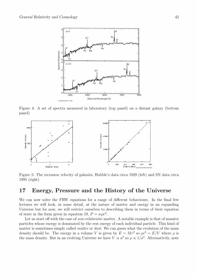
General Relativity and Cosmology 42
Figure 4: A set of spectra measured in laboratory (top panel) on a distant galaxy (bottompanel)
Figure 5: The recession velocity of galaxies, Hubble’s data circa 1929 (left) and SN data circa1995 (right)
17 Energy, Pressure and the History of the Universe
We can now solve the FRW equations for a range of different behaviours. In the final fewlectures we will look, in some detail, at the nature of matter and energy in an expandingUniverse but for now, we will restrict ourselves to describing them in terms of their equationof state in the form given in equation 19, P = wρc2.
Let us start off with the case of non-relativistic matter. A notable example is that of massiveparticles whose energy is dominated by the rest energy of each individual particle. This kind ofmatter is sometimes simply called matter or dust. We can guess what the evolution of the massdensity should be. The energy in a volume V is given by E = Mc2 so ρc2 = E/V where ρ isthe mass density. But in an evolving Universe we have V ∝ a3 so ρ ∝ 1/a3. Alternatively, note
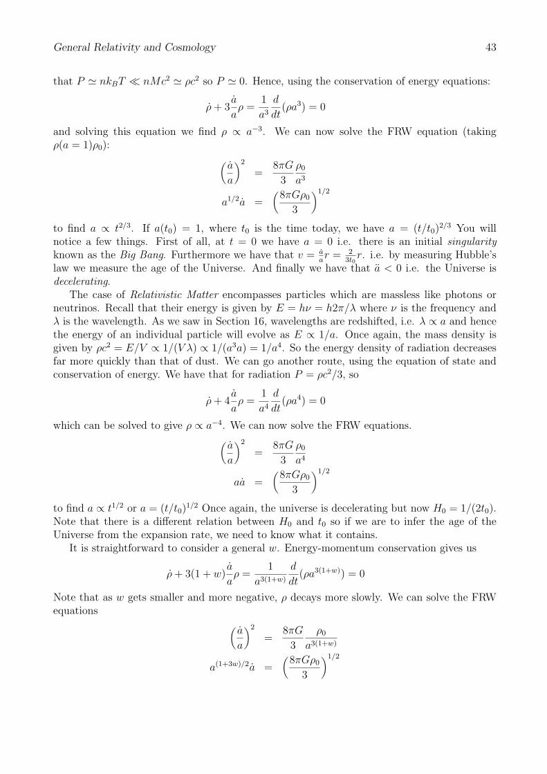
General Relativity and Cosmology 43
that P ≃ nkBT ≪ nMc2 ≃ ρc2 so P ≃ 0. Hence, using the conservation of energy equations:
ρ+ 3a
aρ =
1
a3d
dt(ρa3) = 0
and solving this equation we find ρ ∝ a−3. We can now solve the FRW equation (takingρ(a = 1)ρ0):
(
a
a
)2
=8πG
3
ρ0a3
a1/2a =(
8πGρ03
)1/2
to find a ∝ t2/3. If a(t0) = 1, where t0 is the time today, we have a = (t/t0)2/3 You will
notice a few things. First of all, at t = 0 we have a = 0 i.e. there is an initial singularityknown as the Big Bang. Furthermore we have that v = a
ar = 2
3t0r. i.e. by measuring Hubble’s
law we measure the age of the Universe. And finally we have that a < 0 i.e. the Universe isdecelerating.
The case of Relativistic Matter encompasses particles which are massless like photons orneutrinos. Recall that their energy is given by E = hν = h2π/λ where ν is the frequency andλ is the wavelength. As we saw in Section 16, wavelengths are redshifted, i.e. λ ∝ a and hencethe energy of an individual particle will evolve as E ∝ 1/a. Once again, the mass density isgiven by ρc2 = E/V ∝ 1/(V λ) ∝ 1/(a3a) = 1/a4. So the energy density of radiation decreasesfar more quickly than that of dust. We can go another route, using the equation of state andconservation of energy. We have that for radiation P = ρc2/3, so
ρ+ 4a
aρ =
1
a4d
dt(ρa4) = 0
which can be solved to give ρ ∝ a−4. We can now solve the FRW equations.(
a
a
)2
=8πG
3
ρ0a4
aa =(
8πGρ03
)1/2
to find a ∝ t1/2 or a = (t/t0)1/2 Once again, the universe is decelerating but now H0 = 1/(2t0).
Note that there is a different relation between H0 and t0 so if we are to infer the age of theUniverse from the expansion rate, we need to know what it contains.
It is straightforward to consider a general w. Energy-momentum conservation gives us
ρ+ 3(1 + w)a
aρ =
1
a3(1+w)
d
dt(ρa3(1+w)) = 0
Note that as w gets smaller and more negative, ρ decays more slowly. We can solve the FRWequations
(
a
a
)2
=8πG
3
ρ0a3(1+w)
a(1+3w)/2a =(
8πGρ03
)1/2
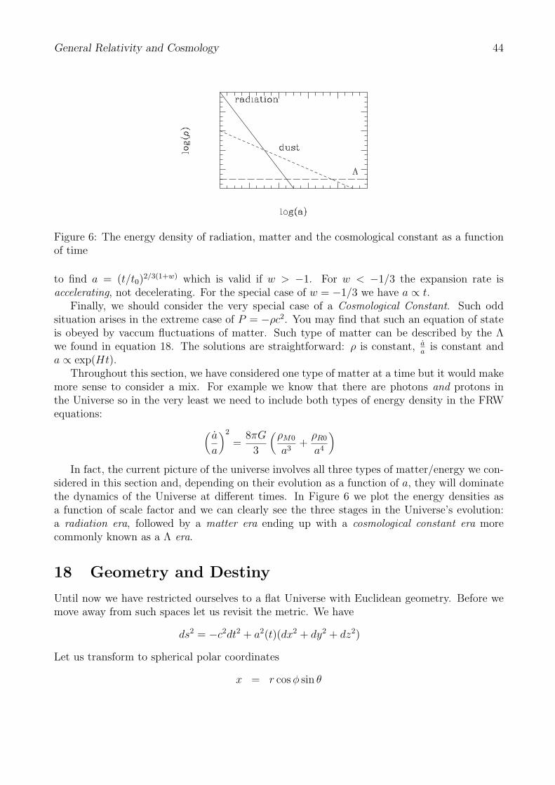
General Relativity and Cosmology 44
Figure 6: The energy density of radiation, matter and the cosmological constant as a functionof time
to find a = (t/t0)2/3(1+w) which is valid if w > −1. For w < −1/3 the expansion rate is
accelerating, not decelerating. For the special case of w = −1/3 we have a ∝ t.Finally, we should consider the very special case of a Cosmological Constant. Such odd
situation arises in the extreme case of P = −ρc2. You may find that such an equation of stateis obeyed by vaccum fluctuations of matter. Such type of matter can be described by the Λwe found in equation 18. The solutions are straightforward: ρ is constant, a
ais constant and
a ∝ exp(Ht).Throughout this section, we have considered one type of matter at a time but it would make
more sense to consider a mix. For example we know that there are photons and protons inthe Universe so in the very least we need to include both types of energy density in the FRWequations:
(
a
a
)2
=8πG
3
(
ρM0
a3+
ρR0
a4
)
In fact, the current picture of the universe involves all three types of matter/energy we con-sidered in this section and, depending on their evolution as a function of a, they will dominatethe dynamics of the Universe at different times. In Figure 6 we plot the energy densities asa function of scale factor and we can clearly see the three stages in the Universe’s evolution:a radiation era, followed by a matter era ending up with a cosmological constant era morecommonly known as a Λ era.
18 Geometry and Destiny
Until now we have restricted ourselves to a flat Universe with Euclidean geometry. Before wemove away from such spaces let us revisit the metric. We have
ds2 = −c2dt2 + a2(t)(dx2 + dy2 + dz2)
Let us transform to spherical polar coordinates
x = r cosφ sin θ
General Relativity and Cosmology 45
y = r sinφ sin θ
z = r cos θ
and rewrite the metric
ds2 = −c2dt2 + a2(t)(dr2 + r2dθ2 + r2 sin2 θdφ2)
We could in principle work out the FRW and Raychauduri equations in this coordinate system.Let us now consider a 3 dimensional surface that is positively curved. In other words, it is
the surface of a 3 dimensional hypersphere in a fictitious space with 4 dimensions. The equationfor the surface of a sphere in this 4 dimensional space, with coordinates (X, Y, Z,W ), is
X2 + Y 2 + Z2 +W 2 = R2
Now in the same way that we can construct spherical coordinates in three dimensions, we canbuild hyperspherical coordinates in 4 dimensions:
X = R sinχ sin θ cosφ
Y = R sinχ sin θ sinφ
Z = R sinχ cos θ
W = R cosχ
We can now work out the line element on the surface of this hyper-sphere
ds2 = dX2 + dY 2 + dZ2 + dW 2 = R2[
dχ2 + sin2 χ(dθ2 + sin2 θdφ2)]
Note how different it is from the flat geometry. If we transform R sinχ into r for it all to agreewe have that
dχ2 =dr2
R2 − r2
We can now repeat this exercise for 3-D surface with negative curvature- a hyper-hyperboloideso to speak. In our fictitious 4-D space (not to be confused with space time), we have that thesurface is defined by
X2 + Y 2 + Z2 −W 2 = −R2
Let us now change to a good coordinate system for that surface:
X = R sinhχ sin θ cosφ
Y = R sinhχ sin θ sinφ
Z = R sinhχ cos θ
W = R coshχ
The line element on that surface will now be
ds2 = dX2 + dY 2 + dZ2 + dW 2 = R2[
dχ2 + sinh2 χ(dθ2 + sin2 θdφ2)]
General Relativity and Cosmology 46
We can replace R sinhχ by r to get
dχ2 =dr2
R2 + r2
We can clearly write all three space time metrics (flat, hyperspherical, hyper-hyperbolic) ina unified way. If we take r = R sinχ for the positively curved space and r = R sinhχ for thenegatively curved space we have
ds2 = −c2dt2 + a2(t)
[
d2r
1− kr2+ r2(dθ2 + sin2 θdφ2)
]
(20)
where k is positive, zero or negative for spherical, flat or hyperbolic geometries, and |k| = 1/R2.We can now repeat the calculation we undertook for a flat geometry and find the con-
nection coefficients, Ricci tensor and scalar and the evolution equations. Take the metricgαβ = diag(−1, a2
1−kr2, a2r2, a2r2 sin θ2) and note that for this choice of coordinates, the i and j
labels now run over r, θ and φ. We find that the connection coefficients are:
Γ0ij =
1
caagij
Γi0j =
1
c
a
aδij
Γijk = Γi
jk
where gij and Γ are the metric and connection coefficients of the conformal 3-space (that is ofthe 3-space with the conformal factor, a, divided out):
Γrrr =
kr
1− kr2
Γrθθ = −r(1− kr2)
Γrφφ = −(1− kr2)r sin2(θ)
Γθθr =
1
r
Γθφφ =
− sin(2θ)
2
Γφφr =
1
r
Γφθφ =
1
tan(θ)
The Ricci tensor and scalar can be combined to form the Einstein tensor
G00 = 3a2 + kc2
c2a2
Gij = −2aa+ a2 + kc2
c2gij
(21)
General Relativity and Cosmology 47
while the energy-momentum tensor is
T00 = ρc2
Tij = a2P gij
Combining them gives us the Friedman equation
(
a
a
)2
=8πG
3ρ− kc2
a2
while the Raychauduri equations remains as
3a
a= −4πG
3(ρ+ 3
P
c2)
Let us now explore the consequences of the overall geometry of the Universe, i.e. the termproportional to k in the FRW equations: For simplicity, let us consider a dust filled universe.We can see that the term proportional to k will only be important at late times, when itdominates over the energy density of dust. In other words, in the universe we can say thatcurvature dominates at late times. Let us now consider the two possibilities. First of all, let ustake k < 0. We then have that
(
a
a
)2
=8πG
3ρ+
|k|c2a2
When the curvature dominates we have that(
a
a
)2
=|k|c2a2
so a ∝ t. In this case, the scale factor grows at the speed of light. We can also consider k > 0.From the FRW equations we see that there is a point, when 8πG
3ρ = kc2
a2and therefore a = 0
when the Universe stops expanding. At this point the Universe starts contracting and evolvesto a Big Crunch. Clearly geometry is intimately tied to destiny. If we know the geometry ofthe Universe we know its future.
There is another way we can fathom the future of the Universe. If k = 0, there is a strictrelationship between H = a
aand ρ. Indeed from the FRW equation we have
H2 =(
a
a
)2
=8πG
3ρ → ρ = ρc ≡
3H2
8πG
We call ρc the critical density. It is a function of a. If we take H0 = 100hKm s−1 Mpc−1, wehave that
ρc = 1.9× 10⁻²⁶h2kgm−3
which corresponds to a few atoms of Hydrogen per cubic meter. Compare this with the densityof water which is 103 kg m−3. Now let us take another look at the FRW equation and rewriteit as
1
2a2 − 4πG
3ρa2 = −1
2kc2
General Relativity and Cosmology 48
which has the form Etot = U +K and we equate Etot to −kc2 so that K is the kinetic energy,U is the gravitational energy. We see that if ρ = ρc, it corresponds to the total energy of thesystem being 0, i.e. kinetic and gravitational energy balance themselves out perfectly. Let uslook at the case of nonzero k.
k < 0 ρ < ρc and therefore total energy is positive, kinetic energy wins out and the Universeexpands at a constant speed.
k > 0 ρ > ρc and the total energy is negative, gravitational energy wins out and the Universerecollapses.
We recover an important underlying principle behind all this, the geometry is related to theenergy density.
It is convenient to define a more compact notation. The fractional energy density or densityparameter. We define
Ω ≡ ρ
ρc
It will be a function of a and we normally express its value today as Ω0. If there are variouscontributions to the energy density, we can define the fractional energy densities of each one ofthese contributions. For example
ΩR ≡ ρRρc
ΩM ≡ ρMρc
· · ·
It is convenient to define two additional Ωs:
ΩΛ ≡ Λ
3H2
Ωk ≡ − kc2
a2H2
and we have Ω:
Ω = ΩR + ΩM + ΩΛ
We now have
Ω < 1 : ρ < ρc, k < 0, Universe is open (hyperbolic)
Ω = 1 : ρ = ρc, k = 0, Universe is flat (Euclidean)
Ω > 1 : ρ > ρc, k > 0, Universe is closed (spherical)
If we divide the FRW equation through by ρc we find that it can be rewritten as
H2(a) = H20
[
ΩM0
a3+
ΩR0
a4+
ΩK0
a2+ ΩΛ
]
(22)
where the subscript ”0” indicates that these quantities are evaluated at t0. We will normallydrop the subscript when referring to the various Ωs evaluated today. When we refer to the Ωsat different times, we will explicitely say so or add an argument (for example ΩM(a) or ΩM(z)).
General Relativity and Cosmology 49
How does Ω evolve? Without loss of generality, let us consider a Universe with dust, takethe FRW equations and divide by H2 to obtain
Ω− 1 =kc2
a2H2∝ kt2/3
I.e., if Ω 6= 1, it is unstable and driven away from 1. The same is true in a radiation dominateduniverse and for any decelerating Universe: Ω = 1 is an unstable fixed point and, as we sawabove, curvature dominates at late times.
19 Properties of a Friedman Universe I
Let us revisit the properties of a FRW universe, now that we know a bit more about the theevolution of the scale factor. Distances play an important role if we are to map out its behaviourin detail. We have already been exposed to Hubble’s law
v = H0d
from which we can extract Hubble’s constant. From Hubble’s constant we can define a Hubbletime
tH =1
H0
= 9.78× 10⁹ h−1 yr
and the Hubble distance
DH =c
H0
= 3000 h−1 Mpc
These quantities set the scale of the Universe and give us a rough idea of how old it is and howfar we can see. They are only rough estimates and to get a firmer idea of distances and ages,we need to work with the metric and FRW equations more carefully.
To actually figure out how far we can see, we need to work out how far a light ray travelsover a given period of time. To be specific, what is the distance, DM to a galaxy that emitteda light ray at time t, which reaches us today? Let us look at the expression for the metric usedin equation 20 for a light ray. We have that
dr2
1− kr2=
c2dt2
a2(t)(23)
The time integral gives us the comoving distance:
DC = c∫ t0
t
dt′
a(t′)
From equation 22 we have that −k = Ωk/D2H . Performing the radial integral (and assuming
the observer is at r = 0 we have
∫ DM
0
dr√1− kr2
=
DH√Ωk
sinh−1[√ΩkDM/DH ] for Ωk > 0
DM for Ωk = 0DH√|Ωk|
sin−1[√
|Ωk|DM/DH ] for Ωk < 0
General Relativity and Cosmology 50
so we find an expression for the proper motion distance (also known as the transverse comovingdistance, DM in terms of the comoving distance)
DM =
DH√Ωk
sinh[√ΩkDC/DH ] for Ωk > 0
DC for Ωk = 0DH√|Ωk|
sin[√
|Ωk|DC/DH ] for Ωk < 0
Suppose now we we look at an object of a finite size which is transverse to our line of sightand lies at a certain distance from us. If we divide the physical transverse size of the object bythe angle that object subtends in the sky (the angular size of the object) we obtain the angulardiameter distance:
DA =DM
1 + z
Hence, if we know that size of an object and its redshift we can work out, for a given Universe,DA.
Alternatively, we may know the brightness or luminosity of an object at a given distance.We know that the flux of that object at a distance DL is given by
F =L
4πD2L
DL is aptly known as the luminosity distance and is related to other distances through:
DL = (1 + z)DM = (1 + z)2DA
It turns out that, in astronomy, one often works with a logarithmic scale, i.e. with magnitudes.One can define the distance modulus:
DM ≡ 5 log
(
DL
10 pc
)
and it can be measured from the apparent magnitude m (related to the flux at the observer)and the absolute magnitude M (what it would be if the observer was at 10 pc from the source)through
m = M +DM
We now have a plethora of distances which can be deployed in a range of different observa-tions. They clearly depend on the universe we are considering, i.e. on the values of H0, and thevarious Ωs. While Ωk will dictate the geometry, Dc will depend on how the Universe evolves. Itis useful to rewrite Dc in a few different ways. It is useful to use the FRW in the form presentedin equation 22. We can transform the time integral in Dc to an integral in a:
DC =∫ t0
t
cdt′
a(t′)= c
∫ 1
a
da
a2H(a)= DH
∫ 1
a
da
a2√
ΩM/a3 + ΩR/a4 + Ωk/a2 + ΩΛ
General Relativity and Cosmology 51
An interesting question is how far has light travelled, from the big bang until now? Thisis known as the particle horizon, rP and a naive estimate would be rP ≃ ct0 but that doesn’ttake into account the expansion of space time. The correct expression is given above and it is
rP = DC(0)
where the argument implies that it is evaluated from t = 0 to t = t0. Applying it now to thesimple case of a dust filled, flat Universe. We have that
rP = 3ct0
Unsurprisingly, the expansion leads to an extra factor.We could ask a different question: how far can light travel from now until the infinite future,
i.e. how much will we ever see of the current Universe. Known as the event horizon it is by theintegral of equation 23 from t0 until ∞. For example in a flat Universe we have
rE =∫ ∞
t0
cdt′
a(t′)
For a dust or radiation dominated universe we have that rE = ∞ but this is not so for a universedominated by a cosmological constant.
We have been focusing on distances but we can also improve our estimate of ages. Wedefined the Hubble time above and that is a rough estimate of the age of the Universe. To dobetter we need to resort to the FRW equations again, as above we have that a = aH so
dt =da
aH→∫ t0
0dt =
∫ 1
0
da
aH= t0
which, combined with equation 22 gives us
t0 =1
H0
∫ 1
0
da
a√
ΩM/a3 + ΩR/a4 + Ωk/a2 + ΩΛ
We can use the above equation quite easily. For a flat, dust dominated Universe we findt0 = 2/(3H0). If we now include a cosmological constant as well, we find
t0 = H−10
∫ 1
0
da
a√
ΩM/a3 + ΩΛ
At ΩΛ = 0 we simply retrieve the matter dominated result, but the larger ΩΛ is, the older theUniverse. To understand why, recall the Raychauduri equation for this Universe:
a
a= −4πG
3ρ+
Λ
3
Divide by H20 and we have that the deceleration parameter
q0 ≡ −a(t0)a(t0)
a2(t0)=
1
2ΩM − ΩΛ
General Relativity and Cosmology 52
If ΩM +ΩΛ = 1 then q0 =32ΩM −1. If ΩM < 2
3we have q0 < 0 and the Universe is accelerating.
This lets us understand why the Universe is older. Take a ΩΛ = 0 and a ΩΛ > 0 which bothhave the same expansion rate today. The latter is accelerating which means it was expandingmore slowly in the past than the former. This means it must have taken longer to reach itscurrent speed and hence is older. Furthermore we can see that our inference about the Universedepends on our knowledge of the various Ωs. In other words, if we want to measure the age ofthe Universe we must also measure the density in its various components.
Finally, let us revisit Hubble’s law. We worked out the relationship between velocities anddistance for two objects which were very close to each other. If we want to consider objectswhich are further apart (not too distant galaxies) we can Taylor expand the scale factor today,we find that
a(t) = a(t0) + a(t0)[t− t0] +1
2a(t0)[t− t0]
2 + · · ·
Assume that the distance to the emitter at time t is roughly given by d =≃ c(t0 − t) we canrewrite it as
(1 + z)−1 = 1−H0d
c− q0H
20
2
(
d
c
)2
+ · · ·
For q0 = 0 and small z we recover the Hubble law, cz = H0d. As we go to higher redshift, thisis manifestly not good enough.
20 The Cosmological Distance ladder
Given our model of a range of possible universes, we would like to pin down which set ofcosmological parameters (like t0, H0, ΩM , · · ·) correspond to our Universe. We can ask questionslike: what is the age of the Universe, is it accelerating or decelerating, what is its density andgeometry? Interestingly enough, all these questions must be answered together and to do sowe need to go out, observe and measure.
The first step is to map out the Universe and measure distances and redshifts accurately.By far the easiest quantity to measure is the redshift. By looking at the shift in the spectra ofknown elements it is possible to infer the recession velocity of the galaxy directly. Measuringdistances is much harder. The most direct method is to use parallax to measure the distanceto a star. Let us remember what you do here. Imagine that you look at an object in the sky. Itcan be described in terms of two angles. It has a position on the celestial sphere. Now imaginethat we move a distance 2d from where we were. The object may move an angle θ from whereit was. The angle that it has moved will be related to the distance D and displacement d. If wesay θ = 2α then we have tanα = d
DIf α is small then we can use the small angle approximation
to get
α =d
D
The motion of the earth around the sun gives us a very good baseline with which to measuredistance. The distance from the earth to the sun is 1 AU so we have that D = 1
αwhere α is
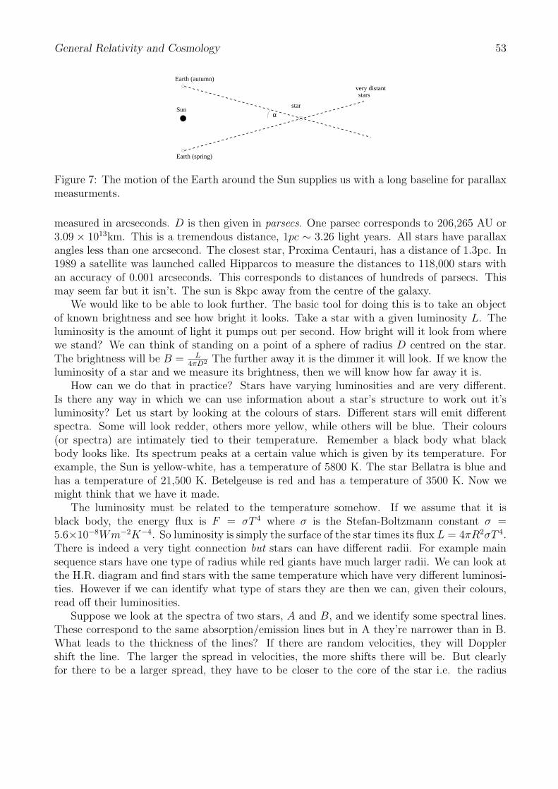
General Relativity and Cosmology 53
Sun
Earth (spring)
Earth (autumn)
star
very distantstars
α
Figure 7: The motion of the Earth around the Sun supplies us with a long baseline for parallaxmeasurments.
measured in arcseconds. D is then given in parsecs. One parsec corresponds to 206,265 AU or3.09 × 1013km. This is a tremendous distance, 1pc ∼ 3.26 light years. All stars have parallaxangles less than one arcsecond. The closest star, Proxima Centauri, has a distance of 1.3pc. In1989 a satellite was launched called Hipparcos to measure the distances to 118,000 stars withan accuracy of 0.001 arcseconds. This corresponds to distances of hundreds of parsecs. Thismay seem far but it isn’t. The sun is 8kpc away from the centre of the galaxy.
We would like to be able to look further. The basic tool for doing this is to take an objectof known brightness and see how bright it looks. Take a star with a given luminosity L. Theluminosity is the amount of light it pumps out per second. How bright will it look from wherewe stand? We can think of standing on a point of a sphere of radius D centred on the star.The brightness will be B = L
4πD2 The further away it is the dimmer it will look. If we know theluminosity of a star and we measure its brightness, then we will know how far away it is.
How can we do that in practice? Stars have varying luminosities and are very different.Is there any way in which we can use information about a star’s structure to work out it’sluminosity? Let us start by looking at the colours of stars. Different stars will emit differentspectra. Some will look redder, others more yellow, while others will be blue. Their colours(or spectra) are intimately tied to their temperature. Remember a black body what blackbody looks like. Its spectrum peaks at a certain value which is given by its temperature. Forexample, the Sun is yellow-white, has a temperature of 5800 K. The star Bellatra is blue andhas a temperature of 21,500 K. Betelgeuse is red and has a temperature of 3500 K. Now wemight think that we have it made.
The luminosity must be related to the temperature somehow. If we assume that it isblack body, the energy flux is F = σT 4 where σ is the Stefan-Boltzmann constant σ =5.6×10⁻⁸Wm−2K−4. So luminosity is simply the surface of the star times its flux L = 4πR2σT 4.There is indeed a very tight connection but stars can have different radii. For example mainsequence stars have one type of radius while red giants have much larger radii. We can look atthe H.R. diagram and find stars with the same temperature which have very different luminosi-ties. However if we can identify what type of stars they are then we can, given their colours,read off their luminosities.
Suppose we look at the spectra of two stars, A and B, and we identify some spectral lines.These correspond to the same absorption/emission lines but in A they’re narrower than in B.What leads to the thickness of the lines? If there are random velocities, they will Dopplershift the line. The larger the spread in velocities, the more shifts there will be. But clearlyfor there to be a larger spread, they have to be closer to the core of the star i.e. the radius
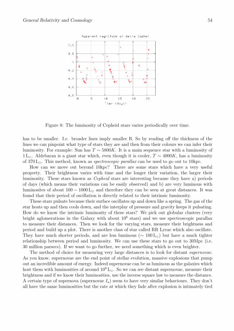
General Relativity and Cosmology 54
Figure 8: The luminosity of Cepheid stars varies periodically over time.
has to be smaller. I.e. broader lines imply smaller R. So by reading off the thickness of thelines we can pinpoint what type of stars they are and then from their colours we can infer theirluminosity. For example: Sun has T ∼ 5800K. It is a main sequence star with a luminosity of1 L⊙. Aldebaran is a giant star which, even though it is cooler, T ∼ 4000K, has a luminosityof 370 L⊙. This method, known as spectroscopic parallax can be used to go out to 10kpc.
How can we move out beyond 10kpc? There are some stars which have a very usefulproperty. Their brightness varies with time and the longer their variation, the larger theirluminosity. These stars known as Cepheid stars are interesting because they have a) periodsof days (which means their variations can be easily observed) and b) are very luminous withluminosites of about 100 − 1000 L⊙ and therefore they can be seen at great distances. It wasfound that their period of oscillation is directly related to their intrinsic luminosity.
These stars pulsate because their surface oscillates up and down like a spring. The gas of thestar heats up and then cools down, and the interplay of pressure and gravity keeps it pulsating.How do we know the intrinsic luminosity of these stars? We pick out globular clusters (verybright aglomerations in the Galaxy with about 106 stars) and we use spectroscopic parallaxto measure their distances. Then we look for the varying stars, measure their brightness andperiod and build up a plot. There is another class of star called RR Lyrae which also oscillate.They have much shorter periods, and are less luminous (∼ 100 L⊙) but have a much tighterrelationship between period and luminosity. We can use these stars to go out to 30Mpc (i.e.30 million parsecs). If we want to go further, we need something which is even brighter.
The method of choice for measuring very large distances is to look for distant supernovae.As you know, supernovae are the end point of stellar evolution, massive explosions that pumpout an incredible amount of energy. Indeed supernovae can be as luminous as the galaxies whichhost them with luminosities of around 109 L⊙. So we can see distant supernovae, measure theirbrightness and if we know their luminosities, use the inverse square law to measure the distance.A certain type of supernova (supernovae Ia) seem to have very similar behaviours. They don’tall have the same luminosities but the rate at which they fade after explosion is intimately tied
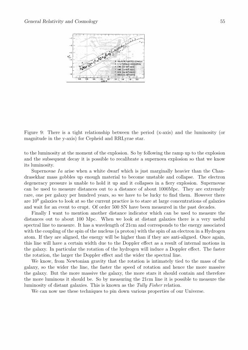
General Relativity and Cosmology 55
Figure 9: There is a tight relationship between the period (x-axis) and the luminosity (ormagnitude in the y-axis) for Cepheid and RRLyrae star.
to the luminosity at the moment of the explosion. So by following the ramp up to the explosionand the subsequent decay it is possible to recalibrate a supernova explosion so that we knowits luminosity.
Supernovae Ia arise when a white dwarf which is just marginally heavier than the Chan-drasekhar mass gobbles up enough material to become unstable and collapse. The electrondegeneracy pressure is unable to hold it up and it collapses in a fiery explosion. Supernovaecan be used to measure distances out to a distance of about 1000Mpc. They are extremelyrare, one per galaxy per hundred years, so we have to be lucky to find them. However thereare 109 galaxies to look at so the current practice is to stare at large concentrations of galaxiesand wait for an event to erupt. Of order 500 SN have been measured in the past decades.
Finally I want to mention another distance indicator which can be used to measure thedistances out to about 100 Mpc. When we look at distant galaxies there is a very usefulspectral line to measure. It has a wavelength of 21cm and corresponds to the energy associatedwith the coupling of the spin of the nucleus (a proton) with the spin of an electron in a Hydrogenatom. If they are aligned, the energy will be higher than if they are anti-aligned. Once again,this line will have a certain width due to the Doppler effect as a result of internal motions inthe galaxy. In particular the rotation of the hydrogen will induce a Doppler effect. The fasterthe rotation, the larger the Doppler effect and the wider the spectral line.
We know, from Newtonian gravity that the rotation is intimately tied to the mass of thegalaxy, so the wider the line, the faster the speed of rotation and hence the more massivethe galaxy. But the more massive the galaxy, the more stars it should contain and thereforethe more luminous it should be. So by measuring the 21cm line it is possible to measure theluminosity of distant galaxies. This is known as the Tully Fisher relation.
We can now use these techniques to pin down various properties of our Universe.
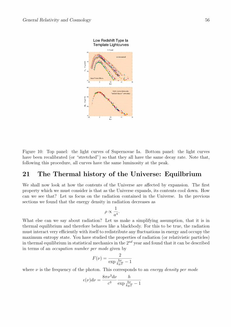
General Relativity and Cosmology 56
Figure 10: Top panel: the light curves of Supernovae Ia. Bottom panel: the light curveshave been recalibrated (or “stretched”) so that they all have the same decay rate. Note that,following this procedure, all curves have the same luminosity at the peak.
21 The Thermal history of the Universe: Equilbrium
We shall now look at how the contents of the Universe are affected by expansion. The firstproperty which we must consider is that as the Universe expands, its contents cool down. Howcan we see that? Let us focus on the radiation contained in the Universe. In the previoussections we found that the energy density in radiation decreases as
ρ ∝ 1
a4.
What else can we say about radiation? Let us make a simplifying assumption, that it is inthermal equilibrium and therefore behaves like a blackbody. For this to be true, the radiationmust interact very efficiently with itself to redistribute any fluctuations in energy and occupy themaximum entropy state. You have studied the properties of radiation (or relativistic particles)in thermal equilibrium in statistical mechanics in the 2nd year and found that it can be describedin terms of an occupation number per mode given by
F (ν) =2
exp hνkBT
− 1
where ν is the frequency of the photon. This corresponds to an energy density per mode
ǫ(ν)dν =8πν3dν
c3h
exp hνkBT
− 1
General Relativity and Cosmology 57
If we integrate over all frequencies we have that the energy density in photons is:
ργ =π2
15(kBT )
(
kBT
hc
)3
. (24)
We have therefore that ργ ∝ T 4. Hence if radiation is in thermal equilibrium we have that
T ∝ 1
a
Is this the temperature of the Universe? Two ingredients are necessary. First of all, everythingelse has to feel that temperature which means they have to interact (even if only indirectly)with the photons. For example the scattering off photons of electrons and positrons is throughthe emission and absorption of photons. And once again, at sufficiently high temperatures,everything interacts quite strongly.
Another essential ingredient is that the radiation must dominate over the remaining formsof matter in the Universe. We have to be careful with this because we know that differenttypes of energy will evolve in different ways as the Universe expands. For example we havethat the energy density of dust (or non-relativistic matter) evolves as ρNR ∝ a−3 as comparedto ργ ∝ a−4 so even if ργ was dominant at early times it may be negligible today. Howeverwe also know that the number density of photons, nγ ∝ a−3 as does the number density ofnon-relativistic particles, nNR ∝ a−3. If we add up all the non-relativisitic particle in the formof neutrons and protons (which we call baryons), we find that number density of baryons, nB
is very small compared to the number density of photons. In fact we can define the baryon toentropy ratio, ηB:
ηB =nB
nγ
≃ 10−10
As we can see there are many more photons in the Universe than particles like protons andneutrons. So it is safe to say that the temperature of the photons sets the temperature of theUniverse.
We can think of the Universe as a gigantic heat bath which is cooling with time. Thetemperature decreases as the inverse of the scale factor. To study the evolution of matterin the Universe we must now use statistical mechanics to follow the evolution of the variouscomponents as the temperature decreases. Let us start off with an ideal gas of bosons orfermions. Its occupation number per mode (now labeled in terms of momentum p) is
F (p) =g
exp(
E−µkBT
)
± 1
where g is the degeneracy factor, E =√p2c2 +M2c4 is the energy, µ is the chemical poten-
tial and + (-) corresponds to the Fermi-Dirac (Bose-Einstein) distribution. We can use thisexpression to calculate some macroscopic quantities such as the number density
n =g
h3
∫ d3p
exp(
E−µkBT
)
± 1
General Relativity and Cosmology 58
the energy density
ρc2 =g
h3
∫ E(p)d3p
exp(
E−µkBT
)
± 1
and the pressure
P =g
h3
∫ p2c2
3E
d3p
exp(
E−µT
)
± 1
It is instructive to consider two limits. First of all let us take the case where the tempera-ture of the Universe corresponds to energies which are much larger than the rest mass of theindividual particles, i.e. kBT ≫ Mc2 and let us take µ ≃ 0. We then have that the numberdensity obeys
n =ζ(3)
π2g
(
kBT
hc
)3
(B.E.)
n =3ζ(3)
4π2g
(
kBT
hc
)3
(F.D.)
where ζ(3) ≃ 1.2 comes from doing the integral. The energy density is given by
ρc2 = gπ2
30(kBT )
(
kBT
hc
)3
(B.E.)
ρc2 =7
8gπ2
30(kBT )
(
kBT
hc
)3
(F.D.)
and pressure satisfies P = ρc2/3. As you can see these are the properties of a radiation. Inother words, even massive particles will behave like radiation at sufficiently high temperatures.At low temperatures we have kBT ≪ Mc2 and for both fermions and bosons the macroscopicquantities are given by:
n = g(
2π
h2
)
3
2
(MkBT )3/2 exp(−Mc2
kBT)
ρc2 = Mc2n
P = nkBT ≪ Mc2n = ρ.
This last expression tells us that the pressure is negligible as it should be for non-relativisticmatter.
This calculation has already given us an insight into how matter evolves during expansion.At sufficiently early times it all looks like radiation. As it cools down and the temperature fallsbelow mass thresholds, the number of particles behaving relativistically decreases until whenwe get to today, there are effectively only three type of particles which behave relativistically:the three types of neutrinos. We denote the effective number of relativistic degrees of freedomby g∗ and the energy density in relativistic degrees of freedom is given by
ρ = g∗π2
30(kBT )
(
kBT
hc
)3
General Relativity and Cosmology 59
22 The Thermal history of the Universe: The Cosmic
Microwave Background
Until now we have considered things evolving passively, subjected to the expansion of theUniverse. But we know that the interactions between different components of matter can be farmore complex. Let us focus on the realm of chemistry, in particular on the interaction betweenone electron and one proton. From atomic physics and quantum mechanics you already knowthat an electron and a proton may bind together to form a Hydrogen atom. To tear the electronaway we need an energy of about 13.6eV . But imagine now that the universe is sufficiently hotthat there are particles zipping around that can knock the electron out of the atom. We canimagine that at high temperatures it will be very difficult to keep electrons and protons boundtogether. If the temperature of the Universe is such that T ≃ 13.6eV then we can imagine thatthere will be a transition between ionized and neutral hydrogen.
We can work this out in more detail (although not completely accurately) if we assume thatthis transition occurs in thermal equilibrium throughout. Let us go through the steps that leadto the Saha equation. Assume we have an equilibrium distribution of protons, electrons andhydrogen atoms. Let np, ne and nH be their number densities. In thermal equilibrium (withT ≪ M) we have that the number densities are given by
ni = gi
(
2π
h2
)
3
2
(MikBT )3
2 expµi −Mic
2
kBT
where i = p, n,H. In chemical equlibrium we have that
µp + µe = µH
so that
nH = gH
(
2π
h2
)
3
2
(MHkBT )3
2 exp−MHc
2
kBTexp
(µp + µe)
kBT
We can use the expressions for np and ne to eliminate the chemical potentials and obtain:
nH = nenpgHgpge
(
2π
h2
)− 3
2
(MHkBT )3
2 (MpkBT )− 3
2 (MekBT )− 3
2 exp−MHc
2 +Mpc2 +Mec
2
kBT
There are a series of simplifications we can now consider: i) Mp ≃ MH , ii) the binding energyis B ≡ −MHc
2 +Mpc2 +Mec
2 = 13.6eV , iii) nB = np + nH iv) ne = np and finally gp = ge = 2and gH = 4. So we end up with
nH = n2p(MekBT )
− 3
2
(
2π
h2
)− 3
2
expB
kBT
We can go further and define an ionization fraction X ≡ np
nB. Quite clearly we have X is 1 if
the Universe is completely ionized and 0 if it is neutral. Using the definition of the baryon toentropy fraction we have
1−X = X2ηBnγ
(
2π
h2
)− 3
2
(MekBT )− 3
2 expB
kBT(25)
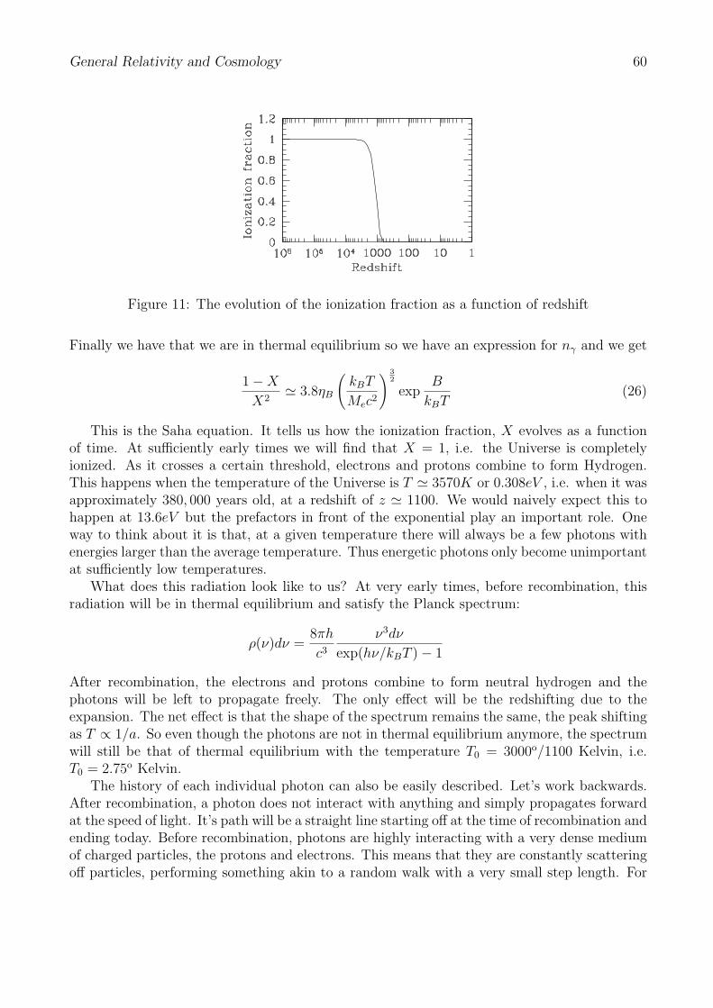
General Relativity and Cosmology 60
Figure 11: The evolution of the ionization fraction as a function of redshift
Finally we have that we are in thermal equilibrium so we have an expression for nγ and we get
1−X
X2≃ 3.8ηB
(
kBT
Mec2
)3
2
expB
kBT(26)
This is the Saha equation. It tells us how the ionization fraction, X evolves as a functionof time. At sufficiently early times we will find that X = 1, i.e. the Universe is completelyionized. As it crosses a certain threshold, electrons and protons combine to form Hydrogen.This happens when the temperature of the Universe is T ≃ 3570K or 0.308eV , i.e. when it wasapproximately 380, 000 years old, at a redshift of z ≃ 1100. We would naively expect this tohappen at 13.6eV but the prefactors in front of the exponential play an important role. Oneway to think about it is that, at a given temperature there will always be a few photons withenergies larger than the average temperature. Thus energetic photons only become unimportantat sufficiently low temperatures.
What does this radiation look like to us? At very early times, before recombination, thisradiation will be in thermal equilibrium and satisfy the Planck spectrum:
ρ(ν)dν =8πh
c3ν3dν
exp(hν/kBT )− 1
After recombination, the electrons and protons combine to form neutral hydrogen and thephotons will be left to propagate freely. The only effect will be the redshifting due to theexpansion. The net effect is that the shape of the spectrum remains the same, the peak shiftingas T ∝ 1/a. So even though the photons are not in thermal equilibrium anymore, the spectrumwill still be that of thermal equilibrium with the temperature T0 = 3000o/1100 Kelvin, i.e.T0 = 2.75o Kelvin.
The history of each individual photon can also be easily described. Let’s work backwards.After recombination, a photon does not interact with anything and simply propagates forwardat the speed of light. It’s path will be a straight line starting off at the time of recombination andending today. Before recombination, photons are highly interacting with a very dense mediumof charged particles, the protons and electrons. This means that they are constantly scatteringoff particles, performing something akin to a random walk with a very small step length. For
General Relativity and Cosmology 61
all intents and purposes, they are glued to the spot unable to move. So one can think of sucha photon’s history as starting off stuck at some point in space and, at recombination, beingreleased to propogate forward until now.
We can take this even further. If we look from a specific observing point (such as the Earthor a satellite), we will be receiving photons from all directions that have been travelling in astraight line since the Universe recombined. All these straight lines will have started off at thesame time and at the same distance from us-i.e. they will have started off from the surface ofa sphere. This surface, known as the surface of last scattering is what we see when we look atthe relic radiation. It is very much like a photograph of the Universe when it was 380,000 yearsold.
23 The Thermal history of the Universe: out of equili-
birium and Big Bang Nucleosynthesis
We have assumed that the Universe is in thermal equilibrium throughout this process. We havecome up with an expression for the ionization fraction which is not completely accurate butqualitatively has the correct behaviour. There is another situation where assuming thermalequilibrium will not only give us the wrong quantitative but also the wrong qualitative result.We shall now look at what happens when the temperature of the Universe is kBT ≃ 1MeV .This corresponds to the energy where nuclear processes play an important role.
The particles we will consider are protons (p) and neutrons (n). These particles will combineto form the nuclei of the elements. For example
1p → Hydrogen nucleus
1p+ 1n → Deuterium nucleus
1p+ 2n → Tritium nucleus
2p+ 1n → Helium 3 nucleus
2p+ 2n → Helium 4 nucleus (27)
The binding energy of each nucleus will be the difference between the mass of the nucleus andthe sum of masses of the protons and neutrons that form it. For example the binding energy ofDeuterium is BD = 2.22MeV . The neutrons and protons can convert into each other throughthe weak interactions:
p+ νe → n+ e+
p+ e− → n+ ν
n → p+ e− + ν
(28)
Let us start with an equilibrium approach. We can try to work out the abundance of lightelements of the Universe using the same rationale we used above. Once again we have
ni = gi
(
2π
h2
)
3
2
(MikBT )3
2 expµi −Mic
2
kBT
General Relativity and Cosmology 62
Let us assume thermal equilibrium (µn = µp). We have that
neqn
neqp
= exp(
− Q
kBT
)
(29)
where Q is the energy due to the mass difference between the neutron and the proton, Q =1.293MeV . We can see that at high temperatures there are as many protons as neutrons. Butas T falls below Q the mass difference becomes important and the neutrons dwindle away. Ifthis were the correct way of calculating the abundance of neutrons we would find that as theUniverse cools, all the neutrons would dissapear. No neutrons would be left.
To get an accurate estimate we must go beyond the equilibrium approximation. We canstep back a bit and think about what is actually going on when protons and neutrons areinterconverting into each other. The reaction can be characterised in terms of a reaction rate,Γ which has units of s−1. The reaction must compete against the expansion of the universewhich itself can be described in terms of a “rate”: the expansion rate H which has units of s−1.The relative sizes of Γ and H dictate how important the reactions are in keeping the neutronsand protons equilibrated.
One can write down a Boltzmann equation for the comoving neutron number (the numberof neutrons in a box in comoving units):
d lnNn
d ln a= − Γ
H
[
1−(
N eqn
Nn
)2]
Where N eqn = a3neq
n is the equilibrium expression given above. If Γ ≫ H we have that Nn →N eq
n , i.e. the neutron number density will be pushed to its equilibrium value. In that regimewe will have the ratio of neutrons as given by 29. If, however, Γ ≪ H, the expansion of theuniverse will win out and inhibit the depletion or creation of neutrons through that reaction.The equation is then approximately given by
d lnNn
d ln a≃ 0
i.e. the neutron comoving number is frozen (and the number density will decay as a−3). Thetransition from one regime to the other will occur when Γ ∼ H and it will depend on howthe reaction rate depends on temperature and masses. It turns out that for this reaction, thetemperature at which reactions “freeze out” is kBTf ≃ 0.7 − 0.8MeV . The relative numberdensity of neutrons to protons will be frozen in at
neqn
neqp
≃ 1
6
In fact the neutron decay rate plays a role as well to further decrease the fraction of neutronsso that we in fact get nn/np → 1
7. We can use a very simple argument to find the fraction of
Helium 4 in the Universe. We start off with 7/8 in protons and 1/8 in neutrons. Let us assumethat the neutrons are used to make Helium atoms. We then need to pair up the 1/8 with 1/8protons, reducing the number of unpaired protons to 6/8 ≃ 75%. So we roughly expect to haveabout 25% of the mass in Helium and 75% in Hydrogen. A more accurate calculation gives a
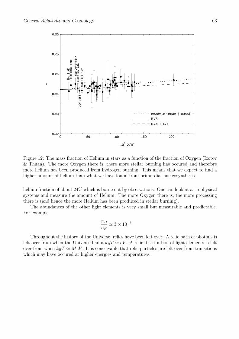
General Relativity and Cosmology 63
Figure 12: The mass fraction of Helium in stars as a function of the fraction of Oxygen (Izotov& Thuan). The more Oxygen there is, there more stellar burning has occured and thereforemore helium has been produced from hydrogen burning. This means that we expect to find ahigher amount of helium than what we have found from primordial nucleosynthesis
helium fraction of about 24% which is borne out by observations. One can look at astrophysicalsystems and measure the amount of Helium. The more Oxygen there is, the more processingthere is (and hence the more Helium has been produced in stellar burning).
The abundances of the other light elements is very small but measurable and predictable.For example
nD
nH
≃ 3× 10⁻⁵
Throughout the history of the Universe, relics have been left over. A relic bath of photons isleft over from when the Universe had a kBT ≃ eV . A relic distribution of light elements is leftover from when kBT ≃ MeV . It is conceivable that relic particles are left over from transitionswhich may have occured at higher energies and temperatures.