Embed Size (px)
Citation preview
1
General Physics Virtual Lab Thermodynamics and Molecular Physics
2021
1. INTERNAL ENERGY AND MECHANICAL WORK
The experiment is conducted to investigate the increase in the internal energy of an aluminum (or copper) body caused by mechanical work. The cylindrical body is rotated about its axis by means of a hand-operated crank. A cord running over the curved surface provides the friction to heat the body. The frictional force F corresponds to the weight of a mass that is suspended from the end of the friction cord. The work performed against friction during n revolutions of the body is
(1.1)
where d – cylindrical body diameter. During the n revolutions, the frictional work raises the temperature of the body from
the initial value T0 to the final value Tn. At the same time the internal energy is increased by
(1.2)
where m – body mass, cAl – specific heat capacity of aluminium. To avoid pure heat exchange with the environment as much as possible, the body is
cooled before starting the measurement to an initial temperature T0, which is only slightly below room temperature.
The transformation of internal energy corresponds to the work done:
(1.3)
From Equations 1.2 and 1.3:
(1.4)
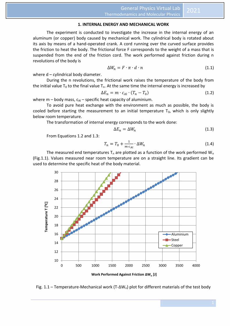
The measured end temperatures Tn are plotted as a function of the work performed Wn (Fig.1.1). Values measured near room temperature are on a straight line. Its gradient can be used to determine the specific heat of the body material.
Fig. 1.1 – Temperature-Mechanical work (T-ΔWn) plot for different materials of the test body
10
12
14
16
18
20
22
24
26
28
30
0 500 1000 1500 2000 2500 3000 3500 4000
Tem
pe
ratu
re T
[0 C
]
Work Performed Against Friction ΔWn [J]
Aluminium
Steel
Copper
2
General Physics Virtual Lab Thermodynamics and Molecular Physics
2021
2. INTERNAL ENERGY AND ELECTRICAL WORK
This laboratory work demonstrates how the internal energy of copper and aluminum bodies is increased by the work of electricity. This is proportional to the applied voltage U, the flowing current I and the measurement time t:
(2.1) The work of the electric current causes the body temperature to rise from the initial
value T0 to the final value Tn. Internal energy increases by the value:
(2.2)
where m – body mass, c – specific heat capacity of the body material. To minimize the transfer of heat to the environment as much as possible, the body is first cooled to an initial temperature T0 before any measurements are taken. It should be only slightly below the ambient temperature. Under such conditions, the change in internal energy should be equal to the work done, which means the following:
(2.3)
The temperature sensor is used to measure the temperature T by measuring its resistance, which depends on the temperature:
(2.4)
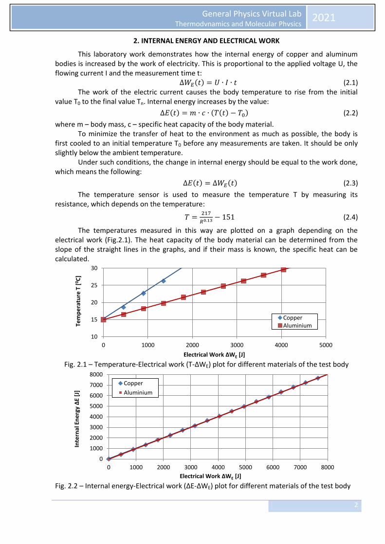
The temperatures measured in this way are plotted on a graph depending on the electrical work (Fig.2.1). The heat capacity of the body material can be determined from the slope of the straight lines in the graphs, and if their mass is known, the specific heat can be calculated.
Fig. 2.1 – Temperature-Electrical work (T-ΔWE) plot for different materials of the test body
Fig. 2.2 – Internal energy-Electrical work (ΔE-ΔWE) plot for different materials of the test body
10
15
20
25
30
0 1000 2000 3000 4000 5000
Tem
pe
ratu
re T
[0 C
]
Electrical Work ΔWE [J]
Copper Aluminium
0
1000
2000
3000
4000
5000
6000
7000
8000
0 1000 2000 3000 4000 5000 6000 7000 8000
Inte
rnal
En
erg
y Δ
E [J
]
Electrical Work ΔWE [J]
Copper
Aluminium
3
General Physics Virtual Lab Thermodynamics and Molecular Physics
2021
3. BOYLE'S LAW
The law discovered by Boyle and Mariotte
(3.1)
and is a special case of a more general law applicable to all ideal gases. This general law describes the relationship between pressure p, volume V, temperature T relative to absolute zero, and the amount of gas n:
(3.2)
where R = 8.314 J/(mol·K) – universal gas constant. A special case 3.1 is derived from the general equation 3.2, provided that the temperature T and the amount of gas n do not change.
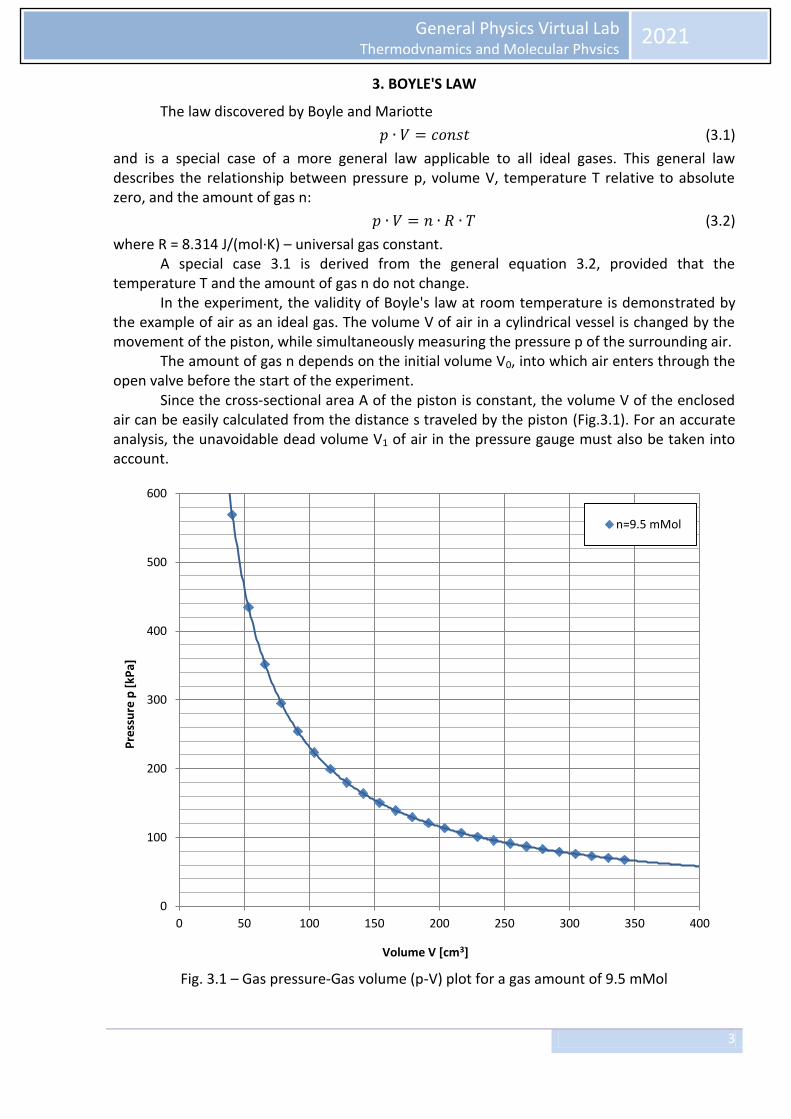
In the experiment, the validity of Boyle's law at room temperature is demonstrated by the example of air as an ideal gas. The volume V of air in a cylindrical vessel is changed by the movement of the piston, while simultaneously measuring the pressure p of the surrounding air.
The amount of gas n depends on the initial volume V0, into which air enters through the open valve before the start of the experiment.
Since the cross-sectional area A of the piston is constant, the volume V of the enclosed air can be easily calculated from the distance s traveled by the piston (Fig.3.1). For an accurate analysis, the unavoidable dead volume V1 of air in the pressure gauge must also be taken into account.
Fig. 3.1 – Gas pressure-Gas volume (p-V) plot for a gas amount of 9.5 mMol
0
100
200
300
400
500
600
0 50 100 150 200 250 300 350 400
Pre
ssu
re p
[kP
a]
Volume V [cm3]
n=9.5 mMol
4
General Physics Virtual Lab Thermodynamics and Molecular Physics
2021
4. AMONTONS' LAW
The law discovered by Amontons
(4.1)
is a special case of a more general law applicable to all ideal gases. This general law describes the relationship between pressure p, volume V, temperature T relative to absolute zero, and the amount of gas n:
(4.2)
where R = 8.314 J/(mol·K) – universal gas constant. A special case 4.1 is derived from the general equation 4.2, provided that the
temperature T and the amount of gas n do not change. In laboratory work, the validity of Amontons' law is demonstrated using air as an ideal
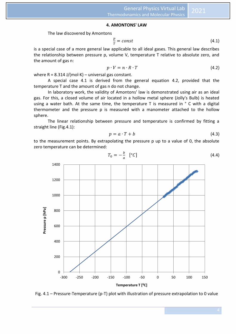
gas. For this, a closed volume of air located in a hollow metal sphere (Jolly's Bulb) is heated using a water bath. At the same time, the temperature T is measured in ° C with a digital thermometer and the pressure p is measured with a manometer attached to the hollow sphere.
The linear relationship between pressure and temperature is confirmed by fitting a straight line (Fig.4.1):
(4.3)
to the measurement points. By extrapolating the pressure p up to a value of 0, the absolute zero temperature can be determined:
(4.4)
Fig. 4.1 – Pressure-Temperature (p-T) plot with illustration of pressure extrapolation to 0 value
0
200
400
600
800
1000
1200
1400
-300 -250 -200 -150 -100 -50 0 50 100 150
Pre
ssu
re p
[h
Pa]
Temperature T [0C]

5
General Physics Virtual Lab Thermodynamics and Molecular Physics
2021
5. ADIABATIC INDEX OF AIR
Since there is no heat exchange with the environment, vibrations of the piston in the glass tube are associated with adiabatic changes in state. The following equation describes the relationship between pressure p and volume V of enclosed air:
(5.1)
The adiabatic index γ is the ratio between the specific heat capacity at constant pressure CP and constant volume CV:
(5.2)
From equation 5.1, the following relationship can be derived for changes in pressure and volume Δp and ΔV:
(5.3)
By substituting the inner cross-sectional area A of the tube, the restoring force ΔF can be calculated from the pressure change. Likewise, the deviation of the piston from its equilibrium position can be determined from the change in volume.
Therefore
(5.4)
The equation of motion for the oscillating piston is
(5.5)
where m – piston mass. Solutions to this classical equation of motion for simple harmonic oscillators are
oscillations with the period:
(5.6)
From this, the adiabatic index can be calculated as long as all the other variables are known. In this lab work, a precision glass tube of small cross-section A is placed vertically into an opening through a large volume glass vessel stopper V (Mariotte bottle), and a corresponding aluminum piston of known mass m can slide up and down inside the tube. The aluminum piston performs a simple harmonic movement on an air cushion formed by a closed volume. The adiabatic index can be calculated from the oscillation period of the piston. The equilibrium volume V corresponds to the volume of the gas vessel, since that of the tube is small enough to be disregarded.
(5.7)
The equilibrium pressure p is obtained from the external air pressure p0 and the pressure exerted by the aluminum piston on the enclosed air in its rest state:
(5.8)
The expected result is therefore γ=7/5=1.4, since air predominantly consists of diatomic molecules with 5 degrees of freedom for the absorption of heat energy.
6
General Physics Virtual Lab Thermodynamics and Molecular Physics
2021
6. REAL GASES AND CRITICAL POINT
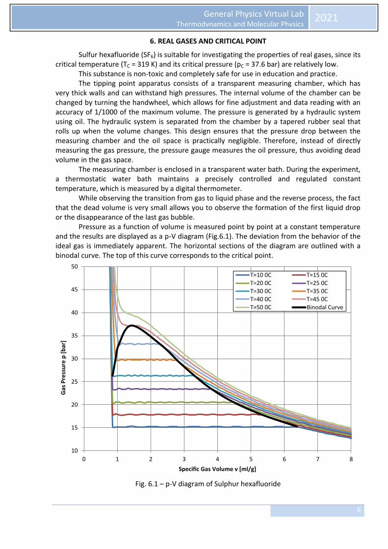
Sulfur hexafluoride (SF6) is suitable for investigating the properties of real gases, since its critical temperature (TC = 319 K) and its critical pressure (pC = 37.6 bar) are relatively low.
This substance is non-toxic and completely safe for use in education and practice. The tipping point apparatus consists of a transparent measuring chamber, which has
very thick walls and can withstand high pressures. The internal volume of the chamber can be changed by turning the handwheel, which allows for fine adjustment and data reading with an accuracy of 1/1000 of the maximum volume. The pressure is generated by a hydraulic system using oil. The hydraulic system is separated from the chamber by a tapered rubber seal that rolls up when the volume changes. This design ensures that the pressure drop between the measuring chamber and the oil space is practically negligible. Therefore, instead of directly measuring the gas pressure, the pressure gauge measures the oil pressure, thus avoiding dead volume in the gas space.
The measuring chamber is enclosed in a transparent water bath. During the experiment, a thermostatic water bath maintains a precisely controlled and regulated constant temperature, which is measured by a digital thermometer.
While observing the transition from gas to liquid phase and the reverse process, the fact that the dead volume is very small allows you to observe the formation of the first liquid drop or the disappearance of the last gas bubble.
Pressure as a function of volume is measured point by point at a constant temperature and the results are displayed as a p-V diagram (Fig.6.1). The deviation from the behavior of the ideal gas is immediately apparent. The horizontal sections of the diagram are outlined with a binodal curve. The top of this curve corresponds to the critical point.
Fig. 6.1 – p-V diagram of Sulphur hexafluoride
10
15
20
25
30
35
40
45
50
0 1 2 3 4 5 6 7 8
Gas
Pre
ssu
re p
[b
ar]
Specific Gas Volume v [ml/g]
T=10 0C T=15 0C T=20 0C T=25 0C T=30 0C T=35 0C T=40 0C T=45 0C T=50 0C Binodal Curve
7
General Physics Virtual Lab Thermodynamics and Molecular Physics
2021
7. LESLIE CUBE
The radiated intensity of the body surface is described by the emissivity E. The absorption capacity A is the ratio between the intensity of the absorbed and incident radiation. The absorption capacity increases with emissivity. More specifically, according to Kirchhoff's law, the relationship between emissivity and absorbance is the same for all bodies at a given temperature and corresponds to the ESB emissivity of a black body at this temperature:
(7.1)
where σ – Stefan-Boltzmann constant, T – temperature in Kelvin. The degree to which the absorbency depends on temperature is usually negligible.
Therefore, the emissivity of a body can be described by (7.2)
If the body has the same temperature T0 as its environment, the intensity of the heat emitted by the body into the environment is equal to the intensity of the heat that it absorbs from them:
(7.3)
If the body’s temperature is higher, the intensity of the radiation absorbed from the surroundings does not change as long as the ambient temperature remains constant. The energy radiated by a body per unit of surface and time and measurable by means of a radiation detector is
(7.4)
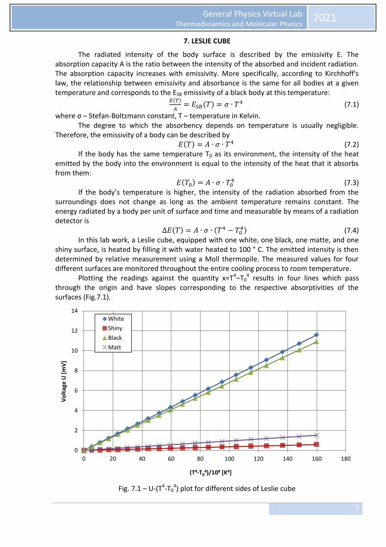
In this lab work, a Leslie cube, equipped with one white, one black, one matte, and one shiny surface, is heated by filling it with water heated to 100 ° C. The emitted intensity is then determined by relative measurement using a Moll thermopile. The measured values for four different surfaces are monitored throughout the entire cooling process to room temperature.
Plotting the readings against the quantity x=T4–T04 results in four lines which pass
through the origin and have slopes corresponding to the respective absorptivities of the surfaces (Fig.7.1).
Fig. 7.1 – U-(T4-T0
4) plot for different sides of Leslie cube
0
2
4
6
8
10
12
14
0 20 40 60 80 100 120 140 160 180
Vo
ltag
e U
[m
V]
(T4-T04)/108 [K4]
White
Shiny
Black
Matt
8
General Physics Virtual Lab Thermodynamics and Molecular Physics
2021
8. HEAT CONDUCTION
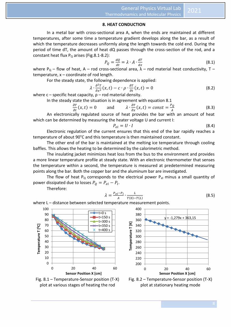
In a metal bar with cross-sectional area A, when the ends are maintained at different temperatures, after some time a temperature gradient develops along the bar, as a result of which the temperature decreases uniformly along the length towards the cold end. During the period of time dT, the amount of heat dQ passes through the cross-section of the rod, and a constant heat flux PQ arises (Fig.8.1-8.2):
(8.1)
where PQ – flow of heat, A – rod cross-sectional area, λ – rod material heat conductivity, T – temperature, x – coordinate of rod length.
For the steady state, the following dependence is applied:
(8.2)
where c – specific heat capacity, ρ – rod material density. In the steady state the situation is in agreement with equation 8.1
(8.3)
An electronically regulated source of heat provides the bar with an amount of heat which can be determined by measuring the heater voltage U and current I:
(8.4) Electronic regulation of the current ensures that this end of the bar rapidly reaches a
temperature of about 90°C and this temperature is then maintained constant. The other end of the bar is maintained at the melting ice temperature through cooling
baffles. This allows the heating to be determined by the calorimetric method. The insulating jacket minimizes heat loss from the bus to the environment and provides
a more linear temperature profile at steady state. With an electronic thermometer that senses the temperature within a second, the temperature is measured at predetermined measuring points along the bar. Both the copper bar and the aluminum bar are investigated.
The flow of heat PQ corresponds to the electrical power Pel minus a small quantity of power dissipated due to losses .
Therefore:
(8.5)
where L – distance between selected temperature measurement points.
Fig. 8.1 – Temperature-Sensor position (T-X)
plot at various stages of heating the rod
Fig. 8.2 – Temperature-Sensor position (T-X)
plot at stationary heating mode
0
10
20
30
40
50
60
70
80
90
100
0 20 40 60
Tem
pe
ratu
re T
[0 C
]
Sensor Position X [cm]
t=0 s t=150 s t=300 s t=350 s t=400 s
y = -1,279x + 363,15
200
220
240
260
280
300
320
340
360
380
400
0 20 40 60
Tem
pe
ratu
re T
[K
]
Sensor Position X [cm]
9
General Physics Virtual Lab Thermodynamics and Molecular Physics
2021
9. THERMAL EXPANSION OF SOLID BODIES
The coefficient of linear expansion of material is defined as:
(9.1)
where L – rod length, T – temperature 0C. This coefficient depends strongly on the nature of the material and is usually less responsive to the temperature. This leads to the following equation:
(9.2)
where L0 - rod length in the absence of temperature change. If the temperature is not very high:
(9.3)
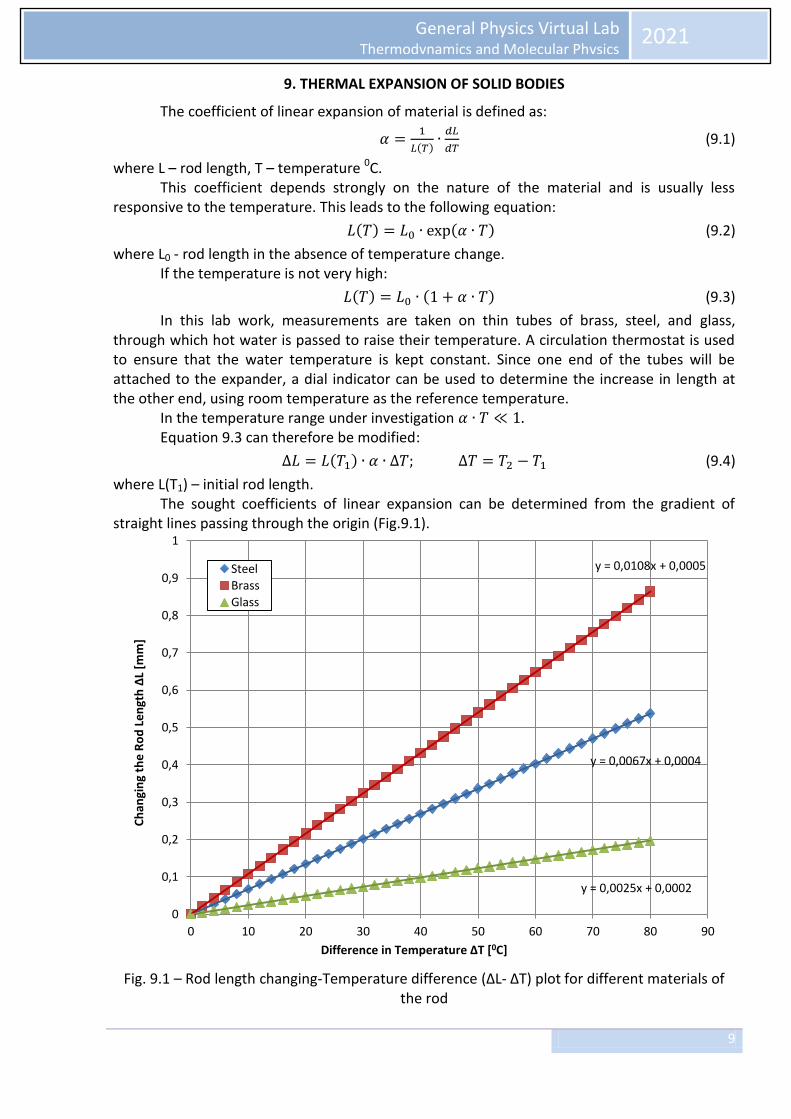
In this lab work, measurements are taken on thin tubes of brass, steel, and glass, through which hot water is passed to raise their temperature. A circulation thermostat is used to ensure that the water temperature is kept constant. Since one end of the tubes will be attached to the expander, a dial indicator can be used to determine the increase in length at the other end, using room temperature as the reference temperature. In the temperature range under investigation Equation 9.3 can therefore be modified:
(9.4)
where L(T1) – initial rod length. The sought coefficients of linear expansion can be determined from the gradient of straight lines passing through the origin (Fig.9.1).
Fig. 9.1 – Rod length changing-Temperature difference (ΔL- ΔT) plot for different materials of
the rod
y = 0,0067x + 0,0004
y = 0,0108x + 0,0005
y = 0,0025x + 0,0002
0
0,1
0,2
0,3
0,4
0,5
0,6
0,7
0,8
0,9
1
0 10 20 30 40 50 60 70 80 90
Ch
angi
ng
the
Ro
d L
en
gth
ΔL
[mm
]
Difference in Temperature ΔT [0C]
Steel
Brass
Glass
10
General Physics Virtual Lab Thermodynamics and Molecular Physics
2021
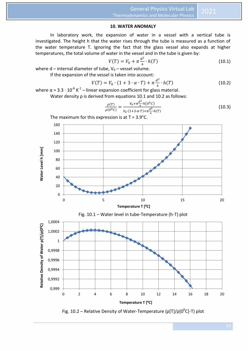
10. WATER ANOMALY
In laboratory work, the expansion of water in a vessel with a vertical tube is investigated. The height h that the water rises through the tube is measured as a function of the water temperature T. Ignoring the fact that the glass vessel also expands at higher temperatures, the total volume of water in the vessel and in the tube is given by:
(10.1)
where d – internal diameter of tube, V0 – vessel volume. If the expansion of the vessel is taken into account:
(10.2)
where α = 3.3 · 10-6 K-1 – linear expansion coefficient for glass material. Water density ρ is derived from equations 10.1 and 10.2 as follows:
(10.3)
The maximum for this expression is at T = 3.9°C.
Fig. 10.1 – Water level in tube-Temperature (h-T) plot
Fig. 10.2 – Relative Density of Water-Temperature (ρ[T]/ρ[00C]-T) plot
0
20
40
60
80
100
120
140
160
0 5 10 15 20
Wat
er
Leve
l h [
mm
]
Temperature T [0C]
0,999
0,9992
0,9994
0,9996
0,9998
1
1,0002
1,0004
0 2 4 6 8 10 12 14 16 18 20
Re
lati
ve D
en
sity
of
Wat
er ρ(T
)/ρ(0
0 C)
Temperature T [0C]

11
General Physics Virtual Lab Thermodynamics and Molecular Physics
2021
11. STIRLING ENGINE D
If the hot air motor is running without any mechanical load, it rotates at an idle speed that is limited by internal friction and depends on the amount of heat energy supplied. The Stirling engine cycle (Fig.11.1) includes the following steps.
Heating: heat is introduced when the piston is extended, pushing air into the heated area of the large cylinder. During this operation, the working piston is at its bottom dead center because the displacement piston is 90 ° ahead of the working piston. Expansion: the heated air expands and forces the working piston to retract. At the same time, mechanical work is transferred to the flywheel rod via the crankshaft. Cooling: while the working piston is in its top dead center position: the displacement piston retracts and air is displaced towards the top end of the large cylinder so that it cools. Compression: the cooled air is compressed by extending the working piston. The mechanical work required for this is provided by the flywheel stem. If we consider the internal friction constant, then the idle speed is proportional to the mechanical energy released by the Stirling engine in an unloaded state. If, in addition, the heater resistance is assumed constant, then the heating energy is proportional to the square of the heater voltage. Thus, in Fig. 11.2 the idling speed n of a Stirling engine (as a measure of the mechanical energy output) is presented as a function of the square of the heater voltage U (as a measure of the thermal energy input).
Fig. 11.1 – p-V diagram of Stirling Engine model D
Fig. 11.2 – No-load Speed-Voltage Square (n-U2) for Stirling Engine model D
98,5
99
99,5
100
100,5
101
101,5
102
102,5
103
103,5
104
330 332 334 336 338 340 342 344 346 348
Gas
Pre
ssu
re p
[kP
a]
Gas Volume v [cm3]
0
0,1
0,2
0,3
0,4
0,5
0,6
0,7
0,8
0,9
1
0 50 100 150 200 250
No
-lo
ad S
pe
ed
n [
1/s
]
Voltage Square U2 [V2]
12
General Physics Virtual Lab Thermodynamics and Molecular Physics
2021
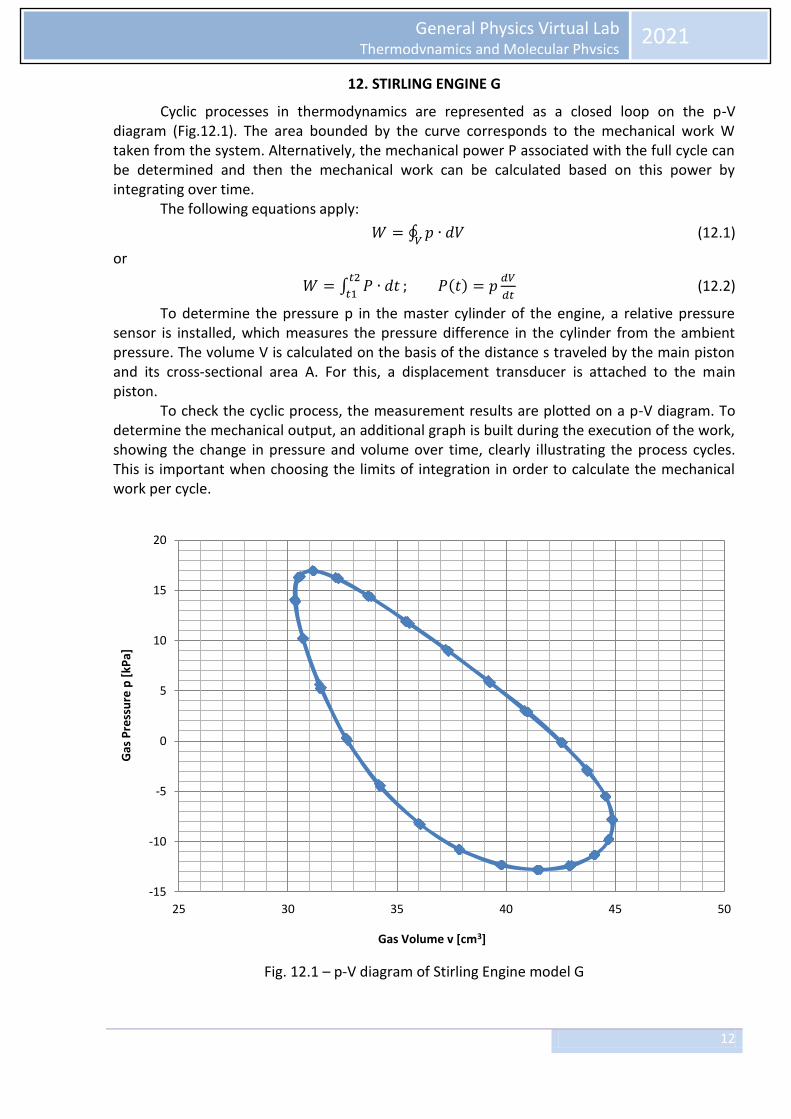
12. STIRLING ENGINE G
Cyclic processes in thermodynamics are represented as a closed loop on the p-V diagram (Fig.12.1). The area bounded by the curve corresponds to the mechanical work W taken from the system. Alternatively, the mechanical power P associated with the full cycle can be determined and then the mechanical work can be calculated based on this power by integrating over time.
The following equations apply:
(12.1)
or
(12.2)
To determine the pressure p in the master cylinder of the engine, a relative pressure sensor is installed, which measures the pressure difference in the cylinder from the ambient pressure. The volume V is calculated on the basis of the distance s traveled by the main piston and its cross-sectional area A. For this, a displacement transducer is attached to the main piston.
To check the cyclic process, the measurement results are plotted on a p-V diagram. To determine the mechanical output, an additional graph is built during the execution of the work, showing the change in pressure and volume over time, clearly illustrating the process cycles. This is important when choosing the limits of integration in order to calculate the mechanical work per cycle.
Fig. 12.1 – p-V diagram of Stirling Engine model G
-15
-10
-5
0
5
10
15
20
25 30 35 40 45 50
Gas
Pre
ssu
re p
[kP
a]
Gas Volume v [cm3]
13
General Physics Virtual Lab Thermodynamics and Molecular Physics
2021
13. HEAT PUMPS
The electric compression heat pump consists of a compressor driven by a motor, a condenser, an expansion valve and an evaporator. Its work is based on a cyclic process - a phase change, which the working medium inside the pump undergoes. Ideally, this process can be divided into four stages, including compression, liquefaction, depressurization, and evaporation.
For the compression part of the cycle, the gaseous working fluid is sucked in by the compressor and compressed without any change in entropy (s1=s2) from p1 to p2, while the medium is heated. Accordingly, the temperature rises from T1 to T2. The work of mechanical compression, produced per unit mass, is equal to Δw=h2–h1.
Inside the condenser, the working medium is significantly cooled and condensed. The heat released as a result (excess heat and latent heat of condensation) per unit mass is equal to Δq2=h2–h3. Raises the temperature of the surrounding water body.
The condensed medium reaches the outlet valve where the pressure is released (without any mechanical work). In this process, the temperature also decreases due to the work that must be done in opposition to the molecular forces of attraction inside the working fluid (Joule-Thomson effect). Enthalpy remains constant (h4=h3).
By absorbing the heat inside the evaporator, the working fluid is completely vaporized. This cools the surrounding tank. The heat absorbed by a unit of mass is equal to Δq1=h1–h4.
The Mollier diagram of the working fluid is often used to represent the cycle of a compression heat pump. This diagram shows the dependence of pressure p on the specific enthalpy h of the working fluid (enthalpy is a measure of the heat content of the working fluid and usually increases with increasing pressure and gas content).
Isotherms (T=const) and isentropes (S=const) are also indicated, as well as the relative mass fraction of the working fluid in the liquid phase. The working fluid is completely condensed to the left of the evaporation interface. The medium is present as superheated vapor to the right of the condensation interface and as a mixture of liquid and gas between the two lines. The two lines touch at a critical point.
To depict the system in a Mollier diagram, the ideal cycle described above can be determined by measuring the pressures p1 and p2, respectively, before and after the expansion valve, and the temperatures T1 and T3, respectively, upstream of the compressor and expansion valve.
The theoretical efficiency for an ideal cyclic process can be calculated from the specific enthalpies h1, h2 and h3 read from the Mollier diagram:
(13.1)
Determination of the enthalpies h2 and h3 of the ideal cyclic process and the amount of heat ΔQ2 supplied to the hot water tank during the time interval Δt allows us to estimate the mass flow rate of the working fluid.
(13.2)
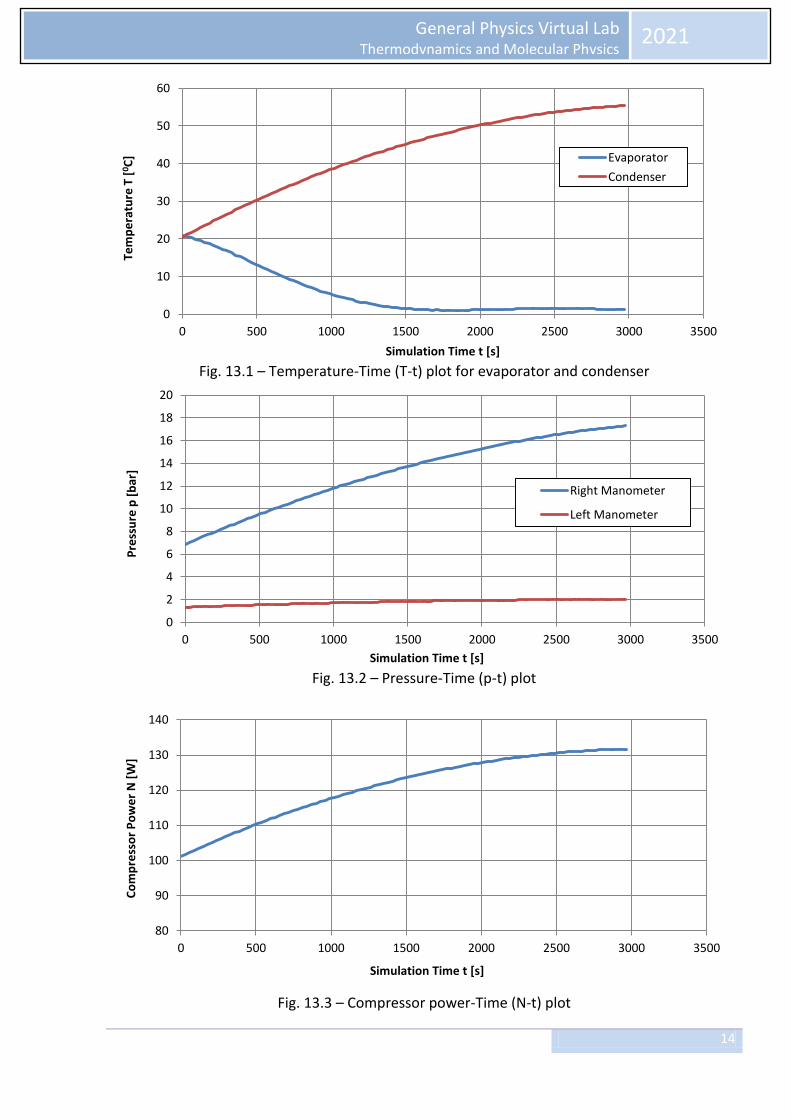
A vector Mollier diagram is attached to these guidelines. Figures 13.1-13.3 show the main experimental dependences of temperature, pressure and compressor power versus time.
14
General Physics Virtual Lab Thermodynamics and Molecular Physics
2021
Fig. 13.1 – Temperature-Time (T-t) plot for evaporator and condenser
Fig. 13.2 – Pressure-Time (p-t) plot
Fig. 13.3 – Compressor power-Time (N-t) plot
0
10
20
30
40
50
60
0 500 1000 1500 2000 2500 3000 3500
Tem
pe
ratu
re T
[0 C
]
Simulation Time t [s]
Evaporator
Condenser
0
2
4
6
8
10
12
14
16
18
20
0 500 1000 1500 2000 2500 3000 3500
Pre
ssu
re p
[b
ar]
Simulation Time t [s]
Right Manometer
Left Manometer
80
90
100
110
120
130
140
0 500 1000 1500 2000 2500 3000 3500
Co
mp
ress
or
Po
we
r N
[W
]
Simulation Time t [s]
15
General Physics Virtual Lab Thermodynamics and Molecular Physics
2021
REFERENCES
1. https://www.3bscientific.com – Catalog of physical and technical experiments, containing more than 135 experiments on the entire spectrum of physics, from classical to modern.
2. https://www.ld-didactic.de – Experimental installations based on appropriate curricula covering scientific and engineering subjects, including instructions on the experiment and literature for both students and teachers.
3. https://phys.libretexts.org – The Online Physics Library LibreTexts is a multi-institutional joint venture to develop the next generation of open-access texts to improve postgraduate education at all levels of higher education.
4. https://en.wikipedia.org/wiki/Internal_energy – «Internal energy» article from Wikipedia, the free encyclopedia.
5. https://en.wikipedia.org/wiki/Work_(thermodynamics) – «Work (thermodynamics)» article from Wikipedia, the free encyclopedia.
6. https://en.wikipedia.org/wiki/Boyle%27s_law – «Boyle's law» article from Wikipedia, the free encyclopedia.
7. https://en.wikipedia.org/wiki/Gay-Lussac%27s_law – «Gay-Lussac's law» article from Wikipedia, the free encyclopedia.
8. https://en.wikipedia.org/wiki/Heat_capacity_ratio – «Heat capacity ratio» article from Wikipedia, the free encyclopedia.
9. https://en.wikipedia.org/wiki/Adiabatic_process – «Adiabatic process» article from Wikipedia, the free encyclopedia.
10. https://en.wikipedia.org/wiki/Critical_point_(thermodynamics) – «Critical point (thermodynamics)» article from Wikipedia, the free encyclopedia.
11. https://en.wikipedia.org/wiki/Leslie_cube – «Leslie cube» article from Wikipedia, the free encyclopedia.
12. https://en.wikipedia.org/wiki/Thermal_conduction – «Thermal conduction» article from Wikipedia, the free encyclopedia.
13. https://en.wikipedia.org/wiki/Thermal_expansion – «Thermal expansion» article from Wikipedia, the free encyclopedia.
14. https://en.wikipedia.org/wiki/Properties_of_water – «Properties of water» article from Wikipedia, the free encyclopedia.
15. https://en.wikipedia.org/wiki/Stirling_engine – «Stirling engine» article from Wikipedia, the free encyclopedia.
16. https://en.wikipedia.org/wiki/Heat_pump – «Heat pump» article from Wikipedia, the free encyclopedia.
17. https://www.physicsclassroom.com – The Physics Interactives includes a large collection of HTML5 interactive physics simulations. Designed with tablets such as the iPad and with Chromebooks in mind, this user-friendly section is filled with skill-building exercises, physics simulations, and game-like challenges.