Embed Size (px)
Citation preview

The Annals of Statistics2012, Vol. 40, No. 2, 832–860DOI: 10.1214/11-AOS965© Institute of Mathematical Statistics, 2012
GENERAL NONEXACT ORACLE INEQUALITIES FOR CLASSESWITH A SUBEXPONENTIAL ENVELOPE
BY GUILLAUME LECUÉ1 AND SHAHAR MENDELSON2
CNRS, Université Paris-Est Marne-la-vallée and Technion,Israel Institute of Technology
We show that empirical risk minimization procedures and regularizedempirical risk minimization procedures satisfy nonexact oracle inequalities inan unbounded framework, under the assumption that the class has a subexpo-nential envelope function. The main novelty, in addition to the boundednessassumption free setup, is that those inequalities can yield fast rates even insituations in which exact oracle inequalities only hold with slower rates.
We apply these results to show that procedures based on !1 and nuclearnorms regularization functions satisfy oracle inequalities with a residual termthat decreases like 1/n for every Lq -loss functions (q ≥ 2), while only assum-ing that the tail behavior of the input and output variables are well behaved. Inparticular, no RIP type of assumption or “incoherence condition” are neededto obtain fast residual terms in those setups. We also apply these results to theproblems of convex aggregation and model selection.
1. Introduction and main results. Let Z be a space endowed with a prob-ability measure P , and let Z and Z1, . . . ,Zn be n + 1 independent random vari-ables with values in Z , distributed according to P ; from the statistical point ofview, D = (Z1, . . . ,Zn) is the set of given data. Let ! be a loss function whichassociates a real number !(f, z) to any real-valued measurable function f de-fined on Z and any point z ∈ Z . Denote by !f the loss function !(f, ·) associatedwith f and set R(f ) = E!f (Z) to be the associated risk. The risk of any statisticfn(·) = fn(·, D) : Z −→R is defined by R(fn) = E[!fn
(Z)|D].Let F be a class (usually called the model) of real-valued measurable functions
defined on Z . In learning theory, one wants to assume as little as possible on theclass F , or on the measure P . The aim is to use the data to construct learning algo-rithms whose risk is as close as possible to inff∈F R(f ) (and when this infimum is
Received January 2011; revised December 2011.1Supported by the French Agence Nationale de la Recherce (ANR) Grant “PROGNOSTIC” ANR-
09-JCJC-0101-01.2Supported in part by the Mathematical Sciences Institute—The Australian National University,
the European Research Council (under ERC Grant agreement 203134) and the Australian ResearchCouncil (under Grant DP0986563).
MSC2010 subject classifications. Primary 62G05; secondary 62H30, 68T10.Key words and phrases. Statistical learning, fast rates of convergence, oracle inequalities, regu-
larization, classification, aggregation, model selection, high-dimensional data.
832

NONEXACT ORACLE INEQUALITIES 833
attained by a function f ∗F in F , this element is called an oracle). Hence, one wouldlike to construct procedures fn such that, for some ε ≥ 0, with high probability,
R(fn)≤ (1 + ε) inff∈F
R(f ) + rn(F ).(1.1)
The role of the residual term (or rate) rn(F ) is to capture the “complexity” of theproblem, and the hope is to make it as small as possible.
When rn(F ) tends to zero as n tends to infinity, inequality (1.1) is called anoracle inequality. When ε = 0, we say that fn satisfies an exact oracle inequality(the term sharp oracle inequality has been also used) and when ε > 0 it satisfies anonexact oracle inequality. Note that the terminology “risk bounds” has been alsoused for (1.1) in the literature.
A natural algorithm in this setup is the empirical risk minimization procedure(ERM) (terminology due to [43]), in which the empirical risk functional
f '−→Rn(f ) = 1n
n∑
i=1
!f (Zi)
is minimized and produces f ERMn ∈Arg minf∈F Rn(f ). Note that when Rn(·) does
not achieve its infimum over F or if the minimizer is not unique, we define f ERMn
to be an element in F for which R(f ERMn ) ≤ inff∈F R(f ) + 1/n. This algorithm
has been extensively studied, and we will compare our first result to the one of[4, 12, 24].
One motivation in obtaining nonexact oracle inequalities [equation (1.1) forε (= 0] is the observation that in many situations, one can obtain such an in-equality for the ERM procedure with a residual term rn(F ) of the order of 1/n,while the best residual term achievable by ERM in an exact oracle inequality[equation (1.1) for ε = 0] will only be of the order of 1/
√n for the same prob-
lem. For example, consider the simple case of a finite model F of cardinal-ity M and the bounded regression model with the quadratic loss function [i.e.,Z = (X,Y ) ∈ X ×R with |Y |,maxf∈F |f (X)|≤ C for some absolute constant C
and !(f, (X,Y )) = (Y −f (X))2]. It can be verified that for every x > 0, with prob-ability greater than 1−8 exp(−x), f ERM
n satisfies a nonexact oracle inequality witha residual term proportional to (x + logM)/(εn). On the other hand, it is known[19, 28, 44] that in the same setup, there are finite models for which, with probabil-ity greater than a positive constant, f ERM
n cannot satisfy an exact oracle inequalitywith a residual term better than c0
√(logM)/n. Thus, it is possible to establish two
optimal oracle inequalities [i.e., oracle inequalities with a nonimprovable residualterm rn(F ) up to some multiplying constant] for the same procedure with two verydifferent residual terms: one being the square of the other one. We will see belowthat the same phenomenon occurs in the classification framework for VC classes.Thus our main goal here is to present a general framework for nonexact oracle

834 G. LECUÉ AND S. MENDELSON
inequalities for ERM and RERM (regularized ERM), and show that they lead tofast rates in cases when the best known exact oracle inequalities have slow rates.
Although the improved rates are significant, it is clear that exact inequalitiesare more “valuable” from the statistical point of view. For example, consider theregression model with the quadratic loss. It follows from an exact oracle inequalityon the prediction risk [equation (1.1) for ε = 0], another exact oracle inequality,but for the estimation risk
‖f ERMn − f ∗‖2
L2≤ inf
f∈F‖f − f ∗‖2
L2+ rn(F ),
where f ∗ is the regression function of Y given X, and ‖ ·‖ L2 is the L2-norm withrespect to the marginal distribution of X.
In other words, exact oracle inequalities for the prediction risk R(·) provideboth prediction and estimation results (prediction of the output Y and estimationof the regression function f ∗) whereas nonexact oracle inequalities provide onlyprediction results.
Of course, nonexact inequalities are very useful when it suffices to compare therisk R(fn) with (1 + ε) inff∈F R(f ); and the aim of this note is to show that theresidual term can be dramatically improved in such cases.
1.1. Empirical risk minimization. The first result of this note is a nonexactoracle inequality for the ERM procedure. To state this result, we need the followingnotation. Let G be a class of real-valued functions defined on Z . An important partof our analysis relies on the behavior of the supremum of the empirical processindexed by G
‖P − Pn‖G = supg∈G
|(P − Pn)(g)|,(1.2)
where for every g ∈ G, we set Pg = Eg(Z) and Png = n−1 ∑ni=1 g(Zi). Recall
that for every α ≥ 1, the ψα norm of g(Z) is
‖g(Z)‖ψα = inf(c > 0 : E exp
(|g(Z)|α/cα)≤ 2).
We will control the supremum (1.2) using the quantities
σ (G) = supg∈G
√Pg2 and bn(G) =
∥∥∥ max1≤i≤n
supg∈G
|g(Zi)|∥∥∥ψ1
.
Note that for a bounded class G, one has bn(G) ≤ supg∈G ‖g‖∞ and in the sub-exponential case, bn(G) ! (log en)‖supg∈G|g|‖ψ1 (this follows from Pisier’s in-equality); cf. Lemma 2.2.2 in [42]. Throughout this note we will also use the no-tation bn(g) = ‖max1≤i≤n|g(Zi)|‖ψ1 and for any pseudo-norm ‖ ·‖ on L2(P ), wewill denote by diam(G,‖ ·‖ ) = supg∈G‖g‖ the diameter of G with respect to thisnorm.

NONEXACT ORACLE INEQUALITIES 835
Observe that the desired bound depends on the ψ1 behavior of the envelopefunction of the class, supg∈G|g(Z)|, and as noted above, this extends the “clas-sical” framework of a uniformly bounded class in L∞. Although this extensionseems minor at first, the examples we will present show that the assumption isnot very restrictive and allows one to deal with LASSO-type situations, in whichthe indexing class is very small—something which is impossible under the L∞assumption. On the other hand, it should be emphasized that this is not a step to-wards an unbounded learning theory. For such results, the analogous assumptionshould be that the class has a bounded diameter in ψ1, which is, of course, a muchweaker assumption than a ψ1 envelope function and requires different methods;see, for example, [27, 34].
To obtain the required bound, we will study empirical processes indexed by setsassociated with G, namely, the star-shaped hull of G around zero and the localizedsubsets for different levels λ≥ 0, defined by
V (G) = {θg : 0≤ θ ≤ 1, g ∈G} and V (G)λ = {h ∈ V (G) :Ph≤ λ}.Given a model F and a loss function !, consider the loss class and the excess
loss class !F = {!f :f ∈ F } and the excess loss class LF = {!f −!f ∗F :f ∈ F }. Wewill assume that an oracle f ∗F exists in F , and from here on set Lf = !f − !f ∗F .
THEOREM A. There exists an absolute constant c0 > 0 for which the follow-ing holds. Let F be a class of functions and assume that there exists Bn ≥ 0 suchthat for every f ∈ F , P !2
f ≤ BnP !f + B2n/n. Let 0 < ε < 1/2, set λ∗ε > 0 for
which
E‖Pn − P‖V (!F )λ∗ε≤ (ε/4)λ∗ε
and put ρn an increasing function satisfying that for every x > 0,
ρn(x)≥max(λ∗ε , c0
(bn(!F ) + Bn/ε)x
nε
).
Then, for every x > 0, with probability greater than 1− 8 exp(−x),
R(f ERMn )≤ (1 + 3ε) inf
f∈FR(f ) + ρn(x).
REMARK 1.1. Although the formulation of Theorem A requires that for every! ∈ !F , P !2 ≤ BnP !+ B2
n/n, we will show that if ! is nonnegative, this conditionis trivially satisfied for Bn ∼ diam(!F ,ψ1) log(n).
Unfortunately, this type of condition is far from being trivially satisfied forthe excess loss class LF = {!f − !f ∗F :f ∈ F }, which is one of the major differ-ences between exact and nonexact oracle inequalities. Indeed, the Bernstein con-dition, that for every f ∈ F , EL2
f ≤ BELf (see [4] or Section 6 below), usedin [4, 12, 24] to obtain exact oracle inequalities with fast rates (rates of the order

836 G. LECUÉ AND S. MENDELSON
of 1/n), depends on the geometry of the problem [29, 30] and may not be truein general. Theorem A is similar in nature to Corollary 2.9 of [4] and a detailedcomparison between the two results can be found in Section 6.
Theorem A is similar in nature to Theorem 2 in [24].
THEOREM 1.2. Let φ : R→ R be a nondecreasing, continuous function, forwhich φ(1)≥ 1 and x→ φ(x)/x is nonincreasing. Set F to be a class of functionswhere there is some 0 ≤ β ≤ 1 such that EL2
f ≤ B(ELf )β and ‖!f ‖∞ ≤ 1. Ifφ(λ)≥√nE supf,g∈F,P (!f−!g)2≤λ2(P −Pn)(!f − !g) for any λ satisfying φ(λ)≤√
nλ2, and ε∗ is the unique solution of the equation√
nε2∗ = φ(
√Bε
β∗ ), then for
every x ≥ 1, with probability greater than 1− exp(−x),
R(f ERMn )≤ inf
f∈FR(f ) + c0xε
2∗.
One of the applications of the above theorem in learning theory is for the lossfunction !f (x, y) = 1f (x)(=y . It leads to an exact oracle inequality for the ERMprocedure, preformed in a class F of VC dimension V ≤ n (see [24] for moredetails), and with a residual term of the order of (V log(enB1/β/V )/n)1/(2−β).
In comparison, in the same situation, for every f ∈ F , E!2f ≤ E!f . Therefore,
it follows from Theorem A, the argument used to obtain equation (29) in [24](or Example 3 in [12]) and the peeling argument which will be presented in (2.5)below, that for every x ≥ 1, with probability greater than 1− 8 exp(−x),
R(f ERMn )≤ (1 + 3ε) inf
f∈FR(f ) + c0
xV log(en/V )
ε2n.(1.3)
The residual term ε2∗ obtained in [24] is optimal, but since it heavily depends on
the parameter β , it ranges between√
V/n and V/n (up to a logarithmic factor). Inparticular, it can be as bad as the square root of the residual term of the nonexactoracle inequality (1.3) in the same situation. The main difference between the tworesults is that the condition E!2
f ≤ E!f for every f ∈ F is always satisfied whereasthe condition that for every f ∈ F EL2
f ≤ B(ELf )β depends on the relative posi-tion of Y and F , and thus on geometry of the system (F,Y ).
It is interesting to note that the residual term in (1.3) always yields fast rate evenfor hard classification problem such that P[Y = 1|X] = 1/2. This means that whilethe prediction problem in classification is completely blind to the geometry of themodel, the estimation problem is influenced in a very strong way by the geometryof (F,Y ). Thus, estimating the regression function (or the Bayes rule) is in generalmuch harder than predicting the output Y .
Another related result is the one in [12] where (among other results) an exactoracle inequality is proved for the ERM with a residual term δn(x). The resid-ual term is controlled using the empirical oscillation φn(δ) = E supf,g∈F(δ)|(P −Pn)(!f − !g)| indexed by F(δ) = {f ∈ F :P Lf ≤ δ}, and by the L2 diameter

NONEXACT ORACLE INEQUALITIES 837
D(δ) = supf,g∈F(δ)
√P(!f − !g)2
δn(x) = arg min
(
δ > 0 :φn(δ) +√
2x
n
(D(δ)2 + 2φn(δ)
) + x
2n≤ c0δ
)
.
Note that all the quantities λ∗ε , ε2∗ from [24], δn(x) from [12], µ∗ from [4] or
Theorem 6.1 below, define the residual terms of the oracle inequalities as a fixedpoint of some equation. Those appear naturally either from iterative localizationof the excess risk, converging to δn(x) [12, 16], or from an “isomorphic” argument[4] identifying the “level” µ∗ at which the actual and the empirical structures areequivalent. We refer the reader to those articles for more details.
Results in [4, 12, 24] were obtained under the boundedness assumptionsupf∈F ‖!f ‖∞ ≤ 1 because the necessary tools from empirical processes theory,like contraction inequalities [21], only hold under such an assumption. In particu-lar, these results do not apply even to the Gaussian regression model. The approachdeveloped in this work provides a slight improvement, since risk bounds hold ifthe envelope function supf∈F !f is sub-exponential (which is the case for theGaussian regression model with respect to the square loss).
One should also mention the subtle but significant gap between the marginassumption and the Bernstein condition which we use. Both state that for everyf ∈ F ,
E(!f − !f ∗)2 ≤ B0
(E(!f − !f ∗)
)1/κ
for some constant κ ≥ 1. However, in the margin condition f ∗ has the minimalrisk over all measurable functions (for instance, f ∗ is the regression function in theregression model with respect to the quadratic loss), while in a Bernstein conditionf ∗F is assumed to minimize the risk over F .
The two conditions are equivalent only when f ∗ ∈ F (and thus f ∗ = f ∗F ). Butin general, they are very different. As a simple example, in the bounded regressionmodel [i.e., |Y |, supf∈F |f (X)|≤ C] with respect to the quadratic loss, the marginassumption holds with κ = 1 whereas the Bernstein condition is not true in gen-eral. For more details on the difference between the margin assumption and theBernstein condition we refer the reader to the discussion in [17].
1.2. Regularized empirical risk minimization. The second type of applica-tion we will present deals with nonexact regularized oracle inequalities. Usually amodel F is chosen or constructed according to the belief that an oracle f ∗F in F
is close, in some sense, to some minimizer f ∗ of the risk function in some largerclass of functions F [e.g., in the regression model, f ∗ can be the regression func-tion and F = L2(PX)]. Hence, by choosing a particular model F ⊂ F , it implicitlymeans that we believe f ∗ to be close to F in some sense.

838 G. LECUÉ AND S. MENDELSON
It is not always possible to construct a class F that captures properties f ∗ isbelieved to have (e.g., a low-dimensional structure or some smoothness proper-ties). In such situations, one is not given a single model F (usually the set F is toolarge to be called a model), but a functional crit : F −→R+, called a criterion, thatcharacterizes each function according to its level of compliance with the desiredproperty—and the smaller the criterion, the “closer” one is to the property. For in-stance, when F is an RKHS, one can take crit(·) to be the norm in the reproducingkernel Hilbert space, or when F is the set of all linear functionals in Rd , one maychose crit(β) = ‖β‖!p for some p ∈ [0,∞]. The extreme case here is p = 0 and‖β‖!0 is the cardinality of the support of β; thus a small criterion means that βbelongs to a low-dimensional space.
Instead of considering the ERM over the too large class F , the goal is to con-struct a procedure having both good empirical performances and a small criterion.One idea, that we will not develop here, is to minimize the empirical risk overthe set Fr = {f ∈ F : crit(f ) ≤ r} [5, 40], and try to find a data-dependent wayof choosing the radius r . Another popular idea is to regularize the empirical risk:consider a nondecreasing function of the criterion called a regularizing functionand denoted by reg : F −→R+ and construct
f RERMn ∈Arg min
f∈F
(Rn(f ) + reg(f )
)(1.4)
with the obvious extension if the infimum is not attained.The procedure (1.4) is called regularized empirical risk minimization procedure
(RERM). RERM procedures were introduced to avoid the “over-fitting” effect oflarge models [3, 23], and later used to select functions with additional properties,like smoothness (e.g., SVM estimators in [37]) or an underlying low-dimensionalstructure (e.g., the LASSO estimator).
In this setup, we are interested in constructing estimators fn realizing the bestpossible trade-off between the risk and the regularizing function over F : thereexists some ε ≥ 0 such that with high probability
R(fn) + reg(fn)≤ (1 + ε) inff∈F
(R(f ) + reg(f )
).(1.5)
Using the same terminology as in (1.1), inequality (1.5) is called a regularized or-acle inequality. When ε = 0, (1.5) is called an exact regularized oracle inequality,and when ε > 0, (1.5) is called a nonexact regularized oracle inequality.
Following our analysis of the ERM algorithm, the next result is a regularizedoracle inequality for the RERM. But before stating this result, one has to say aword on the way the regularizing function reg(·) and the criterion crit(·) are related.
The choice of reg(·) is driven by the complexity of the sequence (Fr)r≥0 ofmodels
Fr = {f ∈ F : crit(f )≤ r}.

NONEXACT ORACLE INEQUALITIES 839
For any r ≥ 0, the complexity of Fr is measured by λ∗ε(r) defined as above forsome fixed 0 < ε < 1/2 by
E‖Pn − P‖V (!Fr )λ∗ε (r)≤ (ε/4)λ∗ε(r).
Hence, λ∗ε(r) is a “level” in !Fr above which the empirical and the actual structuresare equivalent; namely, with high probability, on the set {! ∈ !Fr :P !≥ λ∗ε(r)},
(1/2)Pn!≤ P !≤ (3/2)Pn!.
Thus, the function r → λ∗ε(r) captures the “isomorphic profile” of the collection(!Fr )r≥0. Up to minor technical adjustments, the regularizing function, definedformally in (1.8), is reg(·) = λ∗ε(crit(·)).
We will study two separate situations, both motivated by the applications wehave in mind. In the first, crit(·) will be uniformly bounded and may only grow withthe sample size n—that is, there is a constant Cn satisfying that for every f ∈ F ,crit(f )≤ Cn. The second case we deal with is when the “isomorphic profile” r →λ∗ε(r) tends to infinity with r . For technical reasons, we also introduce an auxiliaryfunction αn, defined in the following assumption.
ASSUMPTION 1.1. Assume that for every f ∈ F , !f (Z) ≥ 0 a.s. and thatthere are nondecreasing functions φn and Bn such that for every r ≥ 0 and everyf ∈ Fr ,
bn(!Fr )≤ φn(r) and P !2f ≤ Bn(r)P !f + B2
n(r)/n.
Let 0 < ε < 1/2 and consider a function ρn : R+ ×R∗+ → R nondecreasing in itsfirst argument and such that, for any r ≥ 0 and x > 0,
ρn(r, x)≥max(λ∗ε(r), c0
(φn(r) + Bn(r)/ε)(x + 1)
nε
).
Assume that either:
• there exists Cn > 0 such that for every f ∈ F , crit(f ) ≤ Cn and in this casedefine αn(ε, x) = Cn, for all 0 < ε < 1/2 and x > 0, or
• the function r → λ∗ε(r) tends to infinity with r and there exists K1 > 0 suchthat 2ρn(r, x)≤ ρn(K1(r + 1), x), for all r ≥ 0 and x > 0 and, in this case, letf0 be any function in
⋃r≥0 Fr and define αn such that, for every x > 0 and
0 < ε < 1/2,
αn(ε, x)≥max[K1
(crit(f0) + 2
),
(λ∗ε)−1(
(1 + 2ε)(3R(f0) + 2K ′(bn(!f0) + Bn(crit(f0))
)(1.6)
× ((x + 1)/n
)))],
where (λ∗ε)−1 is the generalized inverse function of λ∗ε [i.e., (λ∗ε)
−1(y) =sup(r > 0 :λ∗ε(r)≤ y), for all y > 0] and K ′ is some absolute constant.

840 G. LECUÉ AND S. MENDELSON
THEOREM B. There exist absolute positive constants c0, c1 K and K ′ forwhich the following holds. Under Assumption 1.1, for every x > 0 and
f RERMn ∈Arg min
f∈F
(Rn(f ) + 2
1 + 2ερn
(crit(f ) + 1, x + logαn(ε, x)
)),(1.7)
with probability greater than 1− 12 exp(−x),
R(f RERMn ) + ρn
(crit(f RERM
n ) + 1, x + logαn(ε, x))
≤ inff∈F
[(1 + 3ε)R(f ) + 2ρn
(crit(f ) + 1, x + logαn(ε, x)
)
+ c1(bn(!f ) + Bn(crit(f ))/ε)(x + 1)
nε
].
Fortunately, αn usually has little impact on the resulting rates. For instance, inthe main application we will present here, logαn(ε, x) !ε log(x + n).
Like in Theorem A, the Bernstein-type condition P !2 ≤ Bn(r)P ! + B2n(r)/n
holds when ! is nonnegative and sub-exponential for Bn(r) ! diam(!Fr ,ψ1) ×log(n). Therefore, and contrary to the situation in exact oracle inequalities, the“geometry” of the family of classes (Fr)r≥0 does not play a crucial role in theresulting nonexact regularized oracle inequalities.
Observe that now the choice of the regularizing function in terms of the criterionis now made explicit:
reg(f ) = 21 + 2ε
ρn(crit(f ) + 1, x + logαn(ε, x)
).(1.8)
1.3. !1-regularization. The formulation of Theorem B seems cumbersome,but it is not very difficult to apply it—and here we will present one applicationdealing with high-dimensional vectors of short support. Other applications on ma-trix completion, convex aggregation and model selection can be found in [20].
Formally, let (X,Y ), (Xi, Yi)1≤i≤n be n + 1 i.i.d. random variables with valuesin Rd ×R, and denote by PX the marginal distribution of X. The dimension d canbe much larger than n but we believe that the output Y can be well predicted by asparse linear combination of covariables of X; in other words, Y can be reasonablyapproximated by 〈X,β0〉 for some β0 ∈ Rd of short support (even though we willnot require any assumption of this type to obtain our results).
These kind of problems are called “high-dimensional” because there are morecovariables than observations. Nevertheless, one hopes that under the structuralassumption that Y “depends” only on a few number of covariables of X, it wouldstill be possible to construct efficient statistical procedures to predict Y .
In this framework, a natural criterion function is the !0 function measuring thesize of the support of a vector. But since this function is far from being convex, us-ing it in practice is hard; see, for example, [35]. Therefore, it is natural to considera convex relaxation of the !0 function as a criterion: the !1 norm [8, 10, 40].

NONEXACT ORACLE INEQUALITIES 841
In what follows, we will apply Theorem B to establish nonexact regularized ora-cle inequalities for !1-based RERM procedures, and with fast error rates—a resid-ual term that tends to 0 like 1/n up to logarithmic terms. The regularizing functionresulting from Theorem B for the Lq -loss (q ≥ 2) will be the qth power of the!1-norm. In particular, for the quadratic loss, we regularize by ‖ ·‖ 2
!1, the square
of the !1-norm,
βn ∈Arg minβ∈Rd
(1n
n∑
i=1
(Yi − 〈Xi,β〉)2 + κ(n, d, x)‖β‖2
!1
n
)
,(1.9)
while the standard LASSO is regularized by the !1 norm itself. This choice of theexponent is dictated by the complexity of the underlying models: the sequence ofballs (rBd
1 )r≥0 trough the isomorphic profile function r → λ∗ε(r). Observe thatsince ‖β‖!1/
√n ≥ ‖β‖2
!1/n when ‖β‖!1 ≤
√n, a nonexact oracle inequality for
the LASSO estimator itself follows from Theorem B, but with a slow rate of 1/√
n.Using the qth power of the !1-norm as a penalty function for the Lq -risk yields afast 1/n rate (see Theorem C).
We will perform this study for the Lq -loss function, and in which case, for everyβ ∈Rd ,
R(q)(β) = E|Y − 〈X,β〉|q and R(q)n (β) = 1
n
n∑
i=1
|Yi − 〈Xi,β〉|q.
The following result is obtained only under the assumption that Y and ‖X‖!d∞ be-long to Lψq . Since there are no “statistically reasonable” ψq variables for q > 2,it sounds more “statistically relevant” to assume that |Y |,‖X‖!d∞ are almost surelybounded when one wants results for the Lq -risk with q > 2, or that the func-tions are in Lψ2 for q = 2 (e.g., linear models with sub-Gaussian noise and asub-Gaussian design satisfy this condition).
THEOREM C. Let q ≥ 2. There exist constants c0 and c1 that depend onlyon q for which the following holds. Assume that there exists K(d) > 0 such that‖Y‖ψq , ‖‖X‖!d∞‖ψq ≤K(d). For x > 0 and 0 < ε < 1/2, let
λ(n, d, x) = c0K(d)q(logn)(4q−2)/q(logd)2(x + logn)
and consider the RERM estimator
βn ∈Arg minβ∈Rd
(R(q)
n (β) + λ(n, d, x)‖β‖q!1
nε2
).
Then, with probability greater than 1− 12 exp(−x), the Lq -risk of βn satisfies
R(q)(βn)≤ infβ∈Rd
((1 + 2ε)R(q)(β) + η(n, d, x)
(1 + ‖β‖q!1)
nε2
),
where η(n, d, x) = c1K(d)q(logn)(4q−2)/q(logd)2(x + logn).

842 G. LECUÉ AND S. MENDELSON
Procedures based on the !1-norm as a regularizing or constraint function havebeen studied extensively in the last few years. We only mention a small fractionof this very extensive body of work [6–8, 13, 15, 22, 25, 26, 40, 41, 45, 46]. Infact, it is almost impossible to make a proper comparison even with the resultsmentioned in this partial list. Some of these results are close enough in nature toTheorem C to allow a comparison. In particular, in [4], the authors prove that withhigh probability, the LASSO satisfies an exact oracle inequality with a residualterm ∼ ‖β‖!1/
√n up to logarithm factors, under tail assumptions on Y and X.
In [7], upper bounds on the risks E[〈X, βn− β0〉2] and ‖βn− β0‖!1 were obtainedfor a weighted LASSO βn when E(Y |X) = 〈X,β0〉 for β0 with short support. Ex-act oracle inequalities for RERM using an entropy-based criterion or on an !p
criterion (with p close to 1) were obtained in [14, 15] for any convex and regularloss function and with fast rates. Similar bounds were obtained in [41] for a RERMusing a weighted !1-criterion. In [6] it is shown that the LASSO and Dantzig es-timators [8] satisfy oracle inequalities in the deterministic design setup and underthe REC condition. In fact, in most of these results the authors obtained exact or-acle inequalities with an optimal residual term of |Supp(β0)|(logd)/n, which isclearly better than the rate ‖β‖2
!1/n obtained in Theorem C for the quadratic loss
and in the same context.However, it is important to note that all these exact oracle inequalities were
obtained under an assumption that is similar in nature to the Restricted IsometryProperty (RIP), whereas in Theorem C one does not need that kind of assump-tion on the design. Although it seems strange that it is possible to obtain fastrates without RIP there is nothing magical here. In fact, the isomorphic argumentused to prove Theorem B (and thus Theorem C) shows that the random operatorβ ∈ Rd → n−1/2 ∑n
i=1(Yi − 〈Xi,β〉)ei ∈ Rn satisfies some sort of an RIP, whichactually coincides with the RIP property in the noise-free case Y = 〈X,β0〉 for anisotropic design. This indicates that RIP is not the key property in establishing or-acle inequalities for the prediction risk, but rather, the “isomorphic profile” of theproblem at hand, which takes into account the structure of the class of functions.
Finally, a word about notation. Throughout, we denote absolute constants orconstants that depend on other parameters by c, C, c1, c2, etc. (and, of course, wewill specify when a constant is absolute and when it depends on other parameters).The values of these constants may change from line to line. The notation x ∼y (resp., x ! y) means that there exist absolute constants 0 < c < C such thatcy ≤ x ≤ Cy (resp., x ≤ Cy). If b > 0 is a parameter, then x !b y means thatx ≤ C(b)y for some constant C(b) depending only on b. We denote by !d
p thespace Rd endowed with the !p norm ‖x‖!d
p= (
∑j |xj |p)1/p . The unit ball there is
denoted by Bdp and the unit Euclidean sphere in Rd is Sd−1.
2. Preliminaries to the proofs. In this section we obtain a general boundon E‖P − Pn‖(!F )λ for the Lq -loss when q ≥ 2, and show that a Bernstein-typecondition is satisfied under weak assumption on the loss function.

NONEXACT ORACLE INEQUALITIES 843
2.1. Isomorphic properties of the loss class. The isomorphic property of afunctions class measures the “level” at which empirical means and actual meansare equivalent. The notion was introduced in this context in [4]. Although it is nota necessary feature of this method, if one wishes the isomorphic property to holdwith exponential probability, one can use a high probability deviation bound on thesupremum of the localized process. A standard way (though not the only way, oreven the optimal way!) of obtaining such a result is through of Talagrand concen-tration inequality [38] applied to localizations of the function class, combined witha good control of the variance in terms of the expectation (a Bernstein-type con-dition). When applied to an excess loss class, this argument leads to exact oracleinequalities; see, for example, [5, 32]. Here we are interested in nonexact oracleinequality, and thus, we will study the isomorphic properties of the loss class. Tomake the presentation simpler, we are not dealing with a fully “unbounded theory”like in [27], but rather that the class has an envelope function which is boundedin ψ1, and we follow the path of [32], in which one obtains the desired high prob-ability bounds using Talagrand’s concentration theorem. Since we would like toavoid the assumption that the class consists of uniformly bounded functions, animportant part of our analysis is the following ψ1 version of Talagrand’s inequal-ity [1].
THEOREM 2.1. There exists an absolute constant K > 0 for which the follow-ing holds. Let Z1, . . . ,Zn be n i.i.d. random variables with values in a space Z ,and let G be a countable class of real-valued measurable functions defined on Z .For every x > 0 and α > 0, with probability greater than 1− 4 exp(−x),
‖P − Pn‖G ≤ (1 + α)E‖P − Pn‖G + Kσ (G)
√x
n+ K(1 + α−1)bn(G)
x
n.
Using the same truncation argument as in [1], it follows that for every sin-gle function g ∈ L2(P ) and every α, x > 0, with probability greater than 1 −4 exp(−x),
Png ≤ (1 + α)Pg + K
√xPg2
n+ K(1 + α−1)
bn(g)x
n
and, in particular, if there exists some Bn ≥ 0 for which Pg2 ≤ BnPg + B2n/n,
then for every 0 < α < 1 and x > 0, with probability greater than 1− 4 exp(−x),
Png ≤ (1 + 2α)Pg + K ′(1 + α−1)(bn(g) + Bn
)x + 1n
.(2.1)
Theorem 2.1 can be extended to classes G satisfying some separability propertylike condition (M) in [24]. We apply Theorem 2.1 in this context and it will beimplicitly assumed that every time we use Theorem 2.1, this separability conditionholds. In particular, Theorem 2.1 will be applied to the localized sets V (!F )λ to get

844 G. LECUÉ AND S. MENDELSON
nonexact oracle inequalities for the ERM algorithm and to the family (V (!Fr )λ)r≥0to get nonexact regularized oracle inequalities for the RERM procedure.
Observe that Theorem 2.1 requires that the envelope function supg∈G |g| is sub-exponential, but since ‖max1≤i≤n Xi‖ψ1 ! ‖X‖ψ1 logn it follows that bn(!F ) isnot much larger than ‖supg∈G g(X)‖ψ1 . However, this condition can be a majordrawback. For instance, if the set G consists of linear functions indexed by the Eu-clidean sphere S d−1, and X is the standard Gaussian measure on Rd , the resultingenvelope function is bounded in ψ1(µ), but its norm is of the order of
√d . In The-
orem C, we bypass this obstacle by assuming that ‖Y‖ψq ,‖‖X‖!d∞‖ψq ≤ K(d).This assumption is far better suited for situations in which the indexing class issmall—like localized subsets of Bd
1 that appear naturally in LASSO type results.
THEOREM 2.2. Let F be a functions class and assume that there exists Bn ≥ 0such that for every f ∈ F , P !2
f ≤ BnP !f + B2n/n. If 0 < ε < 1/2 and λ∗ε > 0
satisfy that
E‖Pn − P‖V (!F )λ∗ε≤ (ε/4)λ∗ε ,
then for every x > 0, with probability larger than 1− 4e−x , for every f ∈ F
P !f ≤ (1 + 2ε)Pn!f + ρn(x),
where, for K the constant appearing in Theorem 2.1,
ρn(x) = max(λ∗ε ,
(4Kbn(!F ) + (6K)2Bn/ε)(x + 1)
nε
).
PROOF. The proof follows the ideas from [4]. Fix λ > 0 and x > 0, and notethat by Theorem 2.1, with probability larger than 1− 4 exp(−x),
‖P − Pn‖V (!F )λ ≤ 2E‖P − Pn‖V (!F )λ + Kσ (V (!F )λ)
√x
n(2.2)
+ Kbn(V (!F )λ)x
n.
Clearly, we have bn(V (!F )λ)≤ bn(!F ) and
σ 2(V (!F )λ) = sup(P(α!f )2 : 0≤ α ≤ 1, f ∈ F,P (α!f )≤ λ
)≤ Bnλ+ B2n/n.
Moreover, since V (!F ) is star-shaped, λ≥ 0→ φ(λ) = E‖P − Pn‖V (!F )λ/λ isnonincreasing, and since φ(λ∗ε)≤ ε/8 and ρn(x)≥ λ∗ε , then
E‖P − Pn‖V (!F )ρn(x)≤ (ε/4)ρn(x).
Combined with (2.2), there exists an event /0(x) of probability greater than 1−4 exp(−x), and on /0(x),
‖P − Pn‖V (!F )ρn(x)≤ (ε/2)ρn(x) + K
√(Bnρn(x) + B2
n/n)x
n+ K
bn(!F )x
n
≤ ερn(x).

NONEXACT ORACLE INEQUALITIES 845
Hence, on /0(x), if g ∈ V (!F ) satisfies that Pg ≤ ρn(x), then |Pg − Png| ≤ερn(x). Moreover, if P !f = β > ρn(x), then g = ρn(x)!f /β ∈ V (!F )ρn(x); hence|Pg − Png|≤ ερn(x), and so (1− ε)P !f ≤ Pn!f ≤ (1 + ε)P !f . "
2.2. The Bernstein condition of loss functions classes. In Theorem A, the de-sired concentration properties (and thus the fast rates in Theorem C) rely on aBernstein-type condition, that for every f ∈ F ,
P !2f ≤ BnP !f + B2
n/n.(2.3)
Assumption (2.3) is trivially satisfied when the loss functions are positive anduniformly bounded: if 0≤ !f ≤ B , then P !2
f ≤ BP !f . It also turns out that (2.3)does not require any “global” structural assumption on F and is trivially verifiedif class members have sub-exponential tails.
LEMMA 2.3. Let X be a nonnegative subexponential random variable. Thenfor every z≥ 1,
EX2 ≤ log(ez)‖X‖ψ1EX +(4 + 6 log2(ez)‖X‖2
ψ1)
ez.
PROOF. Fix θ > 0, and note that
EX21X≥θ =∫ ∞
02tP[X1X≥θ ≥ t]dt = θ2P[X ≥ θ ] + 2
∫ ∞
θtP[X ≥ t]dt
≤ 2θ2 exp(−θ/‖X‖ψ1) + 4∫ ∞
θt exp(−t/‖X‖ψ1) dt(2.4)
≤ (2θ2 + 4θ‖X‖ψ1 + 4) exp(−θ/‖X‖ψ1).
Since X ≥ 0, it follows from (2.4) that, for any θ > 0,
EX2 ≤ EX21X≤θ + EX21X≥θ
≤ θEX + (2θ2 + 4θ‖X‖ψ1 + 4) exp(−θ/‖X‖ψ1).
The result follows for θ = ‖X‖ψ1 log(ez). "
In particular, if !f ≥ 0 and ‖!f ‖ψ1 ≤D for some D ≥ 1, then for every n≥ 1,
E!2f ≤ (c0D log(en))E!f + (c0D log(en))2
n.

846 G. LECUÉ AND S. MENDELSON
2.3. Upper bounds on E‖P − Pn‖V (!F )λ . Let H be the loss class associatedwith F for the ERM or with a class Fr for some r ≥ 0 for the RERM. The nextstep is to obtain bounds on the fixed point of the localized process, that is, for somec0 < 1, to find a small λ∗ for which
E‖P − Pn‖V (H)λ∗ ≤ c0λ∗.
Note that the complexity of the star-shaped hull V (H) is not far from theone of H itself. Actually, a bound on the expectation of the supremum of theempirical process indexed by V (H)λ will follow from one on Hµ for differ-ent levels µ ∈ {2iλ : i ∈ N}. This follows from the peeling argument of [5]: thatV (H)λ ⊂
⋃∞i=0{θh : 0 ≤ θ ≤ 2−i , h ∈ H,Eh ≤ 2i+1λ}. Therefore, setting Hµ =
{h ∈H : Eh≤ µ}, for all µ > 0 and R∗ = infh∈H Eh,
E‖P − Pn‖V (H)λ ≤∑
{i : 2i+1λ≥R∗}2−iE‖P − Pn‖H2i+1λ
,(2.5)
because if 2i+1λ <R ∗, then the sets H2i+1λ are empty. Thus, it remains to boundE‖P − Pn‖Hµ for any µ > 0.
Let us mention that a naive attempt to control these empirical processes usinga contraction argument is likely to fail, and will result in slow rates even in verysimple cases (e.g., a regression model with a bounded design). We refer to [11, 31,33] for more details.
The bounds obtained below on E‖P − Pn‖Hµ are expressed in terms of arandom metric complexity of H , which is based on the structure of a typi-cal coordinate projection PσH . These random sets are defined for every sampleσ = (X1, . . . ,Xn) by
PσH = {(f (X1), . . . , f (Xn)) :f ∈H }.The complexity of these random sets will be measured via a metric invariant,
called the γ2-functional, introduced by Talagrand as a part of the generic chainingmechanism.
DEFINITION 2.4 ([39]). Let (T , d) be a semi-metric space. An admissiblesequence of T is a sequence (Ts)s∈N of subsets of T such that |T0|≤ 1 and |Ts |≤22s
for any s ≥ 1. We define
γ2(T , d) = inf(Ts)s∈N
supt∈T
∞∑
s=0
2s/2d(t, Ts),
where the infimum is taken over all admissible sequences (Ts)s∈N of T .
We refer the reader to [39] for an extensive survey on chaining methods and onthe γ2-functionals. In particular, one can bound the γ2-functional using an entropyintegral
γ2(T , d) !∫ diam(T ,d)
0
√logN(T ,d, ε) dε,(2.6)
NONEXACT ORACLE INEQUALITIES 847
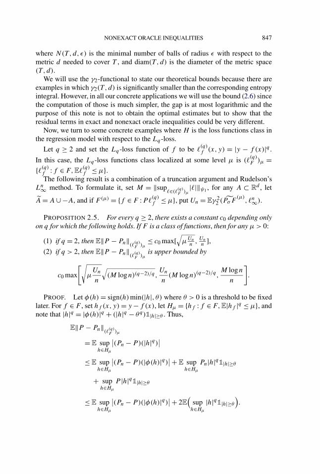
where N(T ,d, ε) is the minimal number of balls of radius ε with respect to themetric d needed to cover T , and diam(T , d) is the diameter of the metric space(T , d).
We will use the γ2-functional to state our theoretical bounds because there areexamples in which γ2(T , d) is significantly smaller than the corresponding entropyintegral. However, in all our concrete applications we will use the bound (2.6) sincethe computation of those is much simpler, the gap is at most logarithmic and thepurpose of this note is not to obtain the optimal estimates but to show that theresidual terms in exact and nonexact oracle inequalities could be very different.
Now, we turn to some concrete examples where H is the loss functions class inthe regression model with respect to the Lq -loss.
Let q ≥ 2 and set the Lq -loss function of f to be !(q)f (x, y) = |y − f (x)|q .
In this case, the Lq -loss functions class localized at some level µ is (!(q)F )µ =
{!(q)f :f ∈ F,E!(q)
f ≤ µ}.The following result is a combination of a truncation argument and Rudelson’s
Ln∞ method. To formulate it, set M = ‖sup
!∈(!(q)F )µ
|!|‖ψ1 , for any A ⊂ Rd , let
A = A∪−A, and if F (µ) = {f ∈ F :P !(q)f ≤ µ}, put Un = Eγ 2
2 (PσF(µ)
,!n∞).
PROPOSITION 2.5. For every q ≥ 2, there exists a constant c0 depending onlyon q for which the following holds. If F is a class of functions, then for any µ > 0:
(1) if q = 2, then E‖P − Pn‖(!(q)F )µ
≤ c0 max[√
µUnn , Un
n ],(2) if q > 2, then E‖P − Pn‖(!(q)
F )µis upper bounded by
c0 max
[√
µUn
n
√(M logn)(q−2)/q,
Un
n(M logn)(q−2)/q,
M logn
n
]
.
PROOF. Let φ(h) = sign(h)min(|h|, θ) where θ > 0 is a threshold to be fixedlater. For f ∈ F , set hf (x, y) = y−f (x), let Hµ = {hf :f ∈ F,E|hf |q ≤ µ}, andnote that |h|q = |φ(h)|q + (|h|q − θq)1|h|≥θ . Thus,
E‖P − Pn‖(!(q)F )µ
= E suph∈Hµ
∣∣(Pn − P)(|h|q)∣∣
≤ E suph∈Hµ
∣∣(Pn − P)(|φ(h)|q)∣∣ + E sup
h∈Hµ
Pn|h|q1|h|≥θ
+ suph∈Hµ
P |h|q1|h|≥θ
≤ E suph∈Hµ
∣∣(Pn − P)(|φ(h)|q)∣∣ + 2E
(sup
h∈Hµ
|h|q1|h|≥θ).

848 G. LECUÉ AND S. MENDELSON
To upper bound the truncated part of the process, consider the empirical di-ameter Dn = suph∈Hµ
(Pn|φ(h)|2q−2)1/(2q−2). By the Ziné–Ginn symmetrizationtheorem [42] and the upper bound on a Rademacher process by a Gaussian one,
E suph∈Hµ
∣∣(Pn − P)(|φ(h)|q)∣∣≤ c0√
nEEg sup
h∈Hµ
∣∣∣∣∣1√n
n∑
i=1
gi |φ(h)(Xi, Yi)|q∣∣∣∣∣,
where g1, . . . , gn are n independent standard random variables and Eg denotesthe expectation with respect to those variables. For a fixed sample (Xi, Yi)
ni=1, let
(Z(h))h∈Hµ be the Gaussian process defined by Z(h) = n−1/2 ∑ni=1 gi |φ(h)(Xi ,
Yi)|q . If f,g ∈ F , then
Eg(Z(hf )−Z(hg)
)2
= 1n
n∑
i=1
(|φ(hf )(Xi, Yi)|q − |φ(hg)(Xi, Yi)|q)2
≤ 1n
n∑
i=1
q2|f (Xi)− g(Xi)|2 max(|φ(hf )(Xi, Yi)|, |φ(hg)(Xi, Yi)|)2q−2
≤ 2q2 max1≤i≤n
(f (Xi)− g(Xi)
)2D2q−2
n ,
where we have used that ||φ(u)|q − |φ(v)|q | ≤ q|u − v|max(|φ(u)|, |φ(v)|)q−1
for every u, v ∈R. By a standard chaining argument it follows that
Eg supf∈F (µ)
∣∣∣∣∣1√n
n∑
i=1
gi |φ(hf )(Xi, Yi)|q∣∣∣∣∣≤ c1qγ2
(PσF (µ),!n
∞)Dq−1
n(2.7)
and thus, E suph∈Hµ|(Pn − P)(|φ(h)|q)|≤ c2q
√Eγ 2
2 (PσF (µ),!n∞)
n
√ED
2q−2n .
A bound on the diameter follows from (2.7) and the contraction principle,
ED2q−2n ≤ E sup
h∈Hµ
∣∣(Pn − P)(|φ(h)|2q−2)∣∣ + sup
h∈Hµ
P |φ(h)|2q−2
≤ c2qθq−2
√n
Eg suph∈Hµ
∣∣∣∣∣1√n
n∑
i=1
gi |φ(h)(Xi, Yi)|q∣∣∣∣∣ + θq−2µ
≤ c2qθq−2
√UnED
2q−2n
n+ θq−2µ,
implying that ED2q−2n ≤ c3 max(q2θ2q−4Un/n, θq−2µ) and so
E suph∈Hµ
∣∣(Pn − P)(|φ(h)|q)∣∣≤ c4q max
(qUnθ
q−2
n,
√Unθq−2µ
n
)
.(2.8)
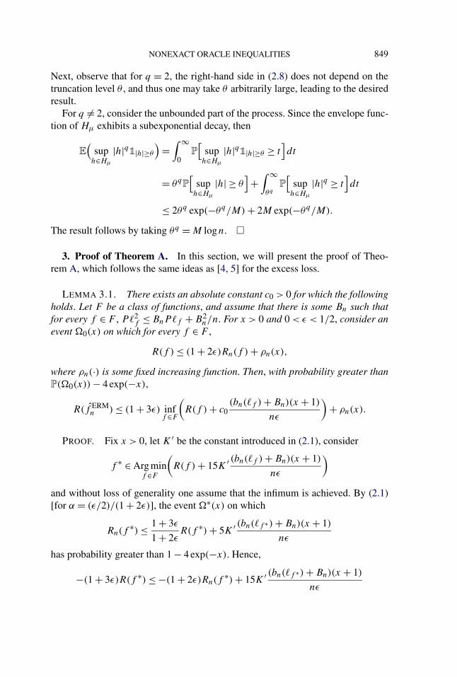
NONEXACT ORACLE INEQUALITIES 849
Next, observe that for q = 2, the right-hand side in (2.8) does not depend on thetruncation level θ , and thus one may take θ arbitrarily large, leading to the desiredresult.
For q (= 2, consider the unbounded part of the process. Since the envelope func-tion of Hµ exhibits a subexponential decay, then
E(
suph∈Hµ
|h|q1|h|≥θ)
=∫ ∞
0P
[sup
h∈Hµ
|h|q1|h|≥θ ≥ t]dt
= θqP[
suph∈Hµ
|h|≥ θ]+
∫ ∞
θqP
[sup
h∈Hµ
|h|q ≥ t]dt
≤ 2θq exp(−θq/M) + 2M exp(−θq/M).
The result follows by taking θq = M logn. "
3. Proof of Theorem A. In this section, we will present the proof of Theo-rem A, which follows the same ideas as [4, 5] for the excess loss.
LEMMA 3.1. There exists an absolute constant c0 > 0 for which the followingholds. Let F be a class of functions, and assume that there is some Bn such thatfor every f ∈ F , P !2
f ≤ BnP !f + B2n/n. For x > 0 and 0 < ε < 1/2, consider an
event /0(x) on which for every f ∈ F ,
R(f )≤ (1 + 2ε)Rn(f ) + ρn(x),
where ρn(·) is some fixed increasing function. Then, with probability greater thanP(/0(x))− 4 exp(−x),
R(f ERMn )≤ (1 + 3ε) inf
f∈F
(R(f ) + c0
(bn(!f ) + Bn)(x + 1)
nε
)+ ρn(x).
PROOF. Fix x > 0, let K ′ be the constant introduced in (2.1), consider
f ∗ ∈Arg minf∈F
(R(f ) + 15K ′ (bn(!f ) + Bn)(x + 1)
nε
)
and without loss of generality one assume that the infimum is achieved. By (2.1)[for α = (ε/2)/(1 + 2ε)], the event /∗(x) on which
Rn(f∗)≤ 1 + 3ε
1 + 2εR(f ∗) + 5K ′ (bn(!f ∗) + Bn)(x + 1)
nε
has probability greater than 1− 4 exp(−x). Hence,
−(1 + 3ε)R(f ∗)≤−(1 + 2ε)Rn(f∗) + 15K ′ (bn(!f ∗) + Bn)(x + 1)
nε

850 G. LECUÉ AND S. MENDELSON
and on /0(x)∩/∗(x), every f in F satisfies that
R(f )− (1 + 3ε)R(f ∗)≤ (1 + 2ε)(Rn(f )−Rn(f
∗)) + ρn(x)
+ 15K ′ (bn(!f ∗) + Bn)(x + 1)
nε.
Since Rn(fERMn )−Rn(f
∗)≤ 0, then
R(f ERMn )≤ (1 + 3ε)R(f ∗) + 15K ′ (bn(!f ∗) + Bn)(x + 1)
nε+ ρn(x),
and the claim now follows from the choice of f ∗. "
PROOF OF THEOREM A. Let x > 0, 0 < ε < 1/2, and put
ρn(x) = max(λ∗ε ,
((6K/ε)2Bn + (4K/ε)bn(!F ))(x + 1)
n
).
By Theorem 2.2, the event /0(x), on which every f ∈ F satisfies that
R(f )≤ (1 + 2ε)Rn(f ) + ρn(x),
has probability greater than 1 − 4 exp(−x). Now, the result follows from Lem-ma 3.1.
The remark following Theorem A, that if ! is nonnegative, then !F satisfiesa Bernstein-type condition with Bn ∼ diam(!F ,ψ1) log(en) follows from Lem-ma 2.3. "
4. Proof of Theorem B. Although the proof of Theorem B seems rather tech-nical, the idea behind it is rather simple. First, one needs to find a “trivial” boundon crit(f RERM
n ), giving preliminary information on where one must look for theRERM function (this is the role played by the function αn). Then, one combinespeeling and fixed point arguments to identify the exact location of the RERM.
Note that for F = ⋃r≥0 Fr , we have crit(f ) =∞ for all f ∈ F \ F . Therefore,
without loss of generality, we can replace the set F by F in both the definition ofthe RERM in (1.4) and in the nonexact regularized oracle inequality of Theorem B.
We begin with the following rough estimate on the criterion of the RERM. Inthe case where there is a trivial bound crit(f ) ≤ Cn, for all f ∈ F then it followsthat for any 0 < ε < 1/2 and x > 0, crit(f RERM
n ) ≤ Cn = αn(ε, x). Turning tothe second case stated in Assumption 1.1, recall that r → λ∗ε(r) tends to infinitywith r and there exists K1 > 0 such that for every (r, x) ∈ R+ ×R∗+, 2ρn(r, x)≤ρn(K1(r + 1), x). Hence, for every x > 0 and 0 < ε < 1/2, we set αn to satisfythat
αn(ε, x)≥max[K1
(crit(f0) + 2
),
(λ∗ε)−1(
(1 + 2ε)(3R(f0) + 2K ′(bn(!f0) + Bn(crit(f0))
)
× ((x + 1)/n
)))],

NONEXACT ORACLE INEQUALITIES 851
where f0 is any fixed function in F (e.g., when 0 ∈ F , one may take f0 = 0),and (λ∗ε)
−1 is the generalized inverse function of λ∗ε . In this case, we prove thefollowing high probability bound on crit(f RERM
n ).
LEMMA 4.1. Assume that r → λ∗ε(r) tends to infinity when r tends to infinityand that there exists K1 > 0 such that for every (r, x) ∈ R+ × R∗+, 2ρn(r, x) ≤ρn(K1(r + 1), x). Then, under the assumptions of Theorem B, for every x > 0 and0 < ε < 1/2, with probability greater than 1−4 exp(−x), crit(f RERM
n )≤ αn(ε, x).
PROOF. By the definition of f RERMn ,
Rn(fRERMn ) + 2
1 + 2ερn
(crit(f RERM
n ) + 1, x + logαn(ε, x))
≤Rn(f0) + 21 + 2ε
ρn(crit(f0) + 1, x + logαn(ε, x)
).
Since ! is nonnegative, then Rn(fRERMn )≥ 0, and thus
ρn(crit(f RERM
n ) + 1, x + logαn(ε, x))
≤ (1 + 2ε)Rn(f0)/2 + ρn(crit(f0) + 1, x + logαn(ε, x)
)
≤max((1 + 2ε)Rn(f0),2ρn
(crit(f0) + 1, x + logαn(ε, x)
)).
Since ρn(r, x) ≥ λ∗ε(r), for all r ≥ 0, one of the following two situations occurs:either
λ∗ε(crit(f RERMn ))≤ (1 + 2ε)Rn(f0)
or, noting that for every (r, x) ∈R+ ×R∗+, 2ρn(r, x)≤ ρn(K1(r + 1), x), then
ρn(crit(f RERM
n ) + 1, x + logαn(ε, x))
≤ 2ρn(crit(f0) + 1, x + logαn(ε, x)
)
≤ ρn(K1
(crit(f0) + 2
), x + logαn(ε, x)
),
and since ρn is monotone in r then crit(f RERMn )≤K1(crit(f0) + 2).
Hence, in both cases
crit(f RERMn )≤max
((λ∗ε)
−1((1 + 2ε)Rn(f0)
),K1
(crit(f0) + 2
)).(4.1)
On the other hand, according to (2.1), with probability greater than 1 −4 exp(−x), Rn(f0) ≤ 3R(f0) + 2K ′(bn(!f0) + Bn(crit(f0)))(x + 1)/n. The re-sult follows by plugging the last inequality in (4.1) and since λε is nondecreasing.
"
The next step is to find an “isomorphic” result for f RERMn . The idea is to divide
the set given by the trivial estimate on crit(f RERMn ) into level sets and analyze each
piece separately.

852 G. LECUÉ AND S. MENDELSON
LEMMA 4.2. Under the assumptions of Theorem B, for every x > 0, withprobability greater than 1− 8 exp(−x),
R(f RERMn )≤ (1 + 2ε)Rn(f
RERMn ) + ρn
(crit(f RERM
n ) + 1, x + logαn(ε, x)).
PROOF. Let /0(x) be the event
R(f RERMn )−Rn(f
RERMn )
2εRn(f RERMn ) + ρn(crit(f RERM
n ) + 1, x + logαn(ε, x))≥ 1,
and we will show that this event has the desired small probability.Clearly,
P[/0(x)]≤ P[/0(x)∩ {crit(f RERMn )≤ αn(ε, x)}] + P[crit(f RERM
n ) > αn(ε, x)],
and by Lemma 4.1, P[crit(f RERMn ) > αn(ε, x)]≤ 4 exp(−x) in the second case of
Assumption 1.1 or P[crit(f RERMn ) > αn(ε, x)] = 0 when there is a trivial bound
on the criterion. Therefore, in any case, we have P[crit(f RERMn ) > αn(ε, x)] ≤
4 exp(−x).Recall that Fi = {f ∈ F : crit(f ) ≤ i}, for all i ∈ N, and since ρn is monotone
in r , then
P[/0(x)∩ {crit(f RERMn )≤ αn(ε, x)}]
≤4αn(ε,x)5∑
i=0
P[/0(x)∩ {i ≤ crit(f RERMn )≤ i + 1}]
≤4αn(ε,x)5∑
i=0
P[∃f ∈ Fi+1 :
R(f )≥ (1 + 2ε)Rn(f ) + ρn(i + 1, x + logαn(ε, x)
)].
By Theorem 2.2, for every t > 0 and i ∈ N, with probability greater than 1−4 exp(−t), for every f ∈ Fi+1, P !f ≤ (1 + 2ε)Pn!f + ρn(i + 1, t). In particular,
P[∃f ∈ Fi+1 :R(f )≥ (1 + 2ε)Rn(f ) + ρn
(i + 1, x + logαn(ε, x)
)]
≤ 4 exp(−(
x + logαn(ε, x)))
.
Hence, the claim follows, since
P[/0(x)∩ {crit(f RERMn )≤ αn(ε, x)}]
≤4αn(ε,x)5∑
i=0
4 exp(−(
x + logαn(ε, x)))≤ 4 exp(−x).
"

NONEXACT ORACLE INEQUALITIES 853
PROOF OF THEOREM B. Let x > 0 and 0 < ε < 1. Without loss of generality,we assume that, for the constant K ′ defined in (2.1), there exists f ∗ ∈ F minimiz-ing the function
f ∈ F −→ (1 + 3ε)R(f ) + ρn(crit(f ) + 1, x + logαn(ε, x)
)
+ 6K ′ (bn(!f ) + Bn(crit(f ))(x + 1)
εn.
Let /∗(x) be the event on which
Rn(f∗)≤ 1 + 3ε
1 + 2εR(f ∗) + K ′ (bn(!f ∗) + Bn(crit(f ∗)))(x + 1)
n
(1 + 3εε
).
Since f ∗ ∈ Fcrit(f ∗), then P !2f ∗ ≤ Bn(crit(f ∗))P !f ∗ + B2
n(crit(f ∗))/n, and by(2.1) [applied with α = ε/(1 + 2ε)], P(/∗(x))≥ 1− 4 exp(−x).
Consider the event /0(x), on which
R(f RERMn )≤ (1 + 2ε)Rn(f
RERMn )
+ ρn(crit(f RERM
n ) + 1, x + logαn(ε, x))
and observe that by Lemma 4.2, P[/0(x)]≥ 1−8 exp(−x). Therefore, on /0(x)∩/∗(x), we have
R(f RERMn ) + ρn
(crit(f RERM
n ) + 1, x + logαn(ε, x))
− (1 + 3ε)R(f ∗)
≤ (1 + 2ε)(Rn(f
RERMn )−Rn(f
∗))
+ 2ρn(crit(f RERM
n ) + 1, x + logαn(ε, x))
+ 6K ′ (bn(!f ∗) + Bn(crit(f ∗)))(x + 1)
εn
≤ (1 + 2ε)(Rn(f
RERMn ) + 2
1 + 2ερn
(crit(f RERM
n ) + 1, x + logαn(ε, x))
−Rn(f∗)− 2
1 + 2ερn
(crit(f ∗) + 1, x + logαn(ε, x)
))
+ 2ρn(crit(f ∗) + 1, x + logαn(ε, x)
)
+ 6K ′ (bn(!f ∗) + Bn(crit(f ∗)))(x + 1)
εn
≤ 2ρn(crit(f ∗) + 1, x + logαn(ε, x)
)
+ 6K ′ (bn(!f ∗) + Bn(crit(f ∗)))(x + 1)
εn,
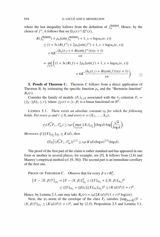
854 G. LECUÉ AND S. MENDELSON
where the last inequality follows from the definition of f RERMn . Hence, by the
choice of f ∗, it follows that on /1(x)∩/∗(x),
R(f RERMn ) + ρn
(crit(f RERM
n ) + 1, x + logαn(ε, x))
≤ (1 + 3ε)R(f ∗) + 2ρn(crit(f ∗) + 1, x + logαn(ε, x)
)
+ 6K ′ (bn(!f ∗) + B(crit(f ∗)))(x + 1)
εn
= inff∈F
((1 + 3ε)R(f ) + 2ρn
(crit(f ) + 1, x + logαn(ε, x)
)
+ 6K ′ (bn(!f ) + B(crit(f )))(x + 1)
εn
). "
5. Proofs of Theorem C. Theorem C follows from a direct application ofTheorem B, by estimating the specific function ρn and the “Bernstein function”Bn(r).
Consider the family of models (Fr)r≥0 associated with the !1-criterion Fr ={fβ :‖β‖1 ≤ r}, where fβ(x) = 〈x,β〉 is a linear functional on Rd .
LEMMA 5.1. There exists an absolute constant c0 for which the followingholds. For every µ and r ≥ 0, and every σ = (X1, . . . ,Xn),
γ2(PσF r,!n∞)≤ c0r
(max
1≤i≤n‖Xi‖!d∞
)(logd) log
( √n
logd
).
Moreover, if ‖‖X‖!d∞‖ψ2 ≤K(d), then
(Eγ 22 (PσF r,!
n∞))1/2 ≤ c0rK(d)(logn)3/2(logd).
The proof of the first part of the claim is rather standard and has appeared in oneform or another in several places; for example, see [5]. It follows from (2.6) andMaurey’s empirical method (cf. [9, 36]). The second part is an immediate corollaryof the first one.
PROOF OF THEOREM C. Observe that for every β ∈ rBd1 ,
∥∥|Y − 〈X,β〉|q∥∥ψ1
= ‖Y − 〈X,β〉‖qψq≤ (‖Y‖ψq + ‖〈X,β〉‖ψq )
q
≤ (‖Y‖ψq + ‖β‖1‖‖X‖∞‖ψq )q ≤ (K(d))q(1 + r)q.
Hence, by Lemma 2.3, one may take Bn(r) = c0(2K(d))q(1 + r)q log(en).Next, the ψ1-norm of the envelope of the class Fr satisfies ‖supβ∈rBd
1|Y −
〈X,β〉|q‖ψ1 ≤ (K(d))q(1 + r)q , and by (2.5), Proposition 2.5 and Lemma 5.1,

NONEXACT ORACLE INEQUALITIES 855
for every λ > 0,
E‖P − Pn‖V (!(q)Fr
)λ
≤∞∑
i=0
2−iE‖P − Pn‖(!(q)Fr
)2i+1λ
≤ c0
∞∑
i=0
2−i max
(√2i+1λ
√r2(1 + r)q−2h(n, d)
n,
r2(1 + r)q−2h(n, d)
n,K(d)q(1 + r)q(logn)
n
)
≤ c1 max
(√λ
√(1 + r)qh(n, d)
n,(1 + r)qh(n, d)
n
)
,
where h(n, d) = K(d)q(logn)(4q−2)/q(logd)2. Set λ∗ε(r) = c2(1 + r)qh(n, d)/(nε2) and observe that E‖P − Pn‖V (!
(q)Fr
)λ∗ε (r)≤ (ε/4)λ∗ε(r). Since
bn(!(q)Fr
) =∥∥∥ max
1≤i≤nsupf∈Fr
!(q)f (Xi, Yi)
∥∥∥ψ1≤ c3(log en)
∥∥∥ supf∈Fr
!(q)f (X,Y )
∥∥∥ψ1
,
then one can take φn(r) = c3K(d)q(logn)(1 + r)q . Thus
ρn(r, x) = c4h(n, d)(1 + rq)
nε2 (1 + x)
is a valid isomorphic function for this problem. It is also easy to check that forf0 ≡ 0, logαn(ε, x) ≤ c5 log(max(x, n)‖Y‖qψq
). The result now follows by com-bining these estimates with Theorem B. "
6. Remarks on the differences between exact and nonexact oracle inequal-ities. The goal of this section is to describe the difference between the analysisused in [4] to obtain exact oracle inequalities for the ERM, and the one used in thisnote to establish nonexact oracle inequalities for the ERM (Theorem A). Our aimis to indicate why one may get faster rates for nonexact inequalities than for exactones for the same problem.
One should stress that this is not, by any means, a proof that it is impossibleto get exact oracle inequalities with fast rates (there are in fact examples in whichthe ERM satisfies exact oracle inequalities with fast rates: the linear aggregationproblem, [12]). It is not even a proof that the localization method presented hereis sharp. A detailed study of the isomorphic method and oracle inequalities for ageneral sub-Gaussian case (i.e., a sub-exponential squared loss), in the sense thatthe class F has a bounded diameter in Lψ2 rather than an envelope function, willbe presented in [27].

856 G. LECUÉ AND S. MENDELSON
However, we believe that this explanation will help to shed some light on thedifferences between the two types of inequalities, and we refer the reader to [27]for a more detailed and accurate analysis.
Our starting point is the following exact oracle inequality for ERM, which is amild modification of a result from [4]. The only difference is that it uses Adam-czak’s ψ1 version of Talagrand’s concentration inequality for empirical processes,instead of Massart’s version.
THEOREM 6.1. There exists an absolute constant c0 > 0 for which thefollowing holds. Let F be a class of functions and assume that there existsB > 0 such that for every f ∈ F , P L2
f ≤ BP Lf . Let µ∗ > 0 be such thatE‖Pn − P‖V (LF )µ∗ ≤ µ∗/8, and consider an increasing function ρn which satis-fies that, for every x > 0, ρn(x)≥max(µ∗, c0(bn(LF ) + B)x/n). Then, for everyx > 0, with probability greater than 1− 8 exp(−x), the risk of the ERM satisfiesR(f ERM
n )≤ inff∈F R(f ) + ρn(x).
Roughly put, and as indicated by the theorem, localization arguments are basedon two main components:
(1) A Bernstein-type condition, the essence of which is that it allows one to“translate” localization with respect to the loss or the excess loss to a localizationwith respect to a natural metric. In particular this leads to the necessary control onthe !n
2 diameter of a random coordinate projection of the localized class.(2) The fixed point of the empirical process indexed by the localized star-
shaped hull of the loss functions class (for nonexact inequalities) or of the excessloss functions class (for exact ones).
Although the two components seem similar for the exact and nonexact cases,they are very different. Indeed, for a nonexact oracle inequality, the Bernsteintype condition is almost trivially satisfied and requires no special properties on themodel/output couple (F,Y )—as long as the functions involved have well behavedtails. As such, it is an individual property of every class member; see Lemma 2.3.
On the other hand, the Bernstein condition required for the exact oracle inequal-ity is deeply connected to the geometry of the problem; see, for example, [30].More accurately, when the target Y is far from the set of multiple minimizers of therisk, N(F, !,X) = {Y : |{f ∈ F :R(f ) = inff∈F R(f )}|≥ 2}, one can show that aBernstein condition holds for a large variety of loss function !. However, when thetarget Y gets closer to the set N(F, !,X), the Bernstein constant B degenerates,and leads to rates slower than 1/
√n even if F is a two functions class. Hence, the
geometry of the problem (the relative position of Y and F ) is very important whentrying to establish exact oracle inequalities, and the Bernstein condition is truly a“global” property of F .
In particular, this explains the gap that we observed in the example precedingthe formulation of Theorem A. In that case, the class is a finite set of functions and
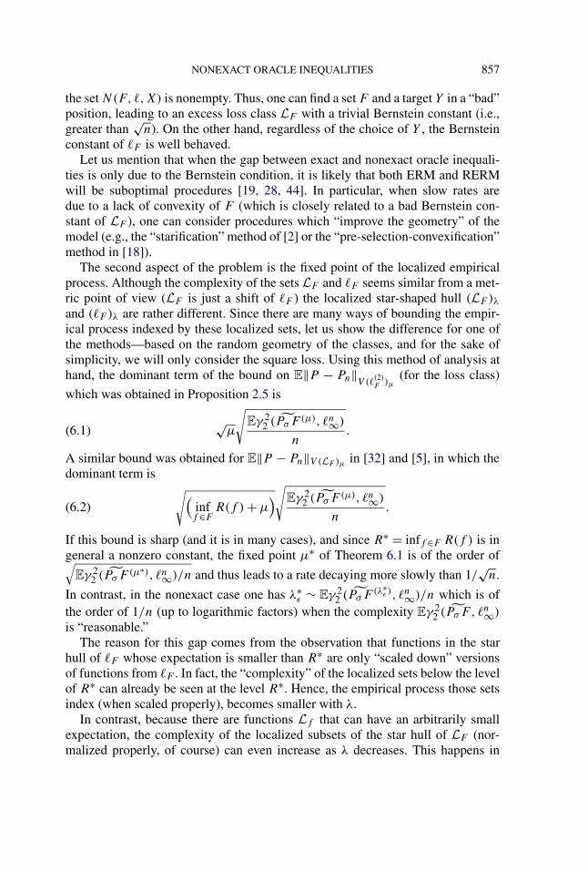
NONEXACT ORACLE INEQUALITIES 857
the set N(F, !,X) is nonempty. Thus, one can find a set F and a target Y in a “bad”position, leading to an excess loss class LF with a trivial Bernstein constant (i.e.,greater than
√n). On the other hand, regardless of the choice of Y , the Bernstein
constant of !F is well behaved.Let us mention that when the gap between exact and nonexact oracle inequali-
ties is only due to the Bernstein condition, it is likely that both ERM and RERMwill be suboptimal procedures [19, 28, 44]. In particular, when slow rates aredue to a lack of convexity of F (which is closely related to a bad Bernstein con-stant of LF ), one can consider procedures which “improve the geometry” of themodel (e.g., the “starification” method of [2] or the “pre-selection-convexification”method in [18]).
The second aspect of the problem is the fixed point of the localized empiricalprocess. Although the complexity of the sets LF and !F seems similar from a met-ric point of view (LF is just a shift of !F ) the localized star-shaped hull (LF )λand (!F )λ are rather different. Since there are many ways of bounding the empir-ical process indexed by these localized sets, let us show the difference for one ofthe methods—based on the random geometry of the classes, and for the sake ofsimplicity, we will only consider the square loss. Using this method of analysis athand, the dominant term of the bound on E‖P − Pn‖V (!
(2)F )µ
(for the loss class)which was obtained in Proposition 2.5 is
õ
√Eγ 2
2 (PσF (µ),!n∞)
n.(6.1)
A similar bound was obtained for E‖P − Pn‖V (LF )µ in [32] and [5], in which thedominant term is
√(inff∈F
R(f ) + µ)√
Eγ 22 (PσF (µ),!n∞)
n.(6.2)
If this bound is sharp (and it is in many cases), and since R∗ = inff∈F R(f ) is ingeneral a nonzero constant, the fixed point µ∗ of Theorem 6.1 is of the order of√
Eγ 22 (PσF (µ∗),!n∞)/n and thus leads to a rate decaying more slowly than 1/
√n.
In contrast, in the nonexact case one has λ∗ε ∼ Eγ 22 (PσF (λ∗ε ),!n
∞)/n which is ofthe order of 1/n (up to logarithmic factors) when the complexity Eγ 2
2 (PσF,!n∞)
is “reasonable.”The reason for this gap comes from the observation that functions in the star
hull of !F whose expectation is smaller than R∗ are only “scaled down” versionsof functions from !F . In fact, the “complexity” of the localized sets below the levelof R∗ can already be seen at the level R∗. Hence, the empirical process those setsindex (when scaled properly), becomes smaller with λ.
In contrast, because there are functions Lf that can have an arbitrarily smallexpectation, the complexity of the localized subsets of the star hull of LF (nor-malized properly, of course) can even increase as λ decreases. This happens in
858 G. LECUÉ AND S. MENDELSON
very simple situations; for example, even in regression relative to Bd1 , if R∗ (= 0,
the complexity of the localized sets remains almost stable and starts to decreaseonly at a very “low” level λ. This is the reason for the phase transition in the er-ror rate (∼max{√(logd)/n, d/n}) that one encounters in that problem. The firstterm is due to the fact that the complexity of the localized sets does not changeas λ decreases—up to some critical level, while the second captures what happenswhen the localized sets begin to “shrink.” A concrete example of this phenomenonis treated in the Supplementary material [20] in the Convex aggregation context.
SUPPLEMENTARY MATERIAL
Applications to matrix completion, convex aggregation and model selection(DOI: 10.1214/11-AOS965SUPP; .pdf). In the supplementary file, we apply ourmain results to the problem of matrix completion, convex aggregation and modelselection. The aim is to expose the fundamental differences between exact andnonexact oracle inequalities on classical problems.
REFERENCES
[1] ADAMCZAK, R. (2008). A tail inequality for suprema of unbounded empirical processes withapplications to Markov chains. Electron. J. Probab. 13 1000–1034. MR2424985
[2] AUDIBERT, J.-Y. (2007). No fast exponential deviation inequalities for the progressive mixturerule. Technical report, CERTIS.
[3] BARRON, A., BIRGÉ, L. and MASSART, P. (1999). Risk bounds for model selection via pe-nalization. Probab. Theory Related Fields 113 301–413. MR1679028
[4] BARTLETT, P. L. and MENDELSON, S. (2006). Empirical minimization. Probab. Theory Re-lated Fields 135 311–334. MR2240689
[5] BARTLETT, P. L., MENDELSON, S. and NEEMAN, J. (2012). !1-regularized linear regression:Persistence and oracle inequalities. Probab. Theory Related Fields. To appear.
[6] BICKEL, P. J., RITOV, Y. and TSYBAKOV, A. B. (2009). Simultaneous analysis of lasso andDantzig selector. Ann. Statist. 37 1705–1732. MR2533469
[7] BUNEA, F., TSYBAKOV, A. and WEGKAMP, M. (2007). Sparsity oracle inequalities for theLasso. Electron. J. Stat. 1 169–194. MR2312149
[8] CANDES, E. and TAO, T. (2007). The Dantzig selector: Statistical estimation when p is muchlarger than n. Ann. Statist. 35 2313–2351. MR2382644
[9] CARL, B. (1985). Inequalities of Bernstein–Jackson-type and the degree of compactness ofoperators in Banach spaces. Ann. Inst. Fourier (Grenoble) 35 79–118. MR0810669
[10] DONOHO, D. L. (2006). Compressed sensing. IEEE Trans. Inform. Theory 52 1289–1306.MR2241189
[11] GINÉ, E., LATAŁA, R. and ZINN, J. (2000). Exponential and moment inequalities for U -statistics. In High Dimensional Probability, II (Seattle, WA, 1999). Progress in Probability47 13–38. Birkhäuser, Boston, MA. MR1857312
[12] KOLTCHINSKII, V. (2006). Local Rademacher complexities and oracle inequalities in risk min-imization. Ann. Statist. 34 2593–2656. MR2329442
[13] KOLTCHINSKII, V. (2009). The Dantzig selector and sparsity oracle inequalities. Bernoulli 15799–828. MR2555200
[14] KOLTCHINSKII, V. (2009). Sparse recovery in convex hulls via entropy penalization. Ann.Statist. 37 1332–1359. MR2509076
NONEXACT ORACLE INEQUALITIES 859
[15] KOLTCHINSKII, V. (2009). Sparsity in penalized empirical risk minimization. Ann. Inst. HenriPoincaré Probab. Stat. 45 7–57. MR2500227
[16] KOLTCHINSKII, V. and PANCHENKO, D. (2000). Rademacher processes and bounding the riskof function learning. In High Dimensional Probability, II (Seattle, WA, 1999). Progress inProbability 47 443–457. Birkhäuser, Boston, MA. MR1857339
[17] LECUÉ, G. and MENDELSON, S. (2012). On the optimality of the aggregate with exponentialweights for low temperature. Bernoulli. To appear.
[18] LECUÉ, G. and MENDELSON, S. (2009). Aggregation via empirical risk minimization. Probab.Theory Related Fields 145 591–613. MR2529440
[19] LECUÉ, G. and MENDELSON, S. (2010). Sharper lower bounds on the performance of theempirical risk minimization algorithm. Bernoulli 16 605–613. MR2730641
[20] LECUÉ, G. and MENDELSON, S. (2012). Supplement to “General non-exact oracle inequalitiesfor classes with a subexponential envelope.” DOI:10.1214/11-AOS965SUPP.
[21] LEDOUX, M. and TALAGRAND, M. (1991). Probability in Banach Spaces: Isoperimetry andProcesses. Ergebnisse der Mathematik und Ihrer Grenzgebiete (3) [Results in Mathemat-ics and Related Areas (3)] 23. Springer, Berlin. MR1102015
[22] LOUNICI, K. (2008). Sup-norm convergence rate and sign concentration property of Lasso andDantzig estimators. Electron. J. Stat. 2 90–102. MR2386087
[23] MASSART, P. (2007). Concentration Inequalities and Model Selection. Lecture Notes in Math.1896. Springer, Berlin. MR2319879
[24] MASSART, P. and NÉDÉLEC, É. (2006). Risk bounds for statistical learning. Ann. Statist. 342326–2366. MR2291502
[25] MEINSHAUSEN, N. and BÜHLMANN, P. (2006). High-dimensional graphs and variable selec-tion with the lasso. Ann. Statist. 34 1436–1462. MR2278363
[26] MEINSHAUSEN, N. and YU, B. (2009). Lasso-type recovery of sparse representations for high-dimensional data. Ann. Statist. 37 246–270. MR2488351
[27] MENDELSON, S. Oracle inequalities and the isomorphic method. Technical report, Technion,Israel Inst. Technology.
[28] MENDELSON, S. (2008). Lower bounds for the empirical minimization algorithm. IEEE Trans.Inform. Theory 54 3797–3803. MR2451042
[29] MENDELSON, S. (2008). Lower bounds for the empirical minimization algorithm. IEEE Trans.Inform. Theory 54 3797–3803. MR2451042
[30] MENDELSON, S. (2008). Obtaining fast error rates in nonconvex situations. J. Complexity 24380–397. MR2426759
[31] MENDELSON, S. (2010). Empirical processes with a bounded ψ1 diameter. Geom. Funct. Anal.20 988–1027. MR2729283
[32] MENDELSON, S. and NEEMAN, J. (2010). Regularization in kernel learning. Ann. Statist. 38526–565. MR2590050
[33] MENDELSON, S., PAJOR, A. and TOMCZAK-JAEGERMANN, N. (2007). Reconstruction andsubgaussian operators in asymptotic geometric analysis. Geom. Funct. Anal. 17 1248–1282. MR2373017
[34] MENDELSON, S. and PAOURIS, G. (2011). On the generic chaining and the smallest sin-gular value of random matrices with heavy tails. Unpublished manuscript. Available atarXiv:1108.3886.
[35] NATARAJAN, B. K. (1995). Sparse approximate solutions to linear systems. SIAM J. Comput.24 227–234. MR1320206
[36] PISIER, G. (1981). Remarques sur un résultat non publié de B. Maurey. In Seminar on Func-tional Analysis, 1980–1981 Exp. No. V, 13. École Polytech., Palaiseau. MR0659306
[37] STEINWART, I. and CHRISTMANN, A. (2008). Support Vector Machines. Springer, New York.MR2450103

860 G. LECUÉ AND S. MENDELSON
[38] TALAGRAND, M. (1994). Sharper bounds for Gaussian and empirical processes. Ann. Probab.22 28–76. MR1258865
[39] TALAGRAND, M. (2005). The Generic Chaining: Upper and Lower Bounds of Stochastic Pro-cesses. Springer, Berlin. MR2133757
[40] TIBSHIRANI, R. (1996). Regression shrinkage and selection via the lasso. J. Roy. Statist. Soc.Ser. B 58 267–288. MR1379242
[41] VAN DE GEER, S. A. (2008). High-dimensional generalized linear models and the lasso. Ann.Statist. 36 614–645. MR2396809
[42] VAN DER VAART, A. W. and WELLNER, J. A. (1996). Weak Convergence and EmpiricalProcesses: With Applications to Statistics. Springer, New York. MR1385671
[43] VAPNIK, V. (1982). Estimation of Dependences Based on Empirical Data. Springer, New York.MR0672244
[44] WEE, S. L., BARTLETT, P. L. and WILLIAMSON, R. C. (1996). The importance of convexityin learning with squared loss. In Proceedings of the Ninth Annual Conference on Compu-tational Learning Theory 140–146. ACM Press, New York.
[45] ZHANG, T. (2009). Some sharp performance bounds for least squares regression with L1 reg-ularization. Ann. Statist. 37 2109–2144. MR2543687
[46] ZOU, H. (2006). The adaptive lasso and its oracle properties. J. Amer. Statist. Assoc. 101 1418–1429. MR2279469
CNRSLAMAUNIVERSITÉ PARIS-EST MARNE-LA-VALLÉE, 77454FRANCE
E-MAIL: [email protected]
DEPARTMENT OF MATHEMATICS
TECHNION, ISRAEL INSTITUTE OF TECHNOLOGY
HAIFA 32000ISRAEL
E-MAIL: [email protected]