General Multivariate Linear Modeling

of Surface Shapes Using SurfStat

Moo K. Chunga,b,e∗,Keith J. Worsleyd, Brendon, M. Nacewiczb,

Kim M. Daltonb, Richard J. Davidsonb,c

aDepartment of Biostatistics and Medical Informatics

bWaisman Laboratory for Brain Imaging and Behavior

cDepartment of Psychology and Psychiatry

University of Wisconsin, Madison, WI 53706, USA

dDepartment of Mathematics and Statistics

McGill University, Montreal, Canada

eDepartment of Brain and Cognitive Sciences

Seoul National University, Korea

May 4, 2010

Abstract

Although there are many imaging studies on traditional ROI-based amygdala volumetry,

there are very few studies on modeling amygdala shape variations. This paper present a uni-

fied computational and statistical framework for modeling amygdala shape variations in a

clinical population. The weighted spherical harmonic representation is used as to parameter-

ize, to smooth out, and to normalize amygdala surfaces. The representation is subsequently

used as an input for multivariate linear models accounting for nuisance covariates such as

∗Corresponding address: Moo K. Chung, Waisman Center #281, 1500 Highland

Ave. Madison, WI. 53705. telephone: 608-217-2452, email://mkhung@wisc.edu,

http://www.stat.wisc.edu/∼mchung

age and brain size difference using SurfStat package that completely avoids the complexity

of specifying design matrices. The methodology has been applied for quantifying abnormal

local amygdala shape variations in 22 high functioning autistic subjects.

Keywords: Amygdala, Spherical Harmonics, Fourier Analysis, Surface Flattening, Mul-

tivariate Linear Model, SurfStat

1. Introduction

Amygdala is an important brain substructure that has been implicated in abnormal func-

tional impairment in autism (Dalton et al., 2005; Nacewicz et al., 2006; Rojas et al., 2000).

Since structural abnormality might be the cause of the functional impairment, there have

been many studies on amygdala volumetry. However, previous amygdala volumetry results

have been inconsistent. Aylward et al. (1999) and Pierce et al. (2001) reported that amyg-

dala volume was significantly smaller in the autistic subjects while Howard et al. (2000) and

Sparks et al. (2002) reported larger volume. Haznedar et al. (2000) and Nacewicz et al.

(2006) found no volume difference. Schumann et al. (2004) reported that age dependent

amygdala volume difference in autistic children and indicated that the age dependency to be

the cause of discrepancy. All these previous studies traced the amygdalae manually and by

counting the number of voxels within the region of interest (ROI), the total volume of the

amygdala was estimated. The limitation of the traditional ROI-based volumetry is that it

can not determine if the volume difference is diffuse over the whole ROI or localized within

specific regions of the ROI (Chung et al., 2001). We present a novel computational and

statistical framework that enables localized amygdala shape characterization and able to

overcome the limitation of the ROI-based volumetry.

1.1 Previous Shape Models

Although there are extensive literature on local cortical shape analysis (Chung et al., 2005;

Fischl and Dale, 2000; Joshi et al., 1997; Taylor and Worsley, 2008; Thompson and Toga,

2

1996; Lerch and Evans, 2005; Luders et al., 2006; Miller et al., 2000), there are not many

literature on amygdala shape analysis other than Cates et al. (2008), Qiu et al. (2008) and

Khan et al. (1999) mainly due to the difficulty of segmenting amgydala. On the other hand,

there are extensive literature on shape modeling other subcortical structures using various

techniques.

The medial representation (Pizer et al., 1999) has been successfully applied to various

subcortical structures including the cross sectional images of the corpus callosum (Joshi

et al., 2002) and hippocampus/amygdala complex (Styner et al., 2003), and ventricle and

brain stem (Pizer et al., 1999). In the medial representation, the binary object is represented

using the finite number of atoms and links that connect the atoms together to form a skeletal

representation of the object. The medial representation is mainly used with the principal

component analysis type of approaches for shape classification and group comparison.

Unlike the medial representation, which is in a discrete representation, there is a continuous

parametric approach called the spherical harmonic representation (Gerig et al., 2001; Gu

et al., 2004; Kelemen et al., 1999; Shen et al., 2004). The spherical harmonic representation

has been mainly used as a data reduction technique for compressing global shape features

into a small number of coefficients. The main global geometric features are encoded in low

degree coefficients while the noise will be in high degree spherical harmonics (Gu et al., 2004).

The method has been used to model various subcortical structures such as ventricles (Gerig

et al., 2001), hippocampi (Shen et al., 2004) and cortical surfaces (Chung et al., 2007). The

spherical harmonics have global support. So the spherical harmonic coefficients contain only

the global shape features and it is not possible to directly obtain local shape information

from the coefficients only. However, it is still possible to obtain local shape information by

evaluating the representation at each fixed point, which gives the smoothed version of the

coordinates of surfaces. In this fashion, the spherical harmonic representation can be viewed

as mesh smoothing (Chung et al., 2007). Instead of using the global basis of spherical

harmonics, there have been attempts of using the local wavelet basis for parameterizing

3

cortical surfaces (Nain et al., 2007; Yu et al., 2007).

Other shape modeling approaches include distance transforms (Leventon et al., 2000),

deformation fields obtained by warping individual substructures to a template (Miller et al.,

1997) and the particle-based method (Cates et al., 2008). A distance transform is a function

that for each point in the image is equal to the distance from that point to the boundary of

the object (Golland et al., 2001). The distance map approach has been applied in classifying

a collection of hippocampi (Golland et al., 2001). The deformation fields based approach has

been somewhat popular and has been applied to modeling whole 3D brain volume (Ashburner

et al., 1998; Chung et al., 2001; Gaser et al., 1999), cortical surfaces (Chung et al., 2003;

Thompson et al., 2000), hippocampus (Joshi et al., 1997), and cingulate gyrus (Csernansky

et al., 2004). The particle-based method uses a nonparametric, dynamic particle system to

simultaneously sample object surfaces and optimize correspondence point positions (Cates

et al., 2008).

1.2 Available Computer Packages

Over the years, various neuroimage processing and analysis packages have been developed.

The SPM (www.fil.ion.ucl.ac.uk/spm) and AFNI (afni.nimh.nih.gov) software pack-

ages have been mainly designed for the whole brain volume based processing and massive

univariate linear model type of analyses. The traditional statistical inference is then used

to test hypotheses about the parameters of the model parameters. The subsequent multi-

ple comparisons problem is addressed using the random field theory or random simulations.

Although SPM and AFNI are probably two most widely used analysis tools, their analysis

pipelines are based on univariate general linear models and they do not have a routine for

a multivariate analysis. Therefore, they do not have the subsequent routine for correcting

multiple comparison corrections for the multivariate linear models as well.

There are also few surface based tools such as the surface mapper (SUMA) (Saad et al.,

2004) and FreeSurfer (surfer.nmr.mgh.harvard.edu). SUMA is a collection of mainly corti-

4

cal surface processing tools and does not have the support for multivariate linear models. The

spherical harmonic modeling tool SPHARM-PDM (www.nitrc.org/projects/spharm-pdm)

is also available (Styner et al., 2006). SPHARM-PDM supports for multivariate analysis of

covariance (MANCOVA), which is a subset of the more general multivariate linear modeling

framework.

For general multivariate linear modeling, one has to actually use statistical packages such

as Splus (www.insightful.com), R (www.r-project.org) and SAS (www.sas.com). These

statistical packages do not interface with imaging data easily so the additional processing step

is needed to read and write imaging data within the software. Further these tools do not have

the random field based multiple comparison correction procedures so the users are likely ex-

port analyzed statistics map to SPM or fMRISTAT (www.math.mcgill.ca/keith/fmristat)

increasing the burden of additional processing steps.

1.3 Our Contributions

In this paper, we use the weighted spherical harmonic representation for parameterization,

surface smoothing and surface registration in a unified Hilbert space framework. Chung

et al. (2007) presented the underlying mathematical theory and a new iterative algorithm

for estimating the coefficients of the representation for extremely large meshes such as cortical

surfaces. Here we apply the method to real autism surface data in a truly multivariate fashion

for the first time.

Our approach differs from the traditional spherical harmonic representation in many ways.

Although the truncation of the series expansion in the spherical harmonic representation can

be viewed as a form of smoothing, there is no direct equivalence to the full width at half

maximum (FWHM) usually associated with kernel smoothing. So it is difficult to relate the

unit of FWHM widely used in brain imaging to the degree of spherical harmonic representa-

tion. On the other hand, our new representation can easily relate to FWHM of smoothing

kernel so we have a clear sense of how much smoothing we are performing before hand.

5

The traditional representation suffers from the Gibbs phenomenon (ringing artifacts)

(Gelb, 1997) that usually happens in representing rapidly changing or discontinuous data

with smooth periodic basis. Our new representation can substantially reduce the amount of

Gibbs phenomenon by weighting the coefficients of the spherical harmonic expansion. The

weighting has the effect of actually performing heat kernel smoothing, and thus reducing the

ringing artifacts. We quantify the improved performance of our new representation in the

both real and simulated data using for the first time.

Since the proposed new representation requires a smooth map from amygdala surfaces to

a sphere, we have developed a new and very fast surface flattening technique based on the

propagation of heat diffusion. By tracing the integral curve of heat gradient from a heat

source (amygdala) to a heat sink (sphere), we can obtain the flattening map. Since solving

an isotropic heat equation in a 3D image volume is fairly straightforward, our proposed

method offers a much simpler numerical implementation than available surface flattening

techniques such as conformal mappings (Angenent et al., 1999; Gu et al., 2004; Hurdal and

Stephenson, 2004) quasi-isometric mappings (Timsari and Leahy, 2000) and area preserving

mappings (Brechbuhler et al., 1995). The established spherical mapping is used to parame-

terize an amygdala surface using two angles associated with the unit sphere. The angles serve

as coordinates for representing amygdala surfaces using the weighted linear combination of

spherical harmonics. The tools containing the weighted spherical harmonic representation

and the surface flattening algorithm can be found in

www.stat.wisc.edu/∼mchung/research/amygdala. It should be pointed out that our rep-

resentation and parameterization techniques are general enough to be applied to various

brain structures such as hippocampus and caudate that are topologically equivalent to a

sphere.

Based on the weighted spherical harmonic representation of amygdalae, various multivari-

ate tests were performed to detect the group difference between autistic and control subjects.

Most of multivariate shape models on coordinates and deformation vector fields have mainly

6

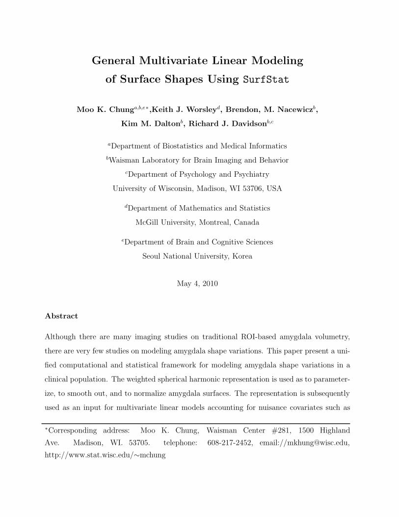
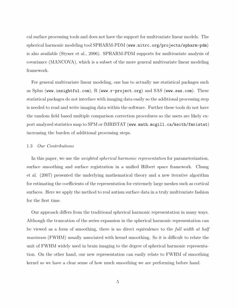
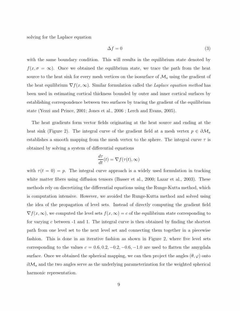
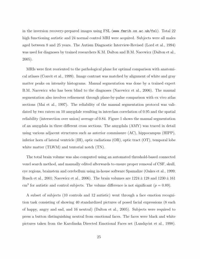
Figure 1. Amygdala manual segmentation at (a) axial (b) coronal and (c) midsagittal

sections. The amygdala (AMY) was segmented using adjacent structures such as anterior

commissure (AC), hippocampus (HIPP), inferior horn of lateral ventricle (IH), optic radi-

ations (OR), optic tract (OT), temporal lobe white matter (TLWM) and tentorial notch

(TN).

used the Hotelling’s T-sqaure as a test statistic (Cao and Worsley, 1999; Chung et al., 2001;

Collins et al., 1998; Gaser et al., 1999; Joshi et al., 1997; Thompson et al., 1997). The

Hotelling’s T-sqaure statistic tests for the equality of vector means without accounting the

additional covariates such as gender, brain size and age. Since the size of amygdala is de-

pendent on brain size and possibly on age as well, there is a definite need for a model that

is able to include these covariates explicitly. The proposed multivariate linear model does

exactly this by generalizing the Hotelling’s T-square framework to incorporate additional

covariates.

In order to simplify the computational burden of setting up the proposed multivariate lin-

ear models, we have developed the SurfStat package (www.math.mcgill.ca/keith/surfstat).

that offers a unified statistical analysis platform for various 2D surface mesh and 3D image

volume data. The novelty of SurfStat is that there is no need to specify design matrices

that tend to baffle researchers not familiar with contrasts and design matrices. SurfStat

supersedes fMRISTAT, and contains all the statistical and multiple comparison correction

routines.

7

2. Methods

2.1 Surface Parameterization

Once the binary segmentation Ma of an object is obtained either manually or automat-

ically, the marching cubes algorithm (Lorensen and Cline, 1987) was applied to obtain a

triangle surface mesh ∂Ma. The weighted spherical harmonic representation requires a

smooth mapping from the surface mesh to a unit sphere S2 to establish a coordinate system.

We have developed a new surface flattening algorithm based on heat diffusion.

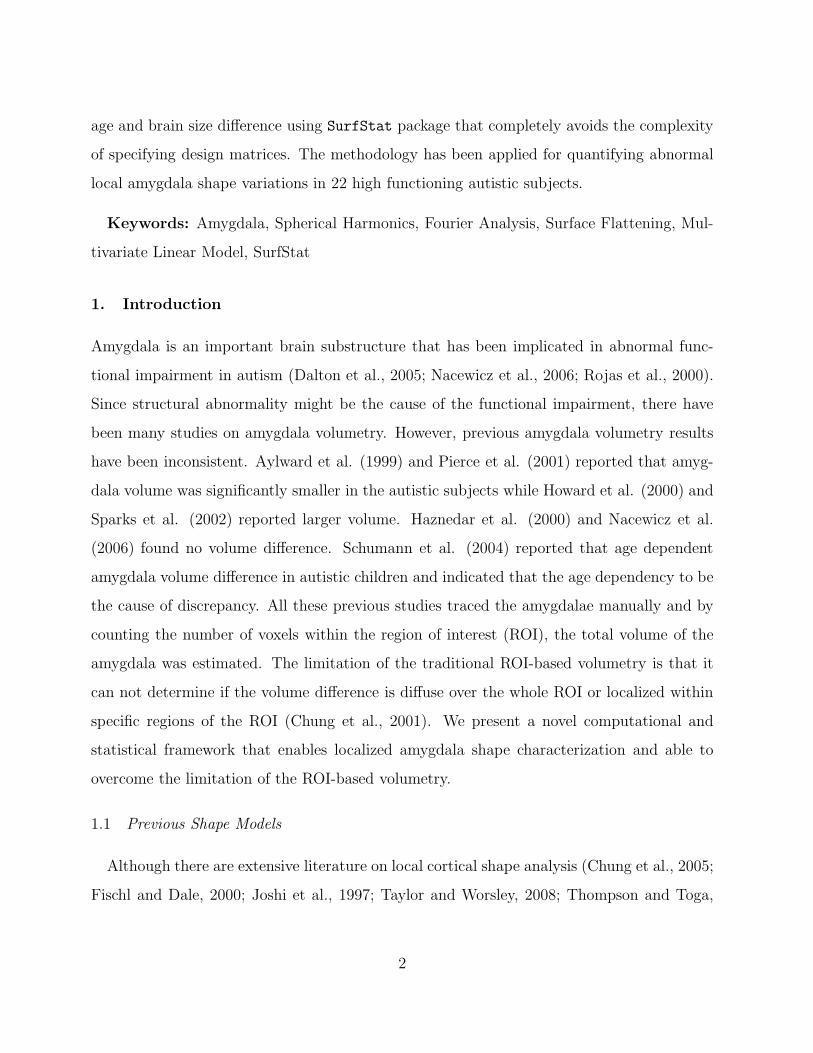
We start with putting a larger sphere Ms that encloses the binary object Ma. Figure 2

shows an illustration with the binary segmentation of amygdala. The center of the sphere

Ms is taken as the average of the mesh coordinates of ∂Ma, which forms the surface mass

center. The radius of the sphere Ms is taken in such a way that the shortest distance between

the sphere to the binary object Ma is fixed( 5mm for amygdale). The final flattening map

is definitely affected by the perturbation of the position of the sphere but since we are fixing

it to be the mass center of surface for all amygdale, we do not need to worry about the

perturbation effect.

The binary object Ma is assigned the value 1 while the enclosing sphere is assigned the

value -1, i.e.

f(Ma, σ) = 1 and f(Ms, σ) = −1 (1)

for all σ ∈ [0,∞). The parameter σ is the diffusion time. Ma and Ms serve as a heat source

and a heat sink respectively. Then we solve isotropic diffusion

∂f

∂σ= ∆f (2)

with the given boundary condition (1). ∆ is the 3D Laplacian. When σ → ∞, the solution

reaches the heat equilibrium state where the additional diffusion does not make any change

in heat distribution. The heat equilibrium state is also obtained by letting ∂f∂σ

= 0 and

8

solving for the Laplace equation

∆f = 0 (3)

with the same boundary condition. This will results in the equilibrium state denoted by

f(x, σ = ∞). Once we obtained the equilibrium state, we trace the path from the heat

source to the heat sink for every mesh vertices on the isosurface of Ma using the gradient of

the heat equilibrium ∇f(x,∞). Similar formulation called the Laplace equation method has

been used in estimating cortical thickness bounded by outer and inner cortical surfaces by

establishing correspondence between two surfaces by tracing the gradient of the equilibrium

state (Yezzi and Prince, 2001; Jones et al., 2006 ; Lerch and Evans, 2005).

The heat gradients form vector fields originating at the heat source and ending at the

heat sink (Figure 2). The integral curve of the gradient field at a mesh vertex p ∈ ∂Ma

establishes a smooth mapping from the mesh vertex to the sphere. The integral curve τ is

obtained by solving a system of differential equations

dτ

dt(t) = ∇f(τ(t),∞)

with τ(t = 0) = p. The integral curve approach is a widely used formulation in tracking

white matter fibers using diffusion tensors (Basser et al., 2000; Lazar et al., 2003). These

methods rely on discretizing the differential equations using the Runge-Kutta method, which

is computation intensive. However, we avoided the Runge-Kutta method and solved using

the idea of the propagation of level sets. Instead of directly computing the gradient field

∇f(x,∞), we computed the level sets f(x,∞) = c of the equilibrium state corresponding to

for varying c between -1 and 1. The integral curve is then obtained by finding the shortest

path from one level set to the next level set and connecting them together in a piecewise

fashion. This is done in an iterative fashion as shown in Figure 2, where five level sets

corresponding to the values c = 0.6, 0.2,−0.2,−0.6,−1.0 are used to flatten the amygdala

surface. Once we obtained the spherical mapping, we can then project the angles (θ, ϕ) onto

∂Ma and the two angles serve as the underlying parameterization for the weighted spherical

harmonic representation.

9

For the proposed flattening method to work, the binary object has to be close to either

star-shape or convex. For shapes with a more complex structure, the gradient lines that

correspond to neighboring nodes on the surface will fall within one voxel in the volume,

creating numerical singularities in mapping to the sphere. Other more complex mapping

methods such as conformal mapping (Angenent et al., 1999; Gu et al., 2004; Hurdal and

Stephenson, 2004) can avoid this problem but more numerically demanding. On the other

hands, our approach is simpler and more computationally efficient because it works for a

limited class of shapes.

2.2 Weighted Spherical Harmonic Representation

The parameterized amygdala surfaces, in terms of spherical angles θ, ϕ, are further ex-

pressed using the weighted spherical harmonic representation (Chung et al., 2007), which

expresses surface coordinate functions as a weighted linear combination of spherical harmon-

ics. The automatic degree selection procedure was also introduced in the previous work but

for the completeness of our paper, the method is briefly explained in section 2.3.

The mesh coordinates for the object surface ∂Ma are parameterized by the spherical

angles Ω = (θ, ϕ) ∈ [0, π] ⊗ [0, 2π) as

p(θ, ϕ) = (p1(θ, ϕ), p2(θ, ϕ), p2(θ, ϕ)).

The weighted spherical harmonic representation is given by

p(θ, ϕ) =

k∑

l=0

l∑

m=−l

e−l(l+1)σflmYlm(θ, ϕ),

where

flm =

∫ π

θ=0

∫ 2π

ϕ=0

p(θ, ϕ)Ylm(θ, ϕ) sin θdθdϕ

are the spherical harmonic coefficient vectors and Ylm are spherical harmonics of degree l

10

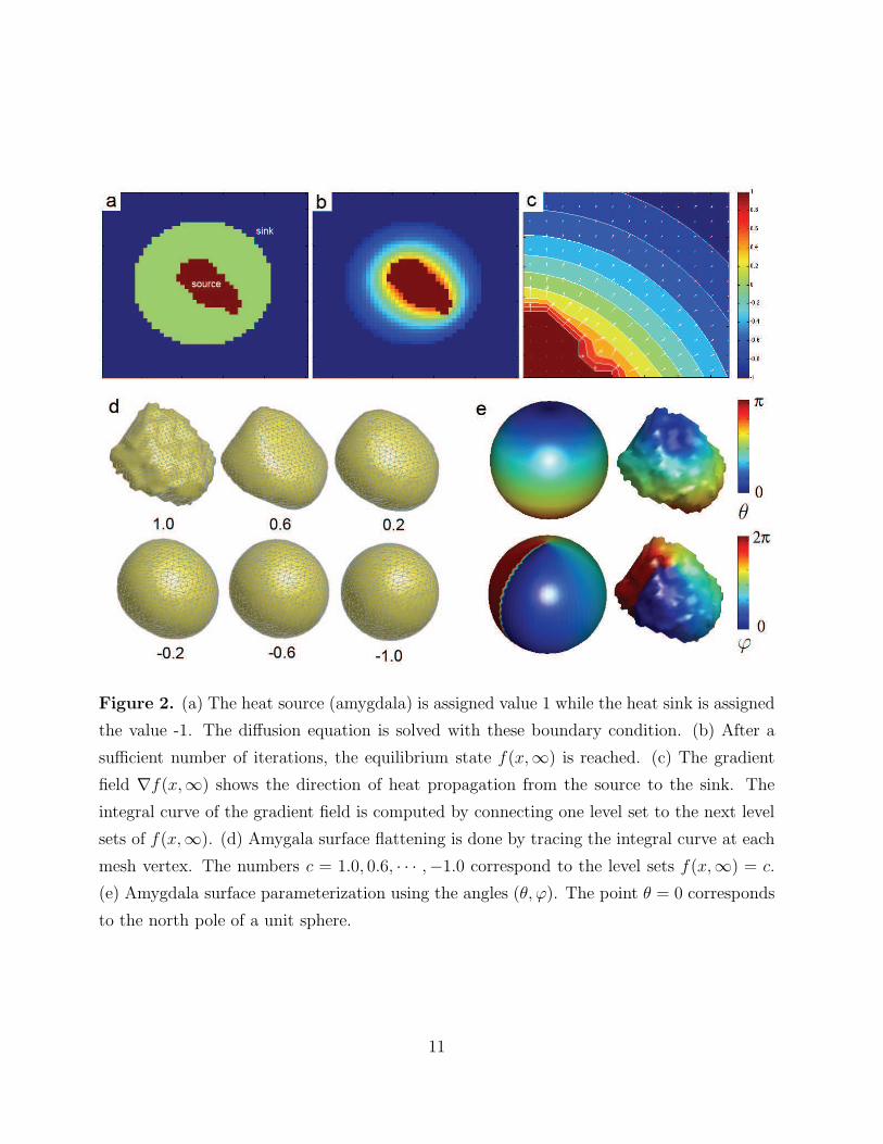
Figure 2. (a) The heat source (amygdala) is assigned value 1 while the heat sink is assigned

the value -1. The diffusion equation is solved with these boundary condition. (b) After a

sufficient number of iterations, the equilibrium state f(x,∞) is reached. (c) The gradient

field ∇f(x,∞) shows the direction of heat propagation from the source to the sink. The

integral curve of the gradient field is computed by connecting one level set to the next level

sets of f(x,∞). (d) Amygala surface flattening is done by tracing the integral curve at each

mesh vertex. The numbers c = 1.0, 0.6, · · · ,−1.0 correspond to the level sets f(x,∞) = c.

(e) Amygdala surface parameterization using the angles (θ, ϕ). The point θ = 0 corresponds

to the north pole of a unit sphere.

11

and order m defined as

Ylm =

clmP|m|l (cos θ) sin(|m|ϕ), −l ≤ m ≤ −1,

clm√2P

|m|l (cos θ), m = 0,

clmP|m|l (cos θ) cos(|m|ϕ), 1 ≤ m ≤ l,

where clm =√

2l+12π

(l−|m|)!(l+|m|)! and Pm

l is the associated Legendre polynomial of order m (Deflec-

tion, ). The associated Legendre polynomial is given by

Pml (x) =

(1 − x2)m/2

2ll!

dl+m

dxl+m(x2 − 1)l, x ∈ [−1, 1].

The first few terms of the spherical harmonics are

Y00 =1√4π, Y1,−1 =

√3

4πsin θ sinϕ,

Y1,0 =

√3

4πcos θ, Y1,1 =

√3

4πsin θ cosϕ.

The coefficients flm are estimated in a least squares fashion (Chung et al., 2007; Gerig et al.,

2001; Shen et al., 2004).

Many previous imaging and shape modeling literature have used the complex-valued spher-

ical harmonics (Bulow, 2004; Gerig et al., 2001; Gu et al., 2004; Shen et al., 2004), but we

have only used real-valued spherical harmonics (Deflection, ; Homeier and Steinborn, 1996)

throughout the paper for the convenience in setting up a real-valued stochastic model. The

relationship between the real- and complex-valued spherical harmonics is given in Blanco

et al. (1997), and Homeier and Steinborn (1996). The complex-valued spherical harmonics

can be transformed into real-valued spherical harmonics using an unitary transform.

In the subsequent multivariate linear modeling, some sort of surface smoothing is neces-

sary before the random field theory based multiple comparison correction is performed. One

important property of the weighted spherical harmonic representation is that the represen-

tation can be considered as kernel smoothing. On a unit sphere, the heat kernel is defined

as

Kσ(Ω,Ω′) =

∞∑

l=0

l∑

m=−l

e−l(l+1)σYlm(Ω)Ylm(Ω′). (4)

12

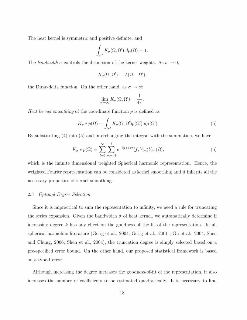
The heat kernel is symmetric and positive definite, and∫

S2

Kσ(Ω,Ω′) dµ(Ω) = 1.

The bandwidth σ controls the dispersion of the kernel weights. As σ → 0,

Kσ(Ω,Ω′) → δ(Ω − Ω′),

the Dirac-delta function. On the other hand, as σ → ∞,

limσ→∞

Kσ(Ω,Ω′) =1

4π.

Heat kernel smoothing of the coordinate function p is defined as

Kσ ∗ p(Ω) =

∫

S2

Kσ(Ω,Ω′)p(Ω′) dµ(Ω′). (5)

By substituting (4) into (5) and interchanging the integral with the summation, we have

Kσ ∗ p(Ω) =∞∑

l=0

l∑

m=−l

e−l(l+1)σ〈f, Ylm〉Ylm(Ω), (6)

which is the infinite dimensional weighted Spherical harmonic representation. Hence, the

weighted Fourier representation can be considered as kernel smoothing and it inherits all the

necessary properties of kernel smoothing.

2.3 Optimal Degree Selection

Since it is impractical to sum the representation to infinity, we need a rule for truncating

the series expansion. Given the bandwidth σ of heat kernel, we automatically determine if

increasing degree k has any effect on the goodness of the fit of the representation. In all

spherical harmolnic literature (Gerig et al., 2004; Gerig et al., 2001 ; Gu et al., 2004; Shen

and Chung, 2006; Shen et al., 2004), the truncation degree is simply selected based on a

pre-specified error bound. On the other hand, our proposed statistical framework is based

on a type-I error.

Although increasing the degree increases the goodness-of-fit of the representation, it also

increases the number of coefficients to be estimated quadratically. It is necessary to find

13

the optimal degree where the goodness-of-fit and the number of parameters balance out.

Consider the k-th degree error model:

p(Ω) =k−1∑

l=0

l∑

m=−l

e−l(l+1)σflmYlm(Ω) +k∑

m=−k

e−k(k+1)σfkmYkm(Ω) + ǫ(Ω), (7)

where ǫ is a zero mean Gaussian random field. We test if adding the k-th degree terms to

the k − 1-th degree model is statistically significant by formally testing

H0 : fk,−k = fk,−k+1 = · · · = fk,k−1 = fk,k = 0.

This can be easily done using the F statistic 2k + 1 and n − (k + 1)2 degrees of freedom.

At each degree, we compute the corresponding p-value and stop increasing the degree if it

is smaller than pre-specified significance α = 0.01. For bandwidths σ = 0.01, 0.001, 0.0001,

the approximate optimal degrees are 18, 42 and 78 respectively. In our study, we have used

k = 42 degree representation corresponding to bandwidth σ = 0.001. The bandwidth 0.01

smoothes out too much local details while the bandwidth 0.0001 introduces too much voxel

discretization error into the representation.

2.4 Reduction of Gibbs Phenomenon

The weighted spherical harmonic representation fixes the Gibbs phenomenon (ringing

effects) associated with the traditional Fourier descriptors and spherical harmonic repre-

sentation by weighting the series expansion with exponential weights (Chung et al., 2007).

The exponential weights make the representation converge faster and reduces the amount of

ringing artifacts. The Gibbs phenomenon often arises in Fourier series expansion of discrete

data.

To numerically quantify the amount of overshoot, we define the overshoot as the maximum

of L2 norm of the residual difference between the original and the reconstructed surface as

sup(θ,ϕ)∈S2

∣∣∣∣∣∣p(θ, ϕ) −

k∑

l=0

l∑

m=−l

e−l(l+1)σflmYlm(θ, ϕ)∣∣∣∣∣∣.

14

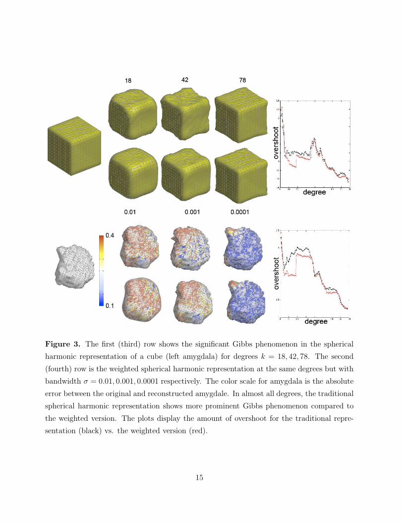
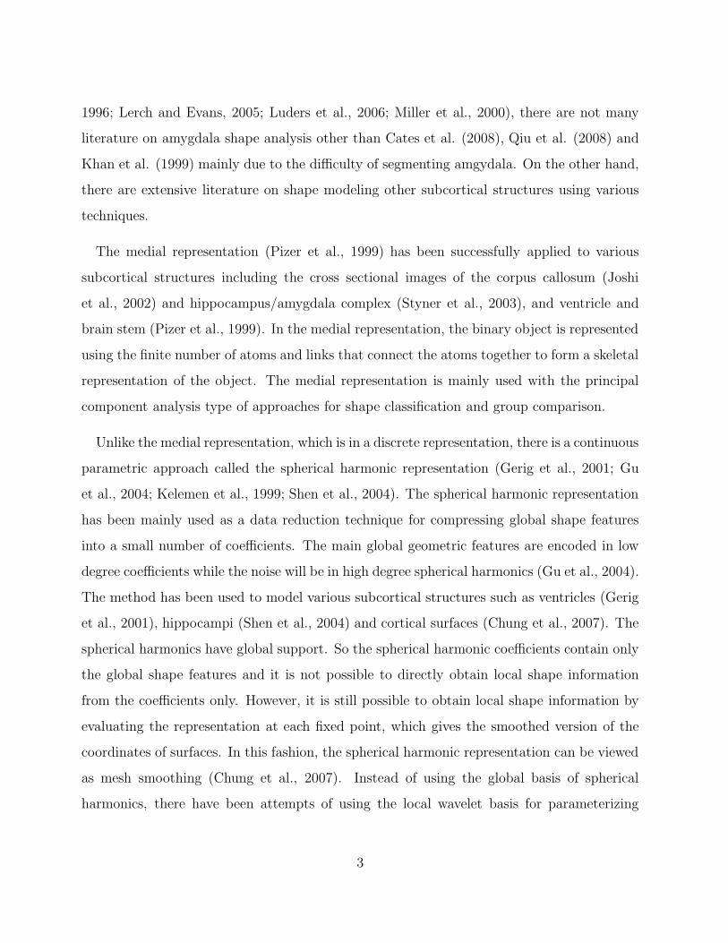
Figure 3. The first (third) row shows the significant Gibbs phenomenon in the spherical

harmonic representation of a cube (left amygdala) for degrees k = 18, 42, 78. The second

(fourth) row is the weighted spherical harmonic representation at the same degrees but with

bandwidth σ = 0.01, 0.001, 0.0001 respectively. The color scale for amygdala is the absolute

error between the original and reconstructed amygdale. In almost all degrees, the traditional

spherical harmonic representation shows more prominent Gibbs phenomenon compared to

the weighted version. The plots display the amount of overshoot for the traditional repre-

sentation (black) vs. the weighted version (red).

15

If surface coordinates are abruptly changing or their derivatives are discontinuous, the Gibbs

phenomenon will severely distort the surface shape and the overshoot will never converge to

zero.

We have reconstructed a cube and a left amygdala with various degree presentation and

the bandwidth showing more ringing artifacts and overshoot in the traditional representation

compared to the proposed weighted version. The exponentially decaying weights make the

representation converge faster and reduce the Gibbs phenomenon significantly. Figure 3

shows the comparison of overshoots between the two representations. The plots display the

amount of overshoot for the traditional representation (black) and the weighted version (red).

The weighted spherical harmonic representation shows less amount of overshoot compared

to the traditional technique.

2.5 Surface Normalization

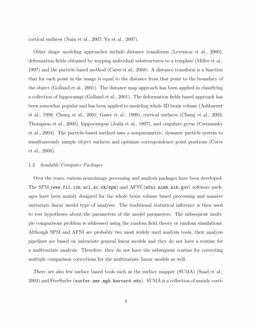
MRIs were first reoriented manually to the pathological plane for the manual binary seg-

mentation of amygdale (Convit et al., 1999). The images then further underwent a 6-

parameter rigid-body alignment with manual landmarking (Nacewicz et al., 2006). The

aligned left amygdale are displayed in Figure 4 showing an approximate initial alignment.

The the proposed weighted spherical harmonic representations were then obtained. The

additional alignment beyond the rigid-body alignment was done by matching the weighted

spherical harmonic representations. Note we are not trying to match the original noisy sur-

faces but rather their smooth analytic representations. The correspondence is established by

matching the coefficient of spherical harmonics at the same degree and order. This guaran-

tees the sum of squares errors to be minimum in the following sense. Consider two surface

coordinates p and q given by the representations

p(Ω) =k∑

l=0

l∑

m=−l

e−l(l+1)σflmYlm(Ω)

16

and

q(Ω) =

k∑

l=0

l∑

m=−l

e−l(l+1)σglmYlm(Ω),

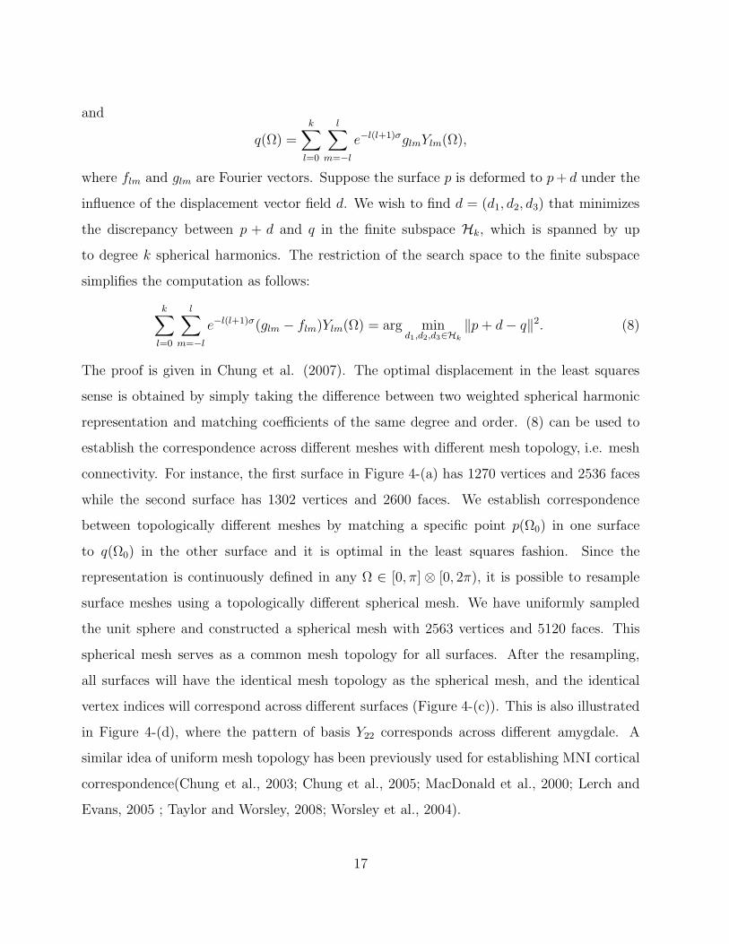
where flm and glm are Fourier vectors. Suppose the surface p is deformed to p+ d under the

influence of the displacement vector field d. We wish to find d = (d1, d2, d3) that minimizes

the discrepancy between p + d and q in the finite subspace Hk, which is spanned by up

to degree k spherical harmonics. The restriction of the search space to the finite subspace

simplifies the computation as follows:

k∑

l=0

l∑

m=−l

e−l(l+1)σ(glm − flm)Ylm(Ω) = arg mind1,d2,d3∈Hk

‖p+ d− q‖2. (8)

The proof is given in Chung et al. (2007). The optimal displacement in the least squares

sense is obtained by simply taking the difference between two weighted spherical harmonic

representation and matching coefficients of the same degree and order. (8) can be used to

establish the correspondence across different meshes with different mesh topology, i.e. mesh

connectivity. For instance, the first surface in Figure 4-(a) has 1270 vertices and 2536 faces

while the second surface has 1302 vertices and 2600 faces. We establish correspondence

between topologically different meshes by matching a specific point p(Ω0) in one surface

to q(Ω0) in the other surface and it is optimal in the least squares fashion. Since the

representation is continuously defined in any Ω ∈ [0, π] ⊗ [0, 2π), it is possible to resample

surface meshes using a topologically different spherical mesh. We have uniformly sampled

the unit sphere and constructed a spherical mesh with 2563 vertices and 5120 faces. This

spherical mesh serves as a common mesh topology for all surfaces. After the resampling,

all surfaces will have the identical mesh topology as the spherical mesh, and the identical

vertex indices will correspond across different surfaces (Figure 4-(c)). This is also illustrated

in Figure 4-(d), where the pattern of basis Y22 corresponds across different amygdale. A

similar idea of uniform mesh topology has been previously used for establishing MNI cortical

correspondence(Chung et al., 2003; Chung et al., 2005; MacDonald et al., 2000; Lerch and

Evans, 2005 ; Taylor and Worsley, 2008; Worsley et al., 2004).

17

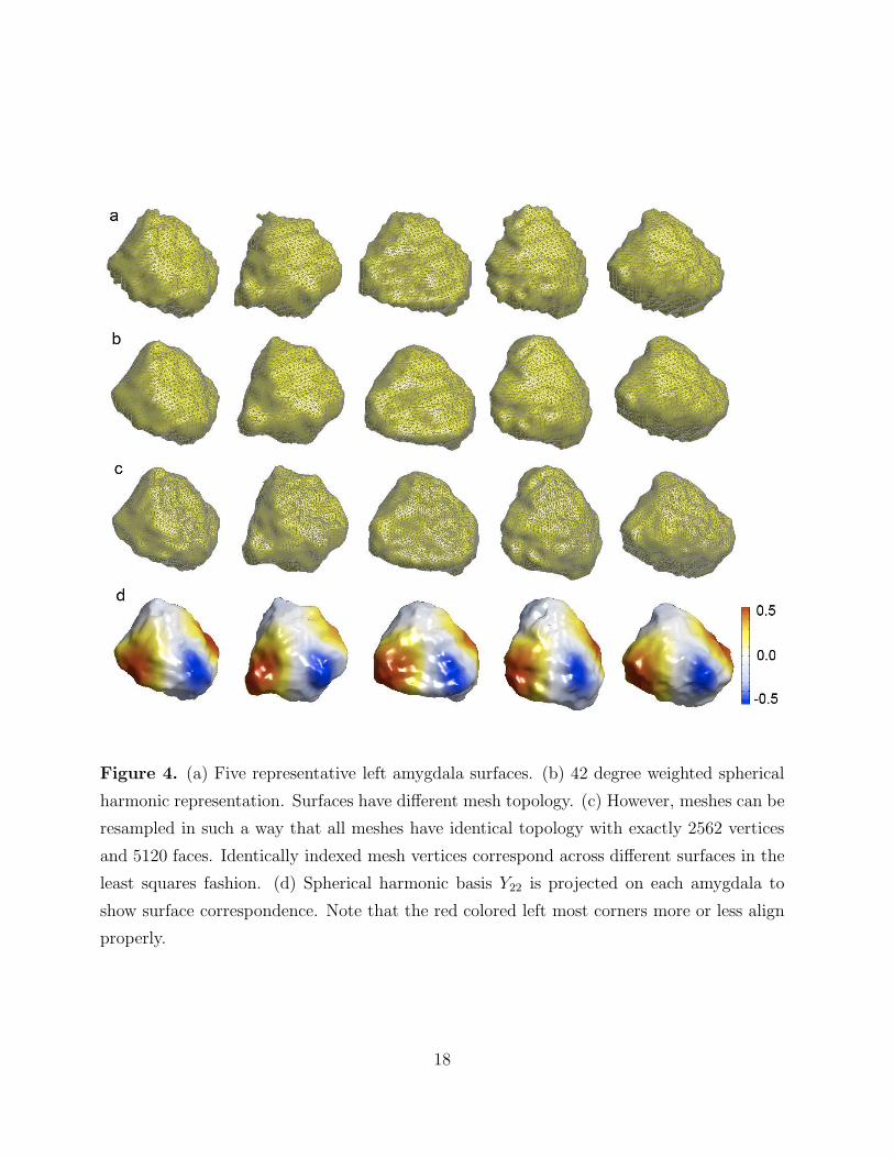
Figure 4. (a) Five representative left amygdala surfaces. (b) 42 degree weighted spherical

harmonic representation. Surfaces have different mesh topology. (c) However, meshes can be

resampled in such a way that all meshes have identical topology with exactly 2562 vertices

and 5120 faces. Identically indexed mesh vertices correspond across different surfaces in the

least squares fashion. (d) Spherical harmonic basis Y22 is projected on each amygdala to

show surface correspondence. Note that the red colored left most corners more or less align

properly.

18

Denote the surface coordinates corresponding to the i-th surface as pi. Then we have the

representation

pi(Ω) =k∑

l=0

l∑

m=−l

e−l(l+1)σf ilmYlm(Ω). (9)

There are total (k + 1)2 × 3 coefficients to be estimated. Assume there are total n surfaces,

the average surface p is given as

p =1

n

n∑

i=1

k∑

l=0

l∑

m=−l

e−l(l+1)σf ilmYlm. (10)

In our study, the average left and right amygdala templates are constructed by averaging

the spherical harmonic coefficients of all 24 control subjects. The template surfaces serve as

the reference coordinates for projecting the subsequent statistical parametric maps (Figure

7 and 8).

Validation. The methodology is validated in simulated surfaces where the ground truth is

exactly known. In order not to bias the result, we have used an intrinsic geometric method

using the Laplace-Beltrami eigenfunctions as a way to simulate surfaces with the known

ground truth (Levy and Inria-Alice, 2006). For the surface coordinates p, we have the

Laplace-Beltrami operator ∆ and its eigenfunctions ψj satisfying

ψj = λj∆ψj

where

0 = λ0 < λ1 ≤ λ2 ≤ · · · .

Then each surface can be represented as a linear combination of the Laplace-Beltrami eigen-

functions:

p =

∞∑

j=0

fjψj ,

where fj = 〈p, ψj〉. Note that low degree coefficients represent global shape features and

high degree coefficients represent high frequency local shape features. So by changing the

19

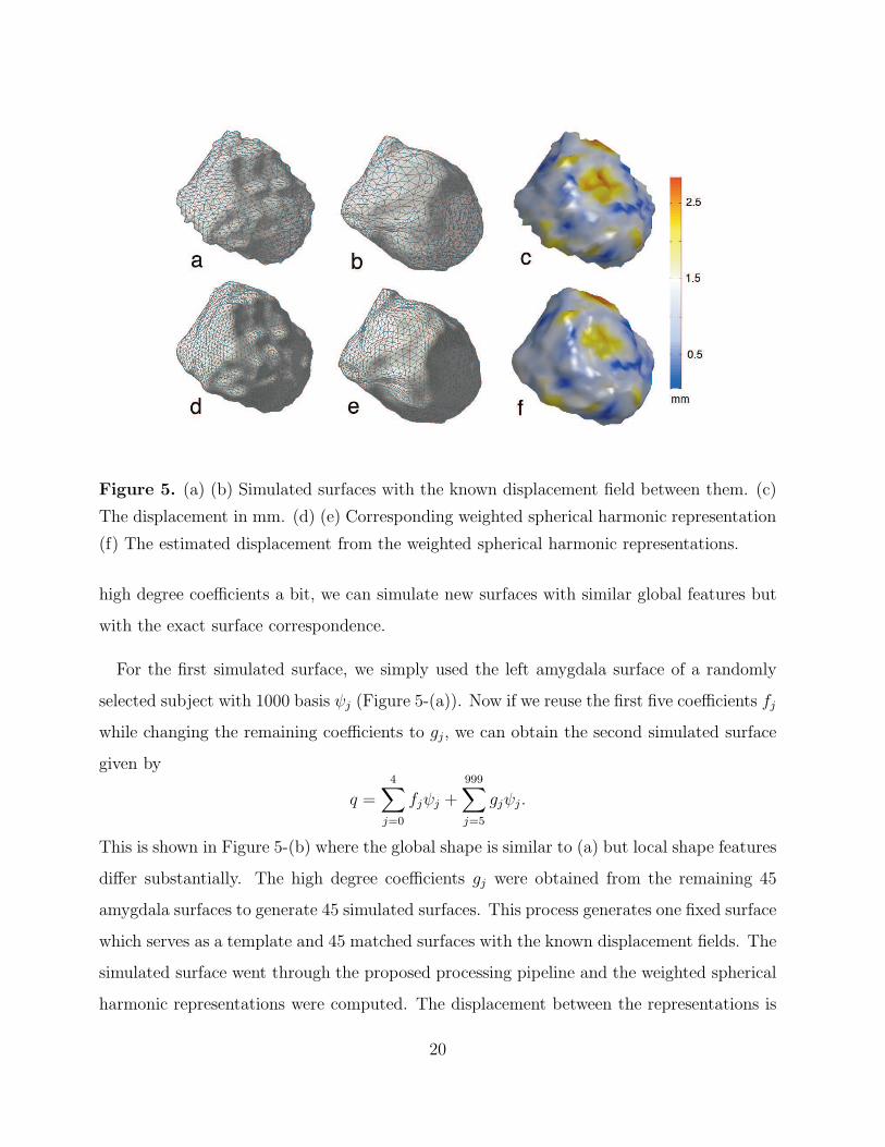
Figure 5. (a) (b) Simulated surfaces with the known displacement field between them. (c)

The displacement in mm. (d) (e) Corresponding weighted spherical harmonic representation

(f) The estimated displacement from the weighted spherical harmonic representations.

high degree coefficients a bit, we can simulate new surfaces with similar global features but

with the exact surface correspondence.

For the first simulated surface, we simply used the left amygdala surface of a randomly

selected subject with 1000 basis ψj (Figure 5-(a)). Now if we reuse the first five coefficients fj

while changing the remaining coefficients to gj, we can obtain the second simulated surface

given by

q =

4∑

j=0

fjψj +

999∑

j=5

gjψj .

This is shown in Figure 5-(b) where the global shape is similar to (a) but local shape features

differ substantially. The high degree coefficients gj were obtained from the remaining 45

amygdala surfaces to generate 45 simulated surfaces. This process generates one fixed surface

which serves as a template and 45 matched surfaces with the known displacement fields. The

simulated surface went through the proposed processing pipeline and the weighted spherical

harmonic representations were computed. The displacement between the representations is

20

given by the minimum distance (8). Figure 5-(f) shows the estimated displacement which

shows smoother pattern than the ground truth. This is expected since the ground truth

is the distance between noisy surfaces while the estimated displacement is the distance

between smooth functional representations. However, the pattern of estimation does follow

the pattern of the ground truth sufficiently well. In fact the mean relative error over each

surface is 0.116 ± 0.011.

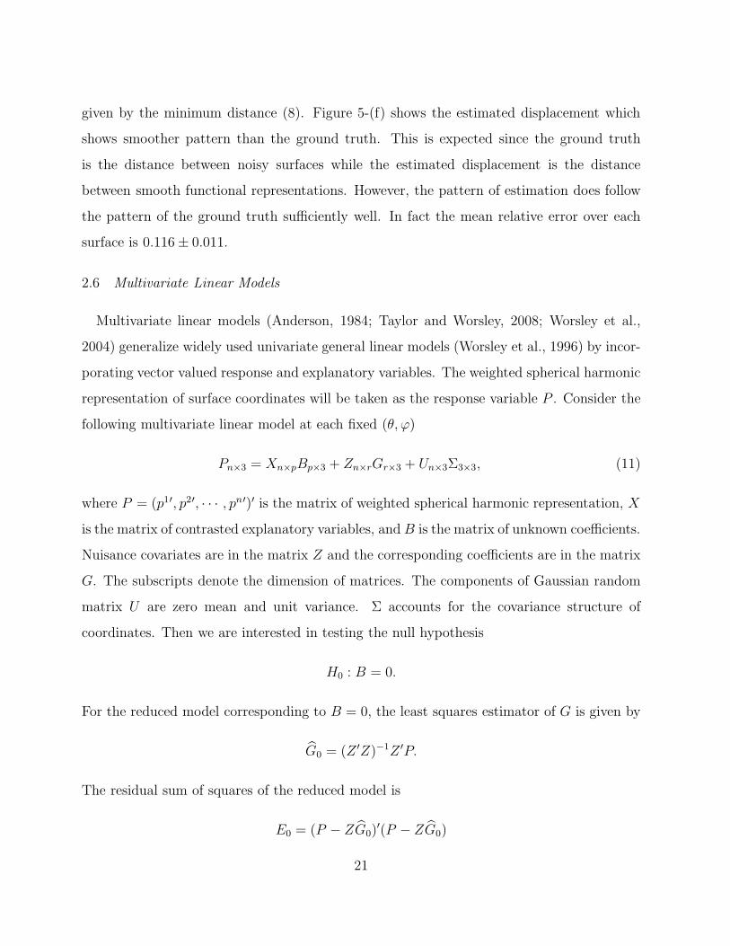
2.6 Multivariate Linear Models

Multivariate linear models (Anderson, 1984; Taylor and Worsley, 2008; Worsley et al.,

2004) generalize widely used univariate general linear models (Worsley et al., 1996) by incor-

porating vector valued response and explanatory variables. The weighted spherical harmonic

representation of surface coordinates will be taken as the response variable P . Consider the

following multivariate linear model at each fixed (θ, ϕ)

Pn×3 = Xn×pBp×3 + Zn×rGr×3 + Un×3Σ3×3, (11)

where P = (p1′, p2′, · · · , pn′)′ is the matrix of weighted spherical harmonic representation, X

is the matrix of contrasted explanatory variables, andB is the matrix of unknown coefficients.

Nuisance covariates are in the matrix Z and the corresponding coefficients are in the matrix

G. The subscripts denote the dimension of matrices. The components of Gaussian random

matrix U are zero mean and unit variance. Σ accounts for the covariance structure of

coordinates. Then we are interested in testing the null hypothesis

H0 : B = 0.

For the reduced model corresponding to B = 0, the least squares estimator of G is given by

G0 = (Z ′Z)−1Z ′P.

The residual sum of squares of the reduced model is

E0 = (P − ZG0)′(P − ZG0)

21

while that of the full model is

E = (P −XB − ZG)′(P −XB − ZG).

Note that G is different from G0 and estimated directly from the full model. By comparing

how large the residual E is against the residual E0, we can determine the significance of

coefficients B. However, since E and E0 are matrices, we take a function of eigenvalues of

EE−10 as a statistic. For instance, Lawley-Hotelling trace is given by the sum of eigenvalues

while Roy’s maximum rootR is the largest eigenvalue. In the case there is only one eigenvalue,

all these multivariate test statistics simplify to Hotelling’s T-sqaure statistic. The Hotelling’s

T-square statistic has been widely used in modeling 3D coordinates and deformations in

brain imaging (Cao and Worsley, 1999; Chung et al., 2001; Gaser et al., 1999; Joshi, 1998;

Thompson et al., 1997). The random field theory for Hotelling’s T-square statistic has been

available for a while (Cao and Worsley, 1999). However, the random field theory for the Roy’s

maximum root has not been developed until recently (Taylor and Worsley, 2008; Worsley

et al., 2004).

The inference for Roy’s maximum root is based on the Roy’s union-intersection principle

(Roy, 1953), which simplifies the multivariate problem to a univariate linear model. Let us

multiply an arbitrary constant vector ν3×1 on both sides of (11):

Pν = XBν + ZGν + UΣν. (12)

Obviously (12) is a usual univariate linear model with a Gaussian noise. For the univariate

testing on Bν = 0, the inference is based on the F statistic with p and n− p− r degrees of

freedom, denoted as Fν . Then Roy’s maximum root statistic can be defined as R = maxν Fν .

Now it is obvious that the usual random field theory can be applied in correcting for multiple

comparisons. The only trick is to increase the search space, in which we take the supreme

of the F random field, from the template surface to much higher dimension to account for

maximizing over ν as well.

22

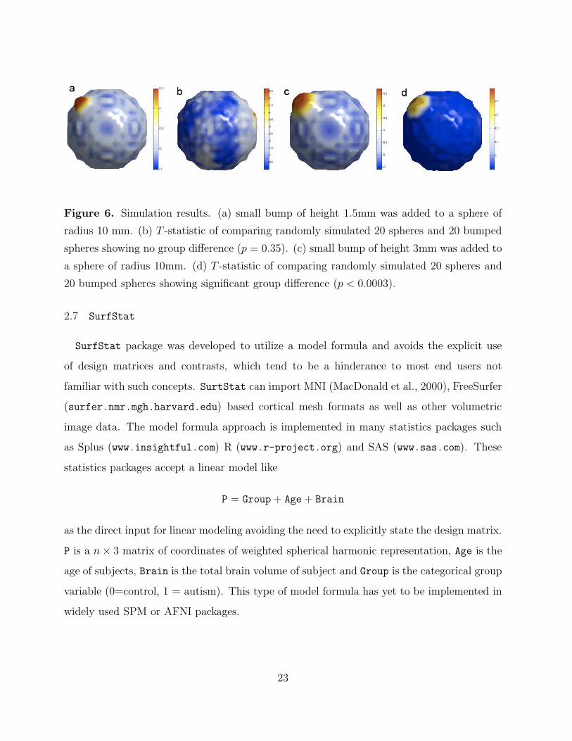
Figure 6. Simulation results. (a) small bump of height 1.5mm was added to a sphere of

radius 10 mm. (b) T -statistic of comparing randomly simulated 20 spheres and 20 bumped

spheres showing no group difference (p = 0.35). (c) small bump of height 3mm was added to

a sphere of radius 10mm. (d) T -statistic of comparing randomly simulated 20 spheres and

20 bumped spheres showing significant group difference (p < 0.0003).

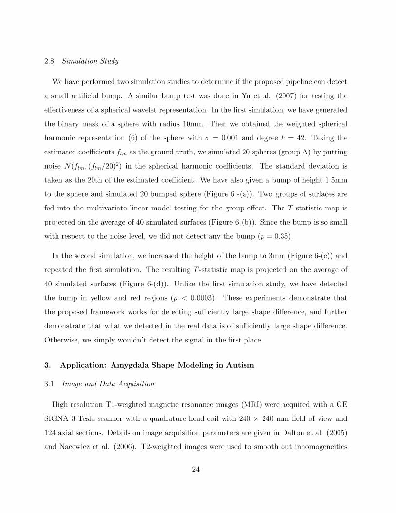
2.7 SurfStat

SurfStat package was developed to utilize a model formula and avoids the explicit use

of design matrices and contrasts, which tend to be a hinderance to most end users not

familiar with such concepts. SurtStat can import MNI (MacDonald et al., 2000), FreeSurfer

(surfer.nmr.mgh.harvard.edu) based cortical mesh formats as well as other volumetric

image data. The model formula approach is implemented in many statistics packages such

as Splus (www.insightful.com) R (www.r-project.org) and SAS (www.sas.com). These

statistics packages accept a linear model like

P = Group + Age + Brain

as the direct input for linear modeling avoiding the need to explicitly state the design matrix.

P is a n× 3 matrix of coordinates of weighted spherical harmonic representation, Age is the

age of subjects, Brain is the total brain volume of subject and Group is the categorical group

variable (0=control, 1 = autism). This type of model formula has yet to be implemented in

widely used SPM or AFNI packages.

23

2.8 Simulation Study

We have performed two simulation studies to determine if the proposed pipeline can detect

a small artificial bump. A similar bump test was done in Yu et al. (2007) for testing the

effectiveness of a spherical wavelet representation. In the first simulation, we have generated

the binary mask of a sphere with radius 10mm. Then we obtained the weighted spherical

harmonic representation (6) of the sphere with σ = 0.001 and degree k = 42. Taking the

estimated coefficients flm as the ground truth, we simulated 20 spheres (group A) by putting

noise N(flm, (flm/20)2) in the spherical harmonic coefficients. The standard deviation is

taken as the 20th of the estimated coefficient. We have also given a bump of height 1.5mm

to the sphere and simulated 20 bumped sphere (Figure 6 -(a)). Two groups of surfaces are

fed into the multivariate linear model testing for the group effect. The T -statistic map is

projected on the average of 40 simulated surfaces (Figure 6-(b)). Since the bump is so small

with respect to the noise level, we did not detect any the bump (p = 0.35).

In the second simulation, we increased the height of the bump to 3mm (Figure 6-(c)) and

repeated the first simulation. The resulting T -statistic map is projected on the average of

40 simulated surfaces (Figure 6-(d)). Unlike the first simulation study, we have detected

the bump in yellow and red regions (p < 0.0003). These experiments demonstrate that

the proposed framework works for detecting sufficiently large shape difference, and further

demonstrate that what we detected in the real data is of sufficiently large shape difference.

Otherwise, we simply wouldn’t detect the signal in the first place.

3. Application: Amygdala Shape Modeling in Autism

3.1 Image and Data Acquisition

High resolution T1-weighted magnetic resonance images (MRI) were acquired with a GE

SIGNA 3-Tesla scanner with a quadrature head coil with 240 × 240 mm field of view and

124 axial sections. Details on image acquisition parameters are given in Dalton et al. (2005)

and Nacewicz et al. (2006). T2-weighted images were used to smooth out inhomogeneities

24

in the inversion recovery-prepared images using FSL (www.fmrib.ox.ac.uk/fsl). Total 22

high functioning autistic and 24 normal control MRI were acquired. Subjects were all males

aged between 8 and 25 years. The Autism Diagnostic Interview-Revised (Lord et al., 1994)

was used for diagnoses by trained researchers K.M. Dalton and B.M. Nacewicz (Dalton et al.,

2005).

MRIs were first reoriented to the pathological plane for optimal comparison with anatomi-

cal atlases (Convit et al., 1999). Image contrast was matched by alignment of white and gray

matter peaks on intensity histograms. Manual segmentation was done by a trained expert

B.M. Nacewicz who has been blind to the diagnoses (Nacewicz et al., 2006). The manual

segmentation also involves refinement through plane-by-palne comparison with ex vivo atlas

sections (Mai et al., 1997). The reliability of the manual segmentation protocol was vali-

dated by two raters on 10 amygdale resulting in interclass correlation of 0.95 and the spatial

reliability (intersection over union) average of 0.84. Figure 1 shows the manual segmentation

of an amygdala in three different cross sections. The amygdala (AMY) was traced in detail

using various adjacent structures such as anterior commissure (AC), hippocampus (HIPP),

inferior horn of lateral ventricle (IH), optic radiations (OR), optic tract (OT), temporal lobe

white matter (TLWM) and tentorial notch (TN).

The total brain volume was also computed using an automated threshold-based connected

voxel search method, and manually edited afterwards to ensure proper removal of CSF, skull,

eye regions, brainstem and cerebellum using in-house software Spamalize (Oakes et al., 1999;

Rusch et al., 2001; Nacewicz et al., 2006). The brain volumes are 1224±128 and 1230±161

cm3 for autistic and control subjects. The volume difference is not significant (p = 0.89).

A subset of subjects (10 controls and 12 autistic) went through a face emotion recogni-

tion task consisting of showing 40 standardized pictures of posed facial expressions (8 each

of happy, angry and sad, and 16 neutral) (Dalton et al., 2005). Subjects were required to

press a button distinguishing neutral from emotional faces. The faces were black and white

pictures taken from the Karolinska Directed Emotional Faces set (Lundqvist et al., 1998).

25

The faces were presented using E-Prime software (www.pstnet.com) allowing for the mea-

surement of response time for each trial. iView system with a remote eye-tracking device

(SensoMotoric Instruments, www.smivision.com) was used at the same time to measure

gaze fixation duration on eyes and faces during the task. The system records eye movements

as the gaze position of the pupil over a certain length of time along with the amount of

time spent on any given fixation point. It has been hypothesized that subjects with autism

should exhibit diminished eye fixation duration relative to face fixation duration. If there is

no confusion, we will simply refer gaze fixation as the ratio of durations fixed on eyes over

faces. Note that this is a unitless measure. Our study enables us to show that abnormal

gaze fixation duration is correlated with amygdala shape in spatially localized regions.

3.2 Amygdala Volumetry

We have counted the number of voxels in amygdala segmentation and computed the vol-

ume of both left and right amygdale. The volumes for control subjects (n = 22) are left

1892 ± 173mm3, right 1883 ± 171mm3. The volumes for autistic subjects (n = 24) are left

1858 ± 182mm3, right 1862 ± 181mm3. The volume difference between the groups is not

statistically significant based on the two sample t-test (p = 0.52 for left and 0.69 for right).

The testing was done using SurfStat. Previous amygdala volumetry studies in autism have

been inconsistent (Aylward et al., 1999; Haznedar et al., 2000; Nacewicz et al., 2006; Pierce

et al., 2001; Schumann et al., 2004; Sparks et al., 2002). Aylward et al. (1999) and Pierce

et al. (2001) reported that significantly smaller amygdala volume in the autistic subjects

while Howard et al. (2000) and Sparks et al. (2002) reported larger volume. Haznedar et al.

(2000) and Nacewicz et al. (2006) found no volume difference. These inconsistency might

be due to the lack of control for brain size and age in statistical analysis (Schumann et al.,

2004).

26

3.3 Local Shape Difference

From the amygdala volumetry result, it is still not clear if shape difference might be

still present within amygdala. It is possible to have no volume difference while having

significant shape difference. So we have performed multivariate linear modeling on the

weighted spherical harmonic representation. We have tested the effect of group variable in

the model

P = 1 + Group,

which resulted in the threshold of 26.99 at α = 0.1. On the other hand the maximum

F statistic value is 13.55 (Figure 7 (a)). So we could not detect any shape difference in

the left amygdala. For the right amygdala, the threshold is 26.64 which is far larger than

the maximum F statistic value of 12.11. So again there is no statistically significant shape

difference in the right amygdala.

We have also tested the effect of Group variable while accounting for age and the total

brain volume in the SurfStat model form

P = Age + Brain + Group. (13)

The maximum F statistics are 14.77 (left) and 12.91 (right) while the threshold corresponding

to the α = 0.1 is 14.58 (left) and 14.61 (right). Hence, we still did not detect group difference

in the right amygdala (Figure 7-(d)) while there seems to be a bit weak group difference in

the left amygdala (Figure 7-(c)). However, they did not pass the α = 0.01 test so our result

is inconclusive. The enlarged area in Figure shows the average surface coordinate difference

(autism - control) in the region of the maximum F value.

Head circumference and brain enlargement are linked to autism (Dementieva et al., 2005;

Tager-Flusberg and Joseph, 2003) and thus the covariate Brain in the model (13) may

introduce a scaling related effect that was originally not present in the data. However, we

did not find significant brain volume difference between the groups (p = 0.89). The brain

size difference does not significantly compound our result. From figure 8, we can see that

27

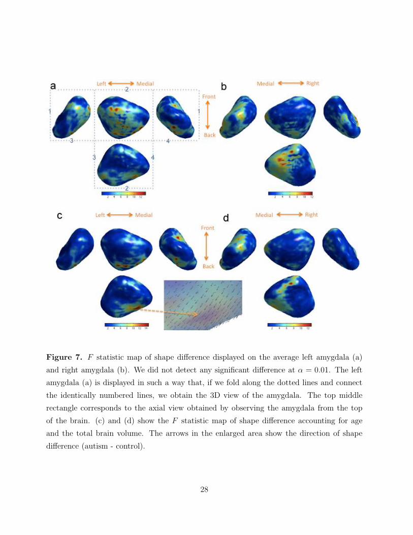
Figure 7. F statistic map of shape difference displayed on the average left amygdala (a)

and right amygdala (b). We did not detect any significant difference at α = 0.01. The left

amygdala (a) is displayed in such a way that, if we fold along the dotted lines and connect

the identically numbered lines, we obtain the 3D view of the amygdala. The top middle

rectangle corresponds to the axial view obtained by observing the amygdala from the top

of the brain. (c) and (d) show the F statistic map of shape difference accounting for age

and the total brain volume. The arrows in the enlarged area show the direction of shape

difference (autism - control).

28

the results between with and without covariating Brain are not much different (they are all

statistically insignificant). Therefore, Brain in the model mostly accounts for subject-specific

brain size difference rather than the group-specific brain size difference.

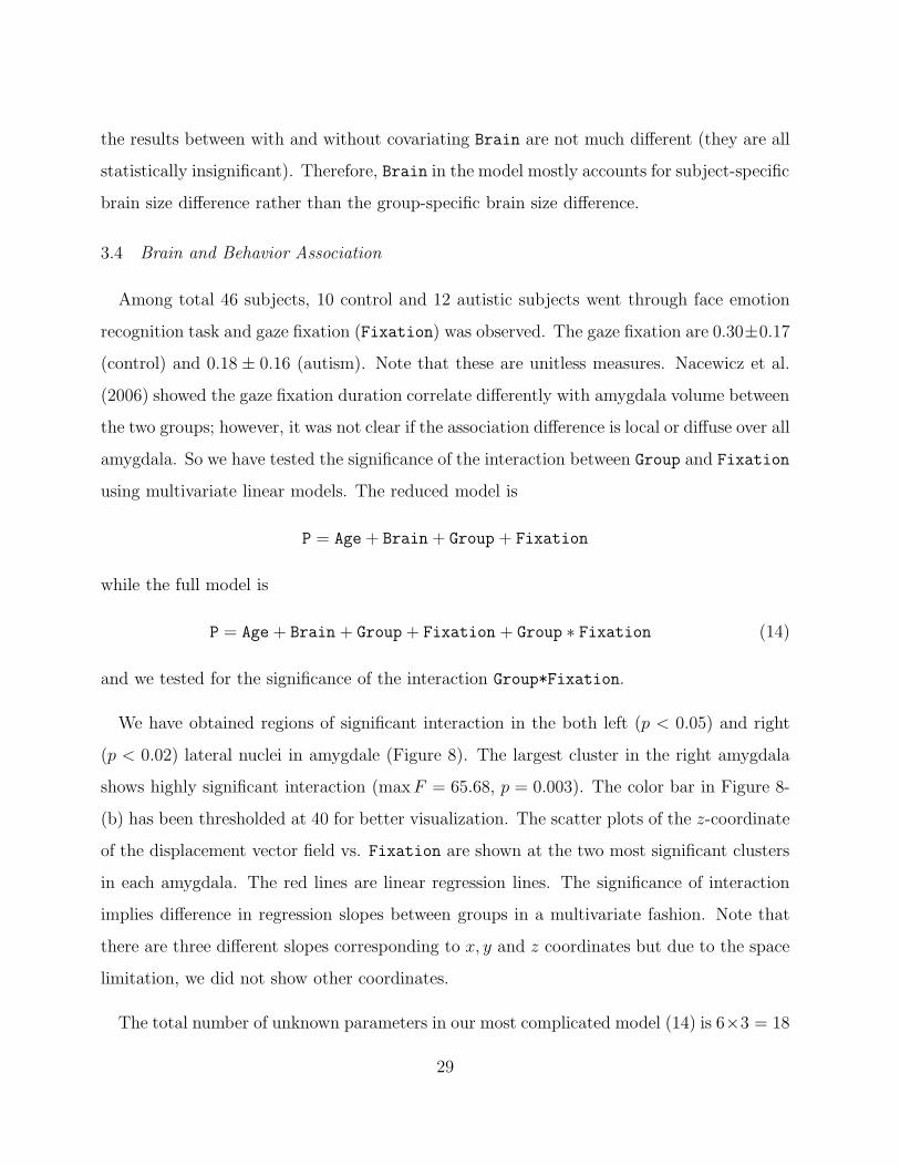
3.4 Brain and Behavior Association

Among total 46 subjects, 10 control and 12 autistic subjects went through face emotion

recognition task and gaze fixation (Fixation) was observed. The gaze fixation are 0.30±0.17

(control) and 0.18 ± 0.16 (autism). Note that these are unitless measures. Nacewicz et al.

(2006) showed the gaze fixation duration correlate differently with amygdala volume between

the two groups; however, it was not clear if the association difference is local or diffuse over all

amygdala. So we have tested the significance of the interaction between Group and Fixation

using multivariate linear models. The reduced model is

P = Age + Brain + Group + Fixation

while the full model is

P = Age + Brain + Group + Fixation + Group ∗ Fixation (14)

and we tested for the significance of the interaction Group*Fixation.

We have obtained regions of significant interaction in the both left (p < 0.05) and right

(p < 0.02) lateral nuclei in amygdale (Figure 8). The largest cluster in the right amygdala

shows highly significant interaction (maxF = 65.68, p = 0.003). The color bar in Figure 8-

(b) has been thresholded at 40 for better visualization. The scatter plots of the z-coordinate

of the displacement vector field vs. Fixation are shown at the two most significant clusters

in each amygdala. The red lines are linear regression lines. The significance of interaction

implies difference in regression slopes between groups in a multivariate fashion. Note that

there are three different slopes corresponding to x, y and z coordinates but due to the space

limitation, we did not show other coordinates.

The total number of unknown parameters in our most complicated model (14) is 6×3 = 18

29

Figure 8. F statistic map of interaction between group and gaze fixation. Red regions show

significant interaction for (a) left and (b) right amygdale. For better visualization, the color

bar for the right amygdala (b) has been thresholded at 40 since the maximum F statistics

at the largest cluster is 65.68 (p = 0.003). The scatter plots show the particular coordinate

of the displacement vector from the average surface vs. gaze fixation. The red lines are

regression lines.

30

including the constant terms. This is a large number of parameters to estimate if (14) was

a univariate linear model. However, in our multivariate setting, it is reasonable number

of parameters since we are also tripling the number of measurements as well. Note that

Roy’s maximum root statistic is based on maximizing an F -statistic with 1 and n − 1 − 5

degrees of freedom. Since the number of subjects is n = 22 + 24, we have the sufficient

degrees of freedom not to worry about the over-fitting problem. Unfortunately, practical

power approximation for Roy’s maximum root statistic does not exists although that of

Lawley-Hotelling trace is available (Barton and Cramer, 1989; O’Brien and Muller, 1993) so

the discussion of the parameter over-fitting is still an open statistical problem.

4. Discussion

Summary. The paper propose a unified multivariate linear modeling approach for a collec-

tion of binary neuroanatomical objects. The unified framework is applied to amygdala shape

analysis in autism. The surfaces of the binary objects are flattened using a new technique

based on heat diffusion. The coordinates of amygdala surfaces are smoothed and normal-

ized using the weighted spherical harmonic representation. The multivariate linear models

accounting for nuisance covariates are used using a newly developed SurfStat package.

Since surface data is inherently multivariate, traditionally Hotelling’s T-square approach

has been used on surface coordinates in a group comparison that can not account for nui-

sance covariates. On the other hand, the proposed multivariate linear model generalizes the

Hotelling’s T-square approach so that we can construct more complicated statistical mod-

els while accounting for additional covariates. The model formula based multivariate linear

modeling tool SurfStat has been developed for this purpose and publicly available. We have

applied the proposed methods to 22 autistic subjects to test if there is localized shape dif-

ference within an amygdala. We were able to localize regions, mainly in the right amygdala,

that shows differential association of gaze fixation with anatomy between the groups.

Anatomical Findings. Many MRI-based volumetric studies have shown inconsistent results

31

in determining if there are any abnormal amygdala volume difference (Aylward et al., 1999;

Howard et al., 2000; Haznedar et al., 2000; Pierce et al., 2001; Schumann et al., 2004; Sparks

et al., 2002; Nacewicz et al., 2006). These studies focus on the total volume difference of

amygdala obtained from MRI and was unable to determine if the volume difference is locally

focused within the subregions of amygdala or diffuse over all regions.

Although we did not detect statistically significant shape difference within amygdala at

0.01 level, we detected significant group difference of shape in relation to the gaze fixation

duration mostly in the both lateral nuclei (largest clusters in Figure 8). The lateral nucleus

receives information from the thalamus and cortex, and relay it to other subregions within

the amygdala. Our finding is consistent with literature that reports that autistic subjects

fail to activate the amygdala normally when processing emotional facial and eye expressions

(Baron-Cohen et al., 1999; Critchley et al., 2000; Barnea-Goraly et al., 2004). There are two

anatomical studies that additionally support our findings. A post-mortem study shows there

are increased neuron-packing density of the medial, cortical and central nuclei, and medial

and basal lateral nuclei of the amygdala in five autopsy cases (Courchesne, 1997). Fur-

ther, reduced fractional anisotropy is found in the temporal lobes approaching the amygdala

bilaterally in a diffusion tensor imaging study (Barnea-Goraly et al., 2004).

The inconsistent amygdala volumetry results seem to be caused by the local volume and

shape difference of the lateral nuclei that may or may not contribute to the total volume

of amygdala. Further diffusion tensor imaging studies on the white matter fiber tracts

connecting the lateral nuclei would shed a light on the abnormal nature of lateral nucleus of

the amygdala and its structural connection to other parts of the brain.

Methodological Limitations. There are few methodological limitations in our proposed

study. Surface flattening is based on tracing the streamline of the gradient of heat equilib-

rium. The proposed flattening technique is simple enough to be applied to various binary

objects. However, for the proposed flattening method to work, the binary object has to

be close to star-shape or convex. Theoretically, the solution to the Laplacian equation is

32

uniquely given and the heat gradient will never cross within the space between the inner and

outer boundaries. However, for more complex structures like cortical surfaces, the gradient

lines that correspond to neighboring nodes on the surface may fall within one voxel in the

volume, creating overlapping nonsmooth mapping to the sphere. The overlapping problem

can be avoided by subsampling the voxel grid in a much finer resolution but extending the

method to cortical surfaces is left as a future study.

Although the proposed framework of diffusion-based flattening and the weighted spherical

harmonic representation provide surface registration beyond the initial affine transforma-

tions, the accuracy is not high compared to other optimization based registration (Heimann

et al., 2005; Meier and Fisher, 2002; Styner et al., 2003). It is likely that the optimization

based methods will outperform our method. Although the comparative analysis against

these methods is the beyond the scope of the current paper, the simulation study in section

2.5 demonstrates the proposed method provides sufficiently good accuracy (relative error of

0.116 ± 0.011).

Although the proposed weighted spherical harmonic approach streamlines various image

processing tasks such as smoothing, representation and registration within a unified math-

ematical representation, we did not compare the performance with other available shape

representation techniques such as the medial representation (Pizer et al., 1999) and wavelets

(Yu et al., 2007). This is the beyond the scope of the current paper and requires an additional

comparative study.

Acknowledgment

The authors with to thank Martin A. Styner of the Department of Psychiatry and Computer

Science of the University of North Carolina at Chapel Hill and Shubing Wang of Merck for

various discussion on spherical harmonics. This research is supported in part by grant

1UL1RR025011 from the Clinical and Translational Science Award (CTSA) program of

the National Center for Research Resources, National Institutes of Health and WCU grant

33

through the department of Brain and Cognitive Sciences at Seoul National University.

References

Anderson, T. (1984). An Introduction to Multivariate Statistical Analysis. Wiley., 2nd.

edition.

Angenent, S., Hacker, S., Tannenbaum, A. and Kikinis, R. (1999). On the laplace-beltrami

operator and brain surface flattening. IEEE Transactions on Medical Imaging 18, 700–

711.

Ashburner, J., Hutton, C., Frackowiak, R. S. J., Johnsrude, I., Price, C. and Friston, K. J.

(1998). Identifying global anatomical differences: deformation-based morphometry. Hu-

man Brain Mapping 6, 348–357.

Aylward, E., Minshew, N., Goldstein, G., Honeycutt, N., Augustine, A., Yates, K., Bartra,

P. and Pearlson, G. (1999). Mri volumes of amygdala and hippocampus in nonmentally

retarded autistic adolescents and adults. Neurology 53, 2145–2150.

Barnea-Goraly, N., Kwon, H., Menon, V., Eliez, S., Lotspeich, L. and Reiss, A. (2004).

White matter structure in autism: preliminary evidence from diffusion tensor imaging.

Biological Psychiatry 55, 323–326.

Baron-Cohen, S., Ring, H., Wheelwright, S., Bullmore, E., Brammer, M., Sim-mons, A. and

Williams, S. (1999). Social intelligence in the normal and autistic brain: An fMRI study.

Eur J Neurosci 11, 1891–1898.

Barton, C. and Cramer, E. (1989). Hypothesis testing in multivariate linear models with

randomly missing data. Communications in Statistics-Simulation and Computation 18,

875–895.

Basser, P., Pajevic, S., Pierpaoli, C., Duda, J. and Aldroubi, A. (2000). In vivo tractography

using dt-mri data. Magnetic Resonance in Medicine 44, 625–632.

Blanco, M., Florez, M. and Bermejo, M. (1997). Evaluation of the rotation matrices in the

34

basis of real spherical harmonics. Journal of Molecular Structure: THEOCHEM 419,

19–27.

Brechbuhler, C., Gerig, G. and Kubler, O. (1995). Parametrization of closed surfaces for 3d

shape description. Computer Vision and Image Understanding 61, 154–170.

Bulow, T. (2004). Spherical diffusion for 3D surface smoothing. IEEE Transactions on

Pattern Analysis and Machine Intelligence 26, 1650–1654.

Cao, J. and Worsley, K. J. (1999). The detection of local shape changes via the geometry of

hotellings t2 fields. Annals of Statistics 27, 925–942.

Cates, J., Fletcher, P., Styner, M., Hazlett, H. and Whitaker, R. (2008). Particle-Based

Shape Analysis of Multi-Object Complexes. In Medical image computing and computer-

assisted intervention: MICCAI... International Conference on Medical Image Computing

and Computer-Assisted Intervention, volume 11, pages 477–485.

Chung, M., Dalton, K.M., L. S., Evans, A. and Davidson, R. (2007). Weighted Fourier rep-

resentation and its application to quantifying the amount of gray matter. IEEE Trans-

actions on Medical Imaging 26, 566–581.

Chung, M., Robbins, S., Dalton, K.M., D. R. A. A. and Evans, A. (2005). Cortical thickness

analysis in autism with heat kernel smoothing. NeuroImage 25, 1256–1265.

Chung, M., Worsley, K., Paus, T., Cherif, D., Collins, C., Giedd, J., Rapoport, J., and

Evans, A. (2001). A unified statistical approach to deformation-based morphometry.

NeuroImage 14, 595–606.

Chung, M., Worsley, K., Robbins, S., Paus, T., Taylor, J., Giedd, J., Rapoport, J. and Evans,

A. (2003). Deformation-based surface morphometry applied to gray matter deformation.

NeuroImage 18, 198–213.

Collins, D. L., Paus, T., Zijdenbos, A., Worsley, K. J., Blumenthal, J., Giedd, J. N.,

Rapoport, J. L. and Evans, A. C. (1998). Age related changes in the shape of tem-

poral and frontal lobes: An mri study of children and adolescents. Soc. Neurosci. Abstr.

24, 304.

Convit, A., McHugh, P., Wolf, O., de Leon, M., Bobinkski, M., De Santi, S., Roche, A. and

35

Tsui, W. (1999). Mri volume of the amygdala: a reliable method allowing separation

from the hippocampal formation. Psychiatry Res. 90, 113–123.

Courchesne, E. (1997). Brainstem, cerebellar and limbic neuroanatomical abnormalities in

autism. Current Opinion in Neurobiology 7, 269–278.

Critchley, H., Daly, E., Bullmore, E., Williams, S., T, V. A. and Robert-son, D. e. a. (2000).

The functional neuroanatomy of social behaviour: Changes in cerebral blood ow when

people with autistic disorder pro- cess facial expressions. Brain 123, 2203–2212.

Csernansky, J., Wang, L., Joshi, S., Tilak Ratnanather, J. and Miller, M. (2004). Com-

putational anatomy and neuropsychiatric disease: probabilistic assessment of variation

and statistical inference of group difference, hemispheric asymmetry, and time-dependent

change. NeuroImage 23, 56–68.

Dalton, K., Nacewicz, B., Johnstone, T., Schaefer, H., Gernsbacher, M., Goldsmith, H.,

Alexander, A. and Davidson, R. (2005). Gaze fixation and the neural circuitry of face

processing in autism. Nature Neuroscience 8, 519–526.

Dementieva, Y., Vance, D., Donnelly, S., Elston, L., Wolpert, C., Ravan, S., DeLong, G.,

Abramson, R., Wright, H. and Cuccaro, M. (2005). Accelerated head growth in early

development of individuals with autism. Pediatric neurology 32, 102–108.

Fischl, B. and Dale, A. (2000). Measuring the thickness of the human cerebral cortex from

magnetic resonance images. PNAS 97, 11050–11055.

Gaser, C., Volz, H.-P., Kiebel, S., Riehemann, S. and Sauer, H. (1999). Detecting structural

changes in whole brain based on nonlinear deformationsapplication to schizophrenia re-

search. NeuroImage 10, 107–113.

Gelb, A. (1997). The resolution of the gibbs phenomenon for spherical harmonics. Mathe-

matics of Computation 66, 699–717.

Gerig, G., Styner, M., Jones, D., Weinberger, D. and Lieberman, J. (2001). Shape analysis

of brain ventricles using spharm. In MMBIA, pages 171–178.

Gerig, G., Styner, M. and Szekely, G. (2004). Statistical shape models for segmentation

and structural analysis. In Proceedings of IEEE International Symposium on Biomedical

36

Imaging (ISBI), volume I, pages 467–473.

Golland, P., Grimson, W., Shenton, M. and Kikinis, R. (2001). Deformation analysis for

shape based classification. Lecture Notes in Computer Science pages 517–530.

Gu, X., Wang, Y., Chan, T., Thompson, T. and Yau, S. (2004). Genus zero surface conformal

mapping and its application to brain surface mapping. IEEE Transactions on Medical

Imaging 23, 1–10.

Haznedar, M., Buchsbaum, M., Wei, T., Hof, P., Cartwright, C. and Bienstock, C.A. Hol-

lander, E. (2000). Limbic circuitry in patients with autism spectrum disorders studied

with positron emission tomography and magnetic resonance imaging. American Journal

of Psychiatry 157, 1994–2001.

Heimann, T., Wolf, I., Williams, T. and Meinzer, H. (2005). 3D active shape models using

gradient descent optimization of description length. In Information Processing in Medical

Imaging, Lecture Notes in Computer Science, pages 566–577.

Homeier, H. and Steinborn, E. (1996). Some properties of the coupling coefficients of real

spherical harmonics and their relation to Gaunt coefficients. Journal of Molecular Struc-

ture: THEOCHEM 368, 31–37.

Howard, M., Cowell, P., Boucher, J., Broks, P., Mayes, A., Farrant, A. and Roberts, N.

(2000). Convergent neuroanatomical and behavioral evidence of an amygdala hypothesis

of autism. NeuroReport 11, 2931–2935.

Hurdal, M. K. and Stephenson, K. (2004). Cortical cartography using the discrete conformal

approach of circle packings. NeuroImage 23, S119S128.

Jones, D., Catani, M., Pierpaoli, C., Reeves, S., Shergill, S., O’Sullivan, M., Golesworthy,

P., McGuire, P., Horsfield, M., Simmons, A., Williams, S. and Howard, R. (2006). Age

effects on diffusion tensor magnetic resonance imaging tractography measures of frontal

cortex connections in schizophrenia. Human Brain Mapping 27, 230–238.

Joshi, S. (1998). Large Deformation Diffeomorphisms and Gaussian Random Fields for

Statistical Characterization of Brain Sub-Manifolds.

Joshi, S., Grenander, U. and Miller, M. (1997). The geometry and shape of brain sub-

37

manifolds. International Journal of Pattern Recognition and Artificial Intelligence: Spe-

cial Issue on Processing of MR Images of the Human 11, 1317–1343.

Joshi, S., Pizer, S., Fletcher, P., Yushkevich, P., Thall, A. and Marron, J. (2002). Multiscale

deformable model segmentation and statistical shape analysis using medial descriptions.

IEEE Transactions on Medical Imaging 21, 538–550.

Kelemen, A., Szekely, G. and Gerig, G. (1999). Elastic model-based segmentation of 3-d

neuroradiological data sets. IEEE Transactions on Medical Imaging 18, 828–839.

Khan, A., Chung, M. and Beg, M. (1999). Robust atlas-based brain segmentation using

multi-structure confidence-weighted registration. Lecture Notes on Computer Science

5762, 549–557.

Lazar, M., Weinstein, D., Tsuruda, J., Hasan, K., Arfanakis, K., Meyerand, M., Badie, B.,

Rowley, H., Haughton, V., Field, A., Witwer, B. and Alexander, A. (2003). White matter

tractography using tensor deflection. Human Brain Mapping 18, 306–321.

Lerch, J. P. and Evans, A. (2005). Cortical thickness analysis examined through power

analysis and a population simulation. NeuroImage 24, 163–173.

Leventon, M., Grimson, W. and Faugeras, O. (2000). Statistical shape influence in geodesic

active contours. In IEEE Conference on Computer Vision and Pattern Recognition, vol-

ume 1.

Levy, B. and Inria-Alice, F. (2006). Laplace-beltrami eigenfunctions towards an algorithm

that” understands” geometry. In IEEE International Conference on Shape Modeling and

Applications, 2006. SMI 2006, pages 13–13.

Lord, C., Rutter, M. and Couteur, A. (1994). Autism diagnostic interviewrevised: a revised

version of a diagnostic interview for caregivers of individuals with possible pervasive

developmental disorders. J Autism Dev Disord. pages 659–685.

Lorensen, W. and Cline, H. (1987). Marching cubes: A high resolution 3D surface construc-

tion algorithm. In Proceedings of the 14th annual conference on Computer graphics and

interactive techniques, pages 163–169.

Luders, E., Thompson, P.M., Narr, K., Toga, A., Jancke, L. and Gaser, C. (2006). A

38

curvature-based approach to estimate local gyrification on the cortical surface. NeuroIm-

age 29, 1224–1230.

Lundqvist, D., Flykt, A. and Ohman, A. (1998). Karolinska Directed Emotional Faces.

Department of Neurosciences, Karolinska Hospital, Stockholm, Sweden.

MacDonald, J., Kabani, N., Avis, D. and Evans, A. (2000). Automated 3-D extraction of

inner and outer surfaces of cerebral cortex from mri. NeuroImage 12, 340–356.

Mai, J., Assheuer, J. and Paxinos, G. (1997). Atlas of the Human Brain. Academic Press,

San Diego.

Meier, D. and Fisher, E. (2002). Parameter space warping: shape-based correspondence

between morphologically different objects. IEEE Transactions on Medical Imaging 21,

31–47.

Miller, M., Banerjee, A., Christensen, G., Joshi, S., Khaneja, N., Grenander, U. and Matejic,

L. (1997). Statistical methods in computational anatomy. Statistical Methods in Medical

Research 6, 267–299.

Miller, M., Massie, A., Ratnanather, J., Botteron, K. and Csernansky, J. (2000). Bayesian

construction of geometrically based cortical thickness metrics. NeuroImage 12, 676–687.

Nacewicz, B., Dalton, K., Johnstone, T., Long, M., McAuliff, E., Oakes, T., Alexander,

A. and Davidson, R. (2006). Amygdala volume and nonverbal social impairment in

adolescent and adult males with autism. Arch. Gen. Psychiatry 63, 1417–1428.

Nain, D., Styner, M., Niethammer, M., Levitt, J., Shenton, M., Gerig, G., Bobick, A. and

Tannenbaum, A. (2007). Statistical shape analysis of brain structures using spherical

wavelets. In IEEE Symposium on Biomedical Imaging ISBI.

Oakes, T., Koger, J. and Davidson, R. (1999). Automated whole-brain segmentation. Neu-

roImage 9, 237.

O’Brien, R. and Muller, K. (1993). Unified power analysis for t-tests through multivariate

hypotheses. Applied analysis of variance in behavioral science pages 297–344.

Pierce, K., Muller, R.A., A. J., Allen, G. and Courchesne, E. (2001). Face processing occurs

outside the fusiform ”face area” in autism: evidence from functional mri. Brain 124,

39

2059–2073.

Pizer, S., Fritsch, D., Yushkevich, P., Johnson, V. and Chaney, E. (1999). Segmentation, reg-

istration, and measurement of shape variation via image object shape. IEEE Transactions

on Medical Imaging 18, 851–865.

Qiu, A., and Miller, M. (2008). Multi-structure network shape analysis via normal surface

momentum maps. NeuroImage 42, 1430–1438.

Rojas, D., Smith, J., Benkers, T., Camou, S., Reite, M. and Rogers, S. (2000). Hippocampus

and amygdala volumes in paretns of children with autistic disorder. The Canadian Journal

of Statistics 28, 225–240.

Roy, S. (1953). On a heuristic method of test construction and its use in multivariate analysis.

Ann. Math. Statist. 24, 220–238.

Rusch, B., Abercrombie, H., Oakes, T., Schaefer, S. and Davidson, R. (2001). Hippocampal

morphometry in depressed patients and control subjects: relations to anxiety symptoms.

Biological Psychiatry 50, 960–964.

Saad, Z., Reynolds, R., Argall, B., Japee, S. and Cox, R. (2004). Suma: an interface for

surface-based intra-and inter-subject analysis with afni. In IEEE International Sympo-

sium on Biomedical Imaging (ISBI), pages 1510–1513.

Schumann, C., Hamstra, J., Goodlin-Jones, B., Lotspeich, L., Kwon, H., Buonocore, M.,

Lammers, C., Reiss, A. and Amaral, D. (2004). The amygdala is enlarged in children

but not adolescents with autism; the hippocampus is enlarged at all ages. Journal of

Neuroscience 24, 6392–6401.

Shen, L. and Chung, M. (2006). Large-scale modeling of parametric surfaces using spherical

harmonics. In Third International Symposium on 3D Data Processing, Visualization and

Transmission (3DPVT).

Shen, L., Ford, J., Makedon, F. and Saykin, A. (2004). surface-based approach for classifi-

cation of 3d neuroanatomical structures. Intelligent Data Analysis 8, 519–542.

Sparks, B., Friedman, S., Shaw, D., Aylward, E., Echelard, D., Artru, A., Maravilla, K.,

Giedd, J., Munson, J., Dawson, G. and Dager, S. (2002). Brain structural abnormalities

40

in young children with autism spectrum disorder. Neurology 59, 184–192.

Styner, M., Gerig, G., Joshi, S. and Pizer, S. (2003). Automatic and robust computation

of 3d medial models incorporating object variability. International Journal of Computer

Vision 55, 107–122.

Styner, M., Oguz, I., Xu, S., Brechbuhler, C., Pantazis, D., Levitt, J., Shenton, M. and Gerig,

G. (2006). Framework for the statistical shape analysis of brain structures using spharm-

pdm. In Insight Journal, Special Edition on the Open Science Workshop at MICCAI.

Tager-Flusberg, H. and Joseph, R. (2003). Identifying neurocognitive phenotypes in autism.

Philosophical Transactions: Biological Sciences 358, 303–314.

Taylor, J. and Worsley, K. (2008). Random fields of multivariate test statistics, with appli-

cations to shape analysis. Annals of Statistics page in press.

Thompson, P., Giedd, J., Woods, R., MacDonald, D., Evans, A. and Toga, A. (2000).

Growth patterns in the developing human brain detected using continuum-mechanical

tensor mapping. Nature 404, 190–193.

Thompson, P. and Toga, A. (1996). A surface-based technique for warping 3-dimensional

images of the brain. IEEE Transactions on Medical Imaging 15.

Thompson, P. M., MacDonald, D., Mega, M. S., Holmes, C. J., Evans, A. C. and Toga,

A. W. (1997). Detection and mapping of abnormal brain structure with a probabilistic

atlas of cortical surfaces. J. Comput. Assist. Tomogr. 21, 567–581.

Timsari, B. and Leahy, R. (2000). An optimization method for creating semi-isometric flat

maps of the cerebral cortex. In The Proceedings of SPIE, Medical Imaging.

Worsley, K., Marrett, S., Neelin, P., Vandal, A., Friston, K. and Evans, A. (1996). A unified

statistical approach for determining significant signals in images of cerebral activation.

Human Brain Mapping 4, 58–73.

Worsley, K., Taylor, J., Tomaiuolo, F. and Lerch, J. (2004). Unified univariate and multi-

variate random field theory. NeuroImage 23, S189–195.

Yezzi, A. and Prince, J. (2001). A PDE approach for measuring tissue thickness. In IEEE

Computer Society Conference on Computer Vision and Pattern Recognition (CVPR).

41

Yu, P., Grant, P., Qi, Y., Han, X., Segonne, F., Pienaar, R., Busa, E., Pacheco, J., Makris, N.,

Buckner, R. et al. (2007). Cortical Surface Shape Analysis Based on Spherical Wavelets.

IEEE Transactions on Medical Imaging 26, 582.

Appendix

We illustrate SurfStat package by showing the step-by-step command lines for multivariate

linear models used in the study. The detailed description of the SurfStat package can be

found in www.stat.uchicago.edu/∼worsley/surfstat. The SurfStat is a general purpose

surface analysis package and it requires additional codes and for amygdala specific analysis.

The additional codes can be found in

www.stat.wisc.edu/∼mchung/research/amygdala.

Given an amygdala mesh surf, which is, for instance, given as a structured array of the

form

surf =

vertices: [1270x3 double]

faces: [2536x3 double]

the amygdala flattening algorithm will generate the corresponding unit sphere mesh sphere

that has identical topology as surf. The weighted spherical harmonic representation P with

degree k = 42 and the bandwidth σ = 0.001 is computed from

>[P,coeff]=SPHARMsmooth(surf,sphere,42,0.001);

The coordinates of the weighted spherical harmonic representation have been read into

an array of size 46 (subjects) × 2562 (vertices) × 3 (coordinates) P. Brain size (brain), age

(age), group variable (group) are read into 46 (subjects) × 1 vectors. The group categorical

variable consists of strings ’control’ and ’autism’. We now convert these to terms that

can be combined into a multivariate linear model as follows:

42

>Brain = term( brain );

>Age = term( age );

>Group = term ( group );

>Group

autism control

---------------

0 1

0 1

1 0

1 0

. .

. .

. .

To test the effect of group, the linear model of the from P = 1 + Group is fitted by

>E = SurfStatLinMod( P,1 + Group, Avg );

where Avg is the average surface obtained from the weighted spherical harmonic representa-

tion.

We specify a group contrast and calculate the T -statistic:

>contrast = Group.autism - Group.control

contrast =

-1

-1

1

1

.

.

.

LM = SurfStatT( E, contrast );

43

LM.t gives the vector of 2562 T -statistic values for all mesh vertices. Instead of using the

contrast and T -statistic, we can test the effect of group variable using the F -statistic as well:

>E0 = SurfStatLinMod( P,1 );

>LM = SurfStatF( E,E0 );

E0 contains the information about the sum of squared residual of the reduced model P = 1

in E0.SSE while E contains that of the full model P = 1 + Group. Based on the ratio of the

sum of squared residuals, SurfStatF computes the F -statistics. To display the F -statistic

value on top of the average surface, we use FigureOrigami( Avg, LM.t ) which produces

Figure 7.

We can determine the random field based thresholding corresponding to α = 0.01 level:

>resels = SurfStatResels(LM);

>stat_threshold( resels, length(LM.t),1,LM.df,0.01,[],[],[],LM.k)

peak_threshold =

26.9918

resels computes the resels of the random field and peak threshold is the threshold corre-

sponding to 0.1 level.

We can construct a more complicated model that includes the brain size and age as

covariates:

>E0 = SurfStatLinMod(P,Age+Brain);

>E = SurfStatLinMod(P,Age+Brain+Group,Avg);

>LM = SurfStatF(E,E0);

LM.t contains the F -statistic of the significance of group variable while accounting for age

and brain size. We can also test for interaction between gaze fixation Fixation and group

variable:

44

>E0=SurfStatLinMod(P,Age+Brai +Group+Fixation);

>E=SurfStatLinMod(P,Age+Brain+Group+Fixation+Group*Fixation,Avg);

>LM=SurfStatF(E,E0);

45