General methods for generating phase-shifting interferometry algorithms

General methods for generatingphase-shifting interferometry algorithms

D. W. Phillion

Two completely independent systematic approaches for designing algorithms are presented. One ap-proach uses recursion rules to generate a new algorithm from an old one, only with an insensitivity tomore error sources. The other approach uses a least-squares method to optimize the noise performanceof an algorithm while constraining it to a desired set of properties. These properties might includeinsensitivity to detector nonlinearities as high as a certain power, insensitivity to linearly varying laserpower, and insensitivity to some order to the piezoelectric transducer voltage ramp with the wrong slope.A noise figure of merit that is valid for any algorithm is also derived. This is crucial for evaluatingalgorithms and is what is maximized in the least-squares method. This noise figure of merit is a certainaverage over the phase because in general the noise sensitivity depends on it. It is valid for bothquantization noise and photon noise. The equations that must be satisfied for an algorithm to beinsensitive to various error sources are derived. A multivariate Taylor-series expansion in the distor-tions is used, and the time-varying background and signal amplitudes are expanded in Taylor series intime. Many new algorithms and families of algorithms are derived. © 1997 Optical Society of America

Key words: Phase measuring, phase determining, phase shift, interferometry.

1. Introduction

Phase-shifting interferometry has been a major evo-lutionary step in interferometer design.1,2 It pro-vides a method to measure the phase u tounprecedented accuracy, better than ly1000. To dophase-shifting interferometry, one takes a conven-tional interferometer and varies the phase of the ref-erence wave linearly with time. This can beaccomplished by several methods, but the one mostcommonly used is translation of a mirror with a pi-ezoelectric transducer ~PZT!. The result is a chang-ing interference pattern. The interference patternis usually measured at a number of equally spacedtimes. Each of these interference patterns is calleda frame. The jth intensity frame measured at thetime tj has the form

Ij~x, y! 5 A~x, y! 1 B~x, y!cos@2pntj 1 u~x, y!#, (1.1)

where x,y is the position, A~x,y! is the background,B~x,y! is the amplitude, and u~x,y! is the phase that

The author is with the Advanced Microtechnology Program,Lawrence Livermore National Laboratory, P.O. Box 808, Liver-more, California 94550.

Received 3 September 1996.0003-6935y97y318098-18$10.00y0© 1997 Optical Society of America

8098 APPLIED OPTICS y Vol. 36, No. 31 y 1 November 1997

is to be measured. The frequency n is determined byhow fast the phase of the reference wave is changing.

The phase differences 2pn~tj11 2 tj! are called thephase steps and are usually chosen to be equal.There are three unknowns A, B, and u that can bedetermined from three measurements. Each mea-surement gives an equation that is linear in the vari-ables A, B exp~iu!, and B exp~2iu!. For threeframes, the resulting matrix equation can be invertedto obtain a solution of the form:

B exp~iu! 5 (j

rjIj 5 (j

@Re~rj!Ij 1 i Im~rj!Ij#, (1.2)

where Re and Im denote the real and imaginaryparts, respectively, and rj are obtained from the ma-trix inversion. Equivalently,

u 5 tan213(jIm~rj!Ij

(j

Re~rj!Ij4 . (1.3)

Appendix A gives the general solution for a three-frame algorithm with equal phase steps. Table 1lists several specific three-point algorithms.

If there were no errors, a three-frame algorithmwould be sufficient for determining u with unlimitedaccuracy. In reality the PZT motion is not exact, theCCD detector is not truly linear, and there are un-

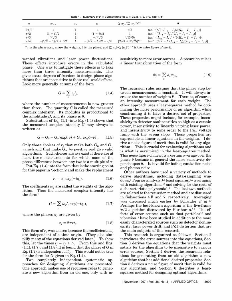
Table 1. Summary of P 5 3 Algorithms for a 5 2py3, py2, py3, and py4a

a w21 w0 w1 ¥ wjuy~¥ uwju2!1y2 u

2py3 1 1 1 =3 tan21@=3 ~I21 2 I1!y~2I0 2 I1 2 I21!#py2 ~1 1 i!y2 1 ~1 2 i!y2 1 tan21 @~I21 2 I1!y~2I0 2 I1 2 I21!#py3 iy=3 1 2iy=3 =~3y5! tan21$@I21 2 I1#y@=3~2I0 2 I1 2 I21!#%py4 2~=2 2 1!y2 1 iy2 1 2~=2 2 1!y2 2 iy2 @2y~5 1 3=2!#1y2 tan21@~=2 2 1!~I21 2 I1!y~2I0 2 I1 2 I21!#

aa is the phase step, w are the weights, u is the phase, and u¥ wjuy~¥ uwju2!1y2 is the noise figure of merit.

wanted vibrations and laser power fluctuations.These effects introduce errors in the calculatedphase. One way to mitigate these effects is to takemore than three intensity measurements. Thisgives extra degrees of freedom to design phase algo-rithms that are insensitive to these real-world effects.Look more generally at sums of the form

G 5 (j

rjIj, (1.4)

where the number of measurements is now greaterthan three. The quantity G is called the measuredcomplex intensity. Its modulus is proportional tothe amplitude B, and its phase is u.

Substitution of Eq. ~1.1! into Eq. ~1.4! shows thatthe measured complex intensity G may always bewritten as

G 5 G0 1 G1 exp~iu! 1 G2 exp~2iu!. (1.5)

Only those choices of rj that make both G0 and G2

vanish and that make G1 be positive real give validalgorithms. Such choices always exist if there are atleast three measurements for which none of thephase differences between any two is a multiple of p.

Put Eq. ~1.4! into the form that is the starting pointfor this paper in Section 2 and make the replacement

rj 5 wj exp~2iwj!. (1.6)

The coefficients wj are called the weights of the algo-rithm. Thus the measured complex intensity hasthe form1

G 5 (j

wjIj exp~2iwj!, (1.7)

where the phases wj are given by

wj 5 2pntj. (1.8)

This form of rj was chosen because the coefficients wjare independent of a time origin. ~They also sim-plify many of the equations derived later.! To showthis, let the times tj 5 tj 1 t0. From this and Eqs.~1.1!, ~1.7!, and ~1.8!, it is found that the phase of G inEq. ~1.7! is independent of t0. This would not be truefor the form for G given in Eq. ~1.4!.

Two completely independent systematic ap-proaches for designing algorithms are presented.One approach makes use of recursion rules to gener-ate a new algorithm from an old one, only with in-

sensitivity to more error sources. A recursion rule isa linear transformation of the form

w# j 5 (k

akwj1k. (1.9)

The recursion rules assume that the phase step be-tween measurements is constant. It will always in-crease the number of weights P. There is, of course,an intensity measurement for each weight. Theother approach uses a least-squares method for opti-mizing the noise performance of an algorithm whileconstraining it to have a desired set of properties.These properties might include, for example, insen-sitivity to detector nonlinearities as high as a certainpower, insensitivity to linearly varying laser power,and insensitivity to some order to the PZT voltageramp with the wrong slope. These properties areexpressible as linear equations in the weights. I de-rive a noise figure of merit that is valid for any algo-rithm. This is crucial for evaluating algorithms andis what is maximized in the least-squares method.This noise figure of merit is a certain average over thephase u because in general the noise sensitivity de-pends upon u. It is valid for both quantization noiseand photon noise.

Other authors have used a variety of methods toderive algorithms, including data-sampling win-dows,3 Fourier analysis,4,5 least squares,6,7 averagingwith existing algorithms,8 and solving for the roots ofa characteristic polynomial.9 The last two methodsare related to the recursion method and are discussedin Subsections 4.F and 7, respectively. Averagingwas discussed much earlier by Schwider et al.10

Perhaps the best-known algorithm is the five-framepy2 algorithm discovered by Hariharan.11 The ef-fects of error sources such as dust particles10 andvibration12 have been studied in addition to the moreeasily characterized sources such as detector nonlin-earity, laser power drift, and PZT distortion that arethe main subjects of this research.

This research is organized as follows: Section 2introduces the error sources into the equations, Sec-tion 3 derives the equations that the weights mustsatisfy for the algorithm to be insensitive to variouserror sources, Section 4 derives the recursion rela-tions for generating from an old algorithm a newalgorithm that has additional desired properties, Sec-tion 5 derives a noise figure of merit that is valid forany algorithm, and Section 6 describes a least-squares method for designing optimal algorithms.

1 November 1997 y Vol. 36, No. 31 y APPLIED OPTICS 8099

2. General Considerations

Find the weights wj and times tj so that the phase ofa signal I~t! is the same as the phase of the sum,

G 5 (j

wjIj exp~2iwj!. (2.1)

Here each Ij is an intensity measurement and wj ishow much the optical path difference has increased atthe time of the jth measurement. Increasing themeasurement path in the interferometer increases w.

Obtain the fundamental equations that theweights for any valid algorithm must satisfy. Letthe measured values Ij at the times tj be given by

Ij 5 A0 1 B0 cos~2pn0tj 1 u!, (2.2)

where A0 and B0 are constants. For finding the con-ditions upon the weights so that the phase of themeasured complex intensity G is always u when n0 5n, use the identity cos~x! 5 @exp~ix! 1 exp~2ix!#y2 toobtain

G 5 G0 1 G1~n0!exp~1iu! 1 G2~n0!exp~2iu!, (2.3)

where

G0 5 A0 (j

wj exp~2iwj!,

G1~n0! 512

B0 (j

wj exp~2pin0tj 2 iwj!,

G2~n0! 512

B0 (j

wj exp~22pin0tj 2 iwj!. (2.4)

When n0 5 n, these equations simplify to

G1 5B0

2 (j

wj,

G0 5 A0 (j

wj exp~2iwj!,

G2 5B0

2 (j

wj exp~22iwj!. (2.5)

For the phase of G to always be u when n0 5 n, G1

must be positive real and both G2 and G0 must bezero. This gives the fundamental set of equations:

(j

wj 5 positive real, (2.6a)

(j

wj exp~2iwj! 5 0, (2.6b)

(j

wj exp~22iwj! 5 0. (2.6c)

Now that the fundamental equations are derived,distortions, detector nonlinearitities, background andsignal drift, and vibration are included in a moregeneral formalism. All these effects are put into thesignal I~t!, which is assumed to have the form

I~t! 5 x~t! 1 a2@x~t!#2 1 a3@x~t!#3 1 · · · , (2.7)


where

x~t! 5 A~t! 1 B~t! cosH2pFn0t 1g2

2~n0t!

2

1g3

3~n0t!

3 1 · · · G 1 u 1 DuvibJ, (2.8)

where

Duvib 5vL

cεvib cos~2pnvibt 1 uvib!. (2.9)

The coefficients a2, a3, and so forth represent qua-dratic, cubic, and other nonlinearities in the detector.The vibration has amplitude εvib, frequency nvib, andphase uvib. Also, vL is the optical angular frequency.A~t! is the background amplitude, and B~t! is thesignal amplitude. The background and signal am-plitudes are represented by the power series:

A~t! 5 A0 1 A1t 1 A2t2 1 · · · ,

B~t! 5 B0 1 B1t 1 B2t2 1 · · · . (2.10)

The fringe visibility uB~t!yA~t!u can never exceed 1, ofcourse. The source frequency n0 may differ from thereference frequency n as determined by the PZT mo-tion. This gives rise to what is variously called first-order distortion, linear distortion, or slope error andis given by

ε 5n0

n2 1. (2.11)

The second-order distortion g2 is defined so that theinstantaneous source frequency is n0~1 1 g2n0t!.Fictitiously putting the distortions into the signalresults in mathematical simplifications.

Substituting Eqs. ~2.7!, ~2.8!, ~2.9!, and ~2.10! intoEq. ~2.1! gives an extremely complicated general ex-pression for G. The presence of detector nonlineari-ties causes G to have the more complicated form:

G 5 (n52`

1`

Gn~n0, $gj%, $aj%, $Aj%, $Bj%,

$εvib, nvib, uvib%!exp~inu!, (2.12)

where sets of coefficients have been enclosed in curlybrackets. If the detector is linear, there are onlyterms for n 5 21, 0, and 11. In Section 3, I workwith only one error source at a time. For each errorsource, G has a different form.

The times tj are assumed to be equally spaced sothat 2pntj 5 ja, where a is the phase step. Theindex j is either an integer or a half integer whichvaries in integer steps from a negative half-integervalue to the oppositely signed positive half-integervalue.

The weights are symmetric if there exists a numberN such that wj 5 wN2j. They are Hermitian if thereexists an N such that wj 5 wN2j*, where the asteriskdenotes the complex conjugate. For instance, the

weights wj 5 1, 2, 1 for j 5 1, 2, 3 are symmetricbecause wj 5 w42j.

The effect of finite measurement integration time13

is omitted for brevity and simplicity. Including thiseffect did not change the equations to make variouserror sources vanish. For distortions, what was un-changed by finite integration time was the set ofequations for making all distortions vanish as high assome order.

3. Error Sources

A. Piezoelectric Transducer Distortions

In the presence of distortions, the components of Gare given by

G0 5 A0 (j

wj exp~2iwj!,

G1~n0, g2, . . . ! 5B0

2 (j

wj expH2piFn0tj 1g2

2~ntj!

2

1g3

2~ntj!

3 1 . . . G 2 iwjJ ,

G2~n0, g2, . . . ! 5B0

2 (j

wj expH22piFn0tj 1g2

2~ntj!

2

1g3

2~ntj!

3 1 . . . G 2 iwjJ , (3.1)

where n0 5 ~1 1 ε!n and G 5 G0 1 G1 exp~iu! 1 G2

exp~2iu!. I assume that when ε 5 0 and g2 5 g35 . . . 5 0, G2 5 G0 5 0 and G1 is positive real.Equations ~3.1! may be obtained as discussed in Sec-tion 2. Notice that G0 does not depend upon ε and sois zero for any ε. If it were possible to make G2 zero,the only phase error would be due to G1 not beingpositive real. The phase of G1 would introduce aphase error that would be independent of u. How-ever, for phase-shift interferometry, any phase errorthat is independent of u is unimportant. Thus I needonly try to make G2 be nearly zero for small distor-tions.

Suppose that there is only slope error. G2~n0!may then be expanded in a Taylor series about n0 5n. I derive the equations that the weights of an al-gorithm must satisfy to cause the first ND 1 1 termsin this Taylor series to vanish. The rth order deriv-ative of G2~n0! with respect to n0 evaluated at n0 5 nis given by

]r

]n0r G2~n0!U

n05n

5B0~2ia!r

2 (j

jrwj exp~22iwj!. (3.2)

Here a is the phase step, and the j ranges from 2~P 21!y2 to ~P 2 1!y2 in integer steps. An algorithm hasa distortion insensitivity index of ND if the deriva-tives in Eqs. ~3.1! vanish for r 5 1, 2, . . . , ND.

A sum rule is defined to have either the form ¥ wjexp~ijx! 5 0 or the form expressible by the set ofequations ¥ wj exp~ijx! 5 0, ¥j1wj exp~ijx! 5 0, . . . ,¥ jRwj exp~ijx! 5 0. A sum rule is preserved by the

recursion relations that will be studied in Section 4.Here R is some positive integer, and x is some com-plex number. Because any valid algorithm mustsatisfy ¥ wj exp~22iwj! 5 0, it can be seen that thisequation together with the equations obtained bydemanding that the partial derivatives in Eq. ~3.2!vanish for r 5 1, 2, . . . , R form a sum rule of thesecond type with x 5 22a.

Now evaluate the mixed partial derivative withrespect to the various orders of distortion

]I1J1K1· · ·

]n0I]g2

J]g3K · · ·

G2~n0, g2, g3, . . . !Un05ng25g35· · ·50

5 _ ( jI12J13K1· · ·wj exp~22iwj!, (3.3)

where the constant _ is given by

_ 5B0

2 F22pi1 S a

2pD1GIF22pi

2 S a

2pD2GJ

3 F22pi3 S a

2pD3GK

· · · . (3.4)

If an algorithm has a distortion insensitivity index ofND, all such mixed partial derivatives with I 1 2J 13K 1 . . . # ND vanish.

B. Background and Signal Drift

Suppose that signal and background drift are presentbut that there are no PZT distortions or detectornonlinearities. The components of G then have theform

G0~A! 5 (j

wj~A0 1 A1tj 1 A2tj2 1 · · · !exp~2iwj!,

G1~B! 512 (

jwj~B0 1 B1tj 1 B2tj

2 1 · · · !,

G2~B! 512 (

jwj~B0 1 B1tj 1 B2tj

2 1 · · · !exp~22iwj!.

(3.5)

This equation may be derived as discussed in Section2.

Find what is required for the algorithm to be in-sensitive to signal drift A~t!. Because 2pntj 5 ja, therequirement that the Br term in G2 vanish is

(j

jrwj exp~22iwj! 5 0. (3.6)

This condition is already familiar for making PZTdistortions vanish, and it is possible to generalize therule about insensitivity to a mixture of PZT distor-tions: For the mixed partial derivative of order Iwith respect to the first-order distortion ε, order Jwith respect to the second-order distortion g, order Kwith respect to the third-order distortion, etc. to van-ish in the presence of Sth-order signal drift, the sums¥ jrwj exp~22iwj! must vanish for r 5 0, 1, . . . , S 1I 1 2J 1 3K 1 . . . . If the algorithm has distortion


insensitivity index ND, all such terms for which S 1I 1 2J 1 3K 1 . . . # ND vanish.

However, signal drift will never happen by itselfunless it is contrived. Changing laser power causesboth the background and the signal to change. Ifthere is no ambient light and no dark current, theywill change proportionately. The requirement thatthe Ar term vanish is that

(j

jrwj exp~2iwj! 5 0. (3.7)

The algorithm is insensitive to background drift toorder R if Eq. ~3.7! is satisfied for r 5 1, 2, . . . , R.This set of equations along with the equation ¥ wjexp~2iwj! in Eqs. ~2.6! form a sum rule that is pre-served by the recursion rules discussed in Section 4.

C. Detector Nonlinearity

Assume that the only error source is detector nonlin-earity. Then, as discussed in Section 2, it can beshown that G has the form

G 5 (j

wj (n51

`

an (k

(lSnklDAn2k2lSB

2Dk1l

3 exp@i~k 2 l !~u 1 wj!#exp~2iwj!. (3.8)

The double sum over k and l is over all nonnegativeinteger k and l that satisfy k 1 l # n. Define theindex m 5 k 2 l 2 1. Suppose that an 5 0 for n .N. Then G has the form

G 5 (m52N21

N21

Km~A, B, $an%!F(j

wj exp~imwj!G3 exp@i~m 1 1!u#. (3.9)

I am not concerned with the exact form of the func-tions Km~A, B, $an%!. For the algorithm to be insen-sitive to these detector nonlinearities, the coefficientof exp~iu! must be nonzero, but the coefficients ofexp~iku! vanish for k Þ 11. This requires that

(j

wj exp~imwj! 5 0 (3.10)

for m 5 2N 2 1, 2N, . . . , N 2 1 but m Þ 0. If wj 5j 2ppyq, where the integers p and q are relativelyprime, the largest that N can be is q 2 2. If N equalsq 2 1, the sum with m 5 2N 2 1 requires that ¥ wj5 0 because ~2N 2 1!a 5 22pp and exp~2i2pp! 5 1.However, a valid algorithm is required to have ¥ wjbe positive real.

D. Vibrations

Assume there is a vibration of amplitude εvib, fre-quency nvib, and phase uvib. The sum G is given by

G 5 (n52`

1`

Gn~εvib, nvib, uvib!exp~inu!, (3.11)


as discussed in Section 2. To obtain the form of theGn, start with

I~t! 5 A 1 B cosF2pnt 1 u 1vL

cεvib cos~2pnvibt 1 uvib!G.

(3.12)

This may be obtained from Eqs. ~2.7!–~2.10! throughthe assumption that there is no slope error or otherdistortion and no detector nonlinearity and that A~t!and B~t! are constants. Define

X~t! 5 2pnt 1 u,

Y~t! 5 ~vLεvibyc! cos~2pnvibt 1 uvib!. (3.13)

The argument of the cosine function in Eq. ~3.12! isX 1 Y. Use the trigonometric identity cos~X 1 Y! 5cos X cos Y 2 sin X sin Y. Now Y 5 x cos~y!, wherex 5 vLεvibyc and y 5 2pnvibt 1 uvib. Assume that theamplitude of the vibration is small that only terms ashigh as first order in x need to be kept. Then cos Y '1 and sin Y ' x cos~y!. Substituting these resultsinto Eq. ~3.12! gives

I~t! < A 1 B$cos~2pnt 1 u! 2 x sin~2pnt 1 u!cos@Y~t!#%.

(3.14)

The approximation sign is omitted in what follows.Now substitute Eq. ~3.14! into Eqs. ~3.1! and use wj 52pntj to obtain

G1 5B2 (

jwj@1 1 ix cos~Yj!#,

G0 5 A (j

wj exp~2iwj!,

G2 5B2 (

jwj@1 2 ix cos~Yj!#exp~22iwj!, (3.15)

where Yj 5 Y~tj!. Now use Eqs. ~2.6!, which are theequations any valid algorithm must satisfy, to sim-plify this to

G1 5B2 (

jwj 1

B2 (

jwj@ix cos~Yj!#,

G0 5 0,

G2 5B2 (

jwj@2ix cos~Yj!#exp~22iwj!. (3.16)

Replace cos~Yj! by @exp~iYj! 1 exp~2iYj!#y2 to obtain

G1 5B2 (

jwj 1

ix2

@exp~iuvib!G1~1! 1 exp~2iuvib!G1

~2!#,

G0 5 0,

G2 52ix2

@exp~iuvib!G2~1! 1 exp~2iuvib!G2

~2!#, (3.17)

where

G1~1! 5

B2 (

jwj exp~i2pnvibtj!,

G1~2! 5

B2 (

jwj exp~2i2pnvibtj!,

G2~1! 5

B2 (

jwj exp~i2pnvibtj!exp~22iwj!,

G2~2! 5

B2 (

jwj exp~2i2pnvibtj!exp~22iwj!. (3.18)

Eqs. ~2.4! give G1~n0!, G0~n0!, and G2~n0!, and

G1~1! 5 G1~n 1 nvib!,

G1~2! 5 G1~n 2 nvib!,

G2~1! 5 G2~n 2 nvib!,

G2~2! 5 G2~n 1 nvib!. (3.19)

Substituting Eqs. ~3.19! into Eqs. ~3.17!, the finalresult is obtained for the components of G:

G1 5B2 (

jwj 1

i2 SvLεvib

c D@exp~iuvib!G1~n 1 nvib!

1 exp~2iuvib!G1~n 2 nvib!#,

G0 5 0,

G2 52i2 SvLεvib

c D@exp~iuvib!G2~n 2 nvib!

1 exp~2iuvib!G2~n 1 nvib!#, (3.20)

where the substitution for x have also been made.Now I evaluate the phase error du, which is a func-

tion of εvib, nvib, uvib, and u. Assume that the weightsare Hermitian. ~All the algorithms I consider in thispaper are Hermitian.! For Hermitian weights,G1~n0! and G2~n0! are purely real for all n0. For thisproblem I therefore have

G 5 ~G1 1 dG1!exp~iu! 1 ~G2 1 dG2!exp~2iu!, (3.21)

where G1 and G2 are both real but dG1 and dG2 arenot. Assuming that dG1 and dG2 are small andG2 5 0, the phase error is given by

du 5 HIm@dG1 1 dG2 exp~22iu!#

G1J . (3.22)

Evaluating this gives

du 5 du1 1 du2, (3.23)

where

du1 5 SvLεvib

2cG1D@cos~uvib!G1~n 1 nvib!

1 cos~uvib!G1~n 2 nvib!#,

du2 5 2SvLεvib

2cG1D@cos~2u 1 uvib!G2~n 1 nvib!

1 cos~2u 2 uvib!G2~n 2 nvib!#. (3.24)

Note that the part of the phase error du1 is indepen-dent of the phase u, but the part du2 is oscillatory in2u. If ~du!2 is averaged over all u, it is found that

~du!2 5 ~du1!2 1 ~du2!2, (3.25)

where the overbar indicates the average over u. If Ithen average over the phase of the vibration,

^~du!2& 5 ^~du1!2& 1 ^~du2!2&, (3.26)

where the angular brackets indicate an average overthe phase of the vibration. The individual terms inEq. ~3.26! are given by

^~du1!2& 512 SvLεvib

2cG1D2

@G1~n 1 nvib! 1 G1~n 2 nvib!#2,

^~du2!2& 512 SvLεvib

2cG1D2

$@G2~n 1 nvib!#2 1 @G2~n 2 nvib!#

2% .

(3.27)

For phase-shift interferometry, I am unconcernedwith a phase shift that is independent of the phase u.Because du1 is independent of the phase u, it is onlythe du2 term that contributes to the noise. An algo-rithm is said to be relatively insensitive to a vibrationof frequency nvib if both G2~n 1 nvib! and G2~n 2 nvib!vanish and absolutely insensitive if the sum G1~n 1nvib! 1 G1~n 2 nvib! vanishes as well. Thus, to berelatively insensitive, G2~n0! must vanish for n0 5 n6 nvib. G2~n0! is given in Eqs. ~2.4!. This is theequation that the weights must satisfy to be rela-tively insensitive to a vibration of a particular fre-quency regardless of its phase.

High-frequency wide-bandwidth vibrations and la-ser power fluctuations are equivalent to noise. It isnot possible to design an algorithm that is insensitiveto these effects. If one cannot eliminate these errorsources sufficiently, the best approach is then to takethe measurements as rapidly as possible. One wayto do this with three measurements is described byWizinowich.14

4. Recursion Rules

A. Introduction

Recursion rules can be used to generate from oldalgorithms new algorithms that have additional de-sired properties. A recursion rule generates a newalgorithm from an existing one through a transfor-mation of the form w# j 5 ¥ akwj1k, where the sum isover k. The phase step a is unchanged. Recursionrules commute. Applying a recursion rule does notcause any property to be lost that is expressible asa sum rule that has either the form ¥ wj exp~ijx! 50 or the form of the set of equations ¥ wj exp~ijx! 50, ¥ j1wj exp~ijx! 5 0, ¥ j2wj exp~ijx! 5 0, . . . , ¥ jRwjexp~ijx! 5 0, for some positive integer R. Here x is


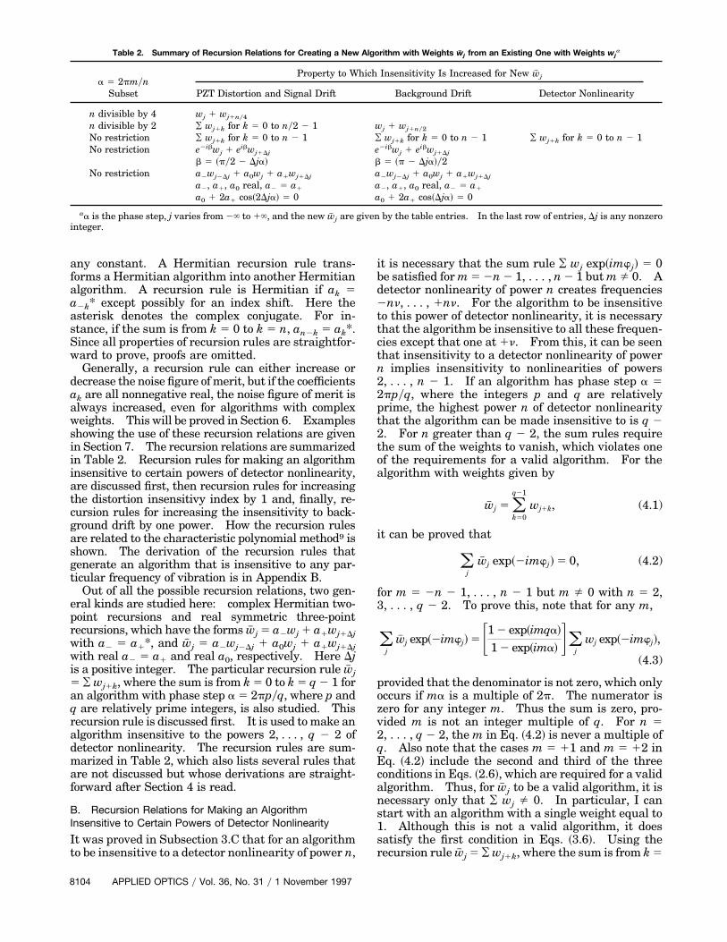
Table 2. Summary of Recursion Relations for Creating a New Algorithm with Weights w# j from an Existing One with Weights wja

a 5 2pmynSubset

Property to Which Insensitivity Is Increased for New w# j

PZT Distortion and Signal Drift Background Drift Detector Nonlinearity

n divisible by 4 wj 1 wj1ny4

n divisible by 2 ¥ wj1k for k 5 0 to ny2 2 1 wj 1 wj1ny2

No restriction ¥ wj1k for k 5 0 to n 2 1 ¥ wj1k for k 5 0 to n 2 1 ¥ wj1k for k 5 0 to n 2 1No restriction e2ibwj 1 eibwj1Dj e2ibwj 1 eibwj1Dj

b 5 ~py2 2 Dja! b 5 ~p 2 Dja!y2No restriction a2wj2Dj 1 a0wj 1 a1wj1Dj a2wj2Dj 1 a0wj 1 a1wj1Dj

a2, a1, a0 real, a2 5 a1 a2, a1, a0 real, a2 5 a1

a0 1 2a1 cos~2Dja! 5 0 a0 1 2a1 cos~Dja! 5 0

aa is the phase step, j varies from 2` to 1`, and the new w# j are given by the table entries. In the last row of entries, Dj is any nonzerointeger.

any constant. A Hermitian recursion rule trans-forms a Hermitian algorithm into another Hermitianalgorithm. A recursion rule is Hermitian if ak 5a2k* except possibly for an index shift. Here theasterisk denotes the complex conjugate. For in-stance, if the sum is from k 5 0 to k 5 n, an2k 5 ak*.Since all properties of recursion rules are straightfor-ward to prove, proofs are omitted.

Generally, a recursion rule can either increase ordecrease the noise figure of merit, but if the coefficientsak are all nonnegative real, the noise figure of merit isalways increased, even for algorithms with complexweights. This will be proved in Section 6. Examplesshowing the use of these recursion relations are givenin Section 7. The recursion relations are summarizedin Table 2. Recursion rules for making an algorithminsensitive to certain powers of detector nonlinearity,are discussed first, then recursion rules for increasingthe distortion insensitivy index by 1 and, finally, re-cursion rules for increasing the insensitivity to back-ground drift by one power. How the recursion rulesare related to the characteristic polynomial method9 isshown. The derivation of the recursion rules thatgenerate an algorithm that is insensitive to any par-ticular frequency of vibration is in Appendix B.

Out of all the possible recursion relations, two gen-eral kinds are studied here: complex Hermitian two-point recursions and real symmetric three-pointrecursions, which have the forms w# j 5 a2wj 1 a1wj1Djwith a2 5 a1*, and w# j 5 a2wj2Dj 1 a0wj 1 a1wj1Djwith real a2 5 a1 and real a0, respectively. Here Djis a positive integer. The particular recursion rule w# j5 ¥ wj1k, where the sum is from k 5 0 to k 5 q 2 1 foran algorithm with phase step a 5 2ppyq, where p andq are relatively prime integers, is also studied. Thisrecursion rule is discussed first. It is used to make analgorithm insensitive to the powers 2, . . . , q 2 2 ofdetector nonlinearity. The recursion rules are sum-marized in Table 2, which also lists several rules thatare not discussed but whose derivations are straight-forward after Section 4 is read.

B. Recursion Relations for Making an AlgorithmInsensitive to Certain Powers of Detector Nonlinearity

It was proved in Subsection 3.C that for an algorithmto be insensitive to a detector nonlinearity of power n,


it is necessary that the sum rule ¥ wj exp~imwj! 5 0be satisfied for m 5 2n 2 1, . . . , n 2 1 but m Þ 0. Adetector nonlinearity of power n creates frequencies2nn, . . . , 1nn. For the algorithm to be insensitiveto this power of detector nonlinearity, it is necessarythat the algorithm be insensitive to all these frequen-cies except that one at 1n. From this, it can be seenthat insensitivity to a detector nonlinearity of powern implies insensitivity to nonlinearities of powers2, . . . , n 2 1. If an algorithm has phase step a 52ppyq, where the integers p and q are relativelyprime, the highest power n of detector nonlinearitythat the algorithm can be made insensitive to is q 22. For n greater than q 2 2, the sum rules requirethe sum of the weights to vanish, which violates oneof the requirements for a valid algorithm. For thealgorithm with weights given by

w# j 5 (k50

q21

wj1k, (4.1)

it can be proved that

(j

w# j exp~2imwj! 5 0, (4.2)

for m 5 2n 2 1, . . . , n 2 1 but m Þ 0 with n 5 2,3, . . . , q 2 2. To prove this, note that for any m,

(j

w# j exp~2imwj! 5 F1 2 exp~imqa!

1 2 exp~ima! G(jwj exp~2imwj!,

(4.3)

provided that the denominator is not zero, which onlyoccurs if ma is a multiple of 2p. The numerator iszero for any integer m. Thus the sum is zero, pro-vided m is not an integer multiple of q. For n 52, . . . , q 2 2, the m in Eq. ~4.2! is never a multiple ofq. Also note that the cases m 5 11 and m 5 12 inEq. ~4.2! include the second and third of the threeconditions in Eqs. ~2.6!, which are required for a validalgorithm. Thus, for w# j to be a valid algorithm, it isnecessary only that ¥ wj Þ 0. In particular, I canstart with an algorithm with a single weight equal to1. Although this is not a valid algorithm, it doessatisfy the first condition in Eqs. ~3.6!. Using therecursion rule w# j 5 ¥ wj1k, where the sum is from k 5

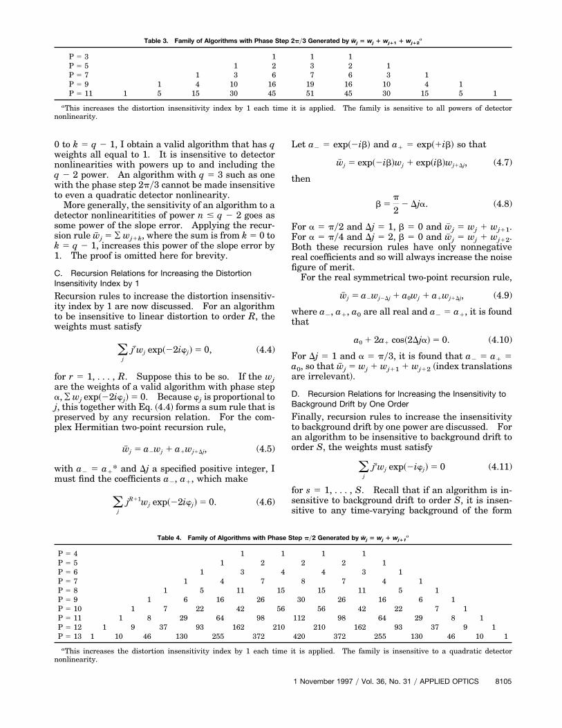
Table 3. Family of Algorithms with Phase Step 2py3 Generated by w# j 5 wj 1 wj11 1 wj12a

P 5 3 1 1 1P 5 5 1 2 3 2 1P 5 7 1 3 6 7 6 3 1P 5 9 1 4 10 16 19 16 10 4 1P 5 11 1 5 15 30 45 51 45 30 15 5 1

aThis increases the distortion insensitivity index by 1 each time it is applied. The family is sensitive to all powers of detectornonlinearity.

0 to k 5 q 2 1, I obtain a valid algorithm that has qweights all equal to 1. It is insensitive to detectornonlinearities with powers up to and including theq 2 2 power. An algorithm with q 5 3 such as onewith the phase step 2py3 cannot be made insensitiveto even a quadratic detector nonlinearity.

More generally, the sensitivity of an algorithm to adetector nonlinearitities of power n # q 2 2 goes assome power of the slope error. Applying the recur-sion rule w# j 5 ¥ wj1k, where the sum is from k 5 0 tok 5 q 2 1, increases this power of the slope error by1. The proof is omitted here for brevity.

C. Recursion Relations for Increasing the DistortionInsensitivity Index by 1

Recursion rules to increase the distortion insensitiv-ity index by 1 are now discussed. For an algorithmto be insensitive to linear distortion to order R, theweights must satisfy

(j

jrwj exp~22iwj! 5 0, (4.4)

for r 5 1, . . . , R. Suppose this to be so. If the wjare the weights of a valid algorithm with phase stepa, ¥ wj exp~22iwj! 5 0. Because wj is proportional toj, this together with Eq. ~4.4! forms a sum rule that ispreserved by any recursion relation. For the com-plex Hermitian two-point recursion rule,

w# j 5 a2wj 1 a1wj1Dj, (4.5)

with a2 5 a1* and Dj a specified positive integer, Imust find the coefficients a2, a1, which make

( jR11wj exp~22iwj! 5 0. (4.6)
j
Let a2 5 exp~2ib! and a1 5 exp~1ib! so that

w# j 5 exp~2ib!wj 1 exp~ib!wj1Dj, (4.7)

then

b 5p

22 Dja. (4.8)

For a 5 py2 and Dj 5 1, b 5 0 and w# j 5 wj 1 wj11.For a 5 py4 and Dj 5 2, b 5 0 and w# j 5 wj 1 wj12.Both these recursion rules have only nonnegativereal coefficients and so will always increase the noisefigure of merit.

For the real symmetrical two-point recursion rule,

w# j 5 a2wj2Dj 1 a0wj 1 a1wj1Dj, (4.9)

where a2, a1, a0 are all real and a2 5 a1, it is foundthat

a0 1 2a1 cos~2Dja! 5 0. (4.10)

For Dj 5 1 and a 5 py3, it is found that a2 5 a1 5a0, so that w# j 5 wj 1 wj11 1 wj12 ~index translationsare irrelevant!.

D. Recursion Relations for Increasing the Insensitivity toBackground Drift by One Order

Finally, recursion rules to increase the insensitivityto background drift by one power are discussed. Foran algorithm to be insensitive to background drift toorder S, the weights must satisfy

(j

jswj exp~2iwj! 5 0 (4.11)

for s 5 1, . . . , S. Recall that if an algorithm is in-sensitive to background drift to order S, it is insen-sitive to any time-varying background of the form

Table 4. Family of Algorithms with Phase Step py2 Generated by w# j 5 wj 1 wj11a

P 5 4 1 1 1 1P 5 5 1 2 2 2 1P 5 6 1 3 4 4 3 1P 5 7 1 4 7 8 7 4 1P 5 8 1 5 11 15 15 11 5 1P 5 9 1 6 16 26 30 26 16 6 1P 5 10 1 7 22 42 56 56 42 22 7 1P 5 11 1 8 29 64 98 112 98 64 29 8 1P 5 12 1 9 37 93 162 210 210 162 93 37 9 1P 5 13 1 10 46 130 255 372 420 372 255 130 46 10 1

aThis increases the distortion insensitivity index by 1 each time it is applied. The family is insensitive to a quadratic detectornonlinearity.


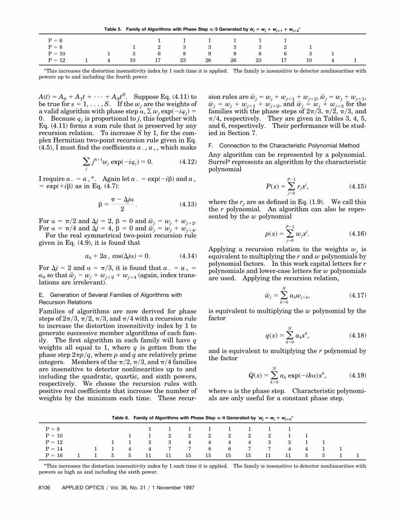
Table 5. Family of Algorithms with Phase Step py3 Generated by w# j 5 wj 1 wj11 1 wj12a

P 5 6 1 1 1 1 1 1P 5 8 1 2 3 3 3 3 2 1P 5 10 1 3 6 8 9 9 8 6 3 1P 5 12 1 4 10 17 23 26 26 23 17 10 4 1

aThis increases the distortion insensitivity index by 1 each time it is applied. The family is insensitive to detector nonlinearities withpowers up to and including the fourth power.

A~t! 5 A0 1 A1t 1 . . . 1 AStS. Suppose Eq. ~4.11! tobe true for s 5 1, . . . , S. If the wj are the weights ofa valid algorithm with phase step a, ¥ wj exp~2iwj! 50. Because wj is proportional to j, this together withEq. ~4.11! forms a sum rule that is preserved by anyrecursion relation. To increase S by 1, for the com-plex Hermitian two-point recursion rule given in Eq.~4.5!, I must find the coefficients a2, a1, which make

(j

jS11wj exp~2iwj! 5 0. (4.12)

I require a2 5 a1*. Again let a2 5 exp~2ib! and a1

5 exp~1ib! as in Eq. ~4.7!:

b 5p 2 Dja

2. (4.13)

For a 5 py2 and Dj 5 2, b 5 0 and w# j 5 wj 1 wj12.For a 5 py4 and Dj 5 4, b 5 0 and w# j 5 wj 1 wj14.

For the real symmetrical two-point recursion rulegiven in Eq. ~4.9!, it is found that

a0 1 2a1 cos~Dja! 5 0. (4.14)

For Dj 5 2 and a 5 py3, it is found that a2 5 a1 5a0 so that w# j 5 wj 1 wj12 1 wj14 ~again, index trans-lations are irrelevant!.

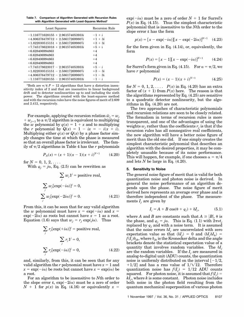
E. Generation of Several Families of Algorithms withRecursion Relations

Families of algorithms are now derived for phasesteps of 2py3, py2, py3, and py4 with a recursion ruleto increase the distortion insensitivity index by 1 togenerate successive member algorithms of each fam-ily. The first algorithm in each family will have qweights all equal to 1, where q is gotten from thephase step 2ppyq, where p and q are relatively primeintegers. Members of the py2, py3, and py4 familiesare insensitive to detector nonlinearities up to andincluding the quadratic, quartic, and sixth powers,respectively. We choose the recursion rules withpositive real coefficients that increase the number ofweights by the minimum each time. These recur-

sion rules are w# j 5 wj 1 wj11 1 wj12, w# j 5 wj 1 wj11,w# j 5 wj 1 wj11 1 wj12, and w# j 5 wj 1 wj12 for thefamilies with the phase steps of 2py3, py2, py3, andpy4, respectively. They are given in Tables 3, 4, 5,and 6, respectively. Their performance will be stud-ied in Section 7.

F. Connection to the Characteristic Polynomial Method

Any algorithm can be represented by a polynomial.Surrel9 represents an algorithm by the characteristicpolynomial

P~x! 5 (j50

P21

rjxj, (4.15)

where the rj are as defined in Eq. ~1.9!. We call thisthe r polynomial. An algorithm can also be repre-sented by the w polynomial

p~x! 5 (j50

P21

wjxj. (4.16)

Applying a recursion relation to the weights wj isequivalent to multiplying the r and w polynomials bypolynomial factors. In this work capital letters for rpolynomials and lower-case letters for w polynomialsare used. Applying the recursion relation,

w# j 5 (k50

N

akwj1k, (4.17)

is equivalent to multiplying the w polynomial by thefactor

q~x! 5 (k50

N

akxk, (4.18)

and is equivalent to multiplying the r polynomial bythe factor

Q~x! 5 (k50

N

ak exp~2ika!xk, (4.19)

where a is the phase step. Characteristic polynomi-als are only useful for a constant phase step.

Table 6. Family of Algorithms with Phase Step py4 Generated by #wj 5 wj 1 wj12a

P 5 8 1 1 1 1 1 1 1 1P 5 10 1 1 2 2 2 2 2 2 1 1P 5 12 1 1 3 3 4 4 4 4 3 3 1 1P 5 14 1 1 4 4 7 7 8 8 7 7 4 4 1 1P 5 16 1 1 5 5 11 11 15 15 15 15 11 11 5 5 1 1

aThis increases the distortion insensitivity index by 1 each time it is applied. The family is insensitive to detector nonlinearities withpowers as high as and including the sixth power.


For example, applying the recursion relation w# j 5 wj1 wj11 to a py2 algorithm is equivalent to multiplyingthe w polynomial by q~x! 5 1 1 x and to multiplyingthe r polynomial by Q~x! 5 1 2 ix 5 2 i~x 1 i!.Multiplying either q~x! or Q~x! by a phase factor sim-ply changes the time at which the phase is measuredso that an overall phase factor is irrelevant. The fam-ily of py2 algorithms in Table 4 has the r polynomials

PN~x! 5 ~x 1 1!~x 2 1!~x 1 i!N11 (4.20)

for N 5 0, 1, 2, . . . .With wj 5 ja, Eq. ~2.5! can be rewritten as

(j

wj1j 5 positive real,

(j

wj@exp~2ia!# j 5 0,

(j

wj@exp~22ia!# j 5 0. (4.21)

From this, it can be seen that for any valid algorithmthe w polynomial must have x 5 exp~2ia! and x 5exp~22ia! as roots but cannot have x 5 1 as a root.Equation ~1.6! says that wj 5 rj exp~ ja!. Thus

(j

rj@exp~1ia!# j 5 positive real,

(j

rj1j 5 0,

(j

rj@exp~2ia!# j 5 0, (4.22)

and, similarly, from this, it can be seen that for anyvalid algorithm the r polynomial must have x 5 1 andx 5 exp~2ia! be roots but cannot have x 5 exp~ia! bea root.

For an algorithm to be insensitive to Nth order tothe slope error ε, exp~22ia! must be a zero of orderN 1 1 for p~x! in Eq. ~4.16! or equivalently x 5

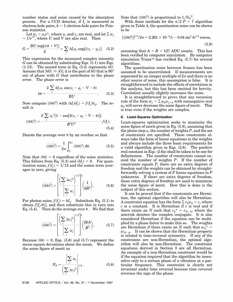
Table 7. Comparison of Algorithm Generated with Recursion Ruleswith Algorithm Generated with Least-Squares Methoda

Least Squares Recursion Rule

21.116771628155 1 2.961574053933i 21 1 i14.806376479712 1 2.586172699807i 11 1 3i11.822030515151 1 2.586172699807i 13 1 3i17.745178623018 1 2.961574053933i 15 1 i16.628406994863 1416.628406994863 1416.628406994863 1416.628406994863 1417.745178623017 2 2.961574053933i 15 2 i11.822030515151 2 2.586172699807i 13 2 3i14.806376479712 2 2.586172699807i 11 2 3i21.116771628155 2 2.961574053933i 21 2 i

aBoth are py4 P 5 12 algorithms that have a distortion insen-sitivity index of 2 and that are insensitive to linear backgrounddrift and to detector nonlinearities up to and including the sixthpower. The algorithms created with the least-squares methodand with the recursion rules have the noise figures of merit of 2.609and 2.412, respectively.

exp~2ia! must be a zero of order N 1 1 for Surrel’sP~x! in Eq. ~4.15!. Thus the simplest characteristicpolynomial that is insensitive to the Nth order to theslope error ε has the form

p~x! 5 @x 2 exp~2ia!#@x 2 exp~22ia!#N11 (4.23)

for the form given in Eq. ~4.14!, or, equivalently, theform

P~x! 5 @x 2 1#@x 2 exp~2ia!#N11 (4.24)

for Surrel’s form given in Eq. ~4.15!. For a 5 py2, wehave r polynomial

P~x! 5 ~x 2 1!~x 1 i!N11 (4.25)

for N 5 0, 1, 2, . . . . P~x! in Eq. ~4.20! has an extrafactor of ~x 1 1! from P~x! here. The reason is thatthe algorithms represented by Eq. ~4.25! are sensitiveto a quadratic detector nonlinearity, but the algo-rithms in Eq. ~4.20! are not.

The two approaches of characteristic polynomialsand recursion relations are seen to be closely related.The formalism in terms of recursion rules is moretransparent, and one of the advantages of using theweights wj rather than the coefficients rj is that if therecursion rules has all nonnegative real coefficients,the new algorithm will have a better noise figure ofmerit than the old one did. If one simply creates thesimplest characteristic polynomial that describes analgorithm with the desired properties, it may be com-pletely unusable because of its noise performance.This will happen, for example, if one chooses a 5 py4and lets N be large in Eq. ~4.20!.

5. Sensitivity to Noise

The general noise figure of merit that is valid for bothquantization noise and photon noise is derived. Ingeneral the noise performance of an algorithm de-pends upon the phase. The noise figure of meritderived here represents an average over phase and istherefore independent of the phase. The measure-ments Ij are given by

Ij 5 A 1 B cos~u 1 wj! 1 dIj, (5.1)

where A and B are constants such that A $ uBu, u isthe phase, and wj 5 ja. This is Eq. ~1.1! with 2pntjreplaced by wj and with a noise term. It is assumedthat the noise errors dIj are uncorrelated with zeroexpectation value so that ^dIj& 5 0 and ^dIjdIk& 5f ~Ij!djk, where djk is the Kronecker delta and the anglebrackets denote the statistical expectation value of aquantity that involves random variables. The dIjare the random variables. If the Ij are measured inanalog-to-digital unit ~ADU! counts, the quantizationnoise is uniformly distributed on the interval @21y2,11y2# and has a rms value of 1y=12. Thereforequantization noise has f ~Ij! 5 1y12 ADU countssquared. For photon noise, it is assumed that f ~Ij! 5kIj, where k is some constant. Photon noise includesboth noise in the photon field resulting from thequantum mechanical superposition of various photon


number states and noise caused by the absorptionprocess. For a CCD detector, if Ij is measured inelectron-hole pairs, k 5 1 electron-hole pairs for Pois-son statistics.

Let wj 5 ujevj, where uj and vj are real, and let ¥ wj

5 UeiV, where U and V are also real. Then

G 5BU exp@i~u 1 V!#

21 (

jdIjuj exp@i~nj 2 wj!#. (5.2)

This expression for the measured complex intensityG can be obtained by substituting Eqs. ~5.1! into Eqs.~1.13!. The second term in Eq. ~5.2! represents dG.Assume that udGu .. uGu; it is the part of dG that is 90°out of phase with G that contributes to the phaseerror. The phase error is

du 5

2 (j

dIjuj sin~nj 2 wj 2 V 2 u!

BU. (5.3)

Now compute ^~du!2& with ^dIidIj& 5 f ~Ij!dij. The re-sult is

^~du!2& 5

2 (j

uj2$1 2 cos@2~nj 2 wj 2 V 2 u!#%

B2U2 f ~Ij!.

(5.4)

Denote the average over u by an overbar so that

^~du!2& 51

2p *0

2p

^~du!2& du. (5.5)

Note that ^du& 5 0 regardless of the noise statistics.This follows from Eq. ~5.3! and ^dIj& 5 0. For quan-tization noise, f ~Ij! 5 1y12 and the cosine term aver-ages to zero, giving

^~du!2& 5 3S(juwj u2D1y2

U(j

wjU 42

S 16B2D . (5.6)

For photon noise, f ~Ij! 5 kIj. Substitute Eq. ~5.1! toobtain f @Ij~u!#, and then substitute this in turn intoEq. ~5.4!. Then do the average over u. We find that

^~du!2& 5 3S(juwj u2D1y2

U(j

wjU 42

S2kAB2 D . (5.7)

Because ^du& 5 0, Eqs. ~5.6! and ~5.7! represent themean-square deviations about the mean. We definethe noise figure of merit as

NF 5

U(j

wjUS(

juwj u2D1y2 . (5.8)


Note that ^~du!2& is proportional to 1yNF2.

With these methods for the py2 P 5 7 algorithmgiven in Table 4, the quantization noise can be shownto be

@^~du!2&#1y2y2p 5 2.261 3 1024~1 2 0.04 sin2 u!1y2 waves,

(5.9)

assuming that A 5 B 5 127 ADU counts. This hasbeen verified by computer simulation. By computersimulation Truax15 has verified Eq. ~5.7! for severalalgorithms.

The quantization noise between frames has beenassumed to be uncorrelated. If measurements areseparated by an integer multiple of 2p and there is noother source of noise, this assumption is false. It isstraightforward to include the effects of correlation inthe analysis, but this has been omitted for brevity.Correlation usually slightly increases the noise.

It is straightforward to prove that any recursionrule of the form w# j 5 ¥ akwj1k with nonnegative realak will never decrease the noise figure of merit. Thisis true even if the weights are complex.

6. Least-Squares Optimization

Least-squares optimization seeks to maximize thenoise figure of merit given in Eq. ~5.8!, assuming thatthe phase step a, the number of weights P, and the setof constraints are specified. These constraints al-ways take the form of linear equations in the weightsand always include the three basic requirements fora valid algorithm given in Eqs. ~2.6!. The positivereal constant in Eqs. ~2.6a! shall be taken to be one fordefiniteness. The number of constraints cannot ex-ceed the number of weights P. If the number ofconstraints equals P, there are no extra degrees offreedom and the weights can be obtained by straight-forwardly solving a system of P linear equations in Punknowns. If there are extra degrees of freedom,these extra degrees of freedom are used to maximizethe noise figure of merit. How this is done is thesubject of this section.

It can be proved that if the constraints are Hermi-tian, the optimal algorithm will also be Hermitian.A constraint equation has the form ¥ rkwk 5 c, wherec is a constant. It is Hermitian if c is real and ifthere exists an N such that rk* 5 rN2k, where theasterisk denotes the complex conjugate. It is alsoconsidered Hermitian if the equation can be multi-plied by a phase factor to make this so. The weightsare Hermitian if there exists an N such that wk* 5wN2k. It can be shown that the Hermitian propertyis related to time-reversal symmetry. If any of theconstraints are non-Hermitian, the optimal algo-rithm will also be non-Hermitian. The constraintequations derived in Section 3 are all Hermitian.An example of a non-Hermitian constraint would beif the equation required that the algorithm be insen-sitive only to a certain phase of a vibration at a par-ticular frequency. This constraint is clearly notinvariant under time reversal because time reversalreverses the sign of the phase.

The solution can be obtained after first finding anyvalid algorithm with the desired phase step a and thedesired number of weights P that satisfies the con-straints. Unless luck prevails, it will not have thebest possible noise performance. The optimized al-gorithm does not depend on the starting point. Theconstraints form an underdetermined system of lin-ear equations. The Eqs. ~2.6!, which any valid algo-rithm must satisfy, are included as three of theseconstraints. Equation ~2.6a! demands that the sumof the weights be positive real. Because multiplyingthe weights by a positive real constant does not rep-resent any real change in the algorithm, it can bedecided that the sum of the weights be 1. Later, ofcourse, the sum of the weights can be scaled to bewhatever is convenient. Finding one of the non-unique solutions for an underdetermined system oflinear equations is of course straightforward linearalgebra.

One constraint has the form

(k

wk 5 1, (6.1)

and the other constraints all have the form

(k

rk~a!wk 5 0, (6.2)

for a 5 1, 2, . . . , N, where N # P 2 1. The algo-rithm I start with is assumed to have weights wj thatsatisfy Eqs. ~6.1! and ~6.2!. Remember that the Eqs.~2.6b! and ~2.6c! give two of the sum rule constraintsin Eq. ~6.2!. The other sum rule constraints are ob-tained as discussed in Section 3. What they are de-pends upon what properties are desired in thealgorithm. I want to minimize ¥ uwku2 subject to theconstraints Eqs. ~6.1! and ~6.2!. Let z~b! be a set ofP 2 ~N 1 1! linearly independent vectors such that

(k

zk~b! wk 5 0, (6.3)

(k

rkzk~b! 5 0, (6.4)

where b 5 1, 2, . . . , P 2 ~N 1 1!. The vectors rk~a!

and wk span an ~N 1 1! dimensional space, while thevectors zk

~b! spans the P 2 ~N 1 1! dimensional space,which is orthogonal to the first space. The solutionwill be of the form

w# k 5 wk 1 (b

cbzk~b!, (6.5)

for some choice of the complex coefficients cb. Theconstraints of Eqs. ~6.3! and ~6.4! on the vectors zk

~b!

guarantee that the new weights w# k also satisfy Eqs.~6.1! and ~6.2!. The vectors zk

~b! are assumed to beorthogonal:

(k

zk~b!*zk

~b9! 5 Nbdbb9, (6.6)

where the asterisk indicates the complex conjugate.One can always find linear combinations of the zk

~b! tomake this so with Gram–Schmidt orthogonalization.

Now let us see how this optimization is carried out:

(k

uw# ku2 5 (k

uwku2 1 (b

(k

@cbw*kzk~b! 1 c*bwkzk

~b!*#

1 (bHcbc*b (

k@zk

~b!zk~b!*#J . (6.7)

The orthogonality relation Eq. ~6.6! has been used.Inspection of Eq. ~6.7! shows that optimization can bedone sequentially with respect to the coefficients cb ofthe vectors zk

~b!. This is because

(kFwk 1 (

b9Þb

cb9zk~b9!Gzk

~b!* 5 (k

wkzk~b!*. (6.8)

This should become clearer after reading the nextparagraph.

Let me therefore drop the subscript b and considerthe problem of minimizing ¥ uw# ku2 with respect to thecomplex coefficient c with w# k 5 wk 1 czk, where zk isone of the zk

~b!. Let c 5 a 1 ib, where a and b are real.Minimization can be accomplished by setting the par-tial derivatives of ¥ uw# ku2 with respect to a and b equalto zero. This is equivalent to regarding c and c* asindependent variables and setting the partial deriv-atives with respect to c and c* equal to zero. Doingso gives

(k

wk* zk 1 c* uzku2 5 0, (6.9a)

(k

wk zk* 1 c uzku2 5 0. (6.9b)

These two equations are just the complex conjugatesof each other, therefore just the second of the twoequations can be kept. Therefore

c 5

2 (k

wk zk*

(k

uzku2. (6.10)

Now it can be understood better what was assertedearlier about doing the minimization sequentially.Suppose I know what the coefficients cb are for all b9except b9 5 b. I then do the optimization with re-spect to this last unknown coefficient as describedabove:

cb 5

2 (kFwk 1 (

b9Þb

cb9zk~b9!Gzk

~b!*

(k

uzk~b!u2

. (6.11)


However, because of the orthogonality of zk~b!, Eq.

~6.11! can be simplified to

cb 5

2 (k

wkzk~b!*

(k

uzk~b!u2

(6.12)

Therefore no knowledge of the other coefficients cb isneeded. Equation ~6.12! is the main result of thissection.

As an example, choose a py4 phase step and 12frames. Require the algorithm to have a distortioninsensitivity index of 2, to be insensitive to linearbackground drift, and to be insensitive to detectornonlinearities as high as and including the sixthpower, which is the highest power that is possible fora py4 algorithm. One obtains the least-squares al-gorithm given in the first column of Table 7, whichhas the noise figure of merit 2.6096. The weightsare Hermitian. Now design this algorithm with re-cursion rules. Start with the P 5 8 algorithm withthe weights all 1. Apply the two-point complex re-cursion rule twice with Dj 5 1 for distortion insensi-tivity and then apply the two-point complex recursionrule once with Dj 5 2 for background drift. Oneobtains the algorithm in the second column whosenoise figure of merit is 2.4121.

7. Evaluation of Specific Algorithms

The kinds of phase errors that are produced by thevarious error sources are examined first. The mea-sured complex intensity G can always be written inthe form given by Eq. ~2.12!. Suppose that thedetector is linear so that only G2, G0, and G1 can benonzero, where G2 [ G21 and G1 [ G11. G1 mustalways be nonzero for a valid algorithm. First,suppose that the error source is such that G0 5 0but G2 Þ 0. This is true for PZT distortion errorsand signal drift. If the phase of G1 is not zero, itwill cause a phase error that is independent of u.Such an error is unimportant for phase-shifting in-terferometry. Consequently, it may be subtractedout. The part of the phase error that I am con-cerned with is thus given by

du 5 arg~G! 2 arg~G1! 2 u. (7.1)

Its extremes occur when G1 exp~1iu! and G2 exp~2iu!are 90° out of phase or when

u 512

argSG2

G1D 6

p

41 np. (7.2)

At these phases it has the extreme values

du 5 6tan21UG2

G1U . (7.3)

The exact equation for this type of phase error is

du 5 tan21S x sin y1 1 x cos yD ,


x 5 UG2

G1U y 5 argSG2

G1D 2 2u. (7.4)

The phase error du has period p in u and is zero wheny 5 np. Fringe print-through at twice the fringefrequency occurs when x is small.

Now suppose that the error source is such that G2

5 0 but G0 Þ 0. This is characteristic of backgrounddrift. The phase error is again given by Eq. ~7.1!.Its extremes occur when G1 exp~1iu! and G0 are 90°out of phase or when

u 5 argSG0

G1D 6

p

21 2np. (7.5)

The exact equation for this type of phase error is

du 5 tan21S x sin y1 1 x cos yD ,

x 5 UG0

G1U y 5 argSG0

G1D 2 u. (7.6)

The phase error du has period 2p in u and is zerowhen y 5 np. Fringe print-through at the fringefrequency occurs when x is small.

Finally, the effect of detector nonlinearity is con-sidered. A detector nonlinearity of power N cancause fringe print-through at all harmonics up to theN 1 1 harmonic in the first order. To prove this,rewrite Eq. ~3.9! as

G 5 H (m52N21

N21

Km~A, B, $an%!F(j

wj exp~imwj!G3 exp~imu!Jexp~iu!, (7.7)

and let arg~G! 5 u 1 du. When the coefficientsKm~A, B, $an%! are small, the phase error is givenapproximately by

du < (m52N21mÞ0

N21 UKm~A, B, $an%!

K0~A, B, $an%!U

3 sinHmu 1 argFKm~A, B, $an%!

K0~A, B, $an%!GJ . (7.8)

The constant K0~A, B, $an%! is always real.Look at the family of a 5 py2 algorithms whose

weights are given in Table 4. This family of py2algorithms was obtained through repeatedly apply-ing the recursion rule w# j 5 wj 1 wj11. These algo-rithms can be shown to be equivalent to the class Aalgorithms in Schmit and Creath.8 If this recursionrule is applied repeatedly to the three-frame py2 al-gorithm in Table 1, algorithms equivalent to theirclass B algorithms are obtained. The first algorithmin the Table 4 family is that py2 algorithm of fewestpoints that is insensitive to a quadratic detector non-linearity, which is the best possible for a py2 algo-rithm. py2 algorithms have a phase step 2ppyq,where the relatively prime integers p and q are p 5 1

and q 5 4. Thus the first algorithm in the familyhas q weights all equal to 1, as described in Subsec-tion 4.B. If only first-order distortion is present andthe weights are real symmetrical, G2~n0! is real be-cause the positive j terms are the complex conjugatesof the corresponding negative j terms in Eqs. ~3.1! ~ jwill vary from 2~P 2 1!y2 to 1~P 2 1!y2 in integersteps!. A phase error is caused when the G2~n0!e2iu

term has a component in quadrature to theG1~n0!e1iu term. For real G2~n0! and G1~n0!, thisphase error is given approximately:

du <G2~n0!

G1~n0!sin~2u!. (7.9)

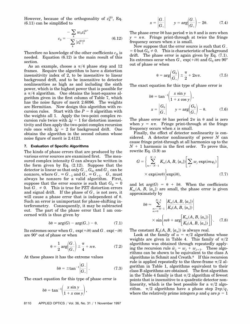
This is simple to obtain from Eq. ~7.4!. The phaseerror has its maximum magnitude when u 5 py4 1npy2, where n is any integer and is zero when u 5npy2. In Fig. 1, the a 5 py2 P 5 7, 9, 11, and 13optimally distortion-insensitive algorithms are com-pared. The phase error du is plotted versus the first-order distortion coefficient ε at u 5 45°, where du hasits greatest magnitude. For the small ε expected inphase-shift interferometry, the P 5 7 algorithmwould be good enough if higher-order distortionswere not a concern. The P 5 7 algorithm is insen-sitive up to and including the third order of first-orderdistortion and is insensitive to the first order of bothsecond- and third-order distortions but is sensitive tothe first order of fourth-order distortion. Even Palgorithms have not been presented in the plot be-cause, for even P, du is an odd function of ε ratherthan an even one so the plot could not have been log.Consider what happens if there is second-order distor-tion but no first-order distortion. Abbreviate g2 by gin this discussion. G1~n0, g! and G2~n0, g! are ob-tained from Eqs. ~3.1! by setting g3 5 g4 5 . . . 5 0 andreplacing g2 with g. Note that G1~n0, g! ceases to becompletely real, but that that part of du resulting fromarg@G1~n0, g!# is independent of u. For relative phaseerrors, only du 2 arg@G1~n0, g!# is important, and thisis what is examined here. Suppose that the algo-

Fig. 1. Absolute phase error du 5 arg@G~n0!# 2 u versus ε at u 545° for the P 5 7, 9, 11, and 13 a 5 py2 optimally distortion-insensitive algorithms whose weights are given in Table 4. Forsmall ε, du } εP23 sin 2u.

rithm is sensitive in rth order to second-order distor-tion but is insensitive in all lower orders. Because

G2~g! 512

B0 (j

wj exp@2pig~n0tj!2#exp~22iwj!, (7.10)

the dominant part of G2~g! is then

G2~g! <12

B0 (j

wj

@2pig~n0tj!2#r

r!exp~22iwj!. (7.11)

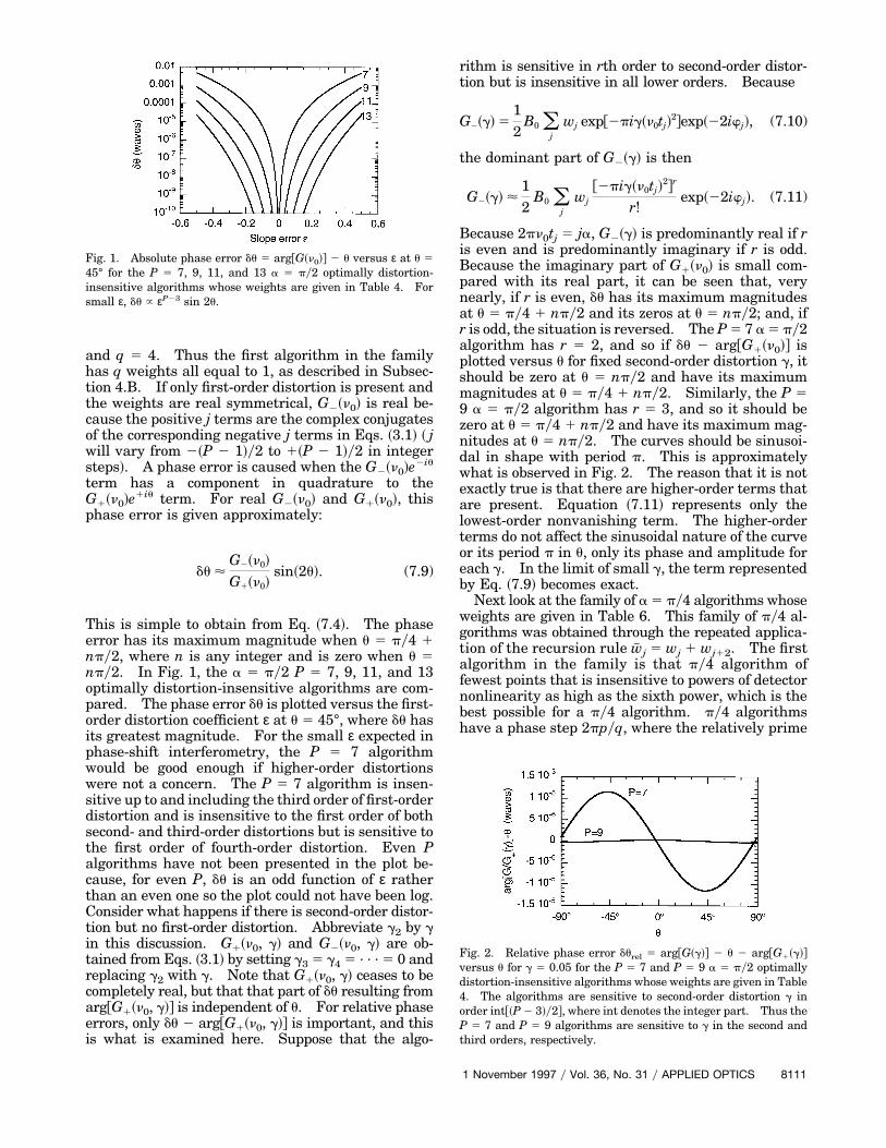
Because 2pn0tj 5 ja, G2~g! is predominantly real if ris even and is predominantly imaginary if r is odd.Because the imaginary part of G1~n0! is small com-pared with its real part, it can be seen that, verynearly, if r is even, du has its maximum magnitudesat u 5 py4 1 npy2 and its zeros at u 5 npy2; and, ifr is odd, the situation is reversed. The P 5 7 a 5 py2algorithm has r 5 2, and so if du 2 arg@G1~n0!# isplotted versus u for fixed second-order distortion g, itshould be zero at u 5 npy2 and have its maximummagnitudes at u 5 py4 1 npy2. Similarly, the P 59 a 5 py2 algorithm has r 5 3, and so it should bezero at u 5 py4 1 npy2 and have its maximum mag-nitudes at u 5 npy2. The curves should be sinusoi-dal in shape with period p. This is approximatelywhat is observed in Fig. 2. The reason that it is notexactly true is that there are higher-order terms thatare present. Equation ~7.11! represents only thelowest-order nonvanishing term. The higher-orderterms do not affect the sinusoidal nature of the curveor its period p in u, only its phase and amplitude foreach g. In the limit of small g, the term representedby Eq. ~7.9! becomes exact.

Next look at the family of a 5 py4 algorithms whoseweights are given in Table 6. This family of py4 al-gorithms was obtained through the repeated applica-tion of the recursion rule w# j 5 wj 1 wj12. The firstalgorithm in the family is that py4 algorithm offewest points that is insensitive to powers of detectornonlinearity as high as the sixth power, which is thebest possible for a py4 algorithm. py4 algorithmshave a phase step 2ppyq, where the relatively prime

Fig. 2. Relative phase error durel 5 arg@G~g!# 2 u 2 arg@G1~g!#versus u for g 5 0.05 for the P 5 7 and P 5 9 a 5 py2 optimallydistortion-insensitive algorithms whose weights are given in Table4. The algorithms are sensitive to second-order distortion g inorder int@~P 2 3!y2#, where int denotes the integer part. Thus theP 5 7 and P 5 9 algorithms are sensitive to g in the second andthird orders, respectively.


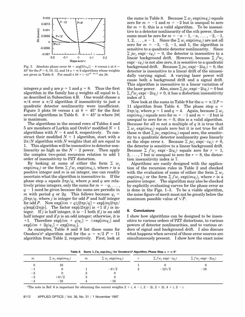
integers p and q are p 5 1 and q 5 8. Thus the firstalgorithm in the family has q weights all equal to 1,as described in Subsection 4.B. One would choose apy4 over a py2 algorithm if insensitivity to just aquadratic detector nonlinearity were insufficient.Figure 3 plots du versus ε at u 5 45° for the firstseveral algorithms in Table 6. u 5 45° is where uduuis maximum.

The algorithms in the second rows of Tables 4 and5 are members of Larkin and Oreb’s4 modified N 1 1algorithms with N 5 4 and 8, respectively. To con-struct their modified N 1 1 algorithm, start with a2pyN algorithm with N weights that all are equal to1. This algorithm will be insensitive to detector non-linearity as high as the N 2 2 power. Then applythe complex two-point recursion relation to add 1order of insensitivity to PZT distortion.

By looking at sums of either the form ¥ wjexp~imwj! or the form ¥ jrwj exp~imwj!, where r is apositive integer and m is an integer, one can readilyascertain what the algorithm is insensitive to. If thephase step a equals 2ppyq, where p and q are rela-tively prime integers, only the sums for m 5 2q, . . . ,q 2 1 need be given because the sums are periodic inm with period q or 2q. This follows because wj 5j2ppyq, where j is integer for odd P and half integerfor odd P. Now exp@i~m 1 q! j2ppyq# 5 exp@imj2ppyq#exp@i2pjp#. The factor exp@i2pjp# is 11 if j is in-teger. If j is half integer, it is 21 both if j is an oddhalf integer and if p is an odd integer; otherwise, it is11. Therefore exp@i~m 1 q!wj# 5 6exp@imwj# andexp@i~m 1 2q!wj# 5 exp@imwj#.

As examples, Table 8 and 9 list these sums forOnodera’s6 algorithm and for the a 5 py2 P 5 11algorithm from Table 2, respectively. First, look at

Fig. 3. Absolute phase error du 5 arg@G~n0!# 2 u versus ε at u 545° for the P 5 8, 10, 12, and 14 a 5 py4 algorithms whose weightsare given in Table 6. For small ε du } ~2ε!~P26!y2 sin 2u.

the sums in Table 8. Because ¥ wj exp~imwj! equalszero for m 5 21 and m 5 22 but is unequal to zerofor m 5 0, this is a valid algorithm. To be insensi-tive to a detector nonlinearity of the nth power, thesesums must be zero for m 5 2n 2 1, 2n, . . . , 22, 21,1, 2, . . . , n 2 1. Since the ¥ wj exp~imwj! are not allzero for m 5 23, 22, 21, and 1, the algorithm issensitive to a quadratic detector nonlinearity. Since¥ jwj exp~2iwj! 5 0, the detector is insensitive to alinear background drift. However, because ¥ j2wjexp~2iwj! is not also zero, it is sensitive to a quadraticbackground drift. Because ¥ jwj exp~22iwj! 5 0, thedetector is insensitive to a linear drift of the sinusoi-dally varying signal. A varying laser power willcause both a background drift and a signal drift.This algorithm is insensitive to a linear variation ofthe laser power. Also, since ¥ jwj exp~22iwj! 5 0 but¥ j2wj exp~22iwj! Þ 0, it has a distortion insensitivityindex of 1.

Now look at the sums in Table 9 for the a 5 py2 P 511 algorithm from Table 4. The phase step a 52ppyq, where p 5 1 and q 5 4. Again, because ¥ wjexp~imwj! equals zero for m 5 21 and m 5 22 but isunequal to zero for m 5 0, this is a valid algorithm.Because for all m not a multiple of q it is true that¥ wj exp~imwj! equals zero but it is not true for allthese m that ¥ jwj exp~imwj! equal zero, the sensitiv-ity to a quadratic detector nonlinearity goes linearlyas the slope error ε. Because ¥ jwj exp~2iwj! Þ 0,the detector is sensitive to a linear background drift.Because ¥ jrwj exp~22iwj! equals zero for r 5 1,2, . . . , 7 but is unequal to zero for r 5 8, the distor-tion insensitivity index is 7.

Algorithms are easily designed with the applica-tion of the recursion rules in Table 2 and checkedwith the evaluation of sums of either the form ¥ wjexp~imwj! or the form ¥ jrwj exp~imwj!, where r is apositive integer. The algorithm may also be checkedby explicitly evaluating curves for the phase error asis done in the Figs. 1–3. To be a viable algorithm,the noise figure of merit must not be greatly below themaximum possible value of =P.

8. Conclusions

I show how algorithms can be designed to be insen-sitive to various orders of PZT distortions, to variouspowers of detector nonlinearities, and to various or-ders of signal and background drift. I also discusswhat happens when several of these error sources aresimultaneously present. I show how the exact noise

Table 8. Sums S jrwj exp~imwj! for Onodera’s6 Algorithm; Phase Step a 5 py2a

m ¥ wj exp~imwj! m ¥ wj exp~imwj! r ¥ jrwj exp~2iwj! ¥ jrwj exp~22iwj!

0 16 1 0 021 0 1 28=2 2 212=2 21622 0 2 023 18=2 3 024 216 4 216

aThe note in Ref. 6 is important for obtaining the correct weights 2 1 i, 4 2 i, 2 2 2i, 2 1 2i, 4 1 i, 2 2 i.


Table 9. Sums S jrwj exp ~imwj! for the P 5 11 a 5 py2 Algorithm from Table 4a

m ¥ wj exp~imwj! m ¥ wj exp~imwj! m¥ jwj

exp~imwj! m¥ jwj

exp~imwj! r ¥ jrwj exp~2iwj! ¥ jrwj exp~22iwj!

0 512 0 0 1 232i 021 0 1 0 21 232i 1 32i 2 2256 022 0 2 0 22 0 2 0 3 1120i 023 0 3 0 23 32i 3 32i 4 2048 024 512 4 512 24 0 4 0 5 7648i 0

6 57344 07 229600i 08 1015808 280640

aWeight w 5 1 8 29 64 98 112 98 64 29 8 1.

statistics may be computed for a specific algorithmand derive a general noise figure of merit valid forany algorithm. Algorithms can be designed with theapplication of recursion rules to an existing algo-rithm. The minimal algorithms are the three-pointalgorithms given in Table 1. The minimal algorithmfor a phase step a 5 2ppyq that is insensitive todetector nonlinearities as high as the q 2 2 power hasq weights that are all equal to 1. The basic opera-tion in the recursion rules is the linear transforma-tion w# j 5 ¥ a~k!wj1k. If the sum is from k 5 0 to k 5n, an2k 5 ak*, where the asterisk denotes complexconjugation. This ensures that the new algorithmwill have Hermitian weights if the original algorithmdid. In addition, if the coefficients a~k! are all non-negative real, the new algorithm will have all non-negative real weights if the original one did. If theweights when summed nearly cancel, the noise figureof merit will be small and the algorithm’s perfor-mance in the presence of noise will be abysmal. Therecursion rules must be applied judicially to ensurethis does not happen.

I have come up with families of algorithms for thephase steps of 2py3, py2, py3, and py4 for whichsuccessive members are generated by the recursionrules w# j 5 wj 1 wj11 1 wj12, w# j 5 wj 1 wj11, w# j 5 wj1 wj11 1 wj12, and w# j 5 wj 1 wj12, respectively.These recursion rules increase the distortion insen-sitivity index by 1. The first algorithm in each fam-ily has q points, where q is obtained from the phasestep 2ppyq. Here p and q are relatively prime inte-gers. The py2, py3, and py4 families of algorithmsare insensitive to powers of detector nonlinearities ashigh as the quadratic, quartic, and sixth powers, re-spectively. The 2py3, py2, py3, and py4 families ofalgorithms are presented in Tables 3, 4, 5, and 6,respectively.

I also derive a noise figure of merit that is valid forany algorithm and present a least-squares method forobtaining that unique algorithm that maximizes thenoise figure of merit and satisfies a set of constraintequations upon the weights that give the algorithm acertain set of desired properties.

Appendix A: Three-Point Algorithm for Any Phase Step

Equations ~2.5! give the three conditions that anyalgorithm must satisfy. With three weights, one has

three equations in three unknowns. Let the threeweights be w21, w0, and w11. I replace the firstcondition by w0 5 1 and suppose that this guaranteesthat the sum of the weights is nonzero. This is ver-ified after a solution is obtained. Letting x 5 e2ia,the following matrix equation is obtained:

F 0x21

x22

111

0x1

x2GFw21

w0

w11

G 5 F100G . (A1)

This is a matrix equation of the form ¥ Aijuj 5 Bi,where the sum is over j. The solution is straightfor-ward:

Fw21

w0

w1

G 5 F 2x2y~1 1 x!1

~2x2y~1 1 x!!*G . (A2)

Here the asterisk denotes the complex conjugate.x21 5 x* is used. The weights in Eq. ~A2! are Her-mitian. This is expected: The matrix Aij is un-changed by reversing the order of its columns andtaking the complex conjugate ~note that x21 5 x*!.Any matrix equation ¥ Aijuj 5 Bi is unchanged byreordering the columns of Aij and the rows of uj in thesame fashion. Let us reverse the order of the col-umns in Aij and reverse the order of the rows in uj andthen take the complex conjugate. What results anequation the same as Eq. ~A1! except that w21, w0,and w11 are replaced by w11*, w0*, and w21*, respec-tively. Because the solution is unique, w0 must bereal and w21 and w11 must be complex conjugates.

The weights will sum to zero if the real part of2x2y~1 1 x! is 21y2. This occurs if cos~3ay2! 5cos~ay2!. Now cos~3ay2! 5 4 cos3~ay2! 2 3 cos~ay2!.Therefore the weights will sum to zero if cos3~ay2! 5cos~ay2!. This can occur only if cos~ay2! 5 0 or 61or, equivalently, if a is a multiple of p. There are novalid phase-shifting interferometry algorithms whenthe phase step is a multiple of p.

The three-point algorithms for the phase steps a5 2py3, py2, py3, and py4 are listed in Table 1.The weights w21, w0, and w11 are given in thesecond, third, and fourth columns, respectively, andthe arctangent formulas for the phase u are given inthe last column. The general arctangent form of


the three-point algorithm with phase step a is u 5tan21 $tan~ay2!@I21 2 I1#y@2I0 2 I1 2 I21#%. Thenext to last column in Table 1 lists the noise figureof merit u¥ wjuy~¥ uwju

2!1y2. This can be evaluatedmost directly with the relations u¥ wju 5 2~1 2 cos a!and ¥ uwju

2 5 1 1 1y~1 1 cos a!. For a 5 2py3, py2,py3, and py4, the noise figures of merit are =3, 1,=~3y5!, and ~2 2 =2!y~3 2 =2!1y2, respectively.For small a, the noise figure of merit approaches=~2y3!a2. The three-point a 5 py4 algorithm istoo susceptible to noise to make it a practical algo-rithm. The a 5 2py3 algorithm has the best pos-sible noise figure of merit for a three-pointalgorithm because all its weights are 1. All three-point algorithms are sensitive to PZT distortions,detector nonlinearities, and laser power drift.

One may transform any formula of the form u 5tan21~¥ bjIjy¥ ajIj! to a formula of the form u 5 u0 1tan21~¥ b# jIjy¥ a# jIj! for any arbitrary u0. For instance,u 5 tan21 @~I0 2 I1!y~I0 2 I21!# 2 py4 is an alter-native form for the py2 P 5 3 algorithm.

Appendix B: Recursion Relations to EliminateSensitivity to a Particular Frequency of Vibration

Suppose an existing algorithm has the desired prop-erties except for insensitivity to a small amplitudevibration at the frequency nvib and suppose that fromthis existing algorithm I want to create a new algo-rithm that retains all the desired properties of theoriginal algorithm except that it is insensitive to asmall amplitude vibration at frequency nvib. I firstfind the recursion relations of the form

w# j 5 exp~2ib!wj 1 exp~ib!wj1Dj, (B1)

which make G2~n0! and G1~n0! be zero at n0 5 n 6nvib. For relative insensitivity to a frequency of vi-bration, all that is necessary is that G2~n0! be zero atn0 5 n 6 nvib. Relative insensitivity is all that isimportant for phase-shift interferometry. With themethods already familiar from Section 4, it can befound that

b 5

p 2 Sn0

n1 1DaDj

2f G# 2~n0! 5 0,

b 5

Sn0

n2 1DaDj 2 p

2f G# 1~n0! 5 0. (B2)

Here a is the phase step, Dj is a positive integer, and

G# 5 (j

w# jIj exp~2iwj!. (B3)

To make the algorithm relatively insensitive to a vi-bration of a particular frequency, it is necessary thatG2~n0! be zero at n0 5 n 6 nvib. This means that forDj 5 1, two new weights are required for each fre-quency to which the algorithm should be made insen-sitive.


Also considered is a recursion rule of the type

w# j 5 a2wj2Dj 1 a0wj 1 a1wj1Dj (B4)

with a1 5 a2 and a2, a0, and a1 all real. It isnecessary to find how to make

(j

w# j exp~ijxa! 5 0 (B5)

where a is the phase step and x is a number. Tomake G# 1~n0! vanish, I set x 5 21 1 n0yn, and to makeG# 2~n0! vanish, I set x 5 21 2 n0yn. For Eq. ~B5! tobe satisfied, I must have

a0 1 a1 cos~xaDj! 5 0. (B6)

One must always examine the noise performance ofan algorithm after recursion relation is applied tomake sure that it is acceptable. If the sums of thecoefficients of the recursion relation sum to nearlyzero, it is likely that the resulting algorithm will havean exceedingly poor noise performance. The sum ofthe recursion coefficients is exp~ib! 1 exp~2ib! in Eq.~B1! and a2 1 a0 1 a1 in Eq. ~B4!.

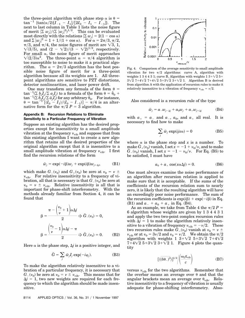
As an example, we take from Table 4 the py2 P 56 algorithm whose weights are given by 1 3 4 4 3 1and apply the two two-point complex recursion ruleswith Dj 5 1 to make the algorithm relatively insen-sitive to a vibration of frequency nvib 5 2ny2. Thesetwo recursion rules make G# 2~n0! vanish at n0 5 n 6nvib or at n0 5 3ny2 and n0 5 ny2. We obtain the py2algorithm with weights 1 31=2 513=2 714=2714=2 513=2 31=2 1. Figure 4 plots the quan-tity

@^~du2!2&#1y2YSvLεvib

c D (B7)

versus nvib for the two algorithms. Remember thatthe overbar means an average over u and that theangular brackets mean an average over uvib. Rela-tive insensitivity to a frequency of vibration is usuallyadequate for phase-shifting interferometry. Abso-

Fig. 4. Comparison of the average sensitivity to small amplitudevibration for two py2 algorithms: curve A, algorithm withweights 1 3 4 4 3 1; curve B, Algorithm with weights 1 31=2 513=2 714=2 714=2 513=2 31=2 1. Algorithm B is derivedfrom algorithm A with the application of recursion rules to make itrelatively insensitive to a vibration of frequency nvib 5 ny2.

lute insensitivity would be required if, for example,different parts of a test optic vibrated differently.

The author thanks Gary Sommargren, BruceTruax, Gene Campbell, and the referees for their crit-icism and suggestions. This work was performedunder the auspices of the U.S. Department of Energyby Lawrence Livermore National Laboratory undercontract W-7405-Eng-48.

The author’s e-mail address is [email protected].

References and Notes1. K. Creath, “Phase measurement interferometry techniques,”

in Progress in Optics, E. Wolf, ed. ~Elsevier, New York, 1988!,Vol. 26, Chap. 5, pp. 349–383.

2. J. C. Wyant, “Interferometric optical metrology: basic princi-ples and new systems,” Laser Focus 18, 65–71 ~May 1982!.

3. P. de Groot, “Derivation of algorithms for phase-shifting inter-ferometry using the concept of a data-sampling window,” Appl. Opt.34, 4723–4730 ~1995!. His values of ε and g for py2 algorithmsare, respectively, 2py2 and py16 times the values in this paper.

4. K. G. Larkin and B. F. Oreb, “Design and assessment of sym-metrical phase-shifting algorithms,” J. Opt. Soc. Am. A 9,1740–1748 ~1992!.

5. K. Freischlad and C. L. Koliopoulos, “Fourier description ofdigital phase-shifting interferometry,” J. Opt. Soc. Am. A 7,542–551 ~1990!.

6. R. Onodera and Y. Ishii, “Phase extraction analysis of laser-

diode phase-shifting interferometry that is insensitive tochanges in laser power,” J. Opt. Soc. Am. A 13, 139–146 ~1996!.Their formula for the phase has the form u 5 tan21 ~¥ bjIjy¥ aiIi!, and their phase step is really 2py2. For 1py2 phasestep, let bj 3 2bj.

7. C. J. Morgan, “Least squares estimation in phase-measurement interferometry,” Opt. Lett. 7, 368–370 ~1982!.

8. J. Schmit and K. Creath, “Extended averaging technique forderivation of error-compensating algorithms in phase-shiftinginterferometry,” Appl. Opt. 34, 3610–3619 ~1995!.

9. Y. Surrel, “Design of algorithms for phase measurements bythe use of phase-shifting,” Appl. Opt. 35, 51–60 ~1996!.

10. J. Schwider, R. Burow, K. E. Elssner, J. Grzanna, R. Spola-czyk, and K. Merkel, “Digitial wave-front measuring inter-ferometry: some systematic error sources,” Appl. Opt. 22,3421–3432 ~1983!.

11. P. Hariharan, B. F. Oreb, and T. Eiju, “Digital phase-shiftinginterferometry: a simple error-compensating phase calcula-tion algorithm,” Appl. Opt. 26, 2504–2507 ~1987!.

12. P. de Groot, “Vibration in phase-shifting interferometry,” J.Opt. Soc. Am. A 12, 354–365 ~1995!.

13. J. E. Grievenkamp, “Generalized data reduction for hetero-dyne interferometry,” Opt. Eng. 23, 350–352 ~1984!.

14. P. Wizinowich, “Phase shifting interferometry in the presenceof vibration: a new algorithm and system,” Appl. Opt. 29,3271–3279 ~1990!.

15. B. Truax, Truax Associates, 189 Olson Drive, Southington,Conn. 06489 ~personal communication, 1997!.


Documents

General methods for generating phase-shifting interferometry algorithms