Embed Size (px)
Citation preview

General Linear Model (Chapter 4): Part 3
• Examining moderators (i.e interactions)
• Examining linearity and testing for trend with categorical predictors
• Assessing the model: heteroscedasticity, outliers, multicollinearity

Implication of Main Effects model
KEY ASSUMPTION: Every variable has the same effect on the outcome within every other category of every other variable, e.g. the effect that sports has on GPA is the same for both cohorts. Or visa versa, the effect that cohort has on GPA is the same whether the kid plays sports or not.
2.7
2.7
52
.82
.85
2.9
2.9
5G
PA
0 .2 .4 .6 .8 1Sports team
junior high
high school

How to obtain the Estimates on previous plot proc glm data = gpa_c;
class race;
model gpa = mvpa_hours dgender numcohort ses_s c_numsport race /solution;
estimate "no sport junior high" c_numsport 0 numcohort 0
intercept 1 dgender .5 ses_s 3 race .52 .16 .06 .20 .03 .03 mvpa_hours 6.6;
estimate "sports junior high" c_numsport 1 numcohort 0
intercept 1 dgender .5 ses_s 3 race .52 .16 .06 .20 .03 .03 mvpa_hours 6.6;
estimate "no sports high school" c_numsport 0 numcohort 1
intercept 1 dgender .5 ses_s 3 race .52 .16 .06 .20 .03 .03 mvpa_hours 6.6;
estimate "sports high school" c_numsport 1 numcohort 1
intercept 1 dgender .5 ses_s 3 race .52 .16 .06 .20 .03 .03 mvpa_hours 6.6;
run;
Standard
Parameter Estimate Error t Value Pr > |t|
no sport junior high 2.83434336 0.06297755 45.01 <.0001
sports junior high 2.96297904 0.05271679 56.21 <.0001
no sports high school 2.69010261 0.04737569 56.78 <.0001
sports high school 2.81873829 0.03963993 71.11 <.0001
Standard
Parameter Estimate Error t Value Pr > |t|
Intercept 1.973181868 B 0.16151324 12.22 <.0001
mvpa_hours 0.006178674 0.00603294 1.02 0.3060
dgender 0.240793587 0.05392039 4.47 <.0001
numcohort -0.144240750 0.05887527 -2.45 0.0145
ses_s 0.142327935 0.02255155 6.31 <.0001
c_numsport 0.128635679 0.05905180 2.18 0.0296
race 1 0.354133454 B 0.14246109 2.49 0.0131
race 2 0.084365698 B 0.14952955 0.56 0.5727
race 3 -0.178735243 B 0.17053048 -1.05 0.2948
race 4 0.442756541 B 0.14874401 2.98 0.0030
race 6 -0.082448488 B 0.20020479 -0.41 0.6806
race 7 0.000000000 B . . .
* In Stata, use
-lincom- command

Implication of Main Effects model
Model assumes that slope of MVPA on GPA is the same within every race
category. Or visa versa, the effect that race has on GPA is the same for every
level of MVPA.

Interactions or moderators or effect modifiers
Interactions or moderators or effect modifiers
• What if we want to examine whether sports have a differential effect on GPA
in junior high as compared to high school.
• What if we are interested to see if MVPA relates to GPA differently across the
races?
These questions can be addressed by including an interaction term (a product
term) as another predictor into the linear model.
Notice that in both questions above, we have identified the “predictor of
interest” and the modifier of interest in the way the question is asked. What is
the predictor of interest and what is the modifier?
Despite the question of interest, when we examine an interaction, both
variables in the interaction are moderating each other.

Include interaction term - Sports*cohort . reg gpa mvpa_hours i.c_numsport##i.numcohort gender ses_s i.race
Source | SS df MS Number of obs = 1000
-------------+------------------------------ F( 11, 988) = 12.74
Model | 97.2019287 11 8.83653897 Prob > F = 0.0000
Residual | 685.541821 988 .69386824 R-squared = 0.1242
-------------+------------------------------ Adj R-squared = 0.1144
Total | 782.74375 999 .783527277 Root MSE = .83299
--------------------------------------------------------------------------------------
gpa | Coef. Std. Err. t P>|t| [95% Conf. Interval]
---------------------+----------------------------------------------------------------
mvpa_hours | .0062441 .0060288 1.04 0.301 -.0055867 .0180748
1.c_numsport | -.0040722 .1039472 -0.04 0.969 -.2080549 .1999104
1.numcohort | -.2639563 .0970597 -2.72 0.007 -.454423 -.0734895
|
c_numsport#numcohort |
1 1 | .1880543 .1212626 1.55 0.121 -.0499074 .4260161
|
gender | .2435666 .0539118 4.52 0.000 .1377719 .3493614
ses_s | .1420196 .0225364 6.30 0.000 .0977948 .1862443
|
race |
2 | -.2583253 .0771352 -3.35 0.001 -.4096929 -.1069576
3 | -.5272124 .1134827 -4.65 0.000 -.7499071 -.3045176
4 | .0921568 .0763627 1.21 0.228 -.057695 .2420086
6 | -.4220401 .153544 -2.75 0.006 -.7233499 -.1207302
7 | -.3373028 .1427731 -2.36 0.018 -.6174762 -.0571295
|
_cons | 2.40941 .1241965 19.40 0.000 2.165691 2.65313
--------------------------------------------------------------------------------------
Why 11 d.f. for whole model? Notice the interaction has 1 d.f. because (2-1)*(2-1). Notice the interaction is not significant with p-value = .121.

Interpretation of interaction term - Sports*cohort
Ignoring the non-significant p-value, we can interpret the interaction term
between sports and cohort as:
The effect that sports has on GPA for kids in High school is 0.188 points
higher than the effect sports has in Jr. High. This also can be turned around the
other way remember the moderate each other), the difference between High
school and Jr high GPA is 0.188 points higher for those in sports compared to
those who aren’t in sports.
Note: in the original study, a significant sport*cohort interaction was
identified. Here we are only using a proportion of the original data (<25%), so
the test is under-powered. In general, test for interaction requires larger sample
size than that for main effects.
SAS code: proc glm data = gpa_c;
class race;
model gpa = mvpa_hours dgender numcohort ses_s c_numsport
race c_numsport*numcohort/solution;
run;

Interaction
Sports
(α)
Junior/high
(β)
Interaction
(γ)
Change in
GPA
1 1 1 α + β + γ
1 0 0 α
0 1 0 β
0 0 0
Interpretation of Interaction term: The effect that sports has on
GPA for kids in High school (α + β + γ – β = α + γ ) is 0.188 points
higher than the effect sports has in Jr. High (α).
Alternatively, the difference between High school and Jr High
GPA is 0.188 points higher for those in sports (α + β + γ – α = β +
γ ) compared to those who aren’t in sports (β).
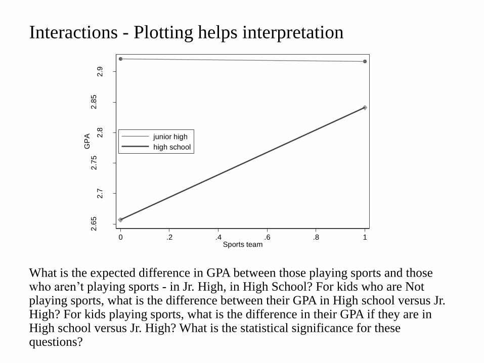
Interactions - Plotting helps interpretation
What is the expected difference in GPA between those playing sports and those who aren’t playing sports - in Jr. High, in High School? For kids who are Not playing sports, what is the difference between their GPA in High school versus Jr. High? For kids playing sports, what is the difference in their GPA if they are in High school versus Jr. High? What is the statistical significance for these questions?
2.6
52
.72
.75
2.8
2.8
52
.9
GP
A
0 .2 .4 .6 .8 1Sports team
junior high
high school
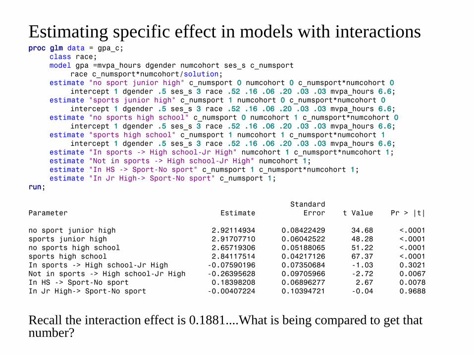
Estimating specific effect in models with interactions proc glm data = gpa_c; class race; model gpa =mvpa_hours dgender numcohort ses_s c_numsport race c_numsport*numcohort/solution; estimate "no sport junior high" c_numsport 0 numcohort 0 c_numsport*numcohort 0 intercept 1 dgender .5 ses_s 3 race .52 .16 .06 .20 .03 .03 mvpa_hours 6.6; estimate "sports junior high" c_numsport 1 numcohort 0 c_numsport*numcohort 0 intercept 1 dgender .5 ses_s 3 race .52 .16 .06 .20 .03 .03 mvpa_hours 6.6; estimate "no sports high school" c_numsport 0 numcohort 1 c_numsport*numcohort 0 intercept 1 dgender .5 ses_s 3 race .52 .16 .06 .20 .03 .03 mvpa_hours 6.6; estimate "sports high school" c_numsport 1 numcohort 1 c_numsport*numcohort 1 intercept 1 dgender .5 ses_s 3 race .52 .16 .06 .20 .03 .03 mvpa_hours 6.6; estimate "In sports -> High school-Jr High" numcohort 1 c_numsport*numcohort 1; estimate "Not in sports -> High school-Jr High" numcohort 1; estimate "In HS -> Sport-No sport" c_numsport 1 c_numsport*numcohort 1; estimate "In Jr High-> Sport-No sport" c_numsport 1; run; Standard Parameter Estimate Error t Value Pr > |t| no sport junior high 2.92114934 0.08422429 34.68 <.0001 sports junior high 2.91707710 0.06042522 48.28 <.0001 no sports high school 2.65719306 0.05188065 51.22 <.0001 sports high school 2.84117514 0.04217126 67.37 <.0001 In sports -> High school-Jr High -0.07590196 0.07350684 -1.03 0.3021 Not in sports -> High school-Jr High -0.26395628 0.09705966 -2.72 0.0067 In HS -> Sport-No sport 0.18398208 0.06896277 2.67 0.0078 In Jr High-> Sport-No sport -0.00407224 0.10394721 -0.04 0.9688
Recall the interaction effect is 0.1881....What is being compared to get that number?

Interacting a continuous and a categorical variable proc glm data = gpa_c; class race; model gpa = mvpa_hours dgender numcohort ses_s c_numsport race mvpa_hours*race/solution; run;
Source DF Type III SS Mean Square F Value Pr > F mvpa_hours 1 0.00038359 0.00038359 0.00 0.9813 dgender 1 13.73139451 13.73139451 19.71 <.0001 numcohort 1 4.08914812 4.08914812 5.87 0.0156 ses_s 1 27.73392947 27.73392947 39.81 <.0001 c_numsport 1 3.09573791 3.09573791 4.44 0.0353 race 5 12.22741867 2.44548373 3.51 0.0038 mvpa_hours*race 5 1.73059819 0.34611964 0.50 0.7788 Standard Parameter Estimate Error t Value Pr > |t| Intercept 1.956900672 B 0.24510684 7.98 <.0001 mvpa_hours 0.008832261 B 0.03015503 0.29 0.7697 dgender 0.240107747 0.05408149 4.44 <.0001 numcohort -0.143077735 0.05905484 -2.42 0.0156 ses_s 0.142828347 0.02263646 6.31 <.0001 c_numsport 0.124941860 0.05926874 2.11 0.0353 race 1 0.347018738 B 0.24597593 1.41 0.1586 race 2 0.100044366 B 0.25437714 0.39 0.6942 race 3 -0.191711178 B 0.28710276 -0.67 0.5045 race 4 0.473732170 B 0.25392450 1.87 0.0624 race 6 0.280254490 B 0.36120364 0.78 0.4380 race 7 0.000000000 B . . . mvpa_hours*race 1 0.000443924 B 0.03105651 0.01 0.9886 mvpa_hours*race 2 -0.002468278 B 0.03304383 -0.07 0.9405 mvpa_hours*race 3 0.002818875 B 0.03824333 0.07 0.9413 mvpa_hours*race 4 -0.005313166 B 0.03324176 -0.16 0.8730 mvpa_hours*race 6 -0.047206110 B 0.04239700 -1.11 0.2658 mvpa_hours*race 7 0.000000000 B . . .
Interacting a continuous and a categorical variable
What would the Total Model d.f. be?
Why 5 d.f. for the interaction?
What does the interaction term being non-significant imply?
How do we interpret the estimates for the interactions?
Note: Although the interaction terms are non-significant, the p-values for
RACE main effects become less significant compared to the main effects only
model. Why?

Plot interactions
There is not enough statistical evidence to say that these lines are NOT
PARALLEL. P-value for interactions = 0.7788
mvpa_hours*race effect plot
mvpa_hours
gpa
2
2.5
3
0 5 10 15
: race 1 : race 2
0 5 10 15
: race 3
: race 4
0 5 10 15
: race 6
2
2.5
3
: race 7
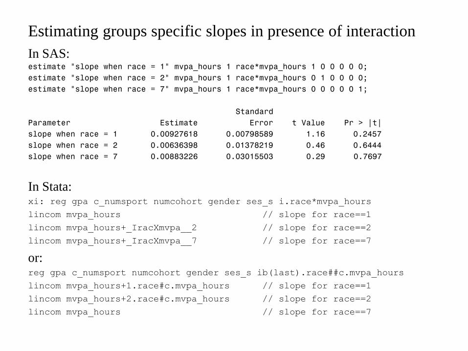
Estimating groups specific slopes in presence of interaction
In SAS: estimate "slope when race = 1" mvpa_hours 1 race*mvpa_hours 1 0 0 0 0 0;
estimate "slope when race = 2" mvpa_hours 1 race*mvpa_hours 0 1 0 0 0 0;
estimate "slope when race = 7" mvpa_hours 1 race*mvpa_hours 0 0 0 0 0 1;
Standard
Parameter Estimate Error t Value Pr > |t|
slope when race = 1 0.00927618 0.00798589 1.16 0.2457
slope when race = 2 0.00636398 0.01378219 0.46 0.6444
slope when race = 7 0.00883226 0.03015503 0.29 0.7697
In Stata: xi: reg gpa c_numsport numcohort gender ses_s i.race*mvpa_hours
lincom mvpa_hours // slope for race==1
lincom mvpa_hours+_IracXmvpa__2 // slope for race==2
lincom mvpa_hours+_IracXmvpa__7 // slope for race==7
or: reg gpa c_numsport numcohort gender ses_s ib(last).race##c.mvpa_hours
lincom mvpa_hours+1.race#c.mvpa_hours // slope for race==1
lincom mvpa_hours+2.race#c.mvpa_hours // slope for race==2
lincom mvpa_hours // slope for race==7
Including a moderator interaction versus stratifying by
the moderator
Notice that we could obtain estimates for the different slopes relating MVPA to
GPA for each of the different race categories by running 6 separate regressions
(one for each race). This is called a stratified analysis (or subgroup analysis)
and is a common way to examine differential effects by group.
• Stratified analysis are intuitively more straightforward since no need to take
linear combinations of estimates to get effects of interest.
• But, stratified analyses do not provide a way to test overall interaction
effect. Hence you are doing multiple testing without any assurance that it
was necessary in the first place and thus are inflating the Type 1 error.
• And, stratified analyses may be less powerful because separate effects are
being estimated for all other “control” variables in the model whereas in the
full model with an interaction, there is only one effect for each of the non-
interacting variables. For example in stratified analyses, we would get a
different gender, cohort, ses and c_numsport effect for each of the
regressions, whereas in the interaction model these “controlled” effects are
common to all races.

When to look at interactions
• Pre-planned moderator of targeted predictor of interest
• Stratify analyses if not interested in testing differences across levels of
moderator but believe there are differences. (E.g. Common to stratify
analyses by gender)
• No overall effect found for target predictor of interest, hypothesize post-hoc
that perhaps there are some subgroups which have effects and others that
do not.
• Interactions amongst control variables - not likely to influence confounding
effect but can improve MSE and hence smaller standard errors.
• “In examining interactions, it is not enough to show that the predictor of
primary interest has a statistically significant association with the outcome
in a subgroup, especially when it is not statistically significant overall. So-
called subgroup analysis of this kind can severely inflate the type-I error
rate, and has a justifiably bad reputation in the analysis of clinical trials.
Showing that the subgroup-specific regression coefficients are statistically
different by testing for interactions sets the bar higher, is less prone to type-
I error and thus more persuasive (Brookes et al 2001)” from Vittering et al
text.
More on interactions
• Higher order interactions can also be included in the model
• It is often difficult to find interactions between variables that are highly
correlated.
• When interpreting interactions between continuous variables...usually
easiest to present result in terms of dichotomized (High/Low) values of at
least one of the continuous variables.
Examining the linearity assumption
Continuous variables which are included into the linear model implicitly are
assumed to be linearly related to the outcome.
• If this assumption is wrong, slope estimates may be biased
• Use plots to examine linear assumption - LOESS is a useful visualization
tool
• If the relationship is clearly not linear...
– Can consider including polynomial terms - e.g. quadratic. Common to
see this done for control variables which are not the primary focus,
often done for age (careful about interpretation of coefficients)
– Can consider transformations of the predictor, of the outcome - (careful
about interpretation)
– Can consider categorizing the variable - Generic method that does not
require a functional form to be determined and usually is easier in
terms of interpretation.
• Weakness: it will likely require more degrees of freedom than using
a functional form (K-1 d.f. where K is number of categories), hence
can be less powerful.

LOESS (LOWESS): Locally Weighted Scatterplot Smoother
• LOESS is a technique for describing the relationship between a predictor
and the expected value of an outcome given that predictor. That is, it
describes the relationship between X and E(Y |X).
• Basically the method bins the data according to overlapping small bins in
the X variable, then within each of the those bins it performs a linear
regression of the relationship between Y and X in that bin. It then moves
the bin across the range of X and gets the predicted value of Y for any
arbitrary value of X.
• The one thing controlling the result is the bin size...larger bins lead to
smoother relationships, smaller bins lead to more bumpy relationships.
• The LOESS method is very useful as an exploratory method for assessing
the reasonableness of linear relations between a predictor and an outcome.
It is also a useful tool for assessing for trends in residuals (which are not
supposed to exhibit trends).
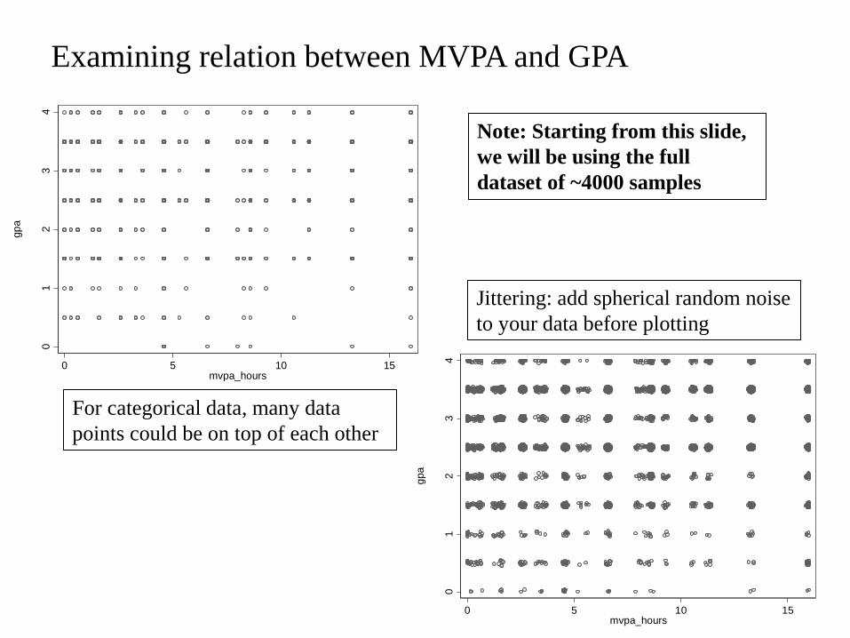
Examining relation between MVPA and GPA 0
12
34
gp
a
0 5 10 15mvpa_hours
For categorical data, many data
points could be on top of each other
Jittering: add spherical random noise
to your data before plotting
01
23
4
gpa
0 5 10 15mvpa_hours
Note: Starting from this slide,
we will be using the full
dataset of ~4000 samples
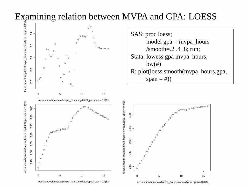
Examining relation between MVPA and GPA: LOESS
SAS: proc loess;
model gpa = mvpa_hours
/smooth=.2 .4 .8; run;
Stata: lowess gpa mvpa_hours,
bw(#)
R: plot(loess.smooth(mvpa_hours,gpa,
span = #))
0 5 10 15
2.8
02
.85
2.9
02
.95
3.0
0
loess.smooth(mydata$mvpa_hours, mydata$gpa, span = 0.8)$x
loe
ss.s
mo
oth
(myd
ata
$m
vp
a_
ho
urs
, m
yd
ata
$g
pa
, sp
an
= 0
.8)$
y
0 5 10 15
2.7
52
.80
2.8
52
.90
2.9
53
.00
3.0
5
loess.smooth(mydata$mvpa_hours, mydata$gpa, span = 0.4)$x
loe
ss.s
mo
oth
(myd
ata
$m
vp
a_
ho
urs
, m
yd
ata
$g
pa
, sp
an
= 0
.4)$
y
0 5 10 15
2.7
2.8
2.9
3.0
3.1
loess.smooth(mydata$mvpa_hours, mydata$gpa, span = 0.2)$x
loe
ss.s
mo
oth
(myd
ata
$m
vp
a_
ho
urs
, m
yd
ata
$g
pa
, sp
an
= 0
.2)$
y

LOESS (LOWESS): Deciding what to do
• LOESS provides some indication that there may be a leveling off of the
relationship between MVPA and GPA up near 10 hours/week.
• The main drawback of LOESS is there is no equation that comes out of it.
There are no coefficients (i.e. parameters) that can be tested and used to
describe the relationships. There is only the PLOT.
• Using this LOESS information along with substantive knowledge about
Physical Activity guidelines, the researchers decided to CUT the MVPA
hours into categories: e.g., < 2.5 hours per week, 2.5 − 7 hours per week,
and > 7 hours per week. This 3 category variable was then used as the
predictor rather than MVPA_HOURS.

Different strategies for deciding where to make cut points
1. Use substantive knowledge as cut points
2. Use equal spacing
3. Use quantiles (e.g. quartiles) leads to equal sizes in each category but
different interval lengths
4. Make cuts at places which can capture explicit features of nonlinearity

Testing for linear trends with categorical predictors
----------------------------------------------------------------------
mvpa_c | N(gpa) mean(gpa) sd(gpa) min(gpa) max(gpa)
----------+-----------------------------------------------------------
0- | 206 2.68932 .9122914 .5 4
2.5- | 395 2.763291 .909088 0 4
7- | 399 2.899749 .8379953 0 4
----------------------------------------------------------------------
01
23
4
gpa
0- 2.5- 7-

Test a linear CONTRAST of the coefficients
Depending on the number of levels of the categorical predictor, here are
contrasts that can be used to test for a linear trend with equally spaced
categories.
Note these can be scaled by any constant and will yield the same overall test.
Note that add to zero.

Forming and testing a contrast
SAS: data gpa_c; set gpa;
dgender = gender - 1;
mvpa_c = 0;
if mvpa_hours> 2.5 && mvpa_hours<7 then mvpa_c = 1;
if mvpa_hours>=7 then mvpa_c = 2;
run;
proc glm data = gpa_c;
class mvpa_c race;
model gpa = mvpa_c gender numcohort ses_s c_numsport race/solution;
lsmeans mvpa_c;
contrast "trend in mvpa" mvpa_c -1 0 1; ** provide Type 3 SS;
estimate "trend in mvpa" mvpa_c -1 0 1; ** provide estimated Lβ;
run;
Stata: egen mvpa_c = cut(mvpa_hours), at(0, 2.5, 7, 20) icode label
xi: reg gpa i.mvpa_c c_numsport numcohort gender ses_s i.race
lincom _Imvpa_c_2 <-- why code in this way?

SAS Output for using 3 categories for MVPA Sum of
Source DF Squares Mean Square F Value Pr > F
Model 11 353.247426 32.113402 46.81 <.0001
Error 4103 2815.043947 0.686094
Corrected Total 4114 3168.291373
R-Square Coeff Var Root MSE gpa Mean
0.111495 29.44443 0.828308 2.813123
Source DF Type III SS Mean Square F Value Pr > F
mvpa_c 2 11.3850694 5.6925347 8.30 0.0003
(...)
Standard
Parameter Estimate Error t Value Pr > |t|
mvpa_c 0 -0.144412284 B 0.03805095 -3.80 0.0001
mvpa_c 1 -0.091447055 B 0.02989343 -3.06 0.0022
mvpa_c 2 0.000000000 B . . .
(...)
Contrast DF Contrast SS Mean Square F Value Pr > F
trend in mvpa 1 9.88236577 9.88236577 14.40 0.0001
(from CONTRAST statement)
Standard
Parameter Estimate Error t Value Pr > |t|
trend in mvpa 0.14441228 0.03805095 3.80 0.0001
(from ESTIMATE statement)
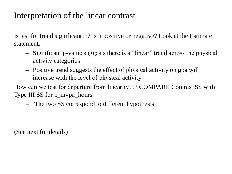
Interpretation of the linear contrast
Is test for trend significant??? Is it positive or negative? Look at the Estimate
statement.
– Significant p-value suggests there is a “linear” trend across the physical
activity categories
– Positive trend suggests the effect of physical activity on gpa will
increase with the level of physical activity
How can we test for departure from linearity??? COMPARE Contrast SS with
Type III SS for c_mvpa_hours
– The two SS correspond to different hypothesis
(See next for details)

Contrast coefficients
• Suppose X is a categorical variable with k categories: x1, …, xk
The corresponding mean outcomes in each category: μ1, …, μk
(Note that μi corresponds to the estimated coefficient for dummy variable
of ith category)
• We would like to test for a linear trend:
H0: μ1 = … = μk vs Ha: μi = β0 + β1xi, β1 ≠ 0
i.e., the points (x1, μ1), …, (xk, μk) fall along a straight line with non-zero
slope.
• Alternative, we define the contrast coefficients:
and test the hypothesis:
(Recall: what’s the estimated slope between μx and Cx?)
1, where /x i kC x x x x x k
0 0
1 1
: 0 : 0k k
x x x x
x x
H C vs H C

Contrast coefficient (cont.)
• Regress μx and Cx, the slope: (recall the formula from simple linear regression)
Therefore:
• If we fit a line through the parameter estimates, the linear contrast is to test
whether the slope of the line is zero or not.
• If we want to further test deviation from the line, we can add the categorical
variable to the model as both a continuous variable and a set of dummy
variables, e.g.,
. xi: reg gpa mvpa_c i.mvpa_c ...
and then test the significance of the dummy variables:
. testparm _Imvpa*
* 1 1
1 1
1 1
0
k k
kx x x xx xxk k x
x x x xx x
C CC
C C C C C C
*
110 0
k
x xxC

Line through adjusted means The GLM Procedure
Least Squares Means
mvpa_c gpa LSMEAN
0 2.59329550
1 2.64626073
2 2.73770778
2.5
52.6
2.6
52.7
2.7
5
GP
A (
adju
ste
d m
ean
s)
0 1 2mvpa
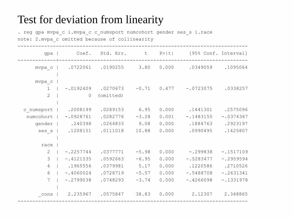
Test for deviation from linearity . reg gpa mvpa_c i.mvpa_c c_numsport numcohort gender ses_s i.race
note: 2.mvpa_c omitted because of collinearity
------------------------------------------------------------------------------
gpa | Coef. Std. Err. t P>|t| [95% Conf. Interval]
-------------+----------------------------------------------------------------
mvpa_c | .0722061 .0190255 3.80 0.000 .0349059 .1095064
|
mvpa_c |
1 | -.0192409 .0270673 -0.71 0.477 -.0723075 .0338257
2 | 0 (omitted)
|
c_numsport | .2008199 .0289153 6.95 0.000 .1441301 .2575096
numcohort | -.0928761 .0282776 -3.28 0.001 -.1483155 -.0374367
gender | .240398 .0264833 9.08 0.000 .1884763 .2923197
ses_s | .1208151 .0111018 10.88 0.000 .0990495 .1425807
|
race |
2 | -.2257744 .0377771 -5.98 0.000 -.299838 -.1517109
3 | -.4121535 .0592663 -6.95 0.000 -.5283477 -.2959594
4 | .1965556 .0379981 5.17 0.000 .1220586 .2710526
6 | -.4060024 .0728719 -5.57 0.000 -.5488708 -.2631341
7 | -.2799038 .0748293 -3.74 0.000 -.4266098 -.1331978
|
_cons | 2.235967 .0575847 38.83 0.000 2.12307 2.348865
------------------------------------------------------------------------------

Model assumptions for linear regression
• The random error ε is independent and identically distributed with:
– E(ε) = 0
– var(ε) = σ2 (equal variance)
• Linearity: the mean of Y, E(Y|X), is Xβ (i.e., the mean model is correctly
specified)
• Normality: ε ~ N(0, σ2)

Model diagnostics: residuals • “raw” Residual:
• Standardized residual:
i.e., zi is approximately unit-independent.
• Studentized residual:
where hii = ith element on the diagonal of H matrix (leverage for ith sample).
• Jackknife residual:
where is an estimate of σ2, with ith sample deleted.
• PRESS residual:
where is the fitted value of ith outcome based on all samples without ith one.
(also called prediction error, useful for outlier detection).
2
ˆ ( )
ˆ 0
T
e Y Y I H Y
E e E Y Y
V e I H V Y I H I H
, 1ˆ
ii i
ez V z
1/2
, 0, 1ˆ 1
ii i i
ii
er E r V r
h
1/2
, 0, 1ˆ 1
ii ii
iii
er E r V r
h
2ˆi
ˆ
ii i i ie Y Y
ˆi i
Y
Linearity
• Treating a variable as categorical, then plot the estimated coefficients
against their category-specific means.
– Linear trend test (see the GPA vs MVPA example)
• LOESS plot: only for simple linear regression
– Nonparametric, “approximate the regression line under the weaker
assumption that it is smooth but not necessarily linear”
– Weakness:
• Need high-dimension plot for multiple predictors
• Nonparametric smoothers work less well in higher dimensions
• Instead of checking the predictors, we can check the residuals from
multiple regression

Linearity: RVP plot
• Residual versus predictor (RVP) plot: plot ei vs. each covariate Xj
– If relationship between Xj and E[Y] modeled correctly, plot should be a
random scatter.
– Trend in plot may suggest modifications to model.
– Weakness: ei accounts for contribution of other covariates – can’t see
“correct” relationship between each Xj and E[Y].
-3-2
-10
12
Resid
uals
0 5 10 15mvpa_hours
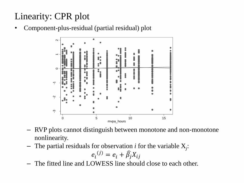
Linearity: CPR plot
• Component-plus-residual (partial residual) plot
– RVP plots cannot distinguish between monotone and non-monotone
nonlinearity.
– The partial residuals for observation i for the variable Xj:
𝑒𝑖(𝑗) = 𝑒𝑖 + 𝛽𝑗 𝑋𝑖𝑗
– The fitted line and LOWESS line should close to each other.
-3-2
-10
12
Com
pon
en
t plu
s r
esid
ual
0 5 10 15mvpa_hours
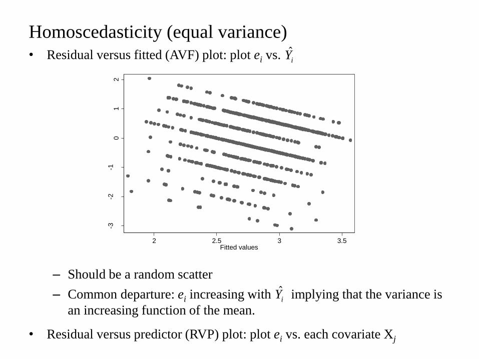
Homoscedasticity (equal variance)
• Residual versus fitted (AVF) plot: plot ei vs.
– Should be a random scatter
– Common departure: ei increasing with implying that the variance is
an increasing function of the mean.
• Residual versus predictor (RVP) plot: plot ei vs. each covariate Xj
ˆiY
ˆiY
-3-2
-10
12
Re
sid
ua
ls
2 2.5 3 3.5Fitted values

Homoscedasticity: statistical tests
• Formal statistical tests:
1. Breusch-Pagan (or Godfrey or Lagrange Multiplier) test. The basic idea
is to examine whether there is some variation in the squared residuals
which can be explained by variation in the predictor variables. Breusch-
Pagan tests the hypothesis that , where Z is a subset
and/or function of predictors in X. The model is homoscedastic if α = 0.
The null hypothesis being tested is that α = 0, so rejecting using this test
implies heteroscedasticity. Could perform this test by explicitly doing the
regression of the squared residuals. • SAS: use PROC MODEL and the /breusch option for the fit command.
• Stata: -bpagan- (user-written command) or -estat hettest- (newer version).
2. White’s general test. Basically a special case of the Breusch-Pagan test.
For White’s test, the Z considers all possible first and second order
combinations of predictors. The null hypothesis is homoscedasticity, so
rejecting implies heteroscedasticity. • SAS: use /spec in model statement of PROC REG to get White’s test. Can also
use PROC MODEL and the /white option for the fit command.
• Stata: -whitetst- (user-written command) or -estat imtest, white- (newer version).

Fixes or ways to account for heteroscedasticity
• Given a known model for the heteroscedasticity, use this to form weighted
least squares (WLS) estimator. Given known values for variance-
covariance (Ω), can use “weight” statement in most SAS PROCs or Stata
commands.
– Pros: estimator of β is more efficient than OLS and standard errors are
correct.
– Cons: Often don’t know Ω.
• Empirically model the heteroscedasticity (e.g. using regression formula
considered in Breusch-Pagan test), obtain predicted values from regression
which are estimates of σ2 . Use these estimates to form Ω and plug this in to
WLS, called the Feasible weighted least squares (FWLS) estimator. Also
called FGLS (feasible generalized least squares).
– Pros: provides a way to directly estimate heteroscedasticity and
asymptotically is equivalent to WLS if Ω is a consistent estimator of Ω.
– Cons: modeling error variance introduces more complexity, need to be
careful to delineate what is important for the mean verses what explains
the variability.
Fixes or ways to account for heteroscedasticity
• Use a variance stabilizing transformation, then proceed with OLS. That is,
take the log or square root of the outcome variable and/or predictors.
– Pros: simple.
– Cons: when results need to be interpreted on the original scale, not
always straightforward how to back-transform.
• Use robust standard errors or “heteroscedastic consistent (HC) standard
errors”. Continue to use OLS since it is unbiased even in the presence of
heteroscedasticity, but use a “robust” standard error estimator. This is called
the White, Eicker or Huber estimator.
– Pros: easy to implement without need to have a model for
heteroscedasticity.
– Cons: No specific obvious cons, but it is still important to look for
systematic reasons (mean model mis-specification) for why there is
heteroscedasticity in the first place.
SAS: use Proc REG with the /ACOV option
Stata: use the –vce(robust)- option
• Carefully examine for mis-specification of the mean model. Missing
covariates, or interactions, or nonlinear predictors can lead to what appears
to be heteroscedastic errors.
Independence
• Carefully check study design for potential correlation between observations
– e.g., time-ordered (serial correlation), cluster data, repeated measures
• Checking for autocorrelation:
– Plot ei vs time
– Plot ei vs ei-1
– Runs test: check sequence of time-ordered ei with same sign
– Durbin-Watson test: AR-1 correlation
• Cluster data:
– Long format: one-way ANOVA
– Wide format: Pearson correlation coefficient
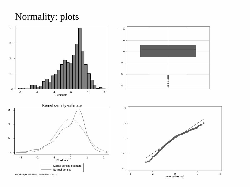
Normality
• Histogram of residuals
– Should be symmetric, bell-shaped, light-tailed
• Box/whisker plot
– 25th and 75th percentiles should be equally distant from median
– More useful than histogram when n low
• Summary statistics
– Median should close to mean
• Q-Q plot
• Formal statistical tests, e.g., Shapiro-Wilks test
– Such tests are often sensitive to sample size: “often failing to reject the
null hypothesis of normality in small samples where meeting this
assumption is most important, and conversely rejecting it even for
small violations in large data sets where inferences are relatively robust
to departures from normality.”
Normality: plots 0
.2.4
.6.8
De
nsity
-3 -2 -1 0 1 2Residuals
-3-2
-10
12
Re
sid
ua
ls
0.2
.4.6
De
nsity
-3 -2 -1 0 1 2Residuals
Kernel density estimate
Normal density
kernel = epanechnikov, bandwidth = 0.1772
Kernel density estimate
-4-2
02
4
Re
sid
ua
ls
-4 -2 0 2 4Inverse Normal
Outliers and influential observations
• An observation can be outlying in the outcome or the predictor variables.
• An outlying observation can appear not to be outlying when looking only
marginally at any of the variables, but can be found to be outlying in terms
of not being well described by the model relating the variables to one
another.
• Outlier: data with unusually large residuals.
– Model fit could be poor at outlier points.
– May have disproportionately great influence on estimates
– May not represent target population
• Residuals can be examined to detect outliers that are not well described by
the data.
– Standardized residuals, e.g. > 3 or < −3 might be considered for further
examination.
• Influential observations are those that have high leverage (i.e. outlying in
the x variable) and thus have potential to change parameter estimates
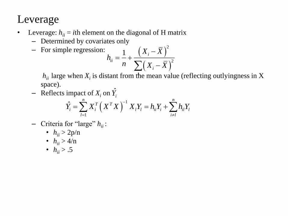
Leverage • Leverage: hii = ith element on the diagonal of H matrix
– Determined by covariates only
– For simple regression:
hii large when Xi is distant from the mean value (reflecting outlyingness in X
space).
– Reflects impact of Xi on
– Criteria for “large” hii :
• hii > 2p/n
• hii > 4/n
• hii > .5
2
2
1 i
ii
i
i
X Xh
n X X
1
1
ˆn n
T T
i i l l ii i il l
l i l
Y X X X X Y h Y h Y
ˆiY
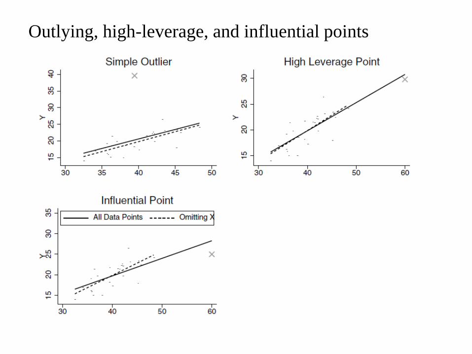
Outlying, high-leverage, and influential points
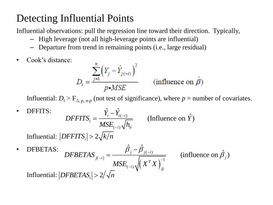
Detecting Influential Points Influential observations: pull the regression line toward their direction. Typically,
– High leverage (not all high-leverage points are influential)
– Departure from trend in remaining points (i.e., large residual)
• Cook’s distance:
Influential: Di > F.5, p, n-p (not test of significance), where p = number of covariates.
• DFFITS:
Influential:
• DFBETAS:
Influential:
( )
( )
ˆ ˆˆ(Influence on )
i i i
i
i ii
Y YDFFITS Y
MSE h
2iDFFITS k n
( )
1
( )
ˆ ˆˆ(influence on )
j j i
jj iT
i jj
DFBETAS
MSE X X
2iDFBETAS n

DFBETAS (corresponding to the three scenarios described
previously)

Outliers: added variable plot
• Added variable (partial-regression leverage) plot:
– Set X = [Xj , X-j ], where X-j contains all covariates except Xj .
• Set e(Y| X-j ) as the residuals for Y regressed on X-j .
• Set e(Xj | X-j ) as the residuals for Xj regressed on X-j .
– Plot e(Y| X-j ) vs e(Xj | X-j )
• Both sets of residuals are covariate-adjusted.
• Project multidimensional data back to the two-dimensional world
-3-2
-10
12
e(
gpa
| X
)
-10 -5 0 5 10 15e( mvpa_hours | X )
coef = .00617867, se = .00603294, t = 1.02

Fixes to outliers and influential observations • Check for mistake in data entry, also ask yourself whether observation is not
actually in target population
• If outlier is a legitimate value, need to decide whether to keep in or delete – can do sensitivity analysis and report varying results.
• Robust regression. Robust regression is a compromise between deleting the outlying points, and allowing them to violate the assumptions of OLS regression. It is a kind of weighted least squares regression where the weights are inversely related to the residuals. There are several different methods for weighting...SAS version 9 uses PROC ROBUSTREG, Stata uses -rreg-.
• Robust regression is more computationally intensive than OLS but is likely to become more and more popular now that SAS and other statistical software implement it.
• Note: Robust standard errors address the problem of errors that are not independent and identically distributed and do not change the coefficient estimates provided by OLS (or ML), but only change the standard errors and significance tests. Robust regression uses a weighting scheme that causes outliers to have less impact on the estimates of regression coefficients, hence producing different coefficient estimates (and likewise standard errors) than OLS does.
Collinearity
• Collinearity or “multicollinearity” denotes correlation between predictors
high enough to make the standard errors of the regression coefficient
estimates become large.
• Not necessarily a problem:
1. if only interested in prediction, collinearity is not likely to increase
prediction error
2. if collinearity exists between “control variables”, not likely to affect
parameter estimates for target predictors.
• Collinearity usually pops up as a “problem” when we have a target
predictor or several potential target predictors which we would expect to
find significantly related to the outcome, but when they are included in the
multiple regression (possibly with control variables) they are not significant
(with large standard errors). This is most likely happening because the
predictors are highly correlated with one another or else highly correlated
with control variable(s), i.e. because of collinearity.

Multicollinearity: VIF
• In OLS, variance of estimated coefficient can be expressed as:
where Rj2 is the multiple R2 for the regression of Xj on the other covariates.
• Variance inflation factor (VIF):
reflects all other covariates that influence the uncertainty in the coefficient
estimates. As a rule of thumb, a variable whose VIF values is greater than
10 may merit further investigation.
• Also can look for large Pearson correlations between predictors.
2
2
1ˆ11 var
j
jj
VarRn X
2
1ˆ1
j
j
VIFR

Fixes to Multicollinearity
• Examine whether there are some redundant variables (i.e. variables
measuring essentially the same thing) and choose to eliminate them.
• If meaningful, create composite variable from those that are highly
correlated.
• Carefully consider causal reasoning for including variables and potentially
drop if in causal pathway.
• Accept answer as is, finding the target predictor NOT being significant may
indeed be the right answer (if the effect is truly being confounded)
• “Admit that data are inadequate to disentangle their effects” (Vittinghoff et
al.) due to their strong correlation

Review: Linear regression model
• Simple and multiple linear regression
• Ordinary least squares
• Interpreting regression coefficients - continuous versus categorical
• Testing regression coefficients, F-test and t-test, standard errors, MSE
• Understanding effect of correlation between predictors on regression
coefficients (confounding, mediation, etc.)
• Effect of centering and standardizing variables
• Fitted values, Adjusted means (“least square means”)
• R2 interpretation
• Interaction: interpretation of coefficients for the interaction
• LOESS plot
• Test for linear trend
• Model assumptions and model diagnostics