Embed Size (px)
Citation preview
General Introduction to
Parallel Computing
Rezaul ChowdhuryDepartment of Computer Science
Stony Brook University
Why Parallelism?

Moore’s Law
Source: Wikipedia

Unicore Performance
Source: Jeff Preshing, 2012, http://preshing.com/20120208/a-look-back-at-single-threaded-cpu-performance/
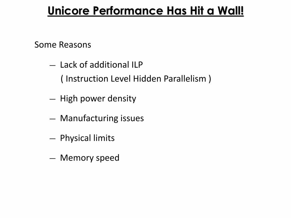
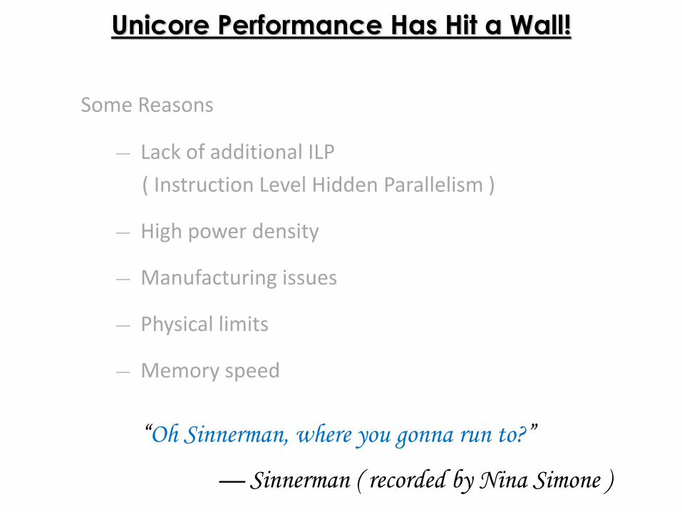
Unicore Performance Has Hit a Wall!
Some Reasons
― Lack of additional ILP
( Instruction Level Hidden Parallelism )
― High power density
― Manufacturing issues
― Physical limits
― Memory speed
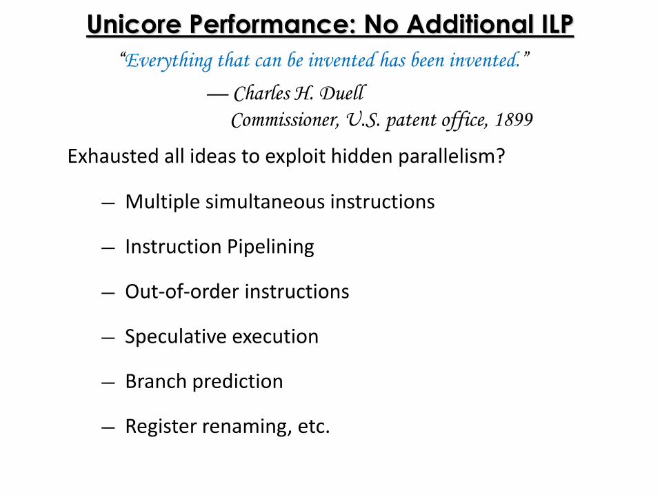
Unicore Performance: No Additional ILP
Exhausted all ideas to exploit hidden parallelism?
― Multiple simultaneous instructions
― Instruction Pipelining
― Out-of-order instructions
― Speculative execution
― Branch prediction
― Register renaming, etc.
“Everything that can be invented has been invented.”
— Charles H. Duell
Commissioner, U.S. patent office, 1899
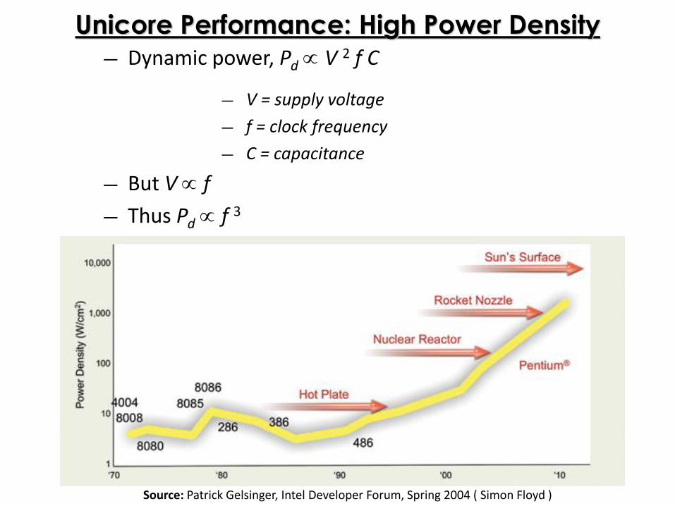
Unicore Performance: High Power Density― Dynamic power, Pd V 2 f C
― V = supply voltage
― f = clock frequency
― C = capacitance
― But V f
― Thus Pd f 3
Source: Patrick Gelsinger, Intel Developer Forum, Spring 2004 ( Simon Floyd )
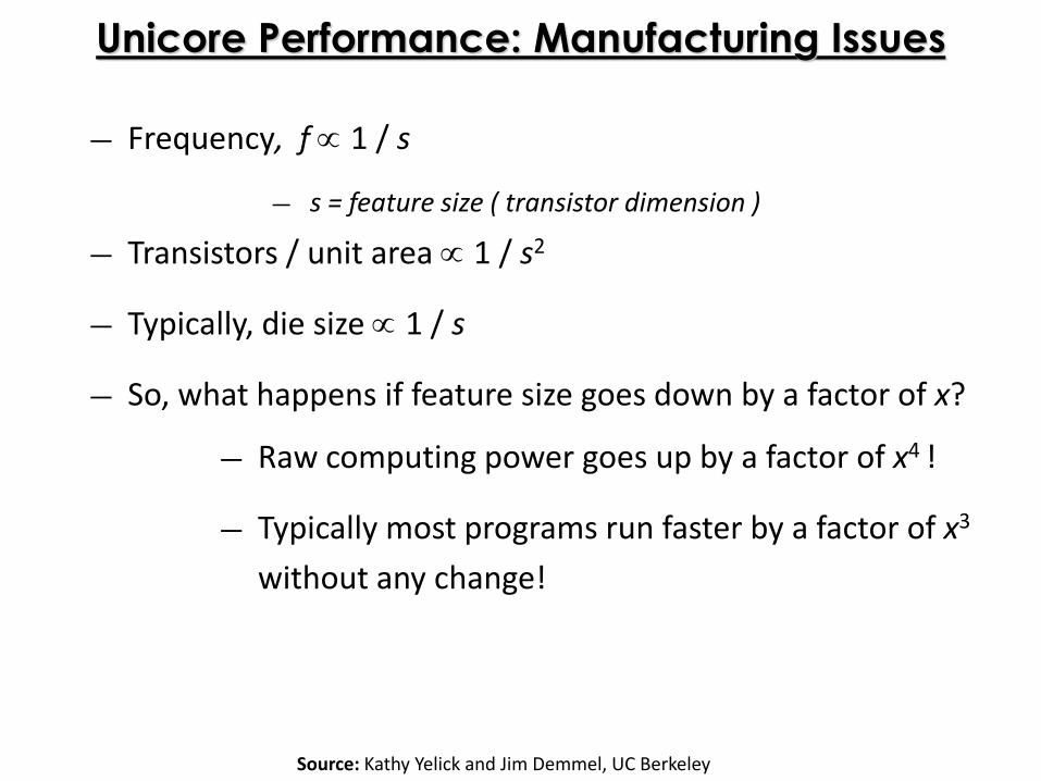
Unicore Performance: Manufacturing Issues
― Frequency, f 1 / s
― s = feature size ( transistor dimension )
― Transistors / unit area 1 / s2
― Typically, die size 1 / s
― So, what happens if feature size goes down by a factor of x?
― Raw computing power goes up by a factor of x4 !
― Typically most programs run faster by a factor of x3
without any change!
Source: Kathy Yelick and Jim Demmel, UC Berkeley

Unicore Performance: Manufacturing Issues
― Manufacturing cost goes up as feature size decreases
― Cost of a semiconductor fabrication plant doubles
every 4 years ( Rock’s Law )
― CMOS feature size is limited to 5 nm ( at least 10 atoms )
Source: Kathy Yelick and Jim Demmel, UC Berkeley
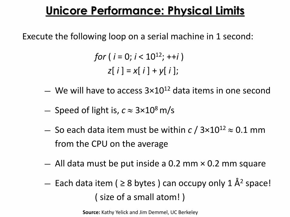
Unicore Performance: Physical Limits
Execute the following loop on a serial machine in 1 second:
for ( i = 0; i < 1012; ++i )
z[ i ] = x[ i ] + y[ i ];
― We will have to access 3×10¹² data items in one second
― Speed of light is, c 3×10⁸ m/s
― So each data item must be within c / 3×10¹² 0.1 mm
from the CPU on the average
― All data must be put inside a 0.2 mm × 0.2 mm square
― Each data item ( ≥ 8 bytes ) can occupy only 1 Å2 space!
( size of a small atom! )
Source: Kathy Yelick and Jim Demmel, UC Berkeley
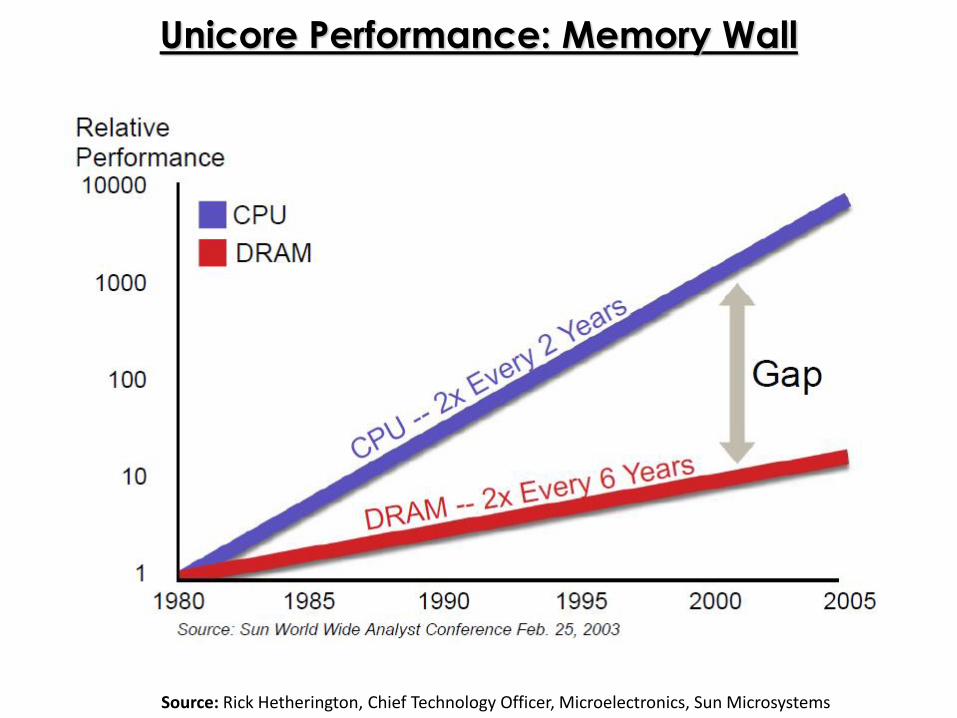
Unicore Performance: Memory Wall
Source: Rick Hetherington, Chief Technology Officer, Microelectronics, Sun Microsystems
Unicore Performance Has Hit a Wall!
Some Reasons
― Lack of additional ILP
( Instruction Level Hidden Parallelism )
― High power density
― Manufacturing issues
― Physical limits
― Memory speed
“Oh Sinnerman, where you gonna run to?”
— Sinnerman ( recorded by Nina Simone )

Where You Gonna Run To?
― Changing f by 20% changes performance by 13%
― So what happens if we overclock by 20%?
Source: Andrew A. Chien, Vice President of Research, Intel Corporation

― Changing f by 20% changes performance by 13%
― So what happens if we overclock by 20%?
― And underclock by 20%?
Source: Andrew A. Chien, Vice President of Research, Intel Corporation
Where You Gonna Run To?

― Changing f by 20% changes performance by 13%
― So what happens if we overclock by 20%?
― And underclock by 20%?
Source: Andrew A. Chien, Vice President of Research, Intel Corporation
Where You Gonna Run To?
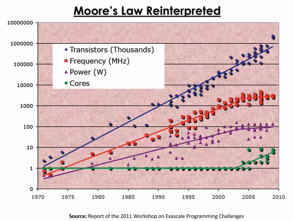
Moore’s Law Reinterpreted
Source: Report of the 2011 Workshop on Exascale Programming Challenges
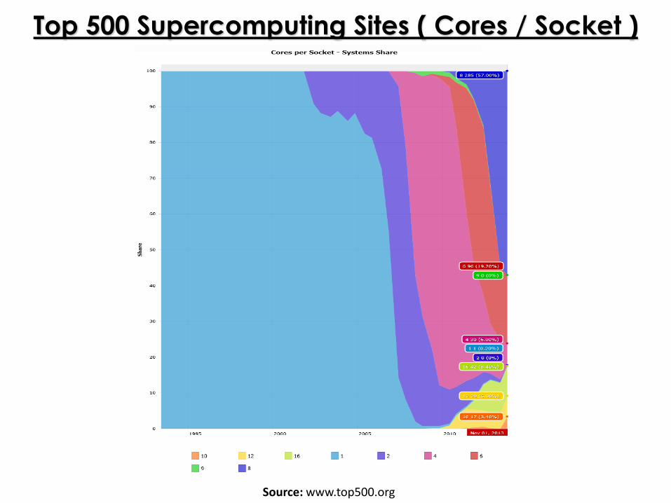
Source: www.top500.org
Top 500 Supercomputing Sites ( Cores / Socket )
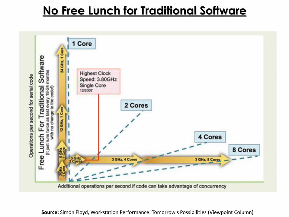
No Free Lunch for Traditional Software
Source: Simon Floyd, Workstation Performance: Tomorrow's Possibilities (Viewpoint Column)
A Useful Classification
of Parallel Computers
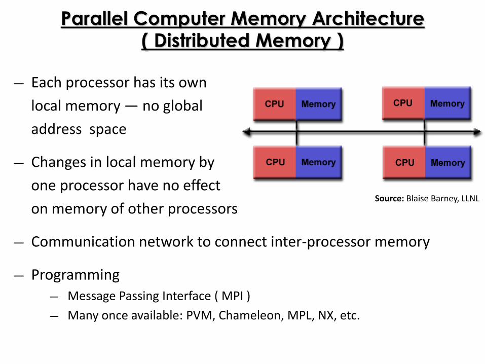
Parallel Computer Memory Architecture( Distributed Memory )
― Each processor has its own
local memory ― no global
address space
― Changes in local memory by
one processor have no effect
on memory of other processors
― Communication network to connect inter-processor memory
― Programming
― Message Passing Interface ( MPI )
― Many once available: PVM, Chameleon, MPL, NX, etc.
Source: Blaise Barney, LLNL
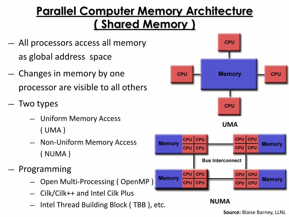
Parallel Computer Memory Architecture( Shared Memory )
― All processors access all memory
as global address space
― Changes in memory by one
processor are visible to all others
― Two types
― Uniform Memory Access
( UMA )
― Non-Uniform Memory Access
( NUMA )
― Programming
― Open Multi-Processing ( OpenMP )
― Cilk/Cilk++ and Intel Cilk Plus
― Intel Thread Building Block ( TBB ), etc.
UMA
NUMA
Source: Blaise Barney, LLNL
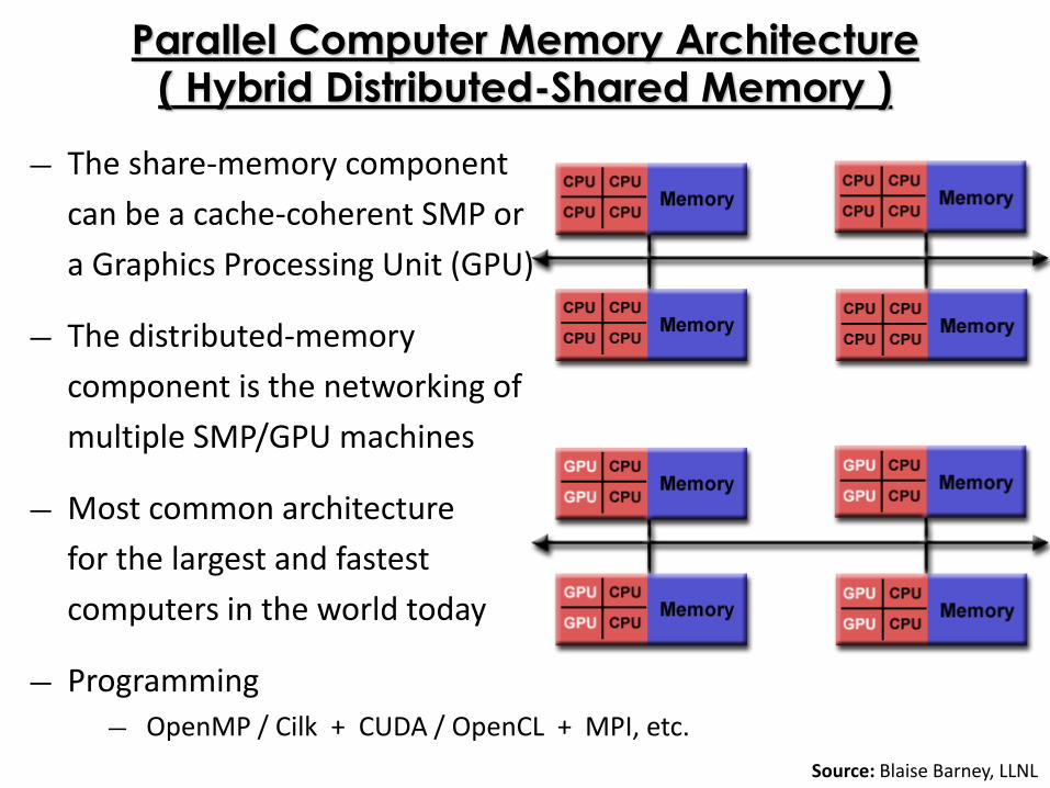
Parallel Computer Memory Architecture( Hybrid Distributed-Shared Memory )
― The share-memory component
can be a cache-coherent SMP or
a Graphics Processing Unit (GPU)
― The distributed-memory
component is the networking of
multiple SMP/GPU machines
― Most common architecture
for the largest and fastest
computers in the world today
― Programming
― OpenMP / Cilk + CUDA / OpenCL + MPI, etc.
Source: Blaise Barney, LLNL

Types of Parallelism
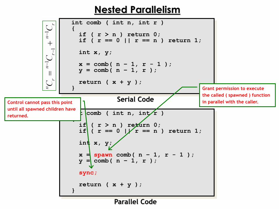
Nested Parallelismint comb ( int n, int r ) {
if ( r > n ) return 0;if ( r == 0 || r == n ) return 1;
int x, y;
x = comb( n – 1, r - 1 );y = comb( n – 1, r );
return ( x + y );}
int comb ( int n, int r ) {
if ( r > n ) return 0;if ( r == 0 || r == n ) return 1;
int x, y;
x = spawn comb( n – 1, r - 1 );y = comb( n – 1, r );
sync;
return ( x + y );}
Grant permission to execute
the called ( spawned ) function
in parallel with the caller.Control cannot pass this point
until all spawned children have
returned.
Serial Code
Parallel Code
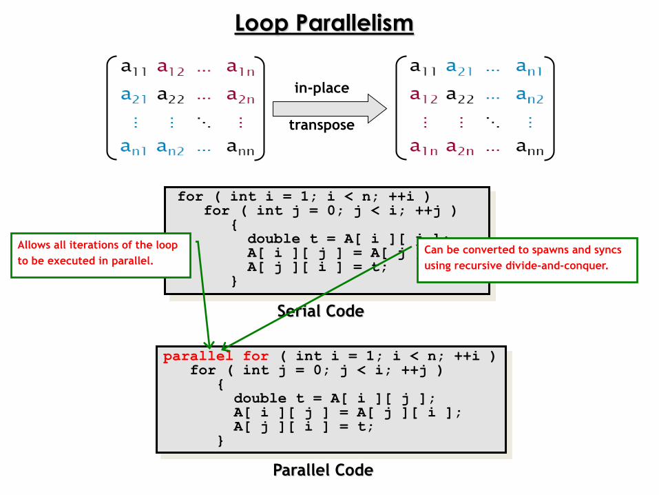
Loop Parallelism
in-place
transpose
for ( int i = 1; i < n; ++i )for ( int j = 0; j < i; ++j )
{double t = A[ i ][ j ];A[ i ][ j ] = A[ j ][ i ]; A[ j ][ i ] = t;
}
Serial Code
parallel for ( int i = 1; i < n; ++i )for ( int j = 0; j < i; ++j )
{double t = A[ i ][ j ];A[ i ][ j ] = A[ j ][ i ]; A[ j ][ i ] = t;
}
Parallel Code
Allows all iterations of the loop
to be executed in parallel.Can be converted to spawns and syncs
using recursive divide-and-conquer.

Analyzing
Parallel Algorithms
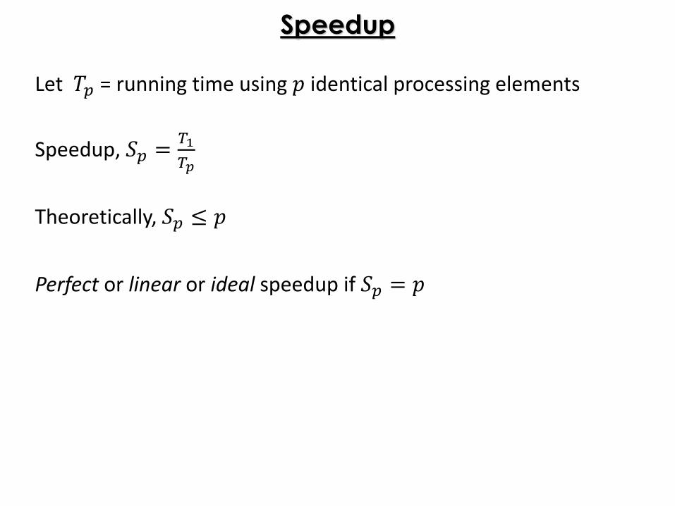
Speedup
Speedup, 𝑆𝑝 =𝑇1
𝑇𝑝
Let 𝑇𝑝 = running time using 𝑝 identical processing elements
Theoretically, 𝑆𝑝 ≤ 𝑝
Perfect or linear or ideal speedup if 𝑆𝑝 = 𝑝
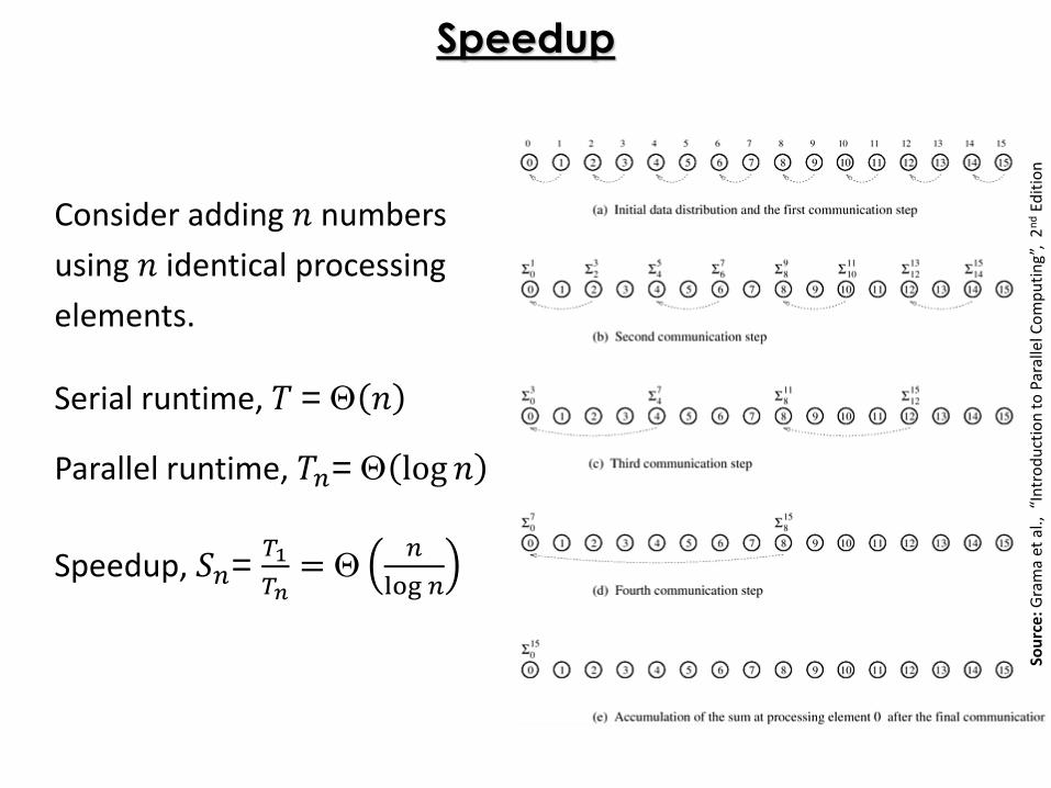
Speedup
Sou
rce:
Gra
ma
et a
l., “
Intr
od
uct
ion
to
Par
alle
l Co
mp
uti
ng”
, 2
nd
Edit
ion
Consider adding 𝑛 numbers
using 𝑛 identical processing
elements.
Serial runtime, 𝑇 = 𝑛
Parallel runtime, 𝑇𝑛= log 𝑛
Speedup, 𝑆𝑛= 𝑇1
𝑇𝑛=
𝑛
log 𝑛
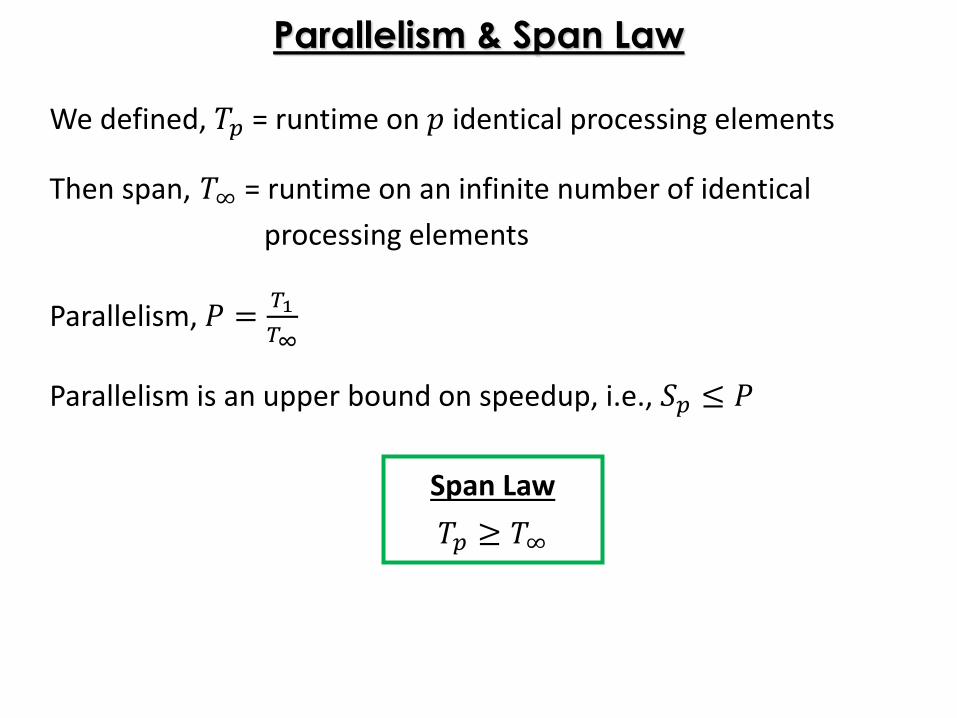
Parallelism & Span Law
Parallelism, 𝑃 =𝑇1
𝑇∞
We defined, 𝑇𝑝 = runtime on 𝑝 identical processing elements
Parallelism is an upper bound on speedup, i.e., 𝑆𝑝 ≤ 𝑃
Then span, 𝑇∞ = runtime on an infinite number of identical
processing elements
Span Law
𝑇𝑝 ≥ 𝑇∞
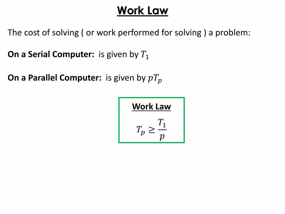
Work Law
The cost of solving ( or work performed for solving ) a problem:
On a Serial Computer: is given by 𝑇1
On a Parallel Computer: is given by 𝑝𝑇𝑝
Work Law
𝑇𝑝 ≥𝑇1𝑝
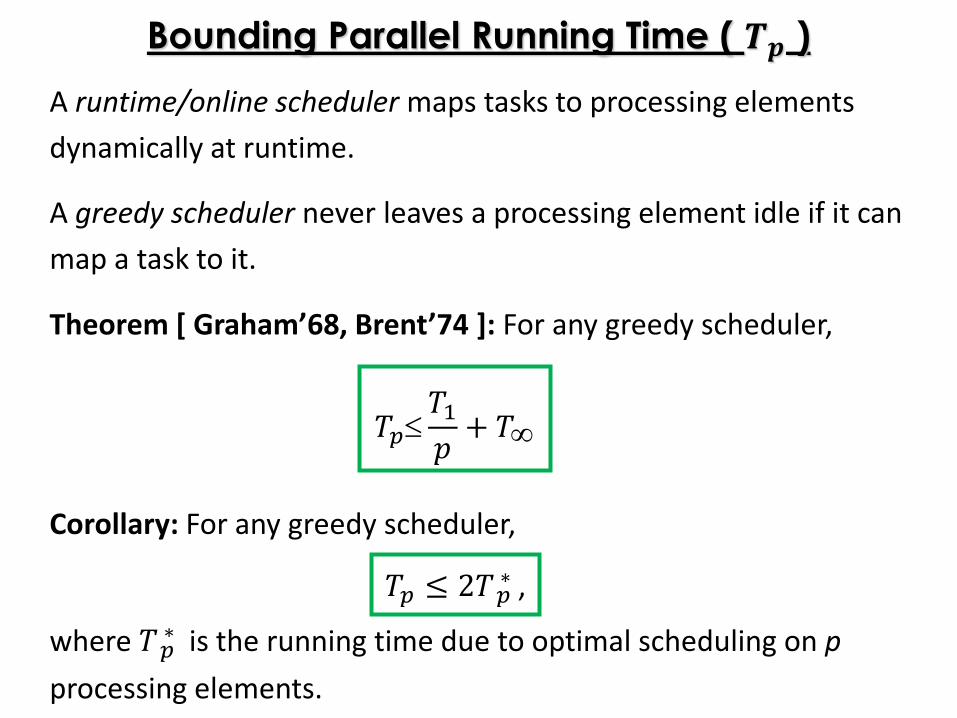
A runtime/online scheduler maps tasks to processing elements
dynamically at runtime.
A greedy scheduler never leaves a processing element idle if it can
map a task to it.
Bounding Parallel Running Time ( 𝑻𝒑 )
Theorem [ Graham’68, Brent’74 ]: For any greedy scheduler,
𝑇𝑝𝑇1𝑝+ 𝑇
Corollary: For any greedy scheduler,
where 𝑇𝑝∗ is the running time due to optimal scheduling on p
processing elements.
𝑇𝑝 ≤ 2𝑇𝑝∗ ,
Analyzing Parallel
Matrix Multiplication
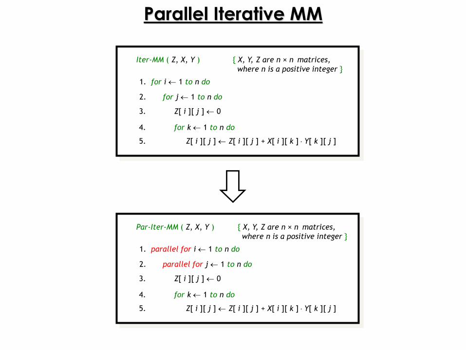
Iter-MM ( Z, X, Y ) { X, Y, Z are n × n matrices,
where n is a positive integer }
1. for i 1 to n do
3. Z[ i ][ j ] 0
4. for k 1 to n do
2. for j 1 to n do
5. Z[ i ][ j ] Z[ i ][ j ] + X[ i ][ k ] Y[ k ][ j ]
Parallel Iterative MM
Par-Iter-MM ( Z, X, Y ) { X, Y, Z are n × n matrices,
where n is a positive integer }
1. parallel for i 1 to n do
3. Z[ i ][ j ] 0
4. for k 1 to n do
2. parallel for j 1 to n do
5. Z[ i ][ j ] Z[ i ][ j ] + X[ i ][ k ] Y[ k ][ j ]
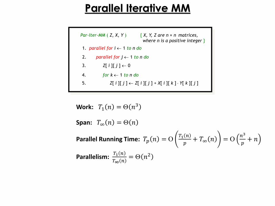
Parallel Iterative MM
Par-Iter-MM ( Z, X, Y ) { X, Y, Z are n × n matrices,
where n is a positive integer }
1. parallel for i 1 to n do
3. Z[ i ][ j ] 0
4. for k 1 to n do
2. parallel for j 1 to n do
5. Z[ i ][ j ] Z[ i ][ j ] + X[ i ][ k ] Y[ k ][ j ]
Parallelism: 𝑇1 𝑛
𝑇∞ 𝑛= 𝑛2
Work: 𝑇1 𝑛 = 𝑛3
Span: 𝑇∞ 𝑛 = 𝑛
Parallel Running Time: 𝑇𝑝 𝑛 = 𝑇1 𝑛
𝑝+ 𝑇∞ 𝑛 =
𝑛3
𝑝+ 𝑛
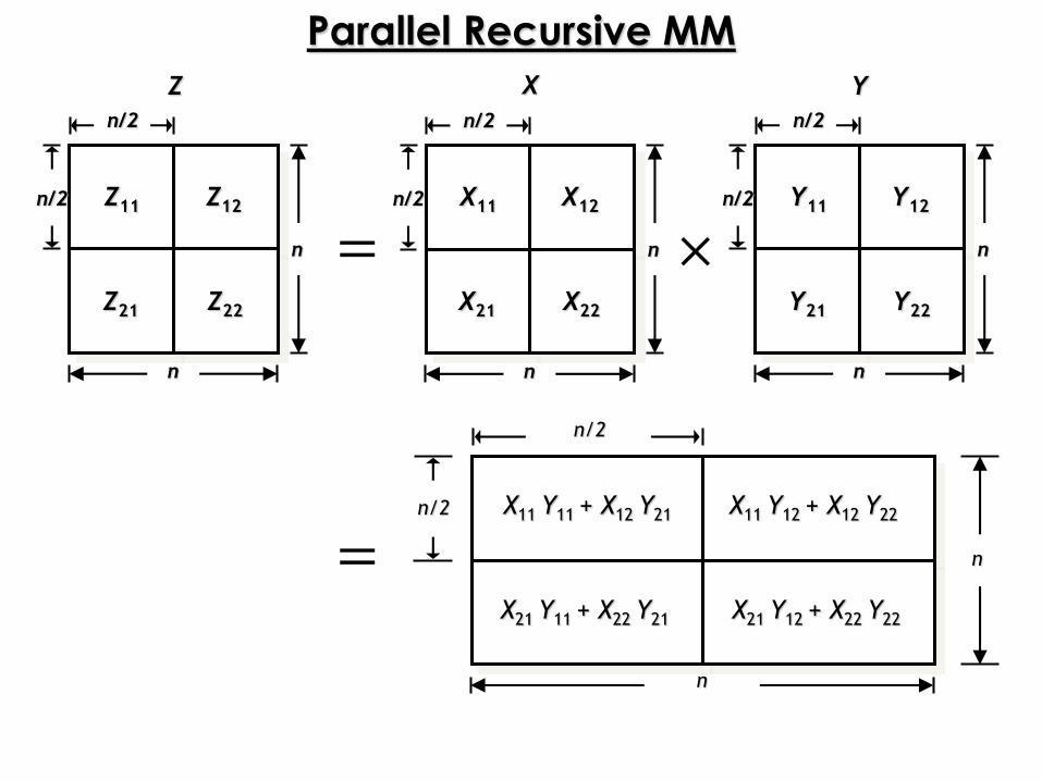
Parallel Recursive MM
Z
n
n
n/2
n/2 Z11
Z21
Z12
Z22
n
n
n/2
n/2 X11 Y11 + X12 Y21
X21 Y11 + X22 Y21
X11 Y12 + X12 Y22
X21 Y12 + X22 Y22
X Y
n
n
n/2
n/2 X11
X21
X12
X22
n
n
n/2
n/2 Y11
Y21
Y12
Y22
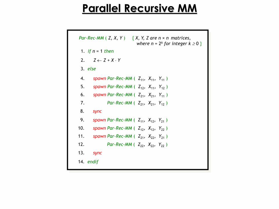
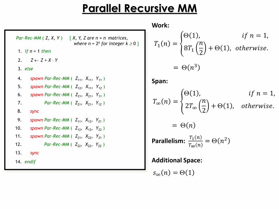
Parallel Recursive MM
Par-Rec-MM ( Z, X, Y ) { X, Y, Z are n × n matrices,
where n = 2k for integer k 0 }
1. if n = 1 then
3. else
4. spawn Par-Rec-MM ( Z11, X11, Y11 )
2. Z Z + X Y
5. spawn Par-Rec-MM ( Z12, X11, Y12 )
6. spawn Par-Rec-MM ( Z21, X21, Y11 )
7. Par-Rec-MM ( Z21, X21, Y12 )
9. spawn Par-Rec-MM ( Z11, X12, Y21 )
10. spawn Par-Rec-MM ( Z12, X12, Y22 )
11. spawn Par-Rec-MM ( Z21, X22, Y21 )
12. Par-Rec-MM ( Z22, X22, Y22 )
13. sync
14. endif
8. sync
𝑇1 𝑛 = 1 , 𝑖𝑓 𝑛 = 1,
8𝑇1𝑛
2+ 1 , 𝑜𝑡ℎ𝑒𝑟𝑤𝑖𝑠𝑒.
= 𝑛3
𝑇∞ 𝑛 = 1 , 𝑖𝑓 𝑛 = 1,
2𝑇∞𝑛
2+ 1 , 𝑜𝑡ℎ𝑒𝑟𝑤𝑖𝑠𝑒.
= 𝑛
𝑠∞ 𝑛 = 1
Parallelism: 𝑇1 𝑛
𝑇∞ 𝑛= 𝑛2
Additional Space:
Span:
Work:
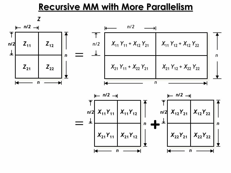
Recursive MM with More Parallelism
Z
n
n
n/2
n/2 Z11
Z21
Z12
Z22
n
n
n/2
n/2 X11Y11
X21Y11
X11Y12
X21Y12
n
n
n/2
n/2 X12Y21
X22Y21
X12Y22
X22Y22
n
n
n/2
n/2 X11 Y11 + X12 Y21
X21 Y11 + X22 Y21
X11 Y12 + X12 Y22
X21 Y12 + X22 Y22
Par-Rec-MM2 ( Z, X, Y ) { X, Y, Z are n × n matrices,
where n = 2k for integer k 0 }
1. if n = 1 then
3. else { T is a temporary n n matrix }
4. spawn Par-Rec-MM2 ( Z11, X11, Y11 )
2. Z Z + X Y
5. spawn Par-Rec-MM2 ( Z12, X11, Y12 )
6. spawn Par-Rec-MM2 ( Z21, X21, Y11 )
7. spawn Par-Rec-MM2 ( Z21, X21, Y12 )
8. spawn Par-Rec-MM2 ( T11, X12, Y21 )
9. spawn Par-Rec-MM2 ( T12, X12, Y22 )
10. spawn Par-Rec-MM2 ( T21, X22, Y21 )
11. Par-Rec-MM2 ( T22, X22, Y22 )
12. sync
13. parallel for i 1 to n do
15. Z[ i ][ j ] Z[ i ][ j ] + T[ i ][ j ]
14. parallel for j 1 to n do
16. endif
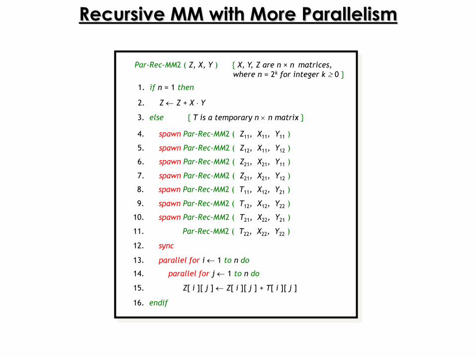
Recursive MM with More Parallelism
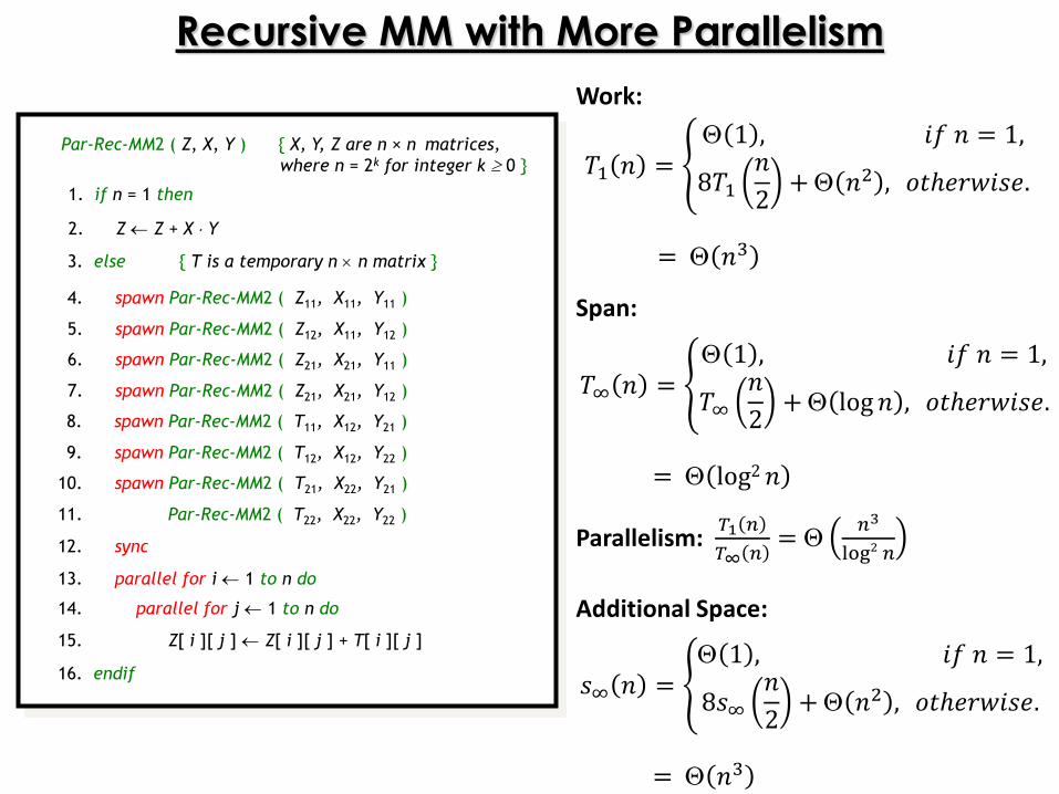
Par-Rec-MM2 ( Z, X, Y ) { X, Y, Z are n × n matrices,
where n = 2k for integer k 0 }
1. if n = 1 then
3. else { T is a temporary n n matrix }
4. spawn Par-Rec-MM2 ( Z11, X11, Y11 )
2. Z Z + X Y
5. spawn Par-Rec-MM2 ( Z12, X11, Y12 )
6. spawn Par-Rec-MM2 ( Z21, X21, Y11 )
7. spawn Par-Rec-MM2 ( Z21, X21, Y12 )
8. spawn Par-Rec-MM2 ( T11, X12, Y21 )
9. spawn Par-Rec-MM2 ( T12, X12, Y22 )
10. spawn Par-Rec-MM2 ( T21, X22, Y21 )
11. Par-Rec-MM2 ( T22, X22, Y22 )
12. sync
13. parallel for i 1 to n do
15. Z[ i ][ j ] Z[ i ][ j ] + T[ i ][ j ]
14. parallel for j 1 to n do
16. endif
𝑇1 𝑛 = 1 , 𝑖𝑓 𝑛 = 1,
8𝑇1𝑛
2+ 𝑛2 , 𝑜𝑡ℎ𝑒𝑟𝑤𝑖𝑠𝑒.
= 𝑛3
𝑇∞ 𝑛 = 1 , 𝑖𝑓 𝑛 = 1,
𝑇∞𝑛
2+ log 𝑛 , 𝑜𝑡ℎ𝑒𝑟𝑤𝑖𝑠𝑒.
= log2𝑛
𝑠∞ 𝑛 = 1 , 𝑖𝑓 𝑛 = 1,
8𝑠∞𝑛
2+ 𝑛2 , 𝑜𝑡ℎ𝑒𝑟𝑤𝑖𝑠𝑒.
= 𝑛3
Parallelism: 𝑇1 𝑛
𝑇∞ 𝑛=
𝑛3
log2 𝑛
Additional Space:
Span:
Work:
Recursive MM with More Parallelism
Distributed-Memory Naïve Matrix Multiplication
1
n
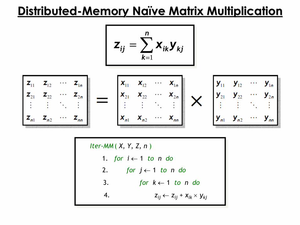
ij ik kj
k
z x y
Iter-MM ( X, Y, Z, n )
1. for i 1 to n do
2. for j 1 to n do
3. for k 1 to n do
4. zij zij + xik ykj
1
n
ij ik kj
k
z x y
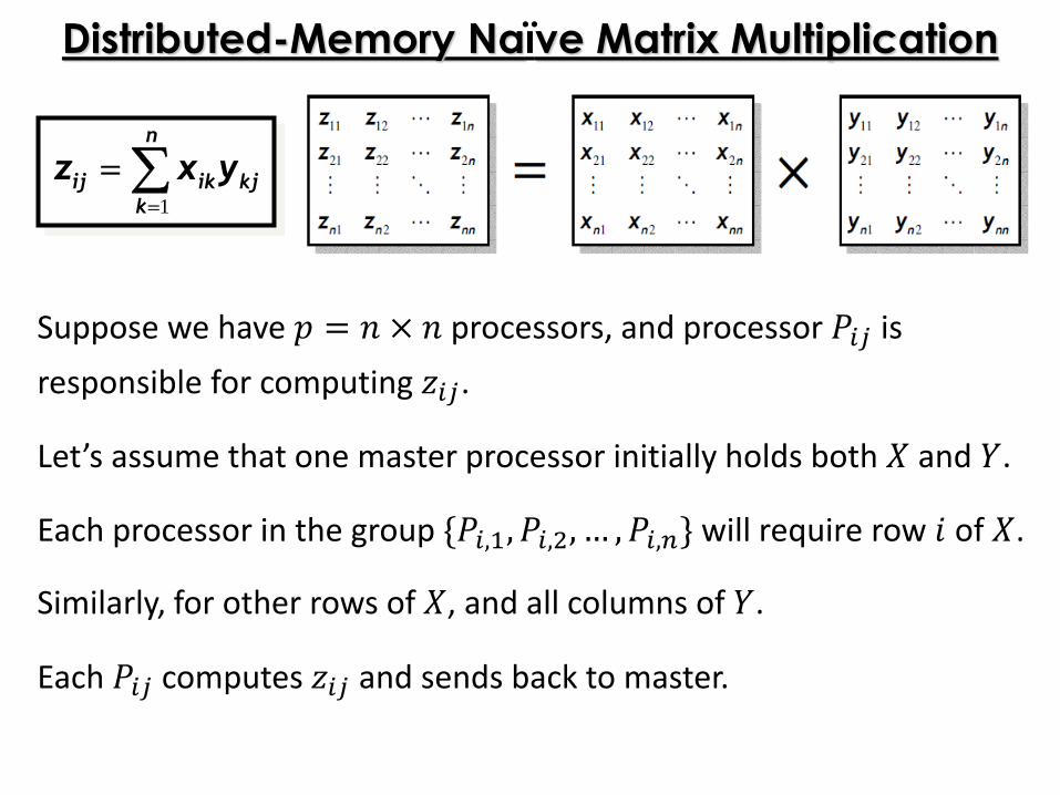
Suppose we have 𝑝 = 𝑛 × 𝑛 processors, and processor 𝑃𝑖𝑗 is
responsible for computing 𝑧𝑖𝑗.
Let’s assume that one master processor initially holds both 𝑋 and 𝑌.
Each processor in the group {𝑃𝑖,1, 𝑃𝑖,2, … , 𝑃𝑖,𝑛} will require row 𝑖 of 𝑋.
Similarly, for other rows of 𝑋, and all columns of 𝑌.
Each 𝑃𝑖𝑗 computes 𝑧𝑖𝑗 and sends back to master.
Distributed-Memory Naïve Matrix Multiplication
1
n
ij ik kj
k
z x y
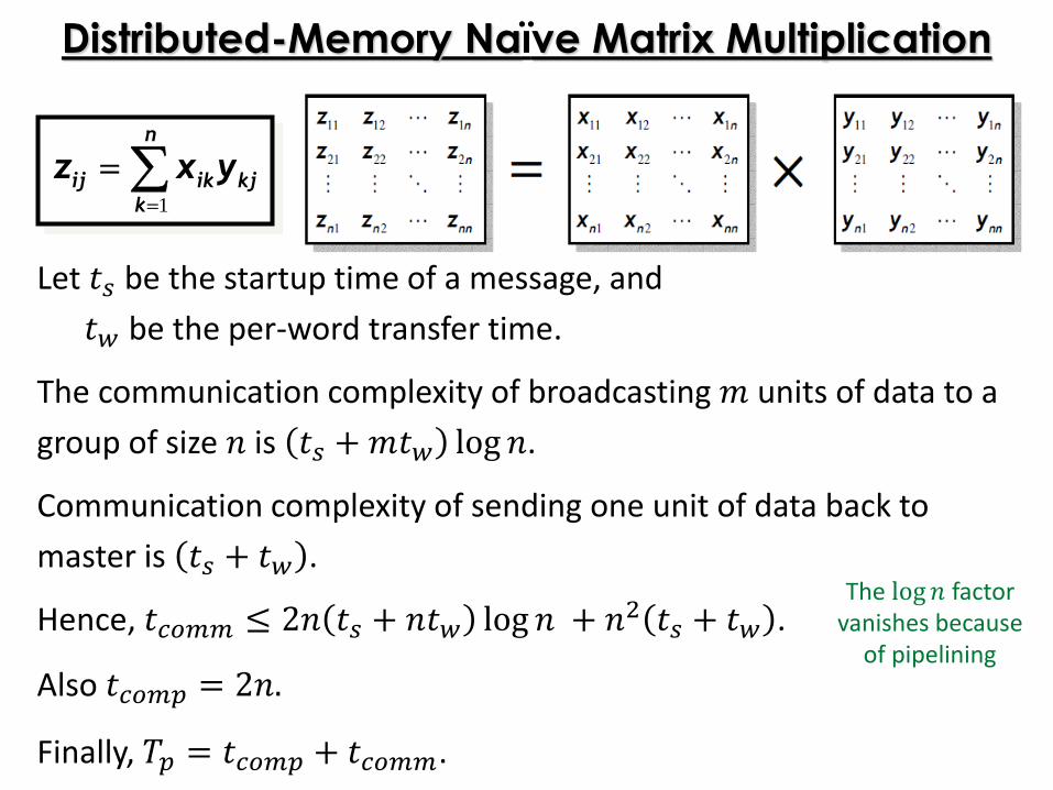
Let 𝑡𝑠 be the startup time of a message, and
𝑡𝑤 be the per-word transfer time.
The communication complexity of broadcasting 𝑚 units of data to a
group of size 𝑛 is 𝑡𝑠 +𝑚𝑡𝑤 log 𝑛.
Communication complexity of sending one unit of data back to
master is 𝑡𝑠 + 𝑡𝑤 .
Hence, 𝑡𝑐𝑜𝑚𝑚 ≤ 2𝑛 𝑡𝑠 + 𝑛𝑡𝑤 log 𝑛 + 𝑛2 𝑡𝑠 + 𝑡𝑤 .
Also 𝑡𝑐𝑜𝑚𝑝 = 2𝑛.
Finally, 𝑇𝑝 = 𝑡𝑐𝑜𝑚𝑝 + 𝑡𝑐𝑜𝑚𝑚.
Distributed-Memory Naïve Matrix Multiplication
The log 𝑛 factor vanishes because
of pipelining
Scaling Laws
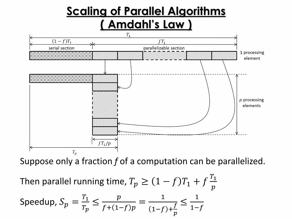
Scaling of Parallel Algorithms( Amdahl’s Law )
Suppose only a fraction f of a computation can be parallelized.
Then parallel running time, 𝑇𝑝 ≥ 1 − 𝑓 𝑇1 + 𝑓𝑇1
𝑝
Speedup, 𝑆𝑝 =𝑇1
𝑇𝑝≤
𝑝
𝑓+ 1−𝑓 𝑝=
1
1−𝑓 +𝑓
𝑝
≤1
1−𝑓
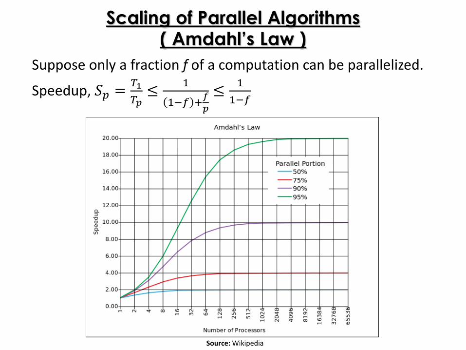
Scaling of Parallel Algorithms( Amdahl’s Law )
Suppose only a fraction f of a computation can be parallelized.
Speedup, 𝑆𝑝 =𝑇1
𝑇𝑝≤
1
1−𝑓 +𝑓
𝑝
≤1
1−𝑓
Source: Wikipedia
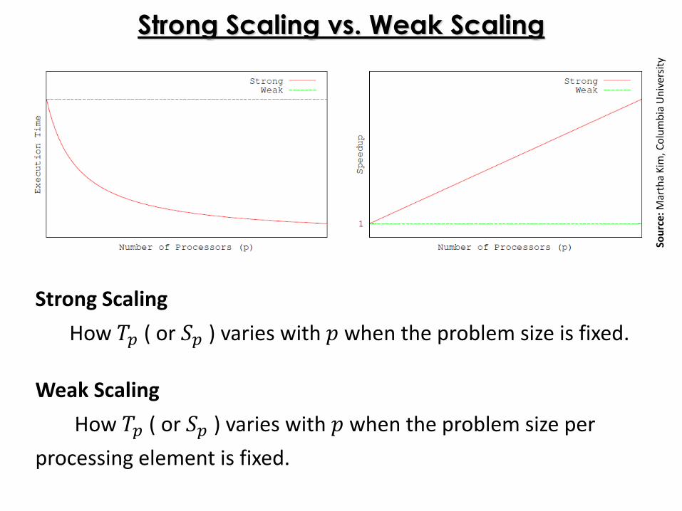
Strong Scaling
How 𝑇𝑝 ( or 𝑆𝑝 ) varies with 𝑝 when the problem size is fixed.
Strong Scaling vs. Weak Scaling
Weak Scaling
How 𝑇𝑝 ( or 𝑆𝑝 ) varies with 𝑝 when the problem size per
processing element is fixed.
Sou
rce:
Mar
tha
Kim
, Co
lum
bia
Un
iver
sity
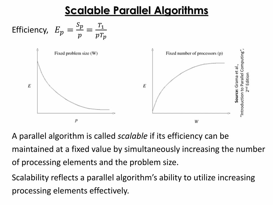
A parallel algorithm is called scalable if its efficiency can be
maintained at a fixed value by simultaneously increasing the number
of processing elements and the problem size.
Scalability reflects a parallel algorithm’s ability to utilize increasing
processing elements effectively.
Scalable Parallel Algorithms
Efficiency, 𝐸𝑝 =𝑆𝑝
𝑝=
𝑇1
𝑝𝑇𝑝
Sou
rce:
Gra
ma
et a
l.,
“In
tro
du
ctio
n t
o P
aral
lel C
om
pu
tin
g”,
2n
dEd
itio
n

“We used to joke that
“parallel computing is the future, and always will be,”
but the pessimists have been proven wrong.”
— Tony Hey
Now Have Fun!