General High-order Rogue Waves of the (1+1)-DimensionalYajima–Oikawa System

Junchao Chen1,2, Yong Chen2+, Bao-Feng Feng3†, Ken-ichi Maruno4‡, and Yasuhiro Ohta5§

1Department of Mathematics, Lishui University, Lishui, 323000, People’s Republic of China2Shanghai Key Laboratory of Trustworthy Computing, East China Normal University,

Shanghai, 200062, People’s Republic of China3School of Mathematical and Statistical Sciences, The University of Texas Rio Grande Valley, Edinburg, TX 78539, U.S.A.

4Department of Applied Mathematics, School of Fundamental Science and Engineering, Faculty of Science and Engineering,Waseda University, Shinjuku, Tokyo 169-8555, Japan

5Department of Mathematics, Kobe University, Kobe 657-8501, Japan

(Received April 10, 2018; revised June 24, 2018; accepted June 27, 2018; published online August 17, 2018)

General high-order rogue wave solutions for the (1+1)-dimensional Yajima–Oikawa (YO) system are derived byusing the Hirota’s bilinear method and the KP hierarchy reduction method. These rogue wave solutions are presented interms of determinants in which the elements are algebraic expressions. The dynamics of first-order and higher-orderrogue wave are investigated in details for different values of the free parameters. It is shown that the fundamental (first-order) rogue waves can be classified into three different patterns: bright, intermediate and dark ones. The higher-orderrogue waves correspond to the superposition of fundamental rogue waves. Especially, compared with the nonlinearSchrödinger equation, there exists an essential parameter α to control the pattern of rogue wave for both first-order andhigher-order rogue waves since the YO system does not possess the Galilean invariance.

1. Introduction

Rogue waves, which are initially used for the vividdescription of the spontaneous and monstrous ocean surfacewaves,1) have recently attracted considerable attention bothexperimentally and theoretically. Rogue waves have beenobserved in a variety of different fields, including opticalsystems,2–4) Bose–Einstein condensates,5,6) superfluids,7,8)

plasma,9,10) capillary waves11) and even finance.12) Comparedwith the stable solitons, rogue waves are the localizedstructures with the instability and unpredictability.13,14) Atypical model for characterizing the rogue wave is thecelebrated nonlinear Schrödinger (NLS) equation. The mostfundamental rogue wave of the NLS equation is described byPeregrine soliton,15) which is the first-order rogue wave andexpressed in a simple rational form including the polynomialsup to second order. This rational solution has localizedbehavior in both space and time, and its maximum amplitudeattains three times the constant background. The Peregrinesoliton can be obtained from a breather solution when theperiod is taken to infinity. More recently, significant progresson higher-order rogue waves has been made16–41) since a fewspecial higher-order rogue waves from first-order to fourth-order were provided theoretically by Akhmediev et al.16) viathe Darboux transformation. The higher-order rogue waveswere also excited experimentally in a water wave tank,42,43)

which guarantees that such nonlinear complicated waves aremeaningful physically. In fact, higher-order rogue waves canbe treated as the nonlinear superposition of fundamentalrogue wave and they are usually expressed in terms ofcomplicated higher-order rational polynomials. These higher-order waves were also localized in both coordinates andcould exhibit higher peak amplitudes or multiple intensitypeaks.

Another major development of importance is the study ofrogue waves in multicomponent coupled systems, as a lot ofcomplex physical systems usually contain interacting wavecomponents with different modes and frequencies.44–59) As

stated in Ref. 44, the cross-phase modulation term in coupledsystems leads to the varying instability regime characters.Due to the additional degrees of freedom, there exist moreabundant pattern structures and dynamics characters forrogue waves in coupled systems. For instance, in the scalarNLS equation, because of the existence of Galileaninvariance, the velocity of the background field does notinfluence the pattern of rogue waves. However, for thecoupled NLS system, the relative velocity between differentcomponent fields has real physical effects, and cannot beremoved by any trivial transformation. This fact brings somenovel patterns for rogue waves such as dark rogue waves,45)

the interaction between rogue waves and other nonlinearwaves,45,46) a four-petaled flower structure47) and so on.In particular, those more various higher-order rogue wavesin coupled nonlinear models enrich the realization andunderstanding of the mechanisms underlying the complexdynamics of rogue waves.

Among coupled wave dynamics systems, the long wave-short wave resonance interaction (LSRI) is a fascinatingphysical process in which a resonant interaction takes placebetween a weakly dispersive long-wave (LW) and a short-wave (SW) packet when the phase velocity of the formerexactly or almost matches the group velocity of thelatter.60,61) The theoretical investigation of this LSRI wasfirst done by Zakharov62) on Langmuir waves in plasma. Inthe case of long wave propagating in one direction, thegeneral Zakharov system was reduced to the LSRI systemwhich is often called the one-dimensional (1D) Yajima–Oikawa (YO) system.63) This phenomenon has beenpredicted in diverse areas such as plasma physics,62,63)

hydrodynamics64–68) and nonlinear optics.69,70) For instance,this resonance interaction can occur between the long gravitywave and the capillary-gravity one,64) between long and shortinternal waves,65) and between a long internal wave and ashort surface wave in a two layer fluid.66) In a second-ordernonlinear negative refractive index medium, it can beachieved when the short wave lies on the negative index

Journal of the Physical Society of Japan 87, 094007 (2018)

https://doi.org/10.7566/JPSJ.87.094007

094007-1 ©2018 The Physical Society of Japan

J. Phys. Soc. Jpn.Downloaded from journals.jps.jp by 24.243.110.153 on 08/17/18

branch while the long wave resides in the positive indexbranch.70) The 1D YO system (1D LSRI system) can bewritten in a dimensionless form:

iSt � Sxx þ SL ¼ 0; ð1ÞLt ¼ �4ðjSj2Þx; ð2Þ

where S and L represent the short wave and long wavecomponent, respectively. The 1D YO system was shown to beintegrable with a Lax pair, and was solved by the inversescattering transform method.63) It admits both bright anddark soliton solutions.67,68) In Refs. 71 and 72, it is shownthat the 1D YO system can be derived from the so-calledk-constrained KP hierarchy with k ¼ 2 while the NLSequation with k ¼ 1. Very recently, the first-order roguewave solutions to the 1D YO system have been derived byusing the Hirota’s bilinear method73) and the Darbouxtransformation.74,75) These vector parametric solutions indi-cate interesting structures such that the long wave field alwayskeeps a single hump structure, whereas the short-wave fieldcan be manifested as bright, intermediate and dark roguewave. In our previous paper,30) rational solutions includinglump solutions and rogue wave solutions of the 2D multi-component YO system were presented and some rogue wavesolutions of the 1D multi-component YO system throughreduction were discussed. Nevertheless, as far as we know,there is no report about high-order rogue wave solutions forthe 1D YO system. Therefore, the objective of present paper isto study high-order rogue wave solutions of the 1D YOsystem (1)–(2) by using the bilinear method in the frameworkof KP hierarchy reduction. As will be shown in the subsequentsection, a general rogue wave solutions in the form of Gramdeterminant is derived based on Hirota’s bilinear method andthe KP hierarchy reduction method. This determinant solutioncan generate rogue waves of any order without singularity.

The remainder of this paper is organized as follows. InSect. 2, we start with a set of bilinear equations satisfied bythe τ functions in Gram determinant of the KP hierarchy, andreduce them to bilinear equations satisfied by the 1D YOsystem (1)–(2). The reductions include mainly dimensionreduction and complex conjugate reduction. We shouldemphasize here that the most crucial and difficult issue isto find a general algebraic expression for the element ofdeterminant such that the dimension reduction can berealized. In Sect. 3, the dynamical behaviors of fundamentaland higher-order rogue wave solutions are illustrated fordifferent choices of free parameters. The paper is concludedin Sect. 4 by a brief summary and discussion.

2. Derivation of General Rogue Wave Solutions

This section is the core of the present paper, in which anexplicit expression for general rogue wave solutions of the1D YO system (1)–(2) will be derived by Hirota’s bilinearmethod. To this end, let us first introduce dependent variabletransformations

S ¼ ei½�xþðhþ�2Þt� g

f; L ¼ h � 2

@2

@x2log f; ð3Þ

where f is a real-valued function, g is a complex-valuedfunction and α and h are real constants. Then the 1D YOsystem (1)–(2) is converted into the following bilinearequations

ðD2x þ 2i�Dx � iDtÞg � f ¼ 0; ð4Þ

ðDxDt þ 4Þ f � f ¼ 4gg�; ð5Þwhere � denotes the complex conjugation hereafter and the Dis Hirota’s bilinear differential operator defined by

DnxD

mt ða � bÞ

¼ @

@x� @

@x0

� �n @

@t� @

@t0

� �maðx; tÞbðx0; t0Þjx¼x0;t¼t0 :

Prior to the tedious process in deriving the polynomialsolutions of the functions f and g, we highlight the main stepsof the detailed derivation, as shown in the subsequentsubsections.

Firstly, we start from the following bilinear equations ofthe KP hierarchy:

ðD2x1þ 2aDx1 � Dx2 Þ�nþ1 � �n ¼ 0; ð6Þ

1

2Dx1Dta � 1

� ��n � �n ¼ ��nþ1�n�1; ð7Þ

which admit a wide class of solutions in terms of Gram orWronski determinant. Among these determinant solutions,we need to look for algebraic solutions to satisfy thereduction condition:

ð@x2 þ 2i@ta Þ�n ¼ c�n; ð8Þsuch that these algebraic solutions satisfy the (1+1)-dimen-sional bilinear equations:

ðD2x1þ 2aDx1 � Dx2 Þ�nþ1 � �n ¼ 0; ð9Þ

ðiDx1Dx2 � 4Þ�n � �n ¼ �4�nþ1�n�1: ð10ÞFurthermore, by introducing the variable transformations:

x1 ¼ x; x2 ¼ �it; ð11Þand taking f ¼ �0, g ¼ �1, h ¼ ��1, and a ¼ i�, the abovebilinear equations (9)–(10) become

ðD2x þ 2i�Dx � iDtÞg � f ¼ 0; ð12Þ

ðDxDt þ 4Þ f � f ¼ 4gh: ð13ÞLastly, by requiring the real and complex conjugationcondition:

f ¼ �0 : real; g ¼ �1; h ¼ ��1 ¼ g�; ð14Þin the algebraic solutions, then the bilinear equations (12)–(13) are reduced to the bilinear equations (4)–(5), hence thegeneral higher-order rogue wave solutions are obtainedthrough the reductions.

2.1 Gram determinant solution for the bilinear equations inthe KP hierarchy

In this subsection, through the Lemma below, we presentand prove that a pair of bilinear equations are satisfied by theτ functions of the KP hierarchy.

Lemma 2.1. Let mðnÞij , depending on ’ðnÞ

i and ðnÞj , be

function of the variables x1, x2, and ta, and satisfy thefollowing differential and difference relations:

@x1mðnÞij ¼ ’ðnÞ

i ðnÞj ;

@x2mðnÞij ¼ ½@x1’ðnÞ

i � ðnÞj � ’ðnÞ

i ½@x1 ðnÞj �;

@tamðnÞij ¼ �’ðn�1Þ

i ðnþ1Þj ;

J. Phys. Soc. Jpn. 87, 094007 (2018) J. Chen et al.

094007-2 ©2018 The Physical Society of Japan

J. Phys. Soc. Jpn.Downloaded from journals.jps.jp by 24.243.110.153 on 08/17/18

mðnþ1Þij ¼ mðnÞ

ij þ ’ðnÞi ðnþ1Þ

j ; ð15Þwhere ’ðnÞ

i and ðnÞj are functions satisfying

@x2’ðnÞi ¼ @2x1’

ðnÞi ; ’ðnþ1Þ

i ¼ ð@x1 � aÞ’ðnÞi ;

@x2 ðnÞj ¼ �@2x1 ðnÞ

j ; ðn�1Þi ¼ �ð@x1 þ aÞ ðnÞ

j : ð16ÞThen the � functions of the following determinant form

�n ¼ det1�i; j�N

ðmðnÞij Þ; ð17Þ

satisfy the following bilinear equations (6) and (7) in KPhierarchy:

ðD2x1þ 2aDx1 �Dx2Þ�nþ1 � �n ¼ 0; ð18Þ

1

2Dx1Dta � 1

� ��n � �n ¼ ��nþ1�n�1: ð19Þ

Proof. By using the differential formula of determinant

@x det1�i; j�N

ðaijÞ ¼XNi;j¼1

�ij@xaij; ð20Þ

and the expansion formula of bordered determinant

detaij bi

cj d

!¼ �

XNi;j

�ijbicj þ d detðaijÞ; ð21Þ

with �ij being the ði; jÞ-cofactor of the matrix (aij), one cancheck that the derivatives and shifts of the τ function areexpressed by the bordered determinants as follows:

@x1�n ¼mðnÞij ’ðnÞ

i

� ðnÞj 0

����������; @2x1�n ¼

mðnÞij @x1’

ðnÞi

� ðnÞj 0

���������� þ

mðnÞij ’ðnÞ

i

�@x1 ðnÞj 0

����������;

@x2�n ¼mðnÞij @x1’

ðnÞi

� ðnÞj 0

���������� �

mðnÞij ’ðnÞ

i

�@x1 ðnÞj 0

����������; @ta�n ¼

mðnÞij ’ðn�1Þ

i

ðnþ1Þj 0

����������;

ð@x1@ta � 1Þ�n ¼mðnÞij ’ðn�1Þ

i ’ðnÞi

ðnþ1Þj 0 �1

� ðnÞj �1 0

��������

��������;

�nþ1 ¼mðnÞij ’ðnÞ

i

� ðnþ1Þj 1

����������; �n�1 ¼

mðnÞij ’ðn�1Þ

i

ðnÞj 1

����������; ð@x1 þ aÞ�nþ1 ¼

mðnÞij @x1’

ðnÞi

� ðnþ1Þj a

����������;

ð@x1 þ aÞ2�nþ1 ¼mðnÞij @2x1’

ðnÞi

� ðnþ1Þj a2

���������� þ

mðnÞij @x1’

ðnÞi ’ðnÞ

i

� ðnþ1Þj a 1

� ðnÞj 0 0

��������

��������;

ð@x2 þ a2Þ�nþ1 ¼mðnÞij @2x1’

ðnÞi

� ðnþ1Þj a2

���������� �

mðnÞij @x1’

ðnÞi ’ðnÞ

i

� ðnþ1Þj a 1

� ðnÞj 0 0

��������

��������:With the help of these relations, one has

ð@x1@ta � 1Þ�n � �n � @x1�n � @ta�n þ ð��n�1Þð��nþ1Þ

¼mðnÞij ’ðn�1Þ

i ’ðnÞi

ðnþ1Þj 0 �1

� ðnÞj �1 0

��������

�������� � jmðnÞij j �

mðnÞij ’ðnÞ

i

� ðnÞj 0

���������� �

mðnÞij ’ðn�1Þ

i

ðnþ1Þj 0

����������

þmðnÞij ’ðn�1Þ

i

� ðnÞj �1

���������� �

mðnÞij ’ðnÞ

i

ðnþ1Þj �1

����������; ð22Þ

1

2ð@2x1 þ 2a@x1 � @x2 Þ�nþ1 � �n � ð@x1 þ aÞ�nþ1 � @x1�n þ �nþ1 � 1

2ð@2x1 þ @x2 Þ�n

¼mðnÞij @x1’

ðnÞi ’ðnÞ

i

� ðnþ1Þj a 1

� ðnÞj 0 0

��������

�������� � jmðnÞij j �

mðnÞij ’ðnÞ

i

� ðnÞj 0

���������� �

mðnÞij @x1’

ðnÞi

� ðnþ1Þj a

����������

þmðnÞij @x1’

ðnÞi

� ðnÞj 0

���������� �

mðnÞij ’ðnÞ

i

� ðnþ1Þj 1

����������: ð23Þ

The r.h.s of both (22) and (23) are identically zero because of the Jacobi identity and hence the τ functions (17) satisfy thebilinear equations (18) and (19). This completes the proof. □

J. Phys. Soc. Jpn. 87, 094007 (2018) J. Chen et al.

094007-3 ©2018 The Physical Society of Japan

J. Phys. Soc. Jpn.Downloaded from journals.jps.jp by 24.243.110.153 on 08/17/18

2.2 Algebraic solutions for the (1+1)-dimensional YOsystem

This subsection is crucial in the KP hierarchy reductionmethod. We will construct an algebraic expression for theelements of τ function of preceding subsection so that thedimension reduction condition (8) is satisfied. The mainresult is given by the following Lemma.

Lemma 2.2. Suppose the entries mð��nÞkl of the matrix m

are

mð��nÞkl ¼ ðAð�Þ

k Bð�Þl mðnÞÞjp¼�;q¼�� ; ð24Þ

where

mðnÞ ¼ 1

p þ q� p � a

q þ a

� �ne�þ�; � ¼ px1 þ p2x2;

� ¼ qx1 � q2x2;

� ¼ �r þ i�i; �r ¼ �ffiffiffi3

p

12

K2 � 4�2

K;

�i ¼ 1

12K þ 1

3

�2

Kþ 2

3�;

K ¼ ð8�3 þ 108 þ 12ffiffiffiffiffiffiffiffiffiffiffiffiffiffiffiffiffiffiffiffiffi12�3 þ 81

pÞ1=3; � > � 3

221=3

� �;

and Að�Þk and Bð�Þ

l are differential operators with respect to pand q, respectively, given by

Að�Þn ¼

Xnk¼0

að�Þk½ðp � aÞ@p�n�k

ðn � kÞ! ; n 0; ð25Þ

Bð�Þn ¼

Xnk¼0

bð�Þk½ðq þ aÞ@q�n�k

ðn � kÞ! ; n 0; ð26Þ

where að�Þk and bð�Þk are constants satisfying the iteratedrelations

að�þ1Þk ¼Xkj¼0

2 jþ2ðp � aÞ2 þ ð�1Þ j 2i

p � aþ 2aðp � aÞ

ð j þ 2Þ! að�Þk�j;

� ¼ 0; 1; 2; . . . ; ð27Þ

bð�þ1Þk ¼Xkj¼0

2 jþ2ðq þ aÞ2 � ð�1Þ j 2i

q þ a� 2aðq þ aÞ

ð j þ 2Þ! bð�Þk�j;

� ¼ 0; 1; 2; . . . ; ð28Þthen the determinant

�n ¼ det1�i; j�N

ðmðN�i;N�j;nÞ2i�1;2j�1 Þ

¼

mðN�1;N�1;nÞ11 mðN�1;N�2;nÞ

13 � � � mðN�1;0;nÞ1;2N�1

mðN�2;N�1;nÞ31 mðN�2;N�2;nÞ

33 � � � mðN�2;0;nÞ3;2N�1

..

. ... ..

.

mð0;N�1;nÞ2N�1;1 mð0;N�2;nÞ

2N�1;3 � � � mð0;0;nÞ2N�1;2N�1

������������

������������; ð29Þ

satisfies the bilinear equationsðD2

x1þ 2aDx1 � Dx2 Þ�nþ1 � �n ¼ 0; ð30Þ

ðiDx1Dx2 � 4Þ�n � �n ¼ �4�nþ1�n�1: ð31Þ

Proof. Firstly, we introduce the functions ~mðnÞ, ~’ðnÞ, and~ ðnÞ of the form

~mðnÞ ¼ 1

p þ q� p � a

q þ a

� �ne~�þ ~�; ~’ðnÞ ¼ ðp � aÞne ~�;

~ ðnÞ ¼ � 1

q þ a

� �ne ~�;

where

~� ¼ 1

p � ata þ px1 þ p2x2; ~� ¼ 1

q þ ata þ qx1 � q2x2:

These functions satisfy the differential and difference rules:

@x1 ~mðnÞ ¼ ~’ðnÞ ~ ðnÞ;

@x2 ~mðnÞ ¼ ½@x1 ~’ðnÞ� ~ ðnÞ � ~’ðnÞ½@x1 ~ ðnÞ�;

@ta ~mðnÞ ¼ � ~’ðn�1Þ ~ ðnþ1Þ;

~mðnþ1Þ ¼ ~mðnÞ þ ~’ðnÞ ~ ðnþ1Þ;and

@x2 ~’ðnÞ ¼ @2x1 ~’

ðnÞ; ~’ðnþ1Þ ¼ ð@x1 � aÞ ~’ðnÞ;

@x2 ~ ðnÞ ¼ �@2x1 ~ ðnÞ; ~ ðn�1Þ ¼ �ð@x1 þ aÞ ~ ðnÞ:

We then define~mð��nÞij ¼ Að�Þ

i Bð�Þj ~mðnÞ; ~’ð�nÞ

i ¼ Að�Þi ~’ðnÞ;

~ ð�nÞj ¼ Bð�Þ

j ~ ðnÞ: ð32ÞSince the operators Að�Þ

i and Bð�Þj commute with differential

operators @x1 , @x2 , and @ta , these functions ~mð��nÞij , ~’ð�nÞ

i , and~ ð�nÞj obey the differential and difference relations as well

(15)–(16). From Lemma 2.1, we know that for an arbitrarysequence of indices ði1; i2; . . . ; iN; �1; �2; . . . ; �N; j1; j2; . . . ;jN; �1; �2; . . . ; �NÞ, the determinant

~�n ¼ det1�k;l�N

ð ~mð�k;�l;nÞik; jl

Þsatisfies the bilinear equations (18) and (19), for instance,the bilinear equations (18) and (19) hold for ~�n ¼det1�i; j�Nð ~mðN�i;N�j;nÞ

2i�1;2j�1 Þ with arbitrary parameters p and q.Based on the Leibniz rule, one has,

½ðp � aÞ@p�m p2 þ 2i

p � a

� �

¼Xml¼0

m

l

!2lðp � aÞ2 þ ð�1Þl 2i

p � aþ 2aðp � aÞ

� �

� ½ðp � aÞ@p�m�l þ a2½ðp � aÞ@p�m; ð33Þand

½ðq þ aÞ@q�m q2 � 2i

q þ a

� �

¼Xml¼0

m

l

!2lðq þ aÞ2 � ð�1Þl 2i

q þ a� 2aðq þ aÞ

� �

� ½ðq þ aÞ@q�m�l þ a2½ðq þ aÞ@q�m: ð34ÞFurthermore, one can derive

Að�Þn ; p2 þ 2i

p � a

� �

¼Xn�1k¼0

að�Þkðn � kÞ! ððp � aÞ@pÞn�k; p2 þ 2i

p � a

� �

¼Xn�1k¼0

að�Þkðn � kÞ!

Xn�kl¼1

n � k

l

!

J. Phys. Soc. Jpn. 87, 094007 (2018) J. Chen et al.

094007-4 ©2018 The Physical Society of Japan

J. Phys. Soc. Jpn.Downloaded from journals.jps.jp by 24.243.110.153 on 08/17/18

� 2lðp � aÞ2 þ ð�1Þl 2i

p � aþ 2aðp � aÞ

� �� ððp � aÞ@pÞn�k�l;

where ½; � is the commutator defined by ½X; Y� ¼ XY � YX.Let ζ be the solution of the cubic equation

2ðp � aÞ2 � 2i

p � aþ 2aðp � aÞ ¼ 0;

with a ¼ i�, then ζ has an explicit expression givenpreviously. Hence we have

Að�Þn ; p2 þ 2i

p � a

� �����p¼�

¼ 0;

for n ¼ 0; 1 and

Að�Þn ; p2 þ 2i

p � a

� �����p¼�

¼Xn�2k¼0

að�Þkðn � kÞ!

Xn�kl¼2

n � k

l

!2lðp � aÞ2 þ ð�1Þl 2i

p � aþ 2aðp � aÞ

� ½ðp � aÞ@p�n�k�ljp¼�

¼Xn�2k¼0

Xn�k�2j¼0

að�Þkð j þ 2Þ!ðn � k � j � 2Þ! 2 jþ2ðp � aÞ2 þ ð�1Þ j 2i

p � aþ 2aðp � aÞ

�

� ½ðp � aÞ@p�n�k�j�2jp¼�

¼Xn�2k̂¼0

Xk̂|̂¼0

2 |̂þ2ðp � aÞ2 þ ð�1Þ |̂ 2i

p � aþ 2aðp � aÞ

ð |̂ þ 2Þ! að�Þk̂�|̂

0BBB@

1CCCA ððp � aÞ@pÞn�2�k̂

ðn � 2 � k̂Þ!

�����p¼�

¼Xn�2k̂¼0

að�þ1Þk̂

ððp � aÞ@pÞn�2�k̂ðn � 2 � k̂Þ!

�����p¼�

¼ Að�þ1Þn�2 jp¼�;

for n 2. Thus the differential operator Að�Þn satisfies the following relation

Að�Þn ; p2 þ 2i

p � a

� �����p¼�

¼ Að�þ1Þn�2 jp¼�; ð35Þ

where we define Að�Þn ¼ 0 for n < 0.

Similarly, it is shown that the differential operator Bð�Þn satisfies

Bð�Þn ; q2 � 2i

q þ a

� �����q¼��

¼ Bð�þ1Þn�2 jq¼�� ; ð36Þ

where we define Bð�Þn ¼ 0 for n < 0.

Consequently, by referring to above two relations, we have

ð@x2 þ 2i@ta Þ ~mð��nÞkl jp¼�;q¼��

¼ ½Að�Þk Bð�Þ

l ð@x2 þ 2i@taÞ ~mðnÞ�jp¼�;q¼��

¼ Að�Þk Bð�Þ

l p2 � q2 þ 2i1

p � aþ 1

q þ a

� �� �~mðnÞ

� �����p¼�;q¼��

¼ Að�Þk p2 þ 2i

p � a

� �Bð�Þl ~mðnÞ

� �����p¼�;q¼��

� Að�Þk Bð�Þ

l q2 � 2i

q þ a

� �~mðnÞ

� �����p¼�;q¼��

¼ p2 þ 2i

p � a

� �Að�Þk þ Að�þ1Þ

k�2

� �Bð�Þl ~mðnÞ

� ����p¼�;q¼��

� Að�Þk q2 � 2i

q þ a

� �Bð�Þl þ Bð�þ1Þ

l�2

� �~mðnÞ

� ����p¼�;q¼��

¼ �2 þ 2i

� � i�

� �~mð��nÞkl jp¼�;q¼�� þ ~mð�þ1;�;nÞ

k�2;l jp¼�;q¼��

� ��2 � 2i

�� þ i�

� �~mð��nÞkl jp¼�;q¼�� � ~mð�;�þ1;nÞ

k;l�2 jp¼�;q¼�� :

By using the formula (20) and the above relation, the differential of the following determinant

J. Phys. Soc. Jpn. 87, 094007 (2018) J. Chen et al.

094007-5 ©2018 The Physical Society of Japan

J. Phys. Soc. Jpn.Downloaded from journals.jps.jp by 24.243.110.153 on 08/17/18

~~�n ¼ det1�i; j�N

ð ~mðN�i;N�j;nÞ2i�1;2j�1 jp¼�;q¼�� Þ

can be calculated as

ð@x2 þ 2i@ta Þ~~�n

¼XNi¼1

XNj¼1

�ijð@x2 þ 2i@ta Þð ~mðN�i;N�j;nÞ2i�1;2j�1 jp¼�;q¼�� Þ

¼XNi¼1

XNj¼1

�ij

"�2 þ 2i

� � i�

� �~mðN�i;N�j;nÞ2i�1;2j�1 jp¼�;q¼�� þmðN�iþ1;N�j;nÞ

2i�3;2j�1 jp¼�;q¼��

� ��2 � 2i

�� þ i�

� �~mðN�i;N�j;nÞ2i�1;2j�1 jp¼�;q¼�� � mðN�i;N�jþ1;nÞ

2i�1;2j�3 jp¼�;q¼��#

¼ �2 þ 2i

� � i�

� �N~~�n þ

XNi¼1

XNj¼1

�ij ~mðN�iþ1;N�j;nÞ2i�3;2j�1 jp¼�;q¼��

� ��2 � 2i

�� þ i�

� �N~~�n �

XNi¼1

XNj¼1

�ij ~mðN�i;N�jþ1;nÞ2i�1;2j�3 jp¼�;q¼�� ;

where �ij is the ði; jÞ-cofactor of the matrix

ð ~mðN�i;N�j;nÞ2i�1;2j�1 jp¼�;q¼�� Þ1�i; j�N. For the termPNi¼1PN

j¼1 �ij ~mðN�iþ1;N�j;nÞ2i�3;2j�1 jp¼�;q¼�� , it vanishes, since for

i ¼ 1 this summation is a determinant with the elements infirst row being zero and for i ¼ 2; 3; . . . this summation isa determinant with two identical rows. Similarly, the termPN

i¼1PN

j¼1 �ij ~mðN�i;N�jþ1;nÞ2i�1;2j�3 jp¼�;q¼�� vanishes. Therefore, ~~�n

satisfies the reduction condition

ð@x2 þ 2i@taÞ~~�n ¼ �2 � ��2 þ 2i

� � i�þ 2i

�� þ i�

� �N~~�n: ð37Þ

Since ~~�n is a special case of ~�n, it also satisfies the bilinearequations (18) and (19) with �n replaced by ~~�n. From (18),(19), and (37), it is obvious that ~~�n satisfies the (1+1)-dimensional bilinear equations

ðD2x1þ 2aDx1 � Dx2 Þ~~�nþ1 � ~~�n ¼ 0; ð38Þ

ðiDx1Dx2 � 4Þ~~�n � ~~�n ¼ �4~~�nþ1~~�n�1: ð39ÞDue to the reduction condition (37), ta becomes a dummyvariable which can be taken as zero. Thus ~mðN�i;N�j;nÞ

2i�1;2j�1 jp¼�;q¼��and ~~�n reduce to mðN�i;N�j;nÞ

2i�1;2j�1 and �n (29) in Lemma 2.2.Therefore �n satisfies the bilinear equations (30) and (31) andthe proof is complete. □

2.3 Complex conjugate condition and regularityFrom Lemma 2.2, by taking the independent variable

transformations:

x1 ¼ x; x2 ¼ �it; ð40Þit is found that f ¼ �0, g ¼ �1 and h ¼ ��1 satisfy the (1+1)-dimensional bilinear equations:

ðD2x þ 2i�Dx � iDtÞg � f ¼ 0; ð41Þ

ðDxDt þ 4Þ f � f ¼ 4gh: ð42ÞNext we consider the complex conjugate condition and theregularity (non-singularity) of solutions. The complexconjugate condition requires

�0 : real; ��1 ¼ ��1: ð43Þ

Since x1 ¼ x is real and x2 ¼ �it is pure imaginary, thecomplex conjugate condition can be easily satisfied by takingthe parameters að0Þk and bð0Þk to be complex conjugate to eachother. It then follows

bð�Þk jq¼�� ¼ ðað�Þk jp¼�Þ�; ð44Þfor � ¼ 0; 1; 2; . . .. Then, by referring to (44), we have

mð�;�;nÞ�ij ¼ mð�;�;nÞ

ij jað�Þk$bð�Þ

k;x2$�x2;a$�a;�$�� ¼ mð�;�;�nÞ

ji ; ð45Þwhich implies

��n ¼ ��n: ð46ÞOn the other hand, under the condition (44), we can showthat �0 is nonzero for all ðx; tÞ. Note that f ¼ �0 is thedeterminant of a Hermitian matrix M ¼ ðmðN�i;N�j;0Þ

2i�1;2j�1 Þ1�i; j�N.From the appendix in Ref. 56, it is known that when the realpart of the parameter ζ is positive, the element of theHermitian matrix M can be written as an integral

mðN�i;N�j;0Þ2i�1;2j�1 ¼

Z x

�1AðN�iÞ2i�1 B

ðN�jÞ2j�1 e

�þ� dxjp¼�;q¼�� : ð47Þ

For any non-zero column vector ¼ ðv1; v2; . . . ; vNÞT and y

being its complex transpose, one can obtain

yM ¼XNi;j¼1

yi mðN�i;N�j;0Þ2i�1;2j�1 j

¼Z x

�1

XNi¼1

yi AðN�iÞ2i�1 e

�jp¼������

�����2

dx > 0;

which shows that the Hermitian matrix M is positive definite,hence the denominator f ¼ detM > 0.

When the real part of the parameter p is negative, theelement of the Hermitian matrix M can be cast into

mðN�i;N�j;0Þ2i�1;2j�1 ¼ �

Z þ1

x

AðN�iÞ2i�1 B

ðN�jÞ2j�1 e

�þ� dxjp¼�;q¼�� : ð48Þ

Then one obtains

yM ¼XNi;j¼1

yi mðN�i;N�j;0Þ2i�1;2j�1 j

J. Phys. Soc. Jpn. 87, 094007 (2018) J. Chen et al.

094007-6 ©2018 The Physical Society of Japan

J. Phys. Soc. Jpn.Downloaded from journals.jps.jp by 24.243.110.153 on 08/17/18

¼ �Z þ1

x

XNi¼1

yi AðN�iÞ2i�1 e

�jp¼������

�����2

dx < 0;

which proves that the Hermitian matrix M is negativedefinite, hence the denominator f ¼ detM < 0. Therefore, foreither positive or negative of the parameter ζ, the rogue wavesolution of the short wave and long wave components isalways nonsingular.

To summarize the results, we have the following theoremfor the general higher order rogue wave solutions of the 1DYO system (1)–(2):

Theorem 2.3. The 1D YO system (1)–(2) has the non-singular rational solutions

S ¼ ei½�xþðhþ�2Þt� �1

�0; L ¼ h � 2

@2

@x2log �0; ð49Þ

with

�n ¼ det1�i; j�N

ðmðN�i;N�j;nÞ2i�1;2j�1 Þ

¼

mðN�1;N�1;nÞ11 mðN�1;N�2;nÞ

13 � � � mðN�1;0;nÞ1;2N�1

mðN�2;N�1;nÞ31 mðN�2;N�2;nÞ

33 � � � mðN�2;0;nÞ3;2N�1

..

. ... ..

.

mð0;N�1;nÞ2N�1;1 mð0;N�2;nÞ

2N�1;3 � � � mð0;0;nÞ2N�1;2N�1

�����������

�����������; ð50Þ

where g ¼ �1, f ¼ �0, and h ¼ ��1, and the elements indeterminant �n are defined by

mð�;�;nÞi; j ¼

Xik¼0

Xjl¼0

að�Þkði � kÞ!

að�Þ�l

ð j � lÞ!� ½ðp � i�Þ@p�i�k½ðq þ i�Þ@q� j�l

� 1

p þ q� p � i�

q þ i�

� �neðpþqÞx�ðp

2�q2Þitjp¼�;q¼�� ; ð51Þand

� ¼ �r þ i�i; �r ¼ �ffiffiffi3

p

12

K2 � 4�2

K;

�i ¼ 1

12K þ 1

3

�2

Kþ 2

3�;

with

K ¼ ð8�3 þ 108 þ 12ffiffiffiffiffiffiffiffiffiffiffiffiffiffiffiffiffiffiffiffiffi12�3 þ 81

pÞ1=3; � > � 3

221=3

� �;

where að�Þk are complex constants and need to satisfy therelations:

að�þ1Þk ¼Xkj¼0

2 jþ2ðp � i�Þ2 þ ð�1Þ j 2i

p � i�þ 2i�ðp � i�Þ

ð j þ 2Þ!� að�Þk�j; � ¼ 0; 1; 2; . . . : ð52Þ

3. Dynamics of Rogue Wave Solutions

In this section, we analyze the dynamics of rogue wavesolutions to the 1D YO system in detail. To this end, wefix the parameter �r ¼

ffiffi3

p12

K2�4�2K without loss of generality.

Meanwhile, due to the fact that the long wave L is a real-valued function and its rogue wave structure is alwaysbright,73–75) in what follows, we omit the discussion of the

long wave component and only consider the dynamicalproperties of the complex short wave component S.3.1 Fundamental rogue wave

According to Theorem 2.3, in order to obtain the first-order rogue wave, we need to take N ¼ 1 in Eqs. (49)–(52).For simplicity, we set að0Þ0 ¼ bð0Þ0 ¼ 1, að0Þ1 ¼ bð0Þ1 ¼ 0, thenthe functions f and g take the form

f ¼ 1

�re2�rðxþ2�itÞð� þ 0Þ; ð53Þ

g ¼ 1

�re2�rðxþ2�itÞ � �r þ ið�i � �Þ

�r � ið�i � �Þ� �

� � 1

2þ 1

2i

� �� þ 1

2þ 1

2i

� �þ 0

� �; ð54Þ

with

¼ ðk1 þ ik2Þx þ ðh1 þ ih2Þt þ ðl1 þ il2Þ;

k1 ¼ 1

2ð� þ �r � �iÞ; k2 ¼ 1

2ð� � �r � �iÞ;

h1 ¼ �ð�i � �rÞ þ �2r þ 2�r�i � �2i ;

h2 ¼ �ð�i þ �rÞ þ �2r � 2�r�i � �2i ;

l1 ¼ �i � �

4�r� 1

4; l2 ¼ �i � �

4�rþ 1

4;

0 ¼ ð�i � �Þ28�2r

þ 1

8:

Thus, the fundamental rogue wave solution is given by

S ¼ e�i½�xþðhþ�2Þt� � �r þ ið�i � �Þ

�r � ið�i � �Þ� �

1 þ iðL1 þ L2Þ � 1=2

L21 þ L22 þ 0

� �;

ð55Þ

L ¼ h þ 4ðk1L1 þ k2L2Þ2 � ðk2L1 � k1L2Þ2 � ðk21 þ k22Þ0

ðL21 þ L22 þ 0Þ2;

ð56Þwhere L1 ¼ k1x þ h1t þ l1 and L2 ¼ k2x þ h2t þ l2.

It is found that the modular square of the short-wavecomponent jSj2 possesses critical points

ðx1; t1Þ ¼ 1

2�r; 0

� �; ð57Þ

ðx2; t2Þ ¼ 1

2

�1ð� � 2�iÞ�r�

þ 1

2�r;1

4

�1�r�

� �; ð58Þ

ðx3; t3Þ ¼ � 1

2

�2ð��i þ �2r � �2i Þ�2r�

þ 1

2�r;1

4

�2ð� � �iÞ�2r�

� �;

ð59Þwith

�1 ¼ �ffiffiffiffiffiffiffiffiffiffiffiffiffiffiffiffiffiffiffiffiffiffiffiffiffiffiffiffiffiffi3ð� � �iÞ2 � �2r

p;

�2 ¼ �ffiffiffiffiffiffiffiffiffiffiffiffiffiffiffiffiffiffiffiffiffiffiffiffiffiffiffiffiffiffi3�2r � ð� � �iÞ2

p;

� ¼ ð� � �iÞ2 þ �2r :

Note that ðx3; t3Þ are also two characteristic points, at whichthe values of the amplitude are zero.

At these points, the local quadratic forms are

Hð ~x; ~tÞ ¼ @2jSj2@x2

@2jSj2@t2

� @2jSj2@x@t

� �2" #�����

ð ~x;~t Þ;

J. Phys. Soc. Jpn. 87, 094007 (2018) J. Chen et al.

094007-7 ©2018 The Physical Society of Japan

J. Phys. Soc. Jpn.Downloaded from journals.jps.jp by 24.243.110.153 on 08/17/18

Hðx1; t1Þ ¼ � 16384�10r �21�

22

�4;

Hðx2; t2Þ ¼ 64�10r �21�

2

ð� � �iÞ10; Hðx3; t3Þ ¼ 64�22�

2; ð60Þ

and the second derivatives are

H1ð ~x; ~tÞ ¼ @2jSj2@x2

����ð ~x;~t Þ

;

H1ðx1; t1Þ ¼ 192�4r ½ð� � �iÞ2 � �2r ��2

;

H2ðx2; t2Þ ¼ � 6�4r�

ð� � �iÞ4; H3ðx3; t3Þ ¼ 6�: ð61Þ

Based on the above analysis, the fundamental rogue wavecan be classified into three patterns:

(a) Dark state (� 3221=3 < � ⩽ � 2

332=3): two local maxima

at ðx2; t2Þ with the jSj’s amplitudeffiffiffi�

p�i��, one local minimum

at ðx1; t1Þ with the jSj’s amplitude � �22

�. Especially, when

� ¼ � 2332=3, the local minimum is located at the character-

istic point ðx1; t1Þ ¼ ðx3; t3Þ ¼ ð1335=6; 0Þ.

(b) Intermediate state (� 2332=3 < � < 0): two local max-

ima at ðx2; t2Þ with the jSj’s amplitudeffiffiffi�

p�i��, two local minima

at two characteristic points ðx3; t3Þ.(c) Bright state (� ⩾ 0): two local minima at two

characteristic points ðx3; t3Þ, one local maxima at ðx1; t1Þwith the jSj’s amplitude �2

2

�. Particularly, � ¼ 0, the local

maximum is located at ðx1; t1Þ ¼ ðx2; t2Þ ¼ ð1331=2; 0Þ.

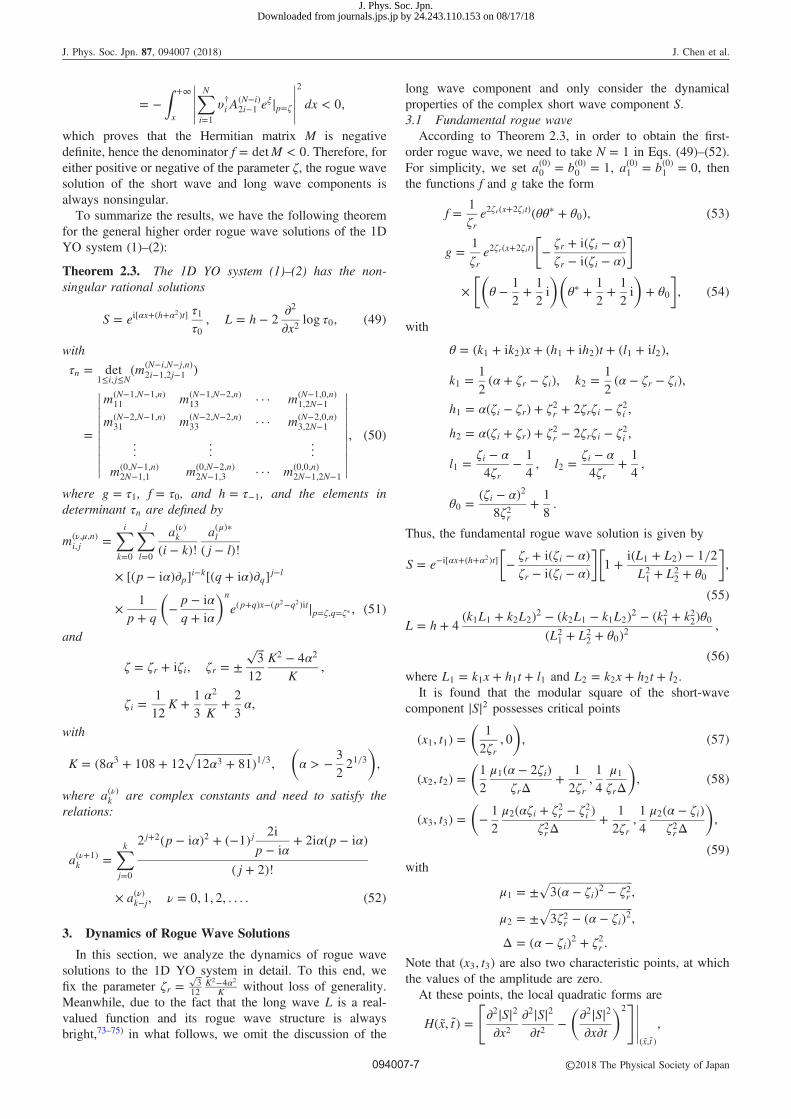
At the extreme points, the evolution of the amplitudes forthe short wave with the parameter α is exhibited in Fig. 1. Itcan be clearly seen that, for the dark state, as α changes from

� 3221=3 to � 2

332=3, the maximal amplitudes increase from 1

to 23

ffiffiffi3

pwhile the minimal one decreases from 1 to 0; for

the intermediate state, as α changes from � 2332=3 to 0, the

maximal amplitudes increase from (23

ffiffiffi3

pto 2 while the

minimal amplitude is always zero; for the bright state, as� 0, the maximal amplitude is changed from 2 to itsasymptotic value of 3 while the minimal value is alwayszero.

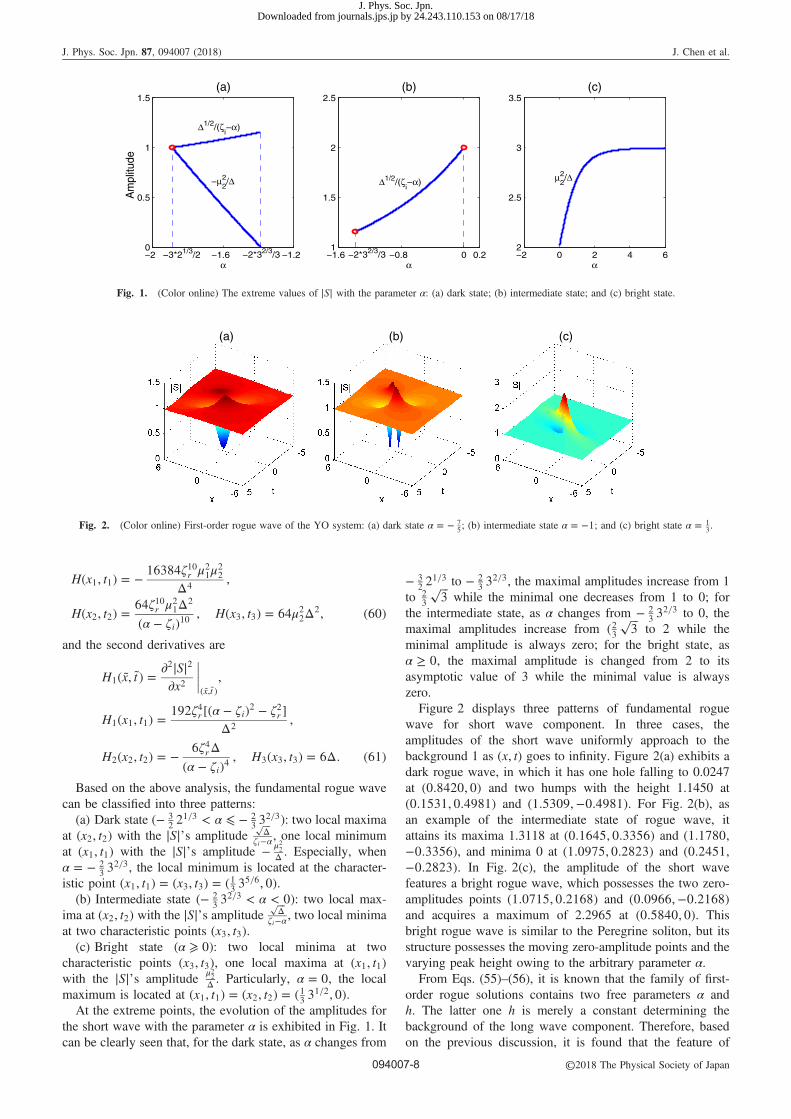
Figure 2 displays three patterns of fundamental roguewave for short wave component. In three cases, theamplitudes of the short wave uniformly approach to thebackground 1 as ðx; tÞ goes to infinity. Figure 2(a) exhibits adark rogue wave, in which it has one hole falling to 0.0247at ð0:8420; 0Þ and two humps with the height 1.1450 atð0:1531; 0:4981Þ and ð1:5309;�0:4981Þ. For Fig. 2(b), asan example of the intermediate state of rogue wave, itattains its maxima 1.3118 at ð0:1645; 0:3356Þ and ð1:1780;�0:3356Þ, and minima 0 at ð1:0975; 0:2823Þ and ð0:2451;�0:2823Þ. In Fig. 2(c), the amplitude of the short wavefeatures a bright rogue wave, which possesses the two zero-amplitudes points ð1:0715; 0:2168Þ and ð0:0966;�0:2168Þand acquires a maximum of 2.2965 at ð0:5840; 0Þ. Thisbright rogue wave is similar to the Peregrine soliton, but itsstructure possesses the moving zero-amplitude points and thevarying peak height owing to the arbitrary parameter α.

From Eqs. (55)–(56), it is known that the family of first-order rogue solutions contains two free parameters α andh. The latter one h is merely a constant determining thebackground of the long wave component. Therefore, basedon the previous discussion, it is found that the feature of

(a) (b) (c)

Fig. 2. (Color online) First-order rogue wave of the YO system: (a) dark state � ¼ � 75; (b) intermediate state � ¼ �1; and (c) bright state � ¼ 1

3.

−2 −1.6 −1.20

0.5

1

1.5(a)

α

Am

plitu

de

−1.6 −0.8 0 0.21

1.5

2

2.5(b)

α−2 0 2 4 62

2.5

3

3.5(c)

α

Δ1/2/(ζi−α)

−μ22/Δ Δ1/2/(ζ

i−α) μ2

2/Δ

−3*21/3/2 −2*32/3/3−2*32/3/3

Fig. 1. (Color online) The extreme values of jSj with the parameter α: (a) dark state; (b) intermediate state; and (c) bright state.

J. Phys. Soc. Jpn. 87, 094007 (2018) J. Chen et al.

094007-8 ©2018 The Physical Society of Japan

J. Phys. Soc. Jpn.Downloaded from journals.jps.jp by 24.243.110.153 on 08/17/18

rogue waves for the short wave component depends on theparameter α. The choice of the parameter α determines theselocal waves patterns such as the number, the position, theheight and the type of extrema. We comment here that thesame parameter is also introduced in the construction ofdark–dark soliton solution for the coupled NLS system76) andthe coupled YO system,77) in which this treatment results inthe generation of non-degenerate dark–dark soliton solution.As interpreted in Ref. 76, this parameter can be formallyremoved by the Galilean transformation in the scalar NLSequation, while the same copies cannot be removedsimultaneously in the coupled NLS system. For the YOsystem, it contains the long wave and short wave couplingand is not Galilean invariant, so the introduction of theparameter α is necessary and essential for the construction ofthe general rogue wave solutions including intermediate anddark rogue wave ones.3.2 Higher-order rogue wave

The second-order rogue wave solution is obtained fromEqs. (49)–(52) with N ¼ 2. In this case, setting að0Þ0 ¼bð0Þ0 ¼ 1, að0Þ1 ¼ bð0Þ1 ¼ 0, að0Þ2 ¼ bð0Þ2 ¼ 0, we obtain thefunctions f and g as follows

f ¼ mð1;1;0Þ11 mð1;0;0Þ

13

mð0;1;0Þ31 mð0;0;0Þ

33

����������; g ¼ mð1;1;1Þ

11 mð1;0;1Þ13

mð0;1;1Þ31 mð0;0;1Þ

33

����������; ð62Þ

where the elements are determined by

mð1;1;nÞ11 ¼ Að1Þ

1 Bð1Þ1 ~mðnÞjp¼�;q¼�� ;

mð1;0;nÞ13 ¼ Að1Þ

1 Bð0Þ3 ~mðnÞjp¼�;q¼�� ;

mð0;1;nÞ31 ¼ Að0Þ

3 Bð1Þ1 ~mðnÞjp¼�;q¼�� ;

mð0;0;nÞ33 ¼ Að0Þ

3 Bð0Þ3 ~mðnÞjp¼�;q¼�� ;

with the differential operatorsAð1Þ1 ¼ að1Þ0 ðp � i�Þ@p þ að1Þ1 ;

Bð1Þ1 ¼ að1Þ�0 ðq þ i�Þ@q þ að1Þ�1 ;

Að0Þ3 ¼ 1

6½ðp � i�Þ@p�3 þ að0Þ3 ;

Bð0Þ3 ¼ 1

6½ðq þ i�Þ@q�3 þ að0Þ�3 ;

and

~mðnÞ ¼ 1

p þ q� p � i�

q þ i�

� �neðpþqÞx�ðp

2�q2Þit:

In addition

að1Þ0 ¼ 2ðp � i�Þ2 þ i

p � i�þ i�ðp � i�Þ;

að1Þ1 ¼ 1

34ðp � i�Þ2 � i

p � i�þ i�ðp � i�Þ

� �:

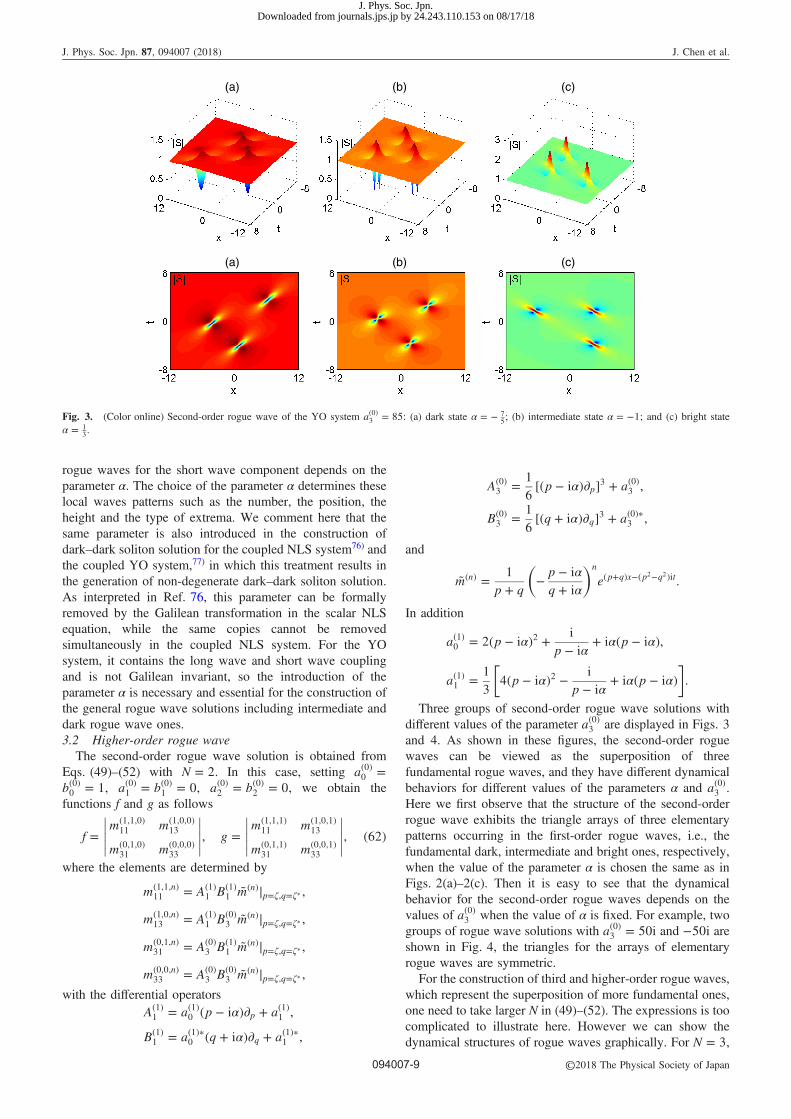
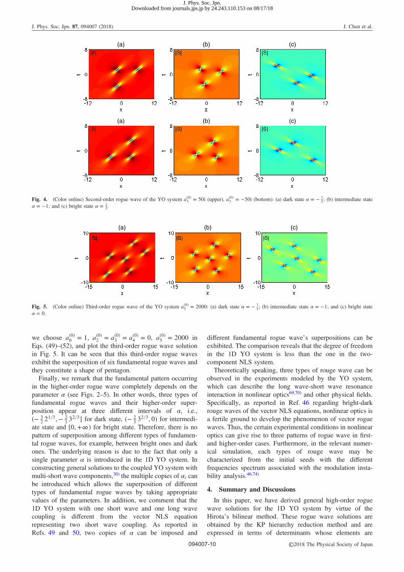
Three groups of second-order rogue wave solutions withdifferent values of the parameter að0Þ3 are displayed in Figs. 3and 4. As shown in these figures, the second-order roguewaves can be viewed as the superposition of threefundamental rogue waves, and they have different dynamicalbehaviors for different values of the parameters α and að0Þ3 .Here we first observe that the structure of the second-orderrogue wave exhibits the triangle arrays of three elementarypatterns occurring in the first-order rogue waves, i.e., thefundamental dark, intermediate and bright ones, respectively,when the value of the parameter α is chosen the same as inFigs. 2(a)–2(c). Then it is easy to see that the dynamicalbehavior for the second-order rogue waves depends on thevalues of að0Þ3 when the value of α is fixed. For example, twogroups of rogue wave solutions with að0Þ3 ¼ 50i and �50i areshown in Fig. 4, the triangles for the arrays of elementaryrogue waves are symmetric.

For the construction of third and higher-order rogue waves,which represent the superposition of more fundamental ones,one need to take larger N in (49)–(52). The expressions is toocomplicated to illustrate here. However we can show thedynamical structures of rogue waves graphically. For N ¼ 3,

(a) (b) (c)

(a) (b) (c)

Fig. 3. (Color online) Second-order rogue wave of the YO system að0Þ3 ¼ 85: (a) dark state � ¼ � 75; (b) intermediate state � ¼ �1; and (c) bright state

� ¼ 13.

J. Phys. Soc. Jpn. 87, 094007 (2018) J. Chen et al.

094007-9 ©2018 The Physical Society of Japan

J. Phys. Soc. Jpn.Downloaded from journals.jps.jp by 24.243.110.153 on 08/17/18

we choose að0Þ0 ¼ 1, að0Þ2 ¼ að0Þ3 ¼ að0Þ4 ¼ 0, að0Þ5 ¼ 2000 inEqs. (49)–(52), and plot the third-order rogue wave solutionin Fig. 5. It can be seen that this third-order rogue wavesexhibit the superposition of six fundamental rogue waves andthey constitute a shape of pentagon.

Finally, we remark that the fundamental pattern occurringin the higher-order rogue wave completely depends on theparameter α (see Figs. 2–5). In other words, three types offundamental rogue waves and their higher-order super-position appear at three different intervals of α, i.e.,ð� 3

221=3;� 2

332=3� for dark state, ð� 2

332=3; 0Þ for intermedi-

ate state and ½0;þ1Þ for bright state. Therefore, there is nopattern of superposition among different types of fundamen-tal rogue waves, for example, between bright ones and darkones. The underlying reason is due to the fact that only asingle parameter α is introduced in the 1D YO system. Inconstructing general solutions to the coupled YO system withmulti-short wave components,30) the multiple copies of �i canbe introduced which allows the superposition of differenttypes of fundamental rogue waves by taking appropriatevalues of the parameters. In addition, we comment that the1D YO system with one short wave and one long wavecoupling is different from the vector NLS equationrepresenting two short wave coupling. As reported inRefs. 49 and 50, two copies of α can be imposed and

different fundamental rogue wave’s superpositions can beexhibited. The comparison reveals that the degree of freedomin the 1D YO system is less than the one in the two-component NLS system.

Theoretically speaking, three types of rouge wave can beobserved in the experiments modeled by the YO system,which can describe the long wave-short wave resonanceinteraction in nonlinear optics69,70) and other physical fields.Specifically, as reported in Ref. 46 regarding bright-darkrouge waves of the vector NLS equations, nonlinear optics isa fertile ground to develop the phenomenon of vector roguewaves. Thus, the certain experimental conditions in nonlinearoptics can give rise to three patterns of rogue wave in first-and higher-order cases. Furthermore, in the relevant numer-ical simulation, each types of rouge wave may becharacterized from the initial seeds with the differentfrequencies spectrum associated with the modulation insta-bility analysis.46,74)

4. Summary and Discussions

In this paper, we have derived general high-order roguewave solutions for the 1D YO system by virtue of theHirota’s bilinear method. These rogue wave solutions areobtained by the KP hierarchy reduction method and areexpressed in terms of determinants whose elements are

(a) (b) (c)

Fig. 5. (Color online) Third-order rogue wave of the YO system að0Þ5 ¼ 2000: (a) dark state � ¼ � 75; (b) intermediate state � ¼ �1; and (c) bright state

� ¼ 0.

(a) (b) (c)

(a) (b) (c)

Fig. 4. (Color online) Second-order rogue wave of the YO system að0Þ3 ¼ 50i (upper), að0Þ3 ¼ �50i (bottom): (a) dark state � ¼ � 75; (b) intermediate state

� ¼ �1; and (c) bright state � ¼ 13.

J. Phys. Soc. Jpn. 87, 094007 (2018) J. Chen et al.

094007-10 ©2018 The Physical Society of Japan

J. Phys. Soc. Jpn.Downloaded from journals.jps.jp by 24.243.110.153 on 08/17/18

algebraic formulae. By choosing different values of parame-ters in the rogue wave solutions, we have analytically andgraphically studied the dynamics of first-order, second-order,and third-order rogue wave solutions. As a result, thefundamental (first-order) rogue waves have been classifiedinto three different patterns: bright, intermediate and darkstates. The higher-order rogue waves correspond to thesuperposition of fundamental rogue waves. In particular,we should mention here that, in compared with the NLSequation, there exists an essential parameter α to control thepattern of rogue wave for both first- and higher-order roguewaves since the YO system does not possess the Galileaninvariance.

Apart from rogue waves appearing in the continuousmodels, the behavior of rogue waves in discrete systems haverecently drawn much attention.31–33) Paralleling to the novelpatterns of rogue waves such as dark and intermediate ones inthe continuous coupled systems with multiple waves, thediscrete counterparts of such rogue waves can be attained indiscrete systems. We have recently proposed an integrablesemi-discrete analogue of the 1D YO system.78) Thus thesemi-discrete rogue wave, especially the semi-discrete darkand intermediate ones are worthy to be expected. We willreport the results on this topic in the future.

Acknowledgments JC’s work was supported from the National NaturalScience Foundation of China (NSFC) (No. 11705077). YC’s work was supportedfrom the Global Change Research Program of China (No. 2015CB953904),NSFC (Nos. 11675054 and 11435005) and Shanghai Collaborative InnovationCenter of Trustworthy Software for Internet of Things (No. ZF1213). BF’s workwas partially supported by National Science Foundation (DMS-1715991) andNSFC for Overseas Scholar Collaboration Research (No. 11728103). KM’s workwas supported by JSPS Grant-in-Aid for Scientific Research (C-15K04909) andJST CREST. YO’s work was partially supported by JSPS Grant-in-Aid forScientific Research (B-24340029, S-24224001, C-15K04909) and for Challeng-ing Exploratory Research (26610029).

+ychen@sei.ecnu.edu.cn†baofeng.feng@utrgv.edu‡kmaruno@waseda.jp§ohta@math.kobe-u.ac.jp1) C. Kharif, E. Pelinovsky, and A. Slunyaev, Rogue Waves in the Ocean

(Springer, Berlin, 2009).2) D. R. Solli, C. Ropers, P. Koonath, and B. Jalali, Nature 450, 1054

(2007).3) R. Höhmann, U. Kuhl, H. J. Stöckmann, L. Kaplan, and E. J. Heller,

Phys. Rev. Lett. 104, 093901 (2010).4) A. Montina, U. Bortolozzo, S. Residori, and F. T. Arecchi, Phys. Rev.

Lett. 103, 173901 (2009).5) Y. V. Bludov, V. V. Konotop, and N. Akhmediev, Phys. Rev. A 80,

033610 (2009).6) Y. V. Bludov, V. V. Konotop, and N. Akhmediev, Eur. Phys. J.: Spec.

Top. 185, 169 (2010).7) A. N. Ganshin, V. B. Efimov, G. V. Kolmakov, L. P. Mezhov-Deglin,

and P. V. E. McClintock, Phys. Rev. Lett. 101, 065303 (2008).8) L. Stenflo and M. Marklund, J. Plasma Phys. 76, 293 (2010).9) W. M. Moslem, Phys. Plasmas 18, 032301 (2011).10) H. Bailung, S. K. Sharma, and Y. Nakamura, Phys. Rev. Lett. 107,

255005 (2011).11) M. Shats, H. Punzmann, and H. Xia, Phys. Rev. Lett. 104, 104503

(2010).12) Z. Y. Yan, Phys. Lett. A 375, 4274 (2011).13) N. Akhmediev, A. Ankiewicz, and M. Taki, Phys. Lett. A 373, 675

(2009).14) N. Akhmediev, J. M. Soto-Crespo, and A. Ankiewicz, Phys. Lett. A

373, 2137 (2009).15) D. H. Peregrine, J. Aust. Math. Soc., Ser. B 25, 16 (1983).16) N. Akhmediev, A. Ankiewicz, and J. M. Soto-Crespo, Phys. Rev. E 80,

026601 (2009).17) D. J. Kedziora, A. Ankiewicz, and N. Akhmediev, Phys. Rev. E 85,

066601 (2012).18) A. Ankiewicz, D. J. Kedziora, and N. Akhmediev, Phys. Lett. A 375,

2782 (2011).19) D. J. Kedziora, A. Ankiewicz, and N. Akhmediev, Phys. Rev. E 84,

056611 (2011).20) P. Dubard, P. Gaillard, C. Klein, and V. B. Matveev, Eur. Phys. J.:

Spec. Top. 185, 247 (2010).21) P. Dubard and V. B. Matveev, Nat. Hazards Earth Syst. Sci. 11, 667

(2011).22) P. Gaillard, J. Phys. A 44, 435204 (2011).23) B. L. Guo, L. M. Ling, and Q. P. Liu, Phys. Rev. E 85, 026607 (2012).24) Y. Ohta and J. K. Yang, Proc. R. Soc. London, Ser. A 468, 1716

(2012).25) A. Ankiewicz, J. M. Soto-Crespo, and N. Akhmediev, Phys. Rev. E 81,

046602 (2010).26) J. S. He, H. R. Zhang, L. H. Wang, K. Porsezian, and A. S. Fokas,

Phys. Rev. E 87, 052914 (2013).27) G. Mu and Z. Y. Qin, Nonlinear Anal.: Real World Appl. 31, 179

(2016).28) L. M. Ling, B. F. Feng, and Z. N. Zhu, Physica D 327, 13 (2016).29) L. Wang, D. Y. Jiang, F. H. Qi, Y. Y. Shi, and Y. C. Zhao, Commun.

Nonlinear Sci. Numer. Simulation 42, 502 (2017).30) J. C. Chen, Y. Chen, B. F. Feng, and K. Maruno, Phys. Lett. A 379,

1510 (2015).31) Y. V. Bludov, V. V. Konotop, and N. Akhmediev, Phys. Rev. E 34,

2015 (2009).32) A. Ankiewicz, N. Akhmediev, and J. M. Soto-Crespo, Phys. Rev. E 82,

026602 (2010).33) Y. Ohta and J. K. Yang, J. Phys. A 47, 255201 (2014).34) Z. Y. Yan, Phys. Lett. A 374, 672 (2010).35) Z. Y. Yan, V. V. Konotop, and N. Akhmediev, Phys. Rev. E 82,

036610 (2010).36) Z. Y. Yan and C. Q. Dai, J. Opt. 15, 064012 (2013).37) X. Y. Wen, Y. Q. Yang, and Z. Y. Yan, Phys. Rev. E 92, 012917

(2015).38) Z. Y. Yan, Nonlinear Dyn. 79, 2515 (2015).39) Y. Q. Yang, Z. Y. Yan, and B. A. Malomed, Chaos 25, 103112 (2015).40) X. Y. Wen, Z. Y. Yan, and Y. Q. Yang, Chaos 26, 063123 (2016).41) X. Y. Wen and Z. Y. Yan, Commun. Nonlinear Sci. Numer. Simulation

43, 311 (2017).42) A. Chabchoub and N. Akhmediev, Phys. Lett. A 377, 2590 (2013).43) A. Chabchoub, N. Hoffmann, M. Onorato, A. Slunyaev, A. Sergeeva,

E. Pelinovsky, and N. Akhmediev, Phys. Rev. E 86, 056601 (2012).44) L. M. Ling, B. L. Guo, and L. C. Zhao, Phys. Rev. E 89, 041201

(2014).45) B. L. Guo and L. M. Ling, Chin. Phys. Lett. 28, 110202 (2011).46) F. Baronio, A. Degasperis, M. Conforti, and S. Wabnitz, Phys. Rev.

Lett. 109, 044102 (2012).47) L. C. Zhao and J. Liu, Phys. Rev. E 87, 013201 (2013).48) F. Baronio, M. Conforti, A. Degasperis, and S. Lombardo, Phys. Rev.

Lett. 111, 114101 (2013).49) L. C. Zhao, B. L. Guo, and L. M. Ling, J. Math. Phys. 57, 043508

(2016).50) L. M. Ling, L. C. Zhao, and B. L. Guo, Commun. Nonlinear Sci.

Numer. Simulation 32, 285 (2016).51) G. Mu, Z. Y. Qin, and R. Grimshaw, SIAM J. Appl. Math. 75, 1

(2015).52) J. Wei, X. Wang, and X. G. Geng, Commun. Nonlinear Sci. Numer.

Simulation 59, 1 (2018).53) X. Wang, Y. Q. Li, F. Huang, and Y. Chen, Commun. Nonlinear Sci.

Numer. Simulation 20, 434 (2015).54) Y. Zhang, J. W. Yang, K. W. Chow, and C. F. Wu, Nonlinear Anal.:

Real World Appl. 33, 237 (2017).55) Y. Ohta and J. K. Yang, Phys. Rev. E 86, 036604 (2012).56) Y. Ohta and J. K. Yang, J. Phys. A 46, 105202 (2013).57) G. Mu and Z. Y. Qin, Nonlinear Anal.: Real World Appl. 18, 1 (2014).58) X. Y. Wen and Z. Y. Yan, Chaos 25, 123115 (2015).59) X. Y. Wen, Z. Y. Yan, and B. A. Malomed, Chaos 26, 123110 (2016).60) D. J. Benney, Stud. Appl. Math. 55, 93 (1976).61) D. J. Benney, Stud. Appl. Math. 56, 81 (1977).62) V. E. Zakharov, Sov. Phys. JETP 35, 908 (1972).

J. Phys. Soc. Jpn. 87, 094007 (2018) J. Chen et al.

094007-11 ©2018 The Physical Society of Japan

J. Phys. Soc. Jpn.Downloaded from journals.jps.jp by 24.243.110.153 on 08/17/18

63) N. Yajima and M. Oikawa, Prog. Theor. Phys. 56, 1719 (1976).64) V. D. Djordjevic and L. G. Redekopp, J. Fluid Mech. 79, 703 (1977).65) R. H. J. Grimshaw, Stud. Appl. Math. 56, 241 (1977).66) M. Funakoshi and M. Oikawa, J. Phys. Soc. Jpn. 52, 1982 (1983).67) Y. C. Ma and L. G. Redekopp, Phys. Fluids 22, 1872 (1979).68) Y. C. Ma, Stud. Appl. Math. 59, 201 (1978).69) Y. S. Kivshar, Opt. Lett. 17, 1322 (1992).70) A. Chowdhury and J. A. Tataronis, Phys. Rev. Lett. 100, 153905

(2008).71) Y. Cheng, J. Math. Phys. 33, 3774 (1992).72) I. Loris and R. Willox, Inverse Probl. 13, 411 (1997).

73) K. W. Chow, H. N. Chan, D. J. Kedziora, and R. H. J. Grimshaw,J. Phys. Soc. Jpn. 82, 074001 (2013).

74) S. H. Chen, P. Grelu, and J. M. Soto-Crespo, Phys. Rev. E 89, 011201(2014).

75) S. H. Chen, Phys. Lett. A 378, 1095 (2014).76) Y. Ohta, D. S. Wang, and J. K. Yang, Stud. Appl. Math. 127, 345

(2011).77) J. C. Chen, Y. Chen, B. F. Feng, and K. Maruno, J. Phys. Soc. Jpn. 84,

034002 (2015).78) J. C. Chen, Y. Chen, B.-F. Feng, K. Maruno, and Y. Ohta, J. Phys. A

49, 165201 (2016).

J. Phys. Soc. Jpn. 87, 094007 (2018) J. Chen et al.

094007-12 ©2018 The Physical Society of Japan

J. Phys. Soc. Jpn.Downloaded from journals.jps.jp by 24.243.110.153 on 08/17/18