Embed Size (px)
Citation preview
1
General Equilibrium Analysis with StochasticBenchmarking
Qi Shang
Department of FinanceLondon School of Economics
Houghton StreetLondon WC2A 2AE
Email: [email protected]
First Version: August 2008This Version: March 2009
Abstract: This paper applies a continuous-time model to study the equilibrium of aneconomy consisting one normal agent and one constrained agent who has to maintain hisintermediate wealth above a stochastic benchmark whose value is determined endogenously.After characterizing the optimization problems, I use the martingale approach to derive theequilibrium market dynamics in closed-form to compare with the normal economy. In thebenchmarking economy before the constraint date, asset price, volatility and risk premiumare higher than those in the normal economy for risky benchmarks. When the benchmarkis relatively safe, asset price is higher but volatility, risk premium and the optimal fractionof wealth invested in the risky asset are decreased.
2
This paper studies the effect of a portfolio benchmarking constraint on the equilibrium
market dynamics. The economy has a normal agent with log utility over continuous con-
sumption and a constrained agent (also with log utility) whose intermediate wealth must
be no less than a stochastic benchmarking constraint. Using the martingale approach, I
solve this continuous-time consumption-based general equilibrium model explicitly to get
the equilibrium assets prices, risk premium, volatility, optimal strategy and compare them
with those in a normal economy. To my knowledge, this is the first paper to investigate
the equilibrium effects of this benchmarking constraint.
The constraint studied here is a requirement that an agent’s wealth is no less than a
stochastic benchmark index, whose parameters are exogenously given but the value of this
benchmark is determined endogenously. The problem of beating a constant floor has been
studied by the portfolio insurance literature, e.g. the equilibrium analysis of portfolio in-
surance by Basak (1995) and Grossman and Zhou (1996). However, the portfolio insurance
constraint only ensures the agent doesn’t lose more than a certain level without asking for
a high return when the state is good. The inclusion of a stochastic benchmark index in the
stochastic benchmarking constraint means the agent’s performance has to beat the index
when market does well and therefore, imposing such a constraint on agent ensures good
performance. Since there are only two assets in the economy, a risk-free asset and a risky
stock, and markets are complete, the stochastic benchmark is a replication portfolio using
the bond and stock. Then, the riskiness of the benchmark is measured by the positions in
the risk-free asset. Since the benchmark index is achievable through passive management,
it is considered as the minimum return that is required for active portfolio management.
After describing the economy, which apart from the existence of the constraint is the stan-
dard set-up following Lucas (1978), I first characterize the portfolio choice problems for the
3
normal agent and the constrained agent. The approach is the martingale representation
approach as in Cox and Huang (1989) and Basak (1995). Then I get explicit solutions for
the equilibrium market dynamics using the martingale approach for option pricing and Ito’s
lemma. Similar procedure has been used by Basak (1995) but the alternative consideration
of the stochastic benchmark complicates the discussion of equilibrium effects.
I find that in the stochastic benchmarking economy before the constraint date, the risky
asset price is higher than that in the normal economy because the constrained agent con-
sumes less than if he’s not constrained. Since the risk-free asset is in zero net supply, the
extra investment from the constrained agent goes into the risky asset market and drives up
the risky asset’s price. After the constraint date, there’s no effect. The increase in stock
price also reflects the agent’s preference for consumption and dividend after the constraint
date. When the benchmark is risky, which means the replication portfolio has a short
position on the risk-free asset, then the risk premium, volatility, and the optimal fraction
of wealth invested in the risky asset by the constrained agent are increased by the presence
of the constraint. While if the benchmark is relatively safe, i.e. the replication portfolio
contains positive position in the risk-free asset, then the risk premium, volatility, and the
optimal fraction of wealth invested in the risky asset by the constrained agent are always
decreased by the presence of the constraint. In both cases, the degree of the effects are
state-dependent.
The rationale behind these findings is when there are more (less) demand for the risky
asset from the constrained agent, the volatility has to increase (decrease) so as to clear the
market. It is also because that the stock price in this economy is equal to the normal econ-
omy price plus the present value of an option-like payoff that represents the effects from
the benchmarking constraint. For the risky benchmark case, the extra payoff is like a call
4
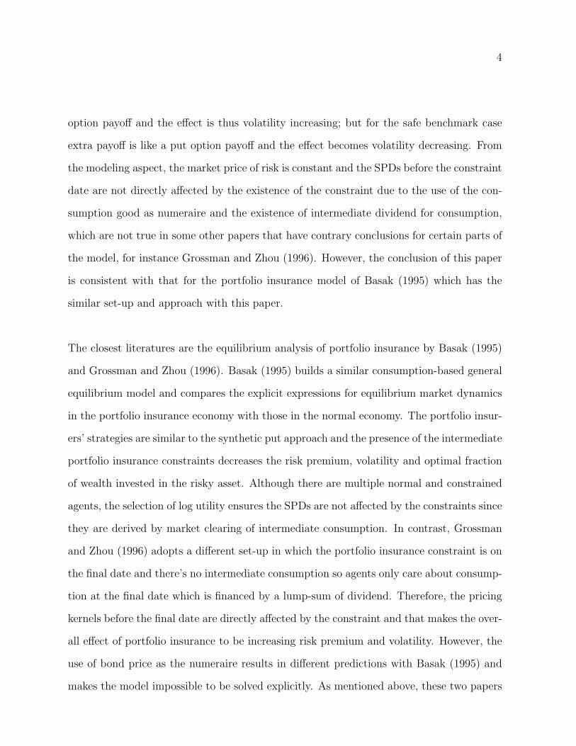
option payoff and the effect is thus volatility increasing; but for the safe benchmark case
extra payoff is like a put option payoff and the effect becomes volatility decreasing. From
the modeling aspect, the market price of risk is constant and the SPDs before the constraint
date are not directly affected by the existence of the constraint due to the use of the con-
sumption good as numeraire and the existence of intermediate dividend for consumption,
which are not true in some other papers that have contrary conclusions for certain parts of
the model, for instance Grossman and Zhou (1996). However, the conclusion of this paper
is consistent with that for the portfolio insurance model of Basak (1995) which has the
similar set-up and approach with this paper.
The closest literatures are the equilibrium analysis of portfolio insurance by Basak (1995)
and Grossman and Zhou (1996). Basak (1995) builds a similar consumption-based general
equilibrium model and compares the explicit expressions for equilibrium market dynamics
in the portfolio insurance economy with those in the normal economy. The portfolio insur-
ers’ strategies are similar to the synthetic put approach and the presence of the intermediate
portfolio insurance constraints decreases the risk premium, volatility and optimal fraction
of wealth invested in the risky asset. Although there are multiple normal and constrained
agents, the selection of log utility ensures the SPDs are not affected by the constraints since
they are derived by market clearing of intermediate consumption. In contrast, Grossman
and Zhou (1996) adopts a different set-up in which the portfolio insurance constraint is on
the final date and there’s no intermediate consumption so agents only care about consump-
tion at the final date which is financed by a lump-sum of dividend. Therefore, the pricing
kernels before the final date are directly affected by the constraint and that makes the over-
all effect of portfolio insurance to be increasing risk premium and volatility. However, the
use of bond price as the numeraire results in different predictions with Basak (1995) and
makes the model impossible to be solved explicitly. As mentioned above, these two papers
5
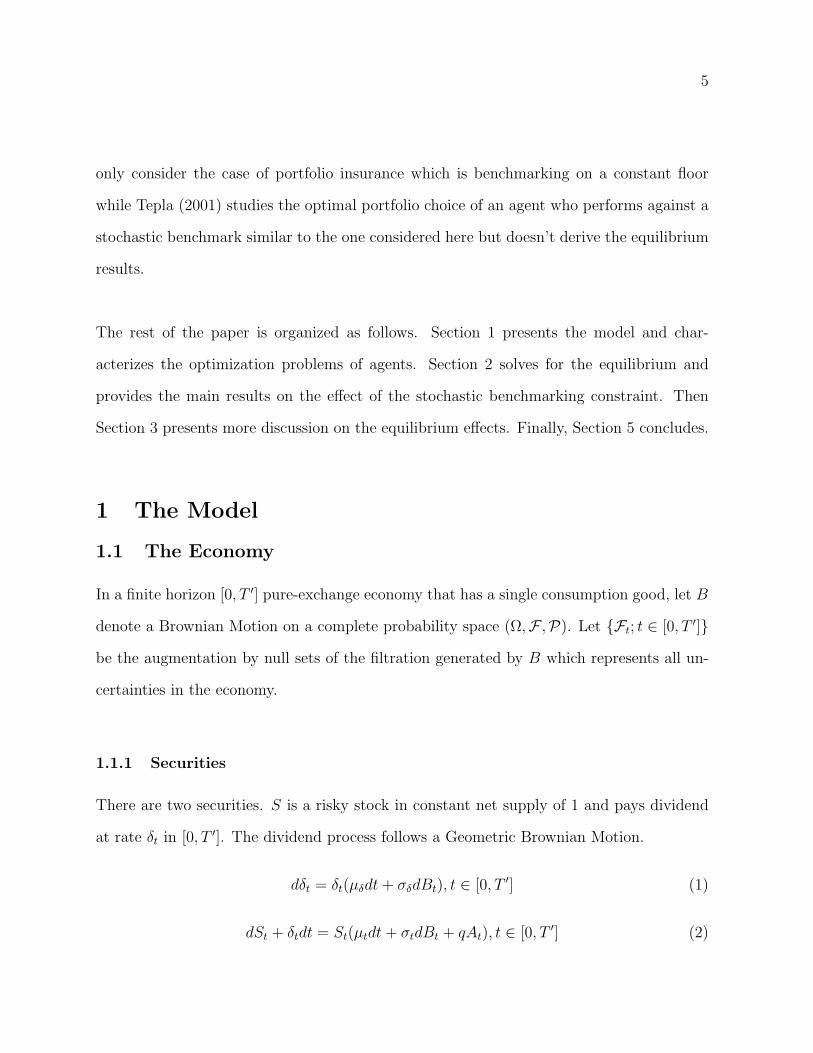
only consider the case of portfolio insurance which is benchmarking on a constant floor
while Tepla (2001) studies the optimal portfolio choice of an agent who performs against a
stochastic benchmark similar to the one considered here but doesn’t derive the equilibrium
results.
The rest of the paper is organized as follows. Section 1 presents the model and char-
acterizes the optimization problems of agents. Section 2 solves for the equilibrium and
provides the main results on the effect of the stochastic benchmarking constraint. Then
Section 3 presents more discussion on the equilibrium effects. Finally, Section 5 concludes.
1 The Model
1.1 The Economy
In a finite horizon [0, T ′] pure-exchange economy that has a single consumption good, let B
denote a Brownian Motion on a complete probability space (Ω,F ,P). Let Ft; t ∈ [0, T ′]
be the augmentation by null sets of the filtration generated by B which represents all un-
certainties in the economy.
1.1.1 Securities
There are two securities. S is a risky stock in constant net supply of 1 and pays dividend
at rate δt in [0, T ′]. The dividend process follows a Geometric Brownian Motion.
dδt = δt(µδdt + σδdBt), t ∈ [0, T ′] (1)
dSt + δtdt = St(µtdt + σtdBt + qAt), t ∈ [0, T ′] (2)
6
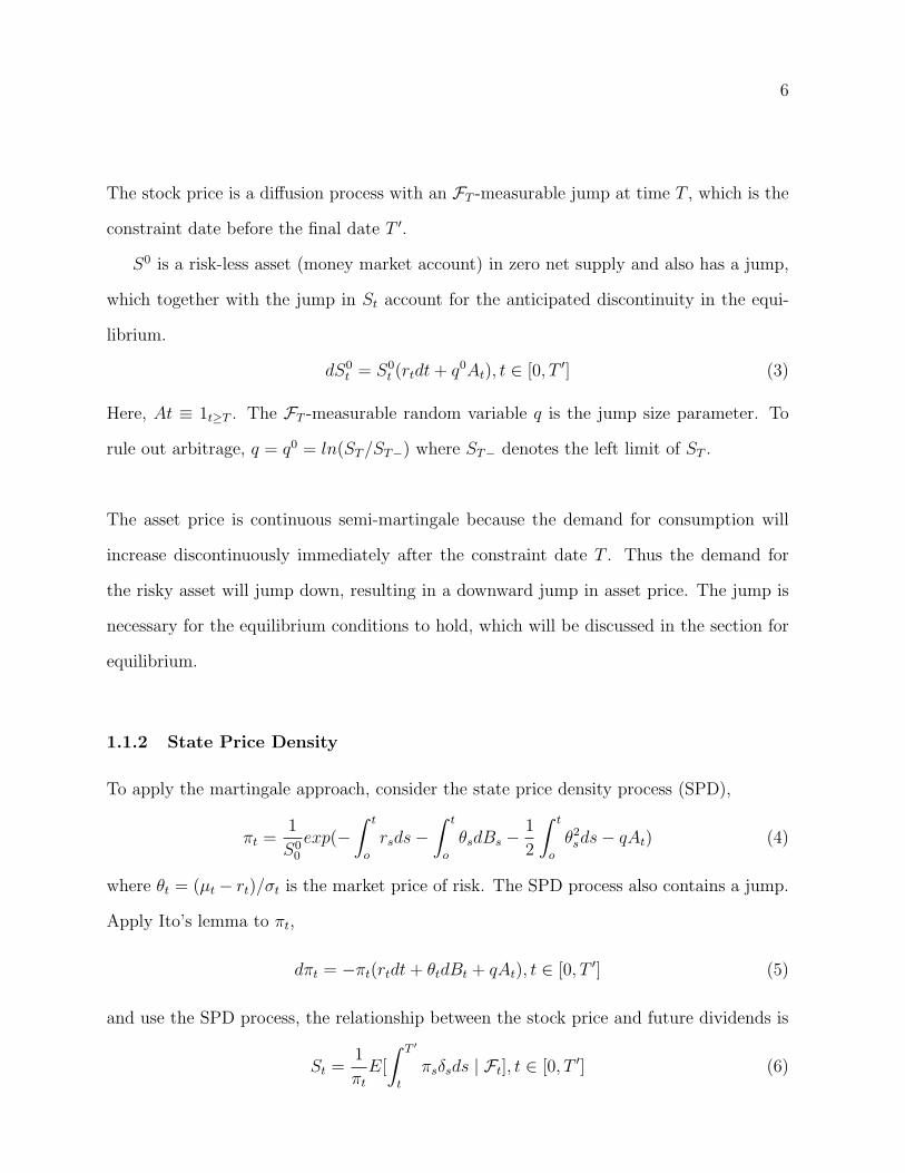
The stock price is a diffusion process with an FT -measurable jump at time T , which is the
constraint date before the final date T ′.
S0 is a risk-less asset (money market account) in zero net supply and also has a jump,
which together with the jump in St account for the anticipated discontinuity in the equi-
librium.
dS0t = S0
t (rtdt + q0At), t ∈ [0, T ′] (3)
Here, At ≡ 1t≥T . The FT -measurable random variable q is the jump size parameter. To
rule out arbitrage, q = q0 = ln(ST /ST−) where ST− denotes the left limit of ST .
The asset price is continuous semi-martingale because the demand for consumption will
increase discontinuously immediately after the constraint date T . Thus the demand for
the risky asset will jump down, resulting in a downward jump in asset price. The jump is
necessary for the equilibrium conditions to hold, which will be discussed in the section for
equilibrium.
1.1.2 State Price Density
To apply the martingale approach, consider the state price density process (SPD),
πt =1
S00
exp(−∫ t
o
rsds−∫ t
o
θsdBs −1
2
∫ t
o
θ2sds− qAt) (4)
where θt = (µt − rt)/σt is the market price of risk. The SPD process also contains a jump.
Apply Ito’s lemma to πt,
dπt = −πt(rtdt + θtdBt + qAt), t ∈ [0, T ′] (5)
and use the SPD process, the relationship between the stock price and future dividends is
St =1
πt
E[
∫ T ′
t
πsδsds | Ft], t ∈ [0, T ′] (6)
7
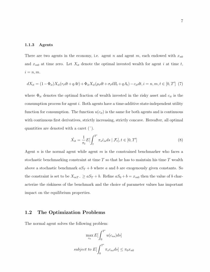
1.1.3 Agents
There are two agents in the economy, i.e. agent n and agent m, each endowed with xn0
and xm0 at time zero. Let Xit denote the optimal invested wealth for agent i at time t,
i = n, m.
dXit = (1−Φit)Xit(rtdt+qAt)+ΦitXit(µtdt+σtdBt +qAt)−citdt, i = n, m, t ∈ [0, T ′] (7)
where Φit denotes the optimal fraction of wealth invested in the risky asset and cit is the
consumption process for agent i. Both agents have a time-additive state-independent utility
function for consumption. The function u(cit) is the same for both agents and is continuous
with continuous first derivatives, strictly increasing, strictly concave. Hereafter, all optimal
quantities are denoted with a caret (ˆ).
Xit =1
πt
E[
∫ T ′
t
πscisds | Ft], t ∈ [0, T ′] (8)
Agent n is the normal agent while agent m is the constrained benchmarker who faces a
stochastic benchmarking constraint at time T so that he has to maintain his time T wealth
above a stochastic benchmark aST + b where a and b are exogenously given constants. So
the constraint is set to be XmT− ≥ aST + b. Refine aS0 + b = xm0 then the value of b char-
acterize the riskiness of the benchmark and the choice of parameter values has important
impact on the equilibrium properties.
1.2 The Optimization Problems
The normal agent solves the following problem:
maxcn
E[
∫ T ′
0
u(cns)ds]
subject to E[
∫ T ′
0
πscnsds] ≤ π0xn0

8
Assuming a solution exists, the solution is:
cnt = I(λnπt) t ∈ [0, T ′] (9)
where I(·) is the inverse of u′(·) and λn solves:
E[
∫ T ′
0
πsI(λnπs)ds] = π0xn0 (10)
The constrained agent m solves:
maxcm,XmT−
E[
∫ T ′
0
u(cms)ds]
subject to E[
∫ T
0
πscmsds + πT−XmT−] ≤ π0xn0
E[
∫ T ′
T
πscmsds | FT ] ≤ πT−xmT− almost surely,
XmT− ≥ aST + b almost surely
Lemma 1.
Assuming a solution exists, the solution is:
cmt = I(λm1πt) t ∈ [0, T ) (11)
cmt = I(λm2πt) t ∈ [T, T ′] (12)
where λm1 and λm2 solve:
E[
∫ T
0
πsI(λm1πs)ds + πT− maxaST + b,1
πT−E[
∫ T ′
T
πsI(λm1πs)ds|FT ]] = π0xm0 (13)
E[
∫ T ′
T
πsI(λm2πs)ds|FT ] = πT− maxaST + b,1
πT−E[
∫ T ′
T
πsI(λm1πs)ds|FT ] (14)
N.B.(1) λn, λm1 are constant, λm2 is FT -measurable random variable. (2) If xn0 = xm0, then
λm1 ≥ λn. (3) λm1 = λm2 if the benchmarking constraint is not binding and λm1 > λm2 if
9
it is binding.
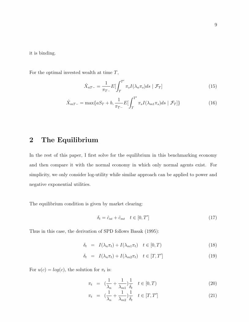
For the optimal invested wealth at time T ,
XnT− =1
πT−E[
∫ T ′
T
πsI(λnπs)ds | FT ] (15)
XmT− = maxaST + b,1
πT−E[
∫ T ′
T
πsI(λm1πs)ds | FT ] (16)
2 The Equilibrium
In the rest of this paper, I first solve for the equilibrium in this benchmarking economy
and then compare it with the normal economy in which only normal agents exist. For
simplicity, we only consider log-utility while similar approach can be applied to power and
negative exponential utilities.
The equilibrium condition is given by market clearing:
δt = cnt + cmt t ∈ [0, T ′] (17)
Thus in this case, the derivation of SPD follows Basak (1995):
δt = I(λnπt) + I(λm1πt) t ∈ [0, T ) (18)
δt = I(λnπt) + I(λm2πt) t ∈ [T, T ′] (19)
For u(c) = log(c), the solution for πt is:
πt = (1
λn
+1
λm1
)1
δt
t ∈ [0, T ) (20)
πt = (1
λn
+1
λm2
)1
δt
t ∈ [T, T ′] (21)
10
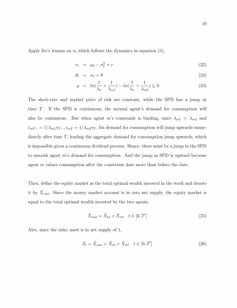
Apply Ito’s lemma on πt which follows the dynamics in equation (5),
rt = µδ − σ2δ = r (22)
θt = σδ = θ (23)
q = ln(1
λn
+1
λm1
)− ln(1
λn
+1
λm2
) ≤ 0 (24)
The short-rate and market price of risk are constant, while the SPD has a jump at
time T . If the SPD is continuous, the normal agent’s demand for consumption will
also be continuous. But when agent m’s constraint is binding, since λm1 > λm2 and
cmT− = 1/λm1πT−, cmT = 1/λm2πT , his demand for consumption will jump upwards imme-
diately after time T , leading the aggregate demand for consumption jump upwards, which
is impossible given a continuous dividend process. Hence, there must be a jump in the SPD
to smooth agent m’s demand for consumption. And the jump in SPD is upward because
agent m values consumption after the constraint date more than before the date.
Then, define the equity market as the total optimal wealth invested in the stock and denote
it by Xemt. Since the money market account is in zero net supply, the equity market is
equal to the total optimal wealth invested by the two agents.
Xemt = Xnt + Xmt t ∈ [0, T ′] (25)
Also, since the risky asset is in net supply of 1,
St = Xemt = Xnt + Xmt t ∈ [0, T ′] (26)
11
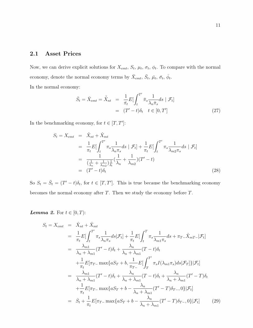
2.1 Asset Prices
Now, we can derive explicit solutions for Xemt, St, µt, σt, φt. To compare with the normal
economy, denote the normal economy terms by Xemt, St, µt, σt, φt.
In the normal economy:
St = Xemt =¯Xnt =
1
πt
E[
∫ T ′
t
πs1
λnπs
ds | Ft]
= (T ′ − t)δt t ∈ [0, T ′] (27)
In the benchmarking economy, for t ∈ [T, T ′]:
St = Xemt = Xnt + Xmt
=1
πt
E[
∫ T ′
t
πs1
λnπs
ds | Ft] +1
πt
E[
∫ T ′
t
πs1
λm2πs
ds | Ft]
=1
( 1λn
+ 1λm2
) 1δt
(1
λn
+1
λm2
)(T ′ − t)
= (T ′ − t)δt (28)
So St = St = (T ′ − t)δt, for t ∈ [T, T ′]. This is true because the benchmarking economy
becomes the normal economy after T . Then we study the economy before T .
Lemma 2. For t ∈ [0, T ):
St = Xemt = Xnt + Xmt
=1
πt
E[
∫ T ′
t
πs1
λnπs
ds|Ft] +1
πt
E[
∫ T
t
πs1
λm1πs
ds + πT−XmT−|Ft]
=λm1
λn + λm1
(T ′ − t)δt +λn
λn + λm1
(T − t)δt
+1
πt
E[πT− maxaST + b,1
πT−E[
∫ T ′
T
πsI(λm1πs)ds|FT ]|Ft]
=λm1
λn + λm1
(T ′ − t)δt +λn
λn + λm1
(T − t)δt +λn
λn + λm1
(T ′ − T )δt
+1
πt
E[πT− maxaST + b− λn
λn + λm1
(T ′ − T )δT−, 0|Ft]
= St +1
πt
E[πT− maxaST + b− λn
λn + λm1
(T ′ − T )δT−, 0|Ft] (29)

12
N.B. St ≥ St, for t ∈ [0, T ). This is true because before time T agent m consumes less
than if he’s unconstrained. So he invests more than he would if unconstrained. Since the
risk-free asset is in zero net supply, the extra investment from agent m goes into the stock
market and drives the price up before time T .
Now focus on the explicit solution of St for t ∈ [0, T ). From the equation (28), ST =
(T ′ − T )δT , and by the continuity of δt, δT− = δT . So, replace ST by (T ′ − T )δT−, rewrite
equation (29) as:
St = (T ′ − t)δt +1
πt
E[πT− max(a− λn
λn + λm1
)(T ′ − T )δT− + b, 0|Ft] (30)
Since the process δt is a Geometric Brownian Motion, we can apply the martingale ap-
proach to take the expectation in equation (30). Hereafter, we assume (a − λn
λn+λm1)b < 0
which means there’s uncertainty over the relative performance of the benchmark and the
unconstrained strategy. Now, solve equation (30), we have:
Proposition 1. In the benchmarking economy,
St = (T ′ − t)δt + (a− λn
λn + λm1
)(T ′ − T )N(z1)δt + be−r(T−t)N(z2) (31)
where
z1 = z2 + σδ
√T − t
z2 =ln[(a− λn
λn+λm1)(T ′ − T )δt/− b] + (r − 1
2σ2
δ )(T − t)
σδ
√T − t

13
N(·) is the distribution function of normal random variable. And we also have:
Xmt = St − Xnt = St −λm1
λn + λm1
(T ′ − t)δt (32)
2.2 Volatility and Risk Premium
Apply Ito’s lemma on St, we get explicit solutions for the volatility and risk premium in
both the normal and benchmarking economies.
Proposition 2.
In the normal economy, for t ∈ [0, T ′],
σt = σδ (33)
µt − r = σ2δ (34)
In the benchmarking economy, for t ∈ [T, T ′],
σt = σδ (35)
µt − r = σ2δ (36)
While for t ∈ [0, T ),
σt = [1− be−r(T−t)N(z2)
St
]σδ (37)
µt − r = [1− be−r(T−t)N(z2)
St
]σ2δ (38)
Whether the volatility and risk premium in the benchmarking economy are greater or
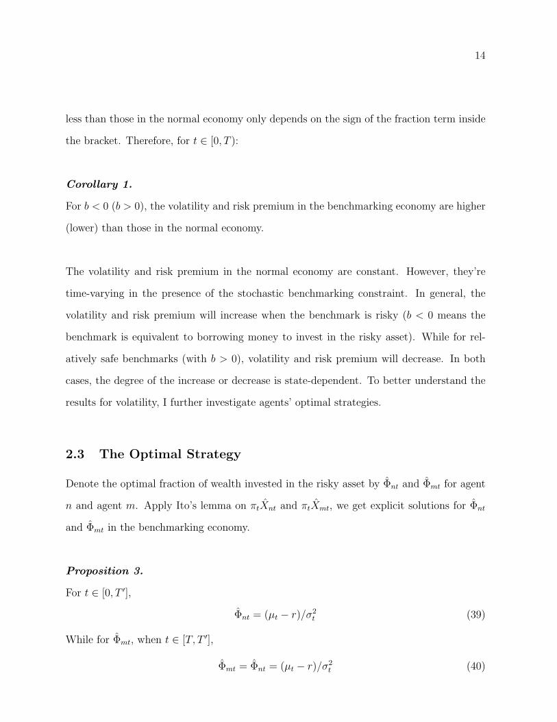
14
less than those in the normal economy only depends on the sign of the fraction term inside
the bracket. Therefore, for t ∈ [0, T ):
Corollary 1.
For b < 0 (b > 0), the volatility and risk premium in the benchmarking economy are higher
(lower) than those in the normal economy.
The volatility and risk premium in the normal economy are constant. However, they’re
time-varying in the presence of the stochastic benchmarking constraint. In general, the
volatility and risk premium will increase when the benchmark is risky (b < 0 means the
benchmark is equivalent to borrowing money to invest in the risky asset). While for rel-
atively safe benchmarks (with b > 0), volatility and risk premium will decrease. In both
cases, the degree of the increase or decrease is state-dependent. To better understand the
results for volatility, I further investigate agents’ optimal strategies.
2.3 The Optimal Strategy
Denote the optimal fraction of wealth invested in the risky asset by Φnt and Φmt for agent
n and agent m. Apply Ito’s lemma on πtXnt and πtXmt, we get explicit solutions for Φnt
and Φmt in the benchmarking economy.
Proposition 3.
For t ∈ [0, T ′],
Φnt = (µt − r)/σ2t (39)
While for Φmt, when t ∈ [T, T ′],
Φmt = Φnt = (µt − r)/σ2t (40)
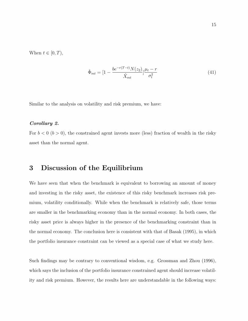
15
When t ∈ [0, T ),
Φmt = [1− be−r(T−t)N(z2)
Xmt
]µt − r
σ2t
(41)
Similar to the analysis on volatility and risk premium, we have:
Corollary 2.
For b < 0 (b > 0), the constrained agent invests more (less) fraction of wealth in the risky
asset than the normal agent.
3 Discussion of the Equilibrium
We have seen that when the benchmark is equivalent to borrowing an amount of money
and investing in the risky asset, the existence of this risky benchmark increases risk pre-
mium, volatility conditionally. While when the benchmark is relatively safe, those terms
are smaller in the benchmarking economy than in the normal economy. In both cases, the
risky asset price is always higher in the presence of the benchmarking constraint than in
the normal economy. The conclusion here is consistent with that of Basak (1995), in which
the portfolio insurance constraint can be viewed as a special case of what we study here.
Such findings may be contrary to conventional wisdom, e.g. Grossman and Zhou (1996),
which says the inclusion of the portfolio insurance constrained agent should increase volatil-
ity and risk premium. However, the results here are understandable in the following ways:
16
Firstly, seen from proposition 3 and corollary 2, the effect of volatility can be explained by
the optimal fraction of wealth invested in the stock by both agent. In the normal economy,
both agents optimally invest all their wealth into the stock (as implied by the log-utility).
In the safe benchmark case, the constrained agent has to invest less in the stock so as to
hold some risk-free asset. To clear the market, it means the unconstrained agent has to
take more than he would in the normal economy. Since we have,
Φnt = (µt − r)/σ2t = θ/σt (42)
so the only way to make the unconstrained agent be willing to hold more stock is to decrease
σt. While if the benchmark is risky, the constrained agent may have to hold more stock. So
the volatility has to increase to induce the unconstrained agent to sell. This suggests that
in this economy which has a constant market price of risk (θ), the volatility of the stock has
to decrease (increase) so as to make it more (less) attractive to the unconstrained agent.
In both case, since the constrained agent has to adjust his demand for the stock condition-
ally, the degree to which the volatility is increased or decreased is therefore state-dependent.
In another attempt to explain the effect on volatility, recall the expression for St before T in
equation (30). The stock price in the benchmarking economy is the normal economy price
plus an expectation term which is the present value of an option-like payoff, which is a call
option payoff when the benchmark is risky, and a put option payoff when the benchmark
is safe. For the safe benchmark case, when the market goes down, the put option value
goes up, which helps stabilize stock price. So the volatility is decreased in the presence
of the constraint. However, in the risky benchmark case, when the market goes down the
call option value goes down as well so the stock price falls even further and the constraint
increases volatility.
17
The results for the safe benchmark case is consistent with Basak (1995) which has the
similar set-up in using consumption as numeraire and having intermediate consumption,
dividend and constraint date. These features result in a constant market price of risk as
compared to the price of consumption. But in Grossman and Zhou (1996), the market price
of risk is time-varying as they used bond price as numeraire and there’s no intermediate
consumption so the pre-constraint pricing kernels are conditional expectations of the final
one and therefore directly affected by the constraint. Therefore, the volatility is affected by
both the change in market price of risk and the change in agent’s risk aversion, and they
show that the overall effect is a higher volatility.
4 Concluding Remarks
This paper studies the equilibrium effect of a stochastic benchmarking constraint. The econ-
omy has a normal agent with log utility over continuous consumption and a constrained
agent whose intermediate wealth must meet a stochastic benchmarking constraint. Using
the martingale approach, I solve this consumption-based general equilibrium model ex-
plicitly to get the equilibrium assets prices, risk premium, volatility, optimal strategy and
compare them with those in a normal economy. The problem of the equilibrium effects of
portfolio insurance studied by Basak (1995) and Grossman and Zhou (1996) is a special
case of the problem studied here.
In the stochastic benchmarking economy before the constraint date, the risky asset price is
higher than that in the normal economy because the constrained agent consumes less than
if he’s not constrained. Since the risk-free asset is in zero net supply, the extra investment
flows into the risky asset market and drives up the risky asset’s price. When the benchmark
18
is chosen to be a risky one, i.e. can be replicated by borrowing an amount of money to
invest in the risky asset, then the risk premium, volatility are increased by the presence
of the constraint. While if the benchmark is relatively safe, i.e. the replication portfolio
of which contains positive position in the risk-free asset, the risk premium, volatility are
decreased. In both cases, the degree of the increase or decrease are state-dependent.
The rationale behind these findings is when there are more (less) demand for the risky
asset from the constrained agent, the volatility has to increase (decrease) so as to clear the
market. This is true because in this model the market price of risk is constant and the
SPDs before the constraint date are not directly affected by the existence of the constraint
due to the existence of intermediate dividend for consumption. The model has consistent
results with the portfolio insurance model of Basak (1995) that has the similar set-up and
approach with this paper.
In an earlier version of the paper, I considered a more general case in which the constrained
agent has to maintain time T wealth above the maximum of the stochastic constraint and
a constant floor (i.e. max[aST + b, K]). Thus we can view the overall effect of this con-
straint as the mixture of the effect from the benchmark constraint and the effect from the
floor constraint. The individual effect of the floor constraint is volatility-decreasing, so
does that for a safe benchmark constraint. But the effect of a risky benchmark constraint
is volatility-increasing. So the individual effects from the benchmark constraint and the
floor constraint are in the same direction if the benchmark is safe; and they’re in opposite
directions in the benchmark is risky. Therefore, for a risky benchmark, when market is
good, a risky benchmark constraint is more likely to bind. Its volatility-increasing effect
overshadows the volatility-decreasing effect of the floor constraint so the overall effect is
volatility-increasing. But when market is bad, the floor constraint’s effect is stronger as

19
it’s more like to bind, so the overall effect is volatility-decreasing. For the safe benchmark
case, the two individual effects are both volatility-decreasing, so does the overall effect.

20
5 Appendix (very brief proof of some results)
Proof of Lemma 1: see Basak (1995)’s proof of lemma 3, replace K by aST + b.
Proof of Proposition 1: Follow the martingale approach for the Black-Scholes option
pricing formula.
Proof of Proposition 2: Apply Ito’s lemma on the explicit solution for St and St, get
the expression for the drift and diffusion terms. Also, we have
dSt + δtdt = St(µtdt + σtdBt, t ∈ [0, T ) (43)
by definition, so we can solve for µt − r and σt. After getting the explicit solution for σt,
we can then use the relationship that (µt − r)/σt = θt = σδ to derive µt − r.
Proof of Proposition 3: Applying Ito’s lemma on the product πtXt gives
d(πtXt) + πtctdt = πtXt[Φtσt − θt]dBt (44)
again apply Ito’s lemma on the explicit solutions of Xnt and Xmt, equalizing the diffusion
term solves Φnt and Φmt.
21
6 References
1. Basak, S. (1995), A General Equilibrium Model of Portfolio Insurance, Review of
Financial Studies, 8(4), 1059-1090.
2. Basak, S., A. Shapiro and L. Tepla, (2006), Risk Management with Benchmarking,
Management Science, 52, 542-557.
3. Basak, S., A. Pavlova and A. Shapiro, (2007), Optimal Asset Allocation and Risk
Shifting in Money Management, Review of Financial Studies, 20, 1583-1621.
4. Black, F. and M. Scholes, (1973), The Pricing of Options and Corporate Liabilities,
Journal of Political Economy, 81, 637-654.
5. Cox, J.C., and C. Huang, (1989), Optimal Consumption and Portfolio Policies when
Asset Prices Follow a Diffusion Process, Journal of Economic Theory, 49, 33-83.
6. Cuoco, D. (1997), Optimal Consumption and Equilibrium Prices with Portfolio Con-
straints and Stochastic Income, Journal of Economic Theory, 72, 33-73.
7. Grossman, S.J., and Z. Zhou (1996), Equilibrium Analysis of Portfolio Insurance,
Journal of Finance, 51(4), 1379-1403.
8. Leland, H.E., (1980), Who should Buy Portfolio Insurance? Journal of Finance, 35,
581-594.
9. Lucas, R., (1978), Asset Prices in an Exchange Economy, Econometrica, 46, 1429-
1445.
10. Tepla, L. (2001), Optimal Investment with Minimum Performance Constraints, Jour-
nal of Economic Dynamics & Control, 25, 1629-1645.