General Combination Rules for Qualitative and Quantitative Beliefs

General Combination Rules forQualitative and QuantitativeBeliefs

ARNAUD MARTIN

CHRISTOPHE OSSWALD

JEAN DEZERT

FLORENTIN SMARANDACHE

Martin and Osswald [15] have recently proposed many gener-

alizations of combination rules on quantitative beliefs in order to

manage the conflict and to consider the specificity of the responses

of the experts. Since the experts express themselves usually in nat-

ural language with linguistic labels, Smarandache and Dezert [13]

have introduced a mathematical framework for dealing directly also

with qualitative beliefs. In this paper we recall some element of our

previous works and propose the new combination rules, developed

for the fusion of both qualitative or quantitative beliefs.

Manuscript received September 24, 2007; released for publication Au-gust 5, 2008.

Refereeing of this contribution was handled by Fabio Roli.

Authors’ addresses: Arnaud Martin and Christophe Osswald,E3I2 EA3876, ENSIETA, 2 rue Francois Verny, 29806 Brest Cedex09, France, E-mail: (Arnaud.Martin,[email protected]);Jean Dezert, ONERA, The French Aerospace Lab, 29 Av. DivisionLeclerc, 92320 Chatillon, France, E-mail: ([email protected]); Flo-rentin Smarandache, Chair of Math. & Sciences Dept., University ofNew Mexico, 200 College Road, Gallup, NM 87301, U.S.A., E-mail:([email protected]).

1557-6418/08/$17.00 c° 2008 JAIF

1. INTRODUCTION

Many fusion theories have been studied for the com-bination of the experts opinions expressed either quan-titatively or qualitatively such as voting rules [11], [31],possibility theory [6], [35], and belief functions theory[2], [17]. All these fusion approaches can be dividedbasically into four steps: modeling, parameters estima-tion (depending on the model, not always necessary)),combination and decision. The most difficult step is pre-sumably the first one which depends highly on the prob-lem and application we have to cope with. However, itis only at the combination step that we can take intoaccount useful information such as the conflict (partialor total) between the experts and/or the specificity ofthe expert’s response.The voting rules are not adapted to the modeling of

conflict between experts [31]. Although both possibilityand probability-based theories can model imprecise anduncertain data at the same time, in many applications,the experts are only able to express their “certainty” (orbelief) only from their partial knowledge, experienceand from their own perception of the reality. In suchcontext, the belief function-based theories provide anappealing general mathematical framework for dealingwith quantitative and qualitative beliefs.In this paper we present the most recent advances

in belief functions theory for managing the conflict be-tween the sources of evidence/experts and their speci-ficity. For the first time in the literature both the quanti-tative and qualitative aspects of beliefs are presented ina unified mathematical framework. This paper actuallyextends the work in two papers [13], [15] presented dur-ing the 10th International Conference on InformationFusion (Fusion 2007) in Quebec City, Canada on July9—12, 2007 in the session “Combination in EvidenceTheory.”Section 2 briefly recalls the basis of belief functions

theories, i.e. the Mathematical Theory of Evidence orDempster-Shafer theory (DST) developed by Shafer in1976 [2], [17], and its natural extension called Dezert-Smarandache Theory (DSmT) [18], [19], [20]. We in-troduce in this section the notion of quantitative andqualitative beliefs and the operators on linguistic la-bels for dealing directly with qualitative beliefs. Sec-tion 3 presents the main classical quantitative combina-tion rules used so far, i.e. Dempster’s rule, Yager’s rule,Dubois-Prade’s rule and the recent Proportional Con-flict Redistribution rules (PCR) proposed by Smaran-dache and Dezert [22] and extended by Martin and Os-swald in [19]. Some examples are given to illustrate howthese rules work. Section 4 explains through differentexamples how all the classical quantitative combinationrules can be directly and simply translated/extended intothe qualitative domain in order to combine easily anyqualitative beliefs expressed in natural language by lin-guistic labels. Section 5 proposes new general quan-titative rules of combination which allow to take into

JOURNAL OF ADVANCES IN INFORMATION FUSION VOL. 3, NO. 2 DECEMBER 2008 67

account both the discounting of the sources (if any) andthe proportional conflict redistribution. The direct ex-tension of these general rules into the qualitative do-main is then presented in details on several examples inSection 6.

2. BASIS OF DST AND DSmT

A. Power Set and Hyper-Power Set

In DST framework, one considers a frame of dis-cernment £ = fμ1, : : : ,μng as a finite set of n exclusiveand exhaustive elements (i.e. Shafer’s model denotedM0(£)). The power set of £ is the set of all subsets of£. The order of a power set of a set of order/cardinalityj£j= n is 2n. The power set of £ is denoted 2£. Forexample, if £ = fμ1,μ2g, then 2£ = fØ,μ1,μ2,μ1 [ μ2g.In DSmT framework, one considers £ = fμ1, : : : ,μng

be a finite set of n exhaustive elements only (i.e.free DSm-model denotedMf(£)). Eventually some in-tegrity constraints can be introduced in this free modeldepending on the nature of the problem of interest. Thehyper-power set of £ (i.e. the free Dedekind’s lattice)denoted D£ [18] is defined as

1) Ø,μ1, : : : ,μn 2D£,2) If A,B 2D£, then A\B, A[B 2D£,3) No other elements belong to D£, except those

obtained by using rules 1 or 2.

If j£j= n, then jD£j · 22n . Since for any finite set£, jD£j ¸ j2£j, we call D£ the hyper-power set of£. For example, if £ = fμ1,μ2g, then D£ = fØ,μ1 \μ2,μ1,μ2,μ1 [ μ2g. The free DSm model Mf(£) corre-sponding to D£ allows to work with vague conceptswhich exhibit a continuous and relative intrinsic nature.Such concepts cannot be precisely refined in an abso-lute interpretation because of the unreachable universaltruth.It is clear that Shafer’s modelM0(£) which assumes

that all elements of £ are truly exclusive is a more con-strained model than the free-DSm model Mf(£) andthe power set 2£ can be obtained from hyper-power setD£ by introducing inMf(£) all exclusivity constraintsbetween elements of £. Between the free-DSm modelMf(£) and Shafer’s modelM0(£), there exists a wideclass of fusion problems represented in term of the DSmhybrid models denoted M(£) where £ involves bothfuzzy continuous and discrete hypotheses. The maindifferences between DST and DSmT frameworks are(i) the model on which one works with, and (ii) thechoice of the combination rule and conditioning rules[18], [19]. In the sequel, we use the generic notation G£

for denoting either D£ (when working in DSmT withfree DSm model) or 2£ (when working in DST withShafer’s model).

B. Quantitative Basic Belief Assignment (BBA)

The (quantitative) basic belief assignment (BBA)m(¢) has been introduced for the first time in 1976 by

Shafer [17] in his Mathematical Theory of Evidence(i.e. DST). m(¢) is defined as a mapping function from2£! [0,1] provided by a given source of evidence Bsatisfying the conditions

m(Ø) = 0, (1)XA22£

m(A) = 1: (2)

The elements of 2£ having a strictly positive massare called focal elements of B. The set of focal elementsof m(¢) is called the core of m(¢) and is usually denotedF(m). The equation (1) corresponds to the closed-worldassumption [17]. As introduced by Smets [25], we canalso define the belief function only withX

A22£m(A) = 1 (3)

and thus we can have m(Ø)> 0, working with theopen-world assumption. In order to change an openworld to a closed world, we can always add one extraclosure element in the open discriminant space £. Inthe following, we assume that we always work within aclosed-world £.The (quantitative) basic belief assignment (BBA)

m(¢) can also be defined similarly in the DSmT frame-work by working on hyper-power set D£ instead onclassical power-set 2£ as within DST. More generallyfor taking into account some integrity constraints on(closed-world) £ (if any), m(¢) can be defined on G£ as

m(Ø) = 0, (4)XA2G£

m(A) = 1: (5)

The conditions (1)—(5) give a large panel of defini-tions of the belief functions, which is one of the dif-ficulties of the theories. From any basic belief assign-ments m(¢), other belief functions can be definedsuch as the credibility Bel(¢) and the plausibility Pl(¢)[17], [18] which are in one-to-one correspondence withm(¢).After combining several BBAs provided by several

sources of evidence into a single one with some cho-sen fusion rule (see next section), one usually has alsoto make a final decision to select the “best” hypoth-esis representing the unknown truth for the problemunder consideration. Several approaches are generallyadopted for decision-making from belief functions m(¢),Bel(¢) or Pl(¢). The maximum of the credibility functionBel(¢) is known to provide a pessimistic decision, whilethe maximum of the plausibility function Pl(¢) is oftenconsidered as too optimistic. A common solution fordecision-making in these frameworks is to use the pig-nistic probability denoted BetP(X) [25] which offers agood compromise between the max of Bel(¢) and themax of Pl(¢). The pignistic probability in DST frame-

68 JOURNAL OF ADVANCES IN INFORMATION FUSION VOL. 3, NO. 2 DECEMBER 2008

work is given for all X 2 2£, with X 6=Ø by

BetP(X) =X

Y22£ ,Y 6=Ø

jX \YjjYj

m(Y)1¡m(Ø) , (6)

for m(Ø) 6= 1. The pignistic probability can also bedefined in DSmT framework as well (see Chapter 7 of[18] for details).When we can quantify/estimate the reliability of

each source of evidence, we can weaken the basic be-lief assignment before the combination by the classicaldiscounting procedure [17]

m0(X) = ®m(X), 8 X 2 2£ n f£gm0(£) = ®m(£)+1¡®,

(7)

where ® 2 [0,1] is the discounting factor of the source ofevidence B that is in this case the reliability of the sourceof evidence B, eventually as a function of X 2 2£. Sameprocedure can be applied for BBAs defined on G£ inDSmT framework.

C. Qualitative Basic Belief Assignment (QBBA)

1) Qualitative operators on linguistic lables

Recently Smarandache and Dezert [13], [19] haveproposed an extension of classical quantitative beliefassignments and numerical operators to qualitative be-liefs expressed by linguistic labels and qualitative op-erators in order to be closer to what human expertscan easily provide. In order to compute directly withwords/linguistic labels and qualitative belief assign-ments instead of quantitative belief assignments overG£, Smarandache and Dezert have defined in [19]a qualitative basic belief assignment qm(¢) as a map-ping function from G£ into a set of linguistic labelsL= fL0, L,Ln+1g where L= fL1, : : : ,Lng is a finite setof linguistic labels and where n¸ 2 is an integer. Forexample, L1 can take the linguistic value “poor,” L2 thelinguistic value “good,” etc. L is endowed with a to-tal order relationship Á, so that L1 Á L2 Á ¢¢ ¢ Á Ln. Towork on a true closed linguistic set L under linguis-tic addition and multiplication operators, Smarandacheand Dezert extended naturally L with two extreme val-ues L0 = Lmin and Ln+1 = Lmax, where L0 correspondsto the minimal qualitative value and Ln+1 correspondsto the maximal qualitative value, in such a way thatL0 Á L1 Á L2 Á ¢¢ ¢ Á Ln Á Ln+1, where Á means inferiorto, less (in quality) than, or smaller than, etc. LabelsL0,L1,L2, : : : ,Ln,Ln+1 are called linguistically equidistantif: Li+1¡Li = Li¡Li¡1 for all i= 1,2, : : : ,n where thedefinition of subtraction of labels is given in the se-quel by (14). In the sequel Li 2 L are assumed lin-guistically equidistant1 labels such that we can makean isomorphism between L= fL0,L1,L2, : : : ,Ln,Ln+1g

1If the labels are not equidistant, the q-operators still work, but theyare less accurate.

and f0,1=(n+1),2=(n+1), : : : ,n=(n+1),1g, defined asLi = i=(n+1) for all i= 0,1,2, : : : ,n,n+1. Using thisisomorphism, and making an analogy to the classicaloperations of real numbers, we are able to justify anddefine precisely the following qualitative operators (orq-operators for short).

² q-addition of linguistic labels

Li+Lj =i

n+1+

j

n+1=i+ jn+1

= Li+j , (8)

we set the restriction that i+ j < n+1; in the casewhen i+ j ¸ n+1 we restrict Li+j = Ln+1 = Lmax.This is the justification of the qualitative addition wehave defined.

² q-multiplication of linguistic labels2a) Since

Li ¢Lj =i

n+1¢ j

n+1=(i ¢ j)=(n+1)

n+1,

the best approximation would be L[(i¢j)=(n+1)], where[x] means the closest integer to x (with [n+0:5] =n+1, 8n 2N), i.e.

Li ¢Lj = L[(i¢j)=(n+1)]: (9)

For example, if we have L0, L1, L2, L3, L4, L5,corresponding to respectively 0, 0.2, 0.4, 0.6, 0.8,1, then L2 ¢L3 = L[(2¢3)=5] = L[6=5] = L[1:2] = L1; usingnumbers: 0:4 ¢ 0:6 = 0:24¼ 0:2 = L1; also L3 ¢L3 =L[(3¢3)=5] = L[9=5] = L[1:8] = L2; using numbers 0:6 ¢ 0:6= 0:36¼ 0:4 = L2.b) A simpler approximation of the multiplication, butless accurate (as proposed in [19]) is thus

Li ¢Lj = Lminfi,jg: (10)

² Scalar multiplication of a linguistic labelLet a be a real number. We define the multiplicationof a linguistic label by a scalar as follows

a ¢Li =a ¢ in+1

¼½L[a¢i] if [a ¢ i]¸ 0,L¡[a¢i] otherwise:

(11)

² Division of linguistic labelsa) Division as an internal operator: = : L ¢L! L. Letj 6= 0, then

Li=Lj =½L[(i=j)¢(n+1)] if [(i=j) ¢ (n+1)]< n+1,Ln+1 otherwise:

(12)

The first equality in (12) is well justified becausewhen [(i=j) ¢ (n+1)]< n+1, one has

Li=Lj =i=(n+1)j=(n+1)

=(i=j) ¢ (n+1)

n+1= L[(i=j)¢(n+1)]:

2The q-multiplication of two linguistic labels defined here can beextended directly to the multiplication of n > 2 linguistic labels. Forexample the product of three linguistic label will be defined as Li ¢Lj ¢Lk = L[(i¢j¢k)=(n+1)(n+1)], etc.

MARTIN & OSSWALD: GENERAL COMBINATION RULES FOR QUALITATIVE AND QUANTITATIVE BELIEFS 69

For example, if we have L0, L1, L2, L3, L4, L5, cor-responding to respectively 0, 0.2, 0.4, 0.6, 0.8, 1,then: L1=L3 = L[(1=3)¢5] = L[5=3] = L[1:66] ¼ L2. L4=L2 =L[(4=2)¢5] = L[2¢5] = Lmax = L5 since 10> 5.b) Division as an external operator: ® : L ¢L!R+.Let j 6= 0. Since Li®Lj = (i=(n+1))=(j=(n+1)) =i=j, we simply define

Li®Lj = i=j: (13)

Justification of b): When we divide say L4=L1 in theabove example, we get 0:8=0:2 = 4, but no label iscorresponding to number 4 which is not included inthe interval [0,1], hence the division as an internaloperator we need to get as a response label, so inour example we approximate it to Lmax = L5, whichis a very rough approximation! Therefore, dependingon the fusion combination rules, it may be betterto consider the qualitative division as an externaloperator, which gives us the exact result.

² q-subtraction of linguistic labels given by ¡ : L ¢L!fL,¡Lg,

Li¡Lj =½Li¡j if i¸ j,¡Lj¡i if i < j:

(14)

where ¡L= f¡L1,¡L2, : : : ,¡Ln,¡Ln+1g. The q-sub-traction above is well justified since when i¸ j, onehas Li¡Lj = i=(n+1)¡ j=(n+1) = (i¡ j)=(n+1).The previous qualitative operators are logical due to

the isomorphism between the set of linguistic equidis-tant labels and a set of equidistant numbers in the in-terval [0,1]. These qualitative operators are built exactlyon the track of their corresponding numerical operators,so they are more mathematically defined than the ad-hoc definitions of qualitative operators proposed in theliterature so far. The extension of these operators forhandling quantitative or qualitative enriched linguisticlabels can be found in [13].

Remark about doing multi-operations on labels

When working with labels, no matter how manyoperations we have, the best (most accurate) result isobtained if we do only one approximation. That oneshould be at the end. For example, if we have tocompute terms like LiLjLk=(Lp+Lq) as for qualitativeproportional conflict redistribution (QPCR) rule (seeexample in Section 4), we compute all operations asdefined above. Without any approximations (i.e. noteven calculating the integer part of indexes, neitherreplacing by n+1 if the intermediate results is biggerthan n+1). Then

LiLjLkLp+Lq

=L(ijk)=(n+1)2

Lp+q

= L (ijk)=(n+1)2

p+q ¢(n+1)

= L (ijk)=(n+1)p+q

= L ijk(n+1)(p+q)

, (15)

and now, when all work is done, we compute theinteger part of the index, i.e. [ijk=((n+1)(p+ q))] orreplace it by n+1 if the final result is bigger thann+1. Therefore, the term LiLjLk=(Lp+Lq) will take thelinguistic value Ln+1 whenever [ijk=((n+1)(p+ q))]>n+1. This method also insures us of a unique result,and it is mathematically closer to the result that wouldbe obtained if working with corresponding numericalmasses. Otherwise, if one approximates either at thebeginning or end of each operation or in the middleof calculations, the inaccuracy propagates (becomesbigger) and we obtain different results, depending onthe places where the approximations were done. If weneed to round the labels’ indexes to integer indexes, fora better accuracy of the result, this rounding must bedone at the very end. If we work with fractional/decimalindexes (therefore no approximations), then we cannormally apply the qualitative operators one by onein the order they are needed; in this way the quasi-normalization is always kept.

2) Quasi-normalization of qm(¢)There is no known way to define a normalized qm(¢),

but a qualitative quasi-normalization [19], [24] is never-theless possible when considering equidistant linguisticlabels because in such case, qm(Xi) = Li, is equivalentto a quantitative mass m(Xi) = i=(n+1) which is nor-malized if X

X2G£m(X) =

Xk

ik=(n+1) = 1,

but this one is equivalent toXX2G£

qm(X) =Xk

Lik = Ln+1:

In this case, we have a qualitative normalization, similarto the (classical) numerical normalization. However, ifthe previous labels L0,L1,L2, : : : ,Ln,Ln+1 from the set Lare not equidistant, the interval [0,1] cannot be split intoequal parts according to the distribution of the labels.Then it makes sense to consider a qualitative quasi-normalization, i.e. an approximation of the (classical)numerical normalization for the qualitative masses inthe same way X

X2G£qm(X) = Ln+1:

In general, if we don’t know if the labels are equidis-tant or not, we say that a qualitative mass is quasi-normalized when the above summation holds. In thesequel, for simplicity, one assumes to work with quasi-normalized qualitative basic belief assignments.From these very simple qualitative operators, it is

possible to extend directly all the quantitative combi-nation rules to their qualitative counterparts as we willshow in the sequel.


3) Working with refined labels

² We can further extend the standard labels (those withpositive integer indexes) to refined labels, i.e. labelswith fractional/decimal indexes. In such a way, weget a more exact result, and the quasi-normalizationis kept.Consider a simple example: If L2 = good and L3 =best, then L2:5 = better, which is a qualitative (a re-fined label) in between L2 and L3.

² Further, we consider the confidence degree in a label,and give more interpretations/approximations to thequalitative information.For example: L2=5 = (1=5) ¢L2, which means that weare 20% confident in label L2; or L2=5 = (2=5) ¢L1,which means that we are 40% confident in labelL1, so L1 is closer to reality than L2; we get 100%confidence in L2=5 = 1 ¢L2=5.4) Working with non-equidistant labels: We are not

able to find (for non-equidistant labels) exact corre-sponding numerical values in the interval [0,1] in orderto reduce the qualitative fusion to a quantitative fusion,but only approximations. We, herfore, prefer the use oflabels.

3. CLASSICAL QUANTITATIVE COMBINATIONRULES

The normalized conjunctive combination rule alsocalled Dempster-Shafer (DS) rule is the first rule pro-posed in the belief theory by Shafer following Demp-ster’s works in sixties [2]. In the belief functions theoryone of the major problems is the conflict repartition en-lightened by the famous Zadeh’s example [36]. SinceZadeh’s paper, many combination rules have been pro-posed, building a solution to this problem [4], [5], [7]—[9], [14], [21], [26], [27], [34]. In recent years, someunification rules have been proposed [1], [12], [29].We briefly browse the major rules developed and usedin the fusion community working with belief functionsthrough last past thirty years (see [30] and [19] for amore comprehensive survey).To simplify the notations, we consider only two

independent sources of evidence B1 and B2 over thesame frame £ with their corresponding BBAs m1(¢)and m2(¢). Most of the fusion operators proposed inthe literature use either the conjunctive operator, thedisjunctive operator or a particular combination of them.These operators are respectively defined 8A 2G£, by

m_(A) = (m1 _m2)(A) =XX,Y2G£X[Y=A

m1(X)m2(Y),

(16)

m^(A) = (m1 ^m2)(A) =XX,Y2G£X\Y=A

m1(X)m2(Y):

(17)

The global/total degree of conflict between the sourcesB1 and B2 is defined by

k¢=m^(Ø) =

XX ,Y2G£X\Y=Ø

m1(X)m2(Y): (18)

If k is close to 0, the BBAs m1(¢) and m2(¢) are almostnot in conflict, while if k is close to 1, the BBAs arealmost in total conflict. Next, we briefly review themain common quantitative fusion rules encountered inthe literature and used in engineering applications.

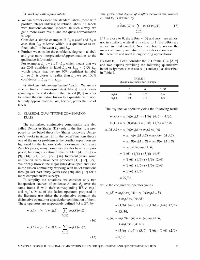
EXAMPLE 1 Let’s consider the 2D frame £ = fA,Bgand two experts providing the following quantitativebelief assignments (masses) m1(¢) and m2(¢) as describedin Table I.

TABLE IQuantitative Inputs for Example 1

A B A[Bm1(¢) 1=6 3=6 2=6m2(¢) 4=6 1=6 1=6

The disjunctive operator yields the following result

m_(A) =m1(A)m2(A) = (1=6) ¢ (4=6) = 4=36,m_(B) =m1(B)m2(B) = (3=6) ¢ (1=6) = 3=36,

m_(A[B) =m1(A)m2(B) +m1(B)m2(A)+m1(A)m2(A[B) +m2(A)m1(A[B)+m1(B)m2(A[B) +m2(B)m1(A[B)+m1(A[B)m2(A[B)

= (1=6) ¢ (1=6)+ (3=6) ¢ (4=6)+ (1=6) ¢ (1=6)+ (4=6) ¢ (2=6)+ (3=6) ¢ (1=6)+ (1=6) ¢ (2=6)+ (2=6) ¢ (1=6)

= 29=36,

while the conjunctive operator yields

m^(A) =m1(A)m2(A) +m1(A)m2(A[B)+m2(A)m1(A[B)

= (1=6) ¢ (4=6)+ (1=6) ¢ (1=6)+ (4=6) ¢ (2=6)= 13=36,

m^(B) =m1(B)m2(B) +m1(B)m2(A[B)+m2(B)m1(A[B)

= (3=6) ¢ (1=6)+ (3=6) ¢ (1=6)+ (1=6) ¢ (2=6)= 8=36,


m^(A[B) =m1(A[B)m2(A[B) = (2=6) ¢ (1=6)=2=36,

m^(A\B)¢=m^(A\B) =m1(A)m2(B)+m2(B)m1(B)

= (1=6) ¢ (1=6)+ (4=6) ¢ (3=6) = 13=36:² Dempster’s rule [3]This combination rule has been initially proposed

by Dempster and then used by Shafer in DST frame-work. We assume (without loss of generality) that thesources of evidence are equally reliable. Otherwise adiscounting preprocessing is first applied. It is definedon G£ = 2£ by forcing mDS(Ø)

¢=0 and 8A 2G£ n fØg

bymDS(A) =

11¡ km^(A) =

m^(A)1¡m^(Ø)

: (19)

When k = 1, this rule cannot be used. Dempster’s ruleof combination can be directly extended for the combi-nation of N independent and equally reliable sources ofevidence and its major interest comes essentially fromits commutativity and associativity properties. Demp-ster’s rule corresponds to the normalized conjunctiverule by reassigning the mass of total conflict onto allfocal elements through the conjunctive operator. Theproblem enlightened by the famous Zadeh’s exam-ple [36] is the repartition of the global conflict. In-deed, consider £ = fA,B,Cg and two experts opinionsgiven by m1(A) = 0:9, m1(C) = 0:1, and m2(B) = 0:9,m2(C) = 0:1, the mass given by Dempster’s combina-tion is mDS(C) = 1 which looks very counter-intuitivesince it reflects the minority opinion. The generalizedZadeh’s example proposed by Smarandache and Dez-ert in [18], shows that the results obtained by Demp-ster’s rule can moreover become totally independent ofthe numerical values taken by m1(¢) and m2(¢) whichis much more surprising and difficult to accept with-out reserve for practical fusion applications. To resolvethis problem, Smets [26] suggested in his TransferableBelief Model (TBM) framework [28] to consider £ asan open-world and therefore to use the conjunctive ruleinstead Dempster’s rule at the credal level. At credallevel m^(Ø) is interpreted as a non-expected solution.The problem is actually just postponed by Smets at thedecision/pignistic level since the normalization (divisionby 1¡m^(Ø)) is also required in order to compute thepignistic probabilities of elements of £. In other words,the non-normalized version of Dempster’s rule corre-sponds to the Smets’ fusion rule in the TBM frame-work working under an open-world assumption, i.e.mS(Ø) = k =m^(Ø) and 8A 2G£ n fØg,mS(A) =m^(A).EXAMPLE 2 Let’s consider the 2D frame and quantita-tive masses as given in example 1 and assume Shafer’smodel (i.e. A\B =Ø), then the conflicting quantitativemass k =m^(A\B) = 13=36 is redistributed to the sets

A, B, A[B proportionally with their m^(¢) masses, i.e.m^(A) = 13=36, m^(B) = 8=36 and m^(A[B) = 2=36respectively through Demspter’s rule (19). One thusgets

mDS(Ø) = 0,

mDS(A) = (13=36)=(1¡ (13=36)) = 13=23,mDS(B) = (8=36)=(1¡ (13=36)) = 8=23,

mDS(A[B) = (2=36)=(1¡ (13=36)) = 2=23:If one prefers to adopt Smets’ TBM approach, at thecredal level the empty set is now allowed to havepositive mass. In this case, one gets

mTBM(Ø) =m^(A\B) = 13=36,mTBM(A) = 13=36,

mTBM(B) = 8=36,

mTBM(A[B) = 2=36:² Yager’s rule [32]—[34]Yager admits that in case of high conflict Dempster’s

rule provides counter-intuitive results. Thus, k plays therole of an absolute discounting term added to the weightof ignorance. The commutative and quasi-associative3

Yager’s rule is given by mY(Ø) = 0 and 8A 2G£ n fØgby

mY(A) =m^(A),

mY(£) =m^(£) +m^(Ø):(20)

EXAMPLE 3 Let’s consider the 2D frame and quantita-tive masses as given in example 1 and assume Shafer’smodel (i.e. A\B =Ø), then the conflicting quantitativemass k =m^(A\B) = 13=36 is transferred to total ig-norance A[B. One thus gets

mY(A) = 13=36,

mY(B) = 8=36,

mY(A[B) = (2=36)+ (13=36) = 15=36:² Dubois & Prade’s rule [5]This rule supposes that the two sources are reliable

when they are not in conflict and at least one of themis right when a conflict occurs. Then if one believesthat a value is in a set X while the other believes thatthis value is in a set Y, the truth lies in X \Y as longX \Y 6=Ø. If X \Y =Ø, then the truth lies in X [Y.According to this principle, the commutative and quasi-associative Dubois & Prade hybrid rule of combination,which is a reasonable trade-off between precision andreliability, is defined by mDP(Ø) = 0 and 8A 2G£ n fØg

3Quasi-associativity was defined by Yager in [34], and Smarandacheand Dezert in [22].


by

mDP(A) =m^(A) +XX,Y2G£X[Y=AX\Y=Ø

m1(X)m2(Y): (21)

In Dubois & Prade’s rule, the conflicting informationis considered more precisely than in Dempster’s orYager’s rules since all partial conflicts involved thetotal conflict are taken into account separately through(21).

The repartition of the conflict is very important be-cause of the non-idempotency of the rules (except theDenœux’ rule [4] that can be applied when the depen-dency between experts is high) and due to the responsesof the experts that can be conflicting. Hence, we havedefined the auto-conflict [16] in order to quantify theintrinsic conflict of a mass and the distribution of theconflict according to the number of experts.

EXAMPLE 4 Taking back example 1 and assumingShafer’s model for £, the quantitative Dubois & Prade’srule gives the same result as quantitative Yager’s rulesince the conflicting mass, m^(A\B) = 13=36, is trans-ferred to A[B, while the other quantitative masses re-main unchanged.

² Proportional Conflict Redistribution (PCR) rulesPCR5 for combining two sourcesSmarandache and Dezert proposed five proportional

conflict redistribution (PCR) methods [21], [22] to re-distribute the partial conflict on the elements impliedin the partial conflict. The most efficient for combiningtwo basic belief assignmentsm1(¢) and m2(¢) is the PCR5rule given by mPCR5(Ø) = 0 and for all X 2G£, X 6=Øby

mPCR5(X)

=m^(X) +XY2G£X\Y´Ø

μm1(X)

2m2(Y)m1(X) +m2(Y)

+m2(X)

2m1(Y)m2(X) +m1(Y)

¶,

(22)

where m^(¢) is the conjunctive rule given by (17).EXAMPLE 5 Let’s consider the 2D frame and quantita-tive masses as given in Example 1 and assume Shafer’smodel (i.e. A\B =Ø), then the conflicting quantitativemass k =m^(A\B) = 13=36 is redistributed only to el-ements involved in conflict, A and B (not to A[B). Werepeat that

m^(A\B) =m1(A)m2(B) +m2(B)m1(B)= (1=6) ¢ (1=6)+ (4=6) ¢ (3=6) = 13=36:

So (1=6) ¢ (1=6) = 1=36 is redistributed to A and Bproportionally to their quantitative masses assignedby the sources (or experts) m1(A) = 1=6 and m2(B)

= 1=6x1,A1=6

=y1,B1=6

=1=36

(1=6)+ (1=6)= 1=12,

hencex1,A = (1=6) ¢ (1=12) = 1=72,

andy1,B = (1=6) ¢ (1=12) = 1=72:

Similarly (4=6) ¢ (3=6) = 12=36 is redistributed to A andB proportionally to their quantitative masses assignedby the sources (or experts) m2(A) = 4=6 and m1(B) =3=6

x2,A4=6

=y2,B3=6

=12=36

(4=6)+ (3=6)= 2=7,

hencex2,A = (4=6) ¢ (2=7) = 4=21,

andy2,B = (3=6) ¢ (2=7) = 1=7:

It is easy to check that

x1,A+ y1,B + x2,A+ y2,B = 13=36 =m^(A\B):Summing, we get

mPCR5(A) = (13=36)+ (1=72)+ (4=21)

= 285=504' 0:57,mPCR5(B) = (8=36)+ (1=72)+ (1=7)

= 191=504' 0:38,mPCR5(A[B) = 2=36' 0:05,

mPCR5(A\B =Ø) = 0:PCR6 for combining more than two sourcesA generalization of PCR5 fusion rule for combining

altogether more than two experts has been proposedby Smarandache and Dezert in [22]. Recently Martinand Osswald [14], [16] studied and formulated a newversion of the PCR5 rule, denoted PCR6, for combiningmore than two sources, say M sources with M ¸ 2.Martin and Osswald have shown that PCR6 exhibits abetter behavior than PCR5 in specific interesting cases.PCR6 rule is defined as follows: mPCR6(Ø) = 0 and forall X 2G£, X 6=Ø,

mPCR6(X) =m^(X) +MXi=1

mi(X)2

XTM¡1k=1

Y¾i (k)\X´Ø

(Y¾i (1),:::,Y¾i (M¡1))2(G

£ )M¡1

¢Ã QM¡1

j=1 m¾i(j)(Y¾

i(j))

mi(X) +PM¡1

j=1 m¾i(j)(Y¾

i(j))

!, (23)

where Yj 2G£ is the response of the expert j, mj(Yj)the associated belief function and ¾i counts from 1 to


M avoiding i

¾i(j) = j if j < i,

¾i(j) = j+1 if j ¸ i:(24)

The idea is here to redistribute the masses of thefocal elements giving a partial conflict proportionallyto the initial masses on these elements.In general, for M ¸ 3 sources, one calculates the

total conflict, which is a sum of products; if eachproduct is formed by factors of masses of distincthypothesis, then PCR6 coincides with PCR5; if atleast a product is formed by at least two factors ofmasses of same hypotheses, then PCR6 is different fromPCR5:² for example: a product like m1(A)m2(A)m3(B), hereinwe have two masses of hypothesis A;

² or m1(A[B)m2(B [C)m3(B [C)m4(B [C), hereinwe have three masses of hypothesis B [C from foursources.

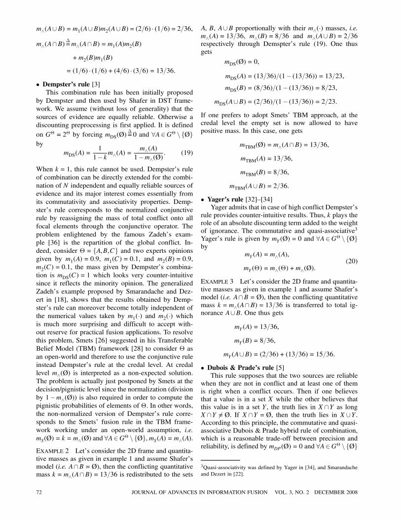
EXAMPLE 6 For instance, consider three expertsexpressing their opinion on £ = fA,B,C,Dg in theShafer’s model as described in Table II.

TABLE IIQuantitative Inputs for Example 6

A B A[C A[B [C [Dm1(¢) 0.7 0 0 0.3m2(¢) 0 0.5 0 0.5m3(¢) 0 0 0.6 0.4

The global conflict is given here by 0:21+0:14+0:09 = 0:44, coming from

–A, B and A[C for the partial conflict 0.21,–A, B and A[B [C [D for 0.14,

–and B, A[C and A[B [C [D for 0.09.With the generalized PCR6 rule (23), we obtain:

mPCR6(A) = 0:14+0:21+0:21 ¢ 718 +0:14 ¢ 716' 0:493,

mPCR6(B) = 0:06+0:21 ¢ 518 +0:14 ¢ 516 + 0:09 ¢ 514' 0:194,

mPCR6(A[C) = 0:09+0:21 ¢ 618 +0:09 ¢ 614 ' 0:199,mPCR6(A[B [C [D) = 0:06+0:14 ¢ 416 +0:09 ¢ 314 ' 0:114:

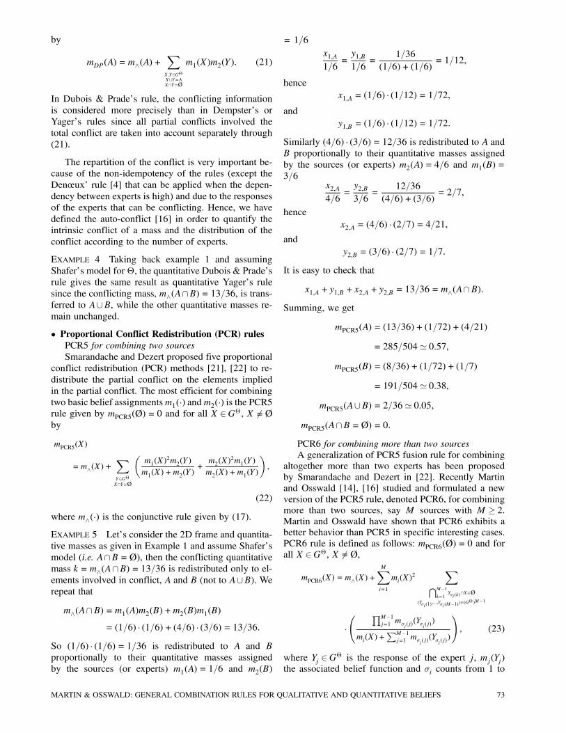
EXAMPLE 7 Let’s consider three sources providingquantitative belief masses only on unions.The conflict is given here by

m^(Ø) =m1(A[B)m2(A[C)m3(B [C)= 0:7 ¢ 0:6 ¢ 0:5 = 0:21:

TABLE IIIQuantitative Inputs for Example 7

A[B B [C A[C A[B [Cm1(¢) 0.7 0 0 0.3m2(¢) 0 0 0.6 0.4m3(¢) 0 0.5 0 0.5

With the generalized PCR rule, i.e. PCR6, we obtain

mPCR6(A) = 0:21,

mPCR6(B) = 0:14,

mPCR6(C) = 0:09,

mPCR6(A[B) = 0:14+0:21: 718 ' 0:2217,

mPCR6(B [C) = 0:06+0:21: 518 ' 0:1183,

mPCR6(A[C) = 0:09+0:21: 618 = 0:16,

mPCR6(A[B [C) = 0:06:In the sequel, we use the notation PCR for two and moresources.

4. CLASSICAL QUALITATIVE COMBINATION RULES

The classical qualitative combination rules are di-rect extensions of classical quantitative rules presentedin previous section. Since the formulas of qualitativefusion rules are the same as for quantitative rules, theywill be not reported in this section. The main differencebetween quantitative and qualitative approaches lies inthe addition, multiplication and division operators onehas to use. For quantitative fusion rules, one uses addi-tion, multiplication and division operators on numberswhile for qualitative fusion rules one uses the addition,multiplication and division operators on linguistic labelsdefined as in Section 2.C1.

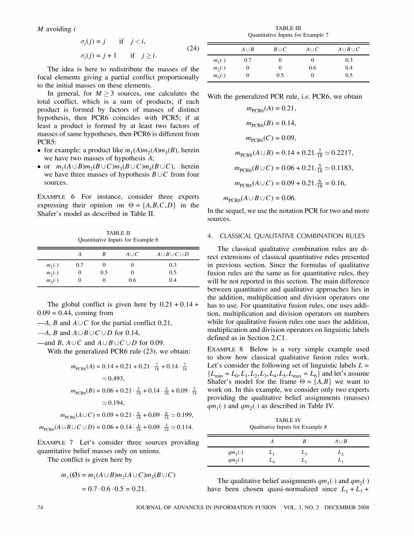
EXAMPLE 8 Below is a very simple example usedto show how classical qualitative fusion rules work.Let’s consider the following set of linguistic labels L=fLmin = L0,L1,L2,L3,L4,L5,Lmax = L6g and let’s assumeShafer’s model for the frame £ = fA,Bg we want towork on. In this example, we consider only two expertsproviding the qualitative belief assignments (masses)qm1(¢) and qm2(¢) as described in Table IV.

TABLE IVQualitative Inputs for Example 8

A B A[Bqm1(¢) L1 L3 L2qm2(¢) L4 L1 L1

The qualitative belief assignments qm1(¢) and qm2(¢)have been chosen quasi-normalized since L1 +L3 +


L2 = L6 = Lmax and respectively L4 +L1 +L1 = L6= Lmax.

² Qualitative Conjunctive rule (QCR)This rule provides qm^(¢) according following

derivations

qm^(A) = qm1(A)qm2(A) + qm1(A)qm2(A[B)+ qm2(A)qm1(A[B)

= L1L4 +L1L1 +L4L2 = L 1¢46+L 1¢1

6+L 4¢2

6

= L 4+1+86= L 13

6,

qm^(B) = qm1(B)qm2(B) +qm1(B)qm2(A[B)+ qm2(B)qm1(A[B)

= L3L1 +L3L1 +L1L2 = L 3¢16+L 3¢1

6+L 1¢2

6

= L 3+3+26= L 8

6,

qm^(A[B) = qm1(A[B)qm2(A[B) = L2L1 = L 2¢16

= L 26,

qm^(A\B) = qm1(A)qm2(B) +qm2(B)qm1(B)= L1L1 +L4L3 = L 1¢1

6+L 4¢3

6= L 1+12

6= L 13

6:

We see that not approximating the indexes (i.e. work-ing with refined labels), the quasi-normalization of thequalitative conjunctive rule is kept

L 136+L 8

6+L 2

6+L 13

6= L 36

6= L6 = Lmax:

But if we approximate each refined label, we get

L[ 136 ]+L[ 86 ] +L[ 26 ] +L[ 136 ]

= L2 +L1 +L0 +L2 = L5 6= L6 = Lmax:

Let’s examine the transfer of the conflicting qualita-tive mass qm^(A\B) = qm^(Ø) = L 13

6to the non-empty

sets according to the main following combinationrules.

² Qualitative Dempster’s rule (extension of classicalnumerical DS rule to qualitative masses)Assuming Shafer’s model for the frame £ (i.e.

A\B =Ø) and according to DS rule, the conflictingqualitative mass qm^(A\B) = L 13

6is redistributed to the

sets A, B, A[B proportionally with their qm^(¢) massesL 13

6, L 8

6, and L 2

6respectively,

xAL 13

6

=yBL 86

=zA[BL 26

=L 13

6

L 136+L 8

6+L 2

6

=L 13

6

L 236

= L( 136 ¥ 236 )¢6 = L( 1323 )¢6 = L 78

23:

Therefore, one gets

xA = L 136¢L 78

23= L( 136 ¢ 7823 )¥6 = L 169

138,

yB = L 86¢L 78

23= L( 86 ¢ 7823 )¥6 = L 104

138,

zA[B = L 26¢L 78

23= L( 26 ¢ 7823 )¥6 = L 26

138:

We can check that the qualitative conflicting mass,L 13

6, has been proportionally split into three qualitative

masses

L 169138+L 104

138+L 26

138= L 169+104+26

138= L 299

138= L 13

6:

Thus,

qmDS(A) = L 136+L 169

138= L 13

6 +169138= L 468

138,

qmDS(B) = L 86+L 104

138= L 8

6+104138= L 288

138,

qmDS(A[B) = L 26+L 26

138= L 2

6 +26138= L 72

138,

qmDS(A\B =Ø) = L0:qmDS(¢) is quasi-normalized since:

L 468138+L 288

138+L 72

138= L 828

138= L6 = Lmax:

If we approximate the linguistic labels L 468138, L 288

138and

L 72138in order to work with original labels in L, still

qmDS(¢) remains quasi-normalized since:qmDS(A)¼ L[ 468138 ] = L3qmDS(B)¼ L[ 288138 ] = L2

qmDS(A[B)¼ L[ 72138 ] = L1and L3 +L2 +L1 = L6 = Lmax.

² Qualitative Yager’s ruleWith Yager’s rule, the qualitative conflicting mass

L 136is entirely transferred to the total ignorance A[B.

Thus,qmY(A[B) = L 2

6+L 13

6= L 15

6

andqmY(A\B) = qmY(Ø) = L0

while the others remain the same

qmY(A) = L 136,

qmY(B) = L 86:

qmY(¢) is quasi-normalized sinceL 13

6+L 8

6+L 15

6= L 36

6= L6 = Lmax:

If we approximate the linguistic labels L 136, L 8

6and L 15

6,

still qmY(¢) happens to remain quasi-normalized sinceqmY(A)¼ L[ 136 ] = L2,qmY(B)¼ L[ 86 ] = L1,

qmY(A[B)¼ L[ 156 ] = L3,and L2 +L1 +L3 = L6 = Lmax.


² Qualitative Dubois & Prade’s ruleIn this example the Qualitative Dubois & Prade’s

rule gives the same result as qualitative Yager’s rulesince the conflicting mass, qm^(A\B) = L 13

6, is trans-

ferred to A[B, while the other qualitative masses re-main unchanged.

² Qualitative Smets’ TBM ruleSmets’ TBM approach allows keeping mass on the

empty set. One gets

qmTBM(A) = L 136,

qmTBM(B) = L 86,

qmTBM(A[B) = L 26,

qmTBM(Ø) = L 136:

Of course qmTBM(¢) is also quasi-normalized.However if we approximate, qmTBM(¢) does not re-

main quasi-normalized in this case since

qmTBM(A)¼ L[ 136 ] = L2,

qmTBM(B)¼ L[ 86 ] = L1,

qmTBM(A[B)¼ L[ 26 ] = L0,

qmTBM(Ø)¼ L[ 136 ] = L2,and L2 +L1 +L0 +L2 = L5 6= L6 = Lmax.² Qualitative PCR (QPCR)The conflicting qualitative mass, qm^(A\B) = L 13

6,

is redistributed only to elements involved in conflict, Aand B (not to A[B). We repeat thatqmPCR(A\B) = qm1(A)qm2(B)+ qm2(B)qm1(B)

= L1L1 +L4L3 = L 1¢16+L 4¢3

6= L 1+12

6= L 13

6:

So L 16is redistributed to A and B proportionally to their

qualitative masses assigned by the sources (or experts)qm1(A) = L1 and qm2(B) = L1

x1,AL1

=y1,BL1

=L 16

L1 +L1=L 16

L2= L( 16¥2)¢6 = L 1

2:

Hencex1,A = L1 ¢L 1

2= L(1¢ 12 )¥6 = L 1

12

andy1,B = L1 ¢L 1

2= L 1

12:

Similarly L 126is redistributed to A and B proportionally

to their qualitative masses assigned by the sources (orexperts) qm2(A) = L4 and qm1(B) = L3

x2,AL4

=y2,BL3

=L 12

6

L4 +L3=L 12

6

L7= L( 126 ¥7)¢6 = L 12

7:

Hencex2,A = L4 ¢L 12

7= L(4¢ 127 )¥6 = L 8

7

andy2,B = L3 ¢L 12

7= L(3¢ 127 )¥6 = L 6

7:

Summing, we get

qmPCR(A) = L 136+L 1

12+L 8

7= L 285

84,

qmPCR(B) = L 86+L 1

12+L 6

7= L 191

84,

qmPCR(A[B) = L 26= L 28

84,

qmPCR(A\B =Ø) = L0:qmPCR(¢) is quasi-normalized since

L 28584+L 191

84+L 28

84= L 504

84= L6 = Lmax:

However, if we approximate, it is not quasi-normalizedany longer since

L[ 28584 ]+L[ 19184 ] +L[ 2884 ] = L3 +L2 +L0 = L5 6= L6 = Lmax:

In general, if we do not approximate, and we workwith quasi-normalized qualitative masses, no matterwhat fusion rule we apply, the result will be quasi-normalized. If we approximate, many times the quasi-normalization is lost.

5. GENERALIZATION OF QUANTITATIVE FUSIONRULES

In [1], [29] we can find two propositions of ageneral formulation of the combination rules. In thefirst one, Smets considers the combination rules froma matrix notation and find the shape of this matrixaccording to some assumptions on the rule, such aslinearity, commutativity, associativity, etc. In the secondone, a generic operator is defined from the plausibilityfunctions.A general formulation of the global conflict repar-

tition have been proposed in [8], [12] for all X 2 2£by

mc(X) =m^(X) +w(X)m^(Ø), (25)

wherePX22£ w(X) = 1. The problem is the choice of

the weights w(X).

A. How to Choose Conjunctive and Disjunctive Rules?

We have seen that conjunctive rule reduces the im-precision and uncertainty but can be used only if one ofthe experts is reliable, whereas the disjunctive rule canbe used when the experts are not reliable, but allows aloss of specificity.Hence, Florea [7] proposes a weighted sum of these

two rules according to the global conflict k =m^(Ø)


given for X 2 2£ by:mFlo(X) = ¯1(k)m_(X) +¯2(k)m^(X), (26)

where ¯1 and ¯2 can admit k =12 as symmetric weight:

¯1(k) =k

1¡ k+ k2 ,

¯2(k) =1¡ k

1¡ k+ k2 :(27)

Consequently, if the global conflict is high (k near 1)the behavior of this rule will give more importanceto the disjunctive rule. Thus, this rule considers theglobal conflict coming from the non-reliability of theexperts.In order to take into account the weights more

precisely in each partial combination, we propose thefollowing new rule. For two basic belief assignmentsm1 and m2 and for all X 2G£, X 6=Ø we have:

mMix(X) =X

Y1[Y2=X±1(Y1,Y2)m1(Y1)m2(Y2)

+X

Y1\Y2=X±2(Y1,Y2)m1(Y1)m2(Y2): (28)

Of course, if ±1(Y1,Y2) = ¯1(k) and ±2(Y1,Y2) = ¯2(k)we obtain Florea’s rule. In the same manner, if ±1(Y1,Y2)= 1¡ ±2(Y1,Y2) = 0 we obtain the conjunctive rule andif ±1(Y1,Y2) = 1¡ ±2(Y1,Y2) = 1 the disjunctive rule. If±1(Y1,Y2) = 1¡ ±2(Y1,Y2) = 1lY1\Y2=Ø we retrieve Duboisand Prade’s rule and the partial conflict can be con-sidered, whereas the rule (26).The choice of ±1(Y1,Y2) = 1¡ ±2(Y1,Y2) can be done

by a dissimilarity such as:

±1(Y1,Y2) = ±(Y1,Y2)¢=1¡ C(Y1 \Y2)

minfC(Y1),C(Y2)g,

(29)or

±1(Y1,Y2) = ´(Y1,Y2)¢=1¡ C(Y1 \Y2)

maxfC(Y1),C(Y2)g,

(30)

where C(Y1) is the cardinality of Y1. In the case ofthe DST framework, C(Y1) is the number of distinctelements of Y1. In the case of the DSmT, C(Y1) is theDSm cardinality given by the number of parts of Y1in the Venn diagram of the problem [18]. ±(¢, ¢) in(29) is actually not a proper dissimilarity measure (e.g.±(Y1,Y2) = 0 does not imply Y1 = Y2), but ´(¢, ¢) definedin (30) is a proper dissimilarity measure. We can alsotake for ±2(Y1,Y2), the Jaccard’s distance, i.e. ±2(Y1,Y2) =d(Y1,Y2) given by

d(Y1,Y2) =C(Y1 \Y2)C(Y1 [Y2)

, (31)

used by [10] on the belief functions. Note that d is nota distance in the case of DSmT. Thus, if we have a

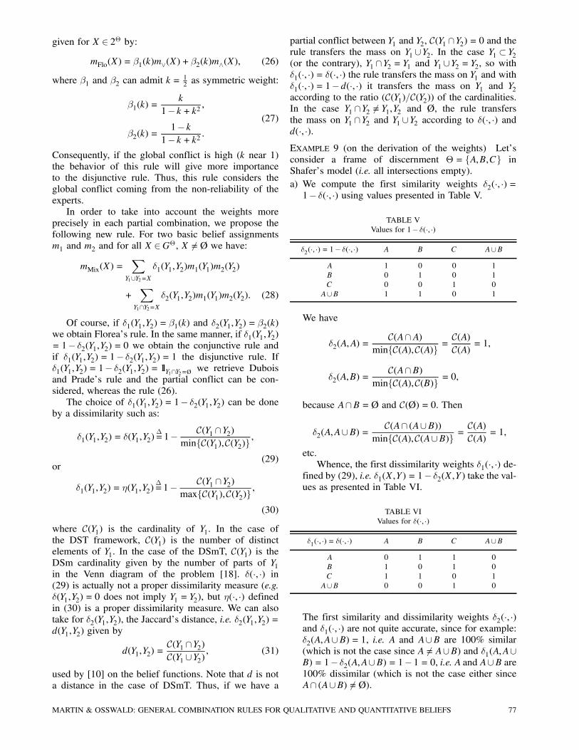
partial conflict between Y1 and Y2, C(Y1 \Y2) = 0 and therule transfers the mass on Y1 [Y2. In the case Y1 ½ Y2(or the contrary), Y1 \Y2 = Y1 and Y1 [Y2 = Y2, so with±1(¢, ¢) = ±(¢, ¢) the rule transfers the mass on Y1 and with±1(¢, ¢) = 1¡ d(¢, ¢) it transfers the mass on Y1 and Y2according to the ratio (C(Y1)=C(Y2)) of the cardinalities.In the case Y1 \Y2 6= Y1,Y2 and Ø, the rule transfersthe mass on Y1 \Y2 and Y1 [Y2 according to ±(¢, ¢) andd(¢, ¢).EXAMPLE 9 (on the derivation of the weights) Let’sconsider a frame of discernment £ = fA,B,Cg inShafer’s model (i.e. all intersections empty).a) We compute the first similarity weights ±2(¢, ¢) =1¡ ±(¢, ¢) using values presented in Table V.

TABLE VValues for 1¡ ±(¢, ¢)

±2(¢, ¢) = 1¡ ±(¢, ¢) A B C A[BA 1 0 0 1B 0 1 0 1C 0 0 1 0

A[B 1 1 0 1

We have

±2(A,A) =C(A\A)

minfC(A),C(A)g =C(A)C(A) = 1,

±2(A,B) =C(A\B)

minfC(A),C(B)g = 0,

because A\B =Ø and C(Ø) = 0. Then

±2(A,A[B) =C(A\ (A[B))

minfC(A),C(A[B)g =C(A)C(A) = 1,

etc.Whence, the first dissimilarity weights ±1(¢, ¢) de-

fined by (29), i.e. ±1(X,Y) = 1¡ ±2(X,Y) take the val-ues as presented in Table VI.

TABLE VIValues for ±(¢, ¢)

±1(¢, ¢) = ±(¢, ¢) A B C A[BA 0 1 1 0B 1 0 1 0C 1 1 0 1

A[B 0 0 1 0

The first similarity and dissimilarity weights ±2(¢, ¢)and ±1(¢, ¢) are not quite accurate, since for example:±2(A,A[B) = 1, i.e. A and A[B are 100% similar(which is not the case since A 6= A[B) and ±1(A,A[B) = 1¡ ±2(A,A[B) = 1¡ 1 = 0, i.e. A and A[B are100% dissimilar (which is not the case either sinceA\ (A[B) 6=Ø).


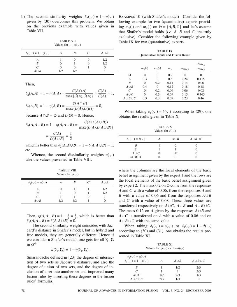
b) The second similarity weights ±2(¢, ¢) = 1¡ ´(¢, ¢)given by (30) overcomes this problem. We obtainon the previous example with values given inTable VII.

TABLE VIIValues for 1¡ ´(¢, ¢)

±2(¢, ¢) = 1¡ ´(¢, ¢) A B C A[BA 1 0 0 1/2B 0 1 0 1/2C 0 0 1 0

A[B 1/2 1/2 0 1

Then,

±2(A,A) = 1¡ ´(A,A) =C(A\A)

maxfC(A),C(A)g =C(A)C(A) = 1,

±2(A,B) = 1¡ ´(A,B) =C(A\B)

maxfC(A),C(B)g = 0,

because A\B =Ø and C(Ø) = 0. Hence,

±2(A,A[B) = 1¡ ´(A,A[B) =C(A\ (A[B))

maxfC(A),C(A[B)g

=C(A)

C(A[B) =12

which is better than ±2(A,A[B) = 1¡ ±(A,A[B) = 1.etc.Whence, the second dissimilarity weights ´(¢, ¢)

take the values presented in Table VIII.

TABLE VIIIValues for ´(¢, ¢)

±1(¢, ¢) = ´(¢, ¢) A B C A[BA 0 1 1 1/2B 1 0 1 1/2C 1 1 0 1

A[B 1/2 1/2 1 0

Then, ´(A,A[B) = 1¡ 12 =

12 , which is better than

±1(A,A[B) = ±(A,A[B) = 0.The second similarity weight coincides with Jac-

card’s distance in Shafer’s model, but in hybrid andfree models, they are generally different. Hence ifwe consider a Shafer’s model, one gets for all Y1, Y2in G£

d(Y1,Y2) = 1¡ ´(Y1,Y2):Smarandache defined in [23] the degree of intersec-tion of two sets as Jaccard’s distance, and also thedegree of union of two sets, and the degree of in-clusion of a set into another set and improved manyfusion rules by inserting these degrees in the fusionrules’ formulas.

EXAMPLE 10 (with Shafer’s model) Consider the fol-lowing example for two (quantitative) experts provid-ing m1(¢) and m2(¢) on £ = fA,B,Cg and let’s assumethat Shafer’s model holds (i.e. A, B and C are trulyexclusive). Consider the following example given byTable IX for two (quantitative) experts.

TABLE IXQuantitative Inputs and Fusion Result

mMix,´m1(¢) m2(¢) m^ mMix,± mMix,d

Ø 0 0 0.2 0 0A 0.3 0 0.3 0.24 0.115B 0 0.2 0.14 0.14 0.06

A[B 0.4 0 0.12 0.18 0.18C 0 0.2 0.06 0.06 0.02

A[C 0 0.3 0.09 0.15 0.165A[B [C 0.3 0.3 0.09 0.23 0.46

When taking ±1(¢, ¢) = ±(¢, ¢) according to (29), oneobtains the results given in Table X.

TABLE XValues for ±(¢, ¢)

±1(¢, ¢) = ±(¢, ¢) A A[B A[B [CB 1 0 0C 1 1 0

A[C 0 1/2 0A[B [C 0 0 0

where the columns are the focal elements of the basicbelief assignment given by the expert 1 and the rows arethe focal elements of the basic belief assignment givenby expert 2. The mass 0.2 on Ø come from the responsesA and C with a value of 0.06, from the responses A andB with a value of 0.06 and from the responses A[Band C with a value of 0.08. These three values aretransferred respectively on A[C, A[B and A[B [C.The mass 0.12 on A given by the responses A[B andA[C is transferred on A with a value of 0.06 and onA[B [C with the same value.When taking ±1(¢, ¢) = ´(¢, ¢) or ±1(¢, ¢) = 1¡ d(¢, ¢)

according to (30) and (31), one obtains the results pre-sented in Table XI.

TABLE XIValues for ´(¢, ¢) or 1¡ d(¢, ¢)

±1(¢, ¢) = ´(¢, ¢)±1(¢, ¢) = 1¡ d(¢, ¢) A A[B A[B [C

B 1 1/2 2/3C 1 1 2/3

A[C 1/2 2/3 1/3A[B [C 2/3 1/3 0


With ±1(¢, ¢) = ´ or ±1(¢, ¢) = 1¡ d(¢, ¢), the rule is moredisjunctive: more masses are transferred on the igno-rance.Note that ±1(¢, ¢) = ±(¢, ¢) can be used when the ex-

perts are considered reliable. In this case, we con-sider the most precise response. With ±1(¢, ¢) = ´(¢, ¢)or ±1(¢, ¢) = 1¡ d(¢, ¢), we get the conjunctive rule onlywhen the experts provide the same response, otherwisewe consider the doubtful responses and we transfer themasses in proportion of the imprecision of the responses(given by the cardinality of the responses) on the partin agreement and on the partial ignorance.

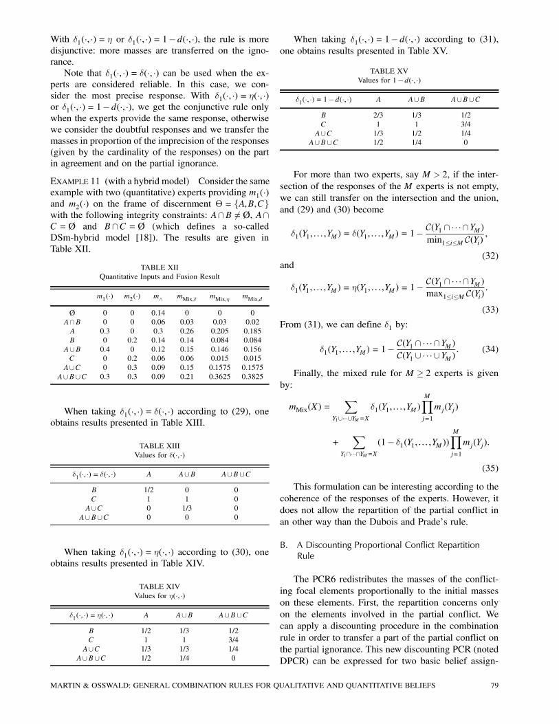
EXAMPLE 11 (with a hybrid model) Consider the sameexample with two (quantitative) experts providing m1(¢)and m2(¢) on the frame of discernment £ = fA,B,Cgwith the following integrity constraints: A\B 6=Ø, A\C =Ø and B \C =Ø (which defines a so-calledDSm-hybrid model [18]). The results are given inTable XII.

TABLE XIIQuantitative Inputs and Fusion Result

m1(¢) m2(¢) m^ mMix,± mMix,´ mMix,d

Ø 0 0 0.14 0 0 0A\B 0 0 0.06 0.03 0.03 0.02A 0.3 0 0.3 0.26 0.205 0.185B 0 0.2 0.14 0.14 0.084 0.084

A[B 0.4 0 0.12 0.15 0.146 0.156C 0 0.2 0.06 0.06 0.015 0.015

A[C 0 0.3 0.09 0.15 0.1575 0.1575A[B [C 0.3 0.3 0.09 0.21 0.3625 0.3825

When taking ±1(¢, ¢) = ±(¢, ¢) according to (29), oneobtains results presented in Table XIII.

TABLE XIIIValues for ±(¢, ¢)

±1(¢, ¢) = ±(¢, ¢) A A[B A[B [CB 1/2 0 0C 1 1 0

A[C 0 1/3 0A[B [C 0 0 0

When taking ±1(¢, ¢) = ´(¢, ¢) according to (30), oneobtains results presented in Table XIV.

TABLE XIVValues for ´(¢, ¢)

±1(¢, ¢) = ´(¢, ¢) A A[B A[B [CB 1/2 1/3 1/2C 1 1 3/4

A[C 1/3 1/3 1/4A[B [C 1/2 1/4 0

When taking ±1(¢, ¢) = 1¡ d(¢, ¢) according to (31),one obtains results presented in Table XV.

TABLE XVValues for 1¡ d(¢, ¢)

±1(¢, ¢) = 1¡ d(¢, ¢) A A[B A[B [CB 2/3 1/3 1/2C 1 1 3/4

A[C 1/3 1/2 1/4A[B [C 1/2 1/4 0

For more than two experts, say M > 2, if the inter-section of the responses of the M experts is not empty,we can still transfer on the intersection and the union,and (29) and (30) become

±1(Y1, : : : ,YM) = ±(Y1, : : : ,YM) = 1¡C(Y1 \ ¢¢ ¢ \YM)min1·i·M C(Yi)

,

(32)and

±1(Y1, : : : ,YM) = ´(Y1, : : : ,YM) = 1¡C(Y1 \ ¢ ¢ ¢ \YM)max1·i·M C(Yi)

:

(33)

From (31), we can define ±1 by:

±1(Y1, : : : ,YM) = 1¡C(Y1 \ ¢ ¢ ¢ \YM)C(Y1 [ ¢ ¢ ¢ [YM)

: (34)

Finally, the mixed rule for M ¸ 2 experts is givenby:

mMix(X) =X

Y1[¢¢¢[YM=X±1(Y1, : : : ,YM)

MYj=1

mj(Yj)

+X

Y1\¢¢¢\YM=X(1¡ ±1(Y1, : : : ,YM))

MYj=1

mj(Yj):

(35)

This formulation can be interesting according to thecoherence of the responses of the experts. However, itdoes not allow the repartition of the partial conflict inan other way than the Dubois and Prade’s rule.

B. A Discounting Proportional Conflict RepartitionRule

The PCR6 redistributes the masses of the conflict-ing focal elements proportionally to the initial masseson these elements. First, the repartition concerns onlyon the elements involved in the partial conflict. Wecan apply a discounting procedure in the combinationrule in order to transfer a part of the partial conflict onthe partial ignorance. This new discounting PCR (notedDPCR) can be expressed for two basic belief assign-


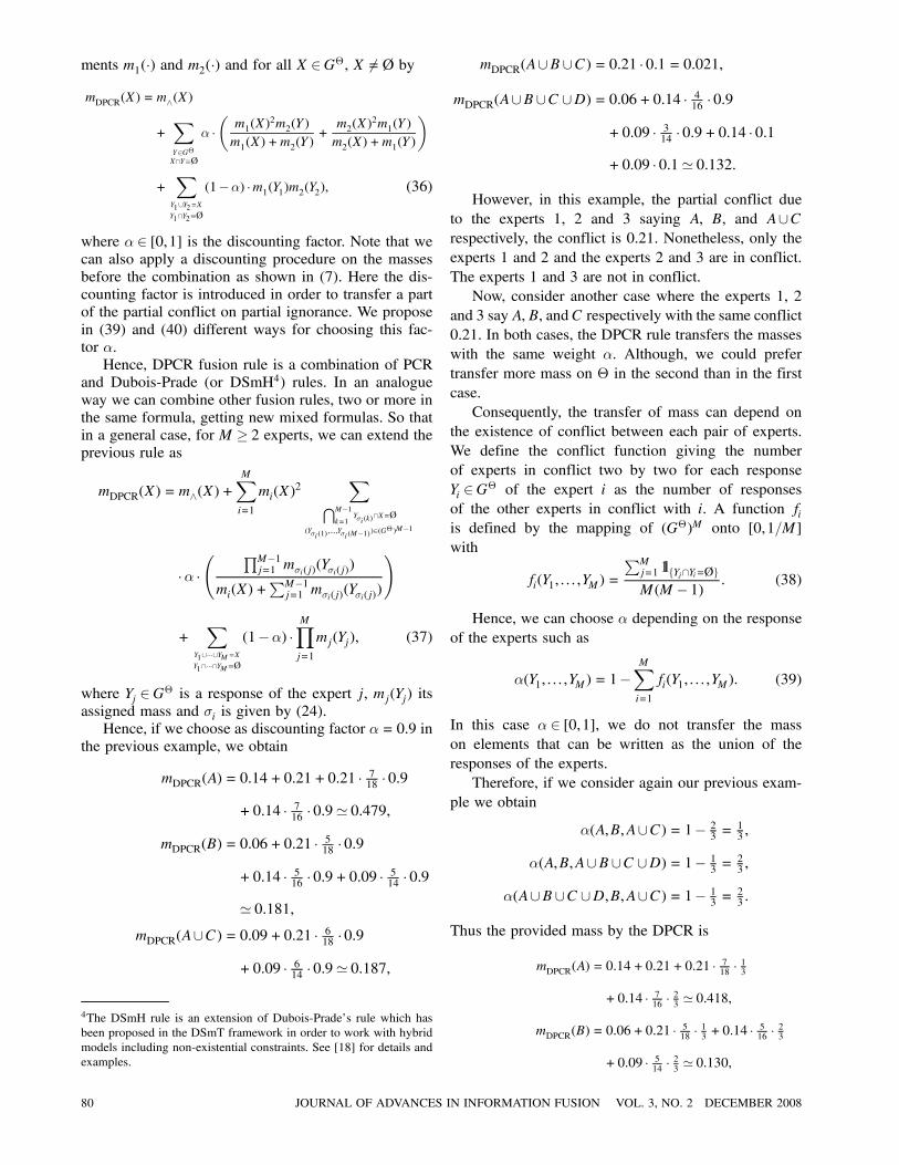
ments m1(¢) and m2(¢) and for all X 2G£, X 6=Ø bymDPCR(X) =m^(X)

+XY2G£X\Y´Ø

® ¢μm1(X)

2m2(Y)m1(X) +m2(Y)

+m2(X)

2m1(Y)m2(X) +m1(Y)

¶

+XY1[Y2=XY1\Y2´Ø

(1¡®) ¢m1(Y1)m2(Y2), (36)

where ® 2 [0,1] is the discounting factor. Note that wecan also apply a discounting procedure on the massesbefore the combination as shown in (7). Here the dis-counting factor is introduced in order to transfer a partof the partial conflict on partial ignorance. We proposein (39) and (40) different ways for choosing this fac-tor ®.Hence, DPCR fusion rule is a combination of PCR

and Dubois-Prade (or DSmH4) rules. In an analogueway we can combine other fusion rules, two or more inthe same formula, getting new mixed formulas. So thatin a general case, for M ¸ 2 experts, we can extend theprevious rule as

mDPCR(X) =m^(X) +MXi=1

mi(X)2

XTM¡1k=1

Y¾i (k)\X=Ø

(Y¾i (1),:::,Y¾i (M¡1))2(G

£ )M¡1

¢® ¢Ã QM¡1

j=1 m¾i(j)(Y¾i(j))

mi(X) +PM¡1

j=1 m¾i(j)(Y¾i(j))

!

+X

Y1[¢¢¢[YM=XY1\¢¢¢\YM´Ø

(1¡®) ¢MYj=1

mj(Yj), (37)

where Yj 2G£ is a response of the expert j, mj(Yj) itsassigned mass and ¾i is given by (24).Hence, if we choose as discounting factor ®= 0:9 in

the previous example, we obtain

mDPCR(A) = 0:14+0:21+0:21 ¢ 718 ¢ 0:9

+0:14 ¢ 716 ¢ 0:9' 0:479,

mDPCR(B) = 0:06+0:21 ¢ 518 ¢0:9

+0:14 ¢ 516 ¢ 0:9+0:09 ¢ 514 ¢ 0:9

' 0:181,mDPCR(A[C) = 0:09+0:21 ¢ 618 ¢0:9

+0:09 ¢ 614 ¢ 0:9' 0:187,

4The DSmH rule is an extension of Dubois-Prade’s rule which hasbeen proposed in the DSmT framework in order to work with hybridmodels including non-existential constraints. See [18] for details andexamples.

mDPCR(A[B [C) = 0:21 ¢ 0:1 = 0:021,

mDPCR(A[B [C [D) = 0:06+0:14 ¢ 416 ¢ 0:9

+0:09 ¢ 314 ¢ 0:9+0:14 ¢ 0:1

+0:09 ¢ 0:1' 0:132:

However, in this example, the partial conflict dueto the experts 1, 2 and 3 saying A, B, and A[Crespectively, the conflict is 0.21. Nonetheless, only theexperts 1 and 2 and the experts 2 and 3 are in conflict.The experts 1 and 3 are not in conflict.Now, consider another case where the experts 1, 2

and 3 say A, B, and C respectively with the same conflict0.21. In both cases, the DPCR rule transfers the masseswith the same weight ®. Although, we could prefertransfer more mass on £ in the second than in the firstcase.Consequently, the transfer of mass can depend on

the existence of conflict between each pair of experts.We define the conflict function giving the numberof experts in conflict two by two for each responseYi 2G£ of the expert i as the number of responsesof the other experts in conflict with i. A function fiis defined by the mapping of (G£)M onto [0,1=M]with

fi(Y1, : : : ,YM) =

PMj=1 1lfYj\Yi=ØgM(M ¡ 1) : (38)

Hence, we can choose ® depending on the responseof the experts such as

®(Y1, : : : ,YM) = 1¡MXi=1

fi(Y1, : : : ,YM): (39)

In this case ® 2 [0,1], we do not transfer the masson elements that can be written as the union of theresponses of the experts.Therefore, if we consider again our previous exam-

ple we obtain

®(A,B,A[C) = 1¡ 23 =

13 ,

®(A,B,A[B [C [D) = 1¡ 13 =

23 ,

®(A[B [C [D,B,A[C) = 1¡ 13 =

23 :

Thus the provided mass by the DPCR is

mDPCR(A) = 0:14+0:21+0:21 ¢ 718 ¢ 13+0:14 ¢ 716 ¢ 23 ' 0:418,

mDPCR(B) = 0:06+0:21 ¢ 518 ¢ 13 +0:14 ¢ 516 ¢ 23+0:09 ¢ 514 ¢ 23 ' 0:130,


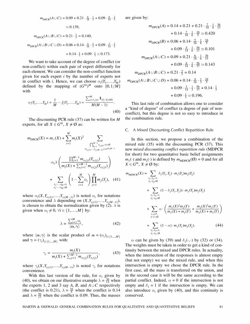
mDPCR(A[C) = 0:09+0:21 ¢ 618 ¢ 13 + 0:09 ¢ 614 ¢ 23' 0:139,

mDPCR(A[B [C) = 0:21 ¢ 23 = 0:140,

mDPCR(A[B [C [D) = 0:06+0:14 ¢ 416 ¢ 23 + 0:09 ¢ 314 ¢ 23+0:14 ¢ 13 +0:09 ¢ 13 ' 0:173:

We want to take account of the degree of conflict (ornon-conflict) within each pair of expert differently foreach element. We can consider the non-conflict functiongiven for each expert i by the number of experts notin conflict with i. Hence, we can choose ®i(Y1, : : : ,YM)defined by the mapping of (G£)M onto [0,1=M]with

®i(Y1, : : : ,YM) =1M¡fi(Y1, : : : ,YM) =

PM

j=1,j 6=i 1lfYj\Yi 6´Øg

M(M ¡ 1) :

(40)

The discounting PCR rule (37) can be written for Mexperts, for all X 2G£, X 6=Ø as:

mDPCR(X) =m^(X) +MXi=1

mi(X)2

XTM¡1k=1

Y¾i (k)\X=Ø

(Y¾i (1),:::,Y¾i (M¡1))2(G

£ )M¡1

¢®i¸Ã QM¡1

j=1 m¾i(j)(Y¾i(j))

mi(X) +PM¡1j=1 m¾i(j)(Y¾i(j))

!

+X

Y1[¢¢¢[YM=XY1\¢¢¢\YM´Ø

Ã1¡

MXi=1

®i

!MYj=1

mj(Yj), (41)

where ®i(X,Y¾i(1), : : : ,Y¾i(M¡1)) is noted ®i for notationsconvenience and ¸ depending on (X,Y¾i(1), : : : ,Y¾i(M¡1)),is chosen to obtain the normalization given by (2). ¸ isgiven when ®i 6= 0, 8i 2 f1, : : : ,Mg by:

¸=PMi=1®ih®,°i , (42)

where h®,°i is the scalar product of ®= (®i)i2f1,:::,Mgand ° = (°i)i2f1,:::,Mg with:

°i =mi(X)

mi(X)+PM¡1j=1 m¾i(j)(Y¾i(j))

, (43)

where °i(X,Y¾i(1), : : : ,Y¾i(M¡1)) is noted °i for notationsconvenience.With this last version of the rule, for ®i given by

(40), we obtain on our illustrative example ¸= 3613 when

the experts 1, 2 and 3 say A, B, and A[C respectively(the conflict is 0.21), ¸= 16

5 when the conflict is 0.14and ¸= 56

17 when the conflict is 0.09. Thus, the masses

are given by:

mDPCR(A) = 0:14+0:21+0:21 ¢ 718 ¢ 16 ¢ 3613+0:14 ¢ 716 ¢ 16 ¢ 165 ' 0:420

mDPCR(B) = 0:06+0:14 ¢ 516 ¢ 16 ¢ 165+0:09 ¢ 514 ¢ 16 ¢ 5617 ' 0:101

mDPCR(A[C) = 0:09+0:21 ¢ 618 ¢ 16 ¢ 3613+0:09 ¢ 614 ¢ 16 ¢ 5617 ' 0:143

mDPCR(A[B [C) = 0:21 ¢ 23 = 0:14mDPCR(A[B [C [D) = 0:06+0:14 ¢ 416 ¢ 13 ¢ 165

+0:09 ¢ 314 ¢ 13 ¢ 5617 +0:14 ¢ 13+0:09 ¢ 13 ' 0:196:

This last rule of combination allows one to considera “kind of degree” of conflict (a degree of pair of non-conflict), but this degree is not so easy to introduce inthe combination rule.

C. A Mixed Discounting Conflict Repartition Rule

In this section, we propose a combination of themixed rule (35) with the discounting PCR (37). Thisnew mixed discounting conflict repartition rule (MDPCRfor short) for two quantitative basic belief assignmentsm1(¢) and m2(¢) is defined by mMDPCR(Ø) = 0 and for allX 2G£, X 6=Ø by:mMDPCR(X) =

XY1[Y2=X,Y1\Y2 6´Ø

±1(Y1,Y2) ¢m1(Y1)m2(Y2)

+X

Y1\Y2=X,Y1\Y2 6´Ø

(1¡ ±1(Y1,Y2)) ¢m1(Y1)m2(Y2)

+XY2G£ ,X\Y´Ø

® ¢μm1(X)

2m2(Y)m1(X) +m2(Y)

+m2(X)

2m1(Y)m2(X) +m1(Y)

¶

+X

Y1[Y2=X,Y1\Y2´Ø

(1¡®) ¢m1(Y1)m2(Y2): (44)

® can be given by (39) and ±1(¢, ¢) by (32) or (34).The weights must be taken in order to get a kind of con-tinuity between the mixed and DPCR rules. In actuality,when the intersection of the responses is almost empty(but not empty) we use the mixed rule, and when thisintersection is empty we chose the DPCR rule. In thefirst case, all the mass is transferred on the union, andin the second case it will be the same according to thepartial conflict. Indeed, ®= 0 if the intersection is notempty and ±1 = 1 if the intersection is empty. We canalso introduce ®i given by (40), and this continuity isconserved.


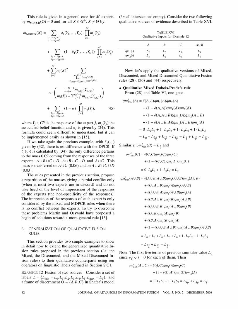
This rule is given in a general case for M experts,by mMDPCR(Ø) = 0 and for all X 2G£, X 6=Ø by:

mMDPCR(X) =X

Y1[¢¢¢[YM=X ,Y1\¢¢¢\YM 6´Ø

±1(Y1, : : : ,YM) ¢MYj=1

mj(Yj)

+X

Y1\¢¢¢\YM=X,Y1\¢¢¢\YM 6´Ø

(1¡ ±1(Y1, : : : ,YM)) ¢MYj=1

mj(Yj)

+MXi=1

mi(X)2

XTM¡1k=1

Y¾i (k)\X=Ø

(Y¾i (1),:::,Y¾i (M¡1))2(G

£ )M¡1

¢® ¢Ã QM¡1

j=1 m¾i(j)(Y¾i(j))

mi(X) +PM¡1

j=1 m¾i(j)(Y¾i(j))

!

+X

Y1[¢¢¢[YM=X,Y1\¢¢¢\YM´Ø

(1¡®) ¢MYj=1

mj(Yj), (45)

where Yj 2G£ is the response of the expert j, mj(Yj) theassociated belief function and ¾i is given by (24). Thisformula could seem difficult to understand, but it canbe implemented easily as shown in [15].If we take again the previous example, with ±1(¢, ¢)

given by (32), there is no difference with the DPCR. If±1(¢, ¢) is calculated by (34), the only difference pertainsto the mass 0.09 coming from the responses of the threeexperts: A[B [C [D, A[B [C [D and A[C. Thismass is transferred on A[C (0.06) and on A[B [C [D(0.03).The rules presented in the previous section, propose

a repartition of the masses giving a partial conflict only(when at most two experts are in discord) and do nottake heed of the level of imprecision of the responsesof the experts (the non-specificity of the responses).The imprecision of the responses of each expert is onlyconsidered by the mixed and MDPCR rules when thereis no conflict between the experts. To try to overcomethese problems Martin and Osswald have proposed abegin of solutions toward a more general rule [15].

6. GENERALIZATION OF QUALITATIVE FUSIONRULES

This section provides two simple examples to showin detail how to extend the generalized quantitative fu-sion rules proposed in the previous section (i.e. theMixed, the Discounted, and the Mixed Discounted fu-sion rules) to their qualitative counterparts using ouroperators on linguistic labels defined in Section 2.C1.

EXAMPLE 12 Fusion of two sources Consider a set oflabels L= fLmin = L0,L1,L2,L3,L4,L5,Lmax = L6g, anda frame of discernment £ = fA,B,Cg in Shafer’s model

(i.e. all intersections empty). Consider the two followingqualitative sources of evidence described in Table XVI.

TABLE XVIQualitative Inputs for Example 12

A B C A[Bqm1(¢) L2 L0 L0 L4qm2(¢) L3 L2 L1 L0

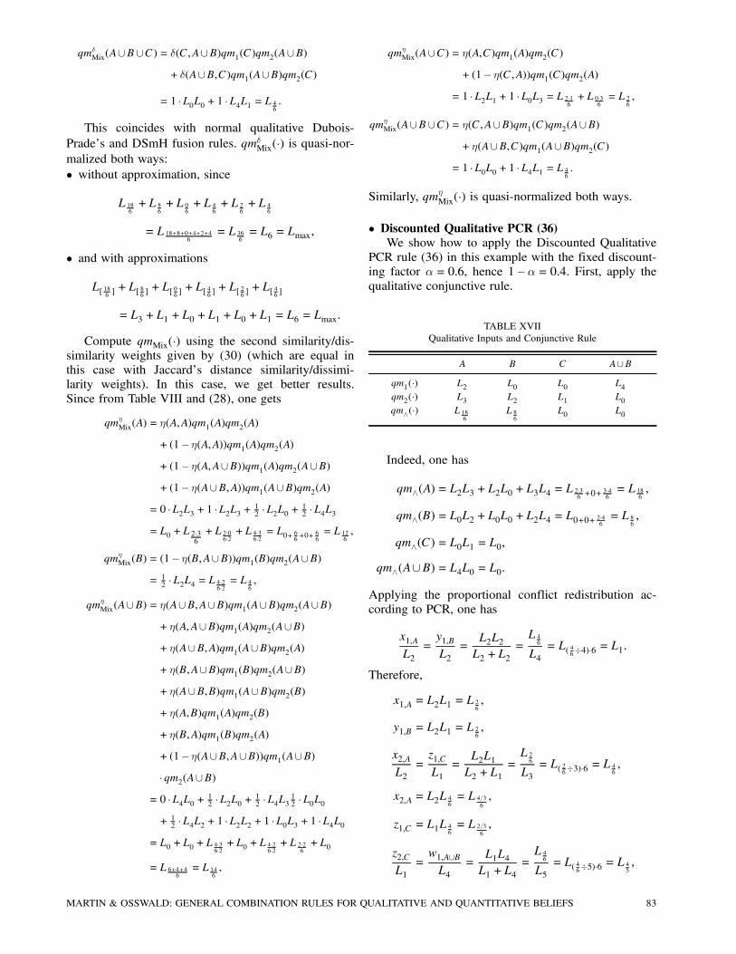
Now let’s apply the qualitative versions of Mixed,Discounted, and Mixed Discounted Quantitative Fusionrules (28), (36) and (44) respectively.

² Qualitative Mixed Dubois-Prade’s ruleFrom (28) and Table VI, one gets:

qm±Mix(A) = ±(A,A)qm1(A)qm2(A)

+ (1¡ ±(A,A))qm1(A)qm2(A)+ (1¡ ±(A,A[B))qm1(A)qm2(A[B)+ (1¡ ±(A[B,A))qm1(A[B)qm2(A)

= 0 ¢L2L3 +1 ¢L2L3 +1 ¢L2L0 +1 ¢L4L3= L0 +L 2¢3

6+L 2¢0

6+L 4¢3

6= L 6

6+L 12

6= L 18

6:

Similarly, qm±Mix(B) = L 86and

qm±Mix(C) = ±(C,C)qm1(C)qm2(C)

+ (1¡ ±(C,C))qm1(C)qm2(C)

= 0 ¢L0L1 +1 ¢L0L1 = L0,

qm±Mix(A[B) = ±(A[B,A[B)qm1(A[B)qm2(A[B)+ ±(A,A[B)qm1(A)qm2(A[B)+ ±(A[B,A)qm1(A[B)qm2(A)+ ±(B,A[B)qm1(B)qm2(A[B)+ ±(A[B,B)qm1(A[B)qm2(B)+ ±(A,B)qm1(A)qm2(B)

+ ±(B,A)qm1(B)qm2(A)

+ (1¡ ±(A[B,A[B))qm1(A[B)qm2(A[B)

= L0 +L0 +L0 +L0 +L0 +1 ¢L2L2 +1 ¢L0L3= L 2¢2

6+L 0¢3

6= L 4

6:

Note: The first five terms of previous sum take value L0since ±1(¢, ¢) = 0 for each of them. Then

qm±Mix(A[C) = ±(A,C)qm1(A)qm2(C)+ (1¡ ±(C,A))qm1(C)qm2(A)

= 1 ¢L2L1 +1 ¢L0L3 = L 2¢16+L 0¢3

6= L 2

6,


qm±Mix(A[B [C) = ±(C,A[B)qm1(C)qm2(A[B)+ ±(A[B,C)qm1(A[B)qm2(C)

= 1 ¢L0L0 +1 ¢L4L1 = L 46:

This coincides with normal qualitative Dubois-Prade’s and DSmH fusion rules. qm±Mix(¢) is quasi-nor-malized both ways:² without approximation, since

L 186+L 8

6+L 0

6+L 4

6+L 2

6+L 4

6

= L 18+8+0+4+2+46

= L 366= L6 = Lmax,

² and with approximations

L[ 186 ]+L[ 86 ] +L[ 06 ] +L[ 46 ] +L[ 26 ] +L[ 46 ]

= L3 +L1 +L0 +L1 +L0 +L1 = L6 = Lmax:

Compute qmMix(¢) using the second similarity/dis-similarity weights given by (30) (which are equal inthis case with Jaccard’s distance similarity/dissimi-larity weights). In this case, we get better results.Since from Table VIII and (28), one gets

qm´Mix(A) = ´(A,A)qm1(A)qm2(A)

+ (1¡ ´(A,A))qm1(A)qm2(A)+ (1¡ ´(A,A[B))qm1(A)qm2(A[B)+ (1¡ ´(A[B,A))qm1(A[B)qm2(A)

= 0 ¢L2L3 +1 ¢L2L3 + 12 ¢L2L0 + 1

2 ¢L4L3= L0 +L 2¢3

6+L 2¢0

6¢2+L 4¢3

6¢2= L0+ 6

6 +0+66= L 12

6,

qm´Mix(B) = (1¡ ´(B,A[B))qm1(B)qm2(A[B)= 1

2 ¢L2L4 = L 4¢26¢2= L 4

6,

qm´Mix(A[B) = ´(A[B,A[B)qm1(A[B)qm2(A[B)+ ´(A,A[B)qm1(A)qm2(A[B)+ ´(A[B,A)qm1(A[B)qm2(A)+ ´(B,A[B)qm1(B)qm2(A[B)+ ´(A[B,B)qm1(A[B)qm2(B)+ ´(A,B)qm1(A)qm2(B)

+ ´(B,A)qm1(B)qm2(A)

+ (1¡ ´(A[B,A[B))qm1(A[B)¢ qm2(A[B)

= 0 ¢L4L0 + 12 ¢L2L0 + 1

2 ¢L4L3 12 ¢L0L0+ 1

2 ¢L4L2 + 1 ¢L2L2 +1 ¢L0L3 +1 ¢L4L0= L0 +L0 +L 4¢3

6¢2+L0 +L 4¢2

6¢2+L 2¢2

6+L0

= L 6+4+46= L 14

6,

qm´Mix(A[C) = ´(A,C)qm1(A)qm2(C)+ (1¡ ´(C,A))qm1(C)qm2(A)

= 1 ¢L2L1 +1 ¢L0L3 = L 2¢16+L 0¢3

6= L 2

6,

qm´Mix(A[B [C) = ´(C,A[B)qm1(C)qm2(A[B)+ ´(A[B,C)qm1(A[B)qm2(C)

= 1 ¢L0L0 +1 ¢L4L1 = L 46:

Similarly, qm´Mix(¢) is quasi-normalized both ways.

² Discounted Qualitative PCR (36)We show how to apply the Discounted Qualitative

PCR rule (36) in this example with the fixed discount-ing factor ®= 0:6, hence 1¡®= 0:4. First, apply thequalitative conjunctive rule.

TABLE XVIIQualitative Inputs and Conjunctive Rule

A B C A[Bqm1(¢) L2 L0 L0 L4qm2(¢) L3 L2 L1 L0qm^(¢) L 18

6L 86

L0 L0

Indeed, one has

qm^(A) = L2L3 +L2L0 +L3L4 = L 2¢36 +0+

3¢46= L 18

6,

qm^(B) = L0L2 +L0L0 +L2L4 = L0+0+ 2¢46= L 8

6,

qm^(C) = L0L1 = L0,

qm^(A[B) = L4L0 = L0:

Applying the proportional conflict redistribution ac-cording to PCR, one has

x1,AL2

=y1,BL2

=L2L2L2 +L2

=L 46

L4= L( 46¥4)¢6 = L1:

Therefore,

x1,A = L2L1 = L 26,

y1,B = L2L1 = L 26,

x2,AL2

=z1,CL1

=L2L1L2 +L1

=L 26

L3= L( 26¥3)¢6 = L 4

6,

x2,A = L2L 46= L 4=3

6,

z1,C = L1L 46= L 2=3

6,

z2,CL1

=w1,A[BL4

=L1L4L1 +L4

=L 46

L5= L( 46¥5)¢6 = L 4

5,


and

z2,C = L1L 45= L 1¢4=5

6= L 0:8

6,

w1,A[B = L4L 45= L 4¢4=5

6= L 3:2

6:

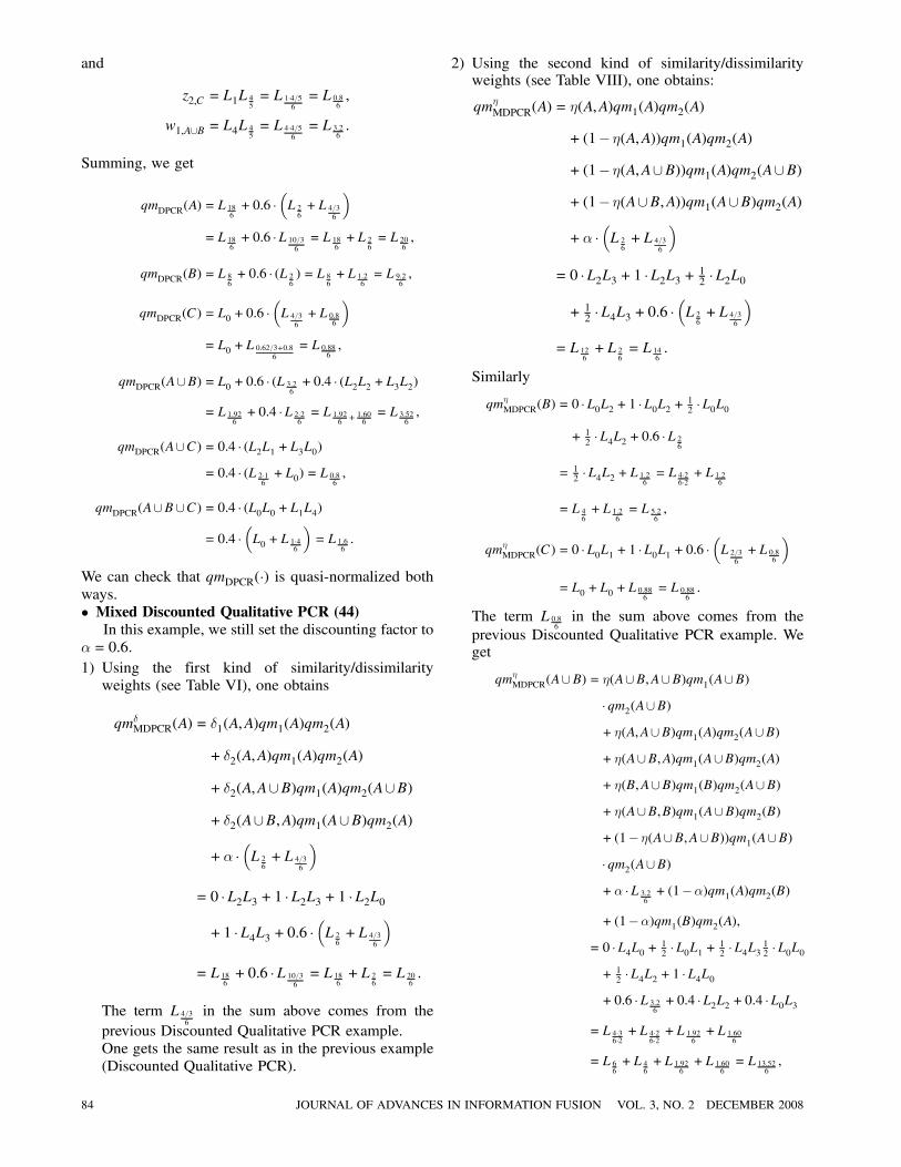
Summing, we get

qmDPCR(A) = L 186+ 0:6 ¢

³L 26+L 4=3

6

´= L 18

6+ 0:6 ¢L 10=3

6= L 18

6+L 2

6= L 20

6,

qmDPCR(B) = L 86+ 0:6 ¢ (L 2

6) = L 8

6+L 1:2

6= L 9:2

6,

qmDPCR(C) = L0 +0:6 ¢³L 4=3

6+L 0:8

6

´= L0 +L 0:62=3+0:8

6= L 0:88

6,

qmDPCR(A[B) = L0 +0:6 ¢ (L 3:26+ 0:4 ¢ (L2L2 +L3L2)

= L 1:926+ 0:4 ¢L 2¢2

6= L 1:92

6 + 1:606= L 3:52

6,

qmDPCR(A[C) = 0:4 ¢ (L2L1 +L3L0)= 0:4 ¢ (L 2¢1

6+L0) = L 0:8

6,

qmDPCR(A[B [C) = 0:4 ¢ (L0L0 +L1L4)

= 0:4 ¢³L0 +L 1¢4

6

´= L 1:6

6:

We can check that qmDPCR(¢) is quasi-normalized bothways.² Mixed Discounted Qualitative PCR (44)In this example, we still set the discounting factor to

®= 0:6.1) Using the first kind of similarity/dissimilarityweights (see Table VI), one obtains

qm±MDPCR(A) = ±1(A,A)qm1(A)qm2(A)

+ ±2(A,A)qm1(A)qm2(A)

+ ±2(A,A[B)qm1(A)qm2(A[B)

+ ±2(A[B,A)qm1(A[B)qm2(A)

+® ¢³L 26+L 4=3

6

´= 0 ¢L2L3 +1 ¢L2L3 +1 ¢L2L0+1 ¢L4L3 +0:6 ¢

³L 26+L 4=3

6

´= L 18

6+ 0:6 ¢L 10=3

6= L 18

6+L 2

6= L 20

6:

The term L 4=36in the sum above comes from the

previous Discounted Qualitative PCR example.One gets the same result as in the previous example(Discounted Qualitative PCR).

2) Using the second kind of similarity/dissimilarityweights (see Table VIII), one obtains:

qm´MDPCR(A) = ´(A,A)qm1(A)qm2(A)

+ (1¡ ´(A,A))qm1(A)qm2(A)+ (1¡ ´(A,A[B))qm1(A)qm2(A[B)+ (1¡ ´(A[B,A))qm1(A[B)qm2(A)

+® ¢³L 26+L 4=3

6

´= 0 ¢L2L3 +1 ¢L2L3 + 1

2 ¢L2L0

+ 12 ¢L4L3 +0:6 ¢

³L 26+L 4=3

6

´= L 12

6+L 2

6= L 14

6:

Similarly

qm´MDPCR(B) = 0 ¢L0L2 +1 ¢L0L2 + 12 ¢L0L0

+ 12 ¢L4L2 +0:6 ¢L 2

6

= 12 ¢L4L2 +L 1:2

6= L 4¢2

6¢2+L 1:2

6

= L 46+L 1:2

6= L 5:2

6,

qm´MDPCR(C) = 0 ¢L0L1 +1 ¢L0L1 +0:6 ¢³L 2=3

6+L 0:8

6

´= L0 +L0 +L 0:88

6= L 0:88

6:

The term L 0:86in the sum above comes from the

previous Discounted Qualitative PCR example. Weget

qm´MDPCR(A[B) = ´(A[B,A[B)qm1(A[B)¢ qm2(A[B)+ ´(A,A[B)qm1(A)qm2(A[B)+ ´(A[B,A)qm1(A[B)qm2(A)+ ´(B,A[B)qm1(B)qm2(A[B)+ ´(A[B,B)qm1(A[B)qm2(B)+ (1¡ ´(A[B,A[B))qm1(A[B)¢ qm2(A[B)+® ¢L 3:2

6+ (1¡®)qm1(A)qm2(B)

+ (1¡®)qm1(B)qm2(A),= 0 ¢L4L0 + 1

2 ¢L0L1 + 12 ¢L4L3 12 ¢L0L0

+ 12 ¢L4L2 +1 ¢L4L0

+0:6 ¢L 3:26+ 0:4 ¢L2L2 +0:4 ¢L0L3

= L 4¢36¢2+L 4¢2

6¢2+L 1:92

6+L 1:60

6

= L 66+L 4

6+L 1:92

6+L 1:60

6= L 13:52

6,


qm´MDPCR(A[C) = (1¡®)qm1(A)qm2(C)+ (1¡®)qm1(C)qm2(A)

= 0:4 ¢L2L1 +0:4 ¢L3L0 = L 0:86,

qm´MDPCR(A[B [C) = (1¡®)qm1(C)qm2(A[B)+ (1¡®)qm1(A[B)qm2(C)

= 0:4 ¢L0L0 +0:4 ¢L4L1 = L 1:66:

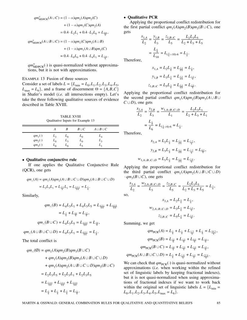
qm´MDPCR(¢) is quasi-normalized without approxima-tions, but it is not with approximations.

EXAMPLE 13 Fusion of three sourcesConsider a set of labels L= fLmin = L0,L1,L2,L3,L4,L5,Lmax = L6g, and a frame of discernment £ = fA,B,Cgin Shafer’s model (i.e. all intersections empty). Let’stake the three following qualitative sources of evidencedescribed in Table XVIII.

TABLE XVIIIQualitative Inputs for Example 13

A B B [C A[B [Cqm1(¢) L2 L0 L0 L4qm2(¢) L0 L3 L0 L3qm3(¢) L0 L0 L5 L1

² Qualitative conjunctive ruleIf one applies the Qualitative Conjunctive Rule

(QCR), one gets

qm^(A) = qm1(A)qm2(A[B [C [D)qm3(A[B [C [D)= L2L3L1 = L 2¢3

6L1 = L 2¢3¢1

6¢6= L 1

6:

Similarly,

qm^(B) = L4L3L1 +L4L3L5 = L 4¢3¢16¢6+L 4¢3¢5

6¢6

= L 26+L 10

6= L 12

6,

qm^(B [C) = L4L3L5 = L 4¢3¢56¢6= L 10

6,

qm^(A[B [C [D) = L4L3L1 = L 4¢3¢16¢6= L 2

6:

The total conflict is

qm^(Ø) = qm1(A)qm2(B)qm3(B [C)+ qm1(A)qm2(B)qm3(A[B [C [D)+ qm1(A)qm2(A[B [C [D)qm3(B [C)

= L2L3L5 +L2L3L1 +L2L3L5

= L 2¢3¢56¢6+L 2¢3¢1

6¢6+L 2¢3¢5

6¢6

= L 56+L 1

6+L 5

6= L 11

6:

² Qualitative PCRApplying the proportional conflict redistribution for

the first partial conflict qm1(A)qm2(B)qm3(B [C), onegets

x1,AL2

=y1,BL3

=z1,B[CL5

=L2L3L5

L2 +L3 +L5

=L 56

L10= L( 56¥10)¢6 = L 3

6:

Therefore,

x1,A = L2L 36= L 2¢3

6¢6= L 1

6,

y1,B = L3L 36= L 3¢3

6¢6= L 1:5

6,

z1,B[C = L5L 36= L 5¢3

6¢6= L 2:5

6:

Applying the proportional conflict redistribution forthe second partial conflict qm1(A)qm2(B)qm3(A[B[C [D), one gets

x2,AL2

=y2,BL3

=w1,A[B[C[D

L1=

L2L3L1L2 +L3 +L1

=L 16

L6= L( 16¥6)¢6 = L 1

6:

Therefore,

x2,A = L2L 16= L 2¢1

6¢6= L 1=3

6,

y2,B = L3L 16= L 3¢1

6¢6= L 1=2

6= L 0:5

6,

w1,A[B[C[D = L1L 16= L 1¢1

6¢6= L 1=6

6:

Applying the proportional conflict redistribution forthe third partial conflict qm1(A)qm2(A[B [C [D)¢ qm3(B [C), one getsx3,AL2

=w2,A[B[C[D

L3=z2,B[CL5

=L2L3L5

L2 +L3 +L5= L 3

6,

so,x3,A = L2L 3

6= L 1

6,

w2,A[B[C[D = L3L 36= L 1:5

6,

z2,B[C = L5L 36= L 2:5

6:

Summing, we get

qmPCR(A) = L 16+L 1

6+L 1=3

6+L 1

6= L 10=3

6,

qmPCR(B) = L 126+L 1:5

6+L 0:5

6= L 14

6,

qmPCR(B [C) = L 106+L 2:5

6+L 2:5

6= L 15

6,

qmPCR(A[B [C [D) = L 26+L 1=6

6+L 1:5

6= L 22=6

6:

We can check that qmPCR(¢) is quasi-normalized withoutapproximations (i.e. when working within the refinedset of linguistic labels by keeping fractional indexes),but it is not quasi-normalized when using approxima-tions of fractional indexes if we want to work backwithin the original set of linguistic labels L= fLmin =L0,L1,L2,L3,L4,L5,Lmax = L6g.


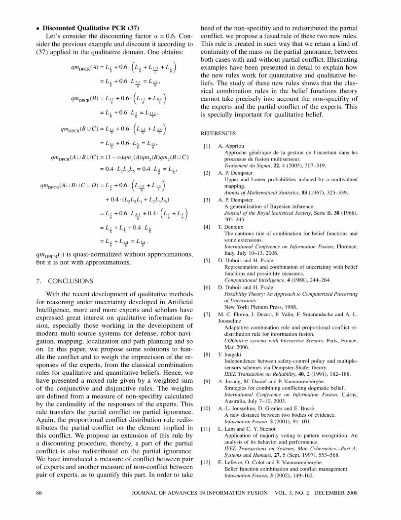
² Discounted Qualitative PCR (37)Let’s consider the discounting factor ®= 0:6. Con-

sider the previous example and discount it according to(37) applied in the qualitative domain. One obtains:

qmDPCR(A) = L 16+ 0:6 ¢

³L 16+L 1=3

6+L 1

6

´= L 1

6+ 0:6 ¢L 7=3

6= L 2:4

6,

qmDPCR(B) = L 126+ 0:6 ¢

³L 1:5

6+L 0:5

6

´= L 1

6+ 0:6 ¢L 2

6= L 13:2

6,

qmDPCR(B [C) = L 106+ 0:6 ¢

³L 2:5

6+L 2:5

6

´= L 10

6+ 0:6 ¢L 5

6= L 13

6,

qmDPCR(A[B [C) = (1¡®)qm1(A)qm2(B)qm2(B [C)= 0:4 ¢L2L3L5 = 0:4 ¢L 5

6= L 2

6,

qmDPCR(A[B [C [D) = L 26+ 0:6 ¢

³L 1=6

6+L 1:5

6

´+0:4 ¢ (L2L3L1 +L2L3L5)

= L 26+ 0:6 ¢L 5=3

6+ 0:4 ¢

³L 16+L 5

6

´= L 2

6+L 1

6+ 0:4 ¢L 6

6

= L 36+L 2:4

6= L 5:4

6:

qmDPCR(¢) is quasi-normalized without approximations,but it is not with approximations.

7. CONCLUSIONS

With the recent development of qualitative methodsfor reasoning under uncertainty developed in ArtificialIntelligence, more and more experts and scholars haveexpressed great interest on qualitative information fu-sion, especially those working in the development ofmodern multi-source systems for defense, robot navi-gation, mapping, localization and path planning and soon. In this paper, we propose some solutions to han-dle the conflict and to weigh the imprecision of the re-sponses of the experts, from the classical combinationrules for qualitative and quantitative beliefs. Hence, wehave presented a mixed rule given by a weighted sumof the conjunctive and disjunctive rules. The weightsare defined from a measure of non-specifity calculatedby the cardinality of the responses of the experts. Thisrule transfers the partial conflict on partial ignorance.Again, the proportional conflict distribution rule redis-tributes the partial conflict on the element implied inthis conflict. We propose an extension of this rule bya discounting procedure, thereby, a part of the partialconflict is also redistributed on the partial ignorance.We have introduced a measure of conflict between pairof experts and another measure of non-conflict betweenpair of experts, as to quantify this part. In order to take

heed of the non-specifity and to redistributed the partialconflict, we propose a fused rule of these two new rules.This rule is created in such way that we retain a kind ofcontinuity of the mass on the partial ignorance, betweenboth cases with and without partial conflict. Illustratingexamples have been presented in detail to explain howthe new rules work for quantitative and qualitative be-liefs. The study of these new rules shows that the clas-sical combination rules in the belief functions theorycannot take precisely into account the non-specifity ofthe experts and the partial conflict of the experts. Thisis specially important for qualitative belief.

REFERENCES

[1] A. AppriouApproche generique de la gestion de l’incertain dans lesprocessus de fusion multisenseur.Traitement du Signal, 22, 4 (2005), 307—319.

[2] A. P. DempsterUpper and Lower probabilities induced by a multivaluedmapping.Annals of Mathematical Statistics, 83 (1967), 325—339.

[3] A. P. DempsterA generalization of Bayesian inference.Journal of the Royal Statistical Society, Serie B, 30 (1968),205—245.

[4] T. DenœuxThe cautious rule of combination for belief functions andsome extensions.International Conference on Information Fusion, Florence,Italy, July 10—13, 2006.

[5] D. Dubois and H. PradeRepresentation and combination of uncertainty with belieffunctions and possibility measures.Computational Intelligence, 4 (1988), 244—264.

[6] D. Dubois and H. PradePossibility Theory: An Approach to Computerized Processingof Uncertainty.New York: Plenum Press, 1988.

[7] M. C. Florea, J. Dezert, P. Valin, F. Smarandache and A. L.JousselmeAdaptative combination rule and proportional conflict re-distribution rule for information fusion.COGnitive systems with Interactive Sensors, Paris, France,Mar. 2006.

[8] T. InagakiIndependence between safety-control policy and multiple-sensors schemes via Dempster-Shafer theory.IEEE Transaction on Reliability, 40, 2 (1991), 182—188.

[9] A. Josang, M. Daniel and P. VannoorenbergheStrategies for combining conflicting dogmatic belief.International Conference on Information Fusion, Cairns,Australia, July 7—10, 2003.

[10] A.-L. Jousselme, D. Grenier and E. BosseA new distance between two bodies of evidence.Information Fusion, 2 (2001), 91—101.

[11] L. Lam and C. Y. SuenotApplication of majority voting to pattern recognition: Ananalysis of its behavior and performance.IEEE Transactions on Systems, Man Cybernetics–Part A:Systems and Humans, 27, 5 (Sept. 1997), 553—568.

[12] E. Lefevre, O. Colot and P. VannoorenbergheBelief function combination and conflict management.Information Fusion, 3 (2002), 149—162.


[13] X. Li, X. Huang, J. Dezert and F. SmarandacheEnrichment of qualitative belief for reasoning under uncer-tainty.International Conference on Information Fusion, QuebecCity, Canada, July 9—12, 2007.

[14] A. Martin and C. OsswaldA new generalization of the proportional conflict redistri-bution rule stable in terms of decision.Applications and Advances of DSmT for Information Fusion,Book 2, American Research Press, Rehoboth, F. Smaran-dache and J. Dezert (Eds.), 2006, 69—88.

[15] A. Martin and C. OsswaldToward a combination rule to deal with partial conflict andspecificity in belief functions theory.International Conference on Information Fusion, Quebec,Canada, July 9—12, 2007.

[16] C. Osswald and A. MartinUnderstanding the large family of Dempster-Shafer the-ory’s fusion operators–a decision-based measure.International Conference on Information Fusion, Florence,Italy, July 10—13, 2006.

[17] G. ShaferA Mathematical Theory of Evidence.Princeton University Press, 1976.

[18] F. Smarandache and J. Dezert (Eds.)Applications and Advances of DSmT for Information Fusion(Collected works).American Research Press, Rehoboth, 2004. http://www.gallup.unm.edu/»smarandache/DSmT-book1.pdf.

[19] F. Smarandache and J. Dezert (Eds.)Applications and Advances of DSmT for Information Fusion(Collected works, vol. 2.)American Research Press, Rehoboth, 2006. http://www.gallup.unm.edu/»smarandache/DSmT-book2.pdf.

[20] F. Smarandache and J. Dezert (Eds.)Applications and Advantages of DSmT for Information Fu-sion (Collected works, vol. 3).American Research Press, Rehoboth, 2009, http://www.gallup.unm.edu/»smarandache/DSmT-book3.pdf.

[21] F. Smarandache and J. DezertInformation fusion based on new proportional conflict re-distribution rules.International Conference on Information Fusion, Philadel-phia, PA, July 25—29, 2005.

[22] F. Smarandache and J. DezertProportional conflict redistribution rules for informationfusion.Applications and Advances of DSmT for Information Fusion,Book 2, American Research Press, Rehoboth, F. Smaran-dache and J. Dezert (Eds.), 2006, 3—68.

[23] F. SmarandacheAn in-depth look at quantitative information fusion rules.In Applications and Advances of DSmT for InformationFusion, Book 2, American Research Press, Rehoboth, F.Smarandache and J. Dezert (Eds.), 2006, 205—235 (origi-nally presented at NASA Langley Research Center, Hamp-ton, VA, on Nov. 5, 2005).

[24] F. Smarandache and J. DezertQualitative belief conditioning rules (QBCR).International Conference on Information Fusion, QuebecCity, Canada, July 9—12, 2007.

[25] Ph. SmetsConstructing the pignistic probability function in a contextof uncertainty.Uncertainty in Artificial Intelligence, 5 (1990), 29—39.

[26] Ph. SmetsThe combination of evidence in the transferable beliefmodel.IEEE Transactions on Pattern Analysis and Machine Intelli-gence, 12, 5 (1990), 447—458.

[27] Ph. SmetsBelief functions: The disjunctive rule of combination andthe generalized Bayesian theorem.International Journal of Approximate Reasoning, 9 (1993),1—35.

[28] Ph. Smets and R. KennesThe transferable belief model.Artificial Intelligent, 66 (1994), 191—234.

[29] Ph. SmetsThe ®-junctions: The commutative and associative non in-teractive combination operators applicable to belief func-tions.Qualitative and Quantitative Practical Reasoning, SpringerVerlag, D. Gabbay and R. Kruse and A. Nonnengart andH. J. Ohlbacg, Berlin, 1997, 131—153.

[30] K. Sentz and S. FersonCombination of Evidence in Dempster-Shafer Theory.SANDIA Tech. Report, SAND2002-0835, Apr. 2002. 96pages.

[31] L. Xu, A. Krzyzak and C. Y. SuenMethods of combining multiple classifiers and their appli-cation to handwriting recognition.IEEE Transactions on Systems, Man Cybernetics, 22, 3 (May1992), 418—435.

[32] R. R. YagerHedging in the combination of evidence.Journal of Information and Optimization Science, 4, 1 (1983),73—81.

[33] R. R. YagerOn the relationships of methods of aggregation of evidencein expert systems.Cybernetics and Systems, 16 (1985), 1—21.

[34] R. R. YagerOn the Dempster-Shafer framework and new combinationrules.Informations Sciences, 41 (1987), 93—137.

[35] L. ZadehFuzzy sets as a basis for a theory of possibility.Fuzzy Sets and Systems, 1, 3 (1978), 3—28.

[36] L. ZadehOn the validity of Dempster’s rule of combination.Memo M 79/24, Univ. of California, Berkeley, 1979.


Arnaud Martin was born in Bastia, France in 1974. He received the Ph.D. degreein signal processing (2001), and the M.S. degree in probability (1998) from theUniversity of Rennes, France.He worked on speech recognition for three years (1998—2001) at France Telecom

R&D, Lannion, France. He worked in the Department of Statistics and Data Mining(STID) of the IUT of Vannes, France, as temporary assistant professor (ATER) fortwo years (2001—2003). In 2003, he joined the Laboratory E3I2: EA3876 at theENSIETA, Brest, France, as a teacher and researcher. Dr. Arnaud Martin teachesmathematics, data fusion, data mining, signal processing, and computer sciences.Today, his research interests are mainly related to the belief functions for patternrecognition of real data and include data fusion, data mining, signal processing,especially for sonar and radar data.

Christophe Osswald was born in Orleans, France, in 1975. He received the Ph.D.degree in mathematics and computer science (2003) from the EHESS–Ecole desHautes Etudes en Sciences Sociales–after three years of research on classification,similarity analysis, and hypergraphs at the Laboratory IASC of the ENST Bretagne.He is an engineer graduated from the Ecole Polytechnique (1997) and the ENSTBretagne (1999), and received the M.S. degree in mathematics and computer scienceapplied to social sciences.He is a teacher and researcher at the ENSIETA in the Laboratory E3I2: EA3876,

Brest, France. His research interests are related to data fusion, mostly through belieffunctions, and also to classification, graphs and hypergraphs theory, algorithmiccomplexity, and decision support.


Jean Dezert was born in l’Hay les Roses, France, on August 25, 1962. He receivedthe electrical engineering degree from the Ecole Française de RadioelectriciteElectronique and Informatique (EFREI), Paris, in 1985, the D.E.A. degree in 1986from the University Paris VII (Jussieu), and his Ph.D. from the University Paris XI,Orsay, in 1990, all in automatic control and signal processing.During 1986—1990 he was with the Systems Department at the French Aerospace

Research Lab (ONERA), Châtillon, France, and did research in multisensor multitar-get tracking (MS-MTT). During 1991—1992, he visited the Department of Electricaland Systems Engineering, University of Connecticut, Storrs, as a European SpaceAgency (ESA) Postdoctoral Research Fellow. During 1992—1993 he was teachingassistant in electrical engineering at the University of Orleans, France. Since 1993,he is a senior research scientist in the Information Modelling and Processing Depart-ment (DTIM) at ONERA. His current research interests include autonomous navi-gation, estimation theory, stochastic systems theory and its applications to MS-MTT,information fusion, plausible reasoning and non-standard Logics. Dr. Jean Dezertis developing since 2001 with Professor Smarandache a new theory of plausibleand paradoxical reasoning for information fusion (DSmT) and has edited two text-books (collected works) devoted to this new emerging research field published byAmerican Research Press, Rehoboth in 2004 and 2006 respectively and a third vol-ume is in preparation (see http://www.gallup.unm.edu/»smarandache/DSmT.htm).He owns one international patent in the autonomous navigation field and has pub-lished several papers tracking and fusion in international conferences and journals.He was member of IEEE and of Eta Kappa Nu, serves as reviewer for differentInternational Journals, taught courses on MS-MTT and Data Fusion at the FrenchENSTA Engineering School, collaborates for the development of the InternationalSociety of Information Fusion (ISIF) since 1998, and has served as Local Arrange-ments Organizer for Fusion 2000 Conference in Paris. He has been involved in theTechnical Program Committees of Fusion 2001—2007 International Conferences.Since 2001, he is a member of the board of the International Society of Informa-tion Fusion (http://www.isif.org) and serves in ISIF executive board. He served asexecutive vicepresident of ISIF in 2004. Dr. Dezert gave several invited seminars,lectures and tutorials on Data Fusion and Tracking during recent past years–thelast recent was given at Fusion 2008 in Cologne, Germany on July 2008.

Florentin Smarandache is a Professor and Chair of Math & Sciences Departmentat the University of New Mexico. He published over 75 books and 150 articlesand notes in mathematics, physics, philosophy, psychology, literature, and rebus. Inmathematics, his research is in number theory, non-Euclidean geometry, syntheticgeometry, algebraic structures, statistics, neutrosophic logic and set (generalizationsof fuzzy logic and set respectively), and neutrosophic probability (generalization ofclassical and imprecise probability). Other contributions are to nuclear and particlephysics, neutrosophy (a generalization of dialectics), law of sensations and stimuli,and especially to information fusion.


Documents

General Combination Rules for Qualitative and Quantitative Beliefs