Embed Size (px)
Citation preview
Gene Maps Linearization using Genomic Rearrangement
Distances
Guillaume Blin, Eric Blais, Danny Hermelin, Pierre Guillon, Mathieu
Blanchette, Nadia El-Mabrouk
To cite this version:
Guillaume Blin, Eric Blais, Danny Hermelin, Pierre Guillon, Mathieu Blanchette, et al.. GeneMaps Linearization using Genomic Rearrangement Distances. Journal of Computational Biol-ogy, Mary Ann Liebert, 2007, 14 (4), pp.394-407. <hal-00619755>
HAL Id: hal-00619755
https://hal-upec-upem.archives-ouvertes.fr/hal-00619755
Submitted on 22 Oct 2011
HAL is a multi-disciplinary open accessarchive for the deposit and dissemination of sci-entific research documents, whether they are pub-lished or not. The documents may come fromteaching and research institutions in France orabroad, or from public or private research centers.
L’archive ouverte pluridisciplinaire HAL, estdestinee au depot et a la diffusion de documentsscientifiques de niveau recherche, publies ou non,emanant des etablissements d’enseignement et derecherche francais ou etrangers, des laboratoirespublics ou prives.
Gene Maps Linearization using Genomic Rearrangement
Distances
Guillaume Blin∗ Eric Blais† Danny Hermelin‡ Pierre Guillon§
Mathieu Blanchette¶ Nadia El-Mabrouk‖
Abstract
A preliminary step to most comparative genomics studies is the annotation of chro-
mosomes as ordered sequences of genes. Different genetic mapping techniques often
give rise to different maps with unequal gene content and sets of unordered neighboring
genes. Only partial orders can thus be obtained from combining such maps. However,
once a total order O is known for a given genome, it can be used as a reference to order
genes of a closely related species characterized by a partial order P . Our goal is to find
a linearization of P that is as close as possible to O, in term of a given genomic dis-
tance. We first prove NP-completeness complexity results considering the breakpoint
and the common interval distances. We then focus on the breakpoint distance and
give a dynamic programming algorithm whose running time is exponential for general
partial orders, but polynomial when the partial order is derived from a bounded num-
ber of genetic maps. A time-efficient greedy heuristic is then given for the general case
∗IGM-LabInfo, UMR CNRS 8049, Universite de Marne-la-Vallee, France. [email protected]†McGill Centre for Bioinformatics, McGill University, H3A 2B4, Canada. [email protected]‡Department of Computer Science, University of Haifa, Mount Carmel, Haifa, Israel. [email protected]§IGM-LabInfo, UMR CNRS 8049, Universite de Marne-la-Vallee, France. [email protected]¶McGill Centre for Bioinformatics, McGill University, H3A 2B4, Canada. [email protected]‖DIRO, Universite de Montreal, H3C 3J7, Canada. [email protected]
1
and is empirically shown to produce solutions within 10% of the optimal solution, on
simulated data. Applications to the analysis of grass genomes are presented.
1 Introduction
Despite the increase in the number of sequencing projects, the choice of candidates for com-
plete genome sequencing is usually limited to a few model organisms and species with major
economical impact. For example, the rice genome is the only crop genome that has been
completely sequenced. Other grasses of major agricultural importance such as maize and
wheat are unlikely to be sequenced in the short term, due to their large size and highly
repetitive composition. In this case, all we have are partial maps produced by recombina-
tion analysis, physical imaging and other mapping techniques that are inevitably missing
some genes (or other markers) and fail to resolve the ordering of some sets of neighboring
genes. Only partial orders can thus be obtained from combining such maps. The question is
then to find an appropriate order for the unresolved sets of genes. This is important not only
for genome annotation, but also for the study of evolutionary relationships between species.
Once total orders have been identified, the classical genome rearrangement approaches can
be used to infer divergence histories in terms of global mutations such as inversions, transpo-
sitions and translocations (Bergeron et al., 2004; Bourque et al., 2005b; El-Mabrouk, 2000;
Hannenhalli and Pevzner, 1999; Pevzner and Tesler, 2003; Tang and Moret, 2003).
In a recent study, Sankoff et. al. generalized the rearrangement by reversal problem to
handle two partial orders (Sankoff et al., 2005; Zheng et al., 2005). The idea was to find two
total orders with the minimal reversal distance. The problem has been conjectured NP-hard,
and a branch-and-bound algorithm has been developed for this purpose. The difficulty of this
2
problem is partly due to the fact that both compared genomes have partially resolved gene
orders. However, once a total order is known for a given genome (for example a completely
sequenced genome), it can be used as a reference to order markers of closely related species.
Given a reference genome characterized by a total order O and a related genome charac-
terized by a partial order P , the goal is to find a permutation consistent with P minimizing
a given genomic distance with respect to O. We consider the breakpoint distance, which is
the simplest measure of gene order conservation usually used as a first attempt to solve any
genome rearrangement problem. Moreover, half the breakpoint distance gives a lower bound
for the inversion distance. We also consider a more general measure of synteny, the common
interval distance, that has been widely studied in the last two years (Blin and Rizzi, 2005;
Figeac and Varre, 2004; Berard et al., 2004; Bourque et al., 2005a; Blin et al., 2006).
After introducing the basic concepts in Section 2, we prove NP-complete results in Sec-
tion 3. Section 4 then presents two exact dynamic programming algorithms for the break-
point distance. The first algorithm applies to arbitrary partial orders. Its running time
is exponential in the number of genes, but when the partial order is the intersection of a
bounded number of genetic maps of bounded width, it runs in polynomial time. The second
is a linear time algorithm that applies only to partial orders derived from a single genetic
map. Section 5 then presents a fast and accurate heuristic for the general case. We finally
report results on simulated data, and applications to grass genetic maps in Section 6.
2 A graph representation of gene maps
Hereafter, we refer to elementary units of a genetic map as genes, although they could in
reality be any kind of markers. Moreover, as the transcriptional orientation of genes is
3
usually missing from genetic maps, we consider unsigned genes.
Formally, a genetic map is represented as an ordered sequence of gene subsets or blocks
B1, B2, . . . , Bq, where for each 1 ≤ i ≤ q, genes belonging to block Bi are incomparable
among themselves, but precede those in blocks Bi+1, . . . , Bq and succeed those in blocks
B1, . . . , Bi−1. For example, in Figure 1.a, {4, 5} is a block, indicating that the order of
genes 4 and 5 is left undecided. Maps M1, . . . ,Mm obtained from various protocols can be
combined to form a more complex partial order P on the union set of the genes of all maps
as follows: a gene a precedes a gene b in P if there exists a map Mi where a precedes b.
However, combining maps can be a problem in itself, due to possible inconsistencies which
would create precedence cycles (e.g. a precedes b in M1 but b precedes a in M2), or the
presence of multiple loci (markers that are assigned to different positions in the same map).
These issues have been considered in previous studies (Yap et al., 2003; Zheng et al., 2005;
Sankoff et al., 2005), and a software is available for combining genetic maps (Jackson et al.,
2005). In this paper, we assume that the partial order P is already known.
A partial order P is represented as a DAG (directed acyclic graph) (VP , EP ), where VP is
the set of vertices (genes) and EP is the edge set representing the available order information
(Figure 1 using data from “IBM2 neighbors 2004” (Polacco and E., 2002), “Paterson 2003”
(Bowers et al., 2003) and “Klein 2004” (Menz et al., 2002)). EP is a minimum set of edges,
in the sense that an edge can not be deduced by transitivity from others.
2.1 Preliminary definitions
Let P be a partial order represented by a DAG (VP , EP ). A vertex a is P -adjacent to a
vertex b (denoted by a <P b) if there is an edge from a to b, and a precedes b (denoted
4
83
4
57 14
15
161721
18
192010 121311
9
1
62 11 12 16 208
1 3
4
57
62
14
15
161721
18
192010 12138 11
9
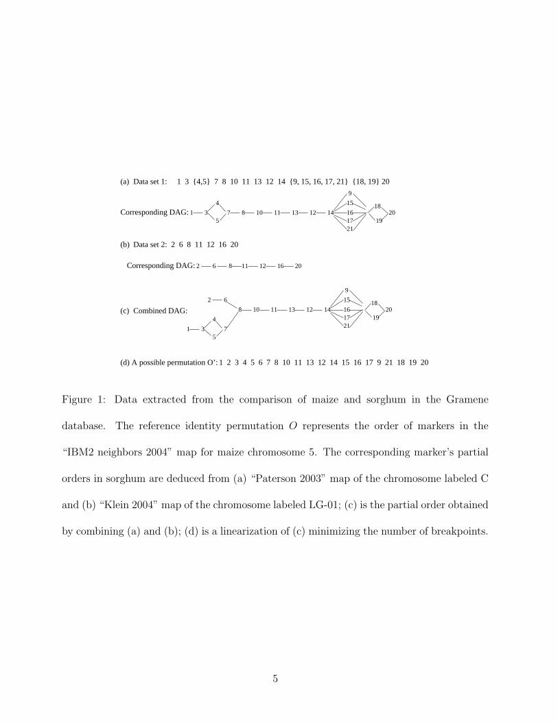
Data set 1: 1 3 {4,5} 7 8 10 11 13 12 14 {9, 15, 16, 17, 21} {18, 19} 20(a)
Data set 2: 2 6 8 11 12 16 20(b)
Combined DAG: (c)
(d) A possible permutation O’: 1 2 3 4 5 6 7 8 10 11 13 12 14 15 16 17 9 21 18 19 20
Corresponding DAG:
Corresponding DAG:
Figure 1: Data extracted from the comparison of maize and sorghum in the Gramene
database. The reference identity permutation O represents the order of markers in the
“IBM2 neighbors 2004” map for maize chromosome 5. The corresponding marker’s partial
orders in sorghum are deduced from (a) “Paterson 2003” map of the chromosome labeled C
and (b) “Klein 2004” map of the chromosome labeled LG-01; (c) is the partial order obtained
by combining (a) and (b); (d) is a linearization of (c) minimizing the number of breakpoints.
5
by a �P b) if there is a directed path from a to b. The vertices a and b are incomparable
(denoted by a ∼P b) if neither a �P b nor b �P a. A total order or permutation is just a
partial order with no incomparable vertices.
A linearization of P is a permutation O′ on the same set of genes, such that a �P b ⇒
a �O′ b. Given a partial order P and a permutation O on the same set of genes, our
goal is to find a linearization O′ of P , as close as possible to O. We consider two distance
measures: the number bkpts(O,O′) of breakpoints of O′ with respect to O, and the number
ICommon(O,O′) of common intervals of O and O′.
Formally, a breakpoint of O′ with respect to O is a pair (a, b) of vertices that are O′-
adjacent but not O-adjacent. For example, the pair (8, 10) is the leftmost breakpoint in the
permutation O′ (Figure 1.(d)) w.r.t the identity.
Let O and O′ be two permutations on the set VP of genes. A subset V of VP is a common
interval of O and O′ if and only if both O and O′ contain a sub-permutation (set of adjacent
genes) whose gene content is exactly V . In other words, the vertices in V are adjacent
in both O and O′, but not necessarily in the same order. For example, in Figure 1.(d),
{10, 11, 13, 12, 14} is a common interval of O and O′. In the following, a common interval
is either represented as a set V of vertices or as an interval [a, b] of O′ where a, b ∈ V , a
precedes and b succeeds all the vertices of V .
2.2 Problems
Formally we define the two following problems:
6
Minimum-Breakpoint Linearization (MBL) problem
Given: A partial order P and a permutation O on the set of genes {1, 2, . . . , n},
Find: A linearization of P into a permutation O′ so that bkpts(O,O′) is minimized.
Maximum-Common Interval Linearization (MCIL) problem
Given: A partial order P and a permutation O on the set of genes {1, 2, . . . , n},
Find: A linearization of P into a permutation O′ so that ICommon(O,O′) is maximized.
One may note that minimizing the number of breakpoints is equivalent to maximizing
the number of O-adjacencies. Moreover, as an adjacency is a common interval of size 2, the
MCIL problem is a generalization of the MBL problem.
W.l.o.g, we assume from now on that O is the identity permutation (1, 2, . . . , n).
Remark 1 (Signed genes and unequal gene content) All hardness results and algo-
rithmic solutions developed in this paper hold for signed genes as well, using the classical
definition of breakpoints: a breakpoint of O′ with respect to O is a pair (a, b) such that
a <O′ b, but neither a ≮O b nor −b ≮O −a. As for common intervals, the same definition
holds in the case of signed permutations. Moreover, from a theoretical point of view, all
algorithmic solutions developed are also applicable to a partial order and a permutation with
unequal gene content. However, as the goal is to find an appropriate order of a genetic map
G using a reference genome H, only common genes of G and H are of interest.
7
3 Hardness results
In this section, we prove that the decision version of both the MBL and the MCIL problems is
NP-complete. The properties of partial orders linearization that are presented in this section
and that are required to prove the hardness result are also useful in the understanding of
the two exact dynamic programming algorithms presented in the next section.
We propose a reduction from the NP-complete problem Maximum Independent Set
(Garey and Johnson, 1979): given a graph G = (V,E) and an integer k, can one find an
independent set of vertices of G – i.e. a set V ′ ⊆ V such that no two vertices of V ′ are
connected by an edge in E – of cardinality greater than or equal to k ?
We initially note that the MBL and the MCIL problems are in NP since given a permu-
tation O and a linearization O′ of P , one can compute the number of breakpoints in linear
time and the number of common intervals in quadratic time.
For convenience, we define a reduction from a slightly different set of instances for the
Maximum Independent Set problem: connected graphs. This can be done w.l.o.g.
since the problem is still NP-complete in that case. Let G = (V,E) be a connected
graph of n vertices. We define the permutation O and the partial order P as follows.
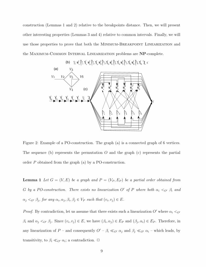
The permutation O is defined as a string O = δ α1 β1 γ1 α2 β2 γ2 . . . αn βn γn χ ε,
and the partial order P as a DAG P = (VP , EP ) with VP = {δ, α1, α2, . . . , αn, β1, β2, . . .,
βn, γ1, γ2, . . . , γn, χ, ε} and EP = {(γ1, δ), (δ, χ)} ∪ {(γi+1, γi)|1 ≤ i < n} ∪ {(χ, αi), (χ, βi)|
1 ≤ i ≤ n}∪{(βi, αj), (βj, αi)|∀(vi, vj) ∈ E}∪{(αi, ε), (βi, ε)|1 ≤ i ≤ n}. In the following, we
will refer to any such construction as a PO-construction. An illustration of a PO-construction
of a graph G with 6 vertices is illustrated in Figure 2.
First, let us present some interesting properties of any instance (O,P ) obtained by a PO-
8
construction (Lemmas 1 and 2) relative to the breakpoints distance. Then, we will present
other interesting properties (Lemmas 3 and 4) relative to common intervals. Finally, we will
use those properties to prove that both the Minimum-Breakpoint Linearization and
the Maximum-Common Interval Linearization problems are NP-complete.
Figure 2: Example of a PO-construction. The graph (a) is a connected graph of 6 vertices.
The sequence (b) represents the permutation O and the graph (c) represents the partial
order P obtained from the graph (a) by a PO-construction.
Lemma 1 Let G = (V,E) be a graph and P = (VP , EP ) be a partial order obtained from
G by a PO-construction. There exists no linearization O′ of P where both αi <O′ βi and
αj <O′ βj, for any αi, αj, βi, βj ∈ VP such that (vi, vj) ∈ E.
Proof. By contradiction, let us assume that there exists such a linearization O ′ where αi <O′
βi and αj <O′ βj. Since (vi, vj) ∈ E, we have (βi, αj) ∈ EP and (βj, αi) ∈ EP . Therefore, in
any linearization of P – and consequently O′ – βi �O′ αj and βj �O′ αi – which leads, by
transitivity, to βi �O′ αi; a contradiction. 2
9
Lemma 2 Let G = (V,E) be a graph of n vertices, O and P = (VP , EP ) be respectively a
permutation and a partial order obtained from G by a PO-construction. Given any lineariza-
tion O′ of P , bkpts(O,O′) = (3n + 2) − k where k is the number of pairs (αi, βi) such that
αi <O′ βi.
Proof. By construction, in O, (i) δ <O α1 <O β1 <O γ1, (ii) ∀1 < i ≤ n, γi−1 <O αi <O
βi <O γi and (iii) γn <O χ <O ε. In any linearization O′ of P , (i) γ1 <O′ δ, (ii) ∀1 < i ≤ n,
γi <O′ γi−1, (iii) δ <O′ χ and (iv) either αj <O′ ε or βj <O′ ε for a given 1 ≤ j ≤ n.
Therefore, in any linearization O′ of P , the only adjacencies that can be preserved are the
ones of the form αi <O βi for some 1 ≤ i ≤ n. Let k be the number of pairs (αi, βi) such that
αi <O′ βi. If k = 0 then no adjacencies at all are preserved, therefore bkpts(O,O′) = (3n+2).
Consequently, if k > 0 then bkpts(O,O′) = (3n + 2) − k. 2
Lemmas 1 and 2 will be used afterwords in the proof of the NP-completeness of the
MBL-problem. We now state some properties relative to the types and maximum numbers
of common intervals between the permutation and any linearization of the partial order
obtained by a PO-construction.
Lemma 3 Let G = (V,E) be a graph of n vertices, O and P = (VP , EP ) be respectively
a permutation and a partial order obtained from G by a PO-construction. Given any lin-
earization O′ of P , any non-trivial common interval between O and O′ is one of the following:
{[δ, χ], [δ, ε], [αi, βi]}, where 1 ≤ i ≤ n .
Proof. Let us first characterize any common interval of size greater or equal to 3. By
construction, considering O as the reference, any interval of that size is of one of the following
forms: (i) {αj, βj, γj}, (ii) {βi, γi, αi+1}, (iii) {γi, αi+1, βi+1}, (iv) {γn, χ, ε}, (v) {δ, α1, β1}
10
for 1 ≤ j ≤ n and 1 ≤ i < n.
Since, by construction, in any linearization O′ of P γi �O′ δ <O′ χ �O′ {αi, βi} for
1 ≤ i ≤ n, any common interval containing an α and a γ has to contain also χ and δ.
Therefore, there is no common interval of type (i), (ii) or (iii); the smallest common interval
including simultaneously an α and a γ is indeed [δ, χ].
By construction, in any linearization O′ of P , γn �O′ δ <O′ χ. Thus, any common
interval of type (iv) has to contain also δ. Therefore, there is no common interval of type
(iv); the smallest common interval including simultaneously γn, ε and χ is indeed [δ, ε].
Finally, in any linearization O′ of P , δ <O′ χ �O′ {αi, βi} for any 1 ≤ i ≤ n. Therefore,
any common interval of type (v) has to contain also χ. Therefore, there is no common
interval of type (v); the smallest common interval including simultaneously δ and an α or a
β is indeed [δ, χ].
We just proved that any common interval of size greater or equal than 3 is either [δ, χ]
or [δ, ε]. Let us now characterize the common intervals of size 2. By construction any of
these intervals is of one of the following forms: (i) {δ, α1}, (ii) {αi, βi}, (iii) {βi, γi}, (iv)
{γj, αj+1}, (v) {γn, χ}, (vi) {χ, ε} for 1 ≤ i ≤ n and 1 ≤ j < n.
By construction, in any linearization O′ of P , γi �O′ δ <O′ χ �O′ {αi, βi} for any
1 ≤ i ≤ n. Therefore, any common interval of type (i), (iii), (iv) or (v) has to contain also
χ and δ. Therefore, there is no common interval of those types. Finally, in any linearization
O′ of P , χ �O′ {αi, βi} �O′ ε. Whereas in O, βn <O′ γn <O′ χ <O′ ε. Therefore, any
common interval of type (vi) has to contain also δ and γn.
We have thus proved that given any linearization O′ of P , any common interval of size
at least two between O and O′ is one of the following: {[δ, χ], [δ, ε], [αi, βi]} where 1 ≤ i ≤ n.
11
2
Lemma 4 Let G = (V,E) be a graph of n vertices, O and P = (VP , EP ) be respectively a
permutation and a partial order obtained from G by a PO-construction. Given any lineariza-
tion O′ of P , ICommon(O,O′) = k + 3n + 5 where k is the number of pairs (αi, βi) such
that αi <O′ βi or βi <O′ αi.
Proof. Let (vi, vj) ∈ E. By construction, in P we have βj <P αi and βi <P αj. Let O′ be a
linearization of P s.t. αi <O′ βi. In O′, [αi, βi] is thus a common interval between O and O′.
We will prove that [αj, βj] cannot be a common interval between O and O′.
Indeed, there are three cases: αj <O′ βj, βj <O′ αj or none of those two. By Lemma 1,
the first case is not possible. Therefore, consider first that βj <O′ αj. Then, in O′ we have
βj �O′ αi <O′ βi �O′ αj. Consequently, [αj, βj] cannot be a common interval. Similarly,
consider that in O′, βi <O′ αi. In O′, [αi, βi] is a common interval between O and O′. If
αj <O′ βj, in O′ we have βi �O′ αj <O′ βj �O′ αi; [αi, βi] is not a common interval anymore,
a contradiction. If βj <O′ αj then by construction we have βj �O′ βi <O′ αi �O′ αj. In both
cases, [αj, βj] cannot be a common interval. Therefore, by Lemma 3, in any linearization of
P , there are k + 2 + 3(n + 1) common intervals where k is the number of pairs (αi, βi) such
that αi <O′ βi or βi <O′ αi.
2
We now turn to the proof of the following theorems.
Theorem 1 A connected graph G = (V,E) admits an independent set of vertices V ′ ⊆ V of
cardinality greater than or equal to k if and only if there exists a linearization O ′ of P such
that bkpts(O,O′) ≤ (3n + 2) − k, where O and P result from a PO-construction of G.
12
Proof. (⇒) Let V ′ ⊆ V such that |V ′| ≥ k and V ′ is an independent set. Let O′ be a
linearization of P defined by O′ = P1 δ χ P2 P3 P4 ε where:
• P1 is the linearization of the subset of vertices V ′1 = {γi|1 ≤ i ≤ n} such that ∀1 < i ≤
n, γi <P1γi−1;
• P2 is any linearization of the subset of vertices V ′2 = {βi|vi ∈ V − V ′};
• P3 is any linearization of the subset of vertices V ′3 = {αi, βi|vi ∈ V ′} such that ∀vi ∈ V ′,
αi <P3βi;
• P4 is any linearization of the subset of vertices V ′4 = {αi|vi ∈ V − V ′}.
For example, given the instances illustrated in Figure 2 and an independent set V ′ =
{1, 3, 4}, O′ is defined by:
O′ = γ6 γ5 γ4 γ3 γ2 γ1 δ χ β2 β5 β6 α1 β1 α3 β3 α4 β4 α2 α5 α6 ε.
By Lemma 2, we can affirm that bkpts(O,O′) = (3n + 2) − |V ′|. Since, by hypothesis,
|V ′| ≥ k, we obtain bkpts(O,O′) ≤ (3n + 2) − k.
(⇐) Suppose we have a linearization O′ of P such that bkpts(O,O′) ≤ (3n + 2)− k. Let
V ′ ⊆ V be the set of vertices such that:
∀(αi, βi) such that αi <O′ βi, add vi to V ′
By Lemma 1, we can affirm that V ′ is an independent set. Let us verify that |V ′| ≥ k.
By Lemma 2, bkpts(O,O′) = (3n + 2) − k where k is the number of pairs (αi, βi) such that
αi <O′ βi. Therefore, we obtain |V ′| = k. 2
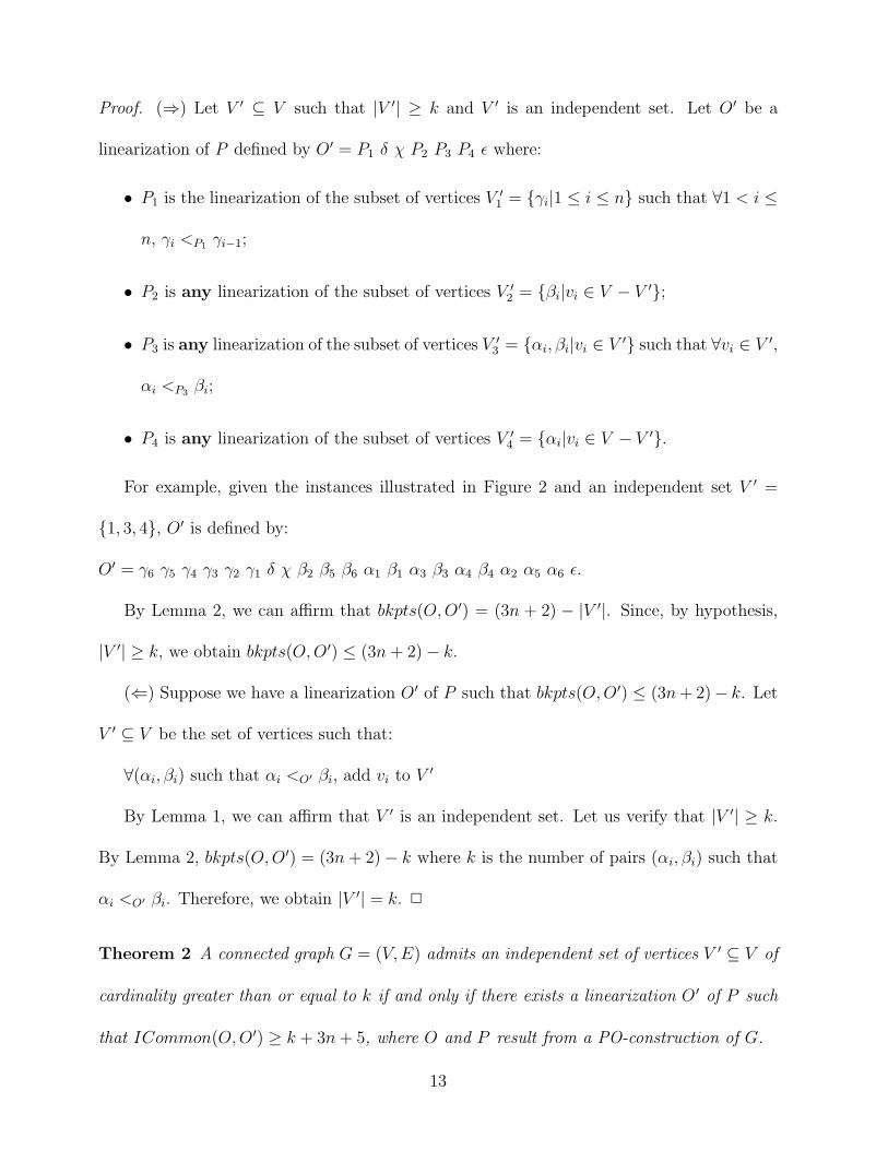
Theorem 2 A connected graph G = (V,E) admits an independent set of vertices V ′ ⊆ V of
cardinality greater than or equal to k if and only if there exists a linearization O ′ of P such
that ICommon(O,O′) ≥ k + 3n + 5, where O and P result from a PO-construction of G.
13
Proof. (⇒) The proof is almost the same as for Theorem 1. Let V ′ ⊆ V such that |V ′| ≥ k
and V ′ is an independent set. Let O′ be a linearization of P defined as in the proof of
Theorem 1 (i.e. O′ = P1 δ χ P2 P3 P4 ε).
By Lemma 4, we can affirm that ICommon(O,O′) = |V ′|+5+3n. Since, by hypothesis,
|V ′| ≥ k, we obtain ICommon(O,O′) ≥ k + 5 + 3n.
(⇐) Suppose we have a linearization O′ of P such that ICommon(O,O′) ≥ k + 5 + 3n.
Let V ′ ⊆ V be the set of vertices such that:
∀(αi, βi) such that αi <O′ βi or βi <O′ αi, add vi to V ′
By Lemma 3, we can affirm that V ′ is an independent set. Let us verify that |V ′| ≥ k.
By Lemma 4, ICommon(O,O′) = k + 5 + 3n where k is the number of pairs (αi, βi) such
that αi <O′ βi or βi <O′ αi. Therefore, we obtain |V ′| = k 2
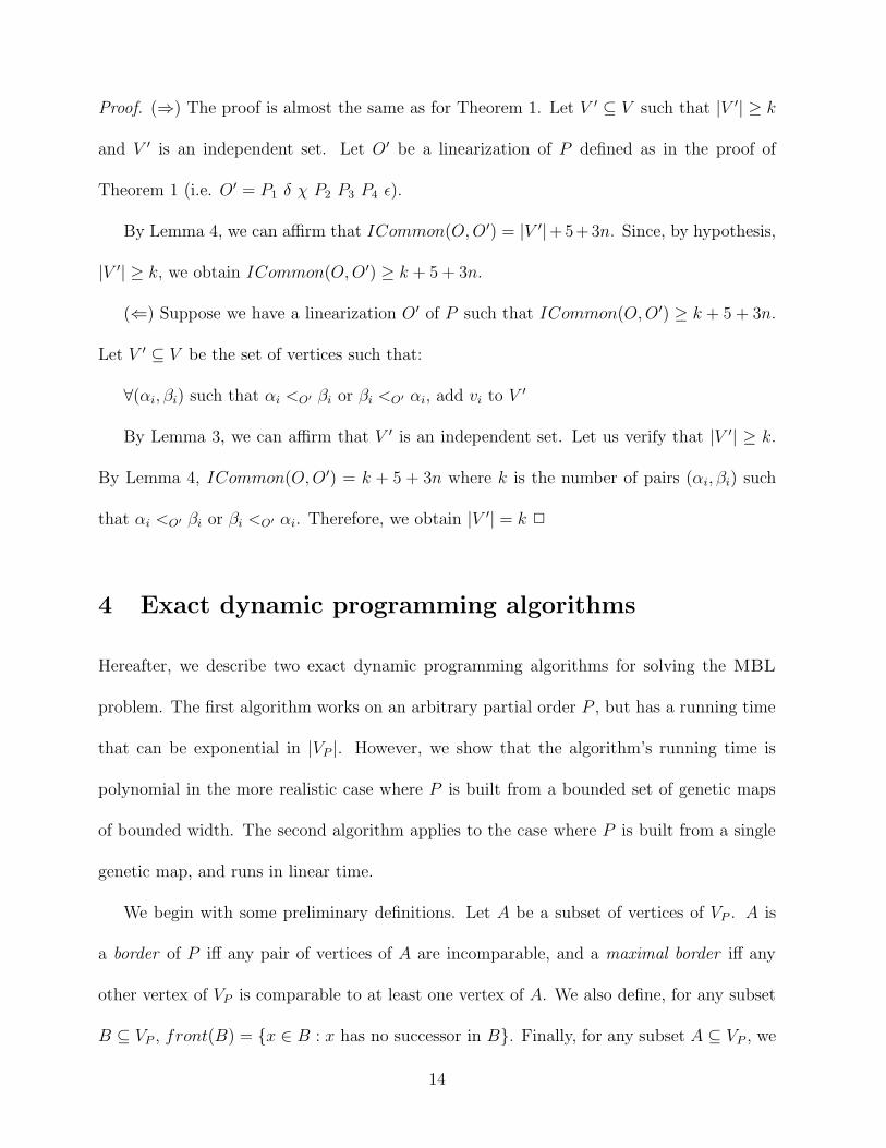
4 Exact dynamic programming algorithms
Hereafter, we describe two exact dynamic programming algorithms for solving the MBL
problem. The first algorithm works on an arbitrary partial order P , but has a running time
that can be exponential in |VP |. However, we show that the algorithm’s running time is
polynomial in the more realistic case where P is built from a bounded set of genetic maps
of bounded width. The second algorithm applies to the case where P is built from a single
genetic map, and runs in linear time.
We begin with some preliminary definitions. Let A be a subset of vertices of VP . A is
a border of P iff any pair of vertices of A are incomparable, and a maximal border iff any
other vertex of VP is comparable to at least one vertex of A. We also define, for any subset
B ⊆ VP , front(B) = {x ∈ B : x has no successor in B}. Finally, for any subset A ⊆ VP , we
14
denote pred(A) = A ∪ {x ∈ VP : ∃y ∈ A s.t. x �P y}.
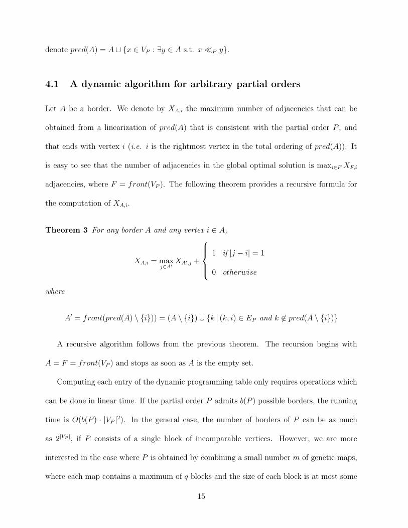
4.1 A dynamic algorithm for arbitrary partial orders
Let A be a border. We denote by XA,i the maximum number of adjacencies that can be
obtained from a linearization of pred(A) that is consistent with the partial order P , and
that ends with vertex i (i.e. i is the rightmost vertex in the total ordering of pred(A)). It
is easy to see that the number of adjacencies in the global optimal solution is maxi∈F XF,i
adjacencies, where F = front(VP ). The following theorem provides a recursive formula for
the computation of XA,i.
Theorem 3 For any border A and any vertex i ∈ A,
XA,i = maxj∈A′
XA′,j +
1 if |j − i| = 1
0 otherwise
where
A′ = front(pred(A) \ {i})) = (A \ {i}) ∪ {k | (k, i) ∈ EP and k 6∈ pred(A \ {i})}
A recursive algorithm follows from the previous theorem. The recursion begins with
A = F = front(VP ) and stops as soon as A is the empty set.
Computing each entry of the dynamic programming table only requires operations which
can be done in linear time. If the partial order P admits b(P ) possible borders, the running
time is O(b(P ) · |VP |2). In the general case, the number of borders of P can be as much
as 2|VP |, if P consists of a single block of incomparable vertices. However, we are more
interested in the case where P is obtained by combining a small number m of genetic maps,
where each map contains a maximum of q blocks and the size of each block is at most some
15
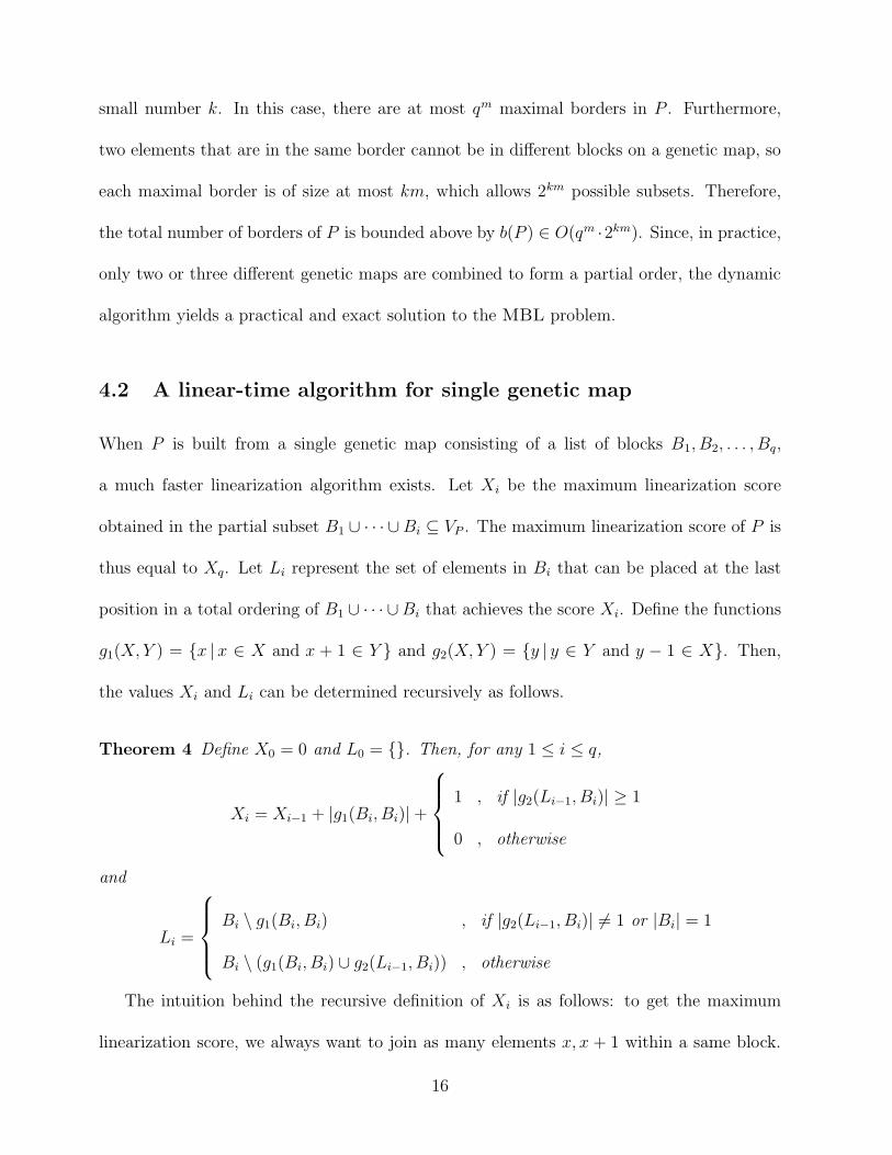
small number k. In this case, there are at most qm maximal borders in P . Furthermore,
two elements that are in the same border cannot be in different blocks on a genetic map, so
each maximal border is of size at most km, which allows 2km possible subsets. Therefore,
the total number of borders of P is bounded above by b(P ) ∈ O(qm ·2km). Since, in practice,
only two or three different genetic maps are combined to form a partial order, the dynamic
algorithm yields a practical and exact solution to the MBL problem.
4.2 A linear-time algorithm for single genetic map
When P is built from a single genetic map consisting of a list of blocks B1, B2, . . . , Bq,
a much faster linearization algorithm exists. Let Xi be the maximum linearization score
obtained in the partial subset B1 ∪ · · · ∪Bi ⊆ VP . The maximum linearization score of P is
thus equal to Xq. Let Li represent the set of elements in Bi that can be placed at the last
position in a total ordering of B1 ∪ · · · ∪Bi that achieves the score Xi. Define the functions
g1(X,Y ) = {x |x ∈ X and x + 1 ∈ Y } and g2(X,Y ) = {y | y ∈ Y and y − 1 ∈ X}. Then,
the values Xi and Li can be determined recursively as follows.
Theorem 4 Define X0 = 0 and L0 = {}. Then, for any 1 ≤ i ≤ q,
Xi = Xi−1 + |g1(Bi, Bi)| +
1 , if |g2(Li−1, Bi)| ≥ 1
0 , otherwise
and
Li =
Bi \ g1(Bi, Bi) , if |g2(Li−1, Bi)| 6= 1 or |Bi| = 1
Bi \ (g1(Bi, Bi) ∪ g2(Li−1, Bi)) , otherwise
The intuition behind the recursive definition of Xi is as follows: to get the maximum
linearization score, we always want to join as many elements x, x + 1 within a same block.
16
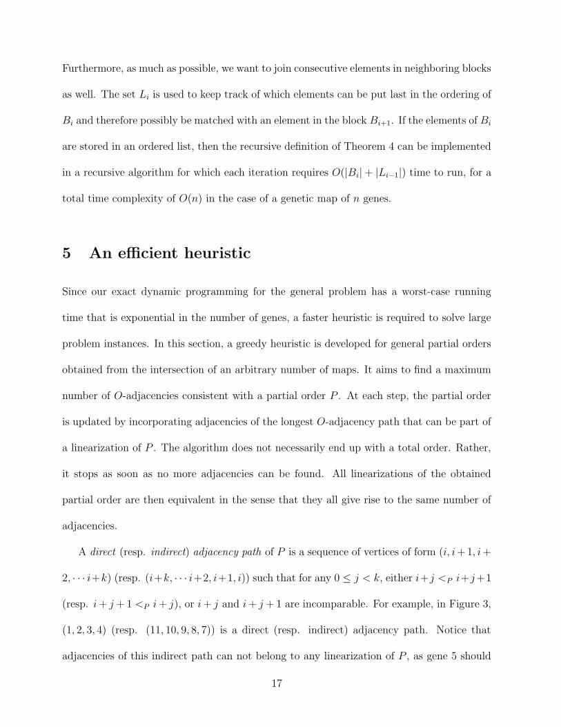
Furthermore, as much as possible, we want to join consecutive elements in neighboring blocks
as well. The set Li is used to keep track of which elements can be put last in the ordering of
Bi and therefore possibly be matched with an element in the block Bi+1. If the elements of Bi
are stored in an ordered list, then the recursive definition of Theorem 4 can be implemented
in a recursive algorithm for which each iteration requires O(|Bi| + |Li−1|) time to run, for a
total time complexity of O(n) in the case of a genetic map of n genes.
5 An efficient heuristic
Since our exact dynamic programming for the general problem has a worst-case running
time that is exponential in the number of genes, a faster heuristic is required to solve large
problem instances. In this section, a greedy heuristic is developed for general partial orders
obtained from the intersection of an arbitrary number of maps. It aims to find a maximum
number of O-adjacencies consistent with a partial order P . At each step, the partial order
is updated by incorporating adjacencies of the longest O-adjacency path that can be part of
a linearization of P . The algorithm does not necessarily end up with a total order. Rather,
it stops as soon as no more adjacencies can be found. All linearizations of the obtained
partial order are then equivalent in the sense that they all give rise to the same number of
adjacencies.
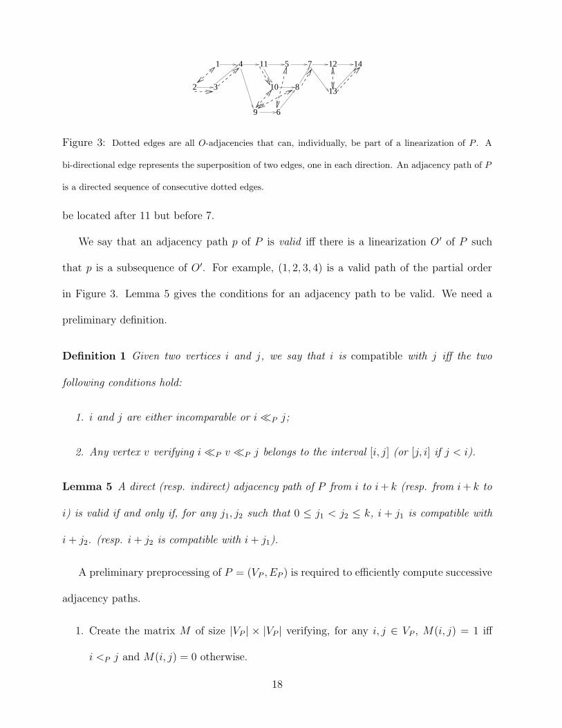
A direct (resp. indirect) adjacency path of P is a sequence of vertices of form (i, i+1, i+
2, · · · i+k) (resp. (i+k, · · · i+2, i+1, i)) such that for any 0 ≤ j < k, either i+j <P i+j+1
(resp. i + j + 1 <P i + j), or i + j and i + j + 1 are incomparable. For example, in Figure 3,
(1, 2, 3, 4) (resp. (11, 10, 9, 8, 7)) is a direct (resp. indirect) adjacency path. Notice that
adjacencies of this indirect path can not belong to any linearization of P , as gene 5 should
17
1 4
10
9
82 3
6
11 5 7 12 14
13
Figure 3: Dotted edges are all O-adjacencies that can, individually, be part of a linearization of P . A
bi-directional edge represents the superposition of two edges, one in each direction. An adjacency path of P
is a directed sequence of consecutive dotted edges.
be located after 11 but before 7.
We say that an adjacency path p of P is valid iff there is a linearization O′ of P such
that p is a subsequence of O′. For example, (1, 2, 3, 4) is a valid path of the partial order
in Figure 3. Lemma 5 gives the conditions for an adjacency path to be valid. We need a
preliminary definition.
Definition 1 Given two vertices i and j, we say that i is compatible with j iff the two
following conditions hold:
1. i and j are either incomparable or i �P j;
2. Any vertex v verifying i �P v �P j belongs to the interval [i, j] (or [j, i] if j < i).
Lemma 5 A direct (resp. indirect) adjacency path of P from i to i + k (resp. from i + k to
i) is valid if and only if, for any j1, j2 such that 0 ≤ j1 < j2 ≤ k, i + j1 is compatible with
i + j2. (resp. i + j2 is compatible with i + j1).
A preliminary preprocessing of P = (VP , EP ) is required to efficiently compute successive
adjacency paths.
1. Create the matrix M of size |VP | × |VP | verifying, for any i, j ∈ VP , M(i, j) = 1 iff
i <P j and M(i, j) = 0 otherwise.
18
Algorithm Find-Valid-Direct-Path (P)
{Compute the list L of all adjacency paths of size 2}
For i = 1 to |V | do
If (i <P i + 1) or (i and i + 1 are incomparable) then
Add (i, i + 1) to L;
End For
k = 2;
{As long as L contains at least two elements, concatenate paths of size k to paths
of size k + 1}
While |L| ≥ 2 do
For j = 1 to |L| do
If Lj+1 and Lj are consecutive paths then
If Lj [1] is compatible with Lj+1[k] then
L′ = Concatenate(Lj , Lj+1);
Add L′ to LNew;
End For
If |LNew| > 0 then L = LNew; Clear(LNew);
k = k + 1;
End While
Return (L1);
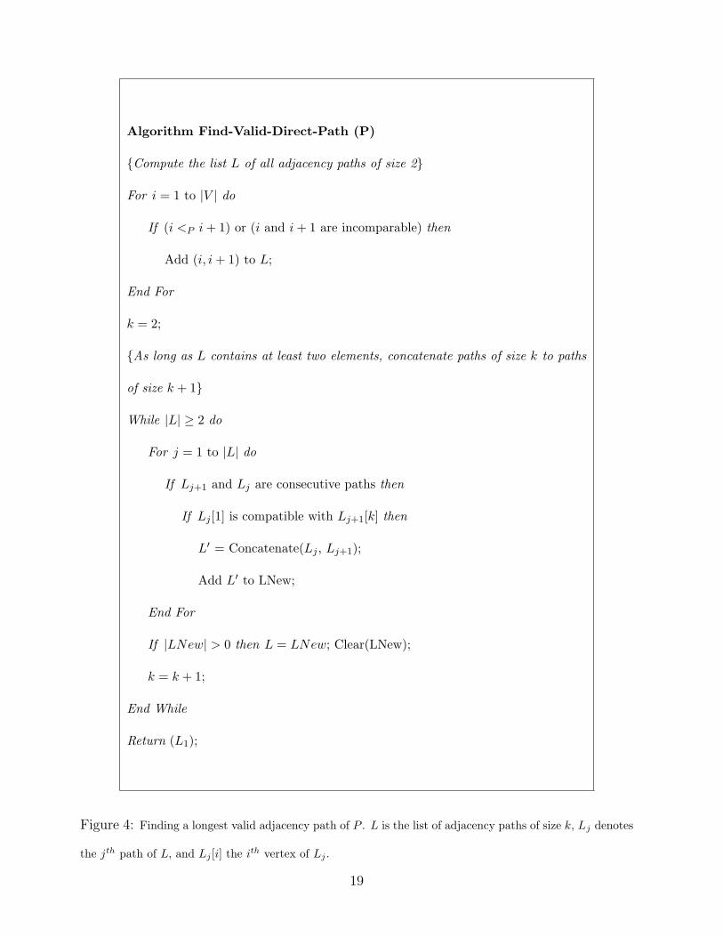
Figure 4: Finding a longest valid adjacency path of P . L is the list of adjacency paths of size k, Lj denotes
the jth path of L, and Lj [i] the ith vertex of Lj .
19
2. Compute the transitive closure of M , that is the matrix M T of size |VP |×|VP | verifying,
for any i, j ∈ VP ,
MT (i, j) =
1 iff i <P j
2 iff i �P j but i ≮P j
0 otherwise
MT is computed from M using the Floyd-Warshall algorithm (Floyd, 1962).
After the preprocessing step, the following Steps 1 and 2 are iterated as long as P contains
an adjacency path.
• Step 1: Find a longest valid direct or indirect adjacency path (see details below).
• Step 2: Incorporate the new adjacencies in MT , and compute the transitive closure
of MT .
Algorithm 4 describes the search of the longest valid direct path. Valid direct paths are
computed beginning with paths of size 2. For a fixed k, any path p = (i, i+1, · · · i+k) of size
k is obtained from a concatenation of two valid consecutive paths p1 = (i, i + 1, · · · i + k− 1)
and p2 = (i+ 1, i+ 2, · · · i+ k) of size k− 1. As p1 and p2 are valid paths, the path p is valid
iff i is compatible with i + k.
The algorithm for valid indirect paths is obtained by replacing the three first lines of
Algorithm 4 by the following:
For i = |V | to 1 doIf (i <P i − 1) or (i and i − 1 are incomparable) then
Add (i, i − 1) to L;
Step 1 consists in running successively both algorithms for direct and indirect paths, and
taking the longest resulting path.
20
Complexity: Computing the transitive closure of the adjacency matrix in the preprocess-
ing phase, as well as in Step 2, is done using the Floyd-Warshall algorithm (Floyd, 1962)
in time complexity O(n3) where n is the number of vertices of the corresponding graph. As
each condition of Algorithm Find-Valid-Path can be checked in constant time and L contains
at most |V | − 1 elements, the time complexity of Step 1 is in O(n). Moreover, Steps 1 and 2
are iterated at most |V | times. Therefore, the worst time complexity of the greedy algorithm
is in O(n4).
6 Experimental results
We first test the efficiency of the heuristic compared to the dynamic programming algorithm
for general partial orders on simulated data, and then illustrate the method on grass maps
obtained from Gramene (http://www.gramene.org/).
Simulated data: We used simulated data to assess the performance of our greedy algo-
rithm. We simulate DAGs of fixed size n that can be represented as a linear expression
involving the operators ‘→’ and ‘,’ where P-adjacent genes are separated by a ‘→’ and
incomparable genes by a ‘,’. Such a representation is similar to the one used in (Lander
et al., 1987; Yap et al., 2003). For example, the DAG in Figure 1.c has the following string
representation:
{2 → 6, 1 → 3 → {4, 5} → 7} → 8 · · · 14 → {9, 15, 16, 17, 21} → {18, 19} → 20
DAGs are generated according to two parameters: the order rate p that determines
the number of ‘,’ in the expression, and the gene distribution rule q corresponding to the
21
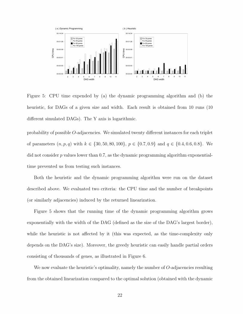
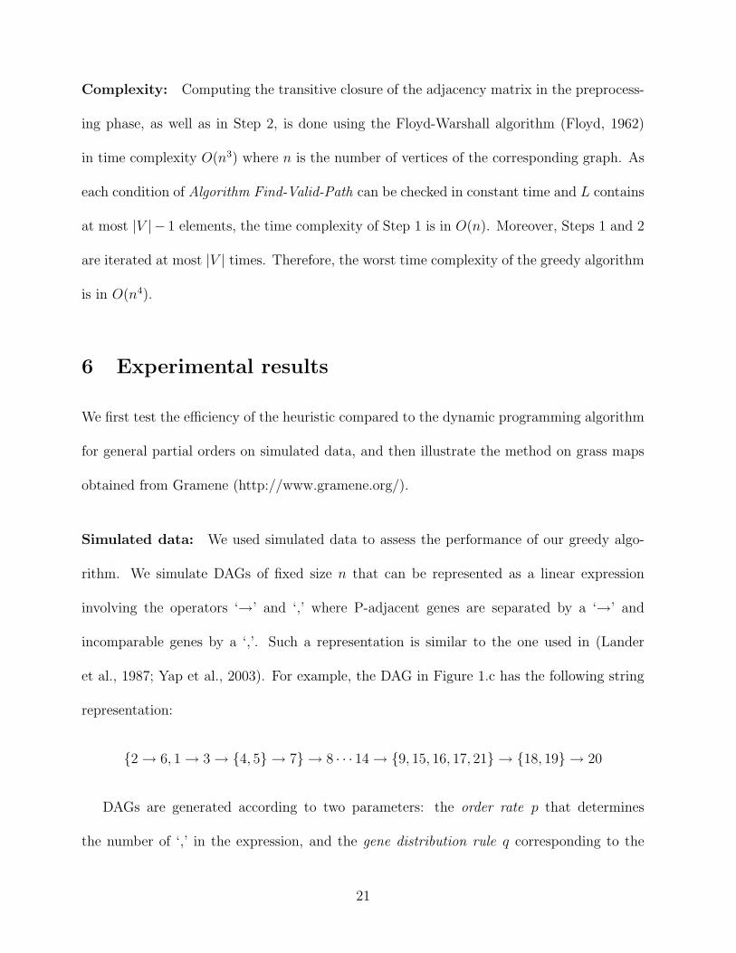
Figure 5: CPU time expended by (a) the dynamic programming algorithm and (b) the
heuristic, for DAGs of a given size and width. Each result is obtained from 10 runs (10
different simulated DAGs). The Y axis is logarithmic.
probability of possible O-adjacencies. We simulated twenty different instances for each triplet
of parameters (n, p, q) with k ∈ {30, 50, 80, 100}, p ∈ {0.7, 0.9} and q ∈ {0.4, 0.6, 0.8}. We
did not consider p values lower than 0.7, as the dynamic programming algorithm exponential-
time prevented us from testing such instances.
Both the heuristic and the dynamic programming algorithm were run on the dataset
described above. We evaluated two criteria: the CPU time and the number of breakpoints
(or similarly adjacencies) induced by the returned linearization.
Figure 5 shows that the running time of the dynamic programming algorithm grows
exponentially with the width of the DAG (defined as the size of the DAG’s largest border),
while the heuristic is not affected by it (this was expected, as the time-complexity only
depends on the DAG’s size). Moreover, the greedy heuristic can easily handle partial orders
consisting of thousands of genes, as illustrated in Figure 6.
We now evaluate the heuristic’s optimality, namely the number of O-adjacencies resulting
from the obtained linearization compared to the optimal solution (obtained with the dynamic
22
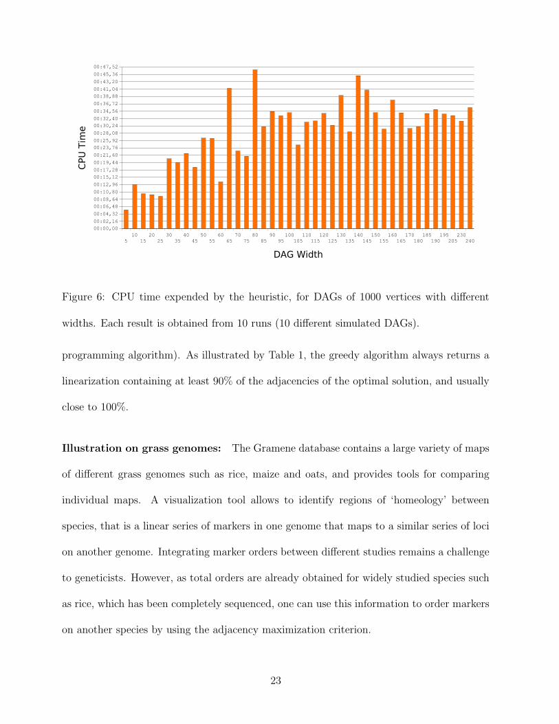
Figure 6: CPU time expended by the heuristic, for DAGs of 1000 vertices with different
widths. Each result is obtained from 10 runs (10 different simulated DAGs).
programming algorithm). As illustrated by Table 1, the greedy algorithm always returns a
linearization containing at least 90% of the adjacencies of the optimal solution, and usually
close to 100%.
Illustration on grass genomes: The Gramene database contains a large variety of maps
of different grass genomes such as rice, maize and oats, and provides tools for comparing
individual maps. A visualization tool allows to identify regions of ‘homeology’ between
species, that is a linear series of markers in one genome that maps to a similar series of loci
on another genome. Integrating marker orders between different studies remains a challenge
to geneticists. However, as total orders are already obtained for widely studied species such
as rice, which has been completely sequenced, one can use this information to order markers
on another species by using the adjacency maximization criterion.
23
DAG Width
2 3 4 5 6 7 8 9 10 11
Gen
ome
size
30 100 100 98,15 97,41 94,33 96,18 93,18 95,54 100 100
50 100 98,04 96,43 97,62 95,25 98,61 100 86,96 95,26 94,94
80 100 98,21 97,90 87,54 96,79 93,89 100 95,83 98,33 100
100 100 98,81 95,65 96,83 89,70 93,95 90,38 95,30 94,63 94,95
Table 1: Percentage of O-adjacencies resulting from the heuristic’s linearization compared to the optimal
solution (obtained with the dynamic programming algorithm). Results are obtained by running the heuristic
and dynamic programming algorithm on 10 different simulated DAGs for a given size and width.
Extracting the linear orders of markers using the Gramene visualization tool remains
unpractical for hundreds of markers, as no automatic tool is provided for this purpose. We
therefore illustrate the method on maps that are small enough to be extracted manually.
Maize has been chosen instead of rice as it has shorter maps, though non-trivial, that can
be represented graphically.
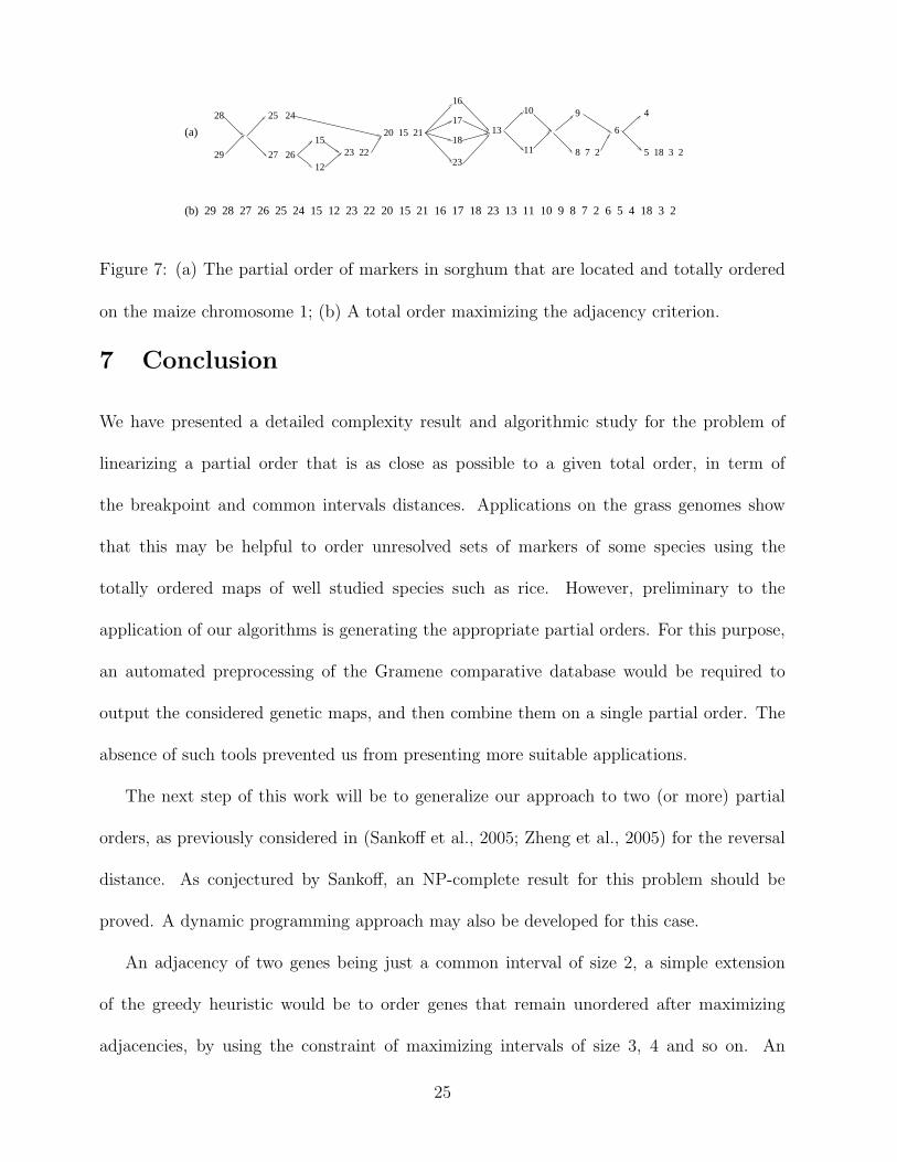
We used the “IBM2 Neighbors 2004” (Polacco and E., 2002) map for chromosomes 5
(Figure 1) and 1 (Figure 7) of maize as a reference, and compared it with the “Paterson
2003” (Bowers et al., 2003) and “Klein 2004” (Menz et al., 2002) maps of the chromosomes
labeled C and LG-01, respectively, of sorghum. We extracted all markers of maize indicated
as having a homolog in one of the databases of sorghum. All are found completely ordered in
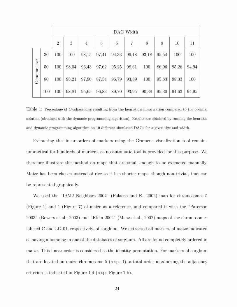
maize. This linear order is considered as the identity permutation. For markers of sorghum
that are located on maize chromosome 5 (resp. 1), a total order maximizing the adjacency
criterion is indicated in Figure 1.d (resp. Figure 7.b).
24
25 24
27 26
20 15 21 15
12
23 22
16
17
18
23
13
11
10 9
8 7 2
6
29
28 4
(a)
(b)
5 18 3 2
29 28 27 26 25 24 15 12 23 22 20 15 21 16 17 18 23 13 11 10 9 8 7 2 6 5 4 18 3 2
Figure 7: (a) The partial order of markers in sorghum that are located and totally ordered
on the maize chromosome 1; (b) A total order maximizing the adjacency criterion.
7 Conclusion
We have presented a detailed complexity result and algorithmic study for the problem of
linearizing a partial order that is as close as possible to a given total order, in term of
the breakpoint and common intervals distances. Applications on the grass genomes show
that this may be helpful to order unresolved sets of markers of some species using the
totally ordered maps of well studied species such as rice. However, preliminary to the
application of our algorithms is generating the appropriate partial orders. For this purpose,
an automated preprocessing of the Gramene comparative database would be required to
output the considered genetic maps, and then combine them on a single partial order. The
absence of such tools prevented us from presenting more suitable applications.
The next step of this work will be to generalize our approach to two (or more) partial
orders, as previously considered in (Sankoff et al., 2005; Zheng et al., 2005) for the reversal
distance. As conjectured by Sankoff, an NP-complete result for this problem should be
proved. A dynamic programming approach may also be developed for this case.
An adjacency of two genes being just a common interval of size 2, a simple extension
of the greedy heuristic would be to order genes that remain unordered after maximizing
adjacencies, by using the constraint of maximizing intervals of size 3, 4 and so on. An
25
efficient heuristic has to be found for the problem of linearizing a partial order considering
the maximal number of common intervals as a criterion.
References
Berard, S., Bergeron, A., and Chauve, C. (2004). Conservation of combinatorial structures
in evolution scenarios. In RECOMB 2004 Satellite meeting on Comparative Genomics,
volume 3388 of LNCS, pages 1 - 14. Springer.
Bergeron, A., Mixtacki, J., and Stoye, J. (2004). Reversal distance without hurdles and
fortresses. In 15th Symposium on Combinatorial Pattern Matching, volume 3109 of
LNCS, pages 388 - 399. Springer.
Blin, G., Chateau, A., Chauve, C., and Gingras, Y. (2006). Inferring positional homologs
with common intervals of sequences. In Fourth Annual RECOMB Satellite meeting on
Comparative Genomics, volume 4205 of LNCS/LNBI, pages 24 - 38.
Blin, G. and Rizzi, R. (2005). Conserved interval distance computation between non-
trivial genomes. In Proc. 11th International Computing and Combinatorics Conference
(COCOON’05), volume 3595 of LNCS, pages 22–31.
Bourque, G., Yacef, Y., and El-Mabrouk, N. (2005a). Maximizing synteny blocks to iden-
tify ancestral homologs. In Third Annual RECOMB Satellite meeting on Comparative
Genomics, volume 3678 of LNCS/LNBI, pages 21 - 34.
Bourque, G., Zdobnov, E., Bork, P., Pavzner, P., and Tesler, G. (2005b). Comparative ar-
chitectures of mammalian and chicken genomes reveal highly variable rates of genomic
rearrangements across different lineages. Genome Research, 15:98- 110.
26
Bowers, J., Abbey, C., Anderson, A., Chang, C., Draye, X., Hoppe, A., Jessup, R., Lemke,
C., Lennington, J., Li, Z., Lin, Y., Liu, S., Luo, L., Marler, B., Ming, R., Mitchell, S.,
Qiang, D., Reischmann, K., Schulze, S., Skinner, D., Wang, Y., Kresovich, S., Schertz,
K., and Paterson., A. (2003). A high-density genetic recombination map of sequence-
tagged sites for Sorghum, as a framework for comparative structural and evolutionary
genomics of tropical grains and grasses. Genetics, 165:367-386.
El-Mabrouk, N. (2000). Sorting signed permutations by reversals and insertions/deletions
of contiguous segments. Journal of Discrete Algorithms, 1(1):105-122.
Figeac, M. and Varre, J. (2004). Sorting by reversals with common intervals. In WABI,
volume 3240 of LNBI, pages 26 - 37. Springer-Verlag.
Floyd, R. W. (1962). Algorithm 97: Shortest path. Communications of the ACM, 5(6):345.
Garey, M. and Johnson, D. (1979). Computers and Intractability: A Guide to the Theory
of NP-Completeness. W. H. Freeman and Company.
Hannenhalli, S. and Pevzner, P. A. (1999). Transforming cabbage into turnip (polynomial
algorithm for sorting signed permutations by reversals). Journal of the ACM, 48:1–27.
Jackson, B., Aluru, S., and Schnable, P. (2005). Consensus genetic maps: a graph the-
ory approach. In IEEE Computational Systems Bioinformatics Conference (CSB’05),
pages 35- 43.
Lander, S., Green, P., Abrahamson, J., and amd M.J Daly et al., A. B. (1987). MAP-
MAKER: an interactive computer package for constructing primary genetic linkage
maps of experimental and natural populations. Genomics, 1:174 - 181.
Menz, M., Klein, R., Mullet, J., Obert, J., Unruh, N., and Klein, P. (2002). A High-
27
Density Genetic Map of Sorghum Bicolor (L.) Moench Based on 2926 Aflp, Rflp and
Ssr Markers. Plant Molecular Biology, 48:483–99.
Pevzner, P. and Tesler, G. (2003). Human and mouse genomic sequences reveal extensive
breakpoint reuse in mammalian evolution. Proc. Natl. Acad. Sci. USA, 100:7672 - 7677.
Polacco, M. and E., J. C. (2002). IBM neighbors: a consensus GeneticMap.
Sankoff, D., Zheng, C., and Lenert, A. (2005). Reversals of fortune. Proceedings of the 3rd
RECOMB Comparative Genomics Satellite Workshop, 3678:131–141.
Tang, J. and Moret, B. (2003). Phylogenetic reconstruction from gene rearrangement
data with unequal gene contents. In Lecture Notes in Computer Science, volume 2748
of WADS’03, pages 37- 46. Springer Verlag.
Yap, I., Schneider, D., Kleinberg, J., Matthews, D., Cartinhour, S., and McCouch, S. R.
(2003). A graph-theoretic approach to comparing and integrating genetic, physical and
sequence-based maps. Genetics, 165:2235- 2247.
Zheng, C., Lenert, A., and Sankoff, D. (2005). Reversal distance for partially ordered
genomes. Bioinformatics, 21, Suppl 1:i502–i508.
28