Gene Flow, Genetic Drift

Natural Selection

Lecture 9

Spring 2013

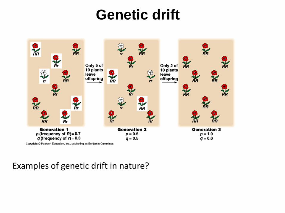
Genetic drift

Examples of genetic drift in nature?

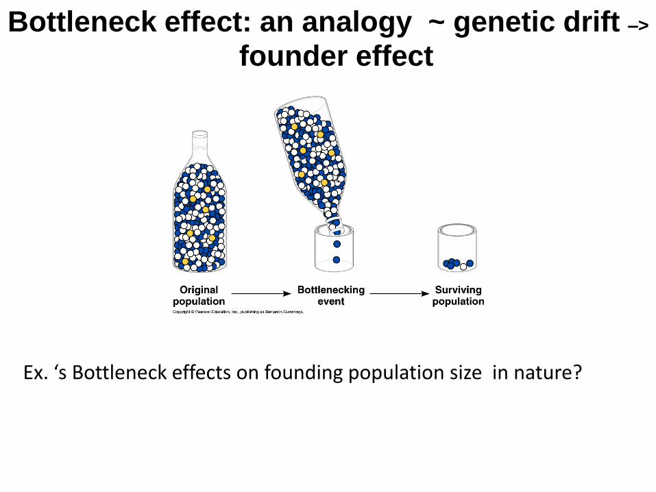
Bottleneck effect: an analogy ~ genetic drift –>

founder effect

Ex. ‘s Bottleneck effects on founding population size in nature?

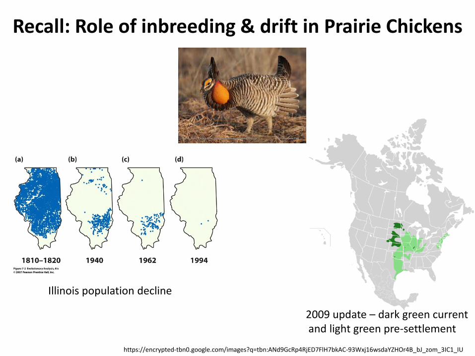
Recall: Role of inbreeding & drift in Prairie Chickens

https://encrypted-tbn0.google.com/images?q=tbn:ANd9GcRp4RjED7FlH7bkAC-93Wxj16wsdaYZHOr4B_bJ_zom_3IC1_IU

2009 update – dark green current and light green pre-settlement

Illinois population decline

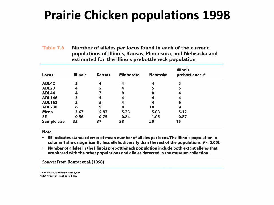
Prairie Chicken populations 1998

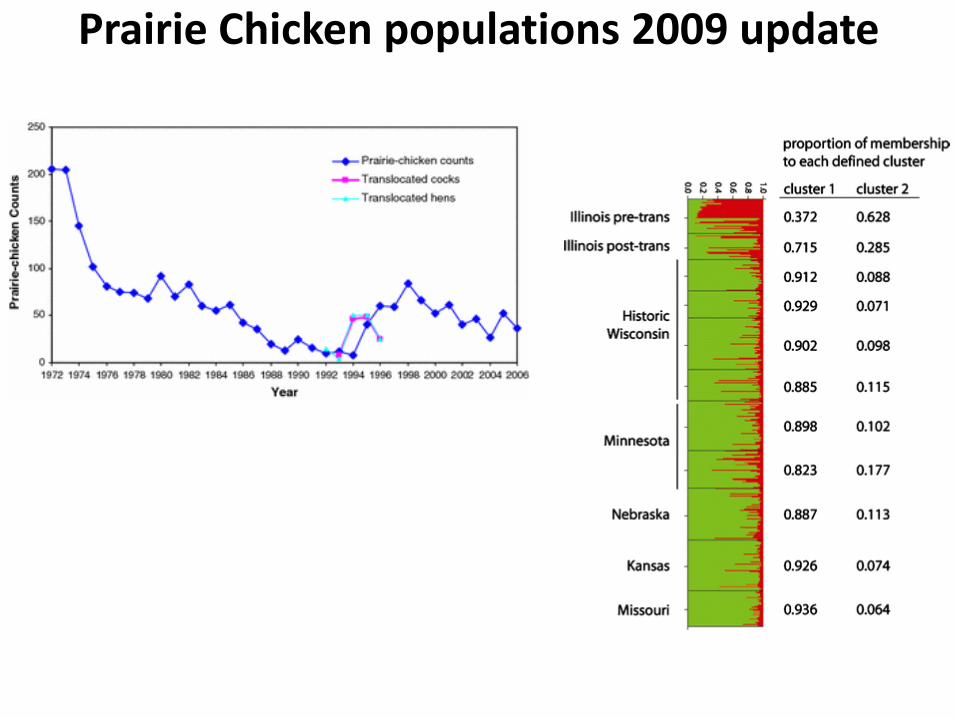
Prairie Chicken populations 2009 update

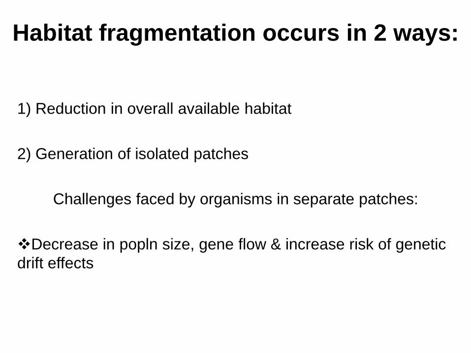
Habitat fragmentation occurs in 2 ways:

1) Reduction in overall available habitat

2) Generation of isolated patches

Challenges faced by organisms in separate patches:

Decrease in popln size, gene flow & increase risk of genetic

drift effects

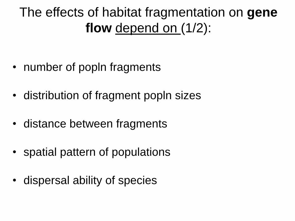
The effects of habitat fragmentation on gene

flow depend on (1/2):

• number of popln fragments

• distribution of fragment popln sizes

• distance between fragments

• spatial pattern of populations

• dispersal ability of species

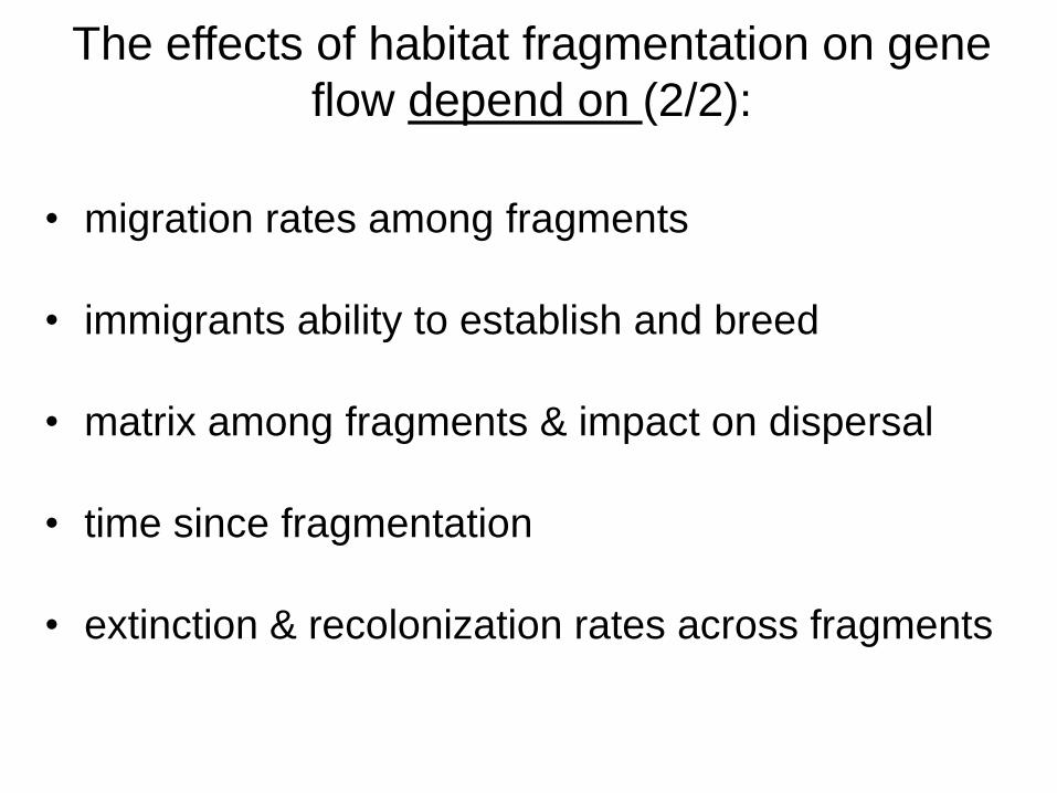
The effects of habitat fragmentation on gene

flow depend on (2/2):

• migration rates among fragments

• immigrants ability to establish and breed

• matrix among fragments & impact on dispersal

• time since fragmentation

• extinction & recolonization rates across fragments

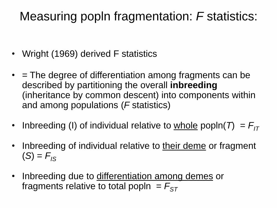
Measuring popln fragmentation: F statistics:

• Wright (1969) derived F statistics

• = The degree of differentiation among fragments can be described by partitioning the overall inbreeding (inheritance by common descent) into components within and among populations (F statistics)

• Inbreeding (I) of individual relative to whole popln(T) = FIT

• Inbreeding of individual relative to their deme or fragment (S) = FIS

• Inbreeding due to differentiation among demes or fragments relative to total popln = FST

Measuring popln fragmentation: F statistics:

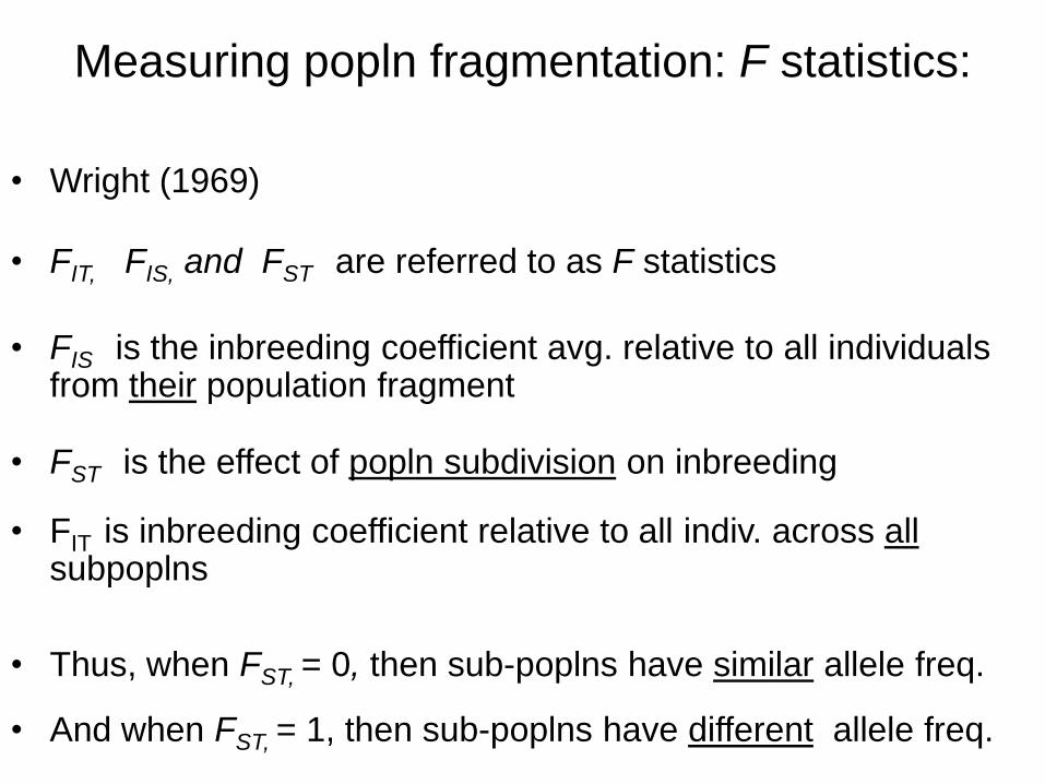
• Wright (1969)

• FIT, FIS, and FST are referred to as F statistics

• FIS is the inbreeding coefficient avg. relative to all individuals from their population fragment

• FST is the effect of popln subdivision on inbreeding

• FIT is inbreeding coefficient relative to all indiv. across all subpoplns

• Thus, when FST, = 0, then sub-poplns have similar allele freq.

• And when FST, = 1, then sub-poplns have different allele freq.

Calculating : F statistics:

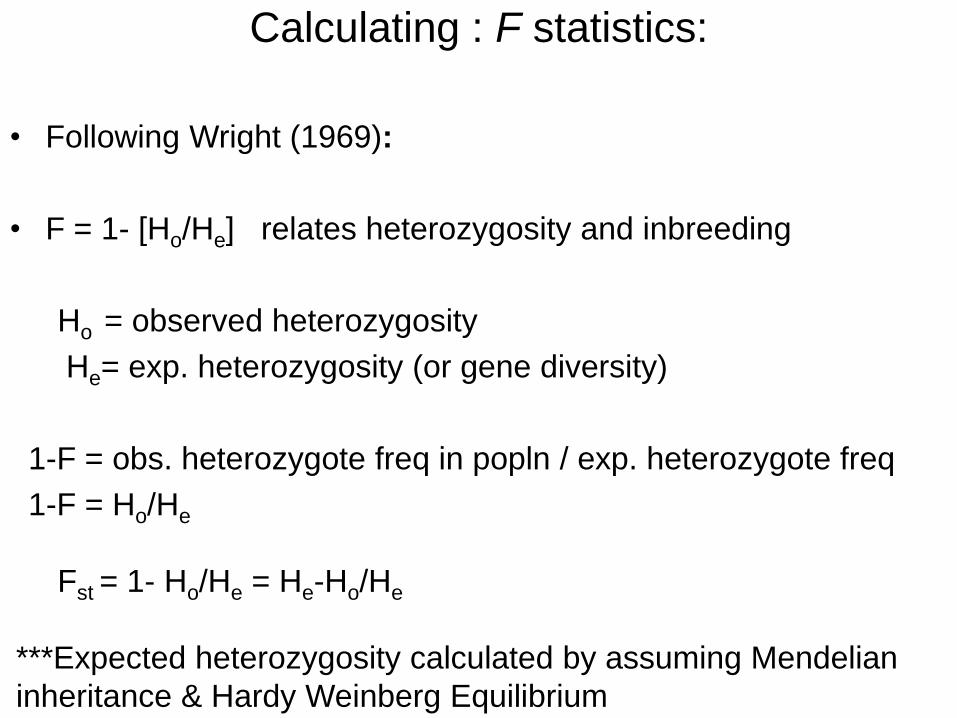
• Following Wright (1969):

• F = 1- [Ho/He] relates heterozygosity and inbreeding

Ho = observed heterozygosity

He= exp. heterozygosity (or gene diversity)

1-F = obs. heterozygote freq in popln / exp. heterozygote freq

1-F = Ho/He

Fst = 1- Ho/He = He-Ho/He

***Expected heterozygosity calculated by assuming Mendelian

inheritance & Hardy Weinberg Equilibrium

Calculating : F statistics:

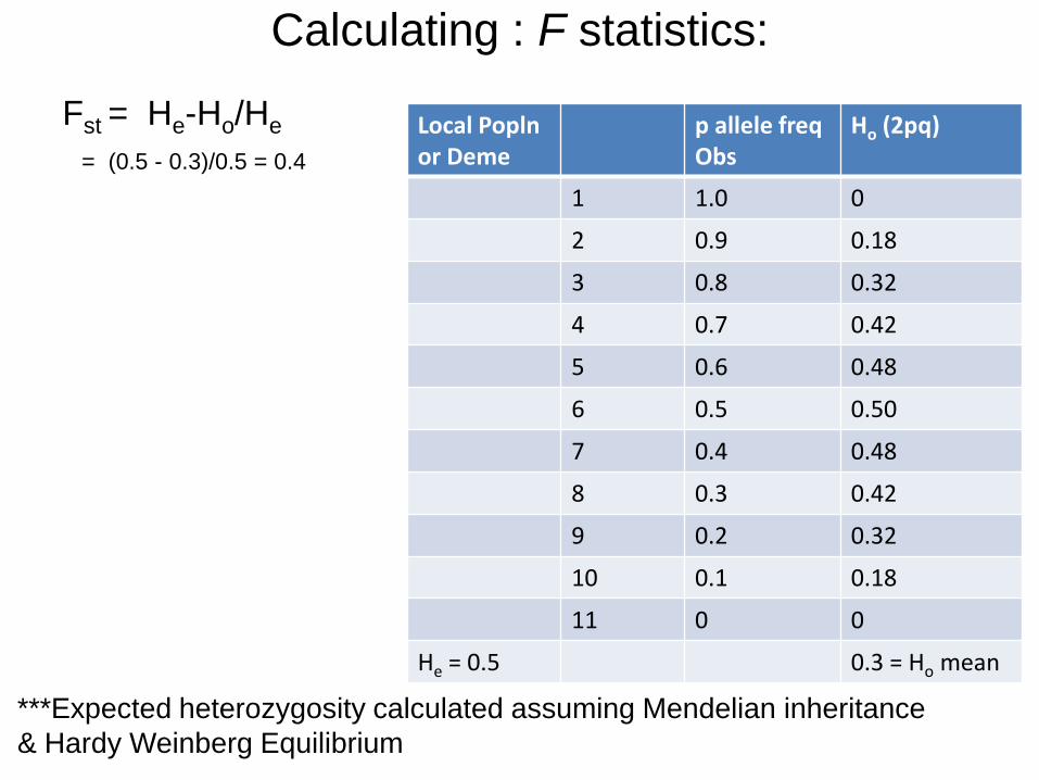
Fst = He-Ho/He

= (0.5 - 0.3)/0.5 = 0.4

Local Popln or Deme

p allele freq Obs

Ho (2pq)

1 1.0 0

2 0.9 0.18

3 0.8 0.32

4 0.7 0.42

5 0.6 0.48

6 0.5 0.50

7 0.4 0.48

8 0.3 0.42

9 0.2 0.32

10 0.1 0.18

11 0 0

He = 0.5 0.3 = Ho mean

***Expected heterozygosity calculated assuming Mendelian inheritance

& Hardy Weinberg Equilibrium

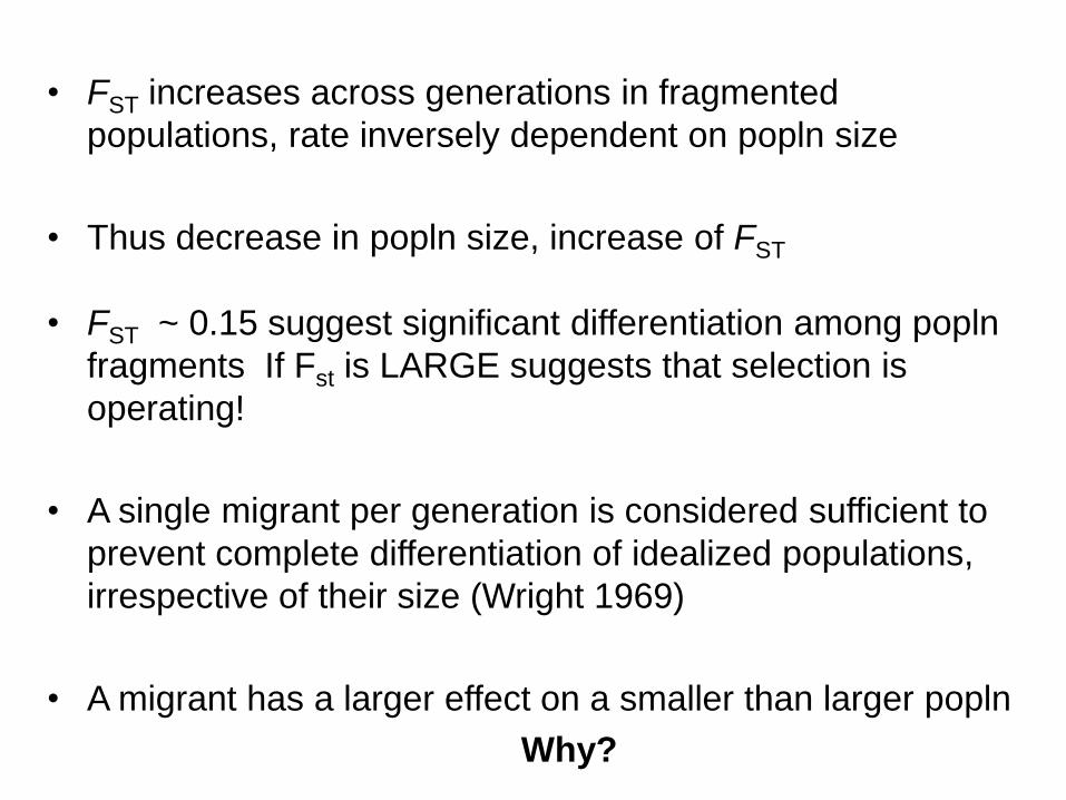
• FST increases across generations in fragmented

populations, rate inversely dependent on popln size

• Thus decrease in popln size, increase of FST

• FST ~ 0.15 suggest significant differentiation among popln

fragments If Fst is LARGE suggests that selection is

operating!

• A single migrant per generation is considered sufficient to

prevent complete differentiation of idealized populations,

irrespective of their size (Wright 1969)

• A migrant has a larger effect on a smaller than larger popln

Why?

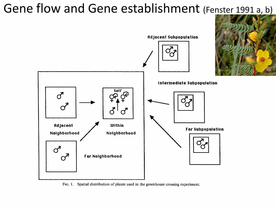
Gene flow and Gene establishment (Fenster 1991 a, b)

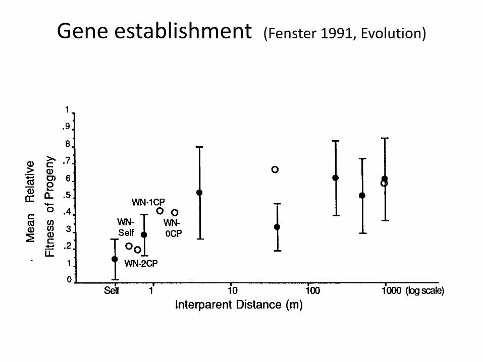
Gene establishment (Fenster 1991, Evolution)

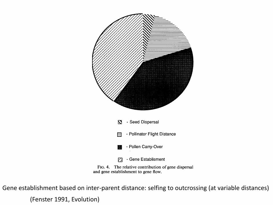
(Fenster 1991, Evolution)

Gene establishment based on inter-parent distance: selfing to outcrossing (at variable distances)

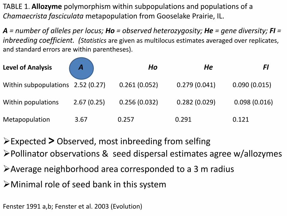
TABLE 1. Allozyme polymorphism within subpopulations and populations of a Chamaecrista fasciculata metapopulation from Gooselake Prairie, IL.

A = number of alleles per locus; Ho = observed heterozygosity; He = gene diversity; FI = inbreeding coefficient. (Statistics are given as multilocus estimates averaged over replicates, and standard errors are within parentheses).

Level of Analysis A Ho He FI Within subpopulations 2.52 (0.27) 0.261 (0.052) 0.279 (0.041) 0.090 (0.015) Within populations 2.67 (0.25) 0.256 (0.032) 0.282 (0.029) 0.098 (0.016) Metapopulation 3.67 0.257 0.291 0.121

Expected > Observed, most inbreeding from selfing

Pollinator observations & seed dispersal estimates agree w/allozymes

Average neighborhood area corresponded to a 3 m radius

Minimal role of seed bank in this system

Fenster 1991 a,b; Fenster et al. 2003 (Evolution)

Gene flow can be estimated from the degree of genetic

differentiation among populations (Fst).

Gene flow among fragmented populations is related to

dispersal ability

Gene Flow and Dispersal Ability

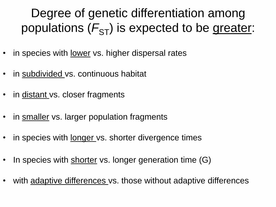
Degree of genetic differentiation among

populations (FST) is expected to be greater:

• in species with lower vs. higher dispersal rates

• in subdivided vs. continuous habitat

• in distant vs. closer fragments

• in smaller vs. larger population fragments

• in species with longer vs. shorter divergence times

• In species with shorter vs. longer generation time (G)

• with adaptive differences vs. those without adaptive differences

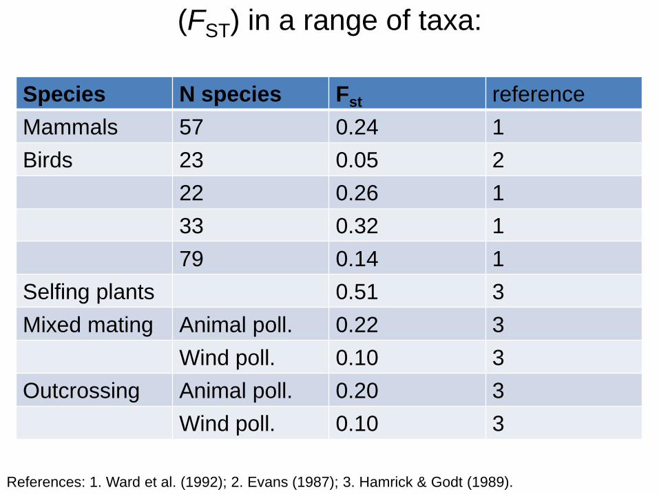
(FST) in a range of taxa:

Species N species Fst reference

Mammals 57 0.24 1

Birds 23 0.05 2

22 0.26 1

33 0.32 1

79 0.14 1

Selfing plants 0.51 3

Mixed mating Animal poll. 0.22 3

Wind poll. 0.10 3

Outcrossing Animal poll. 0.20 3

Wind poll. 0.10 3

References: 1. Ward et al. (1992); 2. Evans (1987); 3. Hamrick & Godt (1989).

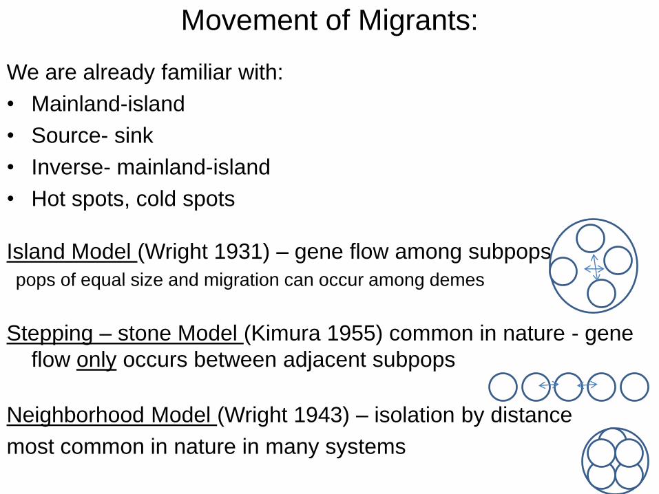
Movement of Migrants:

We are already familiar with:

• Mainland-island

• Source- sink

• Inverse- mainland-island

• Hot spots, cold spots

Island Model (Wright 1931) – gene flow among subpops

pops of equal size and migration can occur among demes

Stepping – stone Model (Kimura 1955) common in nature - gene

flow only occurs between adjacent subpops

Neighborhood Model (Wright 1943) – isolation by distance

most common in nature in many systems

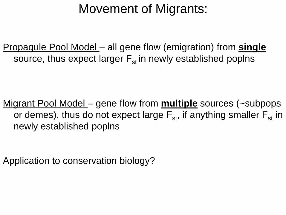
Movement of Migrants:

Propagule Pool Model – all gene flow (emigration) from single

source, thus expect larger Fst in newly established poplns

Migrant Pool Model – gene flow from multiple sources (~subpops

or demes), thus do not expect large Fst, if anything smaller Fst in

newly established poplns

Application to conservation biology?

Natural Selection

Four principles on Natural Selection:

1)

2)

3)

4)

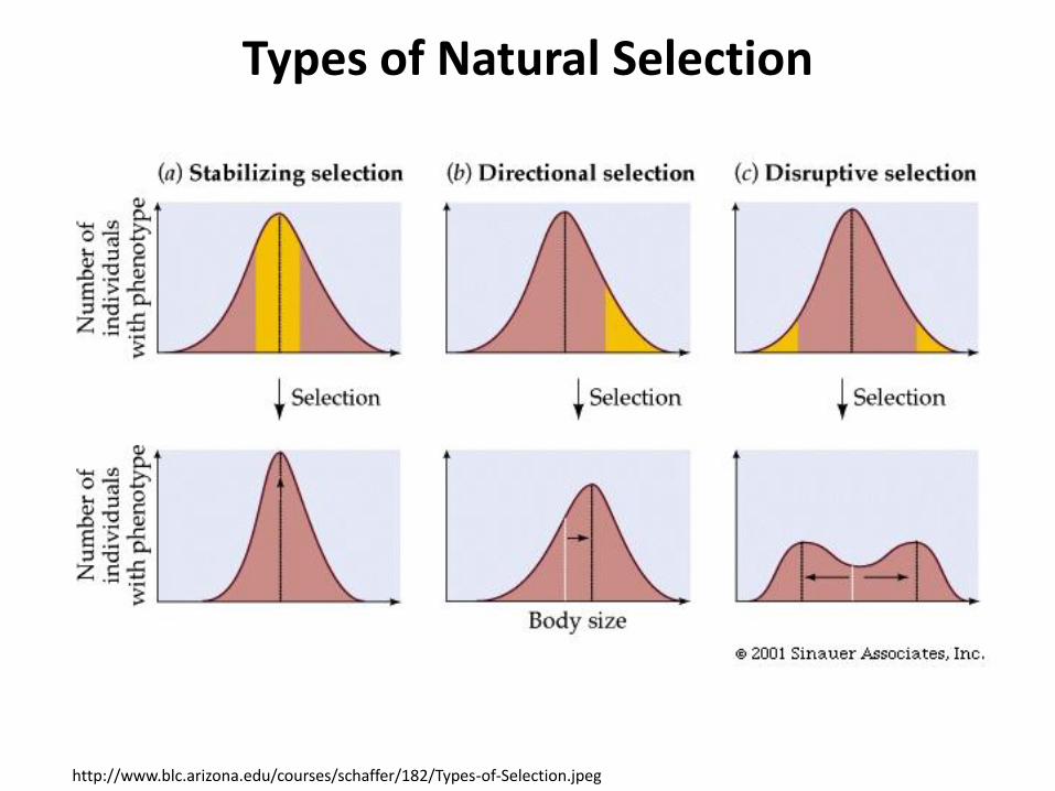
Types of Natural Selection

http://www.blc.arizona.edu/courses/schaffer/182/Types-of-Selection.jpeg

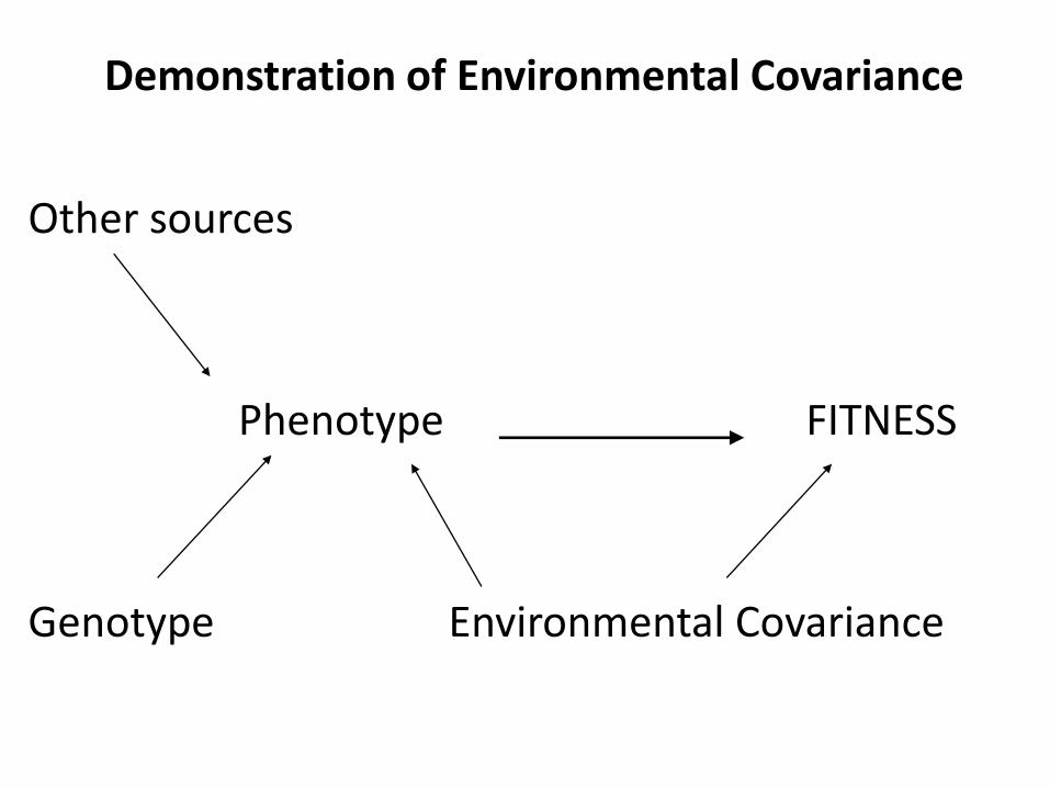
Demonstration of Environmental Covariance

Other sources

Phenotype FITNESS

Genotype Environmental Covariance

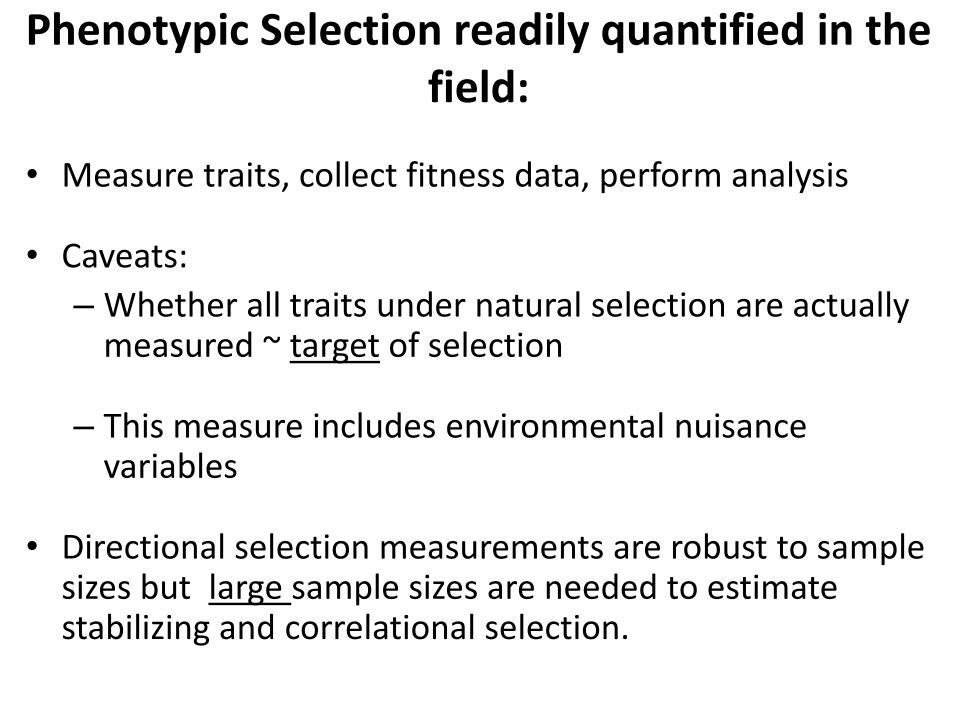
Phenotypic Selection readily quantified in the field:

• Measure traits, collect fitness data, perform analysis

• Caveats:

– Whether all traits under natural selection are actually measured ~ target of selection

– This measure includes environmental nuisance variables

• Directional selection measurements are robust to sample sizes but large sample sizes are needed to estimate stabilizing and correlational selection.

Parental trait value

Off

spri

ng

tra

it v

alu

e

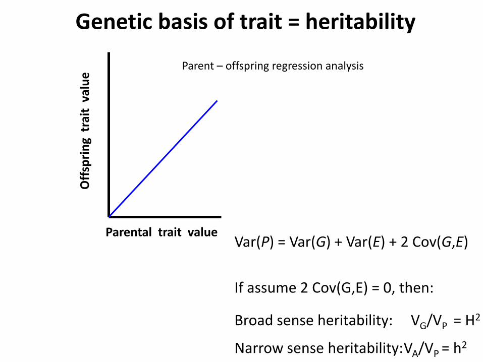
Genetic basis of trait = heritability

Parent – offspring regression analysis

Var(P) = Var(G) + Var(E) + 2 Cov(G,E)

If assume 2 Cov(G,E) = 0, then:

Broad sense heritability: VG/VP = H2

Narrow sense heritability: VA/VP = h2

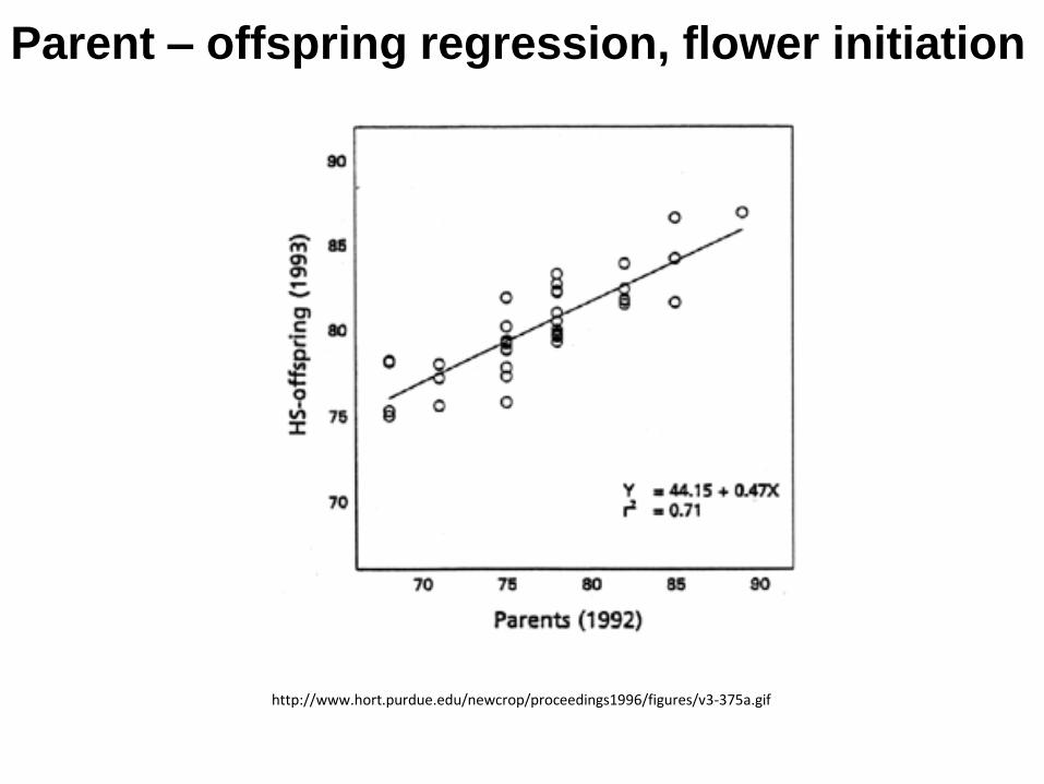
http://www.hort.purdue.edu/newcrop/proceedings1996/figures/v3-375a.gif

Parent – offspring regression, flower initiation

w,

rela

tive

fit

ne

ss

x, trait

x

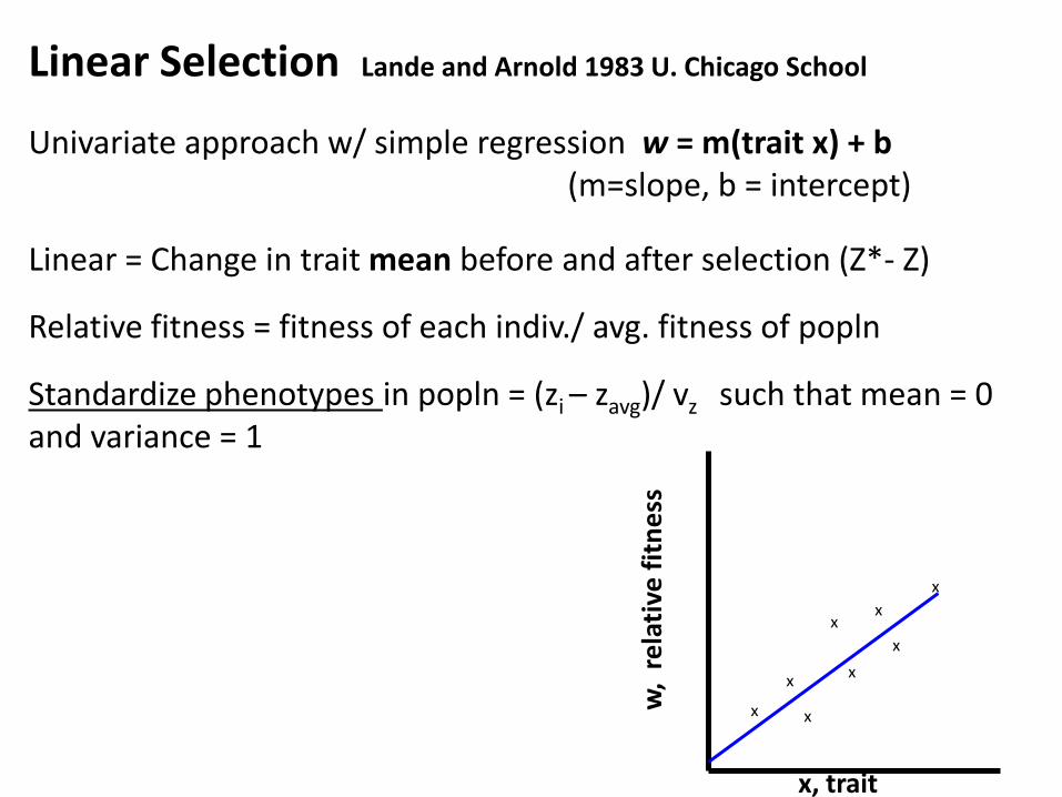
Linear Selection Lande and Arnold 1983 U. Chicago School

Univariate approach w/ simple regression w = m(trait x) + b (m=slope, b = intercept)

Linear = Change in trait mean before and after selection (Z*- Z)

Relative fitness = fitness of each indiv./ avg. fitness of popln

Standardize phenotypes in popln = (zi – zavg)/ vz such that mean = 0 and variance = 1

x

x

x x

x x

x

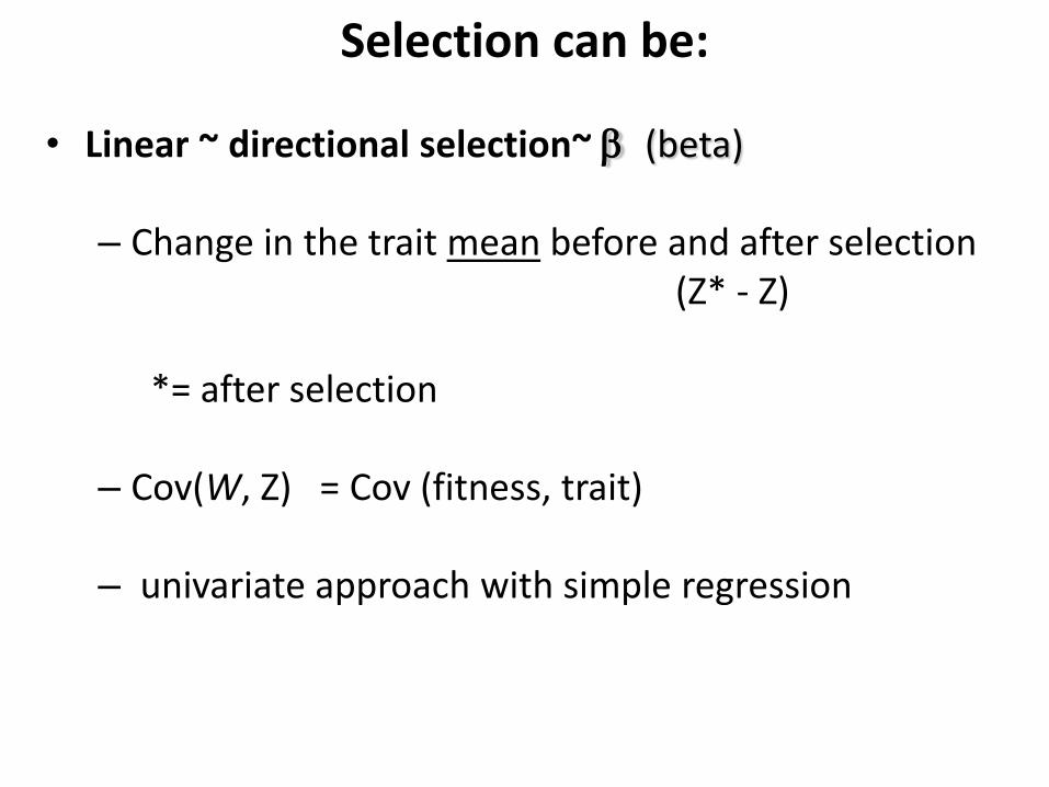
Selection can be:

• Linear ~ directional selection~ b (beta) – Change in the trait mean before and after selection (Z* - Z)

*= after selection

– Cov(W, Z) = Cov (fitness, trait)

– univariate approach with simple regression

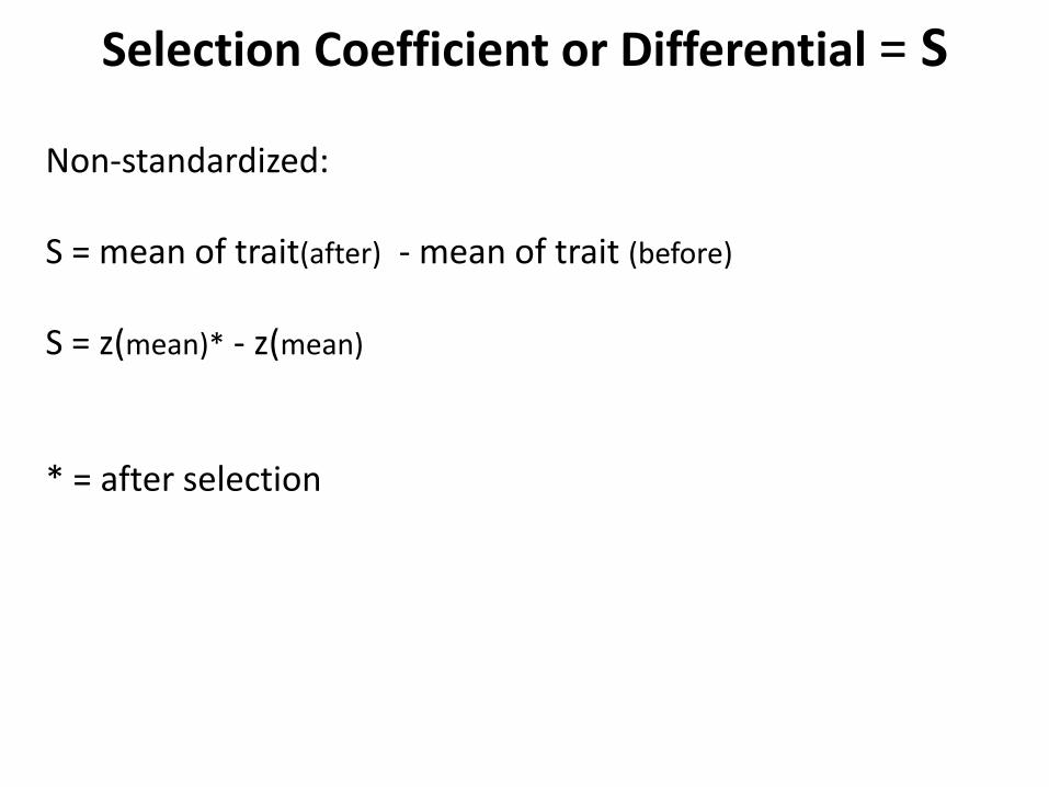
Selection Coefficient or Differential = S

Non-standardized: S = mean of trait(after) - mean of trait (before)

S = z(mean)* - z(mean)

* = after selection

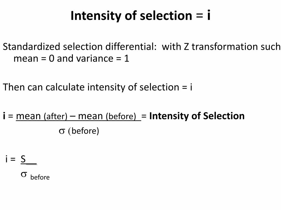
Intensity of selection = i

Standardized selection differential: with Z transformation such mean = 0 and variance = 1

Then can calculate intensity of selection = i

i = mean (after) – mean (before) = Intensity of Selection

s (before)

i = S__

s before

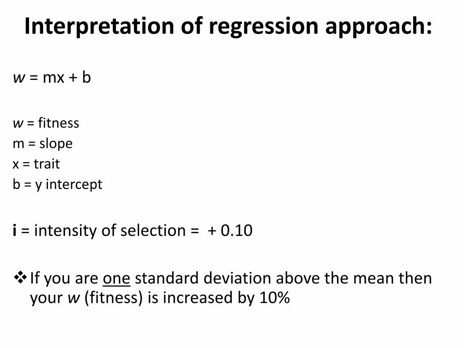
Interpretation of regression approach:

w = mx + b

w = fitness

m = slope

x = trait

b = y intercept

i = intensity of selection = + 0.10

If you are one standard deviation above the mean then your w (fitness) is increased by 10%

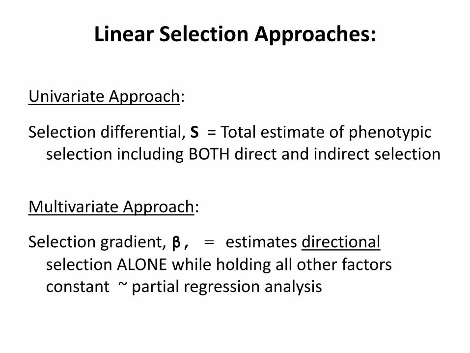
Linear Selection Approaches:

Univariate Approach:

Selection differential, S = Total estimate of phenotypic selection including BOTH direct and indirect selection

Multivariate Approach:

Selection gradient, β, = estimates directional selection ALONE while holding all other factors constant ~ partial regression analysis

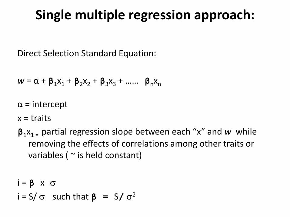
Single multiple regression approach:

Direct Selection Standard Equation:

w = α + β1x1 + β2x2 + β3x3 + …… βnxn

α = intercept

x = traits

β1x1 = partial regression slope between each “x” and w while removing the effects of correlations among other traits or variables ( ~ is held constant)

i = β x s

i = S/ s such that β = S/ s2

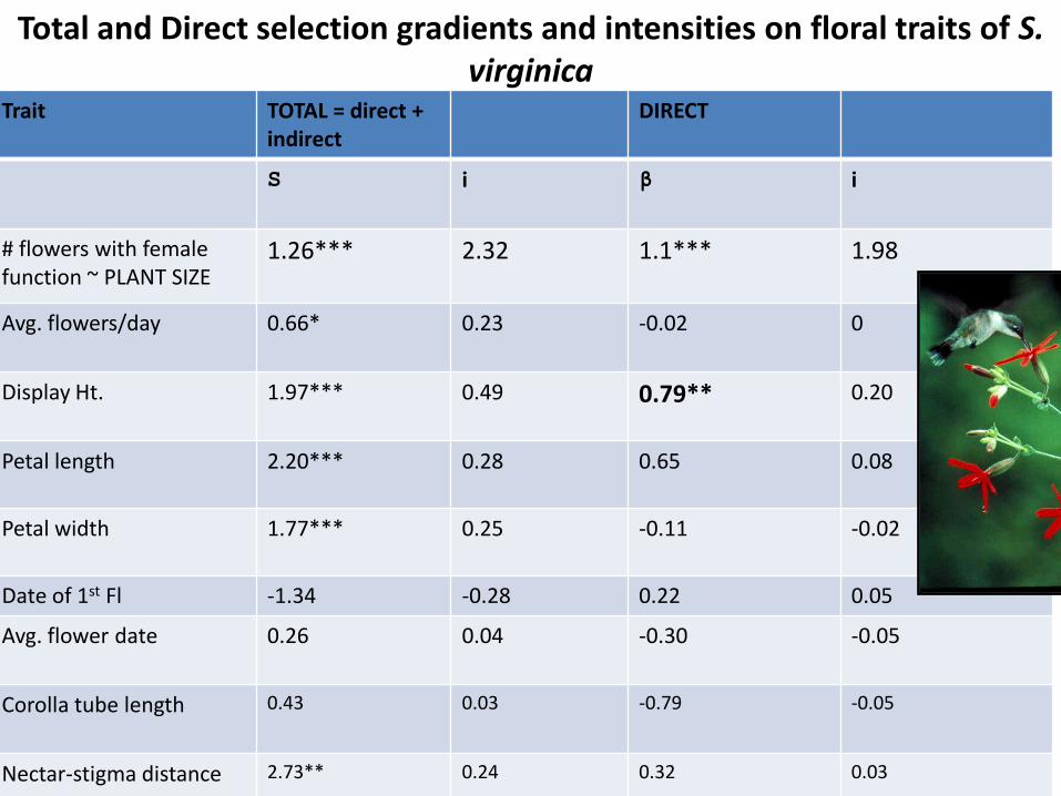
Total and Direct selection gradients and intensities on floral traits of S. virginica

Trait

TOTAL = direct + indirect

DIRECT

S

i β

i

# flowers with female function ~ PLANT SIZE

1.26***

2.32

1.1***

1.98

Avg. flowers/day 0.66*

0.23 -0.02 0

Display Ht. 1.97*** 0.49 0.79** 0.20

Petal length

2.20*** 0.28 0.65 0.08

Petal width

1.77*** 0.25 -0.11 -0.02

Date of 1st Fl -1.34 -0.28 0.22 0.05

Avg. flower date 0.26 0.04 -0.30 -0.05

Corolla tube length 0.43 0.03 -0.79 -0.05

Nectar-stigma distance 2.73** 0.24 0.32 0.03

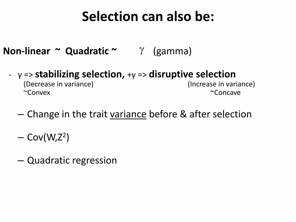
Selection can also be:

Non-linear ~ Quadratic ~ (gamma)

- γ => stabilizing selection, +γ => disruptive selection

(Decrease in variance) (Increase in variance) ~Convex ~Concave

– Change in the trait variance before & after selection

– Cov(W,Z2)

– Quadratic regression

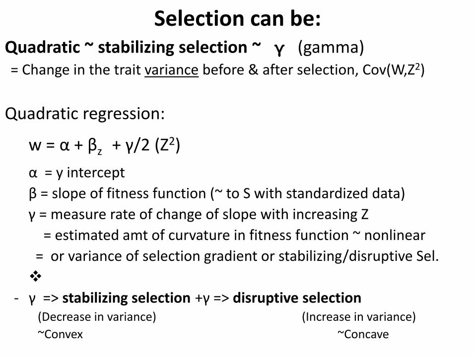
Selection can be: Quadratic ~ stabilizing selection ~ γ (gamma) = Change in the trait variance before & after selection, Cov(W,Z2)

Quadratic regression:

w = α + βz + γ/2 (Z2)

α = y intercept

β = slope of fitness function (~ to S with standardized data)

γ = measure rate of change of slope with increasing Z

= estimated amt of curvature in fitness function ~ nonlinear

= or variance of selection gradient or stabilizing/disruptive Sel.

- γ => stabilizing selection +γ => disruptive selection (Decrease in variance) (Increase in variance)

~Convex ~Concave

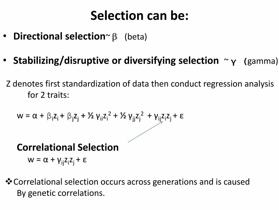
Selection can be:

• Directional selection~ b (beta)

• Stabilizing/disruptive or diversifying selection ~ γ (gamma)

Z denotes first standardization of data then conduct regression analysis for 2 traits:

w = α + βizi + βjzj + ½ γiizi2 + ½ γjjzj

2 + γijzizj + ε

Correlational Selection w = α + γijzizj

+ ε

Correlational selection occurs across generations and is caused By genetic correlations.

Correlational Selection

• Selection favors combinations of traits over single traits alone.

• Traits become functionally integrated with each other.

• Promotes genetic integration or coupling.

If considering only two traits:

• Directional selection – trait means shift before & after selection

• Stabilizing/diversifying or disruptive selection – variance of traits shift before and after selection as well as the correlation between two traits (~correlational)

Thus need to consider 3 forms of selection utilizing multiple regression techniques.

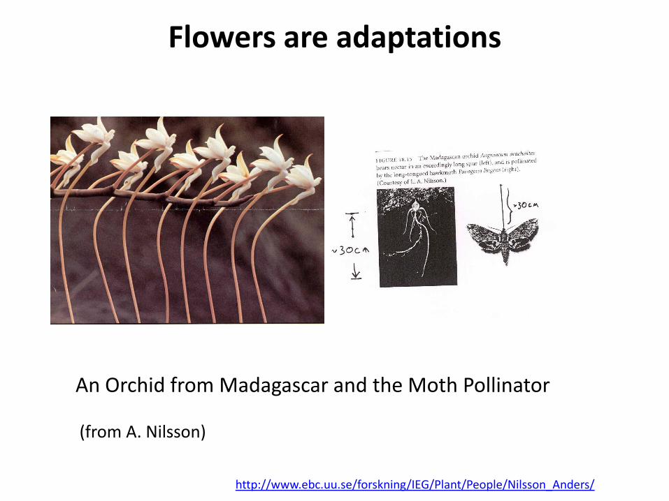
Flowers are adaptations

An Orchid from Madagascar and the Moth Pollinator (from A. Nilsson)

http://www.ebc.uu.se/forskning/IEG/Plant/People/Nilsson_Anders/

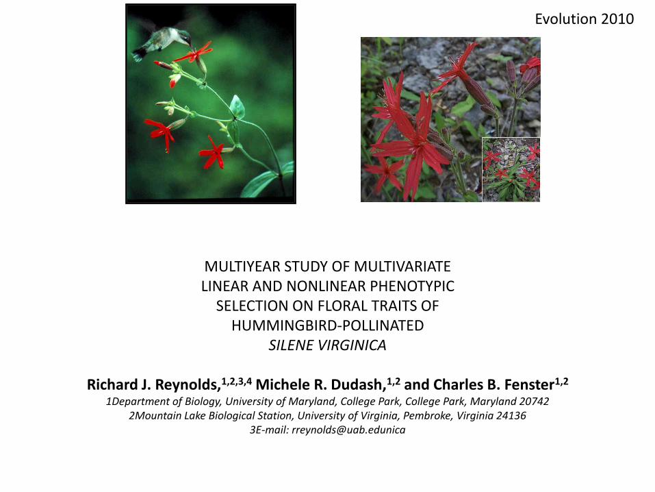
MULTIYEAR STUDY OF MULTIVARIATE LINEAR AND NONLINEAR PHENOTYPIC

SELECTION ON FLORAL TRAITS OF HUMMINGBIRD-POLLINATED

SILENE VIRGINICA

Richard J. Reynolds,1,2,3,4 Michele R. Dudash,1,2 and Charles B. Fenster1,2 1Department of Biology, University of Maryland, College Park, College Park, Maryland 20742

2Mountain Lake Biological Station, University of Virginia, Pembroke, Virginia 24136 3E-mail: rreynolds@uab.edunica

Evolution 2010

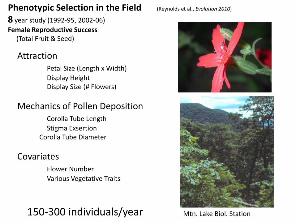
Attraction Petal Size (Length x Width)

Display Height Display Size (# Flowers)

Mechanics of Pollen Deposition Corolla Tube Length

Stigma Exsertion Corolla Tube Diameter

Covariates Flower Number

Various Vegetative Traits

Phenotypic Selection in the Field (Reynolds et al., Evolution 2010)

8 year study (1992-95, 2002-06)

Female Reproductive Success (Total Fruit & Seed)

150-300 individuals/year Mtn. Lake Biol. Station

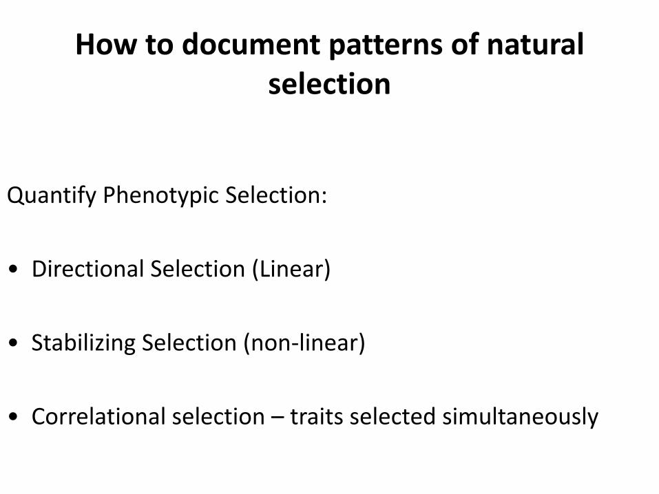
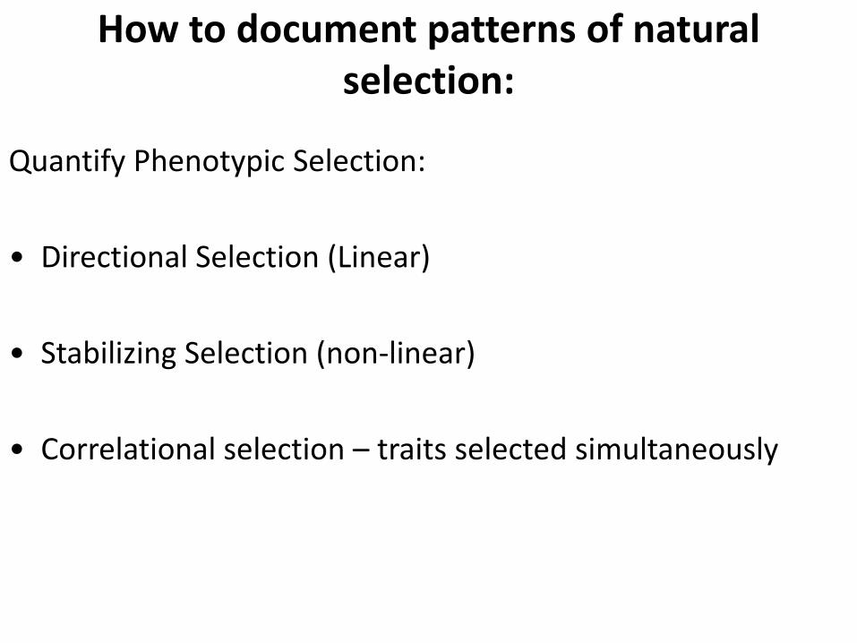
How to document patterns of natural selection

Quantify Phenotypic Selection:

• Directional Selection (Linear)

• Stabilizing Selection (non-linear)

• Correlational selection – traits selected simultaneously

-0.3

-0.2

-0.1

0

0.1

0.2

0.3

1992

1993

1994

1995

2003

2004

2005

2006

Life

time

Coh

ort 2

002

Life

time

Coh

ort 2

004

TL

PL

PW

TD

SE

DHT

sig

sig

sigsig

sig

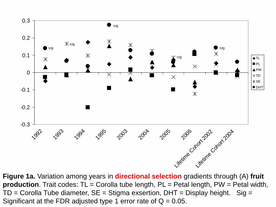
Figure 1a. Variation among years in directional selection gradients through (A) fruit

production. Trait codes: TL = Corolla tube length, PL = Petal length, PW = Petal width,

TD = Corolla Tube diameter, SE = Stigma exsertion, DHT = Display height. Sig =

Significant at the FDR adjusted type 1 error rate of Q = 0.05.

How to document patterns of natural selection:

Quantify Phenotypic Selection:

• Directional Selection (Linear)

• Stabilizing Selection (non-linear)

• Correlational selection – traits selected simultaneously

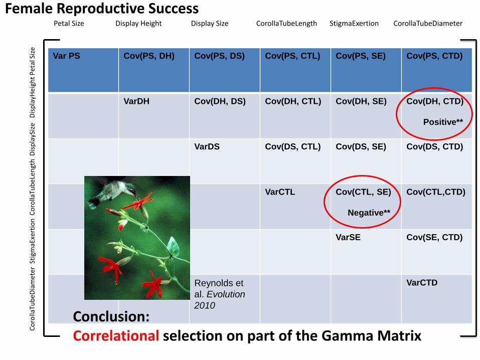
Petal Size Display Height Display Size CorollaTubeLength StigmaExertion CorollaTubeDiameter

C

oro

llaTu

beD

iam

eter

Sti

gmaE

xert

ion

Co

rolla

Tub

eLen

gth

Dis

pla

ySiz

e

Dis

pla

yHei

ght

Pet

al S

ize

Var PS Cov(PS, DH) Cov(PS, DS) Cov(PS, CTL) Cov(PS, SE) Cov(PS, CTD)

VarDH Cov(DH, DS) Cov(DH, CTL) Cov(DH, SE) Cov(DH, CTD)

Positive**

VarDS Cov(DS, CTL) Cov(DS, SE) Cov(DS, CTD)

VarCTL Cov(CTL, SE)

Negative**

Cov(CTL,CTD)

VarSE Cov(SE, CTD)

Reynolds et

al. Evolution

2010

VarCTD

Conclusion: Correlational selection on part of the Gamma Matrix

Female Reproductive Success

• Gene Flow – unifying or diversifying force, Fst

• Genetic Drift – random changes in allele frequencies within a population, effects >er for small than large populations

• Natural Selection – individual variation in survival and reproduction within a population

• Types of Natural Selection: Directional, Stabilizing, and Correlational

• Evolution – changes in allele frequencies owing to natural selection.

Highlights