Embed Size (px)
Citation preview
GENE EXPRESSION DATAANALYSIS
ZHANG ZONGHONG
NATIONAL UNIVERSITY OF SINGAPORE
2004
GENE EXPRESSION DATAANALYSIS
ZHANG ZONGHONG
(MB, Xi’an Jiao Tong Uni., PRC)
(Bachelor of Comp., Deakin Uni., Australia)
A THESIS SUBMITTED
FOR THE DEGREE OF MASTER OF SCIENCE
DEPARTMENT OF COMPUTER SCIENCE
NATIONAL UNIVERSITY OF SINGAPORE
2004
Name: ZHANG ZONGHONGDegree: Master of ScienceDept: Computer ScienceThesis Title: GENE EXPRESSION DATA ANALYSIS
Abstract
Data mining is the process of analyzing data in a supervised or unsupervised man-
ner to discover useful and interesting information that is hidden within the data.
Research in genomics is aimed at understanding the biological systems, by analyz-
ing their structure as well as their functional behaviour.
This thesis explore two area, unsupervised mining and supervised mining with
applications in Bioinformatics.
In the first part of this thesis, we generalize biclustering algorithm for microarray
gene expression data. We also improve the implementation of this framework and
design a novel algorithm called DBF (Deterministic Biclustering with Frequent
pattern mining).
In the second part of this thesis, we propose a simple yet very effective method
for gene selection for classification. The method can find minimal and optimal
subset of genes which can accurately classify gene expression data.

Acknowledgement
I would like to express my sincere thanks deep from my heart to the following who
give me great help for this thesis.
My supervisor, A/P Tan Kian Lee, helps me to conquer the difficulties in my
research and obtain the knowledge of Bioinformatics. His encouragement and con-
tinuous guidance is the source of my inspiration.
My Co-supervisor, Prof. Ooi Beng Chin, gives me the chance to study and the
most important, gives me convenient environment and support to do the research.
My collaborator in NUS, Mr Teo Meng Wee, Alvin whose discussions inspire
many constructive ideas.
My collaborator in NTU, Mr Chu Feng, et al. helps me on classification.
My friends, Miss Cao Xia, Miss Yang Xia and Mr Li Shuai Cheng, Mr Cui
Bing, Mr Cong Gao, Mr Li Han Yu, Mr Wang Wen Qiang, Mr. Zhou Xuan and all
the other members in EC database lab, whose friendship provides me a wonderful
atmosphere that makes my research work quite enjoyable.
My family, their unconditional support and love give me the confidence to
overcome all the struggles in my studies, and more important, in life.
My son, Samuel, where all my motivation and energy come from.
i

Contents
Acknowledgements i
1 Introduction 1
1.1 Background . . . . . . . . . . . . . . . . . . . . . . . . . . . . . . . 1
1.2 Motivation . . . . . . . . . . . . . . . . . . . . . . . . . . . . . . . . 2
1.3 Contributions of the Research . . . . . . . . . . . . . . . . . . . . . 3
1.4 Thesis Structure . . . . . . . . . . . . . . . . . . . . . . . . . . . . . 4
2 Gene Expression and DNA Microarray 5
2.1 Basics of Molecular Biology . . . . . . . . . . . . . . . . . . . . . . 5
2.1.1 DNA . . . . . . . . . . . . . . . . . . . . . . . . . . . . . . . 6
2.1.2 Genome, Chromosome, and Gene . . . . . . . . . . . . . . . 7
2.1.3 Gene Expression . . . . . . . . . . . . . . . . . . . . . . . . 8
2.2 Microarray Technique . . . . . . . . . . . . . . . . . . . . . . . . . . 9
2.2.1 Robotically Spotted Microarays . . . . . . . . . . . . . . . . 11
2.2.2 Oligonucleotide Microarrays . . . . . . . . . . . . . . . . . . 13
3 Related Works 15
3.1 Biclustering . . . . . . . . . . . . . . . . . . . . . . . . . . . . . . . 15
3.1.1 Cheng’s Algorithm on Biclustering . . . . . . . . . . . . . . 16
3.1.2 FLOC . . . . . . . . . . . . . . . . . . . . . . . . . . . . . . 18
ii
CONTENTS iii
3.1.3 δ-pCluster . . . . . . . . . . . . . . . . . . . . . . . . . . . . 22
3.1.4 Others . . . . . . . . . . . . . . . . . . . . . . . . . . . . . . 23
3.2 Classification . . . . . . . . . . . . . . . . . . . . . . . . . . . . . . 23
3.2.1 Single-slide Approach . . . . . . . . . . . . . . . . . . . . . . 24
3.2.2 Multi-Slide Methods . . . . . . . . . . . . . . . . . . . . . . 25
3.2.3 Nearest Shrunken Centroids: Recent Research Work on Gene
Selection . . . . . . . . . . . . . . . . . . . . . . . . . . . . . 28
3.3 Frequent Pattern Mining . . . . . . . . . . . . . . . . . . . . . . . . 29
3.3.1 CHARM . . . . . . . . . . . . . . . . . . . . . . . . . . . . . 30
3.3.2 Missing Data Estimation for Gene Microarray Expression Data 32
3.3.3 SVM . . . . . . . . . . . . . . . . . . . . . . . . . . . . . . . 32
4 Biclustering of Gene Expression Data 35
4.1 Formal Definition of Biclustering . . . . . . . . . . . . . . . . . . . 35
4.2 Framework of Biclustering . . . . . . . . . . . . . . . . . . . . . . . 37
4.3 Deterministic Biclustering with Frequent Pattern Mining (DBF) . . 38
4.4 Good seeds of possible biclusters from CHARM . . . . . . . . . . . 38
4.4.1 Data Set Conversion . . . . . . . . . . . . . . . . . . . . . . 39
4.4.2 Frequent Pattern Mining . . . . . . . . . . . . . . . . . . . . 41
4.4.3 Extracting seeds of biclusters . . . . . . . . . . . . . . . . . 42
4.5 Phase 2: Node addition . . . . . . . . . . . . . . . . . . . . . . . . . 44
4.6 Adding Deletion in Phase 2 . . . . . . . . . . . . . . . . . . . . . . 49
4.7 Experimental Study . . . . . . . . . . . . . . . . . . . . . . . . . . . 51
4.7.1 Experiment 1 . . . . . . . . . . . . . . . . . . . . . . . . . . 51
4.7.2 Experiment 2 . . . . . . . . . . . . . . . . . . . . . . . . . . 57
4.7.3 Experiment 3 . . . . . . . . . . . . . . . . . . . . . . . . . . 59

CONTENTS iv
5 Gene Selection for classification 61
5.1 Method of Gene Selection . . . . . . . . . . . . . . . . . . . . . . . 62
5.2 Experiment . . . . . . . . . . . . . . . . . . . . . . . . . . . . . . . 63
5.2.1 Experiment Result on Liver Cancer Data Set . . . . . . . . . 65
5.2.2 Experiment Result on Lymphoma Data Set . . . . . . . . . 65
5.2.3 Experiment Result on SRBCT Data Set . . . . . . . . . . . 66
6 Conclusion and Future Works 70
6.1 Conclusion . . . . . . . . . . . . . . . . . . . . . . . . . . . . . . . . 70
6.2 Future Work . . . . . . . . . . . . . . . . . . . . . . . . . . . . . . . 71
BIBLIOGRAPHY 73
Chapter 1
Introduction
Data mining is the process of analyzing data in a supervised or unsupervised man-
ner to discover useful and interesting information that is hidden within the data.
Many data mining approaches have been applied to genomics to aim at understand-
ing the biological systems, by analyzing their structures as well as their functional
behaviors.
1.1 Background
Recently developed DNA microarray technology has made it now possible for bi-
ologists to monitor simultaneously the expression levels of thousands of genes in a
single experiment. Microarray experiments include experiments during important
biological processes, such as cellular replication and the response to changes in the
environment, and across collections of related samples, such as tumor samples from
patients/tissues and normal persons/tissues.
Experiments of DNA microarray technology generate enormous amount of data
at a rapid rate. Analyzing such functional data combined with the structure infor-
mation would not be possible without effective and efficient computational tech-
1
CHAPTER 1. INTRODUCTION 2
niques. Microarray experiments give rise to numerous statistical questions, in di-
verse field such as image processing, experimental design, and discriminant analysis
[Aas01].
Elucidating patterns hidden in gene expression data to completely understand
functional genomics have grasped bioinformatics scientists’ tremendous attention.
However it is a huge challenge to comprehend and interpret the resulting mass of
data of microarray because of the large number of genes and complexity of biological
networks. Data mining techniques are essential techniques for genomic researchers
to explore natural structure and gain insights into the functional behaviors of genes
as well as to correlate structural information with functional information.
Data mining techniques can be divided into two categories, unsupervised tech-
niques and supervised techniques. Clustering is one of major processes in unsu-
pervised techniques, and Classification and prediction is one of major processes in
supervised techniques.
1.2 Motivation
In microarray data analysis, cluster analysis has been used to group genes with
similar function [Aas01]. Biclustering is a two-way clustering.
A bicluster of a gene expression data set captures the coherence of a subset
of genes and a subset of conditions. Biclustering algorithms are used to discover
biclusters whose subset of genes are co-regulated under the subset of conditions. Ef-
ficient and effective biclustering algorithm will overcome some problems associated
with previous work in this area.
On the other hand, in discriminant analysis (supervised learning), one builds a
classifier capable of discriminating between members and non-members of a given
class, and use the classifier to predict the class of genes of unknown function [Aas01].
CHAPTER 1. INTRODUCTION 3
Finding out the minimum gene combinations that can ensure highly accurate clas-
sification of disease by using supervised learning can reduce the computational
burden and noise of irrelevant genes. It also can simplify gene expression tests
while calling for further investigation into possible biological relationship between
these small amount of genes and disease development and treatment.
1.3 Contributions of the Research
First, we generalize a framework for biclusering and also present a novel approach,
called DBF (Deterministic Biclustering with Frequent pattern mining) to imple-
ment this framework in order to find biclusters in a more effective and efficient way.
Our general framework scheme comprises two phases, seeds generation and seeds
refinement. To implement this framework, in the first phase, we generate a set of
good quality biclusters based on frequent pattern mining. Such an approach not
only allows us to tap into the rich field of frequent pattern mining algorithms to
provide efficient algorithms for biclustering, but also provides a deterministic solu-
tion. In the second phase, the biclusters are further iteratively refined (enlarged) by
adding more genes and/or conditions. We evaluated our scheme against FLOC on
Yeast expression data set [CC00] which is based on Tavazoie et al. [THC+99] and
Human expression data [CC00] which is based on Alizadeh et al [AED+00]. Our
results show that the proposed scheme can generate larger and better biclusters.
Second, we propose a simple yet very effective method to select an optimal
subset of genes for classification. The method comprises two steps. In the first
phase, important genes are chosen using a ranking scheme, such as t-test [DP97]
[TTC98]. In the second phase, we test the classification capability of all simple
combinations of those genes found in the first phase by using a good classifier, a
support vector machine (SVM). The accuracy of our proposed method for Lym-

CHAPTER 1. INTRODUCTION 4
phoma data set [AED+00], and the liver data set [CCS+02] reaches 100% with 2
genes. Our approach perfectly classified the 4 sub-types of cancers with 3 genes
for data set of small round blue cell tumors (SRBCTs) of childhood [KWR+01]. It
is obvious that the method we proposed significantly reduces the number of genes
required for highly reliable diagnosis.
1.4 Thesis Structure
This thesis is organized into 6 chapters. A brief introduction of problems of mining
DNA microarray expression is presented in Chapter 1. Chapter 2 describes the con-
cept and procedures of biological technique, DNA microarray. Chapter 3 introduces
related works and theory in gene expression data analysis. Chapter 4 generalizes
a framework for biclustering, and presents our algorithm, DBF (Deterministic Bi-
clustering with Frequent pattern mining)in details as well as its experiment results.
This is followed by Chapter 5 which introduces our approach on gene selection for
classification (supervised learning) and its experiment results. Chapter 6 presents
the conclusion and outlines some areas for future work.
Chapter 2
Gene Expression and DNA
Microarray
2.1 Basics of Molecular Biology
It is well known that all living cells perform two types of functions: (1) Carrying
out various chemical reactions to maintain life which is performed by protein; (2)
Passing life information to the next generation. DNA is responsible for this function
since it stores and passes life information. And RNA is the intermediate between
DNA and proteins. RNA has some functions of proteins, as well as some of DNA’s.
All living cells contain chromosomes, large pieces of DNA containing hundreds
or thousands of genes, each of which specifies the composition and structure of a
single protein [Aas01]. Proteins are responsible for cellular structure, producing
energy and for reproducing human chromosomes. Differences in the abundance,
state and distribution of cell proteins lead to very distinct properties of an organism.
DNA provides information that is needed to code for proteins. Messenger RNA
(mRNA) is synthesized from a DNA template resulting in the transfer of generic
information from the DNA molecule to the mRNA. The mRNA is then translated
5
CHAPTER 2. GENE EXPRESSION AND DNA MICROARRAY 6
into protein.
2.1.1 DNA
DNA stores the instruction needed by the cell to perform daily life function. DNA
is a double stranded. Two strands line up antiparallel to each other. The double
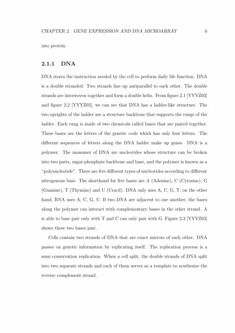
strands are interwoven together and form a double helix. From figure 2.1 [YYYZ03]
and figure 2.2 [YYYZ03], we can see that DNA has a ladder-like structure. The
two uprights of the ladder are a structure backbone that supports the rungs of the
ladder. Each rung is made of two chemicals called bases that are paired together.
These bases are the letters of the genetic code which has only four letters. The
different sequences of letters along the DNA ladder make up genes. DNA is a
polymer. The monomer of DNA are nucleotides whose structure can be broken
into two parts, sugar-phosphate backbone and base, and the polymer is known as a
“polynucleotide”. There are five different types of nucleotides according to different
nitrogenous base. The shorthand for five bases are A (Adenine), C (Cytosine), G
(Guanine), T (Thymine) and U (Uracil). DNA only uses A, C, G, T, on the other
hand, RNA uses A, C, G, U. If two DNA are adjacent to one another, the bases
along the polymer can interact with complementary bases in the other strand. A
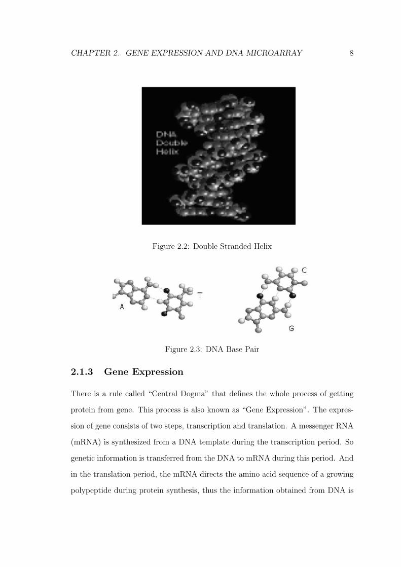
is able to base pair only with T and C can only pair with G. Figure 2.3 [YYYZ03]
shows these two bases pair.
Cells contain two strands of DNA that are exact mirrors of each other. DNA
passes on genetic information by replicating itself. The replication process is a
semi conservation replication. When a cell split, the double strands of DNA split
into two separate strands and each of them serves as a template to synthesize the
reverse complement strand.
CHAPTER 2. GENE EXPRESSION AND DNA MICROARRAY 7
Figure 2.1: Double Stranded DNA
2.1.2 Genome, Chromosome, and Gene
The genome is a complete set of DNA of an organism. And chromosomes are
strands of DNA wound around histone proteins. Humans have 22 pairs of chromo-
somes numbered 1 to 22 called autosomes and the X and Y sex chromosomes.
Each chromosome contains many genes, the basic physical and functional units
of heredity. Genes are specific sequences of bases that encode a protein or an
RNA molecule. Genes comprise of two of noncoding regions, whose functions may
include providing chromosomal structure integrity and regulating where, when and
in what quantity proteins are made [YYYZ03].
CHAPTER 2. GENE EXPRESSION AND DNA MICROARRAY 8
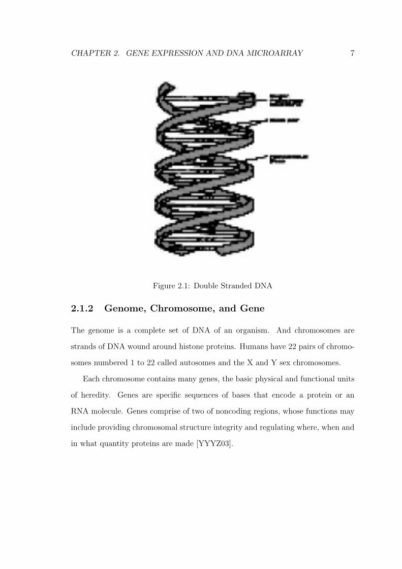
Figure 2.2: Double Stranded Helix
Figure 2.3: DNA Base Pair
2.1.3 Gene Expression
There is a rule called “Central Dogma” that defines the whole process of getting
protein from gene. This process is also known as “Gene Expression”. The expres-
sion of gene consists of two steps, transcription and translation. A messenger RNA
(mRNA) is synthesized from a DNA template during the transcription period. So
genetic information is transferred from the DNA to mRNA during this period. And
in the translation period, the mRNA directs the amino acid sequence of a growing
polypeptide during protein synthesis, thus the information obtained from DNA is
CHAPTER 2. GENE EXPRESSION AND DNA MICROARRAY 9
transferred to the protein.
In the whole process, the information flow that occurs during new protein syn-
thesis can be summarized as:
DNA → mRNA → Proteins
That is, the production of a protein begins with the information in DNA. That in-
formation is copied, or transcribed, in the form of mRNAs. The message contained
in the mRNAs is then translated into a protein. This process does not continue at
steady rate but only occurs when the protein is “needed”.
2.2 Microarray Technique
As mentioned before, the process of transcribing the gene’s DNA sequence into
mRNA that serves as a template for protein production is known as gene expression
[Aas01]. Gene expression describes how active a particular gene is. It is quantified
by the amount of mRNA from that gene.
The last ten years has seen the emergence of DNA microarray which enable
the gene expression analysis of thousands of genes simultaneously. DNA microar-
ray is fabricated by high-speed robotics, generally on glass but sometimes on nylon
substrates, for which probes with known identity are used to determine complemen-
tary binding, thus allowing massively parallel gene expression and gene discovery
studies.
The recent development of DNA microarray (1990) makes it possible to quickly,
efficiently and accurately measure the relative representation of each mRNA species
in the total cellular mRNA population [Aas01]. It is also known as RNA detection
microarrays, DNA chips, biochips or simply chips. There are usually five steps in
this technology [KKB03]:
1. Probe: this is the biochemical agent that finds or complements a specific
CHAPTER 2. GENE EXPRESSION AND DNA MICROARRAY 10
sequence of DNA, RNA, or protein from a test sample.
2. Arrays: the method for placing the probes on a medium or platform. Cur-
rent techniques include robotic spotting, electric guidance, photolithography,
piezoelectricity, fiber optics and microbeads. This step also specifies the type
of medium involved, such as glass slides, nylon meshes, silicon, nitrocellulose,
membranes, gels and beads.
3. Sample probe: the mechanism for preparing RNA from test samples. Total
RNA may be used, or mRNA may be selected using a polydeoxythymidine
(poly-dT) to bind the polyadenine (poly-A) tail. Alternatively, mRNA may
be copied into cDNA, using labeled nucleotides or biotinylated nucleotides.
4. Assay: How is the signal of expression being transduced into something more
easily measurable? Microarrays transduce gene expression into hybridization.
5. Readout: Microarrays techniques measure transduced signals and represent
the signals by measuring hybridization either using one or two dyes, or ra-
dioactive labels.
For the microarrays in common use, one typically starts by taking a specific bio-
logical tissue or system of interest, extracting its mRNA, and making a fluorescence-
tagged cDNA copy of this mRNA [KKB03]. cDNA is complementary DNA that
is synthesized from a mRNA template. This tagged cDNA copy called sample
probe is then hybridized to a slide containing a grid or array of single-stranded
cDNAs called probes which have been built or placed in specific locations on this
grid[KKB03]. A sample probe will only hybridize with its complementary probe.
Fluorescent is added either by using fluorescence-nucleotide bases when making the
cDNA copy of the RNA or by first incorporating biotinylated nucleotides, followed
CHAPTER 2. GENE EXPRESSION AND DNA MICROARRAY 11
by an application of fluorescence-labelled streptavidin which will bind to the bi-
otin. After several hours of the probe-sample probe hybridization process, a digital
scanner will record the brightness level at each grid location on the microarray that
correspond to particular RNA species. The brightness level is correlated with the
absolute amount of RNA in the original sample and by extension, the expression
level of the gene associated with this RNA.
There are two types of microarray techniques in common use: robotically
spotted and oligonucleotide microarrays.
2.2.1 Robotically Spotted Microarays
These kind of microarrays are shown in figure 2.4 [Aas01], are also known as cDNA
microarrays were first introduced at Stanford University and first described by
Mark Schema et. al in 1995.
DNA microarray, is fabricated by high-speed robotics, generally on glass but
sometimes on nylon substrates, for which probes with known identity are used to
determine complementary binding, thus allowing massively parallel gene expression
and gene discovery studies.
• Probe: cDNA sequences (length 0.6 - 2.4 kb) are spotted by robotic
• Target: in ”two-channel” design, sample solution (test) whose mRNA levels
are to be measured is labelled with fluorescence, e.g. Cye5 (red color), and a
control solution (reference) labelled with fluorescence Cye3 (green color)
• Hybridization: target sequence (mRNA) hybridizes with probe sequence (cDNA),
the amount of target sequences are measured by two light intensities (two col-
ors).
.
CHAPTER 2. GENE EXPRESSION AND DNA MICROARRAY 12
Figure 2.4: Robotically Spotted Microarrays
CHAPTER 2. GENE EXPRESSION AND DNA MICROARRAY 13
The result is a matrix, with each row representing a gene, each column a sam-
ple and each cell the expression ratio of the appropriate gene in the appropriate
sample. This ratio is the log(green/red) intensities of mRNA hybridizing at each
site measured.
2.2.2 Oligonucleotide Microarrays
The second popular class of microarrays in use has been most notably developed
and marketed by Affymetrix. Currently, over 1.5×10⁵ oligonucleotides of length 25
base pairs each, called 25-mers, can be placed on an array. These oligonucleotide
chips, or oligochips, are constructed using a photolithgraphic masking technique
[KKB03].
• Probe: oligonucleotide sequence (e.g. 25 bp, shorter than cDNA) fabricated
to surface in high density by chip-making technology
• Probe pair: one normal oligonucleotide sequence (perfect match, PM), another
similar oligo with one base changed (mismatch, MM). For each gene whose
expression in microarray has been designed to measure, there are between 16-
20 probe cells representing PM probes and a same number of cells representing
their associate MM probes. Collectively, these 32 to 40 probe cells are known
as a probe set [KKB03].
• Probe set: a collection of probe pairs for the purpose of detecting one mRNA
sequence.
• Target: again, fluorescently tagged. This time, the image is black-and-white:
no colors, figure 2.5 show a image of this microarray.
The result is a matrix, with each row representing a gene, each column a sample
and each cell the expression level of the appropriate gene in the appropriate sample.
CHAPTER 2. GENE EXPRESSION AND DNA MICROARRAY 14
Figure 2.5: Oligonucleotide Microarrays
This expression level is generated from derived or aggregate statistics for each probe
set.
Chapter 3
Related Works
3.1 Biclustering
Cluster analysis is currently a widely used technique for gene expression analysis.
It can be performed to identify genes that are regulated in a similar manner under
a number of experimental conditions [Aas01]. Biclustering is one of the clustering
techniques which have been applied to microarray data. Biclustering is two-way
clustering. A bicluster of a gene expression data set captures the coherence of
a subset of genes and a subset of conditions. Biclustering algorithms are used
to discover biclusters whose subset of genes are co-regulated under the subset of
conditions. This chapter reviews related works on this area.
Biclustering was introduced in the seventies [Har75], Cheng et al. [CC00] first
applied this concept to analyze microarray data and prove that biclustering is a
NP-hard problem.
There are a number of previous approaches for biclustering of microarray data,
including mean squared residue analysis, and the application of statistical bipartite
graph.
15

CHAPTER 3. RELATED WORKS 16
3.1.1 Cheng’s Algorithm on Biclustering
The algorithm proposed by Cheng and Church [CC00] begins with a large matrix
which is original data, and iteratively masks out null values and biclusters that
have been discovered. Each bicluster is obtained by a series of coarse and fine node
deletion, node addition, and the inclusion of inverted data.
In other words, Cheng’s work treats the whole original data set as a seed, then
they try to refine it through node deletion and node addition, after refining the
final bicluster will be masked with random data. Then in the following iteration,
it will treat the whole data set as another seed and refine it again, so on.
Node Deletion
The correctness and efficiency of node deletion algorithms in Cheng-2 are based on
a number of lemmas and theorem, i.e. lemma 1, lemma 2 and theorem 1 in which
rows (or columns) are treated as points in a space where a distance is defined
[CC00].
Lemma 1 Let S be a finite set of points in a space in which a non-negative real-
valued function of two arguments, d is defined. Let m(S) be a point that summarizes
the function
f(s) =∑x∈S
d(x, s).
Define the measure
E(S) =1
S
∑x∈S
d(x,m(S)).
Then, the removal of any non-empty subset
R ⊂ {x ∈ S : d(x,m(S)) > E(S)}

CHAPTER 3. RELATED WORKS 17
will make
E(S −R) < E(S).
Lemma 2 Suppose the set removal from S is
R ⊂ {x ∈ S : d(x,m(S)) > αE(S)}
with α ≥ 1. Then the reduction rate of the score E(S) can be characterized as
E(S)− E(S −R)
E(S)>
α− 1
|S|/|R| − 1
Theorem 1 The set of rows that can be completely or partially removed with the
net effect of decreasing the score of a bilcuster AIJ is
R = {i ∈ I;1
J
∑j∈J
(aij − aiJ − aIj + aIJ)2 > H(I, J)}
All these lemma and theorem are proved by in [CC00]. Cheng et. al. propose two
algorithms on node deletion, one is ”Single Node Deletion” 3.1 and ”Multiple Node
Deletion” 3.2. Cheng et al. suggest that to use the algorithm 3.2 before the matrix
is reduced to a manageable size, when ”Single Node Deletion” is appropriate.
Node Deletion
Cheng et. al. believes that the resulting δ-bicluster may not be maximal, which
means that some rows and columns may be added without increasing the score.
Lemma 3 [CC00] and theorem 2[CC00] provide a guideline for node addition.
Lemma 3 Let S, d, m(S), and E(S) be defined as same as those in Lemma 1.
Then, the addition to S of any non-empty subset
R ⊂ {x /∈ S : d(x,m(S)) ≤ E(S)}
will not increase the score E:
E(S + R) ≤ E(S).

CHAPTER 3. RELATED WORKS 18
Algorithm 3.1 Cheng(Single Node Deletion)
Input: A, a matrix of real numbers, δ ≥ 0, the maximum acceptable meansquared residue score.
Output: AIJ , a δ-bicluster that a sub-matrix of A with row set I and columnset J , with a score no larger than δ.
Initialization: I and J are initialized to the gene and condition sets in thedata and AIJ = A.
Iteration:1. Compute aiJ for all i ∈ I, aIj for all j ∈ J , aIJ , and H(I, J). If
H(I, J) <= δ, return AIJ .2. Find the row i ∈ I with the largest
di =i
J
∑j∈J
(aij − aiJ − aIj + aIJ)2
and the column j ∈ J with the largest
dj =1
I
∑i∈I
(aij − aiJ − aIj + aIJ)2
remove the row or column whichever with the larger d value by updatingeither I or J .
Theorem 2 The set of rows that can be completely or partially added with the net
effect of decreasing the score of a bicluster AIJ is
R = {i /∈ I;1
J
∑j∈J
(aij − aiJ − aIj + aIJ)2 ≤ H(I, J)}
The detailed algorithm for node addition is shown in algorithm 3.3.
Step 5 in the iteration adds inverted rows into the bicluster. These rows form
”mirror image” of the rest of the rows in the bicluster and can be interpreted as
co-regulated but receiving teh opposite regulation [CC00].
3.1.2 FLOC
J. Yang et al. [YWWY03] proposed a probabilistic algorithm (FLOC) to address
the issue of random interference in Cheng and Church’s algorithm. The general

CHAPTER 3. RELATED WORKS 19
Algorithm 3.2 Cheng(Multiple Node Deletion)
Input: A, a matrix of real numbers, δ ≥ 0, the maximum acceptable meansquared residue score, and α > 1, a threshold for multiple node deletion.
Output: AIJ , a δ-bicluster that a sub-matrix of A with row set I and columnset J , with a score no larger than δ.
Initialization: I and J are initialized to the gene and condition sets in thedata and AIJ = A.
Iteration:1. Compute aiJ for all i ∈ I, aIj for all j ∈ J , aIJ , and H(I, J). If
H(I, J) <= δ, return AIJ .2. Remove the rows i ∈ I with
i
J
∑j∈J
(aij − aiJ − aIj + aIJ)2 > αH(I, J)
3. Recompute aIj, aIJ , and H(I, J).4. Recompute the columns j ∈ J with
1
I
∑i∈I
(aij − aiJ − aIj + aIJ)2 > αH(I, J).
5. If nothing has been removed in the iterate, switch to Algorithm 3.1

CHAPTER 3. RELATED WORKS 20
Algorithm 3.3 Cheng (Node Addition)
Input: A, a matrix of real numbers, I,J signifying a δ-bicluster.Output: I
′and J
′such that I ⊂ I
′with the property that H(I
′, J
′) ≤
H(I, J).Iteration:
1. Compute aiJ for all i ∈ I, aIj for all j ∈ J , aIJ , and H(I, J).2. Add the columns j /∈ J with
i
I
∑i∈I
(aij − aiJ − aIj + aIJ)2 ≤ H(I, J)
3. Recompute aiJ , aIJ , and H(I, J).4. Add the rows i /∈ I with
1
J
∑j∈J
(aij − aiJ − aIj + aIJ)2 ≤ H(I, J).
5. For each row i still not in I, add its inverse if
1
J
∑j∈J
(−aij + aiJ − aIj + aIJ)2 ≤ H(I, J).
6.If nothing is added in the iterate, return the final I and J as I′and J
′.
CHAPTER 3. RELATED WORKS 21
process of FLOC starts at choosing initial biclusters (called seeds) randomly from
the the original data matrix, then proceeds with iterations of series of gene and con-
dition moves (i.e., selections or de-selections) aiming at achieving the best potential
residue reduction.
In FLOC, K initial seeds are constructed randomly. A parameter ρ is introduced
t control the size of a bicluster. For each initial bicluster, a random switch is
employed to determine whether a row or column should be included. Each row and
column is included in the bicluster with probability ρ. Consequently, each initial
seed is expected to contain M × ρ rows and N × ρ columns. If the percentage of
specified value in an initial cluster falls below α threshold, then we keep generating
new clusters until the percentage of specified values of all columns and rows satisfy
the α threshold.
Then FLOC proceeds to an iterative process to improve the quality of the
biclusters continuously. During each iteration, each row and each column are ex-
amined to determine its best action towards reducing the overall mean squared
residue. These actions are then performed successively to improve the biclustering
[YWWY03].
During each iteration in the second phase, each row and each column are exam-
ined to determine its best action toward reducing the overall mean squared residue.
These actions are then performed successively to improve the biclustering. An ac-
tion is defined with respect to row (or column) and a bicluster. There are k actions
associated with each row (or column), one for each bicluster. For a given row (or
column) x and a bicluster c the action Action(x, c) is defined as the change of
membership of x with respect to c. If x is already included in c, then Action(x, c)
represents the removal x from the bicluster c. Otherwise, it denotes the addition
of x to the bicluster c [YWWY03].
CHAPTER 3. RELATED WORKS 22
The concept, gain is introduced by J. Yang et al. to assess the amount of
improvement that can be brought by an action. The detailed definition of gain in
chapter 4, see definition 1.
After the best action is identified for every row (or column), these N + M
actions are then performed sequentially. The best biclustering obtained during the
last iteration, denote by best−biclustering, is used as the initial biclustering of the
current iteration. Let Biclusteringi be the set of biclusters after applying the first
i actions. After applying all actions, M + N sets of biclusterings will be produced.
Among them, if any biclsutering with all r-biclusters has a large aggregated volume
than that of best − biclustering, then there is an improvement in the current
iteration. The biclsutering with the minimum average residue is stored in best −biclustering and the process continues to the next iteration. Otherwise, there is no
improvement in the current iteration and the process terminates. The biclustering
stored in best − biclustering is then returned as the final result [YWWY03]. At
iteration, the set of actions are performed according to a random weighted order
[YWWY03].
3.1.3 δ-pCluster
Another approach is the comparison of pattern similarity by H. Wang [WWYY02],
it focuses on pattern similarity of sub-matrices. This method clusters expression
data matrix row-wise as well as column-wise to find object-pair MDS (Maximum
Dimension Set) and column-pair MDS. After pruning off invalid MDS, a prefix tree
is formed and a post-order traversal of the prefix tree is performed to generate the
desired biclusters.
CHAPTER 3. RELATED WORKS 23
3.1.4 Others
Besides these data mining algorithms, G. Getz [GLD00] devised a coupled two-way
iterative clustering algorithm to identify biclusters. The notion of a plaid model
was introduced by L. Lazzeroni [LO02]. It describes the input matrix as a linear
function of variables corresponding to its biclusters and an iterative maximization
process of estimating a model is presented. A. Ben-Dor [BDCKY02] defined a
bicluster as a group of genes whose expression levels induce some linear order across
a subset of the conditions, i.e., an order preserving sub-matrix. They also proposed
a greedy heuristic search procedure to detect such biclusters. E. Segal [STG+01]
described many probabilistic models to find a collection of disjoint biclusters which
are generated in a supervised manner.
The idea of using bipartite graph to discover statistically significant bicluster
was proposed by A. Tanay [TSS02]. In this method, the authors proposed a bi-
partite graph G generated from expression data set. A subgraph of G essentially
corresponds to a bicluster. Weights are assigned to the edges and non-edges of the
graph, such that the weight of a subgraph will correspond to the edges’ statistical
significance. The basic idea is to find heavy subgraph in a bipartite graph as such
a subgraph is a statistically significant bicluster.
3.2 Classification
In order to identify informative genes, many approaches have been proposed, ac-
cording to [Aas01], there are two main group of approaches for identifying differen-
tially expressed genes. Single-slide methods refer to methods in which the decision
about gene differentially expressed in a sample is based on data from only this gene
and sample. Multiple-slide methods on the other hand, use the expression ratios
CHAPTER 3. RELATED WORKS 24
from several samples to decide whether a gene is differentially expressed.
3.2.1 Single-slide Approach
Early analysis of microarray data relied on cut-offs to identify differentially ex-
pressed genes. Such as Shena et. al. [SSH+96] declare a gene differentially ex-
pressed if the expression level differs more than a factor of 5 in the two mRNA
samples. De Risis et al. [DPB+96] identify differentially expressed gene using a ±3
cut-off for the log ratios of the fluorescence intensities, where the intensities first
are standardized with respect to the mean and standard deviation of the log ratios
for a set of genes which are believed not to be differentially expressed between the
two cell types of interest.
Other methods have focused on probabilistic modelling of the (R, G) pairs.
The method proposed by Chen et al. [CDB97] can be viewed as producing a set of
hypothesis tests, one for each gene on the microarray, in which the null hypothesis
for a gene is that the expectation of both intensity signals are equal, and the
alternative is that they are unequal. When an observed gene expression ratio R/G
falls in the tails of the null sampling distribution, the null hypothesis is rejected
and the gene is declared significantly expressed.
Sapir et al. [SC00] present an algorithm for estimating the posterior probability
of differential expression of genes from microarray data. Their method is base on
an orthogonal linear regression of the signals obtained from the two color channels.
Residuals from the regression are modelled as a mixture of a common component
and a differentially expressed component.
Newton et al. [NKR+01] consider a hierarchical model (Gamma-Gamma-Bernoulli
model) for (R, G) and suggest identifying differentially expressed genes based on
the posterior odds of change under this model.
CHAPTER 3. RELATED WORKS 25
3.2.2 Multi-Slide Methods
While the single-slide methods for identifying differential expression is base only on
the expression ratio of the gene in question, multi-slide methods use the expression
ratios from several samples to decide whether a gene is differentially expressed.
Such as different expression level of a certain gene in classes, healthy/sick, cancer
type1/cancer type2, normal/mutant, treatment/control and so on. Below is some
of the multi-slide methods.
T-Statistics
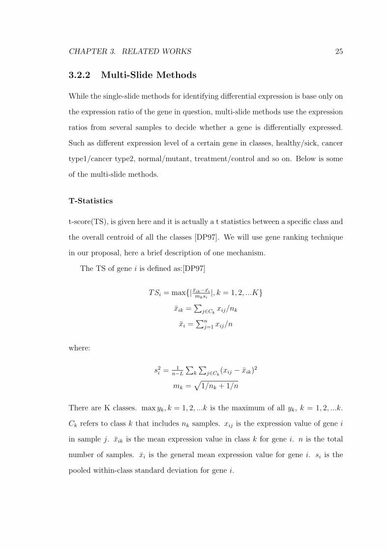
t-score(TS), is given here and it is actually a t statistics between a specific class and
the overall centroid of all the classes [DP97]. We will use gene ranking technique
in our proposal, here a brief description of one mechanism.
The TS of gene i is defined as:[DP97]
TSi = max{| xik−xi
mksi|, k = 1, 2, ...K}
xik =∑
j∈Ckxij/nk
xi =∑n
j=1 xij/n
where:
s2i = 1
n−L
∑k
∑j∈Ck
(xij − xik)2
mk =√
1/nk + 1/n
There are K classes. max yk, k = 1, 2, ...k is the maximum of all yk, k = 1, 2, ...k.
Ck refers to class k that includes nk samples. xij is the expression value of gene i
in sample j. xik is the mean expression value in class k for gene i. n is the total
number of samples. xi is the general mean expression value for gene i. si is the
pooled within-class standard deviation for gene i.
CHAPTER 3. RELATED WORKS 26
Analysis of Variance
Kerr et al. [KMC00] apply techniques from the analysis of variance (anova) to
determine differentially expressed genes. They assume a fixed effect linear model
for the intensities, with terms accounting for dye, slide, treatment, and gene main
effects, as well as a few interactions between these effects. Differentially expressed
genes are identified based on contrasts for the treatment × genes interactions
[Aas01].
Neighborhood
Golub et al. [GST+99] identify informative genes with neighborhood analysis in
their early work. Briefly, they define an idealized expression pattern, corresponding
to a gene that is uniformly high in one class and uniformly low in the other. Then
they identify the genes that are more correlated with this idealized expression
pattern than what would be expected by chance [Aas01].
Ratio of Between-Group to Within-Groups Sum of Squares
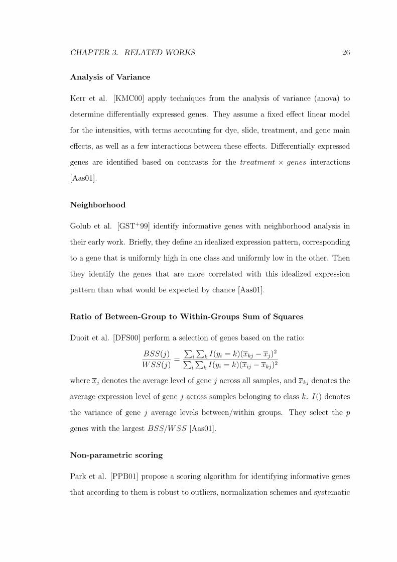
Duoit et al. [DFS00] perform a selection of genes based on the ratio:
BSS(j)
WSS(j)=
∑i
∑k I(yi = k)(xkj − xj)
2
∑i
∑k I(yi = k)(xij − xkj)2
where xj denotes the average level of gene j across all samples, and xkj denotes the
average expression level of gene j across samples belonging to class k. I() denotes
the variance of gene j average levels between/within groups. They select the p
genes with the largest BSS/WSS [Aas01].
Non-parametric scoring
Park et al. [PPB01] propose a scoring algorithm for identifying informative genes
that according to them is robust to outliers, normalization schemes and systematic
CHAPTER 3. RELATED WORKS 27
errors such as chip-to-chip variation. It starts with the gene expression matrix,
the expression levels for a gene is sorted from the smallest to the largest. Then,
the sorted expression levels are related to the class labels of the corresponding
samples, producing a sequence of 0’s and 1’s. How closely the 0’s and 1’s are
grouped together is a measure of the correspondence between the expression levels
and the group membership. If a particular gene can be used to divide the groups
exactly, one would observe a sequence of all 0’s followed by all 1’s, or vice versa.
The score of a gene is defined to be the smallest number of swaps of consecutive
digits necessary to arrive at a perfect splitting. With the above score, the genes
may be ordered according to their potential significance. To determine the number
of genes sufficient in categorizing the samples with known classes, one compares
the distributions that arise as the more significant genes are successively deleted
from the data, to a ”null distribution” obtained randomly permuting the columns
of the original expression matrix [Aas01].
Likelihood Selection
Keller et al. [KSHR00] use likelihood selection of genes for their naive Bayes
classifier. In the two class cases, they select two sets of genes, S1, S2 such that for
all genes in set S1:
L1 À 0andL2 > 0
and for all genes in set S2:
L1 > 0andL2 À 0
Here L1 and L2 are two relative log likelihood scores defined by:
L1 = logP (class1|trainingsamplesofclass1)−logP (class2|trainingsamplesofcalss1)
L2 = logP (class2|trainingsamplesofclass2)−logP (class1|trainingsamplesofcalss2)

CHAPTER 3. RELATED WORKS 28
The ideal gene for the naive Bayes classifier would be expected to have both L1 and
L2 much greater than zero, indicating that it on average votes for class 1 on training
samples of class 1, and for class 2 on training samples of class 2. In practice, it is
difficult to find genes for which both L1 and L2 much greater than zero. Hence, as
shown above, one of the likelihood scores is maximized while merely requiring the
other to be greater than zero [Aas01].
3.2.3 Nearest Shrunken Centroids: Recent Research Work
on Gene Selection
Tibshirani et al. [THNC03] propose a method called ”nearest shrunken centroid”
which uses de-noised version of the centroids as prototypes for each class.
Let xij be the expression for genes i = 1, 2, ...p and samples j = 1, 2, ...n. There
are 1, 2, ...K classes, and Ck be indices of the nk samples in class k. The ith com-
ponent of the centroid for class k is xik =∑
i∈Ckxij/nk, the mean expression value
in class k for gene i; the ith component of theoverall centroid is xi =∑n
j=1 xij/n.
They shrink the class centroids towards the overall centroids. However, they first
normalize by the within class-standard deviation for each gene. Let
dik =xik − xi
mksi
where si is the pooled within-class standard deviation for gene i:
s2i =
1
n−K
∑
k
∑i∈Ck
(xij − xik)2
and mk =√
1/nk + 1/n makes the denominator equal to the estimated standard
error of the numerator in dik. Thus dik is a t-statistic for gene i, comparing class k
to the average class. The equation is re-written as:
xik = xi + mksidik
CHAPTER 3. RELATED WORKS 29
their proposal shrinks each dik towards zero, giving d′ik and new shrunken cen-
troids or prototypes
x′ik = xi + mksid
′ik
The shrinkage they use is called soft − thresholding: each dik is reduced by an
amount∆ in absolute value, and is set to zero if its absolute value is less than zero.
Algebraically, this is expressed as
d′ik = sign(dik)(|dik| −∆)+
where + means positivepart (t+ = t if t > 0, and zero otherwise). Since many of the
xik will be noisy and close to the overall mean xi, soft-threshold produces ”better”
(more reliable) estimates of the true means. This method has a nice property
that many of the components (genes) are eliminated as far as class prediction is
concerned, if the shrinkage parameter ∆ is large enough. Specifically if for a gene
i, dik is shrunken to zero for all classes k, then the centroid for gene i is xi, the
same for all classes [THNC03].
3.3 Frequent Pattern Mining
Here we present one of the fundamental techniques in data mining, frequent pattern
mining, which is employed in our algorithm for biclustering.
Mining frequent patterns or itemsets is a fundamental and essential problem in
many data mining applications. These applications include the discovery of associ-
ation rules, strong rules, correlations, sequential rules, episodes, multi-dimensional
patterns, and many other important discover tasks [HK01]. The problem is defined
as: Given a large database of item transactions, find all frequent itemsets, where
a frequent itemset is one the occurs in at least a user-specified percentage of the
database [ZH02].
CHAPTER 3. RELATED WORKS 30
3.3.1 CHARM
CHARM was proposed by [ZH02], and has been shown to be an efficient algorithm
for closed itemset mining. Closed sets are lossless in the sense that they uniquely
determine the set of all frequent itemsets and their exact frequency. At the same
time closed sets can themselves be orders of magnitude smaller than all frequent
sets, especially on dense databases.
CHARM enumerates closed sets using a dual itemset-tidset search tree,i.e. it
simultaneously explores both the itemset space and transaction space, over a novel
IT−tree (itemset-tidset tree) search space. CHARM uses an efficient hybrid search
that skips many levels of the IT − tree to quickly identify the frequent closed item-
sets, instead of having to enumerate many possible subsets. It also uses a fast
hash-based approach to eliminate non-closed itemsets during subsumption check-
ing. CHARM utilizes a novel vertical data representation called diffsets technique
to reduce the memory footprint of intermediate computations. Diffsets keep track
of differences in the tids of a candidate pattern from its prefix pattern. Diffsets
drastically cut down (by order of magnitude) the size of memory required to store
intermediate results [ZH02]. CHARM is employed by our biclustering algorithm,
DBF.
The pseudo-code for CHARM [ZH02] is shown in algorithm 3.4.The algorithm
starts by initializing the prefix class [P ], of nodes to be examined, to the frequent
single items and their tidsets in Line 1. Charm assumes that the elements in
[P ] are ordered according to a suitable total order f . The main computation is
performed in CHARM-EXTEND which returns the set of closed frequent itemsets
C. CHARM-EXTEND is responsible for considering each combination of IT-pairs
appearing in the prefix class [P ] [ZH02].

CHAPTER 3. RELATED WORKS 31
Algorithm 3.4 CHARM
1. [P ] = {Xi × t(Xi) : Xi ∈ τ ∧ σ(Xi ≥ minsup}2: CHARM-EXTEND ([P ], C = φ)3: return C //all closed sets
CHARM-EXTEND ([P ], C = φ):4: for eachXi × t(Xi) in [P ]5: [Pi] = φ and X = Xi
6: for each Xj × t(Xj) in [P ], with Xj ≥f Xi
7: X = X ∪Xj and Y = t(Xi) ∩ t(Xj)8: CHARM-PROPERTY([P ], [Pi]9: if([Pi] 6= φ) then CHARM-EXTEND ([Pi], C)10: delete ([Pi])11: C = C ∪X //if X is not subsumed
CHARM-PROPERTY ([P ], [Pi]):12: if (σ(X) ≥ minisup)13: if t(Xi) = t(Xj) then //Property 114: Remove Xj from [P ]15: Replace all Xi with X16: else if t(Xi) ⊂ t(Xj) then //Property 217: Replace all Xi with X18: else if t(Xi) ⊃ t(Xj) then //Property 319: Remove Xj from [P ]20: Add X×Y to [Pi] //use ordering f21: else if t(Xi) 6= t(Xj) then //Property f22: Add X×Y to [Pi] //use ordering f
CHAPTER 3. RELATED WORKS 32
3.3.2 Missing Data Estimation for Gene Microarray Ex-
pression Data
Gene expression microarray experiment can generate data sets with multiple miss-
ing expression values [TCS+01]. Two data sets we use in our work includes such
missing data. There are only small number of missing data in yeast data we use,
we ignore these missing data and accept biclusters with a percentage of specified
value is equal or bigger than the percentage of specified value in the original data.
However, since there are a large number of missing data in the second data set,
lymphoma expression data, it is hard to find a bicluster with the required percent-
age of specified value. So we adopt a missing value estimation method for gene
expression microarray data set.
O. Troyanskaya et al. provide a comparative study of several methods for
the estimation of missing values in gene expression data [TCS+01]. They im-
plemented and evaluated three methods: a Singular Value Decomposition (SVD)
based mehtod (SVMimpute), weighted K-nearest neigbores (KNNimpute), and row
average.
3.3.3 SVM
There are a large number of classifiers in supervised learning area, such as Support
Vector Machine(SVM), Nearest Neighbour, Classification Tree, Voted Classifica-
tion, Weighted Gene Voting, Bayesian Classification, Fuzzy Neural Network, etc.
In the following, SVM is further described as we used it in our study.
Support vector machines (SVM) is a family of learning algorithms. The The-
ory behind SVM was developed by Vapnik and Chervonenkis in the sixties and
seventies. It has been successfully applied to all sorts of classification issues after
its first practical implementation in nineties. Recently SVM have been applied to

CHAPTER 3. RELATED WORKS 33
biological area, including gene expression data analysis and protein classification.
According to [Aas01], let y be the gene expression vector to be the gene expres-
sion vector to be classified. The SVM classifies y to either -1 or 1 using
c(y) =
1 if L(y) > 0
-1 if otherwise(3.1)
where the discriminant function is given by
L(y) =T∑
i=1
αiciK(y, yi), (3.2)
where {yi}Ti=1 is a set of training vectors and {ci}T
i=1 are the corresponding
classes (ci ∈ −1, 1). K(y, yi) is denoted a kernel and is often chosen as a polynom
of degree d, i.e.
K(y, yi) = (yT yi + 1)d (3.3)
Finally, αi is the weight of training sample yi. It represents the strength with
which that sample is embedded in the final decision function. Only a subset of
the training vectors will be associated with a non-zero αi. These vectors are called
support vectors.
The process of finding the weights αi that can maximize the distance of two
classes in the training samples is well known as training of SVM.
The aim of training process is to get a set of weights that maximize the objective
function:
J(α) =T∑
i=1
αi(2− ciL(yi)) (3.4)
subject to the following constraints

CHAPTER 3. RELATED WORKS 34
αi ≥ 0∑
i
αici = 0 i = 1, ..., T (3.5)
The output of learning result is the optimized set of weights α1, α2, ..., αT .
The above is a brief description of SVM for binary classification. Many re-
searchers have extended it for multi-classification. Several methods have been
proposed for multi-classification, such as ”one-against-all”, ”one-against-one” and
DAGSVM(Direct Acyclic Graph Support Vector Machines) etc.
According to study done by [CL02], the ”one-against-one” and DAG methods
are more suitable for practical use than the other methods.
Chapter 4
Biclustering of Gene Expression
Data
In this chapter we give detailed our proposal of biclustering on gene expression
data and experiment result.
4.1 Formal Definition of Biclustering
Let = = {A1, . . . , AM} be the set of genes, and < = {O1, . . . , ON} be the set of
conditions of a microarray expression expression data. The gene expression data
is represented as a M ×N matrix where each entry dij in the matrix corresponds
to the logarithmic of the relative abundance of the mRNA of a gene Ai under a
specific condition Oj. We note that dij can be a null value.
A bicluster captures the coherence of a subset of genes under a subset of condi-
tions. In [CC00], the degree of coherence is measured using the concept of the mean
squared residue, which represents the variance of a particular subset of genes under
a particular subset of conditions with respect to the coherence. The lower the mean
squared residue of a subset of genes under a subset of conditions, the more similar
35
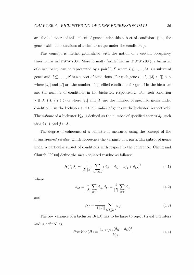
CHAPTER 4. BICLUSTERING OF GENE EXPRESSION DATA 36
are the behaviors of this subset of genes under this subset of conditions (i.e., the
genes exhibit fluctuations of a similar shape under the conditions).
This concept is further generalized with the notion of a certain occupancy
threshold α in [YWWY03]. More formally (as defined in [YWWY03]), a bicluster
of α occupancy can be represented by a pair(I, J) where I ⊆ 1, ..., M is a subset of
genes and J ⊆ 1, ..., N is a subset of conditions. For each gene i ∈ I, (|J ′i |/|J |) > α
where |J ′i | and |J | are the number of specified conditions for gene i in the bicluster
and the number of conditions in the bicluster, respectively. For each condition
j ∈ J , (|I ′j|/|I|) > α where |I ′j| and |I| are the number of specified genes under
condition j in the bicluster and the number of genes in the bicluster, respectively.
The volume of a bicluster VIJ is defined as the number of specified entries dij such
that i ∈ I and j ∈ J .
The degree of coherence of a bicluster is measured using the concept of the
mean squared residue, which represents the variance of a particular subset of genes
under a particular subset of conditions with respect to the coherence. Cheng and
Church [CC00] define the mean squared residue as follows:
H(I, J) =1
|I| |J |∑
i∈I,j∈J
(dij − diJ − dIj + dIJ)2 (4.1)
where
diJ =1
|J |∑j∈J
dij, dIj =1
|I|∑i∈I
dij (4.2)
and
dIJ =1
|I |J ||∑
i∈I,j∈J
dij (4.3)
The row variance of a bicluster B(I,J) has to be large to reject trivial biclusters
and is defined as
RowV ar(H) =
∑i∈I,j∈J(dij − diJ)2
VIJ
(4.4)
CHAPTER 4. BICLUSTERING OF GENE EXPRESSION DATA 37
where VIJ is the volume of H(I,J). A bicluster H(I,J) is a good bicluster if
H(I, J) < δ for some user-specified δ ≥ 0 and its RowVar(H) is larger than some
user-specified β > 0.
4.2 Framework of Biclustering
We find that the problem with Cheng’s is deterministic, but it suffers from random
interference. As pointed in [YWWY03], this interference caused by masking of null
values and discovered biclusters with random numbers. Although the random data
is unlikely to form any fictitious pattern, there exists a substantial risk that these
random numbers will interfere with the future discovery of biclusters, especially
those ones that have over-lap with the discovered ones [YWWY03].
On the other hand, FLOC is a probabilistic algorithm which can not guarantee
the quality of final biclusters. Our study shows that the quality of final biclusters
found by FLOC is very much dependent on the initial random seeds it choose.
However FLOC is efficient.
An intuition tells us that it will be better to have a algorithm which is deter-
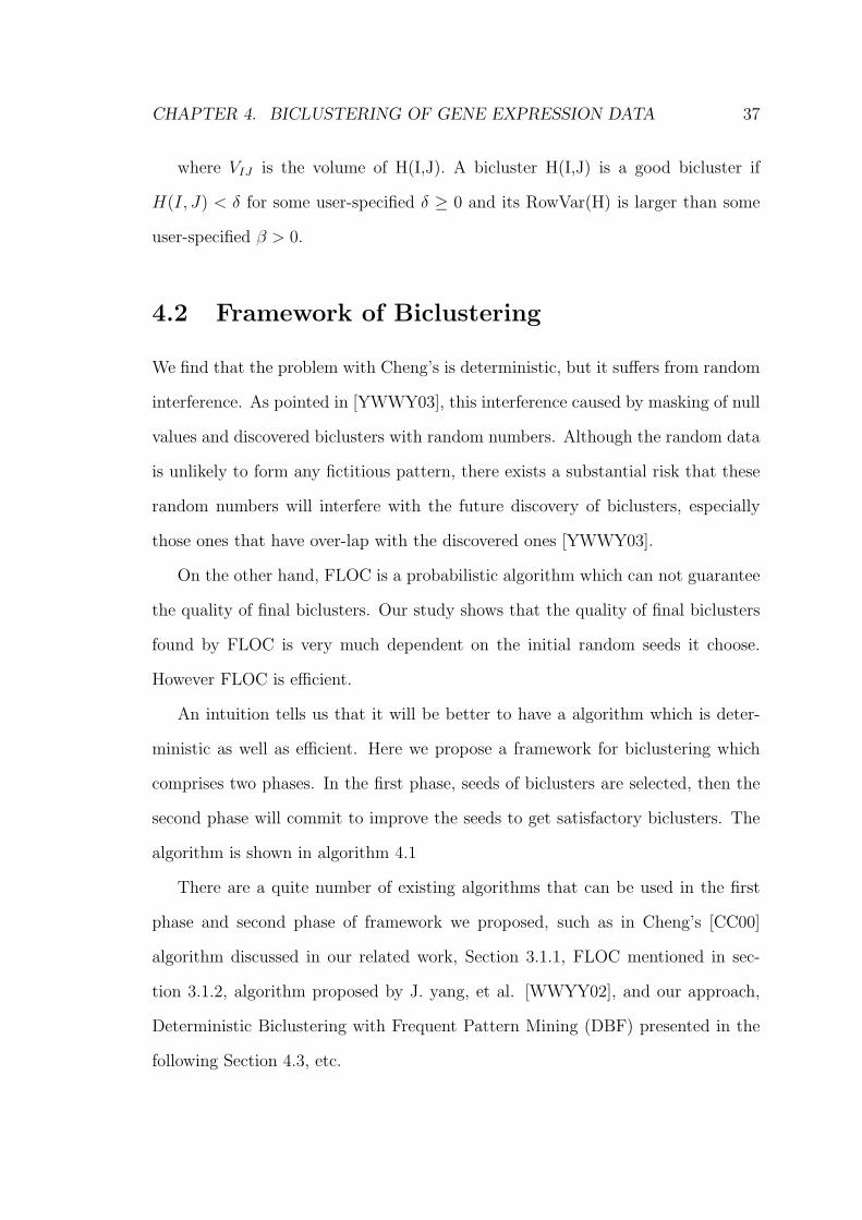
ministic as well as efficient. Here we propose a framework for biclustering which
comprises two phases. In the first phase, seeds of biclusters are selected, then the
second phase will commit to improve the seeds to get satisfactory biclusters. The
algorithm is shown in algorithm 4.1
There are a quite number of existing algorithms that can be used in the first
phase and second phase of framework we proposed, such as in Cheng’s [CC00]
algorithm discussed in our related work, Section 3.1.1, FLOC mentioned in sec-
tion 3.1.2, algorithm proposed by J. yang, et al. [WWYY02], and our approach,
Deterministic Biclustering with Frequent Pattern Mining (DBF) presented in the
following Section 4.3, etc.
CHAPTER 4. BICLUSTERING OF GENE EXPRESSION DATA 38
Algorithm 4.1 Framework of Biclustering
Input: Gene expression data matrixOutput: Qualified biclusters.Steps:
Phase One:Seeds Generation
Phase Two:Refine Seeds got in Phase One
Return Final Biclusters.
4.3 Deterministic Biclustering with Frequent Pat-
tern Mining (DBF)
In this section, I shall present our proposed, Deterministic Biclustering with Fre-
quent Pattern Mining (DBF) scheme to discover biclusters and its experiment re-
sults. Our scheme is actually an implementation of our proposed frame algorithm
for biclustering. Our scheme comprises two phases. Phase 1 generates a set of good
quality biclusters using a frequent pattern mining algorithm. While any frequent
pattern mining algorithm can be used, we have employed CHARM developed by
[ZH02] in our work. A more efficient algorithm will only improve the efficiency of
our approach. In phase 2, we try to enlarge the volume of the biclusters generated
in phase 1 to make them as maximal as possible while keeping the mean squared
residue low. We shall discuss the two phases below.
4.4 Good seeds of possible biclusters from CHARM
In general, a good seed of possible bicluster is actually a small bicluster whose mean
squared residue has reached the requirement but the volume is not maximal. A
small bicluster corresponds to a subset of genes which change or fluctuate similarly
under a subset of conditions. Thus, the problem of finding good seeds of possible

CHAPTER 4. BICLUSTERING OF GENE EXPRESSION DATA 39
biclusters could be transformed to mining similarly fluctuating patterns from a
microarray expression data set. Our approach comprises three steps. First, we
need to translate the original microarray expression data set to a pattern data set.
In this work, we treat the fluctuating pattern between two consecutive conditions
as an item, and each gene as a transaction. An itemset would then be a set of genes
that has similar changing tendency over sets of consecutive conditions. Second, we
need to mine the pattern set to get frequent patterns. Finally, we will post-process
the mining output to extract the good biclusters we need. This will also require us
to map back the itemsets into conditions.
4.4.1 Data Set Conversion
In order to capture the fluctuating patterns of each gene under conditions, we first
convert the original microarray data set to a big matrix whose rows represent genes,
columns represent edges of every two adjacent conditions. An edge of every two
conditions represents the directional change of a gene expression level under two
conditions. The conversion process involves the following steps.
1. Calculate angles of edge of every two conditions: Each gene in each row re-
mains unchanged. Each condition (column) is converted to an edge of ev-
ery two adjacent conditions. For a given matrix data set G × J Where
G = {g1, g2, g3, . . . , gm} is a set of genes and J = {a, b, c, d, e . . .} is a set of
conditions. After conversion, the new matrix should be G × JJ . Where
G = {g1, g2, g3, . . . , gm} is still the original set of genes, however, JJ =
{ab(arctan(b− a)), bc(arctan(c− b)), cd(arctan(d− c)), de(arctan(d− e)), . . .}is collection angles for edges of every two adjacent original conditions. In the
newly derived matrix, each column represents the angle of edges under every
two adjacent conditions. Table 4.1 shows a simple example of an original
CHAPTER 4. BICLUSTERING OF GENE EXPRESSION DATA 40
data set, table 4.2 shows the process of conversion and table 4.3 shows the
new matrix after conversion.
Table 4.1: Example of Original Matrix
Genes Conditionsa b c d e
g1 1 3 5 7 8g2 2 4 6 8 12g3 4 6 8 10 11
Table 4.2: Process of ConversionGenes Conditions
ab bc cd deg1 arctan(3-1) arctan(5-1) arctan(7-5) arctan(8-7)g2 arctan(4-2) arctan(6-4) arctan(8-6) arctan(12-8)g3 arctan(6-4) arctan(8-6) arctan(10-8) arctan(11-10)
Table 4.3: New Matrix after Conversion
Genes Conditionsab bc cd de
g1 63.43 75.96 80.54 45g2 63.43 75.96 80.54 75.96g3 63.43 75.96 80.54 45
2. Bin generation: It is obvious that the angle of each edge should be within
range, 0 degree to 180 degree. We know that two edges are similar if the angles
of two edges are equal. However these are perfect similar edges. Under our
situation, as long as angles of edges are within the same range predefined,
we will consider they are similar. Thus, at this step, we divide 0-180 into
different bins. Each bin is set to the same or different size. For example, if
there are 3 bins, the first bin contains edges with angle of 0 to 5 and 175 to
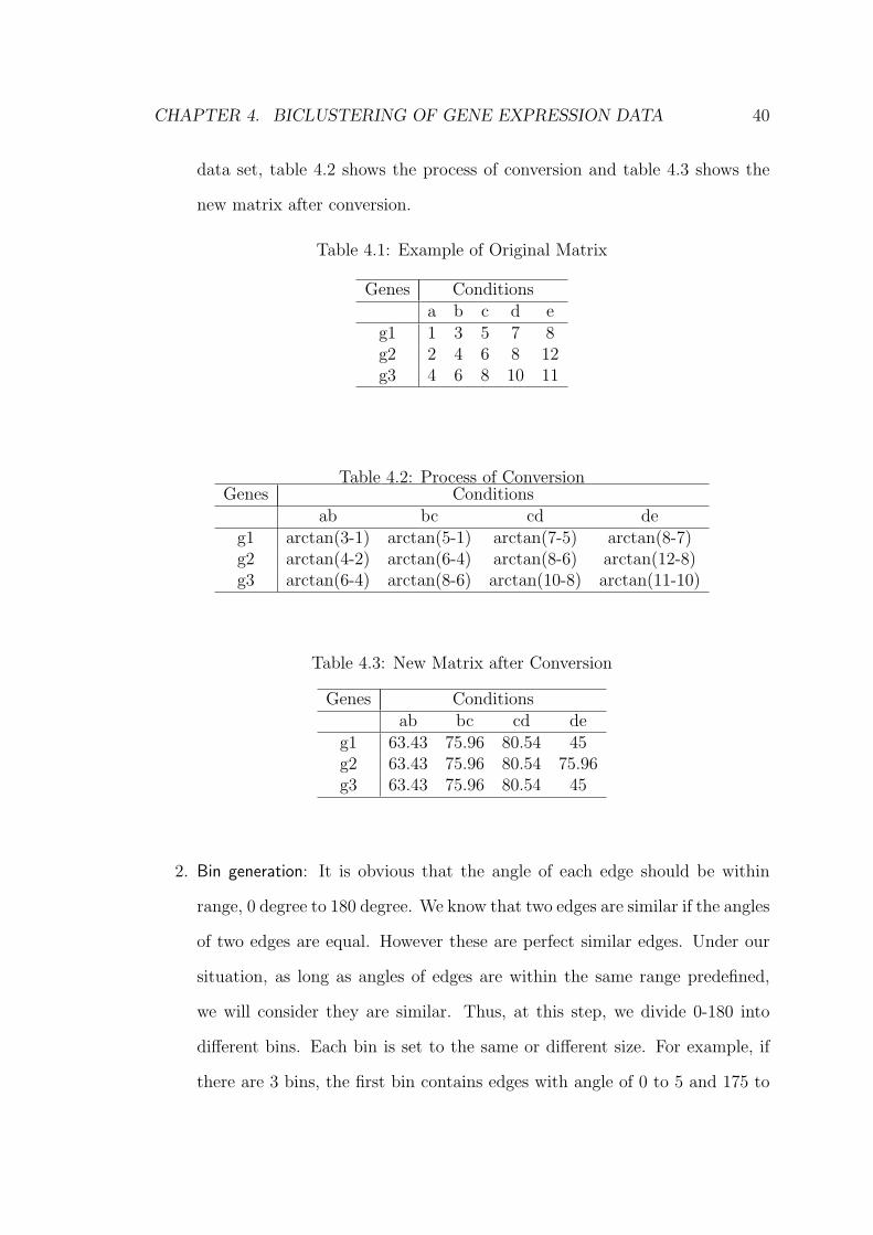
CHAPTER 4. BICLUSTERING OF GENE EXPRESSION DATA 41
0−5 or 175−180 5−9090−175
bin1bin2
bin3
Figure 4.1: Structure of Bins
180 degree. The second bin will contain edges whose angles are within the
range from 5 to 90 degree, and the third bin will contain edges whose angles
are within the range from 90 to 175 degree. Figure 4.1 shows structure of
bins. Each edge is represented by an integer, such as edge ’ab’ is represented
as 000, and ’bc’ is represented as 001 and so on. Then we scan through
the new matrix and put each edge into the corresponding bins according to
their angles. After this step, we can get a data set which contains changing
patterns of each gene under every two conditions. For example, if one row
contain a pattern, 301. It represents that one gene in a row has a changing
edge, ’bc’(001), in bin3. Table 4.4 is an example of final input data matrix
for frequent pattern mining.
Table 4.4: Input for Frequent Pattern Mining
Genes Conditionsab bc cd de
g1 200 201 202 203g2 200 201 202 203g3 200 201 202 203
4.4.2 Frequent Pattern Mining
In this step, we mine the new matrix data set from the last phase to find frequent
patterns. So far we have reduced good seeds (initial biclusters) of possible bicluster
problem to an ordinary problem of data mining, finding all frequent patterns. By
CHAPTER 4. BICLUSTERING OF GENE EXPRESSION DATA 42
0
2
4
6
8
10
12
14
16
a b c d e
expr
essi
on le
vel
condition
g1g2g3
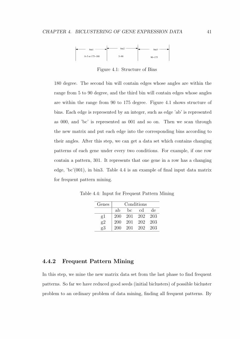
Figure 4.2: Original Data
definition, each of these patterns will occur at least as frequent as a pre-determined
minimum support count. Regarding our seeds finding problem, the minimum sup-
port count is actually the minimum support gene count, i.e. a particular pattern
appears in at least minimum number of genes. From these frequent patterns, it is
easy to extract good seeds of possible biclusters by converting edges back to origi-
nal conditions under a subset of genes. Figure 4.2 is an example of whole pattern
of data set. Then we will choose a data mining tool to mine this data set.
As mentioned, the mining tool we adopted in this work is CHARM. CHARM
was proposed by [ZH02], and has been shown to be an efficient algorithm for closed
itemset mining.
4.4.3 Extracting seeds of biclusters
This step extracts seeds of possible bicluster from the generated frequent patterns.
Basically, we need to convert the generated patterns back to the original conditions
as well as extract genes which contain these patterns. However, after extracting,
we can only get coarse seeds of possible biclusters, i.e. not all seeds’s mean squared
residue is less than the required threshold. In order to get refined seeds of biclusters,
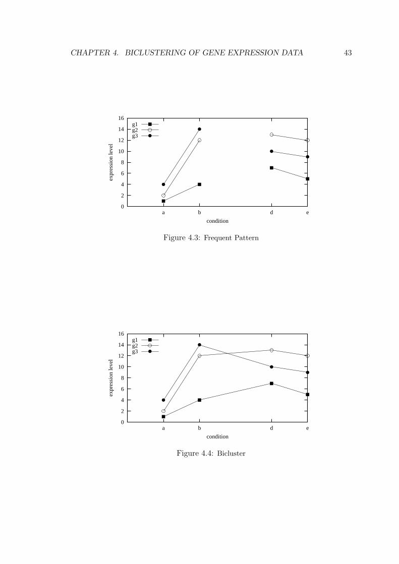
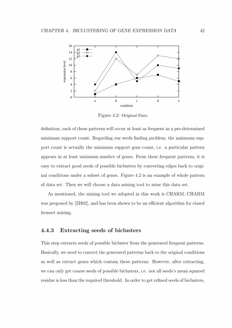
CHAPTER 4. BICLUSTERING OF GENE EXPRESSION DATA 43
0
2
4
6
8
10
12
14
16
a b d e
expr
essi
on le
vel
condition
g1g2g3
Figure 4.3: Frequent Pattern
0
2
4
6
8
10
12
14
16
a b d e
expr
essi
on le
vel
condition
g1g2g3
Figure 4.4: Bicluster

CHAPTER 4. BICLUSTERING OF GENE EXPRESSION DATA 44
we filter all coarse seeds we have gotten through a predefined threshold of mean
squared residue. For example, if we get a frequent pattern such as 300, 102, 303
in g1, g2, g3. After post processing,we know that g1, g2, g3 have edges,ab, de
with similar angles, just like the patttern in figure 4.3. Then we may consider the
pattern shown in figure 4.4 as a qualified bicluster seed if the mean squared residue
satisfies a predefined threshold, δ for some δ ≥ 0, otherwise, we will discard this
pattern, i.e we will not treat it as a good seed(bicluster).
Given that the number of patterns may be large (and hence the number of good
seeds is also large), we need to select only the best seeds. To facilitate this selection
process, we order the seeds based on the ratio of its residue over its volume, i.e.,
residuevolume
. The rationale for this metric is obvious: if the residue is smaller and/or the
volume is bigger,then the quality of a bicluster is better.
The algorithmic description of this phase is given in Algorithm 4.2. In the algo-
rithm, R() is mean square residue, the measurement of coherence of each bicluster.
The function for R() is given in equation 4.1. RowV ar() is row variance, by us-
ing it to eliminate trival biclusters whose changing trend is too flat. The function
for RowV ar()is given in equation 4.4. In the step 6, we use the ratio of ResidueV olume
to order biclusters we find, where Residue is the mean square residue (i.e.R()) of
final bicluster and V olume is the volume of a final bicluster which is obtained by
number of rows times number of columns in the final bicluster.
4.5 Phase 2: Node addition
At the end of the first phase, we have a set of good quality biclusters. However,
these biclusters may not be maximal, in other words, some rows and/or columns
may be added to increase their volume/size while keeping the mean squared residue
below the predetermined threshold δ. The reason is that some genes may be left out
CHAPTER 4. BICLUSTERING OF GENE EXPRESSION DATA 45
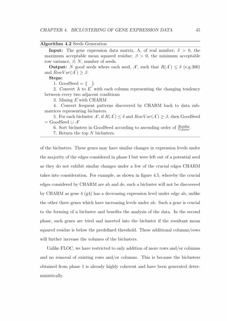
Algorithm 4.2 Seeds Generation
Input: The gene expression data matrix, A, of real number; δ > 0, themaximum acceptable mean squared residue; β > 0, the minimum acceptablerow variance, β; N , number of seeds.
Output: N good seeds where each seed, A′, such that R(A′) ≤ δ (e.g.300)
and RowV ar(A′) ≥ β.
Steps:1. GoodSeed = { }2. Convert A to E
′with each column representing the changing tendency
between every two adjacent conditions3. Mining E
′with CHARM
4. Convert frequent patterns discovered by CHARM back to data sub-matrices representing biclusters.
5. For each bicluster A′, if R(A′) ≤ δ and RowV ar(A
′) ≥ β, then GoodSeed
= GoodSeed ∪ A′
6. Sort biclusters in GoodSeed according to ascending order of ResidueV olume
.7. Return the top N biclusters.
of the biclusters. These genes may have similar changes in expression levels under
the majority of the edges considered in phase I but were left out of a potential seed
as they do not exhibit similar changes under a few of the crucial edges CHARM
takes into consideration. For example, as shown in figure 4.5, whereby the crucial
edges considered by CHARM are ab and de, such a bicluster will not be discovered
by CHARM as gene 4 (g4) has a decreasing expression level under edge ab, unlike
the other three genes which have increasing levels under ab. Such a gene is crucial
to the forming of a bicluster and benefits the analysis of the data. In the second
phase, such genes are tried and inserted into the bicluster if the resultant mean
squared residue is below the predefined threshold. These additional columns/rows
will further increase the volumes of the biclusters.
Unlike FLOC, we have restricted to only addition of more rows and/or columns
and no removal of existing rows and/or columns. This is because the biclusters
obtained from phase 1 is already highly coherent and have been generated deter-
ministically.

CHAPTER 4. BICLUSTERING OF GENE EXPRESSION DATA 46
Algorithm 4.3 Node Addition
Input: 100×M , M is a matrix of real number, I×J signifying a seed; residuethreshold δ > 0 (e.g.300); row variance threshold, β > 0.
Output:100 × M′, each M
′is a new matrix I
′ × J′
such that I ⊂ I′
andJ ⊂ J ′ with the property that Residue, R(M
′) ≤ δ and RowV ar(M
′) > β.
Iteration:From M1 to M100 do:
1. Compute gainj for all columns, j /∈ J2. Sort gainj in descending order3. Find columns j /∈ J starting from the one with the most gain, GjintoM ,
such that the residue score of new bicluster of after inserting j into M, R(M′)
≤ δ and GjintoM≥ previous highest gain, GjintoM” if j has been inserted intoother bilcuster M” before and row variance of new bicluster RowV ar(M
′) > β.
4. If j is not empty (i.e., M can be extended with column j), M′
=insertColumn(M , j).
5. Compute gaini for all rows, i /∈ I6. Sort gaini in descending order7. Find rows i /∈ I starting from the one with the most gain, GiintoM , such
that the residue score of new bicluster of after inserting i into M, R(M′) ≤ δ
and GiintoM≥ previous highest gain, GiintoM” if i has been inserted into otherbilcuster M” before and row variance of new bicluster RowV ar(M
′) > β.
8. If i is not empty (i.e., M can be extended with row i), M′
= in-sertRow(M, i).
9.Reset the highest gains for the columns and rows to zero for the nextiteration.
10. If nothing is added, return I and J as I′and J
′.

CHAPTER 4. BICLUSTERING OF GENE EXPRESSION DATA 47
Figure 4.5: Possible Seeds Discovered by CHARM
The second phase is an iterative process to improve the quality of the biclusters
discovered in the first phase. The purpose is to increase the volume of the biclusters.
During each iteration, each bicluster is repeatedly tested with columns and rows
not included in it to determine if they can be included. The concept of gain in
FLOC [YWWY03] is used here.
Definition 1 Given a residue threshold δ, the gain of inserting a column/row x
into a bicluster c is defined as Gain(x, c) =rc−rc′
r2
rc
+vc′−vc
vcwhere rc, rc′ are the
residues of bicluster c and bicluster c′, obtained by performing the insertion, re-
specitvely and vc and vc′ are the volumes fo c and c′, respectively.
At each iteration, the gains of inserting columns/rows that are not included in
each particular initial bicluster are calculated and sorted in a descending order. All
gains are calculated with respect to the original bicluster in each iteration. Then
a insertion of a column/row is only carried out when all of the following three
conditions are satisfied:
1. The column/row is inserted only when the mean squared residue of the new
bicluster M′
obtained after the insertion of a column/row is less than the
predetermined threshold value.

CHAPTER 4. BICLUSTERING OF GENE EXPRESSION DATA 48
2. Either the column/row never be inserted to other biclusters before or the gain
of inserting the column/row into the current bicluster is larger than or equal
to the previous highest value for the gain of inserting this column/row into
other previous biclusters in this iteration. This gain is different from the gain
using for sorting. It is calculated with respect to the latest bicluster. After
each iteration, the highest value for the gain of the each possible inserting
column/row is set to zero to prepare for the next iteration.
3. The resultant addition results in the bicluster having a row variance that is
bigger than a predefined value.
For example, in one iteration, one seed, M3 has 3 possible conditions, C1, C2,
C3 can be inserted into M3. The gain with respect to M3 for these three conditions
are Gain1, Gain2, Gain3. After sorting, the order for three gains are Gain3,
Gain1, Gain2. So we will see C3 first, the residue of new biclsuter after inserting
C3 into M3 is M′3, and R(M
′3 ≥ 300; then we check if C3 has been inserted to other
biclusters before, either C3 is used here for the first time or G3 ≥ G3′which is the
gain when C3 is inserted in other bicluster previously in this iteration, then we will
check the row variance after inserting C3 into M3, if RowV ar(M3′) ≥ 100, then
we will insert C3 into M3. If any one of these three conditions is not satisfied, we
will proceed to see the next possible condition C1 which has the second biggest
gain in the sorting list. This process will continue until all possible conditions for
this bicluster are considered, then the algorithm will proceed to the next seeds, and
so on until finishing all 100 seeds, the biggest gain for each condition is set to 0, and
the algorithm starts another iteration, when there is not any improvement for all
100 seeds, the iteration will stop. The same will be performed for adding rows. We
choose 300 as threshold for mean square residue and 100 as the threshold of row
variance according to previous studies in this area, such as [CC00] and [YWWY03]

CHAPTER 4. BICLUSTERING OF GENE EXPRESSION DATA 49
Algorithm 4.3 presents the algorithmic description of this phase.
4.6 Adding Deletion in Phase 2
In designing DBF, we expect the seeds generated in the first phase to be good. As
such, we do not expect the second phase to have node deletion. However, in order
to validate that the seeds produced from the first phase are optimal, we also add
deletion in the second phase to see if there are any improvement in the quality of
final bicluster we get.
The Experiment 2 result in section 4.7.2 shows that deletion does not improve
quality of biclusters with respect to the small residue and big volume, however it
can reduce some overlaps among biclusters found by DBF. The algorithm of second
phase after adding deletion is shown in algorithm 4.4.
Node deletion is carried out at the end of every iteration. Here, DBF will
look for columns/rows that were inserted in that iteration and take the average
of the highest and lowest positive gains for each of them. These gain values are
the actual gain values of inserting that particular column/row into some biclusters
in that iteration. Let these average values be known as AvGains. Next, for each
column/row that was inserted in that iteration, DBF will look for all the biclusters
that contain it and calculate the gains of deleting it from those biclusters. If
these gains are greater than the AvGain corresponding to that column/row, that
column/row will be deleted from these biclusters.
AvGain is used here instead of the highest gain associated with the particular
column as more biclusters can benefit from the deletion of such columns. The
benefits they gained from the reductions in their residue values far outweigh the loss
from having volume reductions. This is also done in order to reduce the redundant
overlapping among biclusters i.e. finally each column/row is only contained in the
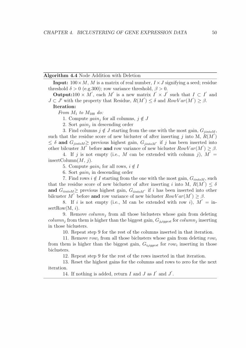
CHAPTER 4. BICLUSTERING OF GENE EXPRESSION DATA 50
Algorithm 4.4 Node Addition with Deletion
Input: 100×M , M is a matrix of real number, I×J signifying a seed; residuethreshold δ > 0 (e.g.300); row variance threshold, β > 0.
Output:100 × M′, each M
′is a new matrix I
′ × J′
such that I ⊂ I′
andJ ⊂ J ′ with the property that Residue, R(M
′) ≤ δ and RowV ar(M
′) ≥ β.
Iteration:From M1 to M100 do:
1. Compute gainj for all columns, j /∈ J2. Sort gainj in descending order3. Find columns j /∈ J starting from the one with the most gain, GjintoM ,
such that the residue score of new bicluster of after inserting j into M, R(M′)
≤ δ and GjintoM≥ previous highest gain, GjintoM” if j has been inserted intoother bilcuster M” before and row variance of new bicluster RowV ar(M
′) ≥ β.
4. If j is not empty (i.e., M can be extended with column j), M′
=insertColumn(M , j).
5. Compute gaini for all rows, i /∈ I6. Sort gaini in descending order7. Find rows i /∈ I starting from the one with the most gain, GiintoM , such
that the residue score of new bicluster of after inserting i into M, R(M′) ≤ δ
and GiintoM≥ previous highest gain, GiintoM” if i has been inserted into otherbilcuster M” before and row variance of new bicluster RowV ar(M
′) ≥ β.
8. If i is not empty (i.e., M can be extended with row i), M′
= in-sertRow(M, i).
9. Remove columnj from all those biclusters whose gain from deletingcolumnj from them is higher than the biggest gain, Gjbiggest for columnj insertingin those biclusters.
10. Repeat step 9 for the rest of the columns inserted in that iteration.11. Remove rowi from all those biclusters whose gain from deleting rowi
from them is higher than the biggest gain, Gibiggest for rowi inserting in thosebiclusters.
12. Repeat step 9 for the rest of the rows inserted in that iteration.13. Reset the highest gains for the columns and rows to zero for the next
iteration.14. If nothing is added, return I and J as I
′and J
′.
CHAPTER 4. BICLUSTERING OF GENE EXPRESSION DATA 51
biclusters which will benefit greatly from it in terms of lower residues or bigger
volumes. Also, if the deletion of a column/row will result in a bicluster having a
row variance lesser than or equal to , the action will not be performed.
4.7 Experimental Study
We implemented the proposed DBF algorithm in C/C++ programming language.
For comparison, we also implemented FLOC. We also evaluated against a vari-
ation of FLOC that employs the results of the first phase of DBF as the ini-
tial clusters to FLOC’s second phase. We conducted all experiments on a sin-
gle node (comprising a dual 2.8GHz Intel Pentium 4 with 2.5GB RAM) of a
90-node Unix-based cluster. We use the Yeast microarray data set downloaded
from http://cheng.ececs.uc.edu/biclustering/yeast.matrix. The data set is based
on Tavazoie et al.[THC+99], and contains 2884 genes and 17 conditions. So the
data is a matrix with 2884 rows and 17 columns, 4 bytes for each element, with -1
indicating a missing value.
The genes were identified by SGD ORF names[BDD+00]. The relative abun-
dance values were taken from a table prepared by Aach, J. et al.[ARC00].
Data set download from http://cheng.ececs.uc.edu/biclustering/lymphoma.matrix
is also used in our experimental study. This data set is Human Gene Expression
data based on Alizadeh et al [AED+00]. It is a a matrix with 4026 rows and 96
columns, 4 bytes for each element, and 999 indicating a missing value.
4.7.1 Experiment 1
We have conducted a large number of experiments. Our results show that DBF is
able to locate larger biclusters with smaller residue. This is because our algorithm
can discover more highly coherent genes and conditions which leads to smaller
CHAPTER 4. BICLUSTERING OF GENE EXPRESSION DATA 52
mean squared residue. Meanwhile the final biclusters generated by our algorithm
is deterministic whereas those produced by FLOC is non-deterministic Moreover,
the quality of the final biclusters can not be guaranteed by FLOC: the residue and
size of the final biclusters found by FLOC varies greatly and is highly dependent on
the initial seeds. Here, we shall present some representative results. In particular,
both algorithms are used to find 100 biclusters whose residue is less than 300. For
DBF, the default support value is 0.03.
We first present the results on comparing DBF with the original FLOC scheme.
Figure 4.6 shows the frequency distribution of residues of 100 biclusters obtained
by DBF and FLOC respectively. Figure 4.7 shows the distribution of the sizes
(volume) of the 100 biclusters obtained by DBF and FLOC respectively. As the
sizes of seeds used in the first phase of FLOC are random, we test it with five
cases: in the first case, initial biclusters are 2 (genes) by 4 (conditions) in size, in
the second case, they are 2(genes) by 7(conditions), in the third case they are 2
(genes) by 9 (conditions), in the fourth case they are 80 by 6 and the fifth they
are 144(genes) by 6(conditons) . However, the output for fourth and fifth cases are
the random seeds itself, i.e. the second phase of FLOC did not improve them at
all, so we only show the first to the third cases here for FLOC. From figure 4.6, we
observe that more than half of the final biclusters found by DBF has residues in
the range of 150-200 and all biclusters found by DBF have residues smaller than
225. Meanwhile (see figure 4.7), more than 50% of the 100 biclusters’ sizes found
by DBF fall within the 2000-3000 range. On the other hand, for FLOC, the final
resultant biclusters are very much dependent on the initial random seeds. Such as
in the case of 2 genes by 4 conditions, most of the volumes of the final biclusters
are very small and are less than 500 although their residues are small. As for
the other two sets of initial seeds having 2 genes by 7 conditions and 2 genes by 9
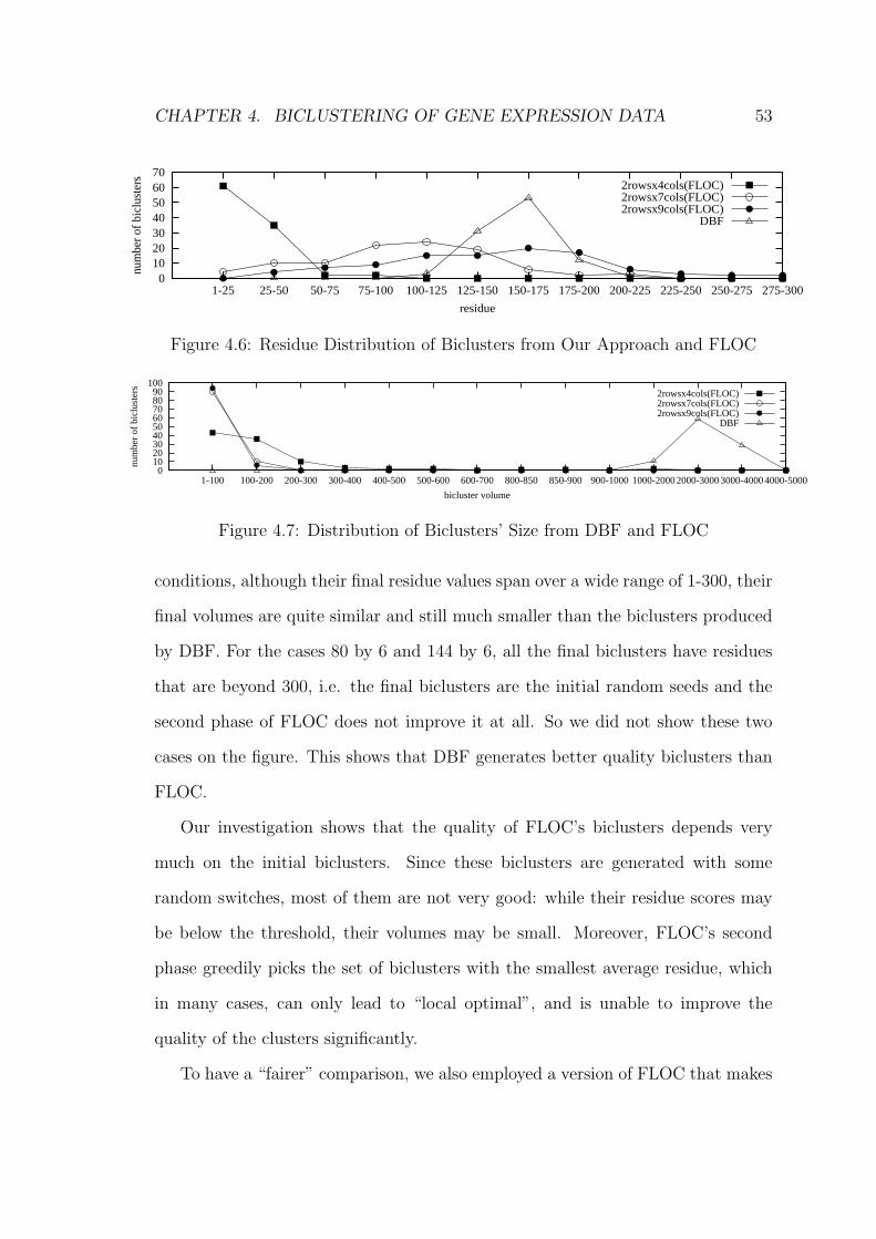
CHAPTER 4. BICLUSTERING OF GENE EXPRESSION DATA 53
010203040506070
1-25 25-50 50-75 75-100 100-125 125-150 150-175 175-200 200-225 225-250 250-275 275-300
num
ber
of b
iclu
ster
s
residue
2rowsx4cols(FLOC)2rowsx7cols(FLOC)2rowsx9cols(FLOC)
DBF
Figure 4.6: Residue Distribution of Biclusters from Our Approach and FLOC
0102030405060708090
100
1-100 100-200 200-300 300-400 400-500 500-600 600-700 800-850 850-900 900-1000 1000-2000 2000-3000 3000-4000 4000-5000
num
ber
of b
iclu
ster
s
bicluster volume
2rowsx4cols(FLOC)2rowsx7cols(FLOC)2rowsx9cols(FLOC)
DBF
Figure 4.7: Distribution of Biclusters’ Size from DBF and FLOC
conditions, although their final residue values span over a wide range of 1-300, their
final volumes are quite similar and still much smaller than the biclusters produced
by DBF. For the cases 80 by 6 and 144 by 6, all the final biclusters have residues
that are beyond 300, i.e. the final biclusters are the initial random seeds and the
second phase of FLOC does not improve it at all. So we did not show these two
cases on the figure. This shows that DBF generates better quality biclusters than
FLOC.
Our investigation shows that the quality of FLOC’s biclusters depends very
much on the initial biclusters. Since these biclusters are generated with some
random switches, most of them are not very good: while their residue scores may
be below the threshold, their volumes may be small. Moreover, FLOC’s second
phase greedily picks the set of biclusters with the smallest average residue, which
in many cases, can only lead to “local optimal”, and is unable to improve the
quality of the clusters significantly.
To have a “fairer” comparison, we also employed a version of FLOC that makes
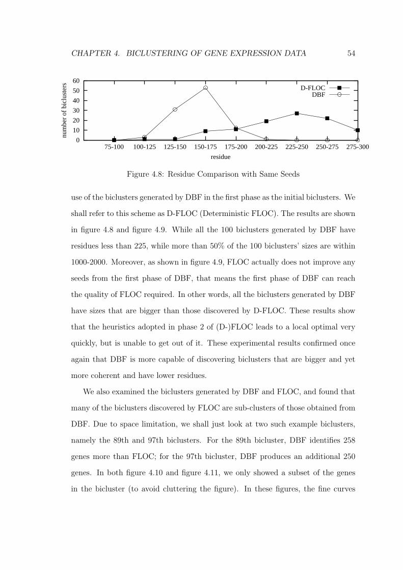
CHAPTER 4. BICLUSTERING OF GENE EXPRESSION DATA 54
0
10
20
30
40
50
60
75-100 100-125 125-150 150-175 175-200 200-225 225-250 250-275 275-300
num
ber
of b
iclu
ster
s
residue
D-FLOCDBF
Figure 4.8: Residue Comparison with Same Seeds
use of the biclusters generated by DBF in the first phase as the initial biclusters. We
shall refer to this scheme as D-FLOC (Deterministic FLOC). The results are shown
in figure 4.8 and figure 4.9. While all the 100 biclusters generated by DBF have
residues less than 225, while more than 50% of the 100 biclusters’ sizes are within
1000-2000. Moreover, as shown in figure 4.9, FLOC actually does not improve any
seeds from the first phase of DBF, that means the first phase of DBF can reach
the quality of FLOC required. In other words, all the biclusters generated by DBF
have sizes that are bigger than those discovered by D-FLOC. These results show
that the heuristics adopted in phase 2 of (D-)FLOC leads to a local optimal very
quickly, but is unable to get out of it. These experimental results confirmed once
again that DBF is more capable of discovering biclusters that are bigger and yet
more coherent and have lower residues.
We also examined the biclusters generated by DBF and FLOC, and found that
many of the biclusters discovered by FLOC are sub-clusters of those obtained from
DBF. Due to space limitation, we shall just look at two such example biclusters,
namely the 89th and 97th biclusters. For the 89th bicluster, DBF identifies 258
genes more than FLOC; for the 97th bicluster, DBF produces an additional 250
genes. In both figure 4.10 and figure 4.11, we only showed a subset of the genes
in the bicluster (to avoid cluttering the figure). In these figures, the fine curves
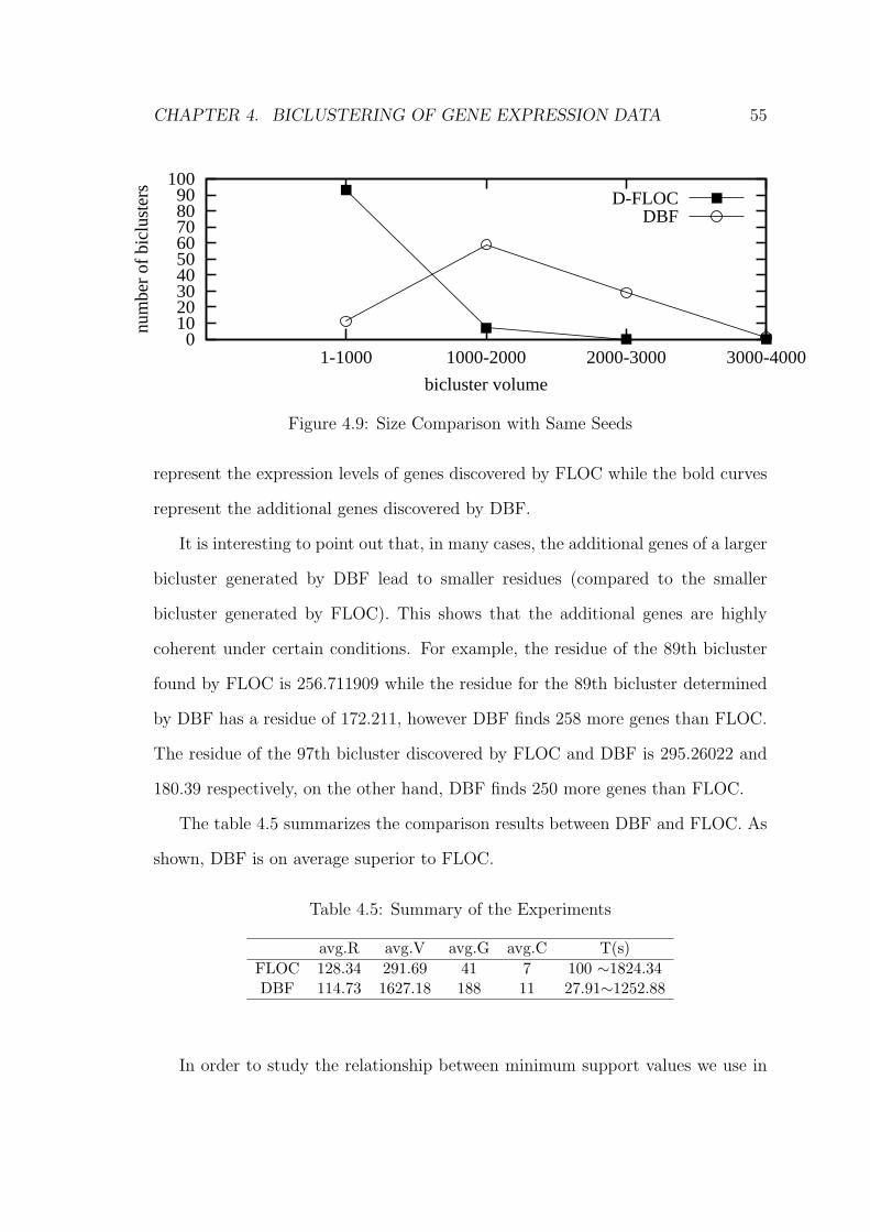
CHAPTER 4. BICLUSTERING OF GENE EXPRESSION DATA 55
0102030405060708090
100
1-1000 1000-2000 2000-3000 3000-4000
num
ber
of b
iclu
ster
s
bicluster volume
D-FLOCDBF
Figure 4.9: Size Comparison with Same Seeds
represent the expression levels of genes discovered by FLOC while the bold curves
represent the additional genes discovered by DBF.
It is interesting to point out that, in many cases, the additional genes of a larger
bicluster generated by DBF lead to smaller residues (compared to the smaller
bicluster generated by FLOC). This shows that the additional genes are highly
coherent under certain conditions. For example, the residue of the 89th bicluster
found by FLOC is 256.711909 while the residue for the 89th bicluster determined
by DBF has a residue of 172.211, however DBF finds 258 more genes than FLOC.
The residue of the 97th bicluster discovered by FLOC and DBF is 295.26022 and
180.39 respectively, on the other hand, DBF finds 250 more genes than FLOC.
The table 4.5 summarizes the comparison results between DBF and FLOC. As
shown, DBF is on average superior to FLOC.
Table 4.5: Summary of the Experiments
avg.R avg.V avg.G avg.C T(s)FLOC 128.34 291.69 41 7 100 ∼1824.34DBF 114.73 1627.18 188 11 27.91∼1252.88
In order to study the relationship between minimum support values we use in
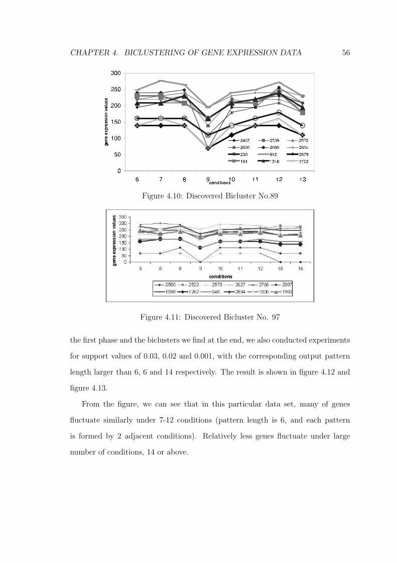
CHAPTER 4. BICLUSTERING OF GENE EXPRESSION DATA 56
Figure 4.10: Discovered Bicluster No.89
Figure 4.11: Discovered Bicluster No. 97
the first phase and the biclusters we find at the end, we also conducted experiments
for support values of 0.03, 0.02 and 0.001, with the corresponding output pattern
length larger than 6, 6 and 14 respectively. The result is shown in figure 4.12 and
figure 4.13.
From the figure, we can see that in this particular data set, many of genes
fluctuate similarly under 7-12 conditions (pattern length is 6, and each pattern
is formed by 2 adjacent conditions). Relatively less genes fluctuate under large
number of conditions, 14 or above.
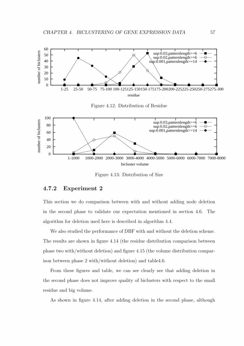
CHAPTER 4. BICLUSTERING OF GENE EXPRESSION DATA 57
0
10
20
30
40
50
60
1-25 25-50 50-75 75-100 100-125125-150150-175175-200200-225225-250250-275275-300
num
ber
of b
iclu
ster
s
residue
sup:0.03,patternlength>=6sup:0.02,patternlength>=6
sup:0.001,patternlength>=14
Figure 4.12: Distribution of Residue
0
20
40
60
80
100
1-1000 1000-2000 2000-3000 3000-4000 4000-5000 5000-6000 6000-7000 7000-8000
num
ber
of b
iclu
ster
s
bicluster volume
sup:0.03,patternlength>=6sup:0.02,patternlength>=6
sup:0.001,patternlength>=14
Figure 4.13: Distribution of Size
4.7.2 Experiment 2
This section we do comparison between with and without adding node deletion
in the second phase to validate our expectation mentioned in section 4.6. The
algorithm for deletion used here is described in algorithm 4.4.
We also studied the performance of DBF with and without the deletion scheme.
The results are shown in figure 4.14 (the residue distribution comparison between
phase two with/without deletion) and figure 4.15 (the volume distribution compar-
ison between phase 2 with/without deletion) and table4.6.
From these figures and table, we can see clearly see that adding deletion in
the second phase does not improve quality of biclusters with respect to the small
residue and big volume.
As shown in figure 4.14, after adding deletion in the second phase, although
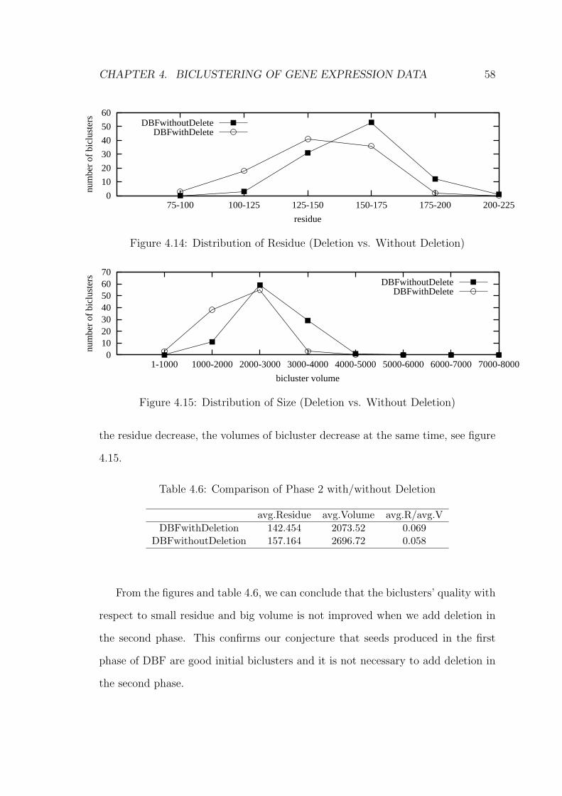
CHAPTER 4. BICLUSTERING OF GENE EXPRESSION DATA 58
0
10
20
30
40
50
60
75-100 100-125 125-150 150-175 175-200 200-225
num
ber
of b
iclu
ster
s
residue
DBFwithoutDeleteDBFwithDelete
Figure 4.14: Distribution of Residue (Deletion vs. Without Deletion)
010203040506070
1-1000 1000-2000 2000-3000 3000-4000 4000-5000 5000-6000 6000-7000 7000-8000
num
ber
of b
iclu
ster
s
bicluster volume
DBFwithoutDeleteDBFwithDelete
Figure 4.15: Distribution of Size (Deletion vs. Without Deletion)
the residue decrease, the volumes of bicluster decrease at the same time, see figure
4.15.
Table 4.6: Comparison of Phase 2 with/without Deletion
avg.Residue avg.Volume avg.R/avg.VDBFwithDeletion 142.454 2073.52 0.069
DBFwithoutDeletion 157.164 2696.72 0.058
From the figures and table 4.6, we can conclude that the biclusters’ quality with
respect to small residue and big volume is not improved when we add deletion in
the second phase. This confirms our conjecture that seeds produced in the first
phase of DBF are good initial biclusters and it is not necessary to add deletion in
the second phase.
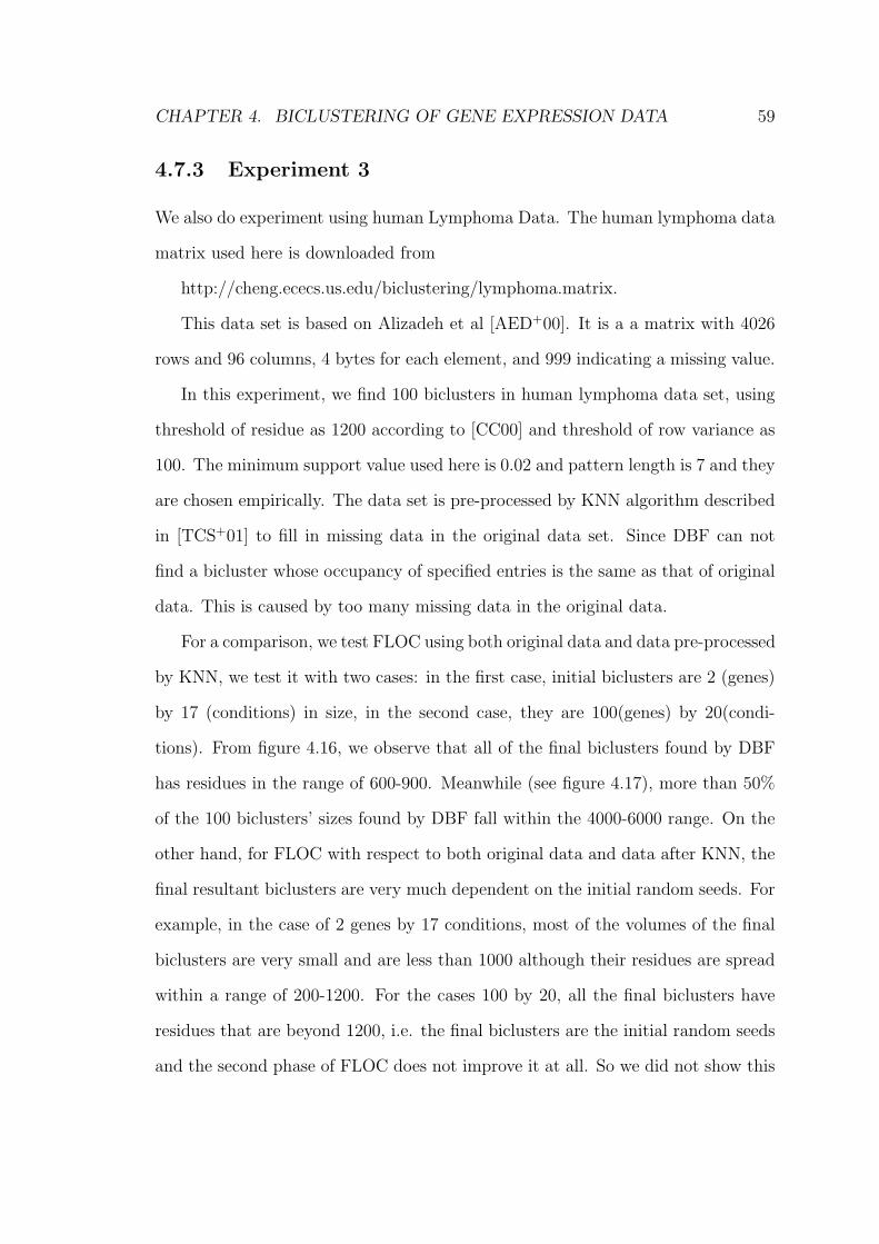
CHAPTER 4. BICLUSTERING OF GENE EXPRESSION DATA 59
4.7.3 Experiment 3
We also do experiment using human Lymphoma Data. The human lymphoma data
matrix used here is downloaded from
http://cheng.ececs.us.edu/biclustering/lymphoma.matrix.
This data set is based on Alizadeh et al [AED+00]. It is a a matrix with 4026
rows and 96 columns, 4 bytes for each element, and 999 indicating a missing value.
In this experiment, we find 100 biclusters in human lymphoma data set, using
threshold of residue as 1200 according to [CC00] and threshold of row variance as
100. The minimum support value used here is 0.02 and pattern length is 7 and they
are chosen empirically. The data set is pre-processed by KNN algorithm described
in [TCS+01] to fill in missing data in the original data set. Since DBF can not
find a bicluster whose occupancy of specified entries is the same as that of original
data. This is caused by too many missing data in the original data.
For a comparison, we test FLOC using both original data and data pre-processed
by KNN, we test it with two cases: in the first case, initial biclusters are 2 (genes)
by 17 (conditions) in size, in the second case, they are 100(genes) by 20(condi-
tions). From figure 4.16, we observe that all of the final biclusters found by DBF
has residues in the range of 600-900. Meanwhile (see figure 4.17), more than 50%
of the 100 biclusters’ sizes found by DBF fall within the 4000-6000 range. On the
other hand, for FLOC with respect to both original data and data after KNN, the
final resultant biclusters are very much dependent on the initial random seeds. For
example, in the case of 2 genes by 17 conditions, most of the volumes of the final
biclusters are very small and are less than 1000 although their residues are spread
within a range of 200-1200. For the cases 100 by 20, all the final biclusters have
residues that are beyond 1200, i.e. the final biclusters are the initial random seeds
and the second phase of FLOC does not improve it at all. So we did not show this
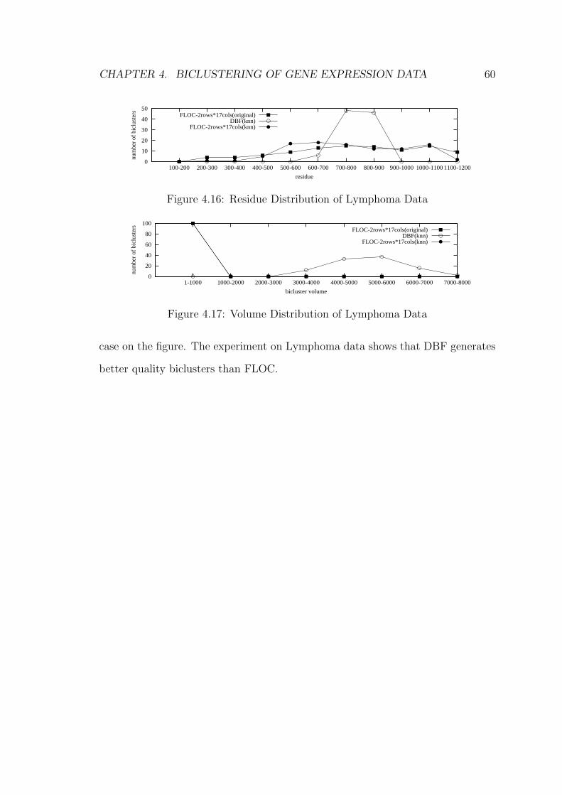
CHAPTER 4. BICLUSTERING OF GENE EXPRESSION DATA 60
0
10
20
30
40
50
100-200 200-300 300-400 400-500 500-600 600-700 700-800 800-900 900-1000 1000-1100 1100-1200
num
ber
of b
iclu
ster
s
residue
FLOC-2rows*17cols(original)DBF(knn)
FLOC-2rows*17cols(knn)
Figure 4.16: Residue Distribution of Lymphoma Data
0
20
40
60
80
100
1-1000 1000-2000 2000-3000 3000-4000 4000-5000 5000-6000 6000-7000 7000-8000
num
ber
of b
iclu
ster
s
bicluster volume
FLOC-2rows*17cols(original)DBF(knn)
FLOC-2rows*17cols(knn)
Figure 4.17: Volume Distribution of Lymphoma Data
case on the figure. The experiment on Lymphoma data shows that DBF generates
better quality biclusters than FLOC.
Chapter 5
Gene Selection for classification
Gene expression data presents special challenges for discriminant analysis as the
number of genes is very large compared to the number of samples. However, in
most cases only a small fraction of these genes that may reveal the important
biological process. Moreover, there is not only a danger of the irrelevant genes
covering up the contributions of the relevant ones but also there is a computational
burden. Hence, gene selection is an important issue in microarray data analysis
and the significance of finding the minimum gene subset is obvious. First it can
greatly reduces the computational burden and ”noise” arising from irrelevant genes.
Second, it simplifies gene expression tests to include only a very small number of
genes rather than thousands of genes. Third it calls further investigations into
possible biological relationship between these small number of genes and cancer
development and treatment. In this chapter we proposed a simple method to find
a small subset of genes that can classify type of cancers almost perfectly using
supervised learning.
61
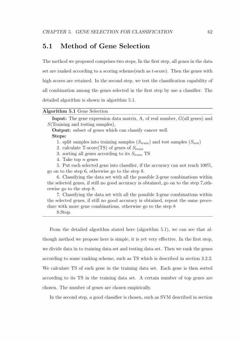
CHAPTER 5. GENE SELECTION FOR CLASSIFICATION 62
5.1 Method of Gene Selection
The method we proposed comprises two steps, In the first step, all genes in the data
set are ranked according to a scoring scheme(such as t-score). Then the genes with
high scores are retained. In the second step, we test the classification capability of
all combination among the genes selected in the first step by use a classifier. The
detailed algorithm is shown in algorithm 5.1.
Algorithm 5.1 Gene Selection
Input: The gene expression data matrix, A, of real number, G(all genes) andS(Training and testing samples),
Output: subset of genes which can classify cancer well.Steps:
1. split samples into training samples (Strain) and test samples (Stest)2. calculate T-score(TS) of genes of Strain
3. sorting all genes according to its Strain TS4. Take top n genes5. Put each selected gene into classifier, if the accuracy can not reach 100%,
go on to the step 6, otherwise go to the step 8.6. Classifying the data set with all the possible 2-gene combinations within
the selected genes, if still no good accuracy is obtained, go on to the step 7,oth-erwise go to the step 8.
7. Classifying the data set with all the possible 3-gene combinations withinthe selected genes, if still no good accuracy is obtained, repeat the same proce-dure with more gene combinations, otherwise go to the step 8
8.Stop.
From the detailed algorithm stated here (algorithm 5.1), we can see that al-
though method we propose here is simple, it is yet very effective. In the first step,
we divide data in to training data set and testing data set. Then we rank the genes
according to some ranking scheme, such as TS which is described in section 3.2.2.
We calculate TS of each gene in the training data set. Each gene is then sorted
according to its TS in the training data set. A certain number of top genes are
chosen. The number of genes are chosen empirically.
In the second step, a good classifier is chosen, such as SVM described in section
CHAPTER 5. GENE SELECTION FOR CLASSIFICATION 63
3.3.3. Train the classifier using training data set. Followed by testing the classifier
with testing data set.
Actually this is just an exhaustive search to see effects of combination of top
genes in the TS ranking for a classifier.
At first, each one of top genes got in the first step is treated as a single feature
respectively. Then we train the classifier with training data set with this one
feature, then test the trained classifier with testing data set. If the testing result
is good (i.e. the accuracy reaches 100%), the training and testing process will
stop. Otherwise, if the testing accuracy is not good (i.e. the accuracy can not
reach 100%) , every two combination among the top genes are treated as two
features respectively and the classifier is trained again using training data set with
two features, then test the trained classifier with testing data set. If the testing
accuracy is still not good, every three combination within the top gene rank list
will be treated as three features respectively and repeat the previous step again
and so on until the testing result is good.
5.2 Experiment
In the experiment, three sets of data are chosen. They are Lymphoma data[AED+00]
which is obtained from (http://llmpp.nih.gov/lymphoma), SRBCT data[KWR+01]
obtained from (http://research.nhgri.nih.gov/microarray/Supplement) and Liver
Cancer data[CCS+02] obtained from (http://genome-www.standford.edu/hcc/).
In the Lymphoma data set, there are 42 samples derived from diffuse large B-cell
lymphoma (DLBCL), 9 samples from follicular lymphoma(FL), 11 samples from
chronic lymphocytic leukaemia (CLL). The entire data set includes the expression
data of 4026 genes.
In the SRBCT data set, the entire data set contains the expression data of 2308
CHAPTER 5. GENE SELECTION FOR CLASSIFICATION 64
genes. There are totally 63 training samples and 25 testing samples provided, 5 of
the testing samples are not SRBCTs. The 63 training samples contains 23 Ewing
family of tumors (EWS), 20 rhabdomyosarcoma (RMS), 12 neuroblastoma (NB),
and 8 Burkitt lymphomas (BL). And the 20 SRBCT testing samples contain 6
EWA, 5 RWS, 6 NB, and 3 BL.
In Liver Cancer data set, there are 1648 genes. The data set contains 156
samples. Among them, 82 are HCCs and the other 74 are non-tumor livers.
For all data sets, if there are any missing data, k-nearest neighbor method will
be used to fill those missing values [TCS+01].
We rank all genes in each data set by TS. According to TS, we chose 196
important genes from Lymphoma data, 30 important genes from SRBCT data set,
and 150 important genes liver cancer data set.
The classifier we used here is C-SVM with radial basis kernel functions. It is
contained in LIBSVM down load from http://www.csie.ntu.edu.tw/ cjlin/libsvm/.
A ”one-against-one” scheme [CL02] is used to group the binary SVMs to solve
multi-class problems. Parameters of the SVM are default in LIBSVM.
We first divide each data set randomly into training data samples and test data
set, such as for Lymphoma data set, there are 31 training samples and 31 testing
samples, for SRBCT data set, there are 63 training samples and 25 testing samples,
and for Liver cancer data set, there are 93 training samples and 63 testing samples.
Then we applied SVM to these three data sets. We train and test SVM with each
one of genes in selected ranking genes, if the the accuracy is not good, we repeat this
process with all possible combination of two genes in the selected ranking genes, if
the result is not satisfactory, we repeat the process with all possible combinations
of 3 genes in the selected ranking genes, and so on. We train all the training sample
using left-one-out cross validation to validate the results.
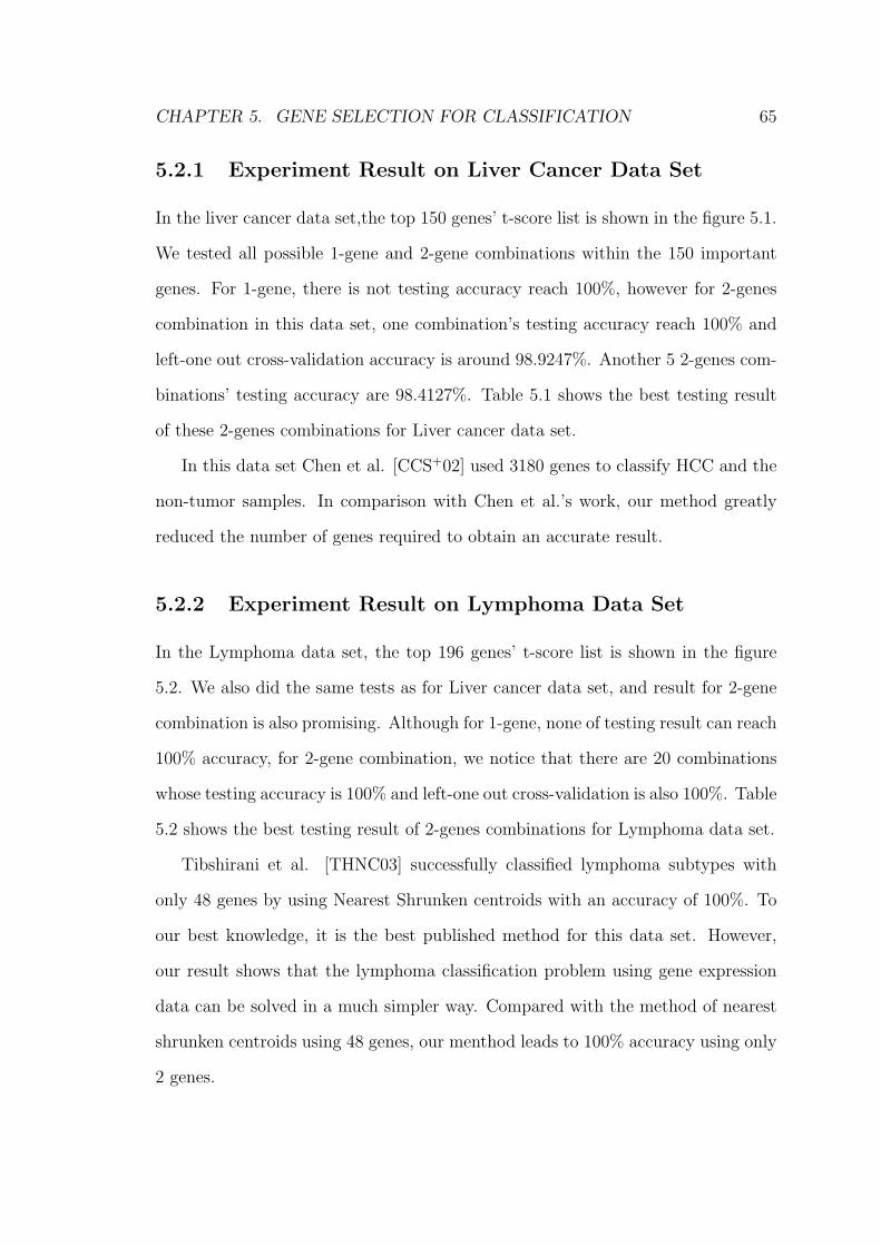
CHAPTER 5. GENE SELECTION FOR CLASSIFICATION 65
5.2.1 Experiment Result on Liver Cancer Data Set
In the liver cancer data set,the top 150 genes’ t-score list is shown in the figure 5.1.
We tested all possible 1-gene and 2-gene combinations within the 150 important
genes. For 1-gene, there is not testing accuracy reach 100%, however for 2-genes
combination in this data set, one combination’s testing accuracy reach 100% and
left-one out cross-validation accuracy is around 98.9247%. Another 5 2-genes com-
binations’ testing accuracy are 98.4127%. Table 5.1 shows the best testing result
of these 2-genes combinations for Liver cancer data set.
In this data set Chen et al. [CCS+02] used 3180 genes to classify HCC and the
non-tumor samples. In comparison with Chen et al.’s work, our method greatly
reduced the number of genes required to obtain an accurate result.
5.2.2 Experiment Result on Lymphoma Data Set
In the Lymphoma data set, the top 196 genes’ t-score list is shown in the figure
5.2. We also did the same tests as for Liver cancer data set, and result for 2-gene
combination is also promising. Although for 1-gene, none of testing result can reach
100% accuracy, for 2-gene combination, we notice that there are 20 combinations
whose testing accuracy is 100% and left-one out cross-validation is also 100%. Table
5.2 shows the best testing result of 2-genes combinations for Lymphoma data set.
Tibshirani et al. [THNC03] successfully classified lymphoma subtypes with
only 48 genes by using Nearest Shrunken centroids with an accuracy of 100%. To
our best knowledge, it is the best published method for this data set. However,
our result shows that the lymphoma classification problem using gene expression
data can be solved in a much simpler way. Compared with the method of nearest
shrunken centroids using 48 genes, our menthod leads to 100% accuracy using only
2 genes.
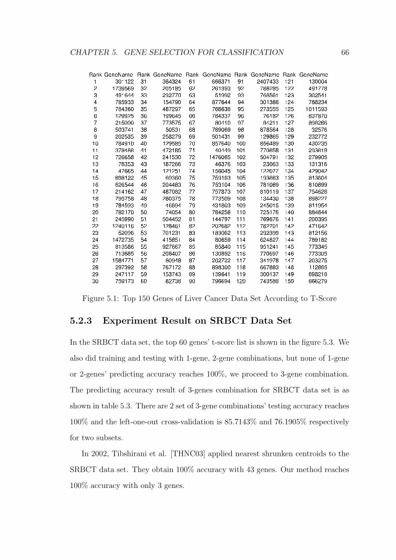
CHAPTER 5. GENE SELECTION FOR CLASSIFICATION 66
Figure 5.1: Top 150 Genes of Liver Cancer Data Set According to T-Score
5.2.3 Experiment Result on SRBCT Data Set
In the SRBCT data set, the top 60 genes’ t-score list is shown in the figure 5.3. We
also did training and testing with 1-gene, 2-gene combinations, but none of 1-gene
or 2-genes’ predicting accuracy reaches 100%, we proceed to 3-gene combination.
The predicting accuracy result of 3-genes combination for SRBCT data set is as
shown in table 5.3. There are 2 set of 3-gene combinations’ testing accuracy reaches
100% and the left-one-out cross-validation is 85.7143% and 76.1905% respectively
for two subsets.
In 2002, Tibshirani et al. [THNC03] applied nearest shrunken centroids to the
SRBCT data set. They obtain 100% accuracy with 43 genes. Our method reaches
100% accuracy with only 3 genes.
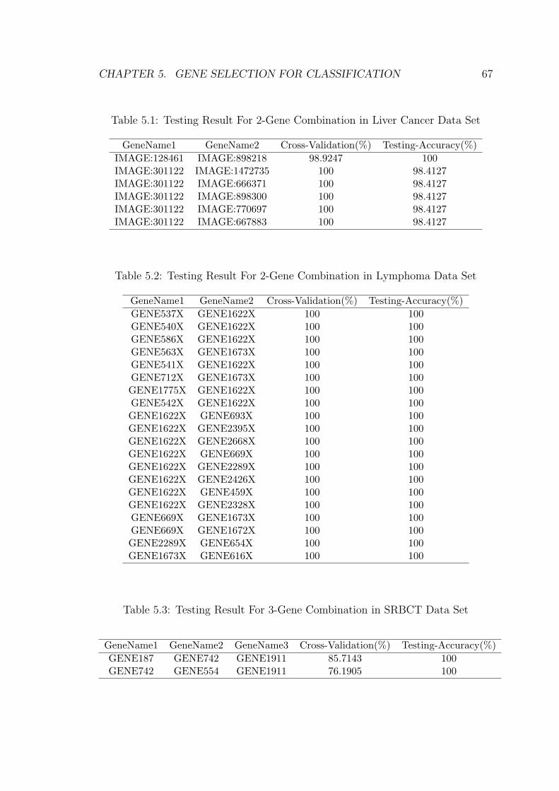
CHAPTER 5. GENE SELECTION FOR CLASSIFICATION 67
Table 5.1: Testing Result For 2-Gene Combination in Liver Cancer Data Set
GeneName1 GeneName2 Cross-Validation(%) Testing-Accuracy(%)IMAGE:128461 IMAGE:898218 98.9247 100IMAGE:301122 IMAGE:1472735 100 98.4127IMAGE:301122 IMAGE:666371 100 98.4127IMAGE:301122 IMAGE:898300 100 98.4127IMAGE:301122 IMAGE:770697 100 98.4127IMAGE:301122 IMAGE:667883 100 98.4127
Table 5.2: Testing Result For 2-Gene Combination in Lymphoma Data Set
GeneName1 GeneName2 Cross-Validation(%) Testing-Accuracy(%)GENE537X GENE1622X 100 100GENE540X GENE1622X 100 100GENE586X GENE1622X 100 100GENE563X GENE1673X 100 100GENE541X GENE1622X 100 100GENE712X GENE1673X 100 100GENE1775X GENE1622X 100 100GENE542X GENE1622X 100 100GENE1622X GENE693X 100 100GENE1622X GENE2395X 100 100GENE1622X GENE2668X 100 100GENE1622X GENE669X 100 100GENE1622X GENE2289X 100 100GENE1622X GENE2426X 100 100GENE1622X GENE459X 100 100GENE1622X GENE2328X 100 100GENE669X GENE1673X 100 100GENE669X GENE1672X 100 100GENE2289X GENE654X 100 100GENE1673X GENE616X 100 100
Table 5.3: Testing Result For 3-Gene Combination in SRBCT Data Set
GeneName1 GeneName2 GeneName3 Cross-Validation(%) Testing-Accuracy(%)GENE187 GENE742 GENE1911 85.7143 100GENE742 GENE554 GENE1911 76.1905 100
CHAPTER 5. GENE SELECTION FOR CLASSIFICATION 68
Figure 5.2: Top 196 Genes of Lymphoma Data Set According to T-Score
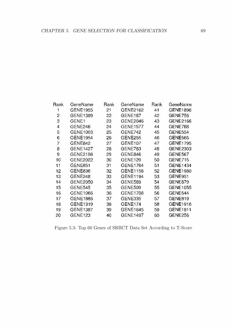
CHAPTER 5. GENE SELECTION FOR CLASSIFICATION 69
Figure 5.3: Top 60 Genes of SRBCT Data Set According to T-Score
Chapter 6
Conclusion and Future Works
6.1 Conclusion
In our biclustering study, we have re-looked at the problem of discovering biclusters
in microarray gene expression data set. We propose a generalization of a framework
for biclustering. From this base,we have proposed a new approach that exploits
frequent pattern mining to deterministically generate an initial set of good quality
biclusters. The biclusters generated are then further refined by adding more rows
and/or columns to extend their volume while keeping their mean squared residue
below a certain predetermined threshold. We have implemented our algorithm,
and tested it on the Yeast data set and human Lymphoma data set. The results of
our study showed that our algorithm, DBF, can produce better quality biclusters
than FLOC in comparable running time. Our frame work does not only concisely
generalize the recently research on biclustering, but also give us a clear path in this
area
In our work of gene selection, we propose a very simple yet very effective method
to find minimal and optimal subset of genes. We applied our method to three well-
known microarray data sets, i.e., liver cancer data set, lymphoma data set, and the
70
CHAPTER 6. CONCLUSION AND FUTURE WORKS 71
SRBCT data set. The results in all the data sets indicate that our method can find
minimum gene subsets that can ensure very prediction accuracy. The significance
of finding this minimum gene subsets is three-fold:
1. It greatly reduces the computational burden and ”noise” arising from irrele-
vant genes.
2. It simplifies gene expression tests to include only a very small number of
genes rather than thousands of genes.
3. It calls for further investigations into possible biological relationship between
these small number of genes and cancer development and treatment.
In addition, although the t-test [DP97] based approach have been proven to
be effective in selecting important genes for reliable prediction, it is not a perfect
tool. To find minimum gene subsets that ensure accurate predictions, we must also
consider the cooperations between genes.
6.2 Future Work
In the future research in biclustering, we should do more studies on improve fre-
quent pattern mining algorithm to let it be more suitable for gene expression data
so that we can accurately find biclusters in a data set without second phase in the
frame work. Since at the moment, frequent pattern mining only can approximate
a bicluster and we need second phase to refine the bilcusters found by it. In the
future study, we can do more research on modifying or propose a new way to find
biclusters using frequent pattern mining alone.
In the future for gene selection in classification, we will do more studies on more
efficient algorithm on gene selection when the number of minimum optimal subset

CHAPTER 6. CONCLUSION AND FUTURE WORKS 72
of genes exceed 4, 5, 6 and so on. Meanwhile the number of top genes selected
from the t-test list is by experience, more research should be done on what is the
effective number of top genes that we should dig in to find the optimal subsets.
Bibliography
[Aas01] Kjersti Aas. Microarray data mining:a survey. http :
//www2.nr.no/documents/samba/researchareas/SIP/microarraysurvey.pdf ,
2001.
[AED+00] A.A. Alizadeh, M.B. Eisen, R.E. Davis, C.Ma, I.S. Lossos, A. Rosen-
wald, J.C. Blodrick, H. Sabet, T. Tran, X. Yu, J. I. Powell, L. Yang,
G. E. Marti, T. Moore, J. H. Jr, L. Lu, D. B. Lewis, R. Tibshirani,
G. Sherlock, W. C. Chan, T. C. Greiner, D. D. Weisenburger, J. O.
Armitage, R. Warnke, R. Levy, W. Wilson, M. R. Graver, J. C. Byrd,
D. Botstein, P. O. Brown, and L. M. Staudt. Distinct types of diffuse
large b-cell lymphoma identified by gene expression profiling. Nature,
403:503–511, 2000.
[ARC00] J. Aach, W. Rindone, and G. M. Church. Systematic management
and analysis of yeast gene expression data. Genome Res., 10:431–45,
2000.
[BDCKY02] A. Ben-Dor, B. Chor, R. Karp, and Z. Yakhini. Discovering local
structure in gene expression data: the order-preserving submatrix
problem. In Proceedings of the sixth annual international conference
on Computational biology, pages 49 – 57, Washington, DC, USA, 2002.
73
BIBLIOGRAPHY 74
[BDD+00] C. A. Ball, K. Dolinski, S. S. Dwight, M. A. Harris, L. Issel-Tarver,
A. Kasarskis, C. R. Scafe, G. Sherlock, G. Binkley, H. Jin, M. Kaloper,
S. D. Orr, M. Schroeder, S. Weng, Y. Zhu, D. Botstein, and J. M.
Cherry. Integrating functional genomic information into the saccha-
romyces genome database. Nucleic Acids Res., 28:77–80, 2000.
[CC00] Y. Cheng and G.M. Church. Biclustering of expression data. In Proc
Int Conf Intell Syst Mol Biol. 2000, pages 93–103, 2000.
[CCS+02] X. Chen, S.T. Cheung, S. So, S.T. Fan, C. Barry, J. Higgins, K.M.
Lai, J. Ji, S. Dudoit, and I.O. Ng. Gene expression patterns in human
liver cancers. Molecular biology of the cell, 13:1929–1939, 2002.
[CDB97] Y. Chen, E. Dougherty, and E. M. L. Bittner. Ratio-based decisions
and the quantitative analysis of cdna microarray images. Journal of
Biomedical Optics, 2:346–374, 1997.
[CL02] C.C. Chang and C.J. Lin. A comparison of methods for multi-class
support vector machines. IEEE Transactions on Neural Network,
13:415–425, 2002.
[DFS00] S. Dudoit, J. Fridlyand, and T. Speed. Comparison of discrimination
methods for the classification of tumors usign gene expression data.
Technical report no. 576, Unversity of California, Berkely, August
2000.
[DP97] J. Devore and R. Peck. Statistics: the exploration and analysis of
data. 3rd eidtion. Duxbury Press, Pacific Grove, CA, 1997.
[DPB+96] J. DeRisis, L. Penland, P. O. Brown, M. L. Bittner, P. S. Meltzer,
M. Ray, Y. Chen, Y. Su, and J. M. Trent. Use of a cdna microarray
BIBLIOGRAPHY 75
to analyse gene expression patterns in human cancer. Nat Genet,
14:457–460, 1996.
[GLD00] G.Getz, E. Levine, and E. Domany. Coupled two-way clustering anal-
ysis of gene microarray data. Proc Natl Acad Sci U S A., 97:12079–84.,
2000.
[GST+99] T. R. Golub, D. K. Slonim, P. Tamayo, C. Huard, M. Gaasenbeek,
J.P. Mesirov, H. Coller, M. Loh, J. R. Downing, M. A. Caligiuri, C. D.
Bloomfield, and E. S. Lander. Molecular classification of cancer: class
discovery and class prediction by gene expressin monitoring. Science,
pages 531–537, October 15 1999.
[Har75] J. Hartigan. Clustering Algorithms. John Wiley and Sons, 1975.
[HK01] Jiawei Han and Micheline Kamber. Data mining concepts and tech-
niques. Morgan Kaufmann, San Francisco, CA, USA, 2001.
[KKB03] I. S. Kohane, A. T. Kho, and A. J. Butte. Microarrays for an inte-
grative genomics. MIT Press, London, England, 2003.
[KMC00] M. K. Kerr, M. Martin, and G. A. Churchill. Analysis of variance for
gene expression microarray data. Journal of Computational Biology,
7:819–837, 2000.
[KSHR00] A. D. Keller, M. Schummer, L. Hood, and W. L. Ruzzo. Bayesian
classification of dna array expression data. Technical report UW-CSE-
2000-08-01, Unversity of Washington, August 2000.
[KWR+01] J.M. Khan, J.S. Wei, M. Ringner, L.H. Saal, M. Ladanyi, F. West-
ermann, F. Berthold, M. Schwab, C.R. Antonescu, and C. Peterson.
BIBLIOGRAPHY 76
Classification adn diagnostic prediction of cancers using gene expres-
sion profiling and artificial neural networks. Nature Medicine, 7:673–
679, 2001.
[LO02] Laura Lazzeroni and Art Owen. Plaid models for gene expression
data. Laura Lazzeroni and Art Owen Statistica Sinica, 12:61–86, 2002.
[NKR+01] M. A. Newton, C. M. Kendziorski, C. S. Richmond, F. R. Blattner,
and K. W. Tsui. On differential variability of expression ratios: im-
proving statistical inference about gene expression changes from mi-
croarray data. Journal of Computational Biology, 8:37–52, 2001.
[PPB01] P. J. Park, M. Pagano, and M. Bonetti. Nonparametric scoring al-
gorithm for identifying informative genes from microarray data. In
Pacific Symposium on Biocomputing 2001, January 2001.
[SC00] M. Sapir and G. A. Churchill. Estimating the posterior probability
of differential gene expression from microarray data. Poster, The
Jackson Laboratory, 2000.
[SSH+96] M. Schena, D. Shalon, R. Heller, A. Chai, P. O. Brown, and R. W.
Davis. Parallel human genome analysis: microarray-based expression
monitoring of 1000 genes. Proc. Natl. Acad. Sci., 93:10614–10619,
1996.
[STG+01] E. Segal, B. Taskar, A. Gasch, N. Friedman, and D. Koller. Rich
probabilistic models for gene expression. Bioinformatics, 17:243–52,
2001.
BIBLIOGRAPHY 77
[TCS+01] O. Troyanskaya, M. Cantor, G. Sherlock, P. Brown, T. Hastie, R. Tib-
shirani, D. Botstein, and R. B. Altman. Missing value estimation
methods for DNA microarrays. Bioinformatics, 17:520–525, 2001.
[THC+99] S. Tavazoie, J.D. Hughes, M. J. Campbell, R. J. Cho, and G. M.
Church. Systematic determination of genetic network architecture.
Nat Genet, 22:281–5, 1999.
[THNC03] R. Tibshirani, T. Hastie, B. Narasimhan, and G. Chu. Class predic-
tion by nearest shrunken centroids with application to dna microarray.
Statistical Science, 18:104–117, 2003.
[TSS02] Amos Tanay, Roded Sharan, and Ron Shamir. Discovering statisti-
cally significant biclusters in gene expression data. Bioinformatics.
Oxford University Press, 18:136–144, 2002.
[TTC98] V. G. Tusher, R. Tibshirani, and G. Chu. Significance analysis of
microarrays applied to the ionizing radiation response. In Proc. Natl.
Acad. Sci. USA 98, pages 5116–5121, 1998.
[WWYY02] Haixun Wang, Wei Wang, Jiong Yang, and Philip S. Yu. Clustering
by pattern similarity in large data sets. In SIGMOD’2002, pages
126–133, Madison, Wisconsin, USA, June 2002.
[YWWY03] Jiong Yang, Haixun Wang, Wei Wang, and Philip S. Yu. Enhanced
biclustering on expression data. In BIBE 2003, pages 321–327, March
2003.
[YYYZ03] X. Yu, L. Yuan, X. Yuan, and F. Zen. Basics of molecular biology.
http://www.comp.nus.edu.sg/ ksung/cs5238/2002Sem1/note/lecture1.pdf,
Lecture Note for CS5238, NUS, Singapore, 2003.

BIBLIOGRAPHY 78
[ZH02] M. J. Zaki and C. Hsiao. Charm: An efficient algorithm for closed
itemset mining. In 2nd SIAM International Conference on Data Min-
ing, Arlington,USA, April 2002.