GENE EXPRESSION AND MULTIPLE REGRESSION MODELS …iwtc.info/wp-content/uploads/2013/11/238.pdf · GENE EXPRESSION AND MULTIPLE REGRESSION MODELS ... Essam A. Gooda 1 and Mohamed A

Seventeenth International Water Technology Conference, IWTC17 Istanbul, 5-7 November 2013

GENE EXPRESSION AND MULTIPLE REGRESSION MODELS

FOR THE COST OF BRIDGE AND CULVERT

Essam A. Gooda 1 and Mohamed A. Nassar

2

1 Professor of Water resources Engineering, Civil Engineering Dept. Beirut Arab University, Debiah, Lebanon.

[email protected] 2 Associate professor, Water and Water Structures Eng. Dept., Faculty of Eng., Zagazig University, Zagazig,

[email protected]

ABSTRACT

The present paper is directed to the trouble of the cost comparison between the culvert and

the bridge. In addition, a combined effort of cost analysis and modeling approach is

presented. The predictions of the cost for both culvert and bridge are presented using Gene

Expression Programming (GEP) and Multiple Linear Regression (MLR). Furthermore, The

predictions of the cost using (GEP) and (MLR) are compared. The concept of using reference

bridge and reference culvert is introduced. GEP approach is able to manage effectively with

data gaps. Statistics and scatter plots indicate that the new approach produces acceptably

results and can be used as an alternative to the MLR. GEP models predict the cost ratio for all

datasets with a relatively higher accuracy (R2 is 3.0% more than MLR), higher correlation

(1% more than MLR), and lower error RMSE (0.007% less than MLR).

Keywords: bridge, culvert, Gene Expression Programming and cost analysis.

1. INTRODUCTION

Prediction of hydraulic variables are extremely required in the design process.

Because of difficulty of many phenomena, more strong tools are required for model purposes.

When a road crosses a canal or drain, either a bridge or culvert may be a good solution.

However, a civil engineer is always seeking for a decision; which one is more economic?.

The decision is not an easy task. It depends on several criteria. The factors affecting the

choice are many. Yassin (1988), presented a procedure for the economic sizing of box

culverts. He formulated a set of 13 accurate dimensionless equations for the estimation of the

cost of 13 different box culvert sizes. Bridge was not included in the paper. Mostafa Gooda,

(2003), presented two statistical equations to simulate the cost of bridge and culvert. The A

review for the comparison between the cost of both the bridge an culvert were presented by

Mostafa Gooda, (2003).


Many of the studies were presented to compare between bridge and culver

depending on the multiple linear regression techniques (MLR). Fortunately, relatively new

and efficient computational techniques were developed and being applied in most of

engineering application. One of these promising techniques is Gene Expression

Programming (GEP). GEP was successfully applied in maritime engineering by Kalra and

Deo, (2007), Singh et al., (2007), Gaur and Deo, (2008), Ustoorikar and Deo, (2008). The

present paper concentrates on the cost comparison of both culvert and bridge. In addition, it

aims to model the cost for both structures using Gene Expression Programming (GEP) and

compare the results with the multiple regression techniques (MLR). The performance of the

present equations are compared to actual cost values. The results allow for the designer

engineer to decide which one is more economic, the culvert or the bridge.

2. DESIGN GUIDELINES AND ASSUMPTIONS FOR THE BRIDGE AND

CULVERT

The design guidelines have been developed by Mostafa, (2003). The general layouts of a

sample of both bridge and culvert are shown in Figs. (1 and 2), respectively. For bridge, the

components includes the superstructure (slab, cross girders, and main girders), substructure

and wing walls. On the other hand, the culvert’s components include the box culvert vent

and wing walls. The following assumptions are considered:

The wing walls are of box type for both bridge and culvert;

The bearing capacity of soil is: = 1.0 kg/cm2;

For culvert, only one vent box type is considered;

The live load considered in design of bridge is 60 ton lorry and a surcharge of

600kg/m2

is considered in the design of different components of both structures;

The data of soil properties are: soil =1.8 t/m3 and =30

o;

The compressive strength of reinforced concrete is, fcu=325 Kg/cm2 and the strength

of high tensile steel is; fs = 1600 Kg/cm2;

The Quantity of Portland cement is 400 Kg/m3; and

The price list for bridge and culvert components is given in table (1).

Table (1) The prices list for the different components of bridge and culvert according

to Egyptian market price of 2010 [Mostafa Gooda, E.A., 2003]

Bridge Culvert

Component Price ($/m3)×1000 Component Price ($/m

3) )×1000

RC superstructure 326.31 RC walls 252.63

RC walls 252.63 RC floor 200.00


RC floor 200.00 PC floor 97.36

PC floor 97.36

3. DIMENSIONLESS PARAMETERS

The cost of the different structures’ components according to Egyptian market’ prices

depends on many variables. For purpose of presenting the non-dimensional relationships, a

concept of reference bridge as well as reference culvert is introduced. Both the reference

bridge and the reference culvert are selected from Table (2) so that their costs are identical.

These variables can be grouped for bridge and culvert cases as following:

Fig. 1 Schematic schetches for an example of the bridge

0,,,,,,,,, Wbrbrbrbrb LWSHWSHCCf ….……..……………………………....…..…(1)

0,,,,,,,,,,, Wcvcvcvrcvrcrcrcrc LHLWHHLWHCCf …….……………….……...……...(2)


in which: Cb is the bridge cost in (US Dollars); Cbr is the cost of the reference bridge =

49.6×103 $; Hbr is the height between road level and bed level of canal or drain for reference

bridge case= 4.0 m; Sbr is the bridge span for reference bridge case = 6.0 m; Wbr is the road

width for reference bridge case = 6.0 m; H is the height between road level and bed level of

canal or drain; S is the bridge span; W is the road width;

site; LW is the length of wing walls; Cc is the culvert cost in (US Dollars); Ccr is the cost of

the reference culvert = 49.6×103 $; Hcr is the height between road level and bed level of canal

or drain for reference culvert case = 4.0 m; Wcr is the road width for reference culvert case =

6.0 m; Lcvr is the width of clear vent for reference culvert case = 2.0 m; Hcvr is the height of

clear vent for reference culvert case = 2.0 m; Lcv is the width of clear vent; and Hcv is the

height of clear vent. The dimensionless relationships of the bridge and culvert costs and

other independent parameters could be determined relative to the characteristics of the

reference unites as following:

bratiobratiobratiobratio WSHfC ,, ….…………………………………...………….….…...…(3)

cvratiocvratiocratiocratiocratio HLWHfC ,,, …….……………......................................…..…...(4)

In which: Cbratio= Cb/Cbr is the relative bridge cost; Hbratio= H/Hbr is the relative

height between road level and bed level of canal or drain; Sbratio= S/Sbr is the relative bridge

span; Wbratio= W/Wbr is the relative road width; Ccratio= Cc/Ccr is the relative culvert cost;

Hcratio= H/Hcr is the relative height between road level and bed level of canal or drain;

Wcratio= W/Wcr is the relative road width; Lcvratio= Lcv/Lcvr is the relative width of clear vent;

Hcvratio = Hcv/Hcvr is the relative height of clear vent.

4. PROPOSED DESIGN SOFTWARE

Two different computer programs are designed, well verified and calibrated to perform

several procedures for the design of different components of both bridge and culvert,

Mostafa, E.A. 2003. The outputs of the programs give:

Straining actions;

Stress distribution;

Stability calculation against sliding and overturning;

Complete structural design for different components; and

Cost of the unit. (i.e., the bridge or culvert)

For bridges, several values of H, the difference between the road level and bed levels,

are considered. These values are, H = 4, 4.5, 5, 5.5, 6, 6.5 m. For each value of H, all bridge


components are estimated and consequently, the cost is determined based on the price list

shown in Table (1). Also, different road widths, W = 6, 8, 10 m, and different span values, S

= 6, 8, 10 m, are considered. On the other hand for culverts, same height values; H = 4, 4.5,

5, 5.5, 6, 6.5 m and same road widths, W = 6, 8, 10 m are considered. Moreover, several

dimensions of the clear vent width, Lcv , and the height of clear vent, Hcv are used, (i.e., Lcv

=3; and 2; Hcv =3; and 2). Characteristics of bridges and culverts as well as their estimated

costs are summarized for 15-selected cases in Table (2). Costs of 54 different bridges and

costs of 72 different culverts are used in this paper.


Fig. 2 Schematic schetches for an example of the culvert

Table (2) Selected estimated cost of the bridges and culvers [Mostafa, E.A., 2003]

Series Wbratio Sbratio Hbratio Cbratio Wcratio Hcratio Lcvratio Hcvratio Ccratio

1 1.00 1.67 1.63 2.75 1.00 1.63 1.00 1.00 1.12

2 1.33 1.67 1.63 3.13 1.00 1.50 1.00 1.00 1.09

3 1.67 1.67 1.63 3.49 1.00 1.38 1.00 1.00 1.07

4 1.33 1.67 1.50 2.81 1.33 1.13 1.00 1.00 1.06


5 1.33 1.00 1.50 2.33 1.67 1.13 1.00 1.00 1.10

5. MULTIPLE LINEAR REGRESSION (MLR)

Based on the design data, several statistical equations were used to predict the relative

bridge cost; Cbratio and the relative culvert cost; Ccratio. The following equations represent non-

dimensional form of the bridge and culvert cost ratio; respectively.

472.0354.0793.1

bratiobratiobratiobratio WSHC ….…………………………………….…..…...…(5)

256.0180.0201.0289.0

cvratiocvratiocratiocratiocratio HLWHC …….……………........……...……...(6)

Equation (5) represents a non-dimensional form can be applied to estimate the cost

ratio of an existing bridge relative to that of the reference bridge. On the other hand, equation

(6) represents a non-dimensional form can be applied to estimate the cost ratio of an existing

culvert relative to that of the reference culvert. The objective function (i.e., the function is

used to measure the accuracy of the MLR equations) values are calculated from the

proportion of variance, which is the best single measure of how well the predicted values

match the actual values. This is also known as the "coefficient of determination RSQ or R2"

as presented in Eq. (7). In addition, the correlation factor is used as a second measure factor.

The quantity r, called the linear correlation coefficient, measures the strength and the

direction of a linear relationship between two variables. The mathematical formula for

computing r can be presented as shown in Eq. (8). The last measure to the accuracy of the

equations (5) and (6) is the Root Mean Square Error (i.e., RMSE). It can be calculated as

presented in Eq. (9).

)X(X))X(Y Rj

i

j

i

222 …….……………...............................................…..…...(7)

5.02222 )))()()((()()( YYNXXNYXXYNrnCorrelatio …………...(8)

NXYRMSEj

i

2)( …….……………...................................................................…..…...(9)

where Y is the predicted variable, X is the measured variable, X

is the sample mean of X

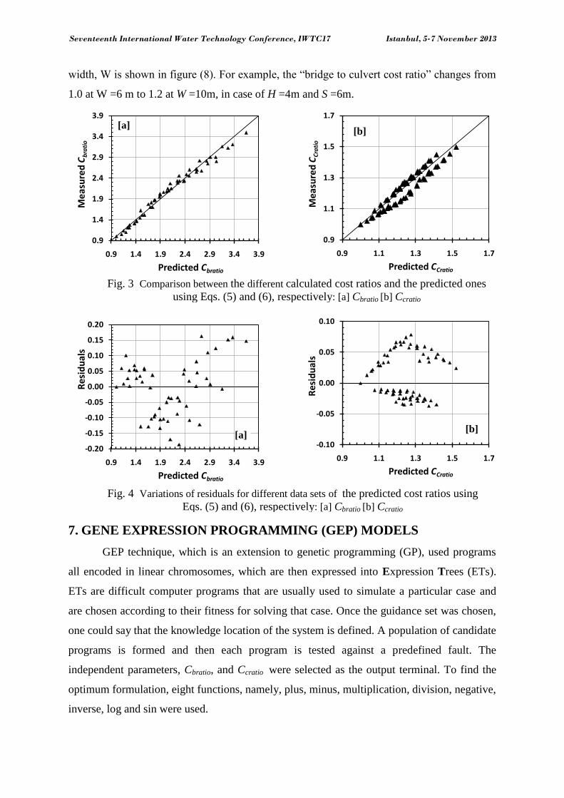
value and N the total number of variables. Figures (3A and 3B) show a comparison between

the calculated Cbratio and Ccratio and the predicted values using Eqs. (5) and (6), respectively.

A good agreement can be noticed, to some extent. The residuals of the previous equations are

plotted versus the predicted values as shown in (3a and 3b). The residuals show random

distribution around the line of zero in case of equation (5), while it follows a specified trend

http://en.wikipedia.org/wiki/Random_variables

http://en.wikipedia.org/wiki/Random_variables

http://en.wikipedia.org/wiki/Arithmetic_mean


for equation (6). The regression statistics have been listed in the table (3). Results of MLR

emphasis the nead to adopt a new technique like Gene Expression Programming (GEP).

Table (3) Basic Features of the developed MLR models equations (5) and (6).

MLR Models R2

RMSE Correlation factor

Equation (5) 0.941 0.092 0.990

Equation (6) 0.878 0.034 0.938

Dividing equation (5) by equation (6) gives the following equation:

2560.01801.02013.02893.0

472.0354.0793.1

cvratiocvratiocratiocratio

bratiobratiobratio

cratio

bratio

HLWH

WSH

C

C

….………..…..…....…….…….(7)

As mentioned before, the costs of both reference bridge and reference culvert are the

same. Therefore: cbcratiobratio CCCC . This means that:

2560.01801.02013.02893.0

472.0354.0793.1

cvratiocvratiocratiocratio

bratiobratiobratio

c

b

HLWH

WSH

C

C

….……………..…..…..…..……...(8)

For the same road width, and the same height between road level and bed level of

canal or drain, in both bridge and culvert, equation (8) may take the following form:

2560.01801.0

354.0270.0503.1

cvratiocvratio

bratio

c

b

HL

SWH

C

C

….……………..…..…..…..…....………..…..….....……...(9)

In which: Cb is the bridge cost in (US Dollars); Cc is the culvert cost in (US Dollars);

H is the height between road level and bed level of canal or drain; and W is the road width;

Sbratio is the relative bridge span; Lcratio is the relative width of the culvert clear vent; Hcratio is

the relative height of the culvert clear vent..

6. ANALYSIS OF THE OUTPUTS USING THE MULTIPLE LINEAR

REGRESSION (MLR)

The effect of the height between road level and bed level of canal or drain on the cost

for both bridge and culvert is shown Figs. (5, 6 and 7) for W = 6, 8, 10 m, respectively. For

bridge, the rate of change is steeper than that for culvert. The trend is logic where increasing

the value of H or bridge height, leads to increase height and thickness of not only abutment

but also wing walls. For culvert, H is just a fill height above culvert. In contrast, it can be

noticed that there is a short range for H at which the cost of the bridge may be more

economic in comparison with the culvert cost. The results of regression analysis show that for

bridge, the power, of H is 1.793 while it is 0.289 in case of culvert. The effect of road


width, W is shown in figure (8). For example, the “bridge to culvert cost ratio” changes from

1.0 at W =6 m to 1.2 at W =10m, in case of H =4m and S =6m.

7. GENE EXPRESSION PROGRAMMING (GEP) MODELS

GEP technique, which is an extension to genetic programming (GP), used programs

all encoded in linear chromosomes, which are then expressed into Expression Trees (ETs).

ETs are difficult computer programs that are usually used to simulate a particular case and

are chosen according to their fitness for solving that case. Once the guidance set was chosen,

one could say that the knowledge location of the system is defined. A population of candidate

programs is formed and then each program is tested against a predefined fault. The

independent parameters, Cbratio, and Ccratio were selected as the output terminal. To find the

optimum formulation, eight functions, namely, plus, minus, multiplication, division, negative,

inverse, log and sin were used.

0.9

1.1

1.3

1.5

1.7

0.9 1.1 1.3 1.5 1.7

Me

asu

red

CCratio

Predicted CCratio

-0.10

-0.05

0.00

0.05

0.10

0.9 1.1 1.3 1.5 1.7

Re

sid

ua

ls

Predicted CCratio

0.9

1.4

1.9

2.4

2.9

3.4

3.9

0.9 1.4 1.9 2.4 2.9 3.4 3.9

Me

asu

red

Cbratio

Predicted Cbratio

-0.20

-0.15

-0.10

-0.05

0.00

0.05

0.10

0.15

0.20

0.9 1.4 1.9 2.4 2.9 3.4 3.9

Res

idu

als

Predicted Cbratio

Fig. 3 Comparison between the different calculated cost ratios and the predicted ones

using Eqs. (5) and (6), respectively: [a] Cbratio [b] Ccratio

[a] [b]

[a] [b]

Fig. 4 Variations of residuals for different data sets of the predicted cost ratios using

Eqs. (5) and (6), respectively: [a] Cbratio [b] Ccratio

10

Fig. 5 The effect of H on the cost for both

bridge and culvert for W=6m





Fig. 8 The effect of W on the bridge to

culvert cost ratio for S=6m and different H

A large number of generations were needed to find a principle with a minimal fault.

First, the some constants were assigned. With these constants, a large number of generations

were required to reduce the fault. These constants were changed and the program was

executed to search for a principle or formula with minimal fault and as short as possible in

length. The optimum GEP structure had the following characteristics.

[1] The selection is done by taken a random number of individuals from the

population and the best fit is chosen; [2] The operations that were used in this study were

crossover and mutation. They were selected by adopting a rule with a minimum probability

of 0.1; [3] The sum of absolute differences between the obtained and expected values for all

sets of data in the database was used as a measure for fitness; [4] Population size: 50

members; [5] Maximum Gene head length 8.0, [6] gene per chromosome 4.0 and, [6] Total

0.5

1.0

1.5

2.0

2.5

3.0

0.5

1.0

1.5

2.0

2.5

3.0

0.9 1 1.1 1.2 1.3 1.4 1.5 1.6 1.7

Cost/4

9.6

×1

03

($)

H/4 (m)W=6.0m & S=6.0m

W=6.0m & Lcv=2.0m & Hcv=2.0m

W=6.0m & Lcv=2.0m & Hcv=3.0m

0.5

1.0

1.5

2.0

2.5

3.0

0.5

1.0

1.5

2.0

2.5

3.0

0.9 1 1.1 1.2 1.3 1.4 1.5 1.6 1.7

Cost/4

9.6

×1

03

($)

H/4 (m)W=8.0m & S=6.0m W=8.0m & Lcv=2.0m & Hcv=2.0mW=8.0m & Lcv=2.0m & Hcv=3.0m

0.50

1.00

1.50

2.00

2.50

3.00

0.5

1.0

1.5

2.0

2.5

3.0

0.9 1 1.1 1.2 1.3 1.4 1.5 1.6 1.7

Cost/4

9.6

×1

03

($)

H/4 (m)

W=10.0m & S=6.0m

W=10.0m & Lcv=2.0m & Hcv=2.0m

W=10.0m & Lcv=2.0m & Hcv=3.0m

0.5

1.0

1.5

2.0

2.5

3.0

0.9 1 1.1 1.2 1.3 1.4 1.5 1.6 1.7

Cb/C

c

W/6 (m)H=4 & S=6m H=4.5 & S=6mH=5.5 & S=6m H=6 & S=6mH=6.5 & S=6m

11

generations are 2000. After incorporating the corresponding values and making necessary

simplifications, the final equations become:

bratiobratiobratiobratio

bratio

bratiobratiobratio HSWH

W

SWC

sin …………………………….……………..(10)

25.025.0 )())log(( cratiocvratiocratiocvratiocratio HHWLC .........................................................…...(11)

With the all data sets used in this study, approximately 100 percent of these patterns

chosen till the best training performance were seen. Table 4, presents the compiled

measurements. They are graphically shown in Fig. (9) which shows the ordinates of the

calculated independent parameters against the predicted ones. Presence of a small scatter

between these variables can be noted. The statistic measures for both equations (10 and 11)

have been listed in the table (4).

Table (4) Basic Features of the developed GEP models of equations (10 and 11)

GEP Models R2

RMSE Correlation factor

Equation (10) 0.967 0.012 0.992

Equation (11) 0.885 0.033 0.944

8. ANALYSIS OF RESULTS

The independent parameters predictions in the present study has been made on the

basis of outputs data made earlier in Mostafa, E.A. 2003. The Genetic Expression

Programming (GEP), and Multiple Linear Regression (MLR) models, therefore, developed

with the former sets of values as inputs (variables namely, bratiobratiobratio WSH ,, in order to

predict bratioC and cratioC , the cost ratio for both bridge and culvert, respectively.

The statistical results of models predictions for data sets are given in Tables ( 3, and

4). The results of the developed GEP prediction models were compared with the regression

equation formulae (5 6). It was found that the Genetic Expression Programming (GEP)

models are highly satisfactory as seen in Figs. (11, 12,13,14,15 and 16). From the comparison

of the different predictions models, it is clear that GEP models predicted the cost ratio for all

datasets with a relatively higher accuracy (R2 is 3.0% more than MLR), higher correlation

(1% more than MLR), and lower error RMSE (0.007% less than MLR). The acceptable

results of GEP are achieved for simulating the other studied parameters compared to the

MLR models. Further, the scatter plot Fig. (10) proves out the good performing of the GEP.

12

9. APPLIED EXAMPLES

9.1. Example 1

At certain location, estimate the cost of construction for a bridge has the following

characteristics using MLR equation (5) and GEP equation (10):

Road width, W=10 m,

Span, S =10 m, and

Road height above bed , H =6 m

9.2. Solution

The first step is to estimate the relative values:

o bratioW =10/6=1.67, bratioS =10/6=1.67, and bratioH =6/4=1.5

Applying MLR equation (5) to estimate the relative cost of bridge

0.9

1.1

1.3

1.5

1.7

0.9 1.1 1.3 1.5 1.7

Cal

cula

ted

Ccr

atio

Predicted Ccratio

-0.2

-0.1

0.0

0.1

0.2

0.95 1.15 1.35 1.55

Res

idu

als

Predicted Ccratio

0.8

1.6

2.4

3.2

4.0

0.8 1.6 2.4 3.2 4.0

Ca

lcu

late

d C

bra

tio

Predicted Cbratio

-0.4

-0.2

0.0

0.2

0.4

0.8 1.6 2.4 3.2 4.0

Re

sid

ua

ls

Predicted Cbratio

Fig. 9 Comparison between the different calculated cost ratios and the predicted ones

using Eqs. (10 and 11), respectively: [A] Cbratio [B] Ccratio

Fig. 10 Variations of residuals for different data sets of the predicted cost ratios using

Eqs. (10 and 11), respectively: [A] Cbratio [B] Ccratio

[a] [b]

[a] [b]

1

Fig. 11 Comparison between GEP Eq. 11 and

MLR Eq. 6 for the correlation coefficient

Fig. 12 Comparison between GEP Eq. 10 and

MLR Eq. 5 for the correlation coefficient

Fig. 13 Comparison between GEP Eq. 11

and MLR Eq. 6 for R2


and MLR Eq. 5 for R2


and MLR Eq. 6 for RMSE


and MLR Eq. 5 for RMSE

o 472.0354.0793.1

bratiobratiobratiobratio WSHC = (1.5) 1.793

×(1.67)0.354

× (1.67)

0.472

bratioC 3.157

o From the actual data this value is =300.29/94.95 = 3.16

Applying GEP equation (10) to estimate the relative cost of bridge

o )5.167.1()67.1sin(5.167.1

67.167.1

bratioC

o bratioC 3.97

These values mean that the existing bridge costs equal 3.157 and 3.97 times that of

the reference bridge using MLR equation (5) and GEP equation (10), respectively . It

is known that, bratioC Cb/Cbr

0.944

0.938

0.934

0.936

0.938

0.940

0.942

0.944

0.946

Equation (11) Equation (6)

Co

rre

lati

on

0.992

0.99

0.9890

0.9895

0.9900

0.9905

0.9910

0.9915

0.9920

0.9925


Co

rre

lati

on

0.885

0.878

0.876

0.878

0.880

0.882

0.884

0.886


R2

0.967

0.941

0.924

0.931

0.938

0.945

0.952

0.959

0.966

0.973


R2

0.033

0.034

0.0324

0.0327

0.0330

0.0333

0.0336

0.0339

0.0342


RM

SE

0.012

0.092

0.000

0.020

0.040

0.060

0.080

0.100


RM

SE

14

Cbr is the cost of the reference bridge = 49.6×103 $;

Then, the bridge cost; Cb = 156.58×103 $ and 196.9×10

3 $ using MLR equation (5)

and GEP equation (10), respectively.

9.3. Example 2

The above data of bridge given in Example 1 is to be compared with a culvert of the

following characteristics:

o Road width, W=10 m,

o Road height, H =6 m,

o Width of internal vent, Lcv =3,

o Height of internal vent, Hcv =3 m,

9.4. Solution

In example 1, the cost of bridge is estimated. The same procedures can be repeated to

estimate the cost of culvert as following;

5.1;67.1;5.1 cvratiocratiocratio LWH and 5.1cvratioH

Applying MLR equation (6) to estimate the relative cost of culvert

o 256.0180.0201.0289.0 5.15.167.15.1 cratioC 487.1

o From the actual data this value is =139.46/959 = 1.45

Applying GEP equation (11) to estimate the relative cost of culvert

o 324.1)5.15.1())67.15.1log(( 25.025.0 cratioC

These values mean that the existing culvert costs equal 1.487 and 1.324times that of

the reference culvert using MLR equation (6) and GEP equation (11), respectively . It

is known that, cratioC Cc/Ccr

Ccr is the cost of the reference bridge = 49.6×103 $;

Then, the bridge cost; Cc = 73.75×103 $ and 65.69×10

3 $ using MLR equation (6) and

GEP equation (11), respectively.

10. CONCLUSION

The present paper is directed to the trouble of the cost comparison between the culvert

and the bridge. The predictions of the cost for both culvert and bridge are modeled using

Multiple Linear Regression (MLR) and Gene Expression Programming (GEP). A non-

dimensional relationships are presented to estimate the different cost ratios for both bridge

15

and culvert. The results of the developed MLR show that the relationships are simple and

easy to predict the effect of secondary factor on the main factor. GEP prediction models are

compared with the regression equation formulae. It was found that the genetic expression

programming models are highly satisfactory. From the comparison of the different

predictions models, it is clear that GEP models predicted the cost ratio for all datasets with a

relatively higher accuracy, higher correlation and lower error RMSE. The acceptable results

of GEP are achieved for simulating the other studied parameters compared to the MLR

models. Two examples are presented to explain the procedures of estimating the cost of either

a bridge or a culvert.

REFERENCES

[1]. “Hydraulic Charts for •the selection of Highway Culverts,” Hydraulic Engineering

Circular No. 5, U.S.A. Fedral Highway Adminstration, Washington, D.C., 1965.

[2]. Capacity Charts for the Hydraulic Design of Highway Culverts Hydraulic Engineering

Circular No. 10, U.S.A. Fedral Highway Administration, Washington, D.C., 1972.

[3]. Carter, R.W., Computations of Peak discharge at Culverts,” U.S. Geological Survey,

Circular 376, 1957.

[4]. Chow, yen Te, open Channel Hydraulics,” McGraw—Hill Book Company, 1959.

[5]. Wright, P.H. and Paquette, R.J., “Highway Engineering,’ John Wiley & Sons, Fourth

Edition, 1979.

[6]. Yassin, A. A., “Economical Design of Box Culverts,” Alexandria Engineering Journal,

Vol. 27 No. 4, pp. 1-20, October 1988.

[7]. Young, G.K., Childrey, M.R. and Trent, R.E., “Optima]. Design For Highway drainage

Culverts” Journal of the Hydraulics Division, ASCE, Vol. 100, No. HY5, 1974.

[8]. Kalra, R., Deo,M.C., 2007. “Genetic Programming to retrieve missing information in

wave records along the west coast of India”. Applied Ocean Research, Vol. 29, No. 3,

pp.99–111.

[9]. Singh, A.K., Deo, M.C., SanilKumar, V., 2007. “Neural network— genetic

programming for sediment transport”. Journal of Maritime Engineering, The Institution

of Civil Engineers, London, Vol. 160, (MA3), pp.113–119.

[10].Gaur, S., Deo, M.C., 2008. “Real time wave forecasting using genetic programming”.

Journal of Ocean Engineering, Vol. 35, pp.1166–1172.

[11].Ustoorikar, K., Deo, M.C., 2008. “Filling up gaps in wave data with genetic”. Journal of

Programming Marine Structures, Vol. 21, pp.177–195.

16

[12].Gooda, E.A., 2003 “Cost Analysis for Bridge and Culvert”, Seventh International

Egyptian Water Technology Conference, CAIRO, EGYPT, JUNE 3-5, 2003.

Documents

GENE EXPRESSION AND MULTIPLE REGRESSION MODELS …iwtc.info/wp-content/uploads/2013/11/238.pdf · GENE EXPRESSION AND MULTIPLE REGRESSION MODELS ... Essam A. Gooda 1 and Mohamed A