Embed Size (px)
DESCRIPTION
Gene Expression and DNA Chips. Based on slides by Ron Shamir. http://www.bio.davidson.edu/courses/genomics/chip/chip.html. Monitoring Gene Expression. Goal : Simultaneous measurement of expression levels of all genes in one experiment. 2 fundamental biological assumptions: - PowerPoint PPT Presentation
Citation preview
1
Gene Expression and DNA Chips
Based on slides by Ron Shamir
http://www.bio.davidson.edu/courses/genomics/chip/chip.html
2
Monitoring Gene Expression
• Goal: Simultaneous measurement of expression levels of all genes in one experiment.
• 2 fundamental biological assumptions:– Transcription level indicates genes’ regulation.– Only genes that contribute to organism fitness
are expressed.
=> Detecting changes in a gene’s expression level provides clues on the function of its product
3
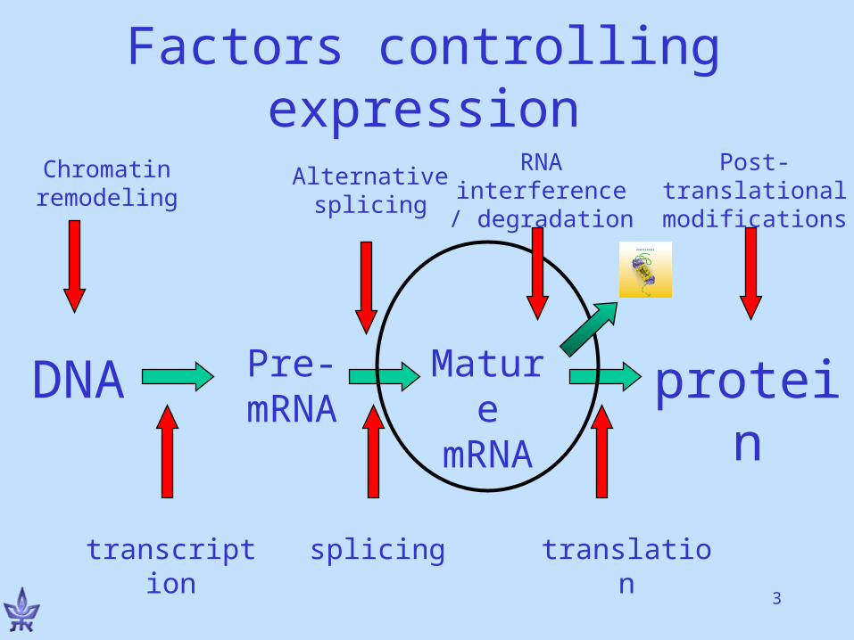
DNA Pre-mRNA
protein
transcription translation
Mature
mRNA
splicing
Factors controlling expression
Post-translational modifications
Chromatin remodeling
Alternative splicing
RNA interference / degradation
4
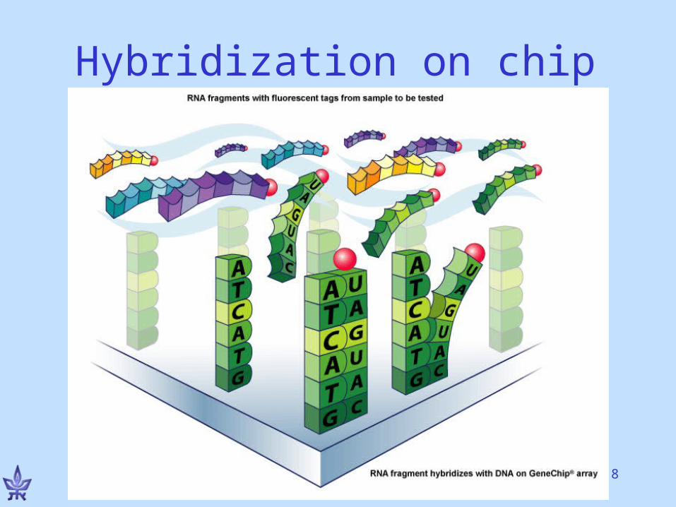
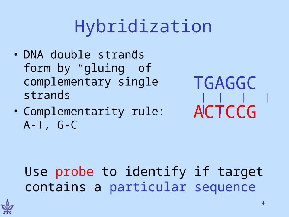
Hybridization• DNA double strands form
by “gluing” of complementary single strands
• Complementarity rule: A-T, G-C
ACTCCG
TGAGGC| | | | | |
Use probe to identify if target contains a particular sequence
5
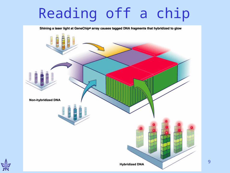
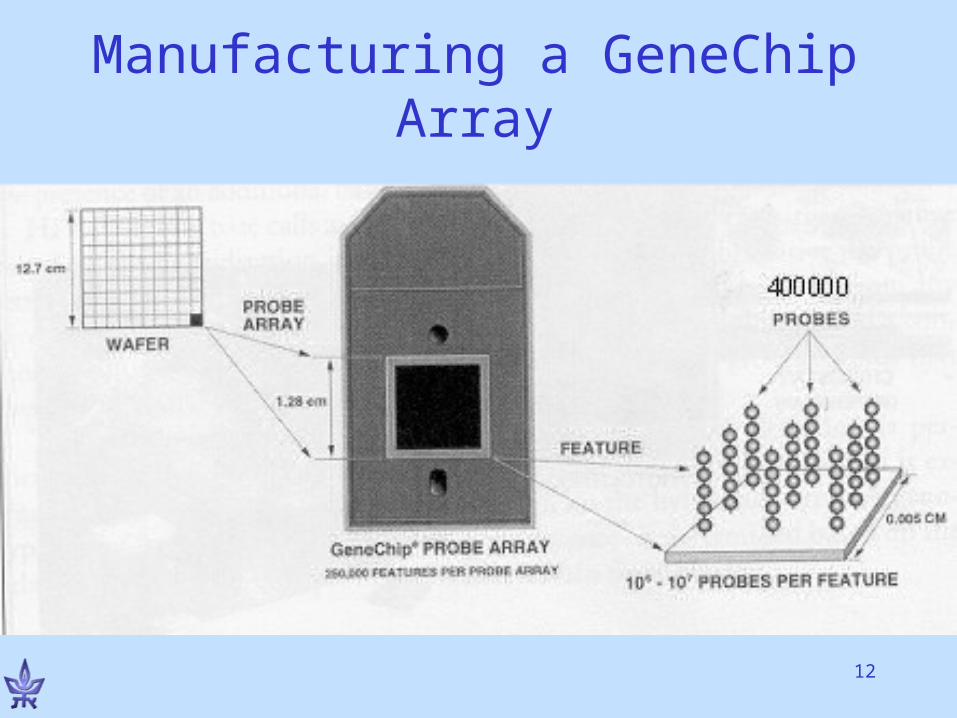
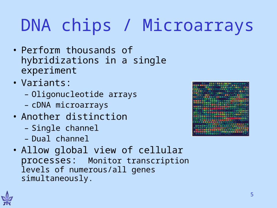
DNA chips / Microarrays• Perform thousands of
hybridizations in a single experiment
• Variants:– Oligonucleotide arrays– cDNA microarrays
• Another distinction– Single channel– Dual channel
• Allow global view of cellular processes: Monitor transcription levels of numerous/all genes simultaneously.
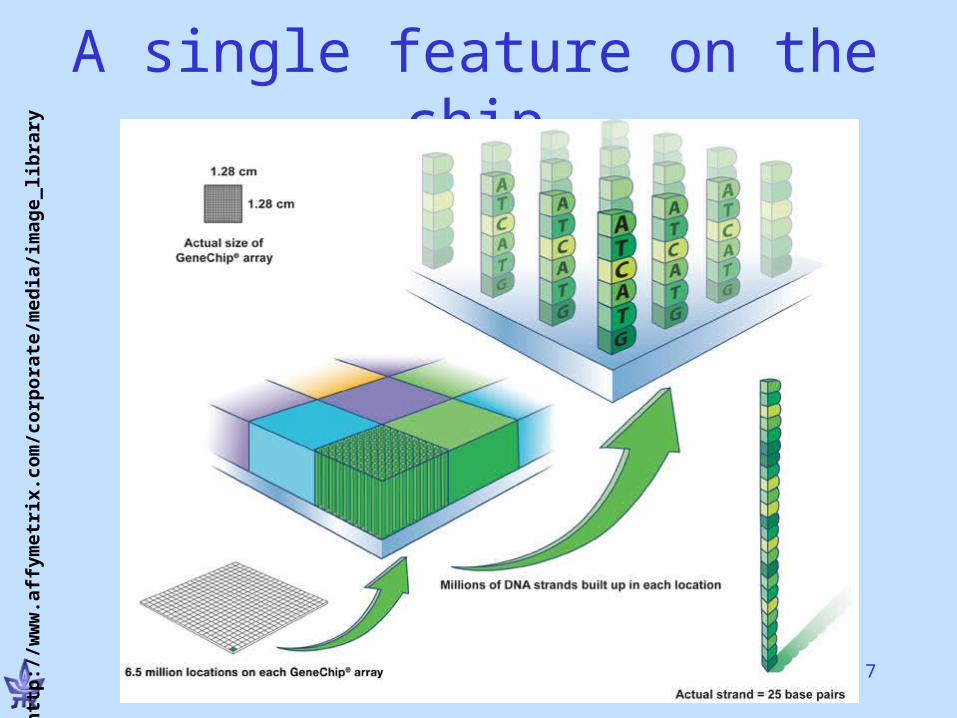
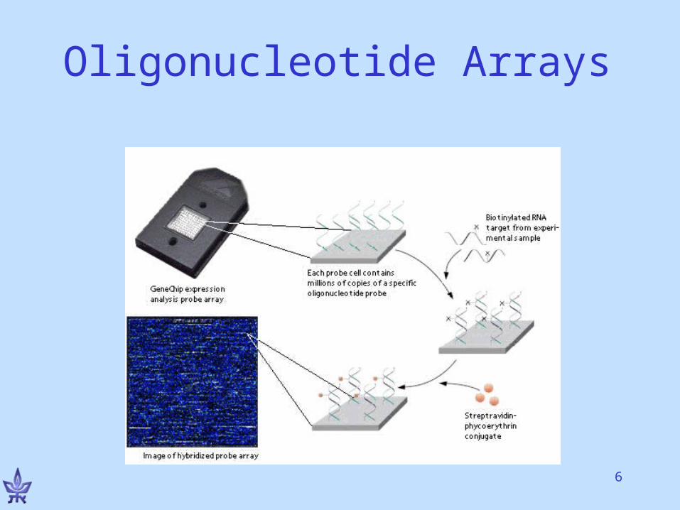
7
A single feature on the chiph
ttp
://w
ww
.aff
ymet
rix.
com
/cor
por
ate/
med
ia/i
mag
e_li
bra
ry/
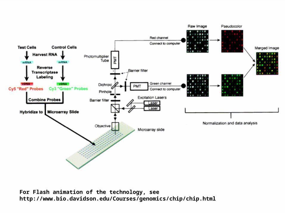
15For Flash animation of the technology, see http://www.bio.davidson.edu/Courses/genomics/chip/chip.html
17
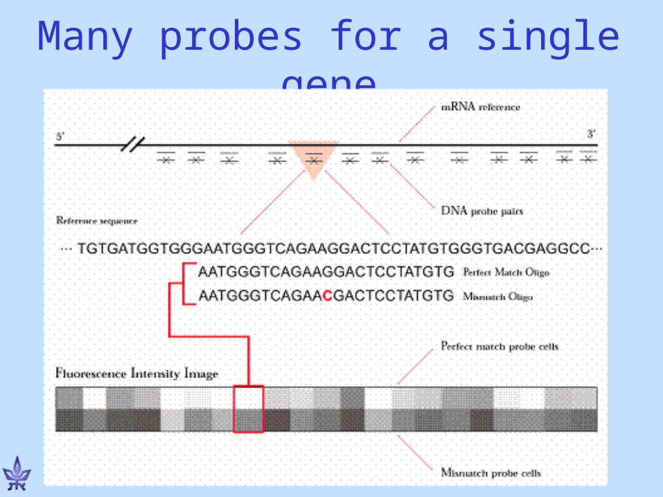
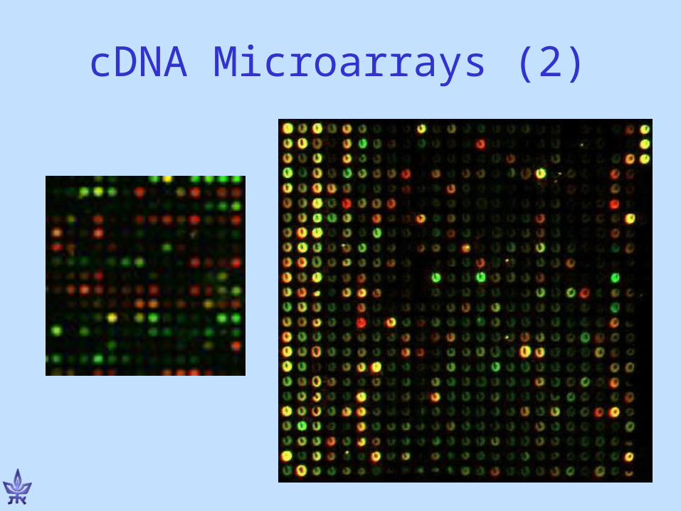
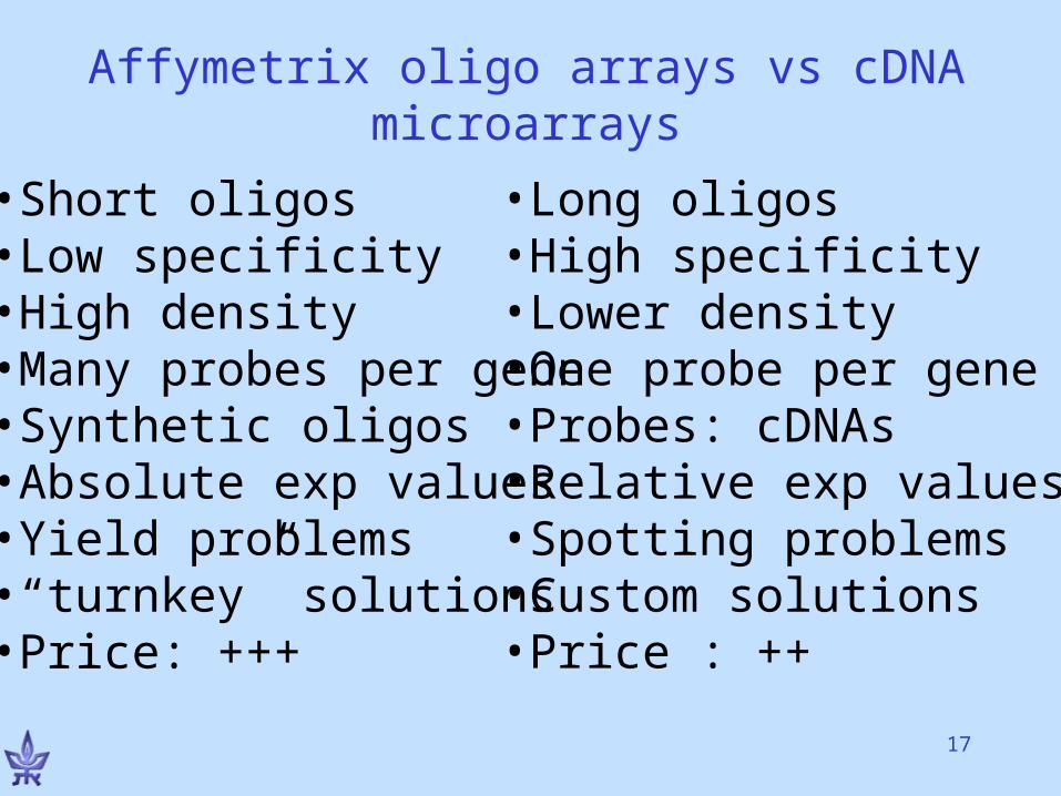
Affymetrix oligo arrays vs cDNA microarrays
•Short oligos•Low specificity•High density•Many probes per gene•Synthetic oligos•Absolute exp values•Yield problems•“turnkey” solutions•Price: +++
•Long oligos•High specificity•Lower density•One probe per gene•Probes: cDNAs•Relative exp values•Spotting problems•Custom solutions•Price : ++
18
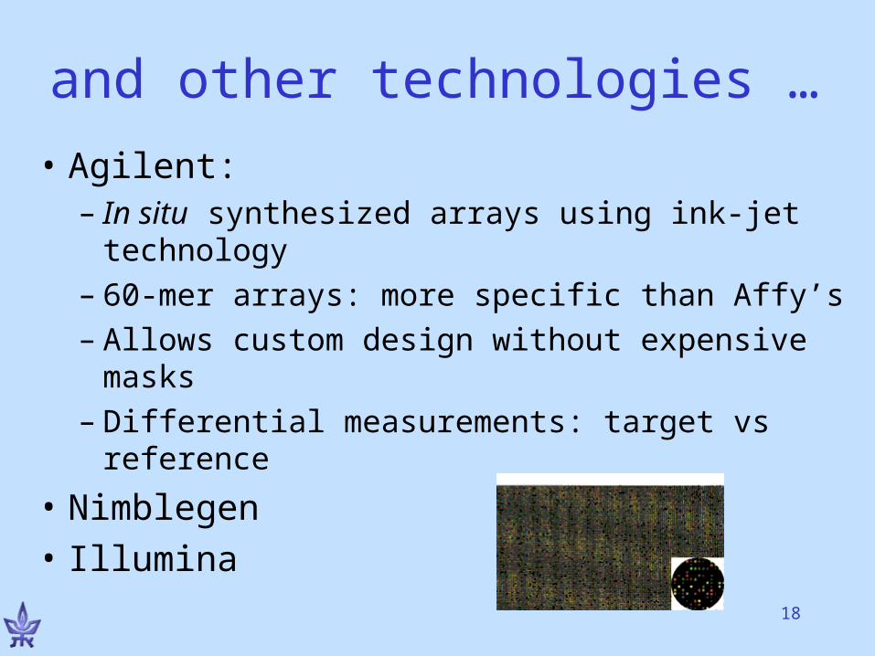
…and other technologies
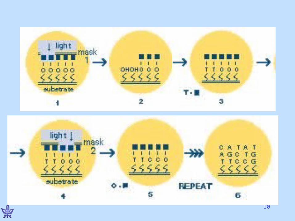
• Agilent:– In situ synthesized arrays using ink-jet
technology– 60-mer arrays: more specific than Affy’s– Allows custom design without expensive
masks– Differential measurements: target vs
reference
• Nimblegen• Illumina

Comparative genomic hybridization (CGH) microarrays
Known DNA sequences
Glass slide
Isolate genomic DNA
Cells of Interest
Reference sample
Flourescently labeled
(almost identical to gene expression arrays, but genomic DNA is hybridized instead of mRNA)
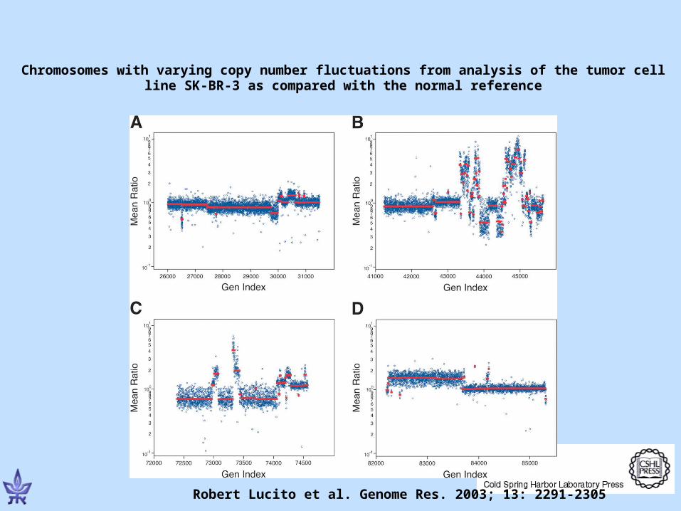
Robert Lucito et al. Genome Res. 2003; 13: 2291-2305
Chromosomes with varying copy number fluctuations from analysis of the tumor cell line SK-BR-3 as compared with the normal reference
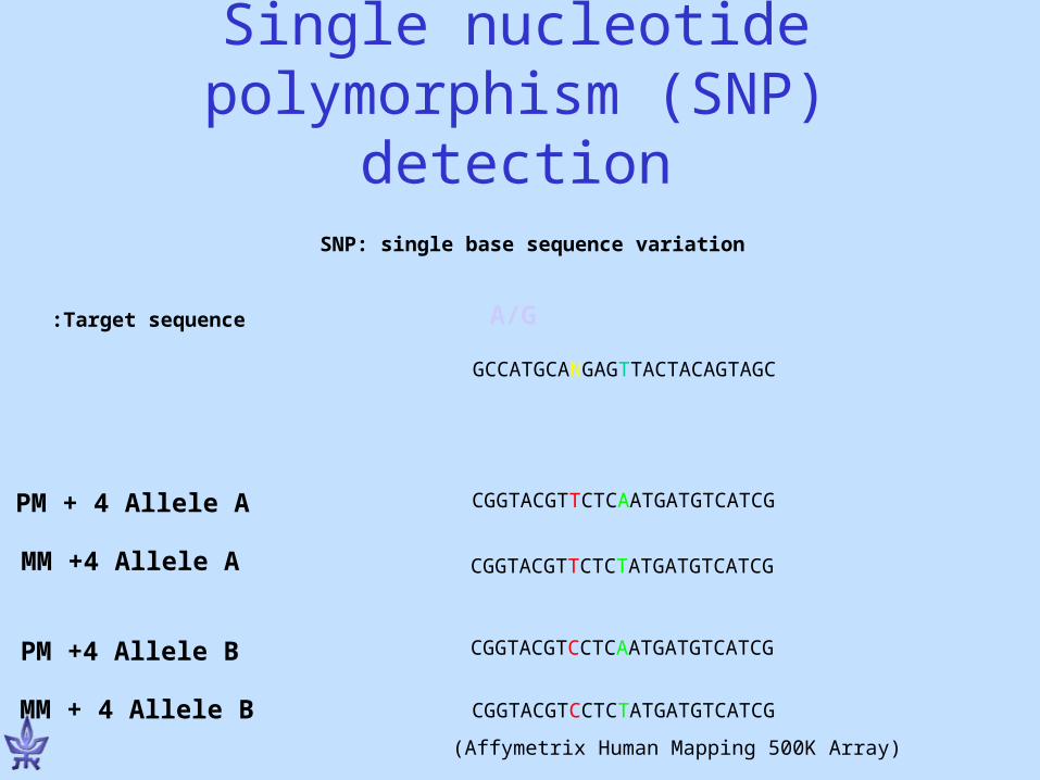
Single nucleotide polymorphism (SNP) detection
GCCATGCANGAGTTACTACAGTAGC
CGGTACGTTCTCAATGATGTCATCG
A/G
CGGTACGTTCTCTATGATGTCATCG
PM + 4 Allele A
MM +4 Allele A
CGGTACGTCCTCAATGATGTCATCG
CGGTACGTCCTCTATGATGTCATCG
PM +4 Allele B
MM + 4 Allele B
(Affymetrix Human Mapping 500K Array)
Target sequence:
SNP: single base sequence variation
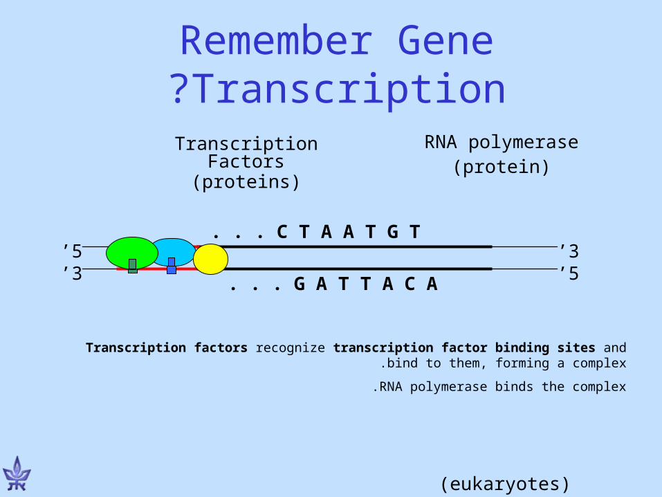
Remember Gene Transcription?
Transcription factors recognize transcription factor binding sites and bind to them, forming a complex.
RNA polymerase binds the complex.
3’5’
5’3’
G A T T A C A. . .
C T A A T G T. . .
Transcription Factors
(proteins)
RNA polymerase(protein)
(eukaryotes)
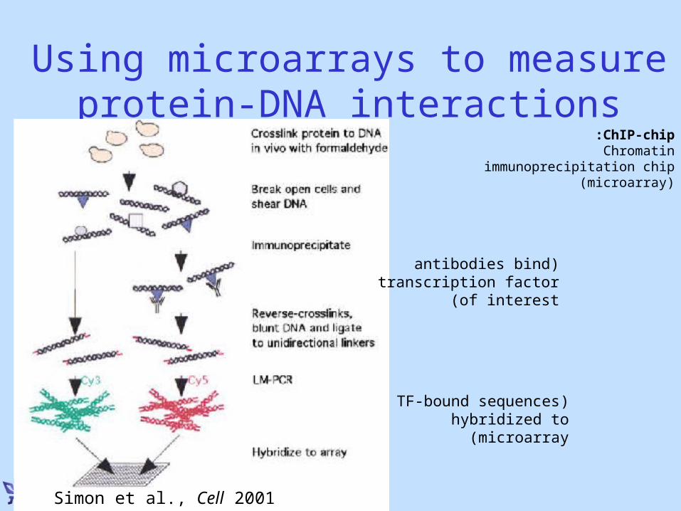
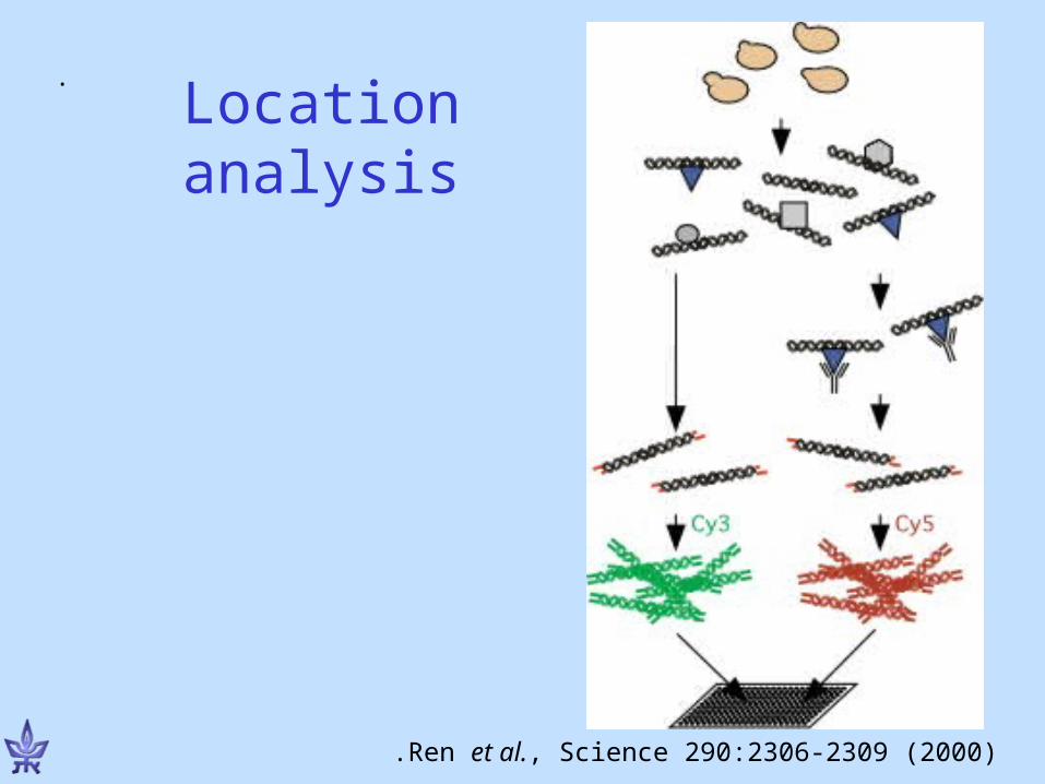
Using microarrays to measure protein-DNA interactions
Simon et al., Cell 2001
ChIP-chip: Chromatin immunoprecipitation chip
(microarray)
(antibodies bind transcription factor of interest )
(TF-bound sequences hybridized to microarray)
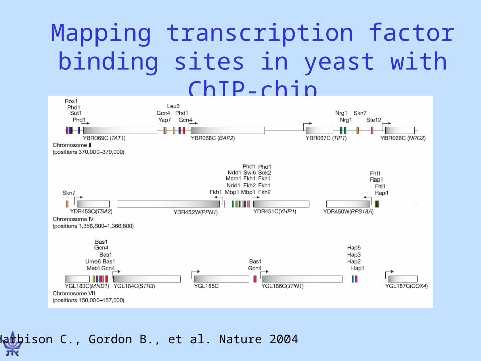
Mapping transcription factor binding sites in yeast with ChIP-chip
Harbison C., Gordon B., et al. Nature 2004
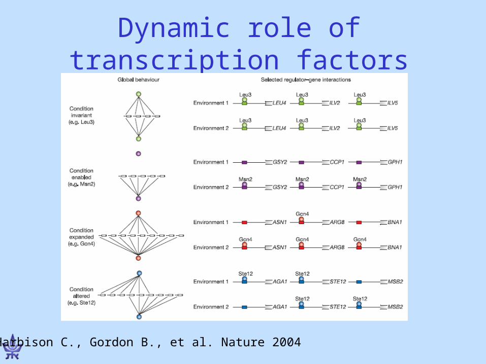
Dynamic role of transcription factors
Harbison C., Gordon B., et al. Nature 2004
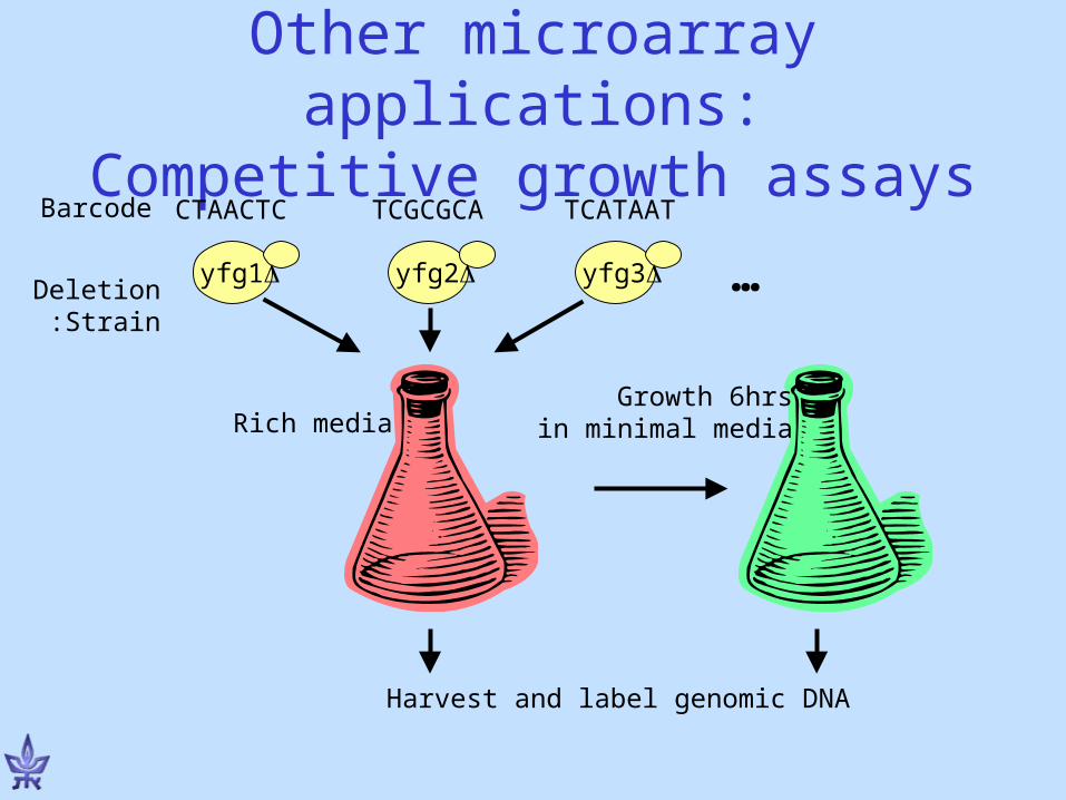
Other microarray applications:Competitive growth assays
yfg1 yfg2 yfg3
CTAACTC TCGCGCA TCATAATBarcode
DeletionStrain:
Growth 6hrsin minimal mediaRich media
…
Harvest and label genomic DNA
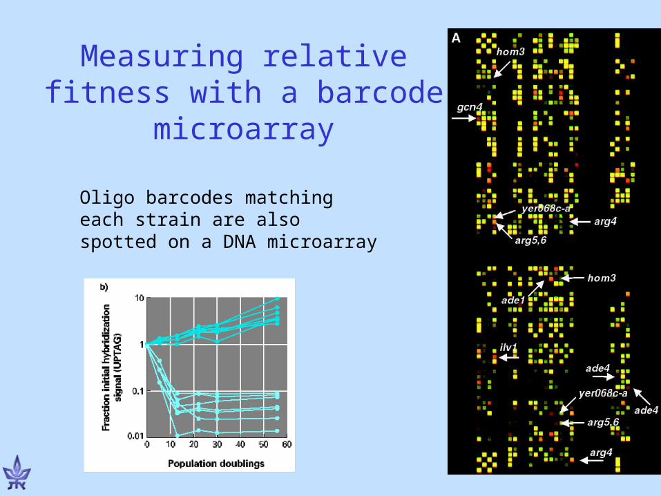
Measuring relative fitness with a barcode microarray
Oligo barcodes matching each strain are also spotted on a DNA microarray
Protein MicroarraysProtein Microarrays• Protein microarrays are lagging behind DNA
microarrays
• Same idea but immobilized elements are proteins instead of nucleic acids
• Number of elements (proteins) on current protein microarrays are limited (approx. 500)
• Antibodies for high density microarrays have limitations (cross-reactivities)
• Aptamers or engineered antibodies/proteins may be viable alternatives
(Aptamers:RNAs that bind proteins with high specificity and affinity)
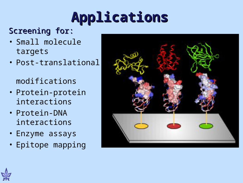
ApplicationsApplicationsScreening for:Screening for:• Small molecule
targets• Post-translational
modifications• Protein-protein
interactions• Protein-DNA
interactions• Enzyme assays• Epitope mapping
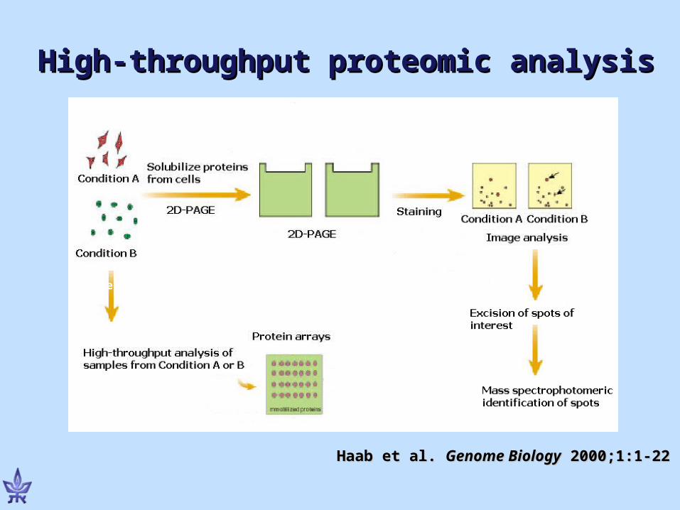
High-throughput proteomic analysisHigh-throughput proteomic analysis
Haab et al. Haab et al. Genome BiologyGenome Biology 2000;1:1-22 2000;1:1-22
Label all Proteins in Mixture
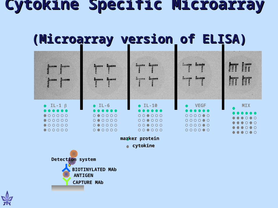
marker proteinmarker protein
cytokinecytokine
VEGFIL-10IL-6IL-1 MIX
BIOTINYLATED MAb
CAPTURE MAb
ANTIGEN
Detection system
Cytokine Specific Microarray Cytokine Specific Microarray (Microarray version of ELISA)(Microarray version of ELISA)
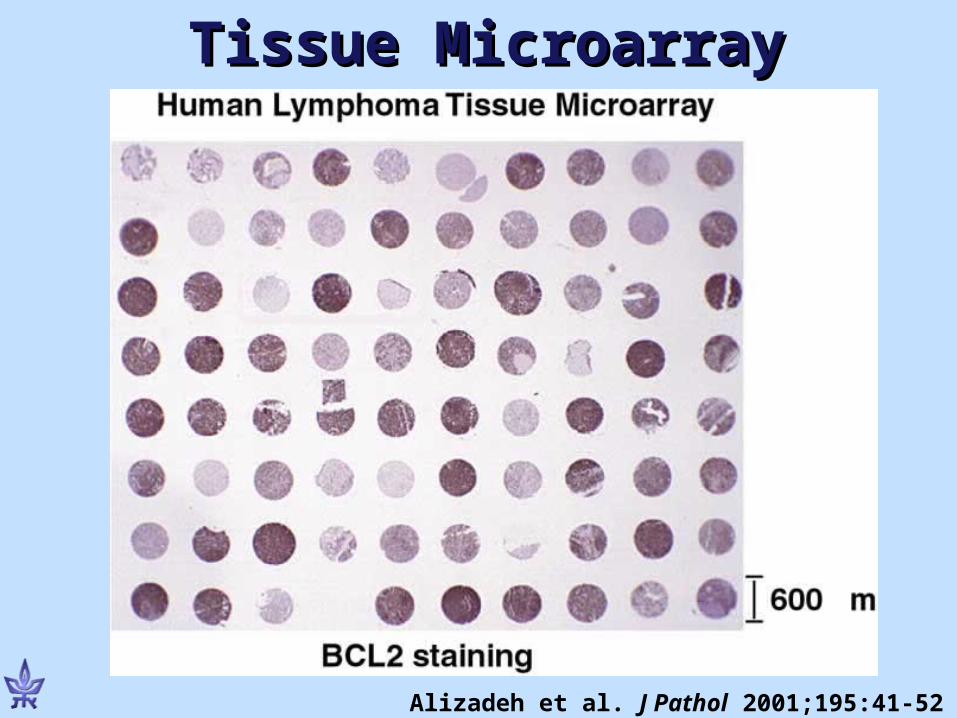
Tissue MicroarraysTissue Microarrays
• Printing on a slide tiny amounts of tissue
• Array many patients in one slide (e.g. 500)
• Process all at once (e.g. immunohistochemistry)
• Works with archival tissue (paraffin blocks)
34
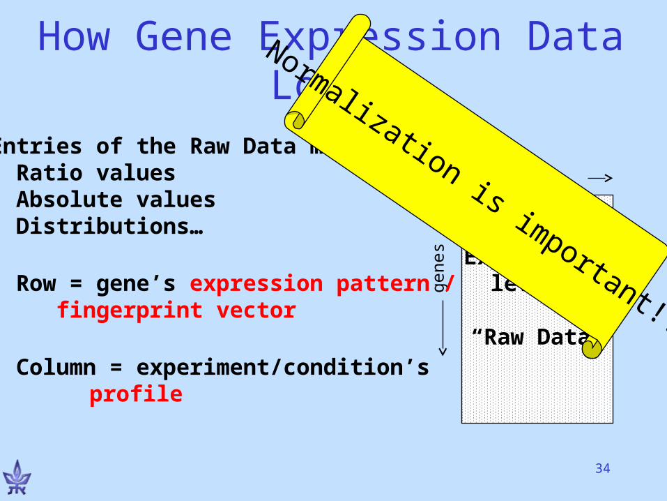
How Gene Expression Data Looks
Expression levels,
“Raw Data”
conditions
genes
Entries of the Raw Data matrix:• Ratio values• Absolute values• Distributions…
• Row = gene’s expression pattern /fingerprint vector
• Column = experiment/condition’s profile
Normalization is important!!
35
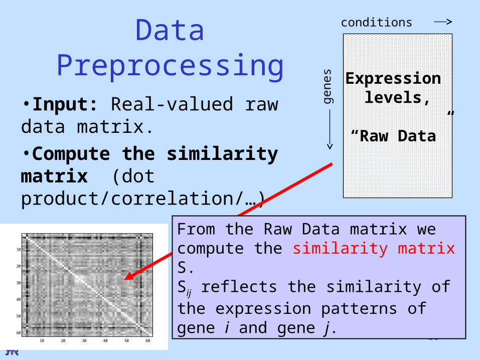
Data PreprocessingExpression
levels,
“Raw Data”
conditions
genes
•Input: Real-valued raw data matrix.•Compute the similarity matrix (dot product/correlation/…)
10 20 30 40 50 60
10
20
30
40
50
60
From the Raw Data matrix we compute the similarity matrix S.Sij reflects the similarity of the expression patterns of gene i and gene j.
36
DNA chips: Applications
• Deducing functions of unknown genes (similar expression pattern similar function)• Identifying disease profiles• Deciphering regulatory mechanisms (co-expression co-regulation).• Classification of biological conditions • Genotyping•Drug development•…
Analysis requires clustering of genes/conditions.
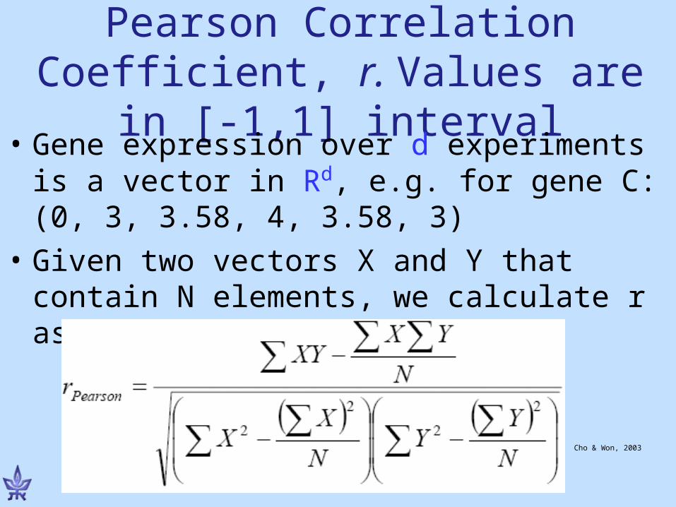
Pearson Correlation Coefficient, r. Values are in [-
1,1] interval• Gene expression over d experiments is a
vector in Rd, e.g. for gene C: (0, 3, 3.58, 4, 3.58, 3)
• Given two vectors X and Y that contain N elements, we calculate r as follows:
Cho & Won, 2003
Intuition for Pearson Correlation Coefficient
r(v1,v2) close to 1: v1, v2 highly correlated.r(v1,v2) close to -1: v1, v2 anti correlated.r(v1,v2) close to 0: v1, v2 not correlated.
Pearson Correlation and p-Values
When entries in v1,v2 are distributed according to normal distribution, can assign(and efficiently compute) p-Values for a given result.
These p-Values are determined by the Pearson correlation coefficient, r, and thedimension, d, of the vectors.For same r, vectors of higher dimension willbe assigned more significant (smaller) p-Value.
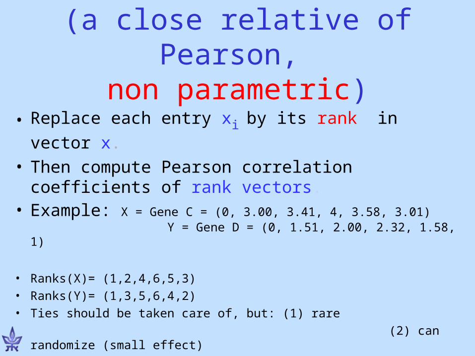
• Replace each entry xi by its rank in vector x.
• Then compute Pearson correlation coefficients of rank vectors.
• Example: X = Gene C = (0, 3.00, 3.41, 4, 3.58, 3.01) Y = Gene D = (0, 1.51, 2.00, 2.32, 1.58, 1)
• Ranks(X)= (1,2,4,6,5,3)• Ranks(Y)= (1,3,5,6,4,2)• Ties should be taken care of, but: (1) rare (2) can randomize (small effect)
Spearman Rank Order Coefficient
(a close relative of Pearson, non parametric)
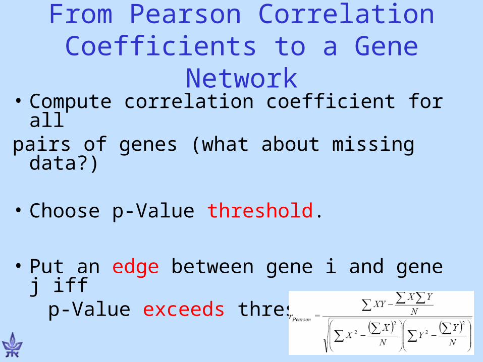
From Pearson Correlation Coefficients to a Gene Network
• Compute correlation coefficient for allpairs of genes (what about missing
data?)
• Choose p-Value threshold.
• Put an edge between gene i and gene j iff
p-Value exceeds threshold.

42
Clustering: Objective
Group elements (genes) to clusters satisfying:
• Homogeneity: Elements inside a cluster are highly similar to each other.
• Separation: Elements from different clusters have low similarity to each other.
45
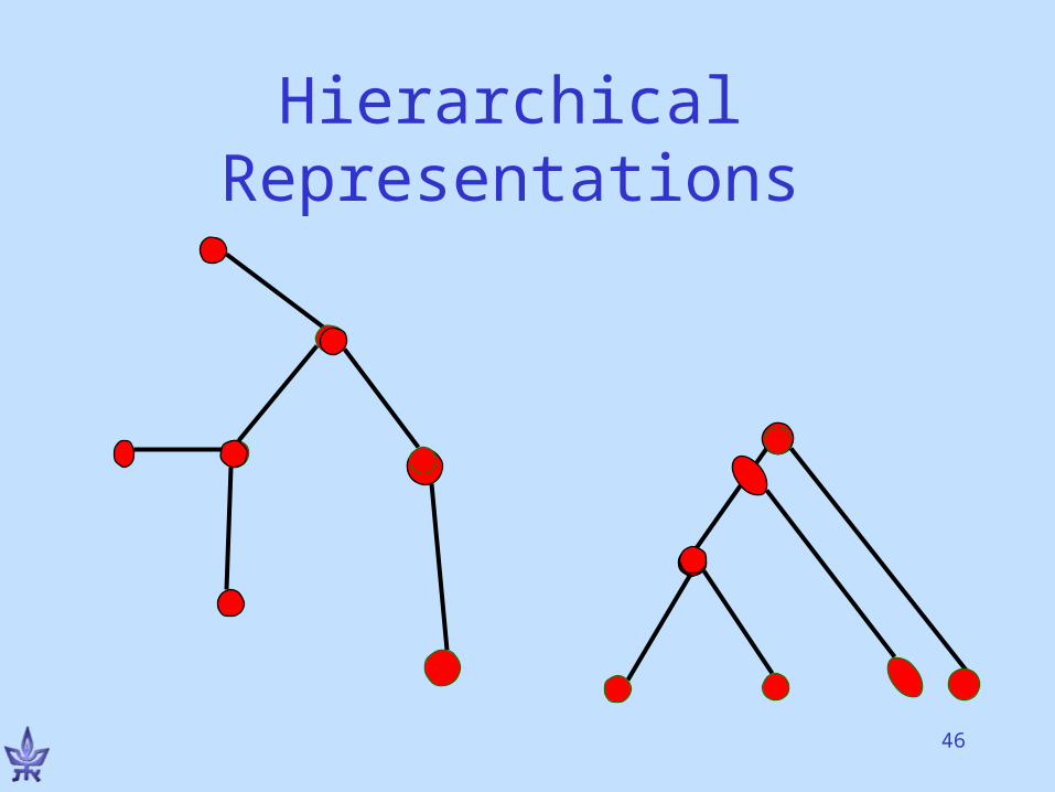
An Alternative ViewForm a tree-hierarchy of the input elements satisfying:
• More similar elements are placed closer along the tree.
• Or: Tree distances reflect element similarity
•Note: No explicit partition into clusters.
47
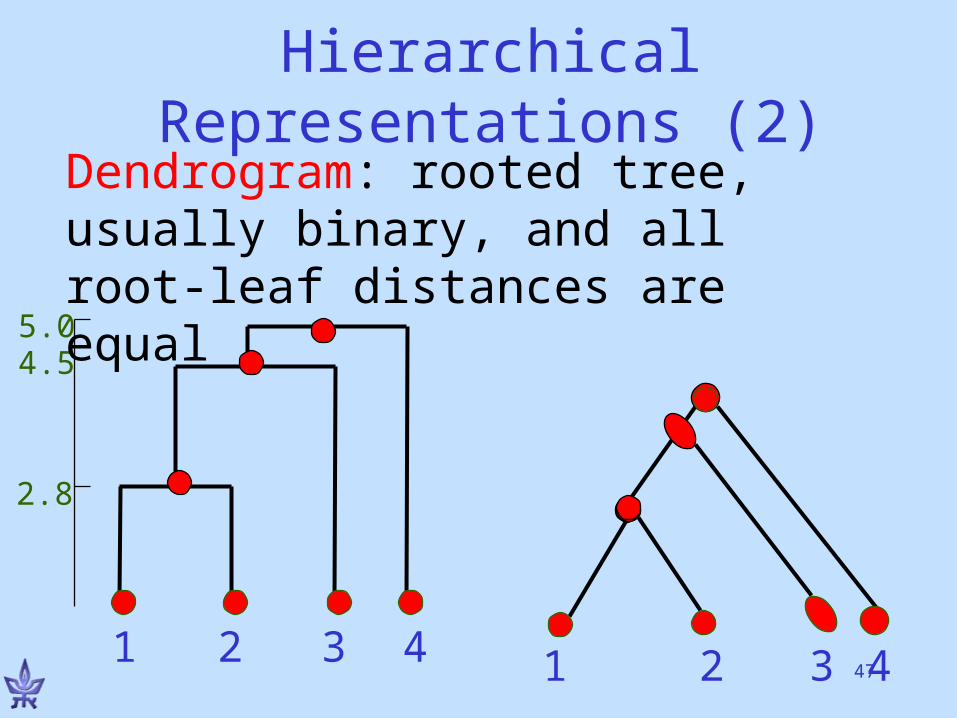
Hierarchical Representations (2)
1 3 421 3 42
2.8
4.55.0
Dendrogram: rooted tree, usually binary, and all root-leaf distances are equal
48
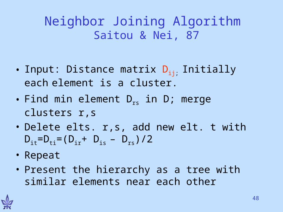
Neighbor Joining Algorithm Saitou & Nei, 87
• Input: Distance matrix Dij; Initially each
element is a cluster.
• Find min element Drs in D; merge clusters r,s
• Delete elts. r,s, add new elt. t with Dit=Dti=(Dir+ Dis – Drs)/2
• Repeat• Present the hierarchy as a tree with similar
elements near each other
49
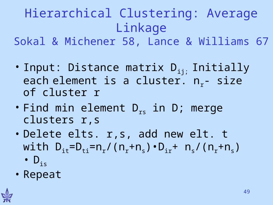
Hierarchical Clustering: Average LinkageSokal & Michener 58, Lance & Williams 67
• Input: Distance matrix Dij; Initially each element is a cluster. nr- size of cluster r
• Find min element Drs in D; merge clusters r,s
• Delete elts. r,s, add new elt. t with Dit=Dti=nr/(nr+ns)•Dir+ ns/(nr+ns) • Dis
• Repeat
50
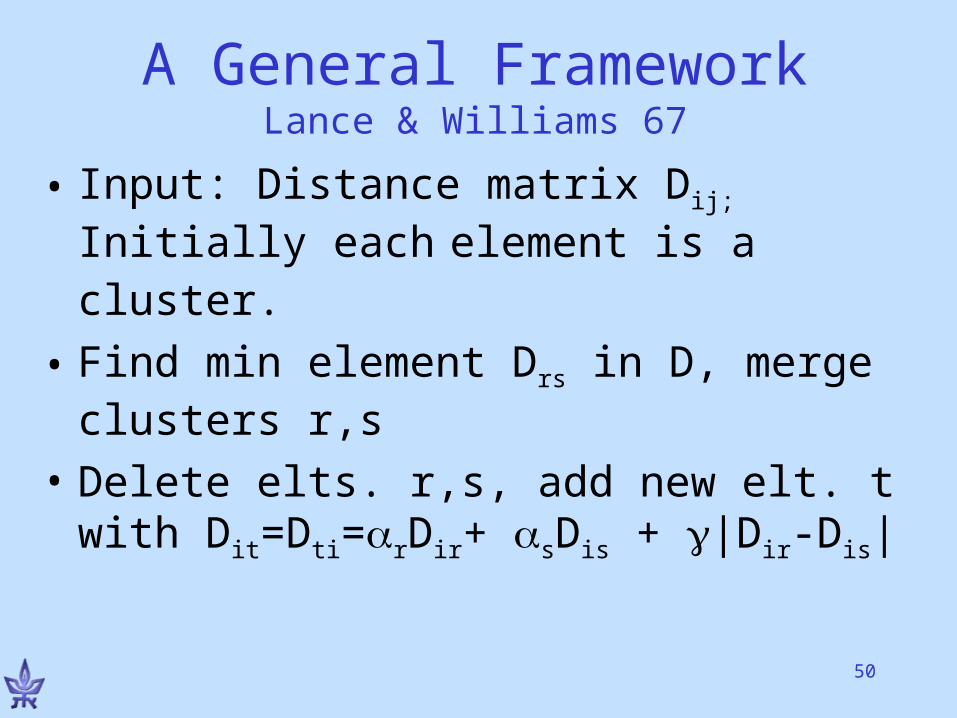
A General FrameworkLance & Williams 67
• Input: Distance matrix Dij; Initially each
element is a cluster.
• Find min element Drs in D, merge clusters r,s
• Delete elts. r,s, add new elt. t with Dit=Dti=rDir+ sDis + |Dir-Dis|
51
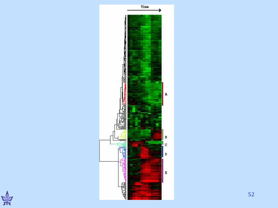
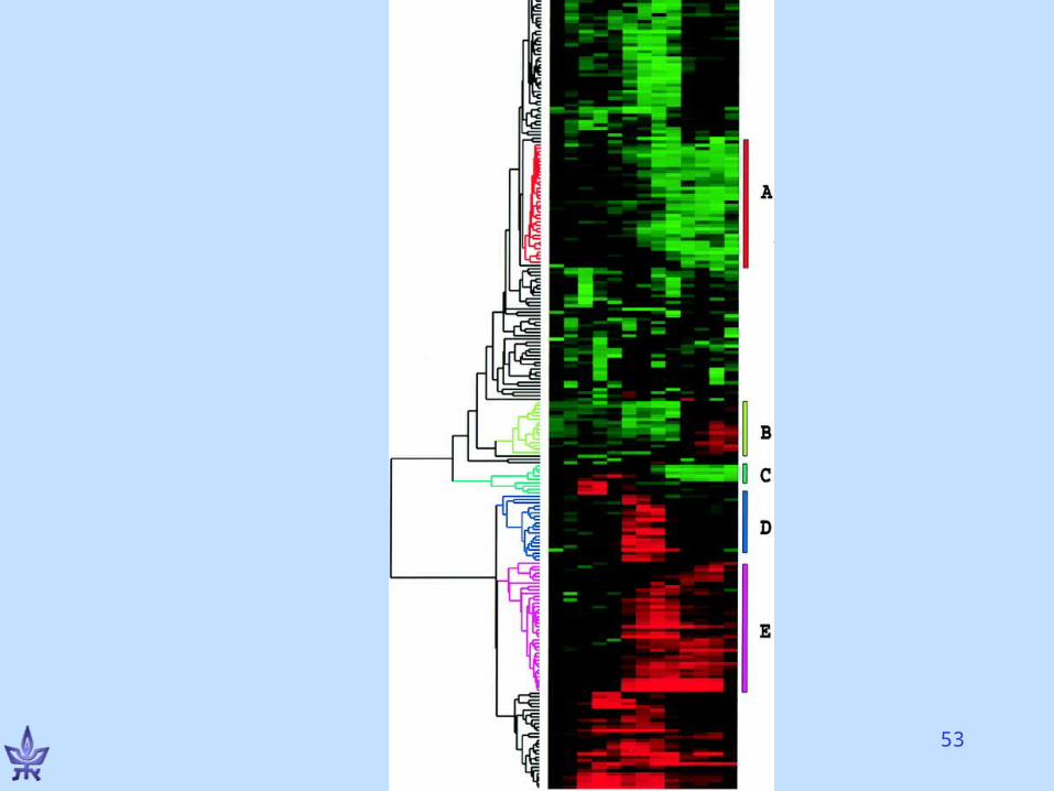
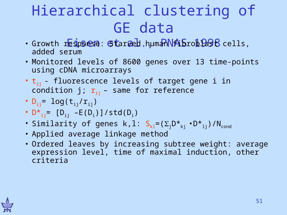
Hierarchical clustering of GE data
Eisen et al., PNAS 1998• Growth response: Starved human fibroblast cells, added serum
• Monitored levels of 8600 genes over 13 time-points using cDNA microarrays
• tij - fluorescence levels of target gene i in condition j; rij – same for reference
• Dij= log(tij/rij)
• D*ij= [Dij –E(Di)]/std(Di)
• Similarity of genes k,l: Skl=(jD*kj •D*lj)/Ncond
• Applied average linkage method• Ordered leaves by increasing subtree weight: average
expression level, time of maximal induction, other criteria
54
Comments
• Distinct measurements of same genes cluster together
• Genes of similar function cluster together
• Many cluster-function specific insights• Interpretation is a REAL biological
challenge
55
More on hierarchical methods
• All methods described above – agglomerative
• An alternative approach: Divisive• Advantages:
– gives a single coherent global picture– Intuitive for biologists (from phylogeny)
• Disadvantages:– no single partition; no specific clusters– Forces all elements to fit a tree
hierarchy
57
Clustering: ObjectiveGroup elements (genes) to clusters satisfying:
• Homogeneity: Elements inside a cluster are highly similar to each other.
• Separation: Elements from different clusters have low similarity to each other.
•Needs formal objective functions•Most useful versions are NP-hard.
58
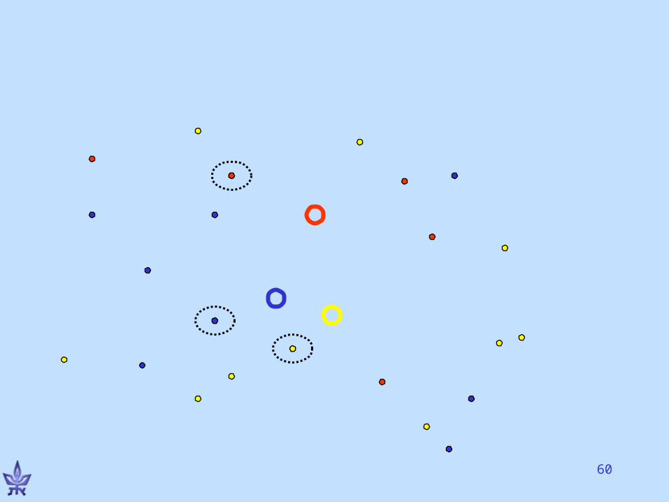
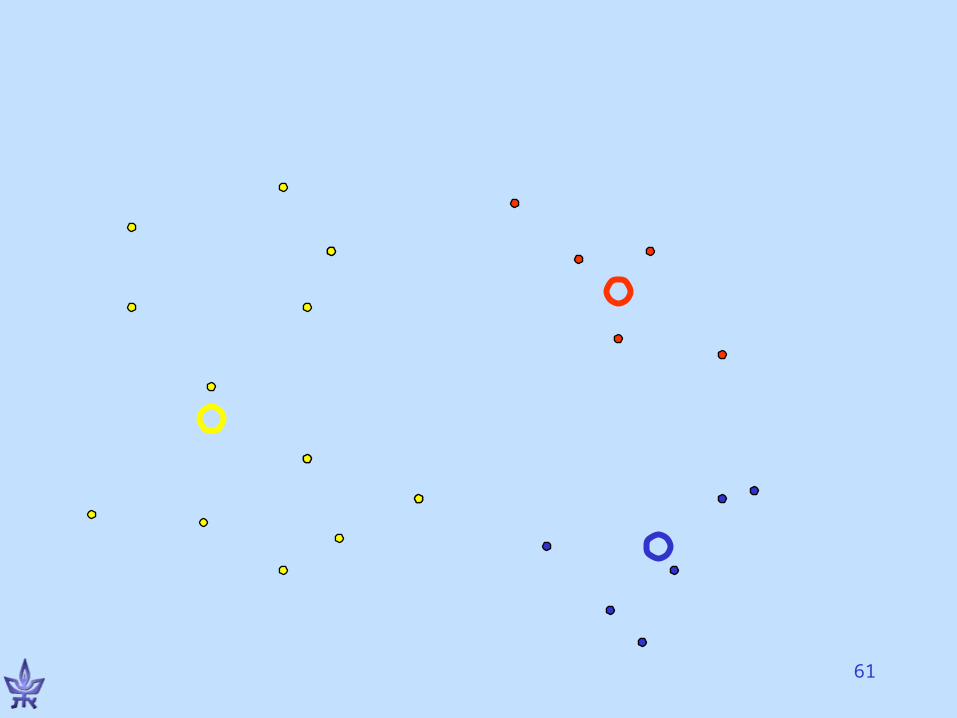
K-means clusteringMacQueen, 65
• Initialize an arbitrary partition P into k clusters C1 ,…, Ck.
• For cluster Cj, element i Cj, EP(i, Cj) = cost of soln. if i is moved to cluster Cj. Pick EP(r, Cs) that is minimum; move r to cluster Cs if the new partition is better than P
• Repeat until no improvement possible• Requires knowledge of k
59
K-means variations• Input: vector vi for each element i• Compute a centroid cp for each cluster Cp, e.g., gravity
center = average vector• Solution cost: clusters pi in cluster pd(vi,cp)• EP(i,j)= change in soln. cost if i is moved to cluster Cj. • Parallel version: move each elt. to the cluster with the
closest centroid simultaneously• Sequential version: one elt. each time• “moving centers” approach• Objective = homogeneity only (k fixed)• Variations for changing k
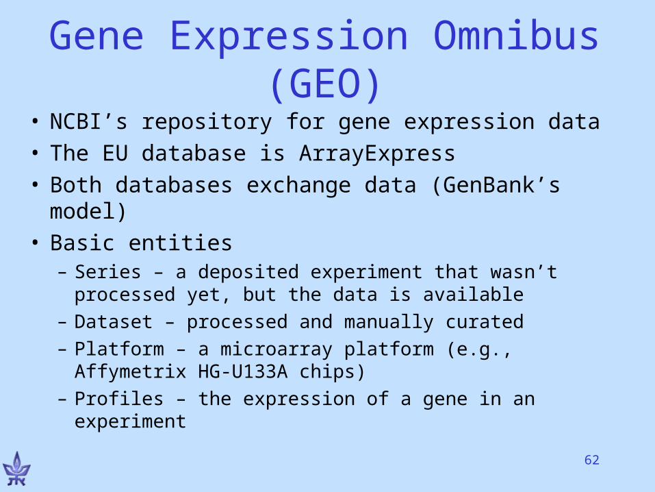
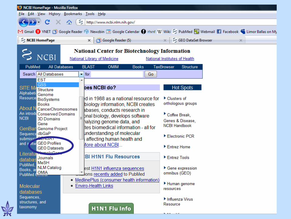
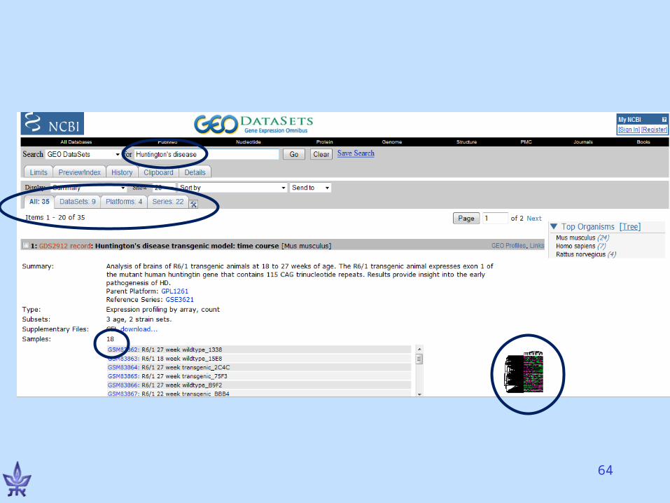
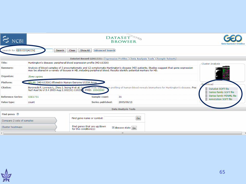
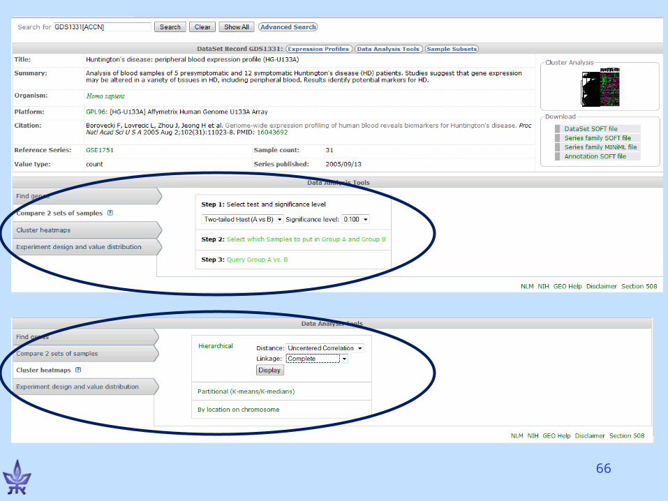
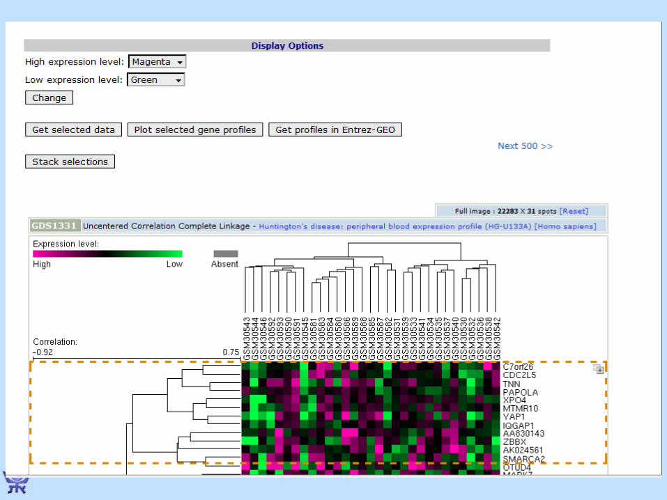
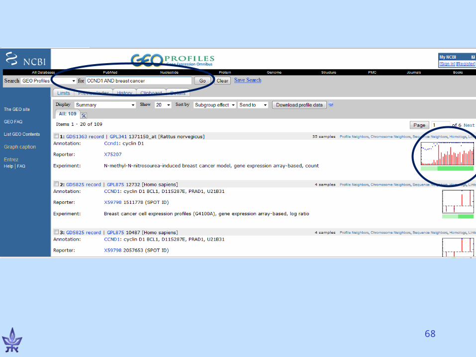
Gene Expression Omnibus (GEO)
• NCBI’s repository for gene expression data• The EU database is ArrayExpress• Both databases exchange data (GenBank’s
model)• Basic entities
– Series – a deposited experiment that wasn’t processed yet, but the data is available
– Dataset – processed and manually curated– Platform – a microarray platform (e.g., Affymetrix HG-
U133A chips)– Profiles – the expression of a gene in an experiment
62
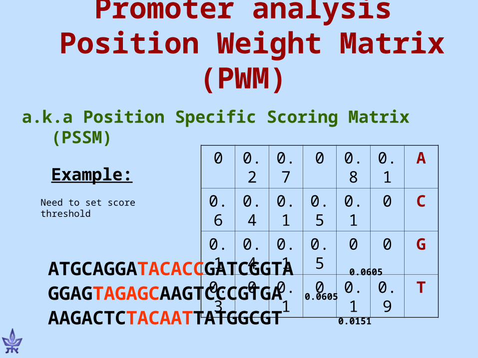
Promoter analysis Position Weight Matrix
(PWM)a.k.a Position Specific Scoring Matrix
(PSSM)
Example: A0.10.800.70.20
C00.10.50.10.40.6
G000.50.10.40.1
T0.90.100.100.3
ATGCAGGATACACCGATCGGTA 0.0605
GGAGTAGAGCAAGTCCCGTGA 0.0605
AAGACTCTACAATTATGGCGT 0.0151
Need to set score threshold
Computational approaches to promoter analysis
• Look for overrepresented BSs in groups of promoters– Obtained by clustering expression profiles– Of genes with a common known function (e.g.
from GO annotations)– From chip2 data – requires knowledge of the TF,
and an antibody.
- Use a combination of sources
• De-novo or using known TF signatures
ATM-dependent Transcriptional Response to
Ionizing Radiation• DNA damage response modulates many
signaling pathways, including lesion processing, repair, cell cycle checkpoints and apoptotic pathway.
• ATM protein kinase is a master regulator of cellular response to double strand breaks.
Goal: identify the transcriptional network.
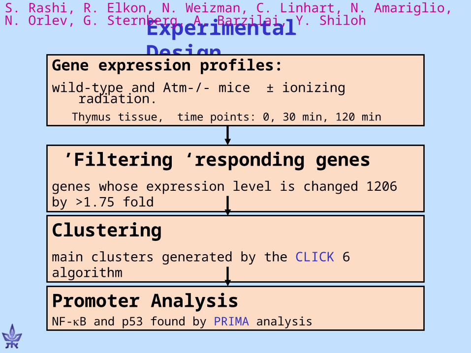
Experimental Design
Gene expression profiles:wild-type and Atm-/- mice ± ionizing radiation.
Thymus tissue, time points: 0, 30 min, 120 min
S. Rashi, R. Elkon, N. Weizman, C. Linhart, N. Amariglio, N. Orlev, G. Sternberg, A. Barzilai, Y. Shiloh
Filtering ‘responding genes ’1206 genes whose expression level is changed by >1.75 fold
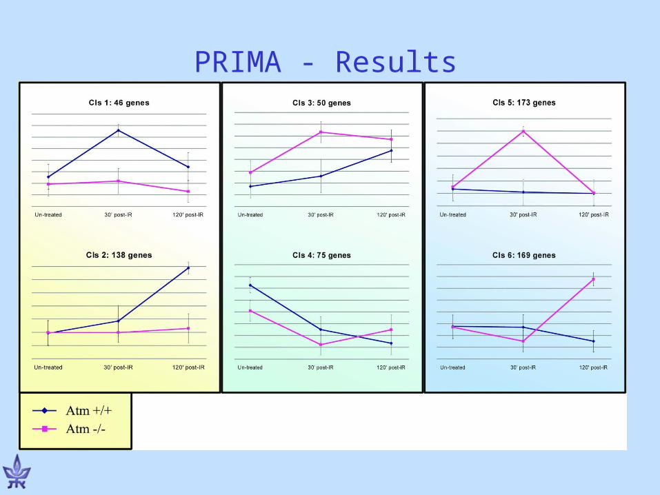
Clustering6 main clusters generated by the CLICK algorithm
Promoter AnalysisNF-B and p53 found by PRIMA analysis
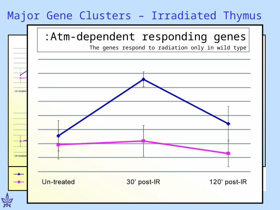
Atm-dependent responding genes:The genes respond to radiation only in wild type
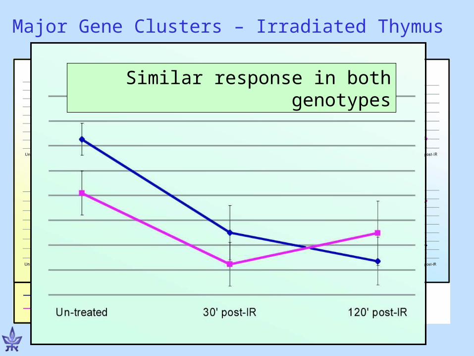
Major Gene Clusters – Irradiated Thymus
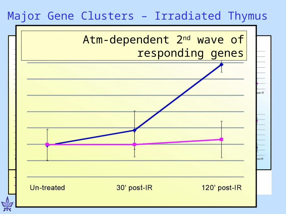
Atm-dependent 2nd wave of responding genes
Major Gene Clusters – Irradiated Thymus
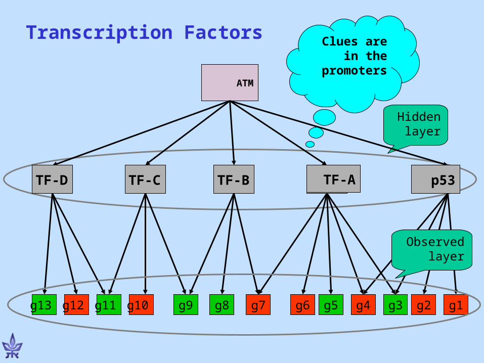
? ? ? ?
Hidden layer
?
ATM
g3g13 g12 g10 g9 g1g8 g7 g6 g5 g4g11 g2
Observed layer
Clues are in the
promoters
Transcription Factors
p53TF-C TF-B TF-ATF-D
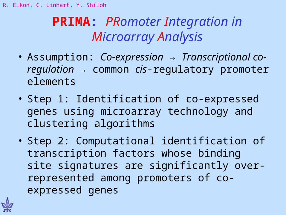
PRIMA: PRomoter Integration in Microarray Analysis
• Assumption: Co-expression → Transcriptional co-regulation → common cis-regulatory promoter elements
• Step 1: Identification of co-expressed genes using microarray technology and clustering algorithms
• Step 2: Computational identification of transcription factors whose binding site signatures are significantly over-represented among promoters of co-expressed genes
R. Elkon, C. Linhart, Y. Shiloh
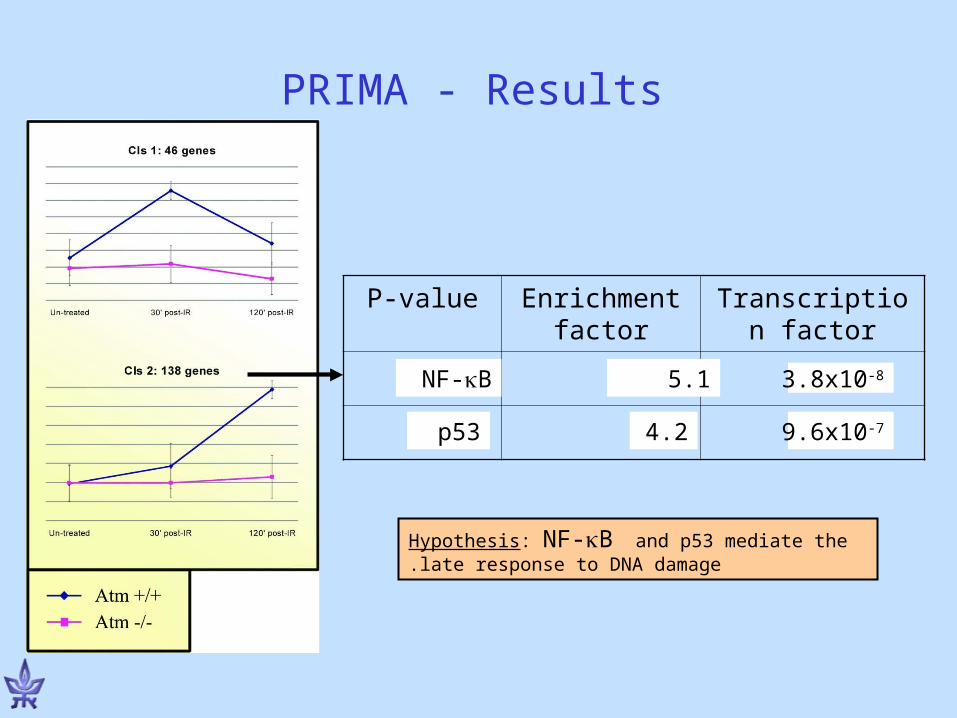
Transcription factor
Enrichment factor
P-value
PRIMA - Results
NF-B 5.1 3.8x10⁻⁸
p53 4.2 9.6x10⁻⁷
Hypothesis: NF-B and p53 mediate the late response to DNA damage.
Molecular Classification of Cancer: Class Discovery and
Class Prediction by Gene Expression Monitoring
Golub TR, Slonim DK, Tamayo P, Huard C, Gaasenbeek M, Mesirov JP, Coller H, Loh ML, Downing JR, Caligiuri MA, Bloomfield CD, Lander ES.
Science 286 (Oct 1999) 531-537Computational paper: Class Prediction and Discovery Using Gene Expression Data Donna K. Slonim, Pablo Tamayo, Jill P. Mesirov, Todd R. Golub, Eric S. Lander Proc. RECOMB 2000
ppt Source: Elashof-Horvath UCLA course, Statistical Analysis of DNA Microarray Data http://www.genetics.ucla.edu/horvathlab/Biostat278/Biostat278.htm
Background: Cancer Classification
• Cancer classification is central to cancer treatment;
• Traditional cancer classification methods: by sites; by morphology, etc;
• Limitations of morphology classification: tumors of similar histopathological appearance can have significantly different clinical courses and response to therapy;
• Traditionally cancer classification relied on specific biological insights
• Challenges: – finer classification of morphologically similar tumors at
the molecular level; – systematic and unbiased approaches;
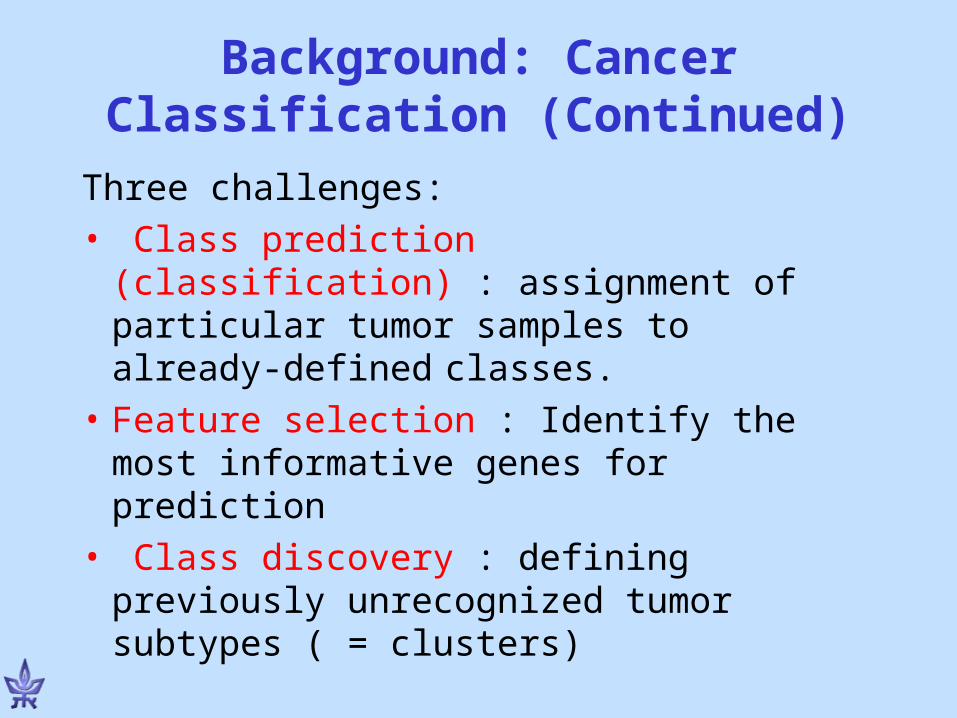
Background: Cancer Classification (Continued)
Three challenges:• Class prediction (classification) :
assignment of particular tumor samples to already-defined classes.
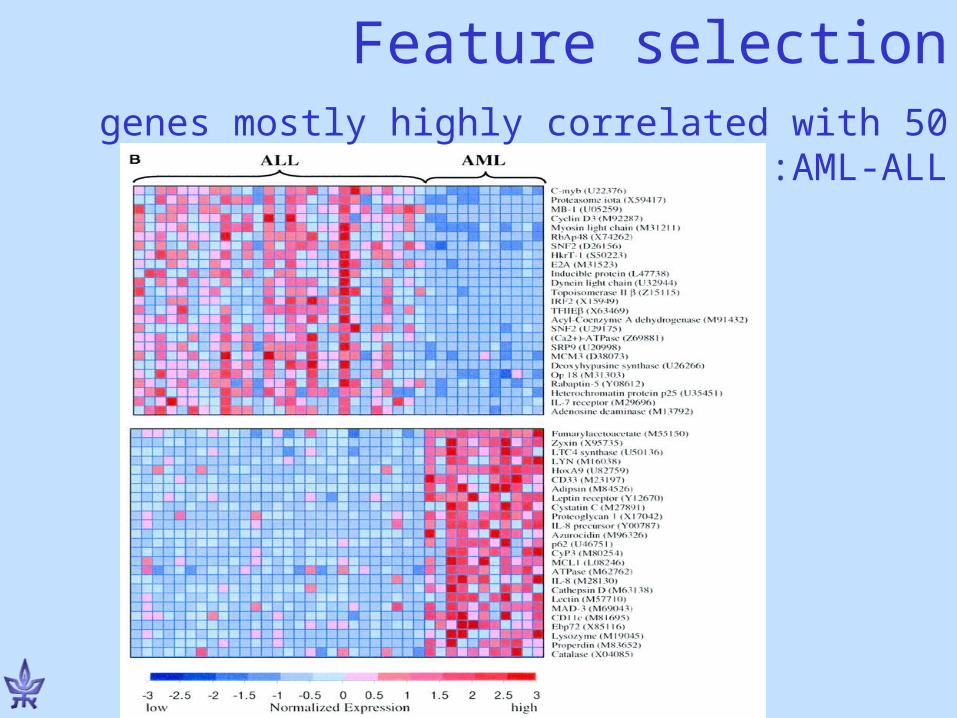
• Feature selection : Identify the most informative genes for prediction
• Class discovery : defining previously unrecognized tumor subtypes ( = clusters)
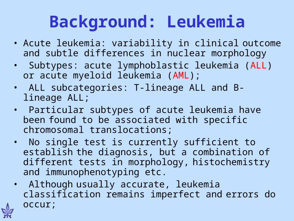
Background: Leukemia• Acute leukemia: variability in clinical outcome and
subtle differences in nuclear morphology• Subtypes: acute lymphoblastic leukemia (ALL) or
acute myeloid leukemia (AML);• ALL subcategories: T-lineage ALL and B-lineage
ALL;• Particular subtypes of acute leukemia have been
found to be associated with specific chromosomal translocations;
• No single test is currently sufficient to establish the diagnosis, but a combination of different tests in morphology, histochemistry and immunophenotyping etc.
• Although usually accurate, leukemia classification remains imperfect and errors do occur;
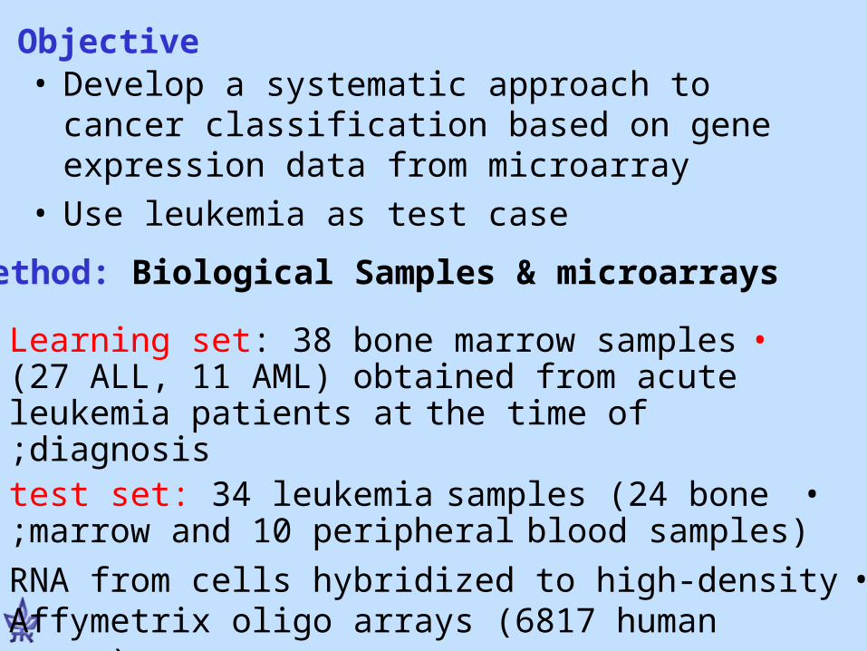
Objective• Develop a systematic approach to cancer
classification based on gene expression data from microarray
• Use leukemia as test case
Method: Biological Samples & microarrays
•Learning set: 38 bone marrow samples (27 ALL, 11 AML) obtained from acute leukemia patients at the time of diagnosis;
• test set: 34 leukemia samples (24 bone marrow and 10 peripheral blood samples);
•RNA from cells hybridized to high-density Affymetrix oligo arrays (6817 human genes)
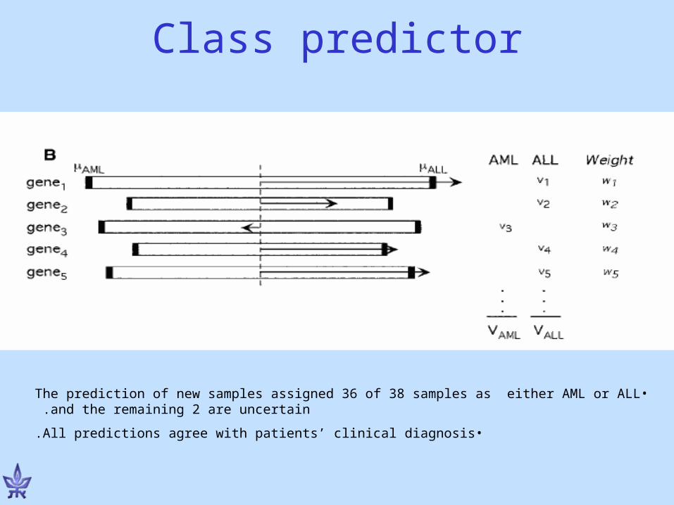
Class predictor
•The prediction of new samples assigned 36 of 38 samples as either AML or ALL and the remaining 2 are uncertain .
•All predictions agree with patients’ clinical diagnosis.