GENDER DIFFERENCES IN THE EFFECTS OF VOCATIONAL TRAINING: CONSTRAINTS ON WOMEN AND DROPOUT BEHAVIOR¶

Yoonyoung Cho, World Bank

Davie Kalomba, Malawi National AIDS Commission

Ahmed Mushfiq Mobarak, Yale University§

Victor Orozco, World Bank

Derek Wolfson, UC Berkeley

June 2016

Abstract We provide experimental evidence on the effects of vocational and entrepreneurial training for Malawian youth in an environment where access to schooling and formal sector employment is extremely low. The training results in skills development, continued investment in human capital and improved well-being, with more positive effects for men, but no improvements in labor market outcomes in the short-run. We find that women make decisions in a more constrained environment, and their participation is affected by family obligations. We also find that participation is more expensive for women compared to their male counterparts, resulting in a worse training experience. Additionally, we track a large fraction of program dropouts – a common phenomenon in the training evaluation literature – which allows us to examine the determinants and consequences of the dropout decision and how it mediates the effects of such programs.

Keywords: apprenticeship training; vulnerable youth; gender; dropouts; Malawi

JEL codes: O15, J24, I15

¶ The authors thank Sangeeta Raja, Rachel Hoy, Maria Jones, Sylvan Herskowitz, Clara Hopler, Emmanuel Kanike, Pavel

Luengas, Julia Brown, Tatyana Zelenska for their excellent work that made this evaluation possible. We thank the World Bank’s Spanish Impact Evaluation Fund, Youth Employment Network, and the UK Department for International Development for financial support for the research. The intervention was funded by the Global Fund. The views expressed herein are those of the authors and should not be attributed to the World Bank, its executive directors, or the countries they represent.

§ Corresponding Author. Email: ahmed.mobarak@yale.edu. Phone: +1-203-432-5787

1

1. Introduction

Providing training to help individuals acquire skills and increase their productivity is one

way to increase earnings and employment in both developed and less-developed nations (The

World Bank 2004). Job training programs have therefore emerged as a widely studied policy

instrument. Due to data availability, however, the evaluation of such programs has been

mostly limited to developed countries. (e.g. Lynch 1992; Bartel 1995; Heckman, Lochner, and

Taber 1998; Frazis and Loewenstein 2005; Kluve 2010; Hirshleifer et al. 2015). Most evaluations

rely on non-experimental techniques, including conditioning on observables to limit selection

bias (Friedlander, Greenberg, and Robins 1997; Heckman et al. 2000), parametric selection

correction methods (Heckman et al. 1998), and propensity score matching and duration

analysis (Bring and Carling 2000; Gerfin and Lechner 2002; Sianesi 2004; Chong and Galdo

2006; Biewen et al. 2007; Jespersen, Munch, and Skipper 2008).

We report the results of a randomized control trial to evaluate an entrepreneurship and

vocational training program in Malawi. Over 80-percent of the workforce in Sub-Saharan

Africa engages in self-employment in small businesses and household enterprises (Gindling

and Newhouse 2014), which makes entrepreneurship and vocational training more relevant in

this context than formal job training programs (Malamud and Pop-Eleches 2010). In Banerjee

and Duflo’s (2007) 18-country, sample-based description of the lives of the poor, they report

that a “large fraction of the poor act as entrepreneurs” and are self-employed, with many

operating non-agricultural businesses. In contrast, formal employment opportunities are

relatively scarce in the developing world (The World Bank 2012b).

The program we evaluate was designed to provide apprenticeship rather than classroom-

based training. It targeted people aged 15-24, because the youth often lack the formal

education or skills required to access salaried employment in Malawi. A growing number of

development-aid agencies around the world have attempted to reduce youth unemployment

through on-the-job training and vocational programs. Examples of the emphasis on vocational

training are found in Tanzania, South Korea, and Indonesia, where some programs have

attempted to shift secondary school curricula away from general education and towards

vocational training (Newhouse and Suryadarma 2011). The program we evaluate in Malawi

consisted of 1900 participants from 28 districts who received on-the-job training through

placement as apprentices to master craftspeople (MC) in their preferred area of interest.

2

Apprenticeships of this type are common in Sub-Saharan Africa as a way for individauls

without access to formal education to gain employable skills (Biavaschi et al. 2012). Despite

their popularity, virtually no evidence exists on the effects of such programs.1

To our knowledge, only three papers have previously addressed the effects of vocational

training programs in less-developed countries using experimental evidence.2 Maitra and Mani

(2015) find that women who participated in a sewing training program in India were more

likely to be employed, worked more hours and earned more money in the short- and medium-

term. Bandiera et al. (2012) evaluate the combined effects of life-skills and vocational (but not

on-the-job) training on health-related sexual behavior and employment for adolescent girls in

Uganda. They find that this dual-pronged intervention leads to more involvement in income

generating activities, but, given their setting, cannot separate out the effects of the vocational

training from the life-skills training. Chakravarty et al. (2014) evaluate the effects of a two-step

training program for young women in Liberia that consists of classroom-based training in six

trades and job-placement component. These authors find this program to increase

employment and earnings significantly in the post-study period. Our study expands on this set

of literature by examining the effects on-the-job apprenticeship training in a less-developed

country for both men and women across a wide variety of occupations.

A related suite of literature exists for both classroom and on-the-job training in middle-

income countries in Central and South America. Attanasio et al. (2011), Attanasio et al. (2015)

and Alzúa et al. (2016) find that vocational training for youth has fairly large effects on wages

and employment and identify that these effects persist in the medium- to long-run.3

Conversely, Card et al. (2011), Ibarraran et al. (2014) and Ibarraran et al. (2015) find no effects of

vocational training in the Dominican Republic on employment, yet find modest effects of

training on earnings. In contrast to our study, these authors analyze programs in middle-

1 The ILO (2012) provides an extensive review of qualitative and quantitative studies of informal apprenticeship programs.

Monk et al. (2008), working in Ghana with descriptive data, find that returns to informal apprenticeships are high for those who have low levels of education, but fall as formal education increases. We are unaware of any experimental evidence on apprenticeships.

2 A related (although recent and largely yet unpublished) literature deals with the returns to business training and financial literacy; however these trainings are designed to deliver generic business skills, rather than trade-specific skills. See Cole et al. (2011), Bruhn & Zia (2013), de Mel et al. (2014), Drexler et al. (2014), Karlan & Valdivia (2011), and Calderon et al. (2013).

3 Macours, Schady, and Vakis (2012) evaluate a multi-pronged experiment in Nicaragua that includes a training component for a subset of their sample. All households that received the training program also received a conditional cash transfer and they do not report the effects of this joint treatment on employment-related outcomes.

3

income countries focused on wage employment in large formal sectors. Our study concerns

on-the-job development of technical skills in an environment where self-employment, rather

than wage employment, is the norm.4

A second important contribution of our paper lies in our treatment and analysis of program

dropouts. Several published evaluations of job training programs report that a large fraction of

beneficiaries randomly assigned to receive training fail to show up, or discontinue training

after a short period, which complicates the evaluation method. Heckman et al. (2000),

reviewing five different experimental evaluations of employment and training programs in the

U.S., report dropout rates as high as 79%. The Card et al. (2011) study reports that 17% of their

treatment group failed to attend training, and that follow-up data was not collected on these

people. This can introduce a significant selection bias, which complicates the estimation of the

treatment effects even for studies that start out with experimental data.5

In our study, we experience similarly high rates of dropout among those randomly assigned

to receive training, but we anticipated this problem and tracked down a significant fraction of

the dropouts in our follow-up surveys. This allows us to report intent-to-treat and treatment-

on-treated results (accounting for the dropout decision) that are closer to the pure

experimental estimates. The main short-term effects of training that we report – which are

large, significant increases in the self-reported skills and knowledge that the training was

meant to impart and improvements in trainees’ life satisfaction – are not sensitive to the way

dropouts are handled.

More importantly, we conduct a detailed analysis of why trainees chose to drop out. Since

dropping out is a commonly observed phenomenon across such programs in both developing

and developed nations, it is useful to identify its causes and consequences, in order to better

understand the direction of bias in existing evaluations of training programs stemming from

this specific source of attrition. Our data allow us to characterize whether dropouts in training

are positively or negatively selected. Why potential participants do not take advantage of a

heavily subsidized (or even free) program designed to build their human capital is an important

4 Blattman, Fiala, and Martinez (2014) find that youth given a cash transfer in Uganda invest in vocational training and tools,

which then translate into higher levels of employment and earnings. 5 A large body of literature has devised non-experimental methods to correct for these biases (see: Manski 1989; Manski 1990;

Horowitz and Manski 1998; Heckman, Lalonde, and Smith 1999; Heckman et al. 2000; Horowitz and Manski 2000; DiNardo, McCrary, and Sanbonmatsu 2006; Lee 2009).

4

puzzle worth exploring.6 We collect data on the alternative opportunities and unanticipated

shocks that occurred around the time of program inception to help explain why people choose

to drop out.

These opportunities and constraints affect men and women differently – leading to the

third main contribution of this paper: developing a better understanding of why training

programs may have heterogeneous effects across gender. A growing literature documents

differential treatment effects by gender for a variety of development programs (e.g. see

Bergemann and van den Berg 2008; Attanasio, Kugler, and Meghir 2011; Blattman, Fiala, and

Martinez 2014). We find that improvements in self-reported skills are similar across genders,

however after the completion of the program women are significantly less likely to start a

business and spend relatively less time in skill development post-training than men. Further,

we find that improvements in subjective well-being as a result of participation in the program

are more apparent for men.

These differences are partially explained by the conditions under which women participate

in the training. In this setting, women are more likely than men to participate when

alternative opportunities disappear (e.g. they become unemployed), whereas men’s

participation decisions are not affected by adverse external conditions. At baseline, women are

more likely to report having responsibility for maintaining the household – they have more

dependents and spend more time on domestic chores. As such, women, but not men, cite

‘getting married’ or ‘family obligations’ as the primary reason for not participating in the

program. Additionally, participation in the program is expensive and we find that women

draw upon their savings to participate in the program and that women are less likely to attend

regularly.

It also seems that women sort into occupations where trainers do less for their trainees. As

a result, male trainees are more likely to receive financial help from the MCs and are more

likely to receive paid work from their MC after the training is complete. These results shed

light on the more stringent constraints under which women in developing countries make

6 This is related to a literature that identifies technologies designed to meet pressing needs are often not adopted at rates

commensurate with their potential benefits (Mobarak et al. 2012; Meredith et al. 2013). The case of training appears related to a literature that suggests that the low take-up may signal that the product or service does not work as well as anticipated, given local conditions (e.g. see Ashraf, Giné, and Karlan 2009; Hanna, Duflo, and Greenstone 2016).

5

decisions, and how these conditions inhibit participation in programs that foster skill

acquisition. This is similar to findings from other development programs, such as capital

infusion producing much lower returns for female-owned micro-enterprises in Sri Lanka and

Ghana (Fafchamps et al. 2014; de Mel, McKenzie, and Woodruff 2014) and Muslim women in

India not benefiting from business training, likely due to social restrictions (Field,

Jayachandran, and Pande 2010).

2. Context and Experimental Design

2.1. Background

Malawi is one of the world’s poorest countries. Over 50% of the population falls below the

national poverty line, while GNI per capita is just $360 (The World Bank 2012a).

Unemployment among youth is high – 9.6% for women, 8.5% for men (ILO 2011). Levels of

formal education are low, as about 58% of students drop out after primary school (Aggarwal,

Hofmann, and Phiri 2010). Most youth are particularly vulnerable and rely on low-

productivity subsistence agriculture or self-employment to sustain themselves and their

families.

In 2009, the Government of Malawi decided to pilot a new apprenticeship program aimed at

vulnerable youth (mainly orphans or school dropouts) to address employability issues, promote

productive self-employment and reduce vulnerability to risky sexual behavior. The program

was implemented by the Technical Education and Vocational Education and Training

Authority (TEVETA) across all 28 districts of Malawi. The geographic scope of the program

made data collection expensive and logistically challenging, but allowed us to evaluate the

program based on a nationally representative sample of vulnerable youth.

The analysis of our baseline survey found in Table 1 illustrates that our selection process

successfully chose participants who were especially vulnerable and poor. More than a third are

orphans of both parents, over 60 percent live in a dwelling that has a grass roof (a proxy

measure for poverty), and over 80 percent report living in a household where adults skip a

meal “often” or “sometimes” due to lack of money. The participants were about 21 years old on

average and around two-thirds were male. Only 10% of the participants were still attending

school. When compared to a nationally representative sample of Malawian youth aged 15-24

from the Malawi Third Integrated Household Survey (National Statistical Office 2011), youth in

6

our sample are more likely to live in a house with a grass roof (an indicator for poverty), more

than three times as likely to be an orphan, and less likely to still be in school.

Our baseline data also reveal some clear gender differences in the conditions faced by the

target group before the training program. Women live in households with fewer adults and

more dependent children, have lower completion rates of secondary education, have lower

personal income, and spend more time on domestic chores and agriculture as opposed to paid

labor or business activities. While both male and female youth of Malawi are burdened with a

great deal of family responsibility at a young age, the fact that men’s responsibilities appear to

be more financial in nature, and more likely to carry market returns, may imply that they have

the chance to develop skills outside the home that allow them to make better use of the

training.

TEVETA identified a pool of potential trainers in each district. The MCs were selected

from this pool based on their expertise and business performance in the neighborhood.

TEVETA compensated the MCs for their work, and the MCs benefited from the free labor that

the apprenticeship program provided. In the 23 districts where our survey took place, there

were 164 MCs that offered 17 different trades, which we further categorize into 8 categories

(see Table A2). Each MC had an average of 14 years of practical experience in their specific

field and 90% of the MCs trained apprentices before. TEVETA created a set of training modules

customized for each of the principal trades, and provided a one-day training to the MCs on

how to use these modules.

During the apprenticeship, each MC trained between 1 and 17 trainees at their workshops.

MCs’ workshops tend to be located in urban areas, while many of the trainees lived in rural

areas. The trainees were responsible for finding their own accommodations near the

workshop, but received a small stipend (about 4300 MWK, approximately US$28) to cover

meals and accommodation.

The results from the endline survey reveal that training was well received by those who

attended (see Table 2). Trainees attended training for approximately three months (as

designed), during which about a half of trainees and more than 80 percent of MCs attended

every training session. Nearly 70 percent trainees report that practice tools were always

available, and most of the trainees felt encouraged by MCs. Although some trainees felt that

the stipend was not sufficient to cover their needs, the shortage was often compensated by

7

food or money provided by MCs. However, some gender differences are already apparent here

– the simple means tests in Table 2 provide some evidence that men were significantly more

likely to receive assistance from their MCs and were more likely to secure paid work from the

MC after the training. Table 3 parses out these results and controls for district and occupation

fixed effects. While these additional regressors make these gender effects indistinguishable

from zero, it is still important to note that trainers treat trainees better in male dominated

occupations (i.e. construction and metalwork).7 Even though the gender effect is not robust to

the inclusion of these fixed-effects, we cannot rule out the fact that men are treated better in

this setting, even if it is based on occupational sorting.

2.2 Experimental Design

We used an experimental phase-in design for this evaluation. Participants were randomly

assigned to two cohorts, a treatment group that started the program immediately, and a control

group that started the program around 4 months later on average.8 Two thirds of the 1,900

eligible youth were assigned to treatment and the remaining third to the control group. Those

who were assigned to treatment were to receive an invitation to participate training sent by

the TEVETA. However, owing to administrative errors, many of those who were supposed to

be invited to participate in the training report in our follow-up that they never received the

invitation. For our main analysis, we conservatively report only Intent-to-treat (ITT)

estimates, ignoring the administrative errors, and lumping the ‘non-invited’ individuals with

the treated youth. When we analyze drop-out dynamics, we separately examine the

determinants of such administrative drop-outs versus others who chose not to participate after

being invited.

Enumerators conducted the baseline survey during March-April 2010 on a randomly

selected subset of the participants. We surveyed 1,122 individuals of the original 1,900 – 363 in

the control group and 759 in the treatment group (see Figure 1). Summary statistics from the

baseline survey indicate that randomization was successful in achieving balance across

7 We also find evidence that trainees in the food occupation (which is split 64% women and 36% men) receive more food/money during their training, which is fitting given the nature of the occupation. 8 The control group did not begin the program until all data collection was completed in their district.

8

treatment and control groups (see Table A1).9 However, we do find a number of statistically

significant differences between those who received their invitation letters and those who did

not. The group who report not receiving an invitation are younger, more likely to be in school

and come from larger households with less dependents, and more assets.

Trainees reported to training between May 2010 and April 2011, and the specific start date

varied by district and by MC (see Figure A1). Training lasted for three months on average, but

varied depending on the type of skill being taught. Table A2 provides the breakdown of

occupations by trainee gender. As we might expect, we observe occupational segregation

across gender where women prefer beauty, clothing and food while men prefer automotive,

construction, and metal work. Since occupational sorting may be one potential explanation (or

mechanism) for gender differences in the results, we include occupation fixed-effects to control

for this gender-based sorting.

Enumerators conducted follow-up surveys approximately four months after the training

was completed in the period between May and September, 2011. The follow-up survey

included questions on time use, employment, psychological well-being, risky sexual behavior,

and trainee assessments of training quality. We increased the sample size during follow-up by

randomly drawing additional individuals from the entire pool of 1,900 youth who had been

selected to participate in the training program. The follow-up sample is composed of 1177

individuals, 720 of whom were present in the baseline survey.10 Notably, these numbers differ

from our final analysis sample since we restrict our experimental analysis to exclude those who

were included as replacements. The analysis sample includes 940 households in the follow-up

survey, 457 of whom were present at baseline.

In addition, we surveyed MCs regarding their experience as trainers and their perception of

each of the trainees’ skills, diligence, effort, attendance, etc. Finally, we conducted a brief

qualitative survey with the implementing agency’s desk officers regarding their experience

with the intervention to inform future program design.

9 We drop 8 individuals in this analysis who report starting the training before the baseline survey. 10 We drop 42 individuals from the endline dataset who report: (i) starting the training before the baseline survey, (ii) ending

the training after the endline survey or (iii) starting the training after the endline survey.

9

2.3. Attrition and Dropout

Like many development programs in Sub-Saharan Africa, the TEVETA program suffered

from implementation delays. Between the time that the original 1,900 youth were selected and

the time that the baseline survey was conducted and the treatment participants were invited to

begin training, over a year elapsed. Thus at the time that the training was offered, about 9% of

the people invited to training chose not to participate (we explore the possible reasons –

including other potential opportunities or barriers facing these people – in greater depth

below). Even among those who were invited to the training and who chose to participate, not

all completed the training. We tag all of these cases as dropouts (as labeled in Figure 1), as they

were assigned to treatment but did not fully participate. In our analysis, we distinguish

between those who dropped out because of the administrative error described above (i.e. they

did not receive the invitation letters) and those who actively chose to drop out of the program.

According to our data, approximately two-thirds of all people who dropped out did so because

of the administrative error.

In addition to people who dropped out of the training, there was also survey attrition

between the baseline and follow-up surveys. Specifically, about a third of the respondents in

the baseline survey could not be found for the follow-up (242 from the treatment group, and

125 from the control group). This poses identification issues, since attrition from the survey is

correlated with participating in training, and therefore with our variables of interest. People

who participated in training were very easy for us to track since we conducted our follow-up

survey shortly after the completion of training. Thus it is likely that of the attriters in the

treatment group most are dropouts. However, this attrition is particularly problematic if we

only successfully tracked a non-random sample of the dropouts.

We assess this problem by examining whether the attriters are statistically different, in

terms of baseline characteristics, from the dropouts (both administrative and non-

administrative) that we successfully tracked. The results in Table 4 suggest both sets of

dropouts are statistically different from attriters on baseline characteristics. Further, it looks as

if the group including administrative dropouts are even more different. It appears that

TEVETA ultimately chose to not invite a few participants who were originally selected but

turned out to be relatively rich. They may have been correcting an earlier administrative

oversight in selecting an ineligible participant (since the program was designed to target the

10

most vulnerable youth). However, even after these corrections, the attriters have more

dependents and income, are older, are more likely to have consistent access to food and water,

are less likely to be enrolled in school and are more likely to have previously started a business,

meaning that we cannot rule out selection bias in our purely experimental results. As a

sensitivity analysis, we report all results with and without controls for the baseline differences

identified in this analysis.

Further, we conduct a bounding exercise for all our main specifications, which confirms

that the coefficient signs are robust to allowing for a range of possible values for the missing

observations. To examine the direction of the potential bias due to dropouts, we compare the

endline characteristics of dropouts to the control group. For example, if only the better

educated individuals drop out of the program to pursue other opportunities, the analysis

ignoring dropouts would systematically underestimate the effects of training. In most cases,

dropouts (especially those excluding administrative dropouts) are not significantly different

from the control group suggesting that little bias is introduced due to dropouts (see Table 5).

Further, it is crucial to investigate whether individuals assigned to treatment versus control

attrite at different rates since such voluntary exit can threaten the validity of our randomized

design. In Table 6, we estimate a linear probability model where attrition is a function of initial

randomized assignment to receive training. The results, separated by gender, indicate that

treatment assignment is completely irrelevant for men in their likelihood of attrition

(coefficients between 0.000 and 0.035 with no statistical significance), while it is somewhat

relevant for women (coefficients between -0.026 and -0.085 depending on specification but not

systematically significant). We will present results separately by gender throughout the paper,

keeping in mind that attrition bias is a higher-order concern in the female sample. Notably,

this also provides the first indication that men and women appear to make training

participation decisions under a different set of conditions.

3. Determinants of dropout decisions

The rates of program dropout were high, both because of administrative errors by the

implementers and because some trainees chose not to attend or complete the program. To

identify the determinants of the dropout decision, we successfully tracked down many

dropouts, and collected data on adverse shocks and new opportunities that potential trainees

faced in the period prior to program inception. Although dropouts are a common phenomenon

11

in training programs and a challenge to evaluation studies, this study is one of the few to

collect data on dropouts and the conditions they faced at the time around the drop-out

decision. Examining whether people are forced to leave the program due to external factors

like unanticipated adverse shocks or choose to leave to take advantage of better opportunities

will inform future program design. It also serves to shed light on the direction of bias

associated with ignoring dropouts when follow-up data on them are missing. In our case,

having follow-up data on a large fraction of dropouts means that we can get closer to reporting

pure experimental (intent-to-treat) estimates of training program effects.

The overall dropout rate was 25.2% including administrative dropout (i.e. invitation not

delivered), and just 9% excluding administrative dropout. Administrative dropouts were

highest in electronics and lowest in food and metalwork. Non-administrative dropouts were

highest in metalwork and clothing, and lowest in construction and electronics. Administrative

dropouts made up 66% of all dropouts and between 44-82% of dropouts across the various

occupations.

We estimate a linear probability model using the sample of individuals assigned to

treatment where the dependent variable is an indicator for not completing training in Table 7.11

We report results for both types of dropouts and genders. The location, accessibility, and

convenience of the training sessions, as well as family support appear to be important

determinants of attendance. Having friends or relatives close to the training center is a very

strong predictor of whether male or females complete the training. Females who were fired

from a job in the pre-study period were more likely to complete the program, but this is not

true for men. This is evidence in favor of the hypothesis that women are more likely to stick

with the program when other opportunities disappear, decreasing the opportunity cost

associated with training. In contrast, men evidently drop out if alternative opportunities

appear – they are more likely to drop out to take advantage of a migration opportunity.

Data on the small number of individuals (N = 47) who were assigned to the treatment (and

received an invitation letter) but did not begin the program indicate gender differences in

decision making constraints. Table 8 shows that 22% of these women cite family obligations as

11 An individual is identified as trained if they attended the training for more than one month and they never or rarely missed

training days – otherwise an individuals is considered a dropout.

12

the reason for not enrolling, while no men did. This matches reports we received at baseline,

where women were twice as likely as men to report ‘family obligations’ as the reason they

never took advantage of any previous training programs (p-value = 0.03). Women are also

about five times as likely to mention getting married as the reason for not participating in the

program (p-value = 0.078). Men, on the other hand, are more likely to report that they did not

receive the message from TEVETA to show up, which could be related to higher migration

rates for men.

4. Estimation of Program Effects

4.1. Outcome Measures

Vocational training may improve labor market outcomes through multiple channels. First,

training imparts practical, technical skills, which increase trainees’ human capital, and

potentially their productivity. Second, training sessions may increase awareness of higher-

paying job opportunities, and improve knowledge of how to access these jobs and how to

connect to potential employers. Working directly with the MCs, the workers will be able to

connect not only to one potential employer but potentially to the network of employers

through recommendations (Owolabi and Pal 2011). Third, practical training under MCs’

mentorship allows trainees to reveal their “type” (effort, skills and talents) to a potential

employer. Fourth, training may also impart more general skills on how to start and operate a

business, which could spur entrepreneurship. Therefore, either salaried employment or self-

employment may increase due to training.

An additional consequence of participation in training may be increased human capital

investment beyond the duration of the training program. Trainees may learn about the

importance of investing in skill development to further improve their labor market prospects.

With this hypothesis in mind, we estimate the effects of training on time use – specifically (i)

hours worked in paid labor and self-employment (on a family farm or self-employed), and (ii)

hours devoted to human capital investment beyond the training period. We also estimate the

effect of the training on a few downstream outcomes such savings, business start-up and food

security. Unfortunately, we were unable to observe longer-run labor market outcomes since

the experimental (phase-in) design that TEVETA agreed to implement as a partner in this

research implied that we did not have a well-defined control group after the second phase of

13

training (i.e. after the control group members received training). Card et al. (2010) and Cho and

Honorati (2013) argue that it probably takes longer for labor market effects to materialize.

We also examine the effects of training on self-reported (subjective) outcomes related to the

skills that the vocational training program aimed to improve. This analysis allows us to study:

(i) whether the training program achieved its intended objectives focusing on building skills

and (short-run) labor market outcomes, and (ii) whether the psycho-social well-being of

participants improved as a result.

4.2 Estimating Equations

Randomizing the offer to attend the training allows us to overcome the selection bias into

training. In the main tables, we report the effect of offering the training, which was randomly

assigned (intent-to-treat estimates). In the online appendix we report the effects of receiving

training among those who actually participated, with participation instrumented by the

random assignment. The discrepancy between random assignment and program participation

is almost entirely due to dropouts (control group individuals did not have any opportunity to

participate in training). Tracking down a large fraction of the dropouts therefore allows us to

report estimates closer to the pure experimental estimates in the main tables.

The estimating equation for the intent-to-treat estimate is:

Outcome t+1,ij= β0 + β1 Invited Trainingij + β2 Xij + β3 MCij + Occupationij + dj + εij (1)

where Outcome t+1,ij are a set of outcomes of interest for an individual i in district j at the

follow-up (t+1), Occupationij controls for occupation specific effects and dj captures time-

invariant district-level characteristics and ; εij is the error term. The estimated coefficient β1

captures the effect of the random assignment, or being offered to attend the training. We

conduct further analysis controlling for the baseline covariates found in Xij and, in Appendix C,

we test the robustness of our results using the MC-related controls in MCij.12

12 The inclusion of the covariates reduces our sample size considerably since we do not have baseline data or matched MC-

related data for the entire endline sample. The baseline covariates include: age, household size, household head indicator, number of adults, number of children under 18, number of dependents, value of assets, access to borehole water, currently attending school indicator, started business previously indicators, annual personal income, never skips meals indicator, time on other activities. The MC-related controls we include are an indicator if the MC gender matches the trainee gender, the

14

The online appendix tables report the effect of training for those who attended the training,

where the random assignment to treatment, Invited Trainingij is used as an instrument for the

indicator variable Attended Trainingij (=1 if the individual attended the training)13 in the first

stage in a two-stage least squares estimator:

Outcome t+1,ij=α0 + α1 Attended Trainingij+ α2 Xij + α3 MCij + Occupationij + dj + υij

(2a)

Attended Trainingij= γ0 + γ1 Invited Trainingij+ γ2 Xij + γ3 MCij + Occupationij + dj + ij, (2b)

The estimate of α1 (2a) yields the local average treatment effect of the training – i.e, the

effect for those who were induced to attend the training as a result of random assignment to

participate. Since the invitations were randomly assigned, the IV estimate can be interpreted

as the causal effect of the treatment among compliers.

5. Results

5.1. Effects of Training on Skill Development and Human Capital

We first investigate whether the training achieved its primary objective – boosting skills

that the training was meant to improve, according to the trainees’ own assessment. We

construct two entrepreneurial skill indices, one using principal components analysis (PCA) and

another using z-scores relative to normalizations around control group means and standard

deviations. These indices are composed of self-assessed scores in the areas of skills in trade,

ability to calculate profits, knowledge of starting a business, self-assessment as an

entrepreneur, and ability to earn money outside farming.

number of trainees in the group and the number of years the MC has been in their trade. The MC-related results are contained in Appendix C Tables A6-A8.

13 Attended Trainingij is defined by self-report of trainees. To be considered to have attended training, trainees must (1) have received the invitation to training, (2) state that they participated, (3) state that they participated for at least one month, and (4) state that they rarely or never missed training days. We also ran an alternative specification in which the dependent variable is one if the person was (1) assigned to treatment and (2) not listed as a dropout in administrative records. However, there is considerable discrepancy in the administrative reports of who did or did not drop out, and this variable also does not catch non-compliers in the control group (of which there were 4) who managed to attend training despite not being selected for it. The results from the two specifications are empirically similar, and we prefer the former specification.

15

The intent-to-treat estimates of the effect of the training presented in Table 9 indicate that

the program was very successful in improving self-assessed practical skills of the individuals in

our sample.14 Assignment to treatment significantly increases the PCA index by 0.718 (1.066

including baseline controls) points for females and 0.820 (0.867 including baseline controls)

points for males. Using our standardized normal index, which measures the effect size as the

proportion of a standard deviation around the control group mean, the estimates show sizable

and strongly significant effects of training: 0.64-0.87 standard deviations for women and 0.67-

0.69 standard deviations for men. Neither measure suggests that the effect sizes for men and

women are statistically different.

5.2. Time Use During and After Training, and Economic Outcomes

Next we study another first-order effect: how training changed the participants’ time use

relative to the control group during and after training. To measure after-training time use, our

survey inquired about time use during the month after the training was completed (to create a

consistent measure across respondents training in a variety of sectors with different lengths),

and also time use during the week immediately prior to the follow-up survey, when recall bias

would be minimized. In practice, both measures produce very similar results, and so we sum

the two time use reports (after multiplying the weekly time use by 4) to report time use over a

constructed two-month period.

The ITT results found in Table 10 estimate the effect of the training on hours worked in

paid labor (which includes any paid employment, including paid labor in agriculture); in self-

employment (which includes both work on family-owned land and in self-owned or family-

owned business); and in skill development (such as school, job or trade training) during and

after training.15 Treatment assignment and training participation leads to very large increases

in time spent on human capital development (i.e. training) during the training period. Being

assigned to the treatment group leads to 262-351 extra hours of training. Since training in

most professions lasted over three months (the average training duration was 13-14 weeks),

14 Associated TOT results are found in Table A3 in the online appendix. We also present TOT results (Table A3) and results

controlling for MC-related controls (Table A6). The TOT and ITT results with MC-related controls are qualitatively similar to our main analysis in Table 9.

15 Reassuringly, there are no statistically significant effects of treatment assignment on time use in the month prior to training (a placebo outcome). These results are omitted for brevity.

16

this is a reasonable estimate, and suggests that the training kept all trainees quite busy over the

entire training period (between 14 and 27 hours per week, on average). This is particularly

true for males, partly due to more regular attendance (see Table 3).

Investing all this time in training displaced many hours of work in both paid labor and in

self-employment, but not in a one-to-one fashion. Using the results without baseline controls,

the hours spent in paid labor and self-employment declined by 26 and 40 hours for females and

32 and 96 hours for males, respectively. This suggests that a sizable number of the hours in

training come from displaced paid labor and self-employment hours: 21% for females and 37%

for males. Notably, this effect is statistically different for men and women. Thus, the

opportunity cost of attending the training in terms of both time and forgone earnings is

substantial and affect men and women in slightly different ways.

Turning our attention to the effects of treatment assignment on time use after the training

is completed, we find that the most salient consequence of the training program is continued

investment in human capital for men. Males increase total hours spent on skill development

(through school or other job training) by 22 hours (29 hours including baseline controls), or 11-

14.5 hours per month after the training is over. While we do not have the data to test the long-

run labor market effects of continued investment in human capital, it is possible that increased

investment in skill development may have significant and lasting implications for labor market

opportunities in the long run (Attanasio et al. 2015). On the other hand, we observe no such

effect for women suggesting that men and women react differently to training programs in

terms of continued human capital investment, even when controlling for occupation. In Table

3, we shows that trainees in male dominated occupations generally have a better experience

with the MC (they are more likely to receive food and stipend support, and to find paid work

from MC), which makes it possible that men have added opportunities to continue skill

development with their MCs after the actual training period concludes.

We show in Table 11 that this extra time spent on training comes at a financial cost to the

trainees, with different consequences by gender. There is no discernible impact of training on

an economic index we construct (a composite of last week’s total earnings and total monthly

expenditure) for either gender. However, participation in the training forces women to draw

17

down a significant amount (3011-8707MWK/20-57USD) of their private savings.16 This reflects

the fact that the stipend provided for the participants (of 4300 MWK/28USD on average) was

not sufficient to cover all transportation and lodging costs, as indicated by about half the

participants themselves in Table 2. However, there is no evidence that men need to draw down

their savings to participate in the program. This is consistent with the evidence from Table 3,

which suggests males select into occupations where trainees receive more financial support

from their MCs.

The decrease in savings among women evidently reduces the amount of working capital

available to them to start their own business. The very short-term effect of training on these

women is that their likelihood of entrepreneurship actually decreases!

5.3. Effects of Training on Well-being and Health Behaviors

In Table 11, we also investigate the impacts of training on non-market outcomes including

life satisfaction and psycho-social well-being. The life satisfaction index is a composite index

based on two measures: (i) whether the respondent is happy and satisfied with life and (ii)

whether the respondent’s life has improved over the past year. The psychological index is

based on five questions reflecting stress, confidence, anger, composure, and overall difficulties.

Subjective measures of well-being are a useful complement to our time use and labor

market data to paint a more comprehensive picture of the overall effects of the training

intervention. Various studies have addressed the validity of such measures and it is generally

accepted that they can capture individuals’ values, preferences, and outcomes of their choices

which affect the quality of life.17 As such, these measures are increasingly being used in the

economics and evaluation literatures (Kahneman and Krueger 2006; Devoto et al. 2012; Ashraf,

Field, and Lee 2014).

The results in Table 11 suggest that that participation in training has positive effects on

subjective measures of well-being only for men. However, the point estimate of this effect is

16 The exchange rate used is MWK 100 = 0.65 USD. 17 Global life satisfaction questions are used in many large surveys including General Social Survey and the World Values

Survey, where the response rate for questions of subjective well-being hover around 98% (Diener, Inglehart, and Tay 2013). Kahneman and Krueger (2006) state that, “respondents have little trouble answering these questions” and that “global life satisfaction questions have been found to correlate well with a variety of relevant measures”.

18

not robust to the inclusion of control variables – it remains positive in the expanded

specification but is no longer statistically significant.

5.4. Accounting for Attrition: Lower Bounds on the Effects of Training

Even though we tracked down many dropouts, our sample is still affected by survey

attrition. Although our previous analysis (in Section 2.3) suggests that the attriters’ profiles are

unlikely to introduce systematic bias in either direction, we formally verify this fact using a

matching and imputation method to estimate lower bounds for our treatment effects. Using

the framework developed by Calderon et al. (2013), we use one-to-many matching to match

attriters in both treatment and control groups (who were surveyed at baseline, but not at

follow-up) to 5 members of the control group for whom we have follow up data.18 We then

replace the missing values of our outcome variables with the average of the matched control

respondents. This constitutes a lower bound for our results because it assumes that attriters

from the treatment group would have experienced the same outcomes as our controls, thereby

minimizing the difference between treatment and control.19

The results of this bounding exercise are presented in Table 12. Overall, the results confirm

our original estimates in terms of magnitude and direction. As expected, the effects are smaller

in magnitude under this method, but the changes are not significant enough to change the

overall message of our evaluation.

5.5. Examining Dropout and Attrition Bias using Follow-up Data on Dropouts

The follow-up data we collect on dropouts yields yet another strategy to examine whether

dropouts are selected in either a positive or negative direction. If those assigned to training

dropped out because better alternative opportunities cropped up (i.e. positive selection), then

we would expect the dropout decision to be associated with better post-training outcomes. We

18 Attriters were matched to control group non-attriters based on the following baseline characteristics: household size, number of dependents, owns home, acres of land owned, age, gender, currently a student, lives with at least one parent, completed primary school, married, previously received vocational training, previously started a business, and hours per year spent on agriculture, paid labor, and own business. We replace missing values for attriters in the treatment group with the average value for five matched non-attriters in the control group net of one randomly removed household and we replace missing values for attriters in the control group with the average value for five matched non-attriters in the control group. The sample size in the regression increases slightly because values for attriters (who were missing before) are now imputed and filled in.

19 We do not include occupation fixed-effects in this specification, since there is no way to input from the data which occupation the attriters would have picked.

19

estimate a simple OLS model, separately by gender, where we compare the outcomes for those

who chose to drop out of the program with the outcomes for those who chose to continue

participating in training. The right-hand-side variable is an endogenous choice (to drop out)

that is not randomly assigned, and therefore these results cannot be interpreted as causal

effects. Nevertheless, the conditional correlations reported in Table 13 are helpful to identify

the direction of bias, if any, associated with the dropout decision. This is a potentially useful

exercise given the high dropout rates experienced in many training evaluations around the

world.

The coefficient estimates across all dependent variables and specifications suggest that

dropouts look very similar to the control group that was not assigned to training. Treated

individuals are significantly more likely to report higher entrepreneurial skills compared to the

dropouts and spend many more hours in training compared to dropouts. This increased

training time comes at the expense of hours in paid labor and self-employment. The

magnitudes (even if not well-identified) of Treatment-Control differences in the TOT estimates

presented in the online appendix are within the range of Treatment-Dropout differences in

Table 13.

In summary, dropouts experience outcomes that are very similar to the (randomly

assigned) control group as a result of their decision leave the training program. This evidence

suggest that there is not significant positive or negative selection bias in outcomes associated

with dropping out in this context.

6. Conclusions

This study makes three important contributions to the literature analyzing the effects of

vocational training programs. First, we are among the first to provide experimental evidence

on the effects of vocational and entrepreneurship training in a country where the majority of

individuals lack access to formal education and skills development. Apprenticeship training is

particularly relevant in Sub-Saharan Africa, as programs that foster entrepreneurship provide

alternatives to highly-rationed wage employment. Second, we shed light on gender

differentials in the effects of such programs, by documenting the additional constraints under

which women have to make human capital investment decisions. Third, by tracking a large

fraction of program dropouts at follow-up, we are able to both examine the determinants and

consequences of dropouts, and partially address a challenge faced by most published

20

evaluations of training programs: many potential participants drop out, and the lack of follow-

up data on dropouts introduces the possibility of selection bias.

We find that the vocational training program led to enhanced (self-reported) skills of the

type that the training was intended to impart. Male trainees reacted by continuing to invest in

their human capital development after training ends, but there were no significant effects on

labor-market outcomes in the short run. Participating in training was expensive, particularly

for women who had to draw upon their savings to participate. Women were also more likely

to enroll in training in occupations where trainers invested less in their trainees, which may be

one reason why women did not attend the training as regularly as men. Further, external

constraints (such as getting fired) increased women’s participation in the program. These

results support the conclusions of Duflo (2012)’s review of gender and development that

women’s empowerment will require active and continuous policy commitment to equality in

order to level the playing field.

An important shortcoming of our analysis is that the follow-up survey was conducted only

four months after the completion of the training program (on average). However, conducting

the follow-up quickly allowed us to track down many of the dropouts, which was important

for one of the key contributions of this paper. Given the continued investments in skills

development that we observe among the male trainees, it would be valuable to follow this

sample over a longer period to identify whether these increases in human capital investment

persist and lead to meaningful increases in long-run labor market outcomes.

21

References

Aggarwal, Ashwani, Christine Hofmann, and Alexander Phiri. 2010. “A Study on Informal Apprenticeship in Malawi.” Geneva: International Labour Office.

Alzúa, María laura, Guillermo Cruces, and Carolina Lopez. 2016. “Long-Run Effects of Youth Training Programs: Experimental Evidence from Argentina.” Economic Inquiry, April, n/a – n/a. doi:10.1111/ecin.12348.

Ashraf, Nava, Erica Field, and Jean Lee. 2014. “Household Bargaining and Excess Fertility: An Experimental Study in Zambia.” American Economic Review 104 (7). http://www.people.hbs.edu/nashraf/HouseholdBargaining_AER.pdf.

Ashraf, Nava, Xavier Giné, and Dean Karlan. 2009. “Finding Missing Markets (and a Disturbing Epilogue): Evidence from an Export Crop Adoption and Marketing Intervention in Kenya.” American Journal of Agricultural Economics 91 (4): 973–90. doi:10.1111/j.1467-8276.2009.01319.x.

Attanasio, Orazio, Arlen Guarín, Carlos Medina, and Costas Meghir. 2015. “Long Term Impacts of Vouchers for Vocational Training: Experimental Evidence for Colombia.” Working Paper 21390. National Bureau of Economic Research. http://www.nber.org/papers/w21390.

Attanasio, Orazio, Adriana Kugler, and Costas Meghir. 2011. “Subsidizing Vocational Training for Disadvantaged Youth in Colombia: Evidence from a Randomzied Trial.” American Economic Journal: Applied Economics 3 (July 2011): 188–220.

Bandiera, Oriana, Niklas Buehren, Robin Burgess, Markus Goldstein, Selim Gulesci, Imran Rasul, and Munshi Sulaiman. 2012. “Empowering Adolescent Girls: Evidence from a Randomized Control Trial in Uganda.” https://reach3.cern.ch/imagery/SSD/32BHP_Brace/Handover%20Lis/Resources/Methodology/ELA_RCT%20Uganda_HIV.pdf.

Banerjee, Abhijit, and Esther Duflo. 2007. “The Economic Lives of the Poor.” Journal of Economic Perspectives 21 (1): 141–68.

Bartel, Ann P. 1995. “Training, Wage Growth, and Job Performance: Evidence from a Company Database.” Journal of Labor Economics 13 (3): 401–25.

Bergemann, Annette, and Gerard J. van den Berg. 2008. “Active Labor Market Policy Effects for Women in Europe - A Survey.” Annals of Economics and Statistics, no. 91/92, Econometric Evaluation of Public Policies: Methods and Applications: 385–408.

Biavaschi, Costanza, Werner Eichhorst, Corrado Guilietti, Michael J. Kendzia, Janneke Pieters, Nuria Rodriguez-Planas, Ricarda Schmidl, and Klaus F. Zimmerman. 2012. “Youth Unemployment and Vocational Training.” Bonn, Germany: Institute for the Study of Labor (IZA). http://ftp.iza.org/dp6890.pdf.

Biewen, Martin, Bernd Fitzenberger, Aderonke Osikominu, and Marie Waller. 2007. “Which Program for Whom? Evidence on the Comparative Effectiveness of Public Sponsored Training Programs in Germany.” Bonn, Germany: IZA. http://ftp.iza.org/dp2885.pdf.

Blattman, Christopher, Nathan Fiala, and Sebastian Martinez. 2014. “Generating Skilled Self-Employment in Developing Countries: Experimental Evidence from Uganda.” The Quarterly Journal of Economics 129 (2): 697–752. doi:10.1093/qje/qjt057.

Bring, Johan, and Kenneth Carling. 2000. “Attrition and Misclassification of Drop-Outs in the Analysis of Unemployment Duration.” Journal of Official Statistics 16 (4): 321–30.

22

Bruhn, Miriam, and Bilal Zia. 2013. “Stimulating Managerial Capital in Emerging Markets: The Impact of Business Training for Young Entrepreneurs.” Journal of Development Effectiveness 5 (2): 232–66. doi:10.1080/19439342.2013.780090.

Calderon, Gabriela, Jessica Cunha, and Giacomo De Giorgi. 2013. “Business Literacy and Development: Evidence from a Randomized Controlled Trial in Rural Mexico.” http://www.stanford.edu/~gabcal/financial_literacy.pdf.

Card, David, Pablo Ibarraran, Ferdinando Regalia, David Rosas Shady, and Yuri Soares. 2011. “The Labor Market Impacts of Youth Training in the Dominican Republic.” Journal of Labor Economics 29 (2): 267–300. doi:10.1086/658090.

Card, David, Jochen Kluve, and Andrea Weber. 2010. “Active Labour Market Policy Evaluations: A Meta-Analysis.” Economic Journal 120 (548): F452–77. doi:10.1111/j.1468-0297.2010.02387.x.

Chakravarty, Shubha, Jr Korkoyah, Mattias Lundberg, Franck Adoho, and Afia Tasneem. 2014. “The Impact of an Adolescent Girls Employment Program : The EPAG Project in Liberia.” WPS6832. The World Bank. http://documents.worldbank.org/curated/en/2014/04/19338849/impact-adolescent-girls-employment-program-epag-project-liberia.

Chong, Alberto, and Jose Galdo. 2006. “Does the Quality of Training Programs Matter? Evidence from Bidding Processes Data.” Bonn, Germany: Institute for the Study of Labor (IZA). http://ssrn.com/abstract=920642.

Cho, Yoonyoung, and Maddalena Honorati. 2013. “Entrepreneurship Programs in Developing Countries: A Meta Regression Analysis.” Bonn, Germany: Institute for the Study of Labor (IZA). http://ssrn.com/abstract=2250332.

Cole, Shawn, Thomas Sampson, and Bilal Zia. 2011. “Prices or Knowledge? What Drives Demand for Financial Services in Emerging Markets?” The Journal of Finance 66 (6): 1933–67. doi:10.1111/j.1540-6261.2011.01696.x.

de Mel, Suresh, David McKenzie, and Christopher Woodruff. 2014. “Business Training and Female Enterprise Start-Up, Growth, and Dynamics: Experimental Evidence from Sri Lanka.” Journal of Development Economics 106 (January): 199–210. doi:10.1016/j.jdeveco.2013.09.005.

Devoto, Florencia, Esther Duflo, Pascaline Dupas, William Pariente, and Vincent Pons. 2012. “Happiness on Tap: Piped Water Adoption in Urban Morocco.” American Economic Journal: Economic Policy 4 (4): 68–99.

Diener, Ed, Ronald Inglehart, and Louis Tay. 2013. “Theory and Validity of Life Satisfaction Scales.” Social Indicators Research 112 (3): 497–527. doi:10.1007/s11205-012-0076-y.

DiNardo, John, Justin McCrary, and Lisa Sanbonmatsu. 2006. “Constructive Proposals for Dealing with Attrition: An Empirical Example.” http://www-personal.umich.edu/~jdinardo/DMS_v9.pdf.

Drexler, Alejandro, Greg Fischer, and Antoinette Schoar. 2014. “Keeping It Simple: Financial Literacy and Rules of Thumb.” American Economic Journal: Applied Economics 6 (2): 1–31. doi:10.1257/app.6.2.1.

Duflo, Esther. 2012. “Women Empowerment and Economic Development.” Journal of Economic Literature 50 (4): 1051–79.

Fafchamps, Marcel, David McKenzie, Simon Quinn, and Christopher Woodruff. 2014. “Microenterprise Growth and the Flypaper Effect: Evidence from a Randomized Experiment in Ghana.” Journal of Development Economics 106 (January): 211–26. doi:10.1016/j.jdeveco.2013.09.010.

23

Field, Erica, Seema Jayachandran, and Rohini Pande. 2010. “Do Traditional Institutions Constrain Female Entrepreneurship? A Field Experiment on Business Training in India.” American Economic Review 100 (2): 125–29.

Frazis, Harley, and Mark A. Loewenstein. 2005. “Reexamining the Returns to Training: Functional Form, Magnitude, and Interpretation.” The Journal of Human Resources 40 (2): 453–76.

Friedlander, Daniel, David Greenberg, and Philip Robins. 1997. “Evaluating Government Training Programs for the Economically Disadvantaged.” Journal of Economic Literature 35 (4): 1809–55.

Gerfin, M., and M. Lechner. 2002. “A Microeconometric Evaluation of the Active Labour Market Policy in Switzerland.” Economic Journal 112 (482): 854–93. doi:10.1111/1468-0297.00072.

Gindling, T. H., and David Newhouse. 2014. “Self-Employment in the Developing World.” World Development 56 (April): 313–31. doi:10.1016/j.worlddev.2013.03.003.

Hanna, Rema, Esther Duflo, and Michael Greenstone. 2016. “Up in Smoke: The Influence of Household Behavior on the Long-Run Impact of Improved Cooking Stoves.” American Economic Journal: Economic Policy 8 (1): 80–114. doi:10.1257/pol.20140008.

Heckman, James J., Neil Hohmann, Jeffrey Smith, and Michael Khoo. 2000. “Substitution and Dropout Bias in Social Experiments: A Study of an Influential Social Experiment.” The Quarterly Journal of Economics 115 (2): 651–94. doi:10.1162/003355300554764.

Heckman, James J., Hidehiko Ichimura, Jeffrey Smith, and Petra Todd. 1998. “Characterizing Selection Bias Using Experimental Data.” Econometrica 66 (5): 1017–98. doi:10.2307/2999630.

Heckman, James J., Robert J. Lalonde, and Jeffrey Smith. 1999. “The Economics and Econometrics of Active Labor Market Programs.” In Handbook of Labor Economics, edited by Orley Ashenfelter and David Card, 3:1865–2097. New York: Elsevier.

Heckman, James J., Lance Lochner, and Christopher Taber. 1998. “Explaining Rising Wage Inequality: Explorations with a Dynamic General Equilibrium Model of Labor Earnings with Heterogeneous Agents.” Review of Economic Dynamics 1 (1): 1–58. doi:10.1006/redy.1997.0008.

Hirshleifer, Sarojini, David McKenzie, Rita Almeida, and Cristobal Ridao-Cano. 2015. “The Impact of Vocational Training for the Unemployed: Experimental Evidence from Turkey.” The Economic Journal, June, n/a – n/a. doi:10.1111/ecoj.12211.

Horowitz, Joel L., and Charles F. Manski. 1998. “Censoring of Outcomes and Regressors due to Survey Nonresponse: Identification and Estimation Using Weights and Imputations.” Journal of Econometrics 84 (1): 37–58. doi:10.1016/S0304-4076(97)00077-8.

———. 2000. “Nonparametric Analysis of Randomized Experiments with Missing Covariate and Outcome Data.” Journal of the American Statistical Association 95 (449): 77–84.

Ibarrarán, Pablo, Jochen Kluve, Laura Ripani, and David Rosas. 2015. “Experimental Evidence on the Long-Term Impacts of a Youth Training Program.” Working Paper 9136. Institute for the Study of Labor (IZA). http://papers.ssrn.com/sol3/papers.cfm?abstract_id=2655085.

Ibarraran, Pablo, Laura Ripani, Bibiana Taboada, Juan Miguel Villa, and Brigida Garcia. 2014. “Life Skills, Employability and Training for Disadvantaged Youth: Evidence from a Randomized Evaluation Design.” IZA Journal of Labor & Development 3 (1): 1–24. doi:10.1186/2193-9020-3-10.

International Labour Organization. 2011. “Key Indicators of the Labour Market.”

24

———. 2012. “Upgrading Informal Apprenticeship: A Resource Guide for Africa.” International Labour Office Skills and Employability Department.

Jespersen, Svend, Jakob Munch, and Lars Skipper. 2008. “Costs and Benefits of Danish Active Labour Market Programmes.” Labour Economics 15 (5): 859–84. doi:10.1016/j.labeco.2007.07.005.

Kahneman, Daniel, and Alan B. Krueger. 2006. “Developments in the Measurement of Subjective Well-Being.” The Journal of Economic Perspectives 20 (1): 3–24. doi:10.1257/089533006776526030.

Karlan, Dean, and Martin Valdivia. 2011. “Teaching Entrepreneurship: Impact of Business Training on Microfinance Clients and Institutions.” The Review of Economics and Statistics 93 (2): 510–27.

Kluve, Jochen. 2010. “The Effectiveness of European Active Labor Market Programs.” Labour Economics 17 (6): 904–18. doi:10.1016/j.labeco.2010.02.004.

Lee, David S. 2009. “Training, Wages, and Sample Selection: Estimating Sharp Bounds on Treatment Effects.” The Review of Economic Studies 76 (3): 1071–1102.

Lynch, Lisa M. 1992. “Private-Sector Training and the Earnings of Young Workers.” The American Economic Review 82 (1): 299–312.

Macours, Karen, Norbert Schady, and Renos Vakis. 2012. “Cash Transfers, Behavioral Changes, and Cognitive Development in Early Childhood: Evidence from a Randomized Experiment.” American Economic Journal: Applied Economics 4 (2): 247–73.

Maitra, Pushkar, and Subha Mani. 2015. “Learning and Earning: Evidence from a Randomized Evaluation in India,” March. https://goo.gl/qiCZ0D.

Malamud, Ofer, and Cristian Pop-Eleches. 2010. “General Education versus Vocational Training: Evidence from an Economy in Transition.” Review of Economics and Statistics 92 (1): 43–60. doi:10.1162/rest.2009.11339.

Manski, Charles F. 1989. “Anatomy of the Selection Problem.” The Journal of Human Resources 24 (3): 343–60.

———. 1990. “Nonparametric Bounds on Treatment Effects.” The American Economic Review 80 (2, Papers and Proceedings of the Hundred and Second Annual Meeting of the American Economic Association): 319–23.

Meredith, Jennifer, Jonathan Robinson, Sarah Walker, and Bruce Wydick. 2013. “Keeping the Doctor Away: Experimental Evidence on Investment in Preventative Health Products.” Journal of Development Economics 105 (November): 196–210. doi:10.1016/j.jdeveco.2013.08.003.

Mobarak, Ahmed Mushfiq, Puneet Dwivedi, Robert Bailis, Lynn Hildemann, and Grant Miller. 2012. “Low Demand for Nontraditional Cookstove Technologies.” Proceedings of the National Academy of Sciences 109 (27): 10815–20. doi:10.1073/pnas.1115571109.

Monk, Courtney, Justin Sandefur, and Francis Teal. 2008. “Does Doing an Apprenticeship Pay Off? Evidence from Ghana.” University of Oxford. http://www.csae.ox.ac.uk/workingpapers/pdfs/2008-08text.pdf.

National Statistical Office. 2011. “Malawi - Third Integrated Household Survey 2010-2011.” Newhouse, David, and Daniel Suryadarma. 2011. “The Value of Vocational Education: High

School Type and Labor Market Outcomes in Indonesia.” The World Bank Economic Review 25 (2): 296–322. doi:10.1093/wber/lhr010.

Owolabi, Oluwarotimi, and Sarmistha Pal. 2011. “The Value of Business Networks in Emerging Economies: An Analysis of Firms’ External Financing Opportunities.” Bonn, Germany: Institute for the Study of Labor (IZA). http://ssrn.com/abstract=1855190.

25

Sianesi, Barbara. 2004. “An Evaluation of the Swedish System of Active Labor Market Programs in the 1990s.” The Review of Economics and Statistics 86 (1): 133–55. doi:10.1162/003465304323023723.

The World Bank. 2004. Skills Development in Sub-Saharan Africa. Regional and Sectoral Studies. The World Bank. http://elibrary.worldbank.org/doi/abs/10.1596/0-8213-5680-1.

———. 2012a. “World Development Indicators.” ———. 2012b. “World Development Report 2013: Jobs.” The World Bank.

http://go.worldbank.org/TM7GTEB8U0.

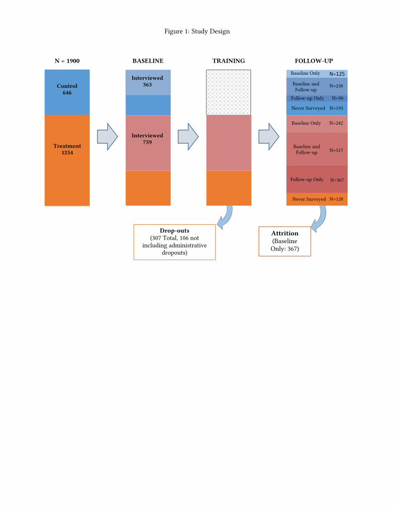
Figure 1: Study Design

 

 

 

 

Control 646

Treatment 1254

N = 1900

 

 

 

BASELINE

 

TRAINING

Drop-outs (307 Total, 106 not

including administrative dropouts)

 

FOLLOW-UP

 

 

   Interviewed

759

Baseline Only

 

Follow-up Only

Baseline and Follow-up

Never Surveyed

  Interviewed

363 Baseline and Follow-up

Follow-up Only

Never Surveyed

Attrition (Baseline

Only: 367)

Baseline Only N=125

N=238

N=90

N=193

N=242

N=517

N=367

N=128

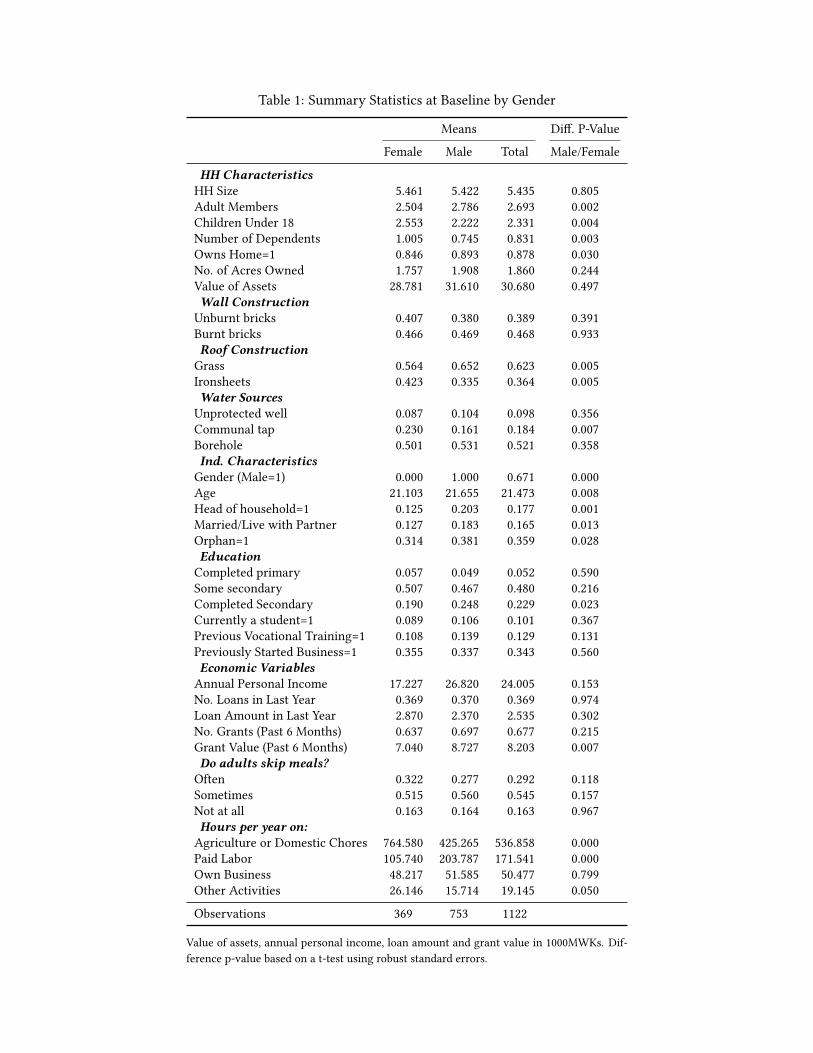
Table 1: Summary Statistics at Baseline by Gender

Means Di�. P-Value

Female Male Total Male/Female

HH CharacteristicsHH Size 5.461 5.422 5.435 0.805Adult Members 2.504 2.786 2.693 0.002Children Under 18 2.553 2.222 2.331 0.004Number of Dependents 1.005 0.745 0.831 0.003Owns Home=1 0.846 0.893 0.878 0.030No. of Acres Owned 1.757 1.908 1.860 0.244Value of Assets 28.781 31.610 30.680 0.497Wall Construction

Unburnt bricks 0.407 0.380 0.389 0.391Burnt bricks 0.466 0.469 0.468 0.933Roof Construction

Grass 0.564 0.652 0.623 0.005Ironsheets 0.423 0.335 0.364 0.005Water Sources

Unprotected well 0.087 0.104 0.098 0.356Communal tap 0.230 0.161 0.184 0.007Borehole 0.501 0.531 0.521 0.358Ind. Characteristics

Gender (Male=1) 0.000 1.000 0.671 0.000Age 21.103 21.655 21.473 0.008Head of household=1 0.125 0.203 0.177 0.001Married/Live with Partner 0.127 0.183 0.165 0.013Orphan=1 0.314 0.381 0.359 0.028Education

Completed primary 0.057 0.049 0.052 0.590Some secondary 0.507 0.467 0.480 0.216Completed Secondary 0.190 0.248 0.229 0.023Currently a student=1 0.089 0.106 0.101 0.367Previous Vocational Training=1 0.108 0.139 0.129 0.131Previously Started Business=1 0.355 0.337 0.343 0.560Economic Variables

Annual Personal Income 17.227 26.820 24.005 0.153No. Loans in Last Year 0.369 0.370 0.369 0.974Loan Amount in Last Year 2.870 2.370 2.535 0.302No. Grants (Past 6 Months) 0.637 0.697 0.677 0.215Grant Value (Past 6 Months) 7.040 8.727 8.203 0.007Do adults skip meals?

Often 0.322 0.277 0.292 0.118Sometimes 0.515 0.560 0.545 0.157Not at all 0.163 0.164 0.163 0.967Hours per year on:

Agriculture or Domestic Chores 764.580 425.265 536.858 0.000Paid Labor 105.740 203.787 171.541 0.000Own Business 48.217 51.585 50.477 0.799Other Activities 26.146 15.714 19.145 0.050

Observations 369 753 1122

Value of assets, annual personal income, loan amount and grant value in 1000MWKs. Dif-ference p-value based on a t-test using robust standard errors.

Table 2: Summary Statistics at Endline by Gender

Means Di�. P-Value

Female Male Total Male/Female

HH CharacteristicsHousehold size 4.881 4.932 4.914 0.703No. Adults 2.665 2.855 2.786 0.019No. Children Under 18 2.114 1.974 2.025 0.170Number of Dependents 1.231 1.870 1.638 0.000Owns home=1 0.772 0.880 0.841 0.000No. of Acres Owned 1.393 1.385 1.388 0.937Value of Assets 27.854 31.613 30.250 0.219Individual Characteristics

Gender:Male=1 0.000 1.000 0.637Age 21.358 22.065 21.808 0.001Head of Household=1 0.134 0.302 0.241 0.000Married or living with partner=1 0.255 0.240 0.246 0.587Orphan=1 0.363 0.449 0.418 0.005Education

All primary 0.056 0.046 0.049 0.450Some secondary 0.608 0.526 0.556 0.007All secondary 0.097 0.171 0.144 0.000Currently a student=1 0.092 0.098 0.096 0.756Received vocational training=1 0.044 0.093 0.075 0.001Addtl. simultaneous vocational training=1 0.017 0.040 0.032 0.017Economic Variables

Previously started a business=1 0.360 0.317 0.332 0.140Worked for wage in past 12 months=1 0.153 0.186 0.174 0.143Personal Savings 1.549 1.080 1.250 0.409No. Loans in Last Year 0.337 0.409 0.383 0.039Loan Amount in Last Year 3.112 2.661 2.805 0.404Prop. of Expenditure on Food 0.430 0.479 0.462 0.013Anyone in HH Skip Meals?

No 0.486 0.473 0.478 0.692Yes, but infrequently 0.306 0.326 0.319 0.536Yes, about once a month 0.096 0.088 0.090 0.663Yes, more than once month 0.111 0.114 0.113 0.904Migration

Migration Episodes in Last Year 0.221 0.218 0.219 0.926Avg. Duration of Migration Episode 7.549 8.475 8.158 0.662No. of Migration Episodes for Work Last Year 0.015 0.068 0.048 0.000Trainee Experience

Months of Training 2.884 2.907 2.898 0.654No Missed Training Days 0.479 0.530 0.511 0.238Stipend Amount Per Month 2.132 2.028 2.065 0.472Sometime Stipend was Insu�cent to Cover Needs 0.505 0.460 0.476 0.300Received Food or Money from MC 0.463 0.554 0.520 0.033MC Always Attended Training 0.819 0.811 0.814 0.795Practice Tools Always Available 0.694 0.730 0.717 0.366Felt Encouraged by MC 0.935 0.930 0.932 0.792Secured Paid Work from MC After Training 0.014 0.038 0.029 0.062

Observations 412 724 1136

Value of assets, annual personal income, loan amount and grant value in 1000MKWs. Di�erence p-valuebased on a t-test using robust standard errors. We include all households in the endline sample (i.e. thoseoriginally assigned to treatment and those who were added to the treatment after randomization) to increasestatistical power.

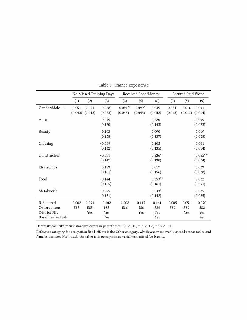
Table 3: Trainee Experience

No Missed Training Days Received Food/Money Secured Paid Work

(1) (2) (3) (4) (5) (6) (7) (8) (9)

Gender:Male=1 0.051 0.061 0.088* 0.091** 0.099** 0.039 0.024* 0.016 –0.001(0.043) (0.043) (0.053) (0.043) (0.043) (0.052) (0.013) (0.013) (0.014)

Auto –0.079 0.220 –0.009(0.150) (0.143) (0.023)

Beauty 0.103 0.090 0.019(0.158) (0.157) (0.028)

Clothing –0.039 0.105 0.001(0.142) (0.135) (0.014)

Construction –0.031 0.236* 0.065***(0.147) (0.138) (0.024)

Electronics –0.123 0.017 0.023(0.161) (0.156) (0.028)

Food –0.144 0.353** 0.022(0.165) (0.161) (0.051)

Metalwork –0.095 0.243* 0.025(0.151) (0.142) (0.025)

R-Squared 0.002 0.091 0.102 0.008 0.117 0.141 0.005 0.051 0.070Observations 585 585 585 586 586 586 582 582 582District FEs Yes Yes Yes Yes Yes YesBaseline Controls Yes Yes Yes

Heteroskedasticity-robust standard errors in parentheses. * p < .10, ** p < .05, *** p < .01.Reference category for cccupation �xed-e�ects is the Other category, which was most evenly spread across males andfemales trainees. Null results for other trainee experience variables omitted for brevity.

Table 4: Summary Statistics at Baseline: Di�erence Between Dropout andAttrition

Means Di�. P-Value

(1)DropoutsW/ AdminDropouts

(2)Dropouts

W/O AdminDropouts

(3)Attriters (1) v (3) (2) v (3)

HH CharacteristicsHH Size 5.711 5.529 5.150 0.006 0.220Adult Members 2.841 2.700 2.578 0.033 0.500Children Under 18 2.431 2.471 2.139 0.055 0.174Number of Dependents 0.612 0.643 1.060 0.000 0.008Owns Home=1 0.879 0.871 0.849 0.293 0.618No. of Acres Owned 1.903 2.167 1.868 0.895 0.662Value of Assets 35.296 24.975 22.809 0.006 0.668Wall Construction

Unburnt bricks 0.379 0.343 0.401 0.604 0.356Burnt bricks 0.483 0.529 0.490 0.854 0.560Roof Construction

Grass 0.625 0.543 0.572 0.199 0.652Ironsheets 0.358 0.414 0.411 0.188 0.965Water Sources

Unprotected well 0.078 0.057 0.104 0.270 0.146Communal tap 0.164 0.186 0.213 0.129 0.593Borehole 0.539 0.629 0.500 0.356 0.044Ind. Characteristics

Gender (Male=1) 0.659 0.629 0.657 0.944 0.656Age 20.342 20.286 23.256 0.000 0.000Head of household=1 0.147 0.200 0.240 0.004 0.452Married/Live with Partner 0.164 0.129 0.204 0.208 0.095Orphan=1 0.351 0.353 0.348 0.945 0.939Education

Completed primary 0.043 0.014 0.049 0.734 0.056Some secondary 0.461 0.457 0.520 0.158 0.332Completed Secondary 0.228 0.157 0.237 0.808 0.103Currently a student=1 0.159 0.143 0.046 0.000 0.026Previous Vocational Training=1 0.147 0.114 0.123 0.408 0.842Previously Started Business=1 0.302 0.271 0.390 0.026 0.046Economic Variables

Annual Personal Income 15.918 8.796 30.203 0.042 0.001No. Loans in Last Year 0.366 0.357 0.377 0.812 0.776Loan Amount in Last Year 2.224 2.414 2.834 0.233 0.665No. Grants (Past 6 Months) 0.659 0.614 0.728 0.292 0.268Grant Value (Past 6 Months) 8.877 7.509 9.184 0.810 0.357Do adults skip meals?

Often 0.310 0.371 0.286 0.529 0.173Sometimes 0.556 0.529 0.542 0.741 0.834Not at all 0.134 0.100 0.172 0.203 0.081Hours per year on:

Agriculture or Domestic Chores 524.582 524.389 525.232 0.986 0.989Paid Labor 167.111 152.762 197.478 0.283 0.282Own Business 42.860 66.161 68.464 0.171 0.948Other Activities 9.914 8.293 19.997 0.057 0.042

Observations 232 70 367

Value of assets, annual personal income, loan amount and grant value in 1000MWKs. Di�erence p-value based on a t-test using robust standard errors.

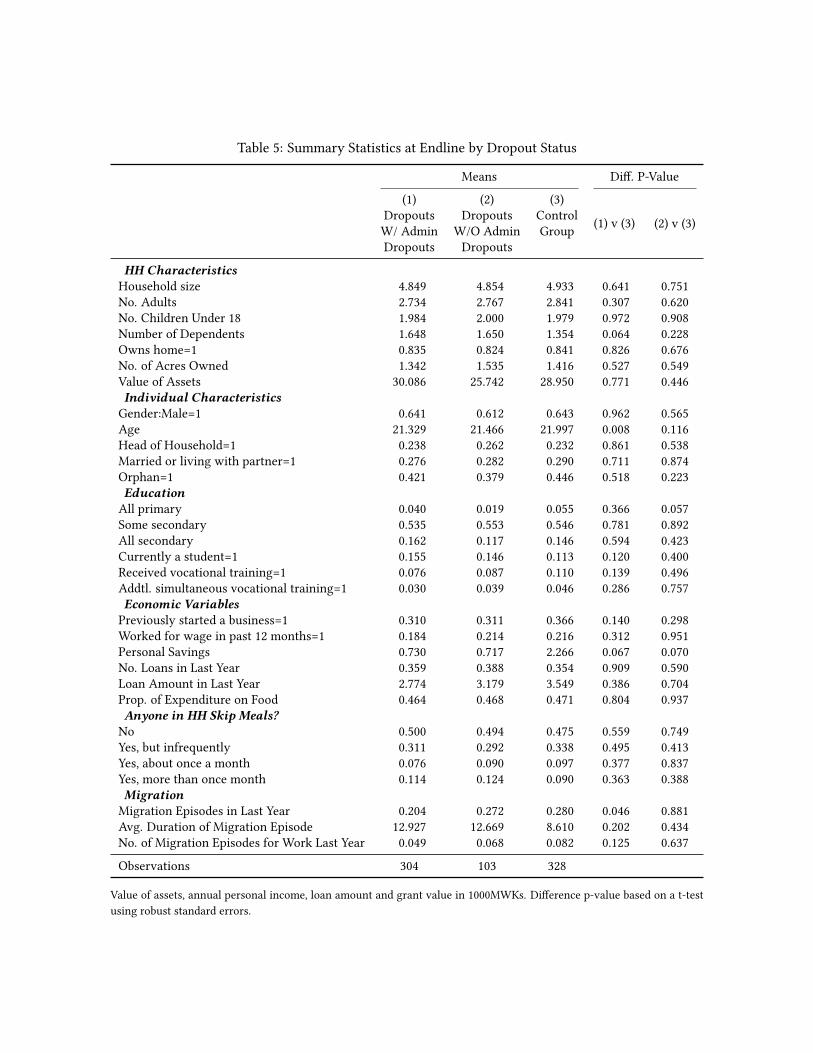
Table 5: Summary Statistics at Endline by Dropout Status

Means Di�. P-Value

(1)DropoutsW/ AdminDropouts

(2)Dropouts

W/O AdminDropouts

(3)ControlGroup (1) v (3) (2) v (3)

HH CharacteristicsHousehold size 4.849 4.854 4.933 0.641 0.751No. Adults 2.734 2.767 2.841 0.307 0.620No. Children Under 18 1.984 2.000 1.979 0.972 0.908Number of Dependents 1.648 1.650 1.354 0.064 0.228Owns home=1 0.835 0.824 0.841 0.826 0.676No. of Acres Owned 1.342 1.535 1.416 0.527 0.549Value of Assets 30.086 25.742 28.950 0.771 0.446Individual Characteristics

Gender:Male=1 0.641 0.612 0.643 0.962 0.565Age 21.329 21.466 21.997 0.008 0.116Head of Household=1 0.238 0.262 0.232 0.861 0.538Married or living with partner=1 0.276 0.282 0.290 0.711 0.874Orphan=1 0.421 0.379 0.446 0.518 0.223Education

All primary 0.040 0.019 0.055 0.366 0.057Some secondary 0.535 0.553 0.546 0.781 0.892All secondary 0.162 0.117 0.146 0.594 0.423Currently a student=1 0.155 0.146 0.113 0.120 0.400Received vocational training=1 0.076 0.087 0.110 0.139 0.496Addtl. simultaneous vocational training=1 0.030 0.039 0.046 0.286 0.757Economic Variables

Previously started a business=1 0.310 0.311 0.366 0.140 0.298Worked for wage in past 12 months=1 0.184 0.214 0.216 0.312 0.951Personal Savings 0.730 0.717 2.266 0.067 0.070No. Loans in Last Year 0.359 0.388 0.354 0.909 0.590Loan Amount in Last Year 2.774 3.179 3.549 0.386 0.704Prop. of Expenditure on Food 0.464 0.468 0.471 0.804 0.937Anyone in HH Skip Meals?

No 0.500 0.494 0.475 0.559 0.749Yes, but infrequently 0.311 0.292 0.338 0.495 0.413Yes, about once a month 0.076 0.090 0.097 0.377 0.837Yes, more than once month 0.114 0.124 0.090 0.363 0.388Migration

Migration Episodes in Last Year 0.204 0.272 0.280 0.046 0.881Avg. Duration of Migration Episode 12.927 12.669 8.610 0.202 0.434No. of Migration Episodes for Work Last Year 0.049 0.068 0.082 0.125 0.637

Observations 304 103 328

Value of assets, annual personal income, loan amount and grant value in 1000MWKs. Di�erence p-value based on a t-testusing robust standard errors.

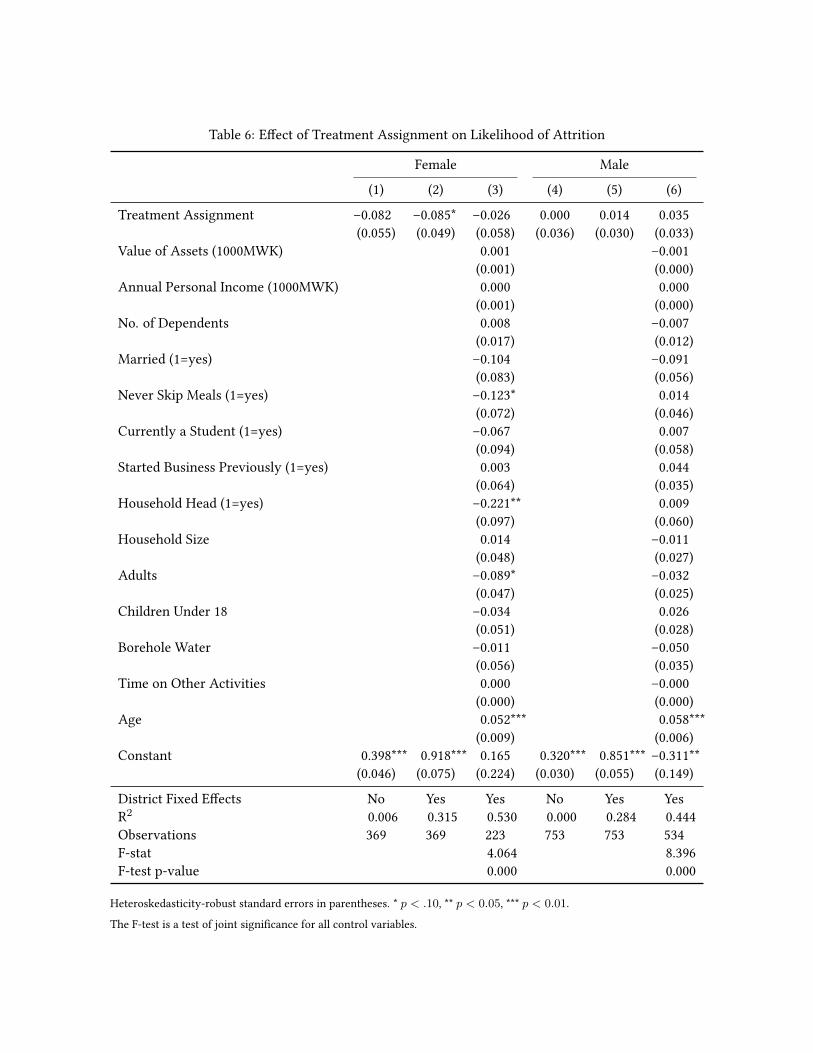
Table 6: E�ect of Treatment Assignment on Likelihood of Attrition

Female Male

(1) (2) (3) (4) (5) (6)

Treatment Assignment –0.082 –0.085* –0.026 0.000 0.014 0.035(0.055) (0.049) (0.058) (0.036) (0.030) (0.033)

Value of Assets (1000MWK) 0.001 –0.001(0.001) (0.000)

Annual Personal Income (1000MWK) 0.000 0.000(0.001) (0.000)

No. of Dependents 0.008 –0.007(0.017) (0.012)

Married (1=yes) –0.104 –0.091(0.083) (0.056)

Never Skip Meals (1=yes) –0.123* 0.014(0.072) (0.046)

Currently a Student (1=yes) –0.067 0.007(0.094) (0.058)

Started Business Previously (1=yes) 0.003 0.044(0.064) (0.035)

Household Head (1=yes) –0.221** 0.009(0.097) (0.060)

Household Size 0.014 –0.011(0.048) (0.027)

Adults –0.089* –0.032(0.047) (0.025)

Children Under 18 –0.034 0.026(0.051) (0.028)

Borehole Water –0.011 –0.050(0.056) (0.035)

Time on Other Activities 0.000 –0.000(0.000) (0.000)

Age 0.052*** 0.058***(0.009) (0.006)

Constant 0.398*** 0.918*** 0.165 0.320*** 0.851*** –0.311**(0.046) (0.075) (0.224) (0.030) (0.055) (0.149)

District Fixed E�ects No Yes Yes No Yes YesR2 0.006 0.315 0.530 0.000 0.284 0.444Observations 369 369 223 753 753 534F-stat 4.064 8.396F-test p-value 0.000 0.000

Heteroskedasticity-robust standard errors in parentheses. * p < .10, ** p < 0.05, *** p < 0.01.

The F-test is a test of joint signi�cance for all control variables.

Table 7: E�ects of Shocks on Likelihood of Dropout (OLS)

Dropped Out (W/ Admin Dropout) Dropped Out (W/O Admin. Dropout)

Female Male Di�. P-Value Female Male Di�. P-Value

Migrated (1=Yes) 0.087 0.085* 0.505 0.115 0.169*** 0.320(0.063) (0.046) (0.090) (0.057)

Lives >4KM from TC 0.106 –0.085 0.210 0.065 –0.037 0.437(0.112) (0.071) (0.137) (0.081)

Close Friends/Relatives at TC –0.570*** –0.637*** 0.384 –0.344*** –0.285*** 0.859(0.063) (0.041) (0.094) (0.070)

In Past YearFired –0.360*** 0.059 0.061 –0.409*** 0.175 0.008

(0.097) (0.109) (0.126) (0.140)Incapacitated 0.151* –0.084 0.052 0.211 –0.107 0.091

(0.088) (0.083) (0.136) (0.091)HH Member Incapacitated 0.004 0.008 0.952 –0.011 0.054 0.559

(0.056) (0.039) (0.077) (0.050)HH Member Death –0.085 –0.007 0.963 –0.104 0.012 0.797

(0.078) (0.070) (0.103) (0.085)Had Child 0.097 0.041 0.521 0.181 0.119 0.811

(0.112) (0.089) (0.153) (0.106)Married 0.086 –0.034 0.630 0.110 –0.129 0.289

(0.081) (0.070) (0.121) (0.080)Month Before TrainingHrs in Paid Labor 0.000 –0.000 0.449 0.000 –0.000 0.330

(0.000) (0.000) (0.001) (0.001)Hrs in Self Employment 0.001 –0.000 0.186 0.001 –0.000 0.181

(0.001) (0.000) (0.001) (0.000)Hrs in Skill Development 0.000 0.001* 0.743 0.001 0.001 0.768

(0.001) (0.000) (0.001) (0.001)

R-Sq 0.536 0.486 0.354 0.227Observations 225 427 157 298

Heteroskedasticity-robust standard errors in parentheses. * p < .10, ** p < 0.05, *** p < 0.01.

District and occupation �xed e�ects and controls included in each regression. Controls include: number of dependens, value of assets(1000MWKs), age and indicators for head of household, orphan status, and always being healthy. TC = training center. Sample restrictedto only those assigned to recieve treatment. Di�erence p-value based on a t-test using robust standard errors.

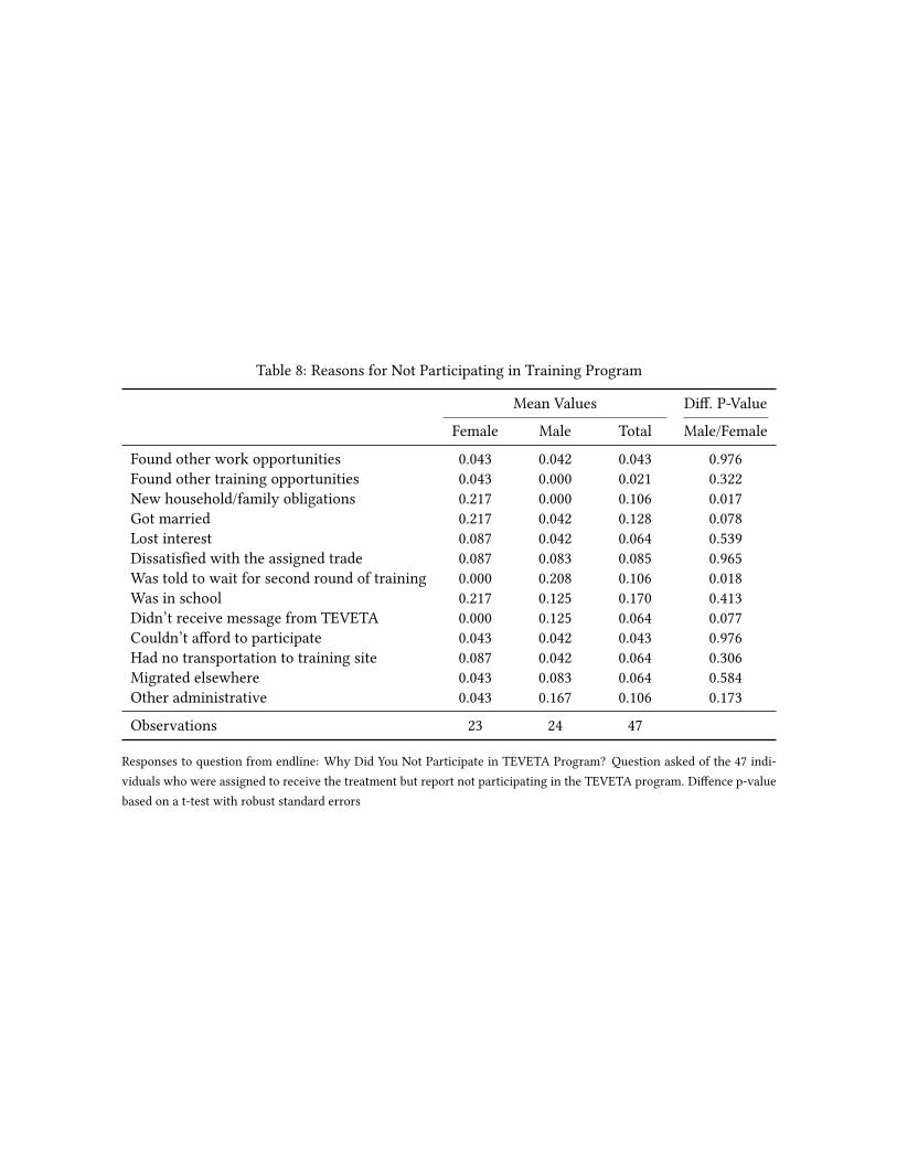
Table 8: Reasons for Not Participating in Training Program

Mean Values Di�. P-Value

Female Male Total Male/Female

Found other work opportunities 0.043 0.042 0.043 0.976Found other training opportunities 0.043 0.000 0.021 0.322New household/family obligations 0.217 0.000 0.106 0.017Got married 0.217 0.042 0.128 0.078Lost interest 0.087 0.042 0.064 0.539Dissatis�ed with the assigned trade 0.087 0.083 0.085 0.965Was told to wait for second round of training 0.000 0.208 0.106 0.018Was in school 0.217 0.125 0.170 0.413Didn’t receive message from TEVETA 0.000 0.125 0.064 0.077Couldn’t a�ord to participate 0.043 0.042 0.043 0.976Had no transportation to training site 0.087 0.042 0.064 0.306Migrated elsewhere 0.043 0.083 0.064 0.584Other administrative 0.043 0.167 0.106 0.173

Observations 23 24 47

Responses to question from endline: Why Did You Not Participate in TEVETA Program? Question asked of the 47 indi-viduals who were assigned to receive the treatment but report not participating in the TEVETA program. Di�ence p-valuebased on a t-test with robust standard errors

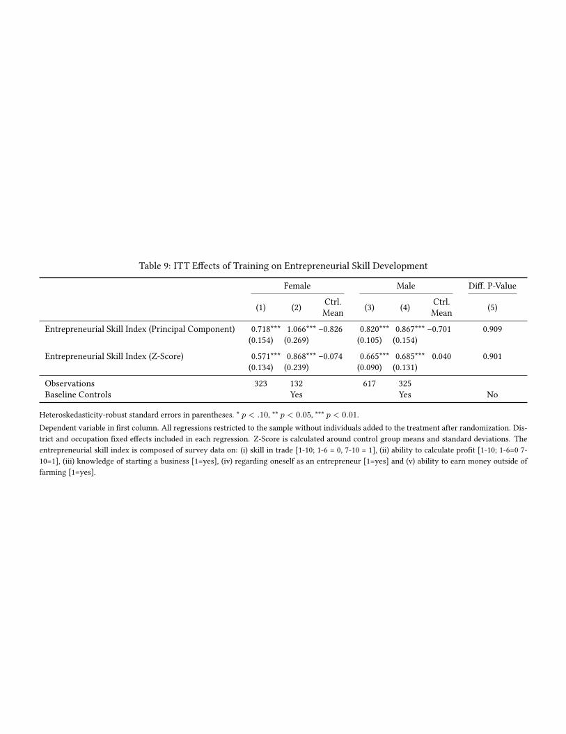
Table 9: ITT E�ects of Training on Entrepreneurial Skill Development

Female Male Di�. P-Value

(1) (2) Ctrl.Mean (3) (4) Ctrl.

Mean (5)

Entrepreneurial Skill Index (Principal Component) 0.718*** 1.066*** –0.826 0.820*** 0.867*** –0.701 0.909(0.154) (0.269) (0.105) (0.154)

Entrepreneurial Skill Index (Z-Score) 0.571*** 0.868*** –0.074 0.665*** 0.685*** 0.040 0.901(0.134) (0.239) (0.090) (0.131)

Observations 323 132 617 325Baseline Controls Yes Yes No

Heteroskedasticity-robust standard errors in parentheses. * p < .10, ** p < 0.05, *** p < 0.01.Dependent variable in �rst column. All regressions restricted to the sample without individuals added to the treatment after randomization. Dis-trict and occupation �xed e�ects included in each regression. Z-Score is calculated around control group means and standard deviations. Theentrepreneurial skill index is composed of survey data on: (i) skill in trade [1-10; 1-6 = 0, 7-10 = 1], (ii) ability to calculate pro�t [1-10; 1-6=0 7-10=1], (iii) knowledge of starting a business [1=yes], (iv) regarding oneself as an entrepreneur [1=yes] and (v) ability to earn money outside offarming [1=yes].

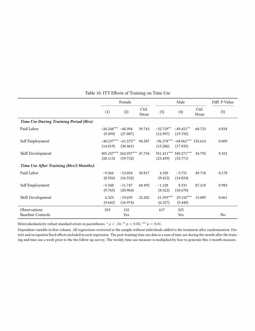
Table 10: ITT E�ects of Training on Time Use

Female Male Di�. P-Value

(1) (2) Ctrl.Mean (3) (4) Ctrl.

Mean (5)

Time Use During Training Period (Hrs):

Paid Labor –26.248*** –40.394 39.743 –32.729** –49.451** 68.723 0.834(9.499) (27.087) (12.997) (19.795)

Self Employment –40.237*** –61.575** 94.587 –96.278*** –68.061*** 155.614 0.009(14.019) (30.461) (15.286) (17.835)

Skill Development 305.237*** 262.037*** 47.734 351.411*** 349.271*** 34.792 0.321(28.113) (59.732) (23.439) (33.771)

Time Use A�er Training (Hrs/2 Months):

Paid Labor –9.266 –13.054 30.817 4.350 –3.751 49.718 0.178(8.556) (16.532) (9.412) (14.824)

Self Employment –5.348 –11.747 68.495 –1.128 8.531 87.218 0.983(9.765) (20.964) (8.322) (10.670)

Skill Development 6.325 –19.695 22.202 21.593*** 29.152*** 15.089 0.061(9.642) (16.974) (6.227) (9.440)

Observations 323 132 617 325Baseline Controls Yes Yes No

Heteroskedasticity-robust standard errors in parentheses. * p < .10, ** p < 0.05, *** p < 0.01.Dependent variable in �rst column. All regressions restricted to the sample without individuals added to the treatment after randomization. Dis-trict and occupation �xed e�ects included in each regression. The post-training time use data is a sum of time use during the month after the train-ing and time use a week prior to the the follow up survey. The weekly time use measure is multiplied by four to generate this 2-month measure.

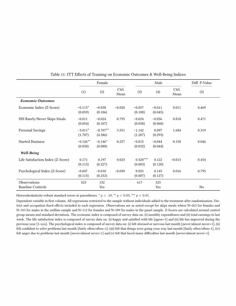
Table 11: ITT E�ects of Training on Economic Outcomes & Well-Being Indices

Female Male Di�. P-Value

(1) (2) Ctrl.Mean (3) (4) Ctrl.

Mean (5)

Economic Outcomes

Economic Index (Z-Score) –0.115* –0.058 –0.020 –0.057 –0.011 0.011 0.469(0.059) (0.106) (0.108) (0.045)

HH Rarely/Never Skips Meals –0.011 –0.024 0.795 –0.024 –0.056 0.818 0.471(0.054) (0.107) (0.038) (0.060)

Personal Savings –3.011* –8.707** 3.551 –1.142 0.097 1.684 0.319(1.707) (4.386) (1.287) (0.293)

Started Business –0.126** –0.146* 0.257 –0.015 –0.044 0.158 0.046(0.050) (0.088) (0.032) (0.044)

Well-Being

Life Satisfaction Index (Z-Score) 0.171 0.197 0.023 0.328*** 0.122 –0.013 0.454(0.113) (0.227) (0.083) (0.120)

Psychological Index (Z-Score) –0.047 –0.010 –0.030 0.025 0.145 0.016 0.795(0.115) (0.232) (0.087) (0.127)

Observations 323 132 617 325Baseline Controls Yes Yes No

Heteroskedasticity-robust standard errors in parentheses. * p < .10, ** p < 0.05, *** p < 0.01.Dependent variable in �rst column. All regressions restricted to the sample without individuals added to the treatment after randomization. Dis-trict and occupation �xed e�ects included in each regression. Observations are as noted except for skips meals where N=263 for females andN=553 for males in the endline sample and N=112 for females and N=289 for males in the panel sample. Z-Scores are calculated around controlgroup means and standard deviations. The economic index is composed of survey data on: (i) monthly expenditures and (ii) total earnings in lastweek. The life satisfaction index is composed of survey data on: (i) happy and satis�ed with life [agree=1] and (ii) life has improved during theprevious year [1=yes]. The psychological index is composed of survey data on: (i) felt stressed or nervous last month [never/almost never=1], (ii)felt con�dent to solve problems last month [fairly often/often=1], (iii) felt that things were going your way last month [fairly often/often=1], (iv)felt anger due to problems last month [never/almost never=1] and (v) felt that faced many di�culties last month [never/almost never=1].

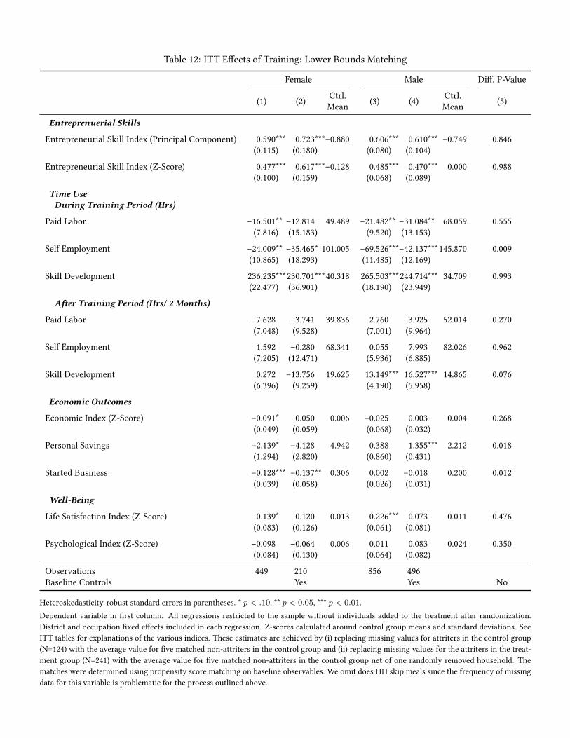
Table 12: ITT E�ects of Training: Lower Bounds Matching

Female Male Di�. P-Value

(1) (2) Ctrl.Mean (3) (4) Ctrl.

Mean (5)

Entreprenuerial Skills

Entrepreneurial Skill Index (Principal Component) 0.590*** 0.723***–0.880 0.606*** 0.610*** –0.749 0.846(0.115) (0.180) (0.080) (0.104)

Entrepreneurial Skill Index (Z-Score) 0.477*** 0.617***–0.128 0.485*** 0.470*** 0.000 0.988(0.100) (0.159) (0.068) (0.089)

Time UseDuring Training Period (Hrs)

Paid Labor –16.501** –12.814 49.489 –21.482** –31.084** 68.059 0.555(7.816) (15.183) (9.520) (13.153)

Self Employment –24.009** –35.465* 101.005 –69.526***–42.137***145.870 0.009(10.865) (18.293) (11.485) (12.169)

Skill Development 236.235***230.701***40.318 265.503***244.714*** 34.709 0.993(22.477) (36.901) (18.190) (23.949)

A�er Training Period (Hrs/ 2 Months)

Paid Labor –7.628 –3.741 39.836 2.760 –3.925 52.014 0.270(7.048) (9.528) (7.001) (9.964)

Self Employment 1.592 –0.280 68.341 0.055 7.993 82.026 0.962(7.205) (12.471) (5.936) (6.885)

Skill Development 0.272 –13.756 19.625 13.149*** 16.527*** 14.865 0.076(6.396) (9.259) (4.190) (5.958)

Economic Outcomes

Economic Index (Z-Score) –0.091* 0.050 0.006 –0.025 0.003 0.004 0.268(0.049) (0.059) (0.068) (0.032)

Personal Savings –2.139* –4.128 4.942 0.388 1.355*** 2.212 0.018(1.294) (2.820) (0.860) (0.431)

Started Business –0.128*** –0.137** 0.306 0.002 –0.018 0.200 0.012(0.039) (0.058) (0.026) (0.031)

Well-Being

Life Satisfaction Index (Z-Score) 0.139* 0.120 0.013 0.226*** 0.073 0.011 0.476(0.083) (0.126) (0.061) (0.081)

Psychological Index (Z-Score) –0.098 –0.064 0.006 0.011 0.083 0.024 0.350(0.084) (0.130) (0.064) (0.082)

Observations 449 210 856 496Baseline Controls Yes Yes No

Heteroskedasticity-robust standard errors in parentheses. * p < .10, ** p < 0.05, *** p < 0.01.Dependent variable in �rst column. All regressions restricted to the sample without individuals added to the treatment after randomization.District and occupation �xed e�ects included in each regression. Z-scores calculated around control group means and standard deviations. SeeITT tables for explanations of the various indices. These estimates are achieved by (i) replacing missing values for attriters in the control group(N=124) with the average value for �ve matched non-attriters in the control group and (ii) replacing missing values for the attriters in the treat-ment group (N=241) with the average value for �ve matched non-attriters in the control group net of one randomly removed household. Thematches were determined using propensity score matching on baseline observables. We omit does HH skip meals since the frequency of missingdata for this variable is problematic for the process outlined above.

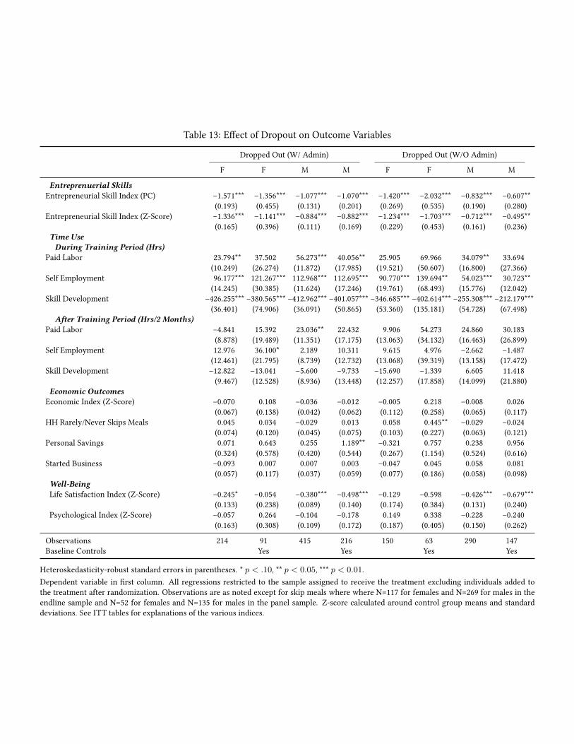
Table 13: E�ect of Dropout on Outcome Variables

Dropped Out (W/ Admin) Dropped Out (W/O Admin)

F F M M F F M M

Entreprenuerial SkillsEntrepreneurial Skill Index (PC) –1.571*** –1.356*** –1.077*** –1.070*** –1.420*** –2.032*** –0.832*** –0.607**

(0.193) (0.455) (0.131) (0.201) (0.269) (0.535) (0.190) (0.280)Entrepreneurial Skill Index (Z-Score) –1.336*** –1.141*** –0.884*** –0.882*** –1.234*** –1.703*** –0.712*** –0.495**

(0.165) (0.396) (0.111) (0.169) (0.229) (0.453) (0.161) (0.236)Time UseDuring Training Period (Hrs)

Paid Labor 23.794** 37.502 56.273*** 40.056** 25.905 69.966 34.079** 33.694(10.249) (26.274) (11.872) (17.985) (19.521) (50.607) (16.800) (27.366)

Self Employment 96.177*** 121.267*** 112.968*** 112.695*** 90.770*** 139.694** 54.023*** 30.723**(14.245) (30.385) (11.624) (17.246) (19.761) (68.493) (15.776) (12.042)

Skill Development –426.255*** –380.565*** –412.962*** –401.057*** –346.685*** –402.614*** –255.308*** –212.179***(36.401) (74.906) (36.091) (50.865) (53.360) (135.181) (54.728) (67.498)

A�er Training Period (Hrs/2 Months)Paid Labor –4.841 15.392 23.036** 22.432 9.906 54.273 24.860 30.183

(8.878) (19.489) (11.351) (17.175) (13.063) (34.132) (16.463) (26.899)Self Employment 12.976 36.100* 2.189 10.311 9.615 4.976 –2.662 –1.487

(12.461) (21.795) (8.739) (12.732) (13.068) (39.319) (13.158) (17.472)Skill Development –12.822 –13.041 –5.600 –9.733 –15.690 –1.339 6.605 11.418

(9.467) (12.528) (8.936) (13.448) (12.257) (17.858) (14.099) (21.880)Economic Outcomes

Economic Index (Z-Score) –0.070 0.108 –0.036 –0.012 –0.005 0.218 –0.008 0.026(0.067) (0.138) (0.042) (0.062) (0.112) (0.258) (0.065) (0.117)

HH Rarely/Never Skips Meals 0.045 0.034 –0.029 0.013 0.058 0.445** –0.029 –0.024(0.074) (0.120) (0.045) (0.075) (0.103) (0.227) (0.063) (0.121)

Personal Savings 0.071 0.643 0.255 1.189** –0.321 0.757 0.238 0.956(0.324) (0.578) (0.420) (0.544) (0.267) (1.154) (0.524) (0.616)

Started Business –0.093 0.007 0.007 0.003 –0.047 0.045 0.058 0.081(0.057) (0.117) (0.037) (0.059) (0.077) (0.186) (0.058) (0.098)

Well-BeingLife Satisfaction Index (Z-Score) –0.245* –0.054 –0.380*** –0.498*** –0.129 –0.598 –0.426*** –0.679***

(0.133) (0.238) (0.089) (0.140) (0.174) (0.384) (0.131) (0.240)Psychological Index (Z-Score) –0.057 0.264 –0.104 –0.178 0.149 0.338 –0.228 –0.240

(0.163) (0.308) (0.109) (0.172) (0.187) (0.405) (0.150) (0.262)

Observations 214 91 415 216 150 63 290 147Baseline Controls Yes Yes Yes Yes

Heteroskedasticity-robust standard errors in parentheses. * p < .10, ** p < 0.05, *** p < 0.01.Dependent variable in �rst column. All regressions restricted to the sample assigned to receive the treatment excluding individuals added tothe treatment after randomization. Observations are as noted except for skip meals where where N=117 for females and N=269 for males in theendline sample and N=52 for females and N=135 for males in the panel sample. Z-score calculated around control group means and standarddeviations. See ITT tables for explanations of the various indices.

Appendix for Online Publication Only

Gender Differences in the Effects of Vocational

Training: Constraints on Women and Dropout

Behavior

Yoonyoung Cho, World Bank

Davie Kalomba, Malawi National AIDS Commission

Ahmed Mush�q Mobarak, Yale University

Victor Orozco, World Bank

Derek Wolfson, UC Berkeley

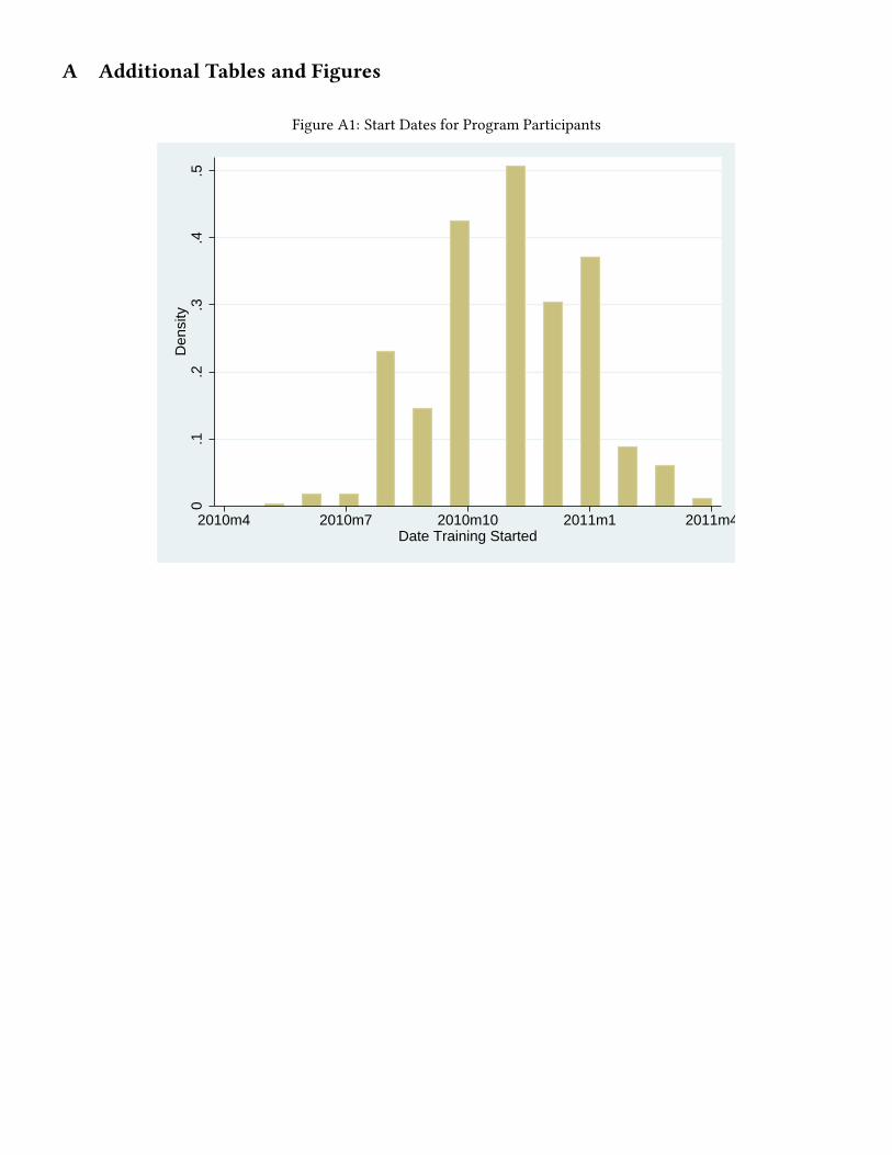
A Additional Tables and Figures

Figure A1: Start Dates for Program Participants

0.1

.2.3

.4.5

Den

sity

2010m4 2010m7 2010m10 2011m1 2011m4Date Training Started

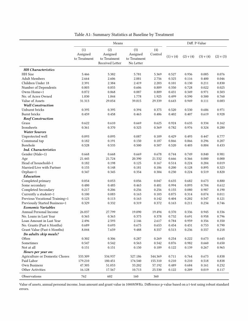
Table A1: Summary Statistics at Baseline by Treatment

Means Di�. P-Value

(1)

Assigned

to Treatment

(2)

Assigned

to Treatment

Received Letter

(3)

Assigned

to Treatment

No Letter

(4)

Control

(1) v (4) (2) v (4) (3) v (4) (2) v (3)

HH CharacteristicsHH Size 5.466 5.382 5.781 5.369 0.527 0.936 0.085 0.076

Adult Members 2.664 2.606 2.881 2.756 0.325 0.116 0.400 0.046

Children Under 18 2.391 2.384 2.419 2.203 0.101 0.130 0.211 0.830

Number of Dependents 0.803 0.855 0.606 0.889 0.350 0.728 0.022 0.025

Owns Home=1 0.872 0.868 0.887 0.889 0.431 0.349 0.971 0.503

No. of Acres Owned 1.830 1.844 1.778 1.925 0.499 0.590 0.500 0.760

Value of Assets 31.313 29.054 39.815 29.339 0.643 0.949 0.111 0.083

Wall ConstructionUnburnt bricks 0.395 0.395 0.394 0.375 0.520 0.530 0.686 0.971

Burnt bricks 0.459 0.458 0.463 0.486 0.402 0.407 0.619 0.928

Roof ConstructionGrass 0.622 0.610 0.669 0.625 0.924 0.635 0.334 0.162

Ironsheets 0.361 0.370 0.325 0.369 0.782 0.976 0.324 0.280

Water SourcesUnprotected well 0.093 0.095 0.087 0.109 0.429 0.493 0.447 0.777

Communal tap 0.182 0.191 0.150 0.187 0.866 0.866 0.296 0.207

Borehole 0.528 0.535 0.500 0.507 0.520 0.403 0.884 0.433

Ind. CharacteristicsGender (Male=1) 0.668 0.668 0.669 0.678 0.744 0.749 0.840 0.981

Age 21.445 21.724 20.390 21.532 0.666 0.366 0.000 0.000

Head of household=1 0.182 0.198 0.125 0.167 0.514 0.224 0.204 0.019

Married/Live with Partner 0.155 0.148 0.181 0.186 0.200 0.128 0.895 0.323

Orphan=1 0.347 0.345 0.354 0.384 0.230 0.224 0.519 0.820

EducationCompleted primary 0.054 0.053 0.056 0.047 0.635 0.682 0.673 0.880

Some secondary 0.480 0.485 0.463 0.481 0.994 0.893 0.704 0.612

Completed Secondary 0.217 0.206 0.256 0.256 0.155 0.080 0.987 0.190

Currently a student=1 0.100 0.083 0.163 0.103 0.875 0.314 0.074 0.011

Previous Vocational Training=1 0.123 0.113 0.163 0.142 0.404 0.202 0.547 0.121

Previously Started Business=1 0.329 0.332 0.319 0.372 0.163 0.211 0.234 0.746

Economic VariablesAnnual Personal Income 26.037 27.799 19.090 19.494 0.370 0.336 0.945 0.336

No. Loans in Last Year 0.365 0.363 0.375 0.378 0.732 0.691 0.958 0.796

Loan Amount in Last Year 2.496 2.593 2.146 2.617 0.784 0.959 0.356 0.350

No. Grants (Past 6 Months) 0.689 0.693 0.675 0.653 0.454 0.431 0.753 0.790

Grant Value (Past 6 Months) 8.044 7.659 9.488 8.557 0.513 0.236 0.557 0.218

Do adults skip meals?Often 0.302 0.306 0.287 0.269 0.254 0.222 0.673 0.645

Sometimes 0.547 0.542 0.563 0.542 0.876 0.982 0.660 0.650

Not at all 0.151 0.151 0.150 0.189 0.122 0.139 0.267 0.965

Hours per year on:Agriculture or Domestic Chores 533.309 534.937 527.186 544.369 0.711 0.764 0.673 0.838

Paid Labor 179.210 180.451 174.540 155.310 0.210 0.210 0.518 0.838

Own Business 47.305 51.053 33.202 57.192 0.489 0.684 0.161 0.232

Other Activities 16.128 17.567 10.713 25.530 0.122 0.209 0.019 0.117

Observations 762 602 160 360

Value of assets, annual personal income, loan amount and grant value in 1000MWKs. Di�erence p-value based on a t-test using robust standard

errors.

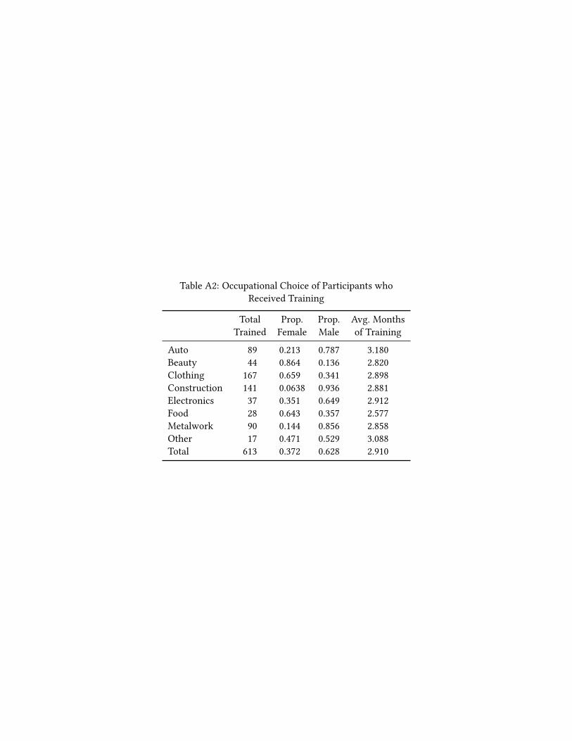
Table A2: Occupational Choice of Participants who

Received Training

Total

Trained

Prop.

Female

Prop.

Male

Avg. Months

of Training

Auto 89 0.213 0.787 3.180

Beauty 44 0.864 0.136 2.820

Clothing 167 0.659 0.341 2.898

Construction 141 0.0638 0.936 2.881

Electronics 37 0.351 0.649 2.912

Food 28 0.643 0.357 2.577

Metalwork 90 0.144 0.856 2.858

Other 17 0.471 0.529 3.088

Total 613 0.372 0.628 2.910

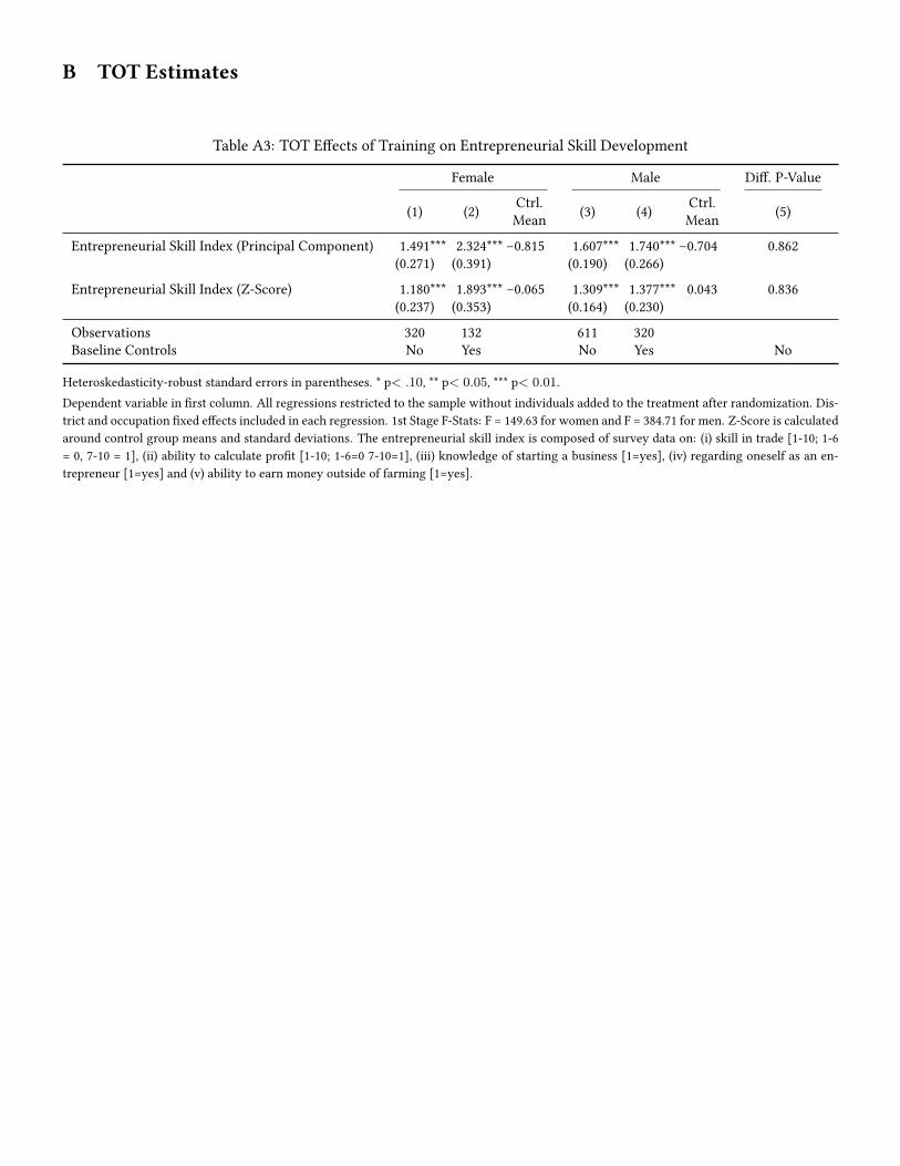
B TOT Estimates

Table A3: TOT E�ects of Training on Entrepreneurial Skill Development

Female Male Di�. P-Value

(1) (2)

Ctrl.

Mean

(3) (4)

Ctrl.

Mean

(5)

Entrepreneurial Skill Index (Principal Component) 1.491*** 2.324*** –0.815 1.607*** 1.740*** –0.704 0.862

(0.271) (0.391) (0.190) (0.266)

Entrepreneurial Skill Index (Z-Score) 1.180*** 1.893*** –0.065 1.309*** 1.377*** 0.043 0.836

(0.237) (0.353) (0.164) (0.230)

Observations 320 132 611 320

Baseline Controls No Yes No Yes No

Heteroskedasticity-robust standard errors in parentheses. * p< .10, ** p< 0.05, *** p< 0.01.

Dependent variable in �rst column. All regressions restricted to the sample without individuals added to the treatment after randomization. Dis-

trict and occupation �xed e�ects included in each regression. 1st Stage F-Stats: F = 149.63 for women and F = 384.71 for men. Z-Score is calculated

around control group means and standard deviations. The entrepreneurial skill index is composed of survey data on: (i) skill in trade [1-10; 1-6

= 0, 7-10 = 1], (ii) ability to calculate pro�t [1-10; 1-6=0 7-10=1], (iii) knowledge of starting a business [1=yes], (iv) regarding oneself as an en-

trepreneur [1=yes] and (v) ability to earn money outside of farming [1=yes].

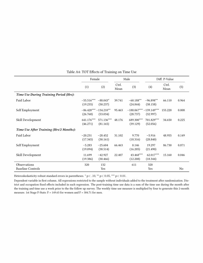
Table A4: TOT E�ects of Training on Time Use

Female Male Di�. P-Value

(1) (2)

Ctrl.

Mean

(3) (4)

Ctrl.

Mean

(5)

Time Use During Training Period (Hrs):

Paid Labor –55.516*** –88.043* 39.741 –60.188** –96.898** 66.110 0.964

(19.235) (50.237) (24.844) (38.158)

Self Employment –86.420*** –134.210** 95.463 –188.067*** –139.149*** 155.220 0.008

(26.768) (53.034) (28.737) (32.997)

Skill Development 641.176*** 571.136*** 48.176 689.300*** 701.829*** 34.650 0.225

(46.271) (81.165) (39.129) (52.056)

Time Use A�er Training (Hrs/2 Months):

Paid Labor –20.231 –28.452 31.102 9.770 –5.916 48.955 0.149

(17.345) (30.161) (18.316) (28.840)

Self Employment –5.283 –25.604 66.463 0.146 19.297 86.730 0.871

(19.094) (38.514) (16.205) (21.490)

Skill Development 11.699 –42.927 22.407 43.468*** 62.017*** 15.160 0.046

(19.386) (30.466) (12.208) (18.344)

Observations 320 132 611 320

Baseline Controls Yes Yes No

Heteroskedasticity-robust standard errors in parentheses. * p< .10, ** p< 0.05, *** p< 0.01.

Dependent variable in �rst column. All regressions restricted to the sample without individuals added to the treatment after randomization. Dis-

trict and occupation �xed e�ects included in each regression. The post-training time use data is a sum of the time use during the month after

the training and time use a week prior to the the follow up survey. The weekly time use measure is multiplied by four to generate this 2-month

measure. 1st Stage F-Stats: F = 149.63 for women and F = 384.71 for men.

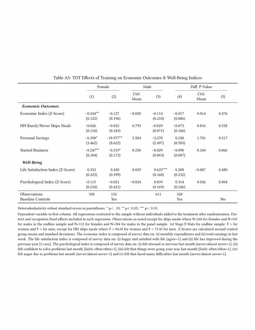
Table A5: TOT E�ects of Training on Economic Outcomes & Well-Being Indices

Female Male Di�. P-Value

(1) (2)

Ctrl.

Mean

(3) (4)

Ctrl.

Mean

(5)

Economic Outcomes

Economic Index (Z-Score) –0.244** –0.127 –0.020 –0.114 –0.017 0.014 0.476

(0.122) (0.196) (0.210) (0.086)

HH Rarely/Never Skips Meals –0.026 –0.052 0.793 –0.029 –0.073 0.816 0.558

(0.110) (0.183) (0.071) (0.106)

Personal Savings –6.390* –18.977** 3.584 –2.270 0.230 1.701 0.317

(3.462) (8.622) (2.497) (0.585)

Started Business –0.247** –0.319* 0.250 –0.029 –0.090 0.160 0.066

(0.104) (0.172) (0.063) (0.087)

Well-Being

Life Satisfaction Index (Z-Score) 0.352 0.430 0.029 0.625*** 0.208 –0.007 0.480

(0.225) (0.399) (0.160) (0.232)

Psychological Index (Z-Score) –0.115 –0.021 –0.024 0.039 0.314 0.026 0.804

(0.234) (0.421) (0.169) (0.246)

Observations 320 132 611 320

Baseline Controls Yes Yes No

Heteroskedasticity-robust standard errors in parentheses. * p< .10, ** p< 0.05, *** p< 0.01.

Dependent variable in �rst column. All regressions restricted to the sample without individuals added to the treatment after randomization. Dis-

trict and occupation �xed e�ects included in each regression. Observations as noted except for skips meals where N=260 for females and N=547

for males in the endline sample and N=112 for females and N=284 for males in the panel sample. 1st Stage F-Stats for endline sample: F = for

women and F = for men, except for HH skips meals where F = 84.05 for women and F = 73.45 for men. Z-Scores are calculated around control

group means and standard deviations. The economic index is composed of survey data on: (i) monthly expenditures and (ii) total earnings in last

week. The life satisfaction index is composed of survey data on: (i) happy and satis�ed with life [agree=1] and (ii) life has improved during the

previous year [1=yes]. The psychological index is composed of survey data on: (i) felt stressed or nervous last month [never/almost never=1], (ii)

felt con�dent to solve problems last month [fairly often/often=1], (iii) felt that things were going your way last month [fairly often/often=1], (iv)

felt anger due to problems last month [never/almost never=1] and (v) felt that faced many di�culties last month [never/almost never=1].

C Robustness to MC-Related Controls

In addition to the speci�cations in the main paper, we conduct analysis controlling for MC-related controls. In this

section, we include controls for the number of trainees in the group, the number of years the MC has been in their trade

and if the MC and trainee are the same gender. As an additional note, since those in the control group did not participate

in training we imputed zeros in all of these categories for all control group members. As such, the coe�cient estimates

associated the MC-related control variables represent interaction e�ects with the treatment assignment.

Trainees were trained by individuals with an average of 15 years of experience in groups of 4-5, on average. About

74% of trainees were the same gender as their MC, with large di�erences across gender: 24% of women were trained by

female MCs and 96% of men were trained by male MCs. This last result suggests that the variable we use to encode if

the gender of the trainee matches the gender of the MC for males is highly collinear with our treatment variable, which

may reduce the precision of the following estimates for males.

We do not have data on every MC, meaning these results come from systematically smaller samples than the main

results. Before testing the robustness of our estimates to the inclusion of MC-related controls, we �rst ensure the results

from the main paper are mirrored with smaller samples. In Tables A6-A8, we run the most parsimonious speci�cation

on the reduced samples in columns (1) and (3) and then include MC-related controls in columns (2) and (4) as robustness

checks.

C.1 Entrepreneurial Skill Development

In the smaller sample we again identify the main results we present in the paper from Table 9 (i.e. strong positive

increases in self-reported entrepreneurial skills). We also �nd that these results are robust to the inclusion of MC-related

controls (see Table A6). For women, we �nd that self-reported entrepreneurial skills may be an increasing function of

group size, suggesting the presence of peer e�ects. In all other cases, the MC-related controls are indistinguishable from

zero, suggesting that the remainder of the MC-related controls are inconsequential in these speci�cation.

C.2 Time Use

The parsimonious speci�cation in Table A7 mirrors the results from the main analysis sample in Table 10. We �nd that

most of our results for time use during the training period are robust to the inclusion of MC-related controls. However,

time in skill development during the training period for males seems to be partially explained by trainees who were

matched with Male MCs (see column (4) of A7).

For time use after training, the parsimonious speci�cation again matches the results highlighted in Table 10. For

females, we �nd the coe�cient estimates on the treatment variable including MC-related controls are stable. However,

we do �nd evidence that females in larger groups are less likely to spend time in paid labor after the training and

women who are trained by female MCs are less likely to continue skill development after the conclusion of the training.

Further, a primary result that we highlight in the paper is that male trainees spend more time in skill development

after the training period is over, however, these results are not robust to the inclusion of MC-related controls. Notably,

it seems that having a gender match between the MC and the trainee is important for this post-treatment behavioral

response. Nevertheless, we must note the collinearity between this gender match variable and the treatment assignment

for men, which make it di�cult to identify the treatment and gender match e�ects separately.

C.3 Economic Outcomes and Well-Being Indices

The results on economic outcomes and well-being presented in Table 11 in the main paper are recast with MC-related

controls in Table A8. In the parsimonious model, we no longer �nd that women reduce their personal savings to

participate in the program or are less likely to start a business after the programs completion. These results suggest

that this reduced sample cannot be used to test the robustness of these results to MC-related controls since we cannot

separately identify robustness from sample selection. Using this reduced sample we also �nd that women assigned to

treatment are more likely to have a higher life satisfaction index, although this is partially o�set by larger group sizes.

The single result that is identi�ed through the parsimonious speci�cation in this section and the main speci�cation in

Table 11 is positive and signi�cant improvements in the life satisfaction index for men. However, the evidence in table

A8 suggests this estimated e�ect is not robust to the inclusion of MC-related controls.

Table A6: ITT E�ects of Training on Entrepreneurial Skill Development with Additonal MC-related Controls

Female Male

(1) (2)

Ctrl.

Mean

(3) (4)

Ctrl.

Mean

Entrepreneurial Skill Index (Principal Component) 1.546*** 1.354*** –0.825 1.290*** 1.547*** –0.708

(0.173) (0.360) (0.119) (0.365)

No. of Trainees in Group 0.070** 0.028

(0.035) (0.037)

MC Years in Trade –0.009 –0.005

(0.015) (0.010)

MC Gender = Trainee Gender –0.016 –0.306

(0.366) (0.345)

Entrepreneurial Skill Index (Z-Score) 1.273*** 1.206*** –0.074 1.056*** 1.351*** 0.040

(0.149) (0.300) (0.100) (0.296)

No. of Trainees in Group 0.053* 0.019

(0.028) (0.031)

MC Years in Trade –0.012 –0.003

(0.013) (0.008)

MC Gender = Trainee Gender –0.045 –0.329

(0.309) (0.276)

Observations 203 203 411 411

Heteroskedasticity-robust standard errors in parentheses. * p < .10, ** p < .05, *** p < .01.

Dependent variable are the unindented entries in the �rst column. The MC-related controls are included in each regression and are the indented

entries in the �rst column. All regressions restricted to the sample without individuals added to the treatment after randomization. District �xed

e�ects included in each regression. Z-Score is calculated around control group means and standard deviations. The entrepreneurial skill index is

composed of survey data on: (i) skill in trade [1-10; 1-6 = 0, 7-10 = 1], (ii) ability to calculate pro�t [1-10; 1-6=0 7-10=1], (iii) knowledge of starting

a business [1=yes], (iv) regarding oneself as an entrepreneur [1=yes] and (v) ability to earn money outside of farming [1=yes].

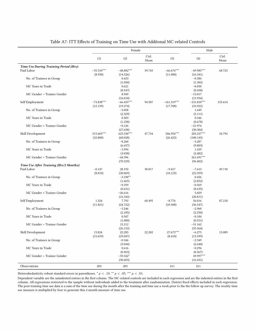
Table A7: ITT E�ects of Training on Time Use with Additonal MC-related Controls

Female Male

(1) (2)

Ctrl.

Mean

(3) (4)

Ctrl.

Mean

Time Use During Training Period (Hrs):Paid Labor –35.310*** –48.802*** 39.743 –66.674*** –49.985*** 68.723

(8.930) (14.526) (11.080) (16.341)

No. of Trainees in Group 0.423 –0.386

(1.050) (1.302)

MC Years in Trade 0.621 –0.030

(0.547) (0.438)

MC Gender = Trainee Gender 8.949 –15.017

(16.010) (15.934)

Self Employment –73.838*** –66.455*** 94.587 –161.319*** –151.810*** 155.614

(12.139) (19.274) (17.708) (33.922)

No. of Trainees in Group –3.058 1.649

(2.329) (2.111)

MC Years in Trade 0.503 0.346

(1.258) (0.678)

MC Gender = Trainee Gender –0.126 –21.974

(27.638) (30.384)

Skill Development 515.603*** 625.530*** 47.734 546.954*** 283.237*** 34.792

(32.800) (60.028) (26.423) (100.145)

No. of Trainees in Group –8.260 –3.287

(6.657) (9.803)

MC Years in Trade –3.994 1.439

(3.038) (2.482)

MC Gender = Trainee Gender –44.396 261.691***

(70.529) (96.402)

Time Use A�er Training (Hrs/2 Months):Paid Labor –0.147 28.192 30.817 –9.417 –7.615 49.718

(8.810) (20.069) (10.123) (22.359)

No. of Trainees in Group –3.330** 0.456

(1.665) (2.852)

MC Years in Trade –0.359 –0.569

(0.631) (0.635)

MC Gender = Trainee Gender –26.616 5.029

(16.342) (20.811)

Self Employment 1.324 7.792 68.495 –8.774 56.016 87.218

(11.821) (24.722) (10.308) (36.547)

No. of Trainees in Group –3.246 –2.960

(2.185) (2.250)

MC Years in Trade 0.347 –0.184

(1.000) (0.551)

MC Gender = Trainee Gender 15.212 –51.162

(26.152) (35.564)

Skill Development 13.824 22.285 22.202 27.673*** –6.275 15.089

(15.659) (29.047) (8.410) (13.599)

No. of Trainees in Group –0.346 –2.549

(3.044) (2.640)

MC Years in Trade 0.616 –0.296

(0.963) (0.567)

MC Gender = Trainee Gender –59.322* 49.997***

(30.603) (16.431)

Observations 203 203 411 411

Heteroskedasticity-robust standard errors in parentheses. * p < .10, ** p < .05, *** p < .01.

Dependent variable are the unindented entries in the �rst column. The MC-related controls are included in each regression and are the indented entries in the �rst

column. All regressions restricted to the sample without individuals added to the treatment after randomization. District �xed e�ects included in each regression.

The post-training time use data is a sum of the time use during the month after the training and time use a week prior to the the follow up survey. The weekly time

use measure is multiplied by four to generate this 2-month measure of time use.

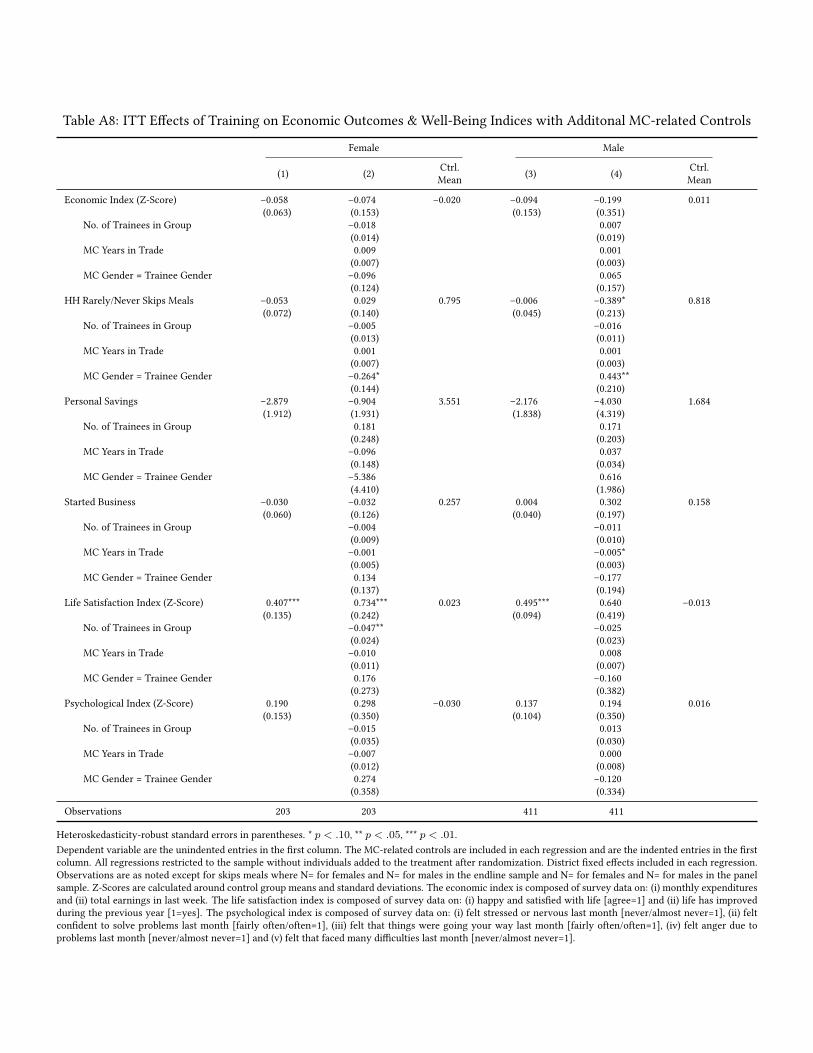
Table A8: ITT E�ects of Training on Economic Outcomes & Well-Being Indices with Additonal MC-related Controls

Female Male

(1) (2)

Ctrl.

Mean

(3) (4)

Ctrl.

Mean

Economic Index (Z-Score) –0.058 –0.074 –0.020 –0.094 –0.199 0.011

(0.063) (0.153) (0.153) (0.351)

No. of Trainees in Group –0.018 0.007

(0.014) (0.019)

MC Years in Trade 0.009 0.001

(0.007) (0.003)

MC Gender = Trainee Gender –0.096 0.065

(0.124) (0.157)

HH Rarely/Never Skips Meals –0.053 0.029 0.795 –0.006 –0.389* 0.818

(0.072) (0.140) (0.045) (0.213)

No. of Trainees in Group –0.005 –0.016

(0.013) (0.011)

MC Years in Trade 0.001 0.001

(0.007) (0.003)

MC Gender = Trainee Gender –0.264* 0.443**

(0.144) (0.210)

Personal Savings –2.879 –0.904 3.551 –2.176 –4.030 1.684

(1.912) (1.931) (1.838) (4.319)

No. of Trainees in Group 0.181 0.171

(0.248) (0.203)

MC Years in Trade –0.096 0.037

(0.148) (0.034)

MC Gender = Trainee Gender –5.386 0.616

(4.410) (1.986)

Started Business –0.030 –0.032 0.257 0.004 0.302 0.158

(0.060) (0.126) (0.040) (0.197)

No. of Trainees in Group –0.004 –0.011

(0.009) (0.010)

MC Years in Trade –0.001 –0.005*

(0.005) (0.003)

MC Gender = Trainee Gender 0.134 –0.177

(0.137) (0.194)

Life Satisfaction Index (Z-Score) 0.407*** 0.734*** 0.023 0.495*** 0.640 –0.013

(0.135) (0.242) (0.094) (0.419)

No. of Trainees in Group –0.047** –0.025

(0.024) (0.023)

MC Years in Trade –0.010 0.008

(0.011) (0.007)

MC Gender = Trainee Gender 0.176 –0.160

(0.273) (0.382)

Psychological Index (Z-Score) 0.190 0.298 –0.030 0.137 0.194 0.016

(0.153) (0.350) (0.104) (0.350)

No. of Trainees in Group –0.015 0.013

(0.035) (0.030)

MC Years in Trade –0.007 0.000

(0.012) (0.008)

MC Gender = Trainee Gender 0.274 –0.120

(0.358) (0.334)

Observations 203 203 411 411

Heteroskedasticity-robust standard errors in parentheses. * p < .10, ** p < .05, *** p < .01.

Dependent variable are the unindented entries in the �rst column. The MC-related controls are included in each regression and are the indented entries in the �rst

column. All regressions restricted to the sample without individuals added to the treatment after randomization. District �xed e�ects included in each regression.

Observations are as noted except for skips meals where N= for females and N= for males in the endline sample and N= for females and N= for males in the panel

sample. Z-Scores are calculated around control group means and standard deviations. The economic index is composed of survey data on: (i) monthly expenditures

and (ii) total earnings in last week. The life satisfaction index is composed of survey data on: (i) happy and satis�ed with life [agree=1] and (ii) life has improved

during the previous year [1=yes]. The psychological index is composed of survey data on: (i) felt stressed or nervous last month [never/almost never=1], (ii) felt

con�dent to solve problems last month [fairly often/often=1], (iii) felt that things were going your way last month [fairly often/often=1], (iv) felt anger due to

problems last month [never/almost never=1] and (v) felt that faced many di�culties last month [never/almost never=1].