Gender, Crime and Punishment: Evidence from Women Police

Stations in India∗

SOFIA AMARAL† SONIA BHALOTRA‡ NISHITH PRAKASH§

June 22, 2018

Abstract

We study the impact of an innovative policy intervention in India that led to a rapidexpansion in ‘all women police stations’ across cities in India on reported crime againstwomen and deterrence. Using an identification strategy that exploits the staggered im-plementation of women police stations across cities and nationally representative dataon various measures of crime and deterrence, we find that the opening of police sta-tions increased reported crime against women by 22 percent. This is due to increasesin reports of female kidnappings and domestic violence. In contrast, reports of gender-specific mortality, self-reported intimate-partner violence and other non-gender specificcrimes remain unchanged. We also show that victims move away from reporting crimesin general stations and that self-reported use of support services increased in affectedareas. The implementation of women police stations also led to marginal improvementsin measures of police deterrence such as arrest rates.Keywords: Women police station, Crime against women, Women in policing, India,Pro-active behaviour

∗We thank Jorge Aguero, Christina Felfe, Eleonora Guarnieri, Andreas Kotsdam, Anandi Mani, Maria Mi-

caela Sviatschi, Stephen Ross, Sheetal Sekhri, Helmut Rainer and Espen Villanger for helpful comments and

suggestions. We also thank seminar participants at European Economic Association Conference (Cologne),

Italian Development Economics Conference (Florence), Center for Studies of African Economies Confer-

ence (Oxford), ifo Institute (Munich), Indian Statistical Institute Development Conference (Delhi), Chr.

Michelsen Institute (Bergen), University of Birmingham, University of Essex and International Center for

Research on Women (Washington, DC). We are also thankful to Daniel Keniston, the Rajasthan Police, Ab-

hiroop Mukhopadhyay and Lakshmi Iyer for sharing their data. The authors acknowledge excellent research

assistance of Zahari Zahiratul. This work was also supported by the Economic and Social Research Council

(ESRC) through the Research Centre on Micro-Social Change (MiSoC) at the University of Essex, grant

number ES/L009153/1. We are responsible for all remaining errors. Corresponding author: Sofia Amaral,

Center for Labour and Demographic Economics, ifo Institute, CESifo: amaral.sofiafernando@gmail.com.†Corresponding author - Center for Labour and Demographic Economics, ifo Institute, CESifo:

amaral.sofiafernando@gmail.com.‡ISER - University of Essex, UK: srbhal@essex.ac.uk§University of Connecticut, US: nishith.prakash@uconn.edu

1

1 Introduction

Across the globe, women are under-represented in law enforcement. For example, recent data

shows that the share of female police officers is 6% in India, 10% in the U.S, 17% in Liberia,

29% in England and Wales and 33% in Uganda (Prenzler and Sinclair, 2013; Hargreaves

et al., 2016; Secretary-General, 2015). While law enforcement is typically considered as

a male-dominant occupation, the fact that women have been shown to be less prone to

corruption, exhibit more pro-social traits and more gender equal norms raised the importance

of incorporating more women into the profession as a way to improve its effectiveness (Brollo

and Troiano, 2016; Eckel and Grossman, 1998; Beaman et al., 2009). At the same time,

recent concerns over rising levels of violence against women and poor deterrence of this type

of crime increases public demand for governments to take steps to address ways of preventing

this form of crime (Garcia-Moreno et al., 2006; Telegraph, 2013)12. This paper investigates

the effects of an innovative form of policing in India – the implementation of all women police

stations (WPS).

This paper investigates the causal effects of the placement of WPS in Indian cities on

rates of reported violence committed against women and measures of crime deterrence of this

type of crime. The recent rise in the rates of violence against women is striking and makes

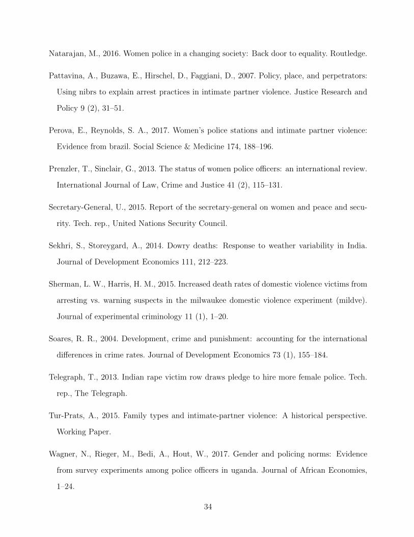
violence against women the fastest growing crime rate in the country– see Figure 1. One

explanation for this rise is attributed to an increase in women’s willingness to report crimes

as a result of improved political representation in local governments (Iyer et al., 2012). We

consider the role of the implementation of WPS as another explanation of this upward trend.

WPS is a form of policing that is widely used across the world and that typically involves

1A major example of this is the fact that the Security Council of the United Nations has taken severalinitiatives aimed at improving female presence in its missions and aimed at doubling the share of femalerepresentation by 2020 from of 10%.

2In India there is considerable awareness of this problem and one such example is the acknowledgmentcoming from the Prime Minister Narenda Modi where he stated on the International Women’s Day of 2015:”Our heads hang in shame when we hear of instances of crime against women. We must walk shoulder-to-shoulder to end all forms of discrimination or injustice against women” (The Hindu, 2015).

2

the creation of police stations that employ only female officers specialized in handling crimes

committed against women with a sensitive nature such as domestic violence, rape and other

forms of gender-specific offenses (Natarajan, 2016). The first WPS in the world opened in

Indian state of Kerala in 1973 and since then its use has been rolled-out to many other cities

in India (see Figure 3). As of 2013, India had 479 such stations spread out across most states.

This form of policing is expected to have a positive impact on service-provision to women

due to two main reasons. First, by lowering the costs of reporting a crime to the police

as WPS allow women to report a crime in an environment that is perceived as having less

stigma associated with gender-based crimes, less corrupt and more female-friendly (Miller

and Segal, 2014) 3. Second, there is abundant evidence from political economy that greater

in female representation improves the quantity and quality of the provision of public-goods

preferred by other women (Chattopadhyay and Duflo, 2004; Clots-Figueras, 2011; Matsa and

Miller, 2013; Bhalotra and Clots-Figueras, 2014; Ahern and Dittmar, 2012; Iyer et al., 2012).

We use a newly assembled data set on crimes at the city-level and, data at the state

and district-level we investigate how the placement of WPS changes crime rates of offenses

committed against women and arrests of these forms of crime. To identify the causal effect

of WPS, our identification strategy relies on exploiting the exogenous variation in various

forms of the introduction of the policy across cities, states and districts through differences-

in-differences models. First, we identify the effects of the placement of WPS across major

metropolitan cities in India and find that the opening of station increased reported crimes

committed against women in comparison to cities without a WPS. This increase is due to

changes in reports of domestic violence and female kidnappings.

Next, to supplement our city-level evidence, we exploit the variation in the implementa-

tion of the policy across states and years and find similar results as those of the effects at

3Anecdotal evidence that women prefer to discuss crimes committed against them of a sensitive naturewith other women are plenty (new, 2013, 2016; Telegraph, 2013). Qualitative evidence from the U.S. alsoreveals that officers stereotypes, education and race are major factors determining victim’s blame in rapeoffenses and the handling of cases (Pattavina et al., 2007; Burt, 1980).

3

the city-level. Finally, we look at the effects on arrest rates and find that in states where the

policy was first implemented arrest rates of female kidnappings also increased. This result

is consistent with the hypothesis that improvements in female police presence improve the

deterrence of gender-based crimes 4.

The main threat to our identification strategy is the presence of time-varying unobserv-

ables that correlated with both the placement of WPS and our main outcomes of interest,

i.e. measures of violence against women. To deal with this problem in our estimates include

state-linear trends in our estimations to account for any state-wide variation in unobservable

factors (e.g., implementation of other gender-based policies). Next, we test for the presence

of pre-trends and do not find evidence of its existence at the city or state-level. This is

consistent with qualitative evidence that shows that the decision to place WPS was part of

a complex process that is not correlated with previous crime rates or other gendered policies

(Natarajan, 2016).

Second, to understand whether our results are driven by changes in reporting behaviour

or incidence of violence against women (e.g., due to a backlash through improving women’s

representation) we investigate the effects of WPS on crimes whose reporting-bias is expected

to be lower (Iyer et al., 2012; Sekhri and Storeygard, 2014). We find that after the placement

of WPS female-specific mortality measures, including dowry death rates, did not vary. We

also find that individual level measures of self-reported incidence of intimate-partner violence

did not change. Next, using detailed police station-level data on reported crimes we find that

in urban areas (i.e., where WPS are available), reports of crimes committed against women

fell in general stations and this was accompanied by an increase in reports of this form of

4Following Becker (1968) a rise in the expected probability of punishment should decrease the supply ofcrime yet, empirical evidence for this result is mixed, and there is evidence of non-linear effects (Hjalmarsson,2008; Bindler and Hjalmarsson, 2017). The possible explanations that have been put forward for the lack ofresults or even counterintuitive results involve for example the increase learning of criminal behaviour dueto exposure to other criminals (Bayer et al., 2009). When it comes to domestic violence, there is limitedresearch on the deterrence hypothesis, and the evidence is mixed (Amin et al., 2016; Iyengar, 2009; Aizerand Dal Bo, 2009; Sherman and Harris, 2015). In this paper we interpret the rise in arrest rates as the initialeffects through which first there is an initial rise in arrest rates that as time passes leads potential offendersto change their decisions to commit a crime leading to fall in crime.

4

crime in urban areas where WPS are available. This effect is of 7 times larger in magnitude

which suggests that victims are more likely to report in WPS and that effects are not simply

due to a potential shift of cases across stations of different types. As a result, we attribute

our findings to a change in women’s willingness to report crimes rather than a change in

incidence of crimes committed against women which would require an effect on measures of

female mortality 5.

Finally, to ensure spurious results do not drive our findings (due to, for instance, changes

in policing practices) we investigate the effects of the placement of WPS on other non-gender

based crimes such as theft of riots and find that these were not affected by the placement of

WPS. To supplement our evidence at the city-level, we show two additional pieces of evidence

of the effects of WPS placement by looking at the effects at the state and district-level. The

main motivation for this is the fact that the policy was rolled-out outside of the sample

of cities we can test and for this reason, we also test if the policy also had similar effects

when we consider a wider policy variation definition. First, we use the variation at the state

and year level in the use of the policy over the period of 1988 and 2013. Consistent with

our previous results we find an increase in the rates of violence against women reports in

states that implemented the policy without any concomitant effects on other forms of crime.

Second, we use the fact that in the state of Jharkhand the use of WPS was rolled-out in

its districts in 2006 while in the neighbouring state of Bihar this policy was only in place in

2012. We use this feature and exploit the causal effect of WPS in districts in Jharkhand in

comparison to districts in Bihar 6 Our results are once again consistent with our previous

findings.

This paper adds to the growing literature on the economics of violence against women.

While recent evidence has focused on the role of income and unemployment in determining

5There is abundant evidence that lethal forms of crime are difficult to go undetected by the police andthus are less likely to be subject to measurement concerns such as changes in incentives to report.

6Jharkhand is a new state created by carving districts from the state Bihar in 2001. The use of this naturalexperiment has also been used to look at economic growth and political incumbency advantage (Asher andNovosad, 2015; Iyer and Reddy, 2013).

5

violence against women (Aizer, 2010; Anderberg et al., 2016; Bobonis et al., 2013), this paper

considers the role of bureaucratic representation in affecting women’s use of policing services a

feature that is of seldom consideration in the literature. The exceptions are (Kavanaugh et al.,

2017; Perova and Reynolds, 2017; Miller and Segal, 2014; Iyer et al., 2012)7. Kavanaugh et al.

(2017) use geo-coded information on the placement and timing of women’s justice centers

in Peru and find that after the opening of these centers domestic violence decreased. The

authors find that this is due to improvements in women’s female empowerment. Also, the

authors also investigate the effects on children’s educational outcomes and find large gains in

human capital accumulation. Our paper differs from that of Kavanaugh et al. (2017) is two

ways. First, WPS in India do not have a role beyond that of law and order, and for this reason,

its effects on other outcomes that go beyond reporting and police effectiveness are less likely

to exist. Next, our focus is on female empowerment through participation with the police

(as we look at measures of reporting and deterrence) a feature previously not considered yet

crucial in empowering women and deterring crime (Comino et al., 2016). Instead, Kavanaugh

et al. (2017) focus on measures of the self-reported incidence of intimate-partner violence.

Our paper is also related to Miller and Segal (2014) who investigate the effects of incorpo-

rating women in the police in the U.S. on reporting rates of domestic violence. The authors

use victimization and police-reported information to understand the effects of affirmative

action policies in between 1970 and 1990s that significantly raised the share of female officers

from 3.4 to 10%. The authors find that this increase led to a rise in reporting rates of domes-

tic violence incidents by 4.5 percentage points and a decrease in female homicides committed

by the intimate-partner. These results are consistent with a change in reporting behaviour

and an improvement in policing quality. This paper, like in ours and that of Kavanaugh

et al. (2017) and unlike that of Perova and Reynolds (2017), disentangles the reporting effect

from other unobservable changes that could have occurred (such as other improvements in

7Wagner et al. (2017) and Blair et al. (2016) use experimental data to look at the differential effects ofgender and ethnicity in policing. Wagner et al. (2017) find that female officers are no different than theirmale counterparts regarding malpractice. Blair et al. (2016) tests the effect of the ethnic composition ofpolicing teams in police effectiveness towards minorities.

6

policing) and also finds that the effects of improvements in female representation in the police

are concentrated in crimes committed against women.

This paper is also related to Iyer et al. (2012) who find that improvements in female

representation at the local level, increased reporting of crimes committed against women.

This effect is driven by improvements in female empowerment and exposure to women in

leadership positions. In our paper, we find that WPS improve the willingness to report a

crime but also its deterrence (through changes in arrest rates). Thus, our finding is likely

to be driven by changes in reporting behaviour but also in policing quality (as in Miller and

Segal (2014)).

This paper is related to two broad streams of literature. First, to the literature considering

the causes of crimes committed against women (Gulesci, 2017; Card and Dahl, 2011; Amaral

and Bhalotra, 2017; Tur-Prats, 2015; Iyer et al., 2012; Aizer, 2010; Borker, 2017) and in

particular we add to this stream of literature by looking into the role of deterrence policies

in effect this form of crime (Iyengar, 2009; Aizer and Dal Bo, 2009; Amaral et al., 2015).

Second, we add to the literature on female representation and targeting of public spending

and decisions that are more aligned with women’s preferences (Chattopadhyay and Duflo,

2004; Glynn and Sen, 2015) and general effectiveness due to better representation (Adams and

Ferreira, 2009). It contributes by looking at the role of gender-balanced police composition in

promoting safety for other women, a feature that has received little attention in development

despite crime reporting being considered a measure of trust and institutional development

(Soares, 2004; Banerjee et al., 2012).

This paper is organized as follows. In section 2 we provide a detailed description of female

representation in the police in India and the functioning of WPS. In section 3 we describe the

data and in section 4 the different identification strategies. In section 5 we present results

and section 6 concludes.

7

2 Background: Incorporation of Women in the Police

In India women, have been part of law enforcement since 1939 and this incorporation was

not initiated as a result of a specific policy. In fact, over the years, women were inducted to

the police due to the need to address the increase in female offenders and the rise in crime

committed against women (Natarajan, 2016). Despite the early introduction of women in

the police, the percentage of females in the Indian police force still averages less than 5%

between 2005 and 2013 (see Table 31). Within the country, the presence of women in policing

also varies substantially: from 8.4% in Tamil Nadu and 5% in Maharashtra to 1.6% in Uttar

Pradesh and 0.4% in Assam. Nonetheless, the share of female officers has risen sharply since

1990, a trend common to that in other countries (Miller and Segal, 2014) and that also follows

a general rise in police strength (Figure 2).

Regarding the distribution of female officers across ranks of the police, the share of women

is higher among the bottom and top rank positions.8 Over the period 2005-2013, the share

of women in these rankings has also increased but in a non-uniform way. For instance, the

share of Constables rose at a faster rate9. This is relevant given that it highlights the fact

that the introduction of female officers is not leading to a sorting into positions with lower

exposure to civilians. What’s more, this is consistent with the opening of WPS leading to

an increasing the need for female Constables.

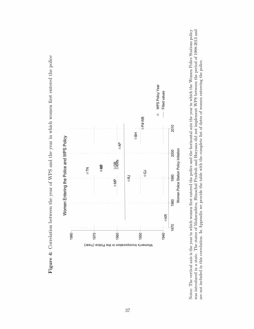
Finally, the timing at which women first entered the police force varies considerably across

states. In Kerala and Maharashtra women first entered the police in 1939. Delhi and Gujarat

followed in 1948 and, the last states incorporating women officers were Uttar Pradesh and

Tamil Nadu in 1967 and 1973, respectively. However, for most states, the implementation of

8Ranking of police positions in India is as follows: Director of Intelligence Bureau, Commissions of Policeor Director General of Police, Joint Commissioner of Police, Additional Commissioner of Police, DeputyCommissioner of Police, Superintendent of Police, Additional Superintendent, Inspectors, Sub-Inspectorsand Assistants to the Inspectors, Head Constables and Constables. Throughout the paper, we consider thesix highest ranks to be a single category, followed by a separate category of inspectors, a category of headconstables, and the remaining of constables.

9The information regarding police force by rank and gender is only available from 2005

8

WPS did not follow directly from this initial incorporation of women. For instance, Kerala

(the first state to open a WPS) did so 34 years since the initial incorporation of women in the

police. Tamil Nadu (the state with the highest numbers of WPS - about 40%), had a 19-year

gap between incorporating women and implementing WPS in 1992. This is important as

it suggests that (i) women were not incorporated in the police to serve only in WPS, and

(ii) the different forms of feminization of policing seem to be unrelated across states and

within states. We show in Figure 4 that indeed there is no correlation between women’s

incorporation in the police and the policy roll-out.

2.1 The functioning of women police stations

The use of specialized cells to deal with crimes of a sensitive nature such as committed against

women has been recommended since the National Police Commission of 1977 (Natarajan,

2016). These WPS are stations that typically (or tentatively) employ only female officers

and, only handle cases related to violence committed against women. For this reason, officers

placed at WPS receive specialized training in dealing with victims and in processing these

types of crimes. The purpose of these stations is to create a male-free environment where

women can report and be cooperative in the investigation. To our knowledge, these stations

do not have independent authority so that filing of cases and arrests should be approved by

the Head Constable of a general station.

The first WPS opened in Kerala in 1973. Since then, this form of policing spread across

the country and in 2013 almost all states had at least one WPS (see Figure 3). The growth in

WPS between 2005 and 2013 has been large and happened in all but two states: Maharashtra

and Himachal Pradesh (Table 26). Tamil Nadu is the state with the highest density of

stations, and these are well spread out across the state (Figure 3). These stations are generally

seen as a successful initiative by State Home Departments and for this reason there is a

staggering increase in WPS across the country (Department, 2012). This paper presents the

9

first comprehensive evaluation of the effects of WPS on crime and deterrence measures.

2.2 WPS and the reporting and recording of cases in India

In order to better understand the effects of WPS, we provide a brief description of the process

through which an offense would typically be dealt with. Once a crime occurs a victim can

decide whether to proceed to a station and report a case or not (reporting effect). Once in

a station, the attending officer must decide whether fill-in a First Investigative Report and

proceed with a formal investigation or not (recording effect). Finally, after an investigation,

officers may or may not make an arrest (effectiveness effect). The implementation of WPS

would make available to victim’s a more female-friendly environment that is specialized in

dealing with cases of violence against women. Thus, we expect that following the roll-out of

a WPS reports of VAW crimes increase. Second, because in WPS officers are less likely to

exhibit skewed gender norms about the roles of women or tolerance of violence committed

against them, we expect that the recording and subsequent filling of FIR’s to increase. Finally,

if female officers increase the effort in investigating these types of crimes and/or the actual

form of policing makes crime investigation more simple than we would expect a rise in the

effectiveness in handling of these crimes.

In our data we only fully observe some of the stages. First, in the first phase, crime report-

ing is a latent variable that one could only measure through victimization data. Nonetheless,

since we do observe crimes with different levels of reporting incentives (e.g. domestic violence

versus female mortality) we attempt to address the first effect by looking at different forms

of crime. Next, we use information at the state-level on charge-sheet rates and arrest rates

to investigate the effects on the two remaining variables. This process follows closely Iyer

et al. (2012) where we use the author’s data and extend it to 2013.

10

3 Data

Women police stations. The information on the dates of opening of WPS in cities and

of the roll-out of the policy was gathered from multiple sources. The main source is the

yearly reports on Policing Organization from the Bureau of Police Research and Development

(BPRD). These reports contain the city location of stations across India and its year of roll-

out since 2005. We use this information to provide a detailed description of the path of WPS

implementation over the period of 2005 and 2013. We combine this information with crime

records data from the major metropolitan areas in India. This information was collected from

the National Crime Records Bureau (NCRB). It is worth noticing that, while there are many

more cities with WPS we are restricted to the cities contained in the NCRB publications .10

This data is used in the city-level analysis.

For the state-level analysis, we gathered information about the timing of adoption of WPS

across states from the BPRD reports and (Natarajan, 2016). Since most states, implemented

WPS before 2005 we complement the remaining data by contacting each state Ministry

of Home Affairs and Police Headquarters separately 11. The variation in WPS policy are

presented in Table 25.

Crime. We make use the National Crime Records Bureau (NCRB) yearly data. The NCRB

provides data from police-reported crimes for cognizable crimes prescribed under the Indian

Penal Code. This is the major source of administrative data on law and order in India. The

data is based on information gathered from two processes. First, once an incident occurs

and is reported, the police are required to register a First Information Report (FIR) - see

Iyer et al. (2012) for an overview. Second, this information is aggregated by each police

10Information at the city-level from India is known for being difficult to gather (Greenstone and Hanna,2014) and we are not aware of any other publicly available source of information on crimes we could use. Tothe best of our knowledge, this is the one of the most comprehensive city-level panel data sets assimilatedand analysed for India to date.

11We also cross-checked our information with media dissemination information on the opening of WPS’s(or Mahila Thana’s in Hindi)

11

station and then reported to the NCRB that then aggregates it at different levels. We use

this information from 2005 to 2013 for the city-level analysis and from 1988 to 2013 for the

state-level analysis.

The NCRB provides data for 18 categories of crime which we use to construct three

major crime categories. These are violence against women, non-gender based violence, and

property.12 The release of each crime category varies over time with rape being consistently

reported over the years, female kidnappings started being reported as a separate category

since 1988, and the remaining categories in 1995. These differences do not affect our estima-

tions since we always include year dummies, but they condition the categories we are able

to track over time since 1988. Figure 1 shows the trend in the three major crime categories

since 1995. Over the period, reports of violence against women have risen and at a faster

rate than the remaining categories.

The crime data in city-level analysis makes use of the statistics from the metropolitan

areas database. Also, to increase the sample of cities, we also combine this information with

the statistics available from the crime area-level database. Overall, our sample consists of

an unbalanced sample of 76-89 cities. The list of cities by year is provided in Table 30 is

in Appendix. The data from our state-level analysis is from the state-level statistics and is

available since 1988 i.e. the year at which we have at least two categories of crime we can

track.

In cities, over the period, the rate of crimes committed against women per 100,000 popu-

lation was of 534. This rate is considerably higher in cities with a WPS (626) when compared

to those that do not have a WPS (188). Within the category of violence against women, the

rate of domestic violence is the highest with 330 reports per 100,000 population. In spite of

its fastest growth, the rate of property and non-gender based violence is higher. On average,

12VAW includes domestic violence, rape, molestation, sexual harassment, kidnapping of women and girls.Non-gender based violence includes murder, riots, kidnapping of males, dacoity, arson and hurt. Propertycrime includes theft, robbery and burglary. A detailed description of these categories can be found in theIndian Penal Code.

12

there are 2187 reports of property crimes per 100,000 population and 2137 of non-gender

based violence. These rates are also higher across cities with and without a WPS (Table 31).

To explore mechanisms, we also collect crime-specific arrests and charge-sheeting rates

from the NCRB reports. This data is only available at the state-level. Moreover, we also col-

lect information on gender-specific mortality available at the state-level cause (i.e. accidental

deaths, dowry deaths, suicides or murder due to love affairs).

Demographic, political and law and order data. We gather relevant demographics

including total population, gender and caste composition and literacy to be used as control

variables. These data is collected from the urban agglomeration and state-level Census data

of 1991, 2001 and 2011. We interpolated the data for the remaining intervening years. We

also gather information on police strength by gender and rank from the annual reports of

the NCRB and BPRD. We also include a dummy for state election years gathered from the

Election Commission.

4 Identification Strategy

To investigate the effects of increased presence of women in the police through the imple-

mentation of WPS, we make use of a difference-in-differences identification strategy applied

to the distinct levels of aggregation of the data (as explained before these are city and state.

This is done for two main reasons. First, because while WPS are mostly implemented in

cities in many states the policy was expanded to other urban and rural areas that we cannot

identify in the sample of the crime data at the city-level. Thus, to be precise about the

effects of the policy we extend our main analysis to a state-level analysis. The second reason

is data driven. While the WPS policy started in 1973, we are only able to match crime and

city-level since 2005. To take advantage of the information we gathered on the year in which

states started implementing WPS we also show results that make use of information since

13

1988 up to 2013.

First, we will exploit the staggered implementation of WPS in Indian cities. Second, by

investigating the roll-out of the policy across districts and states. We describe each of the

identification issues and empirical strategy below.

City-Level Analysis

Using city-year data and the precise information on the year of the introduction of women-

only stations, we estimate the change in reported crime rates across before and after the

placement of WPS in comparison to cities that did not open WPS. The estimating equation

is as follows:

Crimecst = α0 + δ1PostWPSct + βXct + βXst + γc + λt + φct+ εcst (1)

where Crimecst is the crime rate per 100,000 population (in logarithms) in city c of state

s measured in year t. The variable PostWPScst is a dummy that takes the value one in

the years following the opening of a WPS in given city c. In our specification, we include

a vector of city-level controls (Xcst) that include the ratio of males to females to take into

account for the demographic gender inequalities that have been shown to have a positive

effect on gender-specific crimes (Amaral and Bhalotra, 2017). We also include literacy rate

to take into account for the underlying differences in the willingness to commit crime and

reporting behaviour (Erten and Keskin, 2016). Finally, at the city-level, we also take into

account for the differences in management of policing by including a dummy as to whether

the city has a Police Commissioner system. We also take into account for differences in

cities across states by including as controls factors that could impact upon crime differently

(e.g. the share of female officers). In addition to this, we also include a rich set of fixed-

effects. We include city fixed effects, γc to control for permanent unobserved determinants of

gender-based violence across cities (Tur-Prats, 2015; Alesina et al., 2016); year fixed effects to

14

non-parametrically adjust for national trends in crime and, city-linear trends (φct) to adjust

omitted time-varying factors in cities across. The coefficient of interest is δ1 measures the

differential effect of implementing a WPS within c in a year t in comparison to other cities in

that same year. All standard errors are clustered at the city-level and regressions to account

for possible correlated shocks to city-level crimes over time. All regressions are weighted by

population size. The term εcst is the idiosyncratic error term.

State-Level Analysis We use the timing and state variation in the initiation of the roll-out

of WPS in states as a natural experiment to identify the effects on gender-specific crime. We

follow a difference-in-differences strategy similar to (1) but where we exploit the variation in

the policy roll-out:

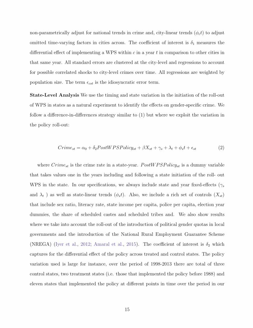
Crimest = α0 + δ2PostWPSPolicyst + βXst + γs + λt + φst+ εst (2)

where Crimest is the crime rate in a state-year. PostWPSPolicyst is a dummy variable

that takes values one in the years including and following a state initiation of the roll- out

WPS in the state. In our specifications, we always include state and year fixed-effects (γs

and λt ) as well as state-linear trends (φst). Also, we include a rich set of controls (Xst)

that include sex ratio, literacy rate, state income per capita, police per capita, election year

dummies, the share of scheduled castes and scheduled tribes and. We also show results

where we take into account the roll-out of the introduction of political gender quotas in local

governments and the introduction of the National Rural Employment Guarantee Scheme

(NREGA) (Iyer et al., 2012; Amaral et al., 2015). The coefficient of interest is δ2 which

captures for the differential effect of the policy across treated and control states. The policy

variation used is large for instance, over the period of 1998-2013 there are total of three

control states, two treatment states (i.e. those that implemented the policy before 1988) and

eleven states that implemented the policy at different points in time over the period in our

15

sample13. Standard-errors are clustered at the state-level.

In both (1) and (2) we are able to address the plausible sources of endogeneity through

the introduction of a rich set of controls, fixed-effects and area-specific linear trends. As a

result, we take our model to accurately capture the causal effect of the implementation and

roll-out of WPS. To further inspect that our results are not biased due to omitted trends

we first provide test for the presence of pre-existing trends. Next, we inspect whether the

implementation of WPS have an effect on crimes that are not expected to change with this

policing form. The failure to reject that WPS lead to changes in non-gender specific crimes

would be suggestive of the presence of omitted factors that are common to all forms of

crime. Finally, the remaining possibility is the presence of omitted trends that are specific to

gendered crimes. To inspect for this we look at the effects on other forms of crime that are

gender-specific but are not expected to vary with a change in the incentives to report crimes.

5 Results

Determinants of Placement of Women Stations and Parallel Trends.

Since our main identification strategy relies on a difference-in-differences experiment, we

start by presenting some evidence on its exogeneity. First, we start by showing that there

is no apparent correlation between the year’s states incorporated women in the police and

the use of the WPS policy – see Figure ??. Next, we estimate the determinants of the

placement of stations in cities and, of the determinants of the roll-out of the policy in states,

respectively show in Tables 1 and 2. In both, we regress the potential determinants of a

dummy variable that takes values one if in a given city-year or state-year there is a WPS.

13The states included in the sample are Andhra Pradesh, Bihar, Gujarat, Haryana, Himachal Pradesh,Punjab, Madhya Pradesh, Rajasthan, Uttar Pradesh, Karnataka, Kerala, Tamil Nadu, West Bengal. Thenewly created states of Telangana, Jharkhand, Chhattisgarh and Uttaranchal are merged with their pre-2001state boundary definitions. Since Jharkhand initiated the policy prior to the state of Bihar in this case wetake the year of 2006 as the year in which the policy had an effect for the state of Bihar under the pre-2001boundaries definition.

16

In Table 1, in column (1) we only include a set of socio-demographic factors, and we do not

find that there is a correlation between these factors that include sex ratio and literacy rate,

and the placement of cities. Next, we include, separately, the share of female officers in the

state, whether the city has a Police Commissioner system and, the lag of the crime rate of

violence committed against women. These results are reassuring that the placement is not

correlated with factors and instead is the results of a complex decision process.

When considering the determinants of the policy across states (in Table 2) we find con-

sistent results when considering socio-demographic correlates. However, we find that the

probability of states implementing WPS is decreasing with income per capita; increasing

among the states that are most effective in implementing the NREGA and, decreasing in the

in states where the local gender political quotas where first implemented. Together these do

not show a clear understanding of the underlining causes of states implementing WPS. On

the one hand, richer states are less likely to use this form of policing, but at the same time,

the implementation of NREGA could have raised the need to improve the response to in-

creasing in crimes committed against women because of the programme as shown in Amaral

et al. (2015). On the other hand, it could be that there is some level of competition between

gendered policies so that in states where female representation in politics has implemented

the roll-out of WPS was neglected. To take these factors into account, we include these

controls separately in the regressions.

For our estimates in (1) and (2) to be valid the required identifying assumption is that

treated units (those implementing WPS) and control units must have parallel trends in the

main outcome of interest – total rate of crimes committed against women. Our estimates

of δ1 and δ2 will be biased if control units do not resemble treated units. In Figures 5 and

6 we provide event-study estimates of the effects of WPS in the city and state samples,

respectively. It is apparent from these that areas implementing WPS were no different in the

pre-period as the coefficients for years before the policy are insignificant. Also, we can see

that there is a clear positive effect of the policy that is immediate and remains positive in

17

the years following the placement of WPS.

To the best of our knowledge – from discussions with officers- the decision to implement

a WPS is part of a complex decision process that involves locations expressing an interest in

this form of policing with interest in the same direction from high-ranking police officials and

state ministers. Thus, our results are consistent with the fact that plausible determinants of

WPS placement do not seem to predict its placement at a given time. Taken this, we now

turn to our difference-in-difference estimations results.

5.1 Effects on crime

City-Level Analysis. We present the results from estimating (1) in Table 3. In Panel A

we present results where the primary dependent variable is the total rate of reported crimes

committed against women and in Panel B total rate of non-gender based violence. Moving

from columns 1 to 6 we enrich the specification by first including a set of baseline controls

in addition to city and year fixed-effects; next, by including state-linear trends in column

3; controlling for Police Commissioner system in column 4; controlling for the state share

of female officers in column 5 and, finally in column 6, our preferred specification where we

include city-linear trends.

Across specifications, we find a positive statistically significant effect on total crimes com-

mitted against women with coefficient ranging from 0.5 in the specification without controls

to 0.2 in the most parsimonious estimation. Regarding effect sizes, in treated cities, the

increase in the rates of violence committed against women was of 21.4%. In column 5, it is

reassuring to see that the inclusion of the total share of female officers does not affect the

direction and magnitude of the results. The result suggests that the effect of WPS is in the

form of policing rather than the share of female officers.

Looking at the effects of opening a WPS on non-gender based violent crimes (Panel

18

B) the effects are not statistically significantly different from zero and importantly, these

coefficients are nearer to 0 as we improve the specification (column 3-5). These results

suggest that opening WPS led to an increase in gender-specific crimes and was not due to

other unobservable changes that could affect all forms of crime. Also, since these effects are

concentrated on gender-specific crimes, this placebo results confirm our hypothesis that WPS

led to a change in women’s willingness to report and not necessarily the existence of male

backlash that could have also led to a rise in general crimes. We also test for the effect of

WPS in additional crime types (of violence and property crime types) Table 28 in Appendix.

Across all 8 different crime rates, we do not find that opening of a WPS change these crimes.

This is consistent with previous results in Table 3 and also reassures that WPS did not

change other crime types that should not be affected by an increase in incentives for women

to report crimes committed against them. This ensures that our results are not driven by

a spurious correlation or omitted factors that could affect all crime types equally within the

same city-year.

Next, we look at the effects by crime type by disaggregating the rate of total violence

against women into its singular component categories to understand which type of crime was

more affected. We present these results in Table 5. The variables of interest are the rates

of female kidnappings, domestic violence, dowry deaths, molestation, sexual harassment and

rape. We find that the effects of WPS are due to increases in the rates of female kidnappings

and domestic violence with increases of the magnitude of 22.2% and 21.7%, respectively. This

finding seems to suggest that reporting incentives are likely to matter more among crimes

with a medium range of severity and not all forms of crime against women.

Finally, we repeat the test of pre-trend presented in Figures 5 in Table 5. For our main

variable of interest, total rate of violence committed against women, we do find evidence of

pre-trends in the year preceeding the policy or two years before.

State-Level Analysis. We present the results for the state-level analysis – specification (2)

19

in Table 6. In Panel A the main dependent variable in the total rate of violence committed

against women; in Panel B the rate of female kidnappings and Panel C Rape rate14. Moving

from column 1 to 2 we include the set of socio-economic controls in addition to state and year

fixed-effects. In column 3 we also include police force per capita and a dummy for election

years in the states. In column 4, we add state-linear trends. In column 5, we control for the

local gender political quotas reform following Iyer et al. (2012). In column 6 we control for

the differential effect of the NREGA reform and column 7 we also control for the share of

female officers in the police in each state-year.

We find that states that started implementing WPS, the total rate of crimes committed

against women increased by 22.5%. This increase in partially due to a rise in the rate of

female kidnappings which increased by 10.85%. As per before, we do not find a statistically

meaningful change in the rate of rapes. As suggested before the reform could have had a

larger impact in crimes with lower cost of reporting in comparison to others whose emotional

and physical costs is potentially higher as is the case of rapes.

As per before, we reiterate this analysis on crimes which are not likely to change as a

result of WPS. We present these in Table 21 in Appendix. We consider as dependent variables

the rate of male kidnappings, dacoity, robbery, burglary, thefts and total male deaths. We

do not find evidence that in states implementing WPS non-gender specific crimes changes.

This placebo test ensures the validity of our estimations.

As a robustness exercise, in columns 8-10 we repeat the main regressions by excluding the

state of Tamil Nadu. This state is unlike any other state in the sense that it implemented the

WPS policy in an unprecedented form 3. This state has 41% of all WPS in the country and

these are evenly distributed within the state. To understand whether our results are driven

by the intensity of the treatment in Tamil Nadu we estimate (2) without it. Our results are

not sensitive to the exclusion of this state which shows the importance of the effectiveness of

14Due to differences in the way crime data was released over time in India we can only track these 2 singlecategories over the period of 1988-2013

20

WPS beyond the intensity of the placement.

Finally, we also present a test of the effect of the reform in the years preceding the roll-out

of the policy – see Table 7. As suggested in Figures 6 we do not find evidence of differential

pre-trends in year before the initiation of the policy, 2 years or 3 years. In Appendix we also

present the estimation of (2) with all coefficients. Results are consistent with those find by

others - see Table ??.

Additional Evidence: The cases of Jharkhand-Bihar. To make use of the full extent

of the crime data and to further supplement the validity of our results we exploit the effects

of the roll-out of WPS using an additional natural experiment. In 2001, three states were

created from districts of three largest states. The state of Jharkhand was one of these newly

created states that was split from districts of the state of Bihar. This experiment is of

interest to this paper as Jharkhand, unlike its former state of Bihar, opened WPS in each

of its districts in the year 2006. Thus, we make use of the fact that districts in Jharkhand

are likely to be similar in terms of unobservable factors since these were previously under

the same state and exploit this feature by comparing the change in crime rates in districts

of Jharkhand in comparison to districts in the state of Bihar. The identifying assumption

is that districts in Jharkhand would have had the same trend in crime as its counterpart

districts in the state of Bihar had it not been for the placement of WPS in the newly created

state.

We make use of the district-level data from the NCRB from the years 2001-2011. This

implies that in our sample there are 5 pre-treatment years and 6 post-treatment periods and

22 districts in Jharkhand in comparison to 37 in Bihar. In our analysis, we also include

similar control variable as those in (2). These are collected from district-level Census for the

years 2001 and 2011. In Table 24 we present summary statistics. In Figures ?? we present

the means in the total rate of crimes committed against women in the pre and post period.

The rightest panel shows the difference in means. As it is clear there is a rise in these rates

21

in districts in Jharkhand. In Table 12 we present differences-in-difference estimation results

of the following equation:

Crimedst = α0 + δ3Jharkhandds × Postt + α1Postdt + βXdt + γd + λt + φst+ εdst (3)

where Crimedst is the crime rate in a district, state, year. The variable Jharkhandds takes

values one if a district is in the state of Jharkhand and Postt is a dummy variable that takes

value one after the year 2006. Thus, δ3 is the difference-in-difference coefficient capturing

the differential effect of the WPS across treated (districts in Jharkhand) and control states

(districts in Bihar) before-after the placement of WPS15. The coefficient α1 captures for the

post-2006 general effect on crime in the control districts i.e. those in the state of Bihar that

did not receive a WPS. The vector Xdt is a vector of socio-economic controls that include sex

ratios, literacy rates and share of scheduled castes and tribes. We also include district fixed-

effects (γd) and year dummies (λt). We also include a set of state linear trends to account

for differences specific to each state over time (φst). All standard-errors are clustered at the

district-level. The term εdst is the error term.

Table 12 presents the results for rate of total crimes committed against women and the

individual categories of rape, female kidnappings, domestic violence, sexual harassment, mo-

lestation and dowry deaths. Panel A considers only the sample of neighbouring districts, i.e.

those that would be most similar regarding time-varying unobservables. Panel B considers

the full sample of districts in each state. We find that the placement of WPS led to an in-

crease in reports of total crimes committed against women, female kidnappings and domestic

violence. The coefficients in Panel A are marginally insignificant but we consider this is due

to the small sample size (N=198) as the coefficients in Panel A is similar in magnitude but

15We provide results using the sample of bordering districts to Jharkhand and Bihar and also separately,for all district in both states. In this case, the variable Jharkhandds takes values one if a district is in thestate of Jharkhand and borders Bihar or zero if it is a district in Bihar that broders Jharkhand.

22

statistically significant. We find a positive and statistically significant effect on the rate of

total violence against women, female kidnappings and domestic violence. The failure to in-

clude state linear trends (columns 2) affects our estimates in the sense that its omission leads

to an underestimate of the effects of WPS. Regarding effect sizes, the placement of WPS led

to an increase in the rate of total crimes committed against women by 30% - a magnitude

consistent with our findings in the city sample. Moreover, WPS led to an increase in the rate

of reports of female kidnappings by 41% and of domestic violence by 87%.

6 Channels of Transmission

6.1 Do WPS lead to a change in the incidence or reporting be-

haviour of VAW?

Effects on female mortality rate. In Table 8 we look at the effects on female mortality

outcomes. We construct a measure of female mortality that is the sum of police cases by state-

year of murders due to love affairs; female suicides; and accidental deaths. Since homicides

committed by the intimate-partner is the leading cause of female homicides and given the

fact that there is a low probability that deaths go unaccounted for, we use this measure to

capture for the incidence of VAW rather than changes in reporting behaviour of women. We

find that WPS did not change female mortality. This is consistent with WPS having affected

crimes that are more likely to change with reporting incentives rather than instigating a

change in incidence of VAW that would also affect female mortality rates.

Effects on measures of self-reported intimate-partner violence. We also exploit the

variation in state-level exposure to the policy across residents in urban and rural areas using

individual-level data from the Demographic and Health Surveys of 2005-2006 and 2015-16.

The use of this information is informative due to two main aspects. First, we can consider a

23

measure of self-reported intimate-partner violence, a measure that is typically considered to

be subject to less measurement error 16. Second, within the space of the ten years of the survey

rounds, five states have adopted the WPS policy; and the remaining three states have not

implemented the policy. This coupled with the fact that the WPS policy is present in urban

areas and not rural areas allow us to identify the effect of the policy using a triple difference-

in-difference estimation strategy whereby we use as identifying factors (i) treatment and

control states; (i) the timing of the policy roll-out and, (iii) whether the respondent resides

in urban or rural areas. We present this variation in Table 33. Using this we then proceed

to estimate the following triple difference-in-difference model:

IPVisy = α0+δ1Treatments×Posty×Urbani+β1Treatments+β2Posty+βXi+γs+λy+εisy

(4)

where IPVisy the is the self-reported measure of intimate-partner violence (IPV). The coeffi-

cient of interest is δ1 that captures for the differential effect of the roll-out of the WPS policy

in treatment states Treatments, before-after its implementation Posty which we measured

using the year of implementation of the survey and the roll-out of the survey. Finally, since

the policy was only implemented in urban areas, we also exploit the additional source of

variation coming from residents in urban versus rural (Urbani). To account for unobserved

confounders, we also include a vector of woman-specific characteristics that include age, caste

and religion dummies, household size, and separately female years of education, number of

children born. We present these findings in Table 32. Across specifications, we do not find

evidence that women’s exposure to domestic violence changed and this result does not dif-

fer across forms of IPV (emotional, physical or sexual) or the inclusion of state-urban area

dummies that would account for additional unobserved factors that could affect women in

urban versus rural areas within the same state.

16This measure is more likely to be a better candidate to measuring incidence of intimate-partner violence(i.e. domestic violence) because it has less reporting costs (e.g. going to a police station). Yet, socialdesirability bias and stigma are also factors that may affect the measurement of this variable and for thisreason we also present results using female mortality measures.

24

Put together these results suggest that the implementation of WPS led to a change in

measures of VAW that are sensitive to reporting incentives rather than a change in incidence

of violence that would likely affect female mortality rates or self-reported intimate-partner

violence.

6.2 Testing the effect on women’s willingness to report in WPS.

Evidence from police station-level data. To further show that the results found for

measures of VAW that are sensitive to changes in reporting incentives rather than incidence

we exploit how reports of VAW to the police changed across stations, i.e. women-only police

stations and general stations. We use the data collected by (Banerjee et al., 2012). This

data contains information on 73,207 police reports collected from 152 police stations, across

ten districts of Rajasthan in the years of 2006 and 2007. We coded VAW crimes following

the definitions of the Indian Penal Code. 17. We then estimate a cross-sectional difference-

in-difference model whereby we compare how reports of VAW within treatment districts in

Rajasthan (i.e. 4 treatment districts) vary in comparison to reports in stations in control

districts (i.e. 6 control districts). We estimate the following:

Crimesdt = α0+δ1Treatmentd×Urbans×WPSs+δ2Treatmentd×Urbans+γd+λt+εsdt (5)

where Crimesdt is the total number of reports to station s in district d during month t. The

coefficient of interest is δ1 that captures for the differential effect in police reports of VAW

across districts implementing the WPS policy (Treatmentd), in urban and rural stations

(Urbans) and across WPS and non-WPS stations. The coefficient δ2 represents the effect

on general stations. We always include district and month-year fixed effects and weight the

17Defined as crimes coded as cases that fell under the category of cruelty towards wife (domestic violence);rape; molestation; the Dowry and Woman Act; and cases coded as 493, 494, 495, 496, 497, 498, 509 alldefined as crimes committed against women under the Indian Penal Code. This totalized 6,124 reports(approximately 9.3% of all crimes which is comparable to NCRB statistics.

25

regressions by district population as measured in the Census 2011. In separate estimations,

we also include a monthly station trend and separately district*month-year fixed effects that

would absorb any district unobserved effects at the month-level. Standard-errors are clustered

at the station-level.

Due to the richness of the data we are also able to test for the effects of WPS on two

separate aspects. First, we validate if changes in women’s willingness to report in WPS

raises the total reports of VAW crimes (as we have otherwise shown before). This is identify

through coefficient δ1. Second, we test if women move away from reporting in general stations

to reporting in WPS. This would imply that δ1 is positive (i.e. the increase in reports effect)

and that δ2 is negative. Importantly, if the magnitude of δ1 is larger than δ2 this would mean

that not only WPS lead to a direct shift of cases from general to WPS’s but indeed evidence

of additional reports being reported in WPS that would have not been reported in general

stations in the absence of the policy.

We present these results in Table 9. Consistent with our hypothesis we find a significant

and positive coefficient for δ1 and negative coefficient for δ2 for the crime categories of total

VAW and domestic violence. It is also worth noticing that coefficients are largely unchanged

with the inclusion of state trends (columns 2) and district-year dummies (3). The magnitude

of the coefficient is of about 8.35 additional reports in WPS’s, and a decrease of 1.35 reports

in general stations. This represents an additional 7 reports in WPS.

Finally, we also implement an additional test where we look only at the effect in general

stations, across treatment and controls districts across urban areas viz.a.vis the rural station’s

counterparts. These results are shown in Table ??. We show that the coefficient of the effect

of general stations in urban areas is very similar to coefficient δ2 shown in Table 9. Second,

the coefficients for rural areas are not statistically different between treatment and control

districts. This falsification exercise allows showing evidence that there are no potential

unobserved confounders between districts implementing WPS and those that did not.

26

Evidence from self-report measures of use of support services. A theory of change

of VAW involves the development of pro-active behaviours that eventually lead to a decrease

in VAW. A change in women’s willingness to report VAW crimes as a result of the WPS

would, therefore, be consistent with women being more likely to seek for support in their

social networks (i.e. friends) or along formal services. To test for this, we follow the same

identification as in model (4) and use as dependent variable a measure of self-report use

of formal or informal support services. This module is asked to a small sample of women

who respond to have been victims of intimate-partner violence and asks respondents about

whether they have mentioned the problem to family members (including the partner and

former partner); police; a neighbour; social organisation; lawyer; religious leader or a doctor.

We run regressions of the form of (4) and test if women affected by the WPS were more

likely to use support services. We construct an index of usage of support services that range

from 0 (no use) to 7 (use of all modes of support services) and also a dummy variable if

the respondent used at least one form of service. We present these results in Table 10. We

find that usage of support services increased which is consistent with the WPS leading to

an overall change in pro-active behaviours that is correlated with increases in reports to the

police.

6.3 Effects on deterrence measures.

In Table 11 we consider the effects of WPS on police effectiveness. We hypothesise that

WPS rise the overall quality of police in handling gender-based crimes as the creation of

WPS facilitated a more female-friendly space for victims to cooperate with the police and

also, the availability of police staff specifically trained to handle these types of offences. We

find that after the implementation of WPS in states 18 arrest rates due to female kidnappings

increased by 15%. This is consistent with our finding from Table 6 that after a rise in reports

of female kidnappings, policing treatment of these type of offence also increased. This result is

18Information on arrests and charge-sheet is only available at the state-level.

27

important given the fact that improving women’s access to justice is not a sufficient condition

to deter crimes committed against women. Deterrence of this type of offence, much like other

crimes, is required for total incidence to decrease.

As a robustness exercise, we exclude the state of Tamil Nadu. This state is unlike any

other state in the sense that it implemented the WPS policy in an unprecedented form 3.

This state controls 41% of all WPS in the country, and these are evenly distributed within

the state. In order to understand whether our results are driven by the intensity of the

treatment in Tamil Nadu we estimate (2) without this state. Our results are not sensitive to

the exclusion of this state which shows the importance of the effectiveness of WPS beyond

the intensity of the placement.

These results are also consistent with evidence from the U.S. showing that increases in

the presence of female officers led to increases in the rate of reporting of cases of domestic

violence which led to a subsequent decline in incidence Miller and Segal (2014). In addition,

these finding are also in line with those of Amin et al. (2016) who show, using cross-country

data that, improvements in protective domestic violence legislation would have saved about

33 million women between 1990 and 2012.

7 Conclusion

Violence against women and girls (VAWG) poses a major obstacle to achieving inclusive

prosperity and ending poverty. This type of violence is arguably hindering social and eco-

nomic development and its repercussions for long-term development are large. Across the

globe, estimates show that nearly 1 billion women will experience intimate partner violence

or non-partner sexual violence in their lifetime. Moreover, homicides committed by partners

remain one of the highest causes of female mortality Garcia-Moreno et al. (2006); Amin et al.

(2016) .

28

This paper investigates how improvements in female representation in policing impacts

upon the rates of crimes committed against women and its subsequent arrests. Our findings

show that the implementation of women police stations in India led to significant increases

in the rate of crimes reported to the police in the order of magnitude of 22% rise. This in

turn led to a rise in arrests of crimes whose reports increased.

The policy we investigate is one of low intensity and in a context of women-only police

stations with limited resources. Yet, in spite of this we find results that improvements in

access to justice can rise women’s willingnes to approach law and order services. This feature

is core in economic development models but there was limited evidence for this when it comes

to addressing violence against women Soares (2004). This paper addresses this issue for a

sample cities and states in India.

Our paper makes a contribution to the literature on crime and violence against women by

showing how improvements in women’s access to justice and quality of police service provision

can impact upon deterrence of crimes committed against women-one of the most under-

reported forms of crime. Across the globe women are under-represented in law enforcement,

this shows that the inclusion of women in this traditionally male occupation can improve

women’s access to justice and help deter future crime.

29

References

, 2013. More female police officers are needed to end violence against women in afghanistan.

, 2016. Why aren’t u.s. police departments recruiting more women?

Adams, R. B., Ferreira, D., 2009. Women in the boardroom and their impact on governance

and performance. Journal of financial economics 94 (2), 291–309.

Ahern, K. R., Dittmar, A. K., 2012. The changing of the boards: The impact on firm

valuation of mandated female board representation. The Quarterly Journal of Economics

127 (1), 137–197.

Aizer, A., 2010. The gender wage gap and domestic violence. The American Economic Review

100 (4), 1847.

Aizer, A., Dal Bo, P., 2009. Love, hate and murder: Commitment devices in violent relation-

ships. Journal of public Economics 93 (3), 412–428.

Alesina, A., Brioschi, B., Ferrara, E. L., 2016. Violence against women: A cross-cultural

analysis for africa. NBER Working Paper w21901.

Amaral, S., 2017. Do improved property rights decrease violence against women in india?

ISER Working Paper Series- forthcoming.

Amaral, S., Bandyopadhyay, S., Sensarma, R., 2015. Employment programmes for the poor

and female empowerment: the effect of nregs on gender-based violence in india. Journal of

interdisciplinary economics 27 (2), 199–218.

Amaral, S., Bhalotra, S., 2017. Sex ratio and violence committed against women: the long-

run effects of sex-selection in india. mimeo.

Amin, M., Islam, A. M., Lopez-Claros, A., 2016. Absent laws and missing women: can

domestic violence legislation reduce female mortality?

30

Anderberg, D., Rainer, H., Wadsworth, J., Wilson, T., 2016. Unemployment and domestic

violence: Theory and evidence. The Economic Journal 126 (597), 1947–1979.

Asher, S., Novosad, P., 2015. The impacts of local control over political institutions: Evidence

from state splitting in india. Unpublished manuscript.

Banerjee, A., Chattopadhyay, R., Duflo, E., Keniston, D., Singh, N., 2012. Improving police

performance in rajasthan, india: Experimental evidence on incentives, managerial auton-

omy and training. Tech. rep., National Bureau of Economic Research.

Bayer, P., Hjalmarsson, R., Pozen, D., 2009. Building criminal capital behind bars: Peer

effects in juvenile corrections. The Quarterly Journal of Economics 124 (1), 105–147.

Beaman, L., Chattopadhyay, R., Duflo, E., Pande, R., Topalova, P., 2009. Powerful women:

does exposure reduce bias? The Quarterly Journal of Economics 124 (4), 1497–1540.

Becker, G. S., 1968. Crime and punishment: An economic approach. In: The economic

dimensions of crime. Springer, pp. 13–68.

Bhalotra, S., Clots-Figueras, I., 2014. Health and the political agency of women. American

Economic Journal: Economic Policy 6 (2), 164–197.

Bindler, A., Hjalmarsson, R., 2017. Prisons, recidivism and the age–crime profile. Economics

Letters 152, 46–49.

Blair, R. A., Karim, S., Gilligan, M. J., Beardsley, K. C., 2016. Policing ethnicity: Lab-

in-the-field evidence on discrimination, cooperation and ethnic balancing in the liberian

national police.

Bobonis, G. J., Gonzalez-Brenes, M., Castro, R., 2013. Public transfers and domestic vio-

lence: The roles of private information and spousal control. American Economic Journal:

Economic Policy, 179–205.

31

Borker, G., 2017. Safety first: Perceived risk of street harassment and educational choices of

women.

Brollo, F., Troiano, U., 2016. What happens when a woman wins an election? evidence from

close races in brazil. Journal of Development Economics 122, 28–45.

Burt, M. R., 1980. Cultural myths and supports for rape. Journal of personality and social

psychology 38 (2), 217.

Card, D., Dahl, G. B., 2011. Family violence and football: The effect of unexpected emotional

cues on violent behavior. The Quarterly Journal of Economics 126 (1), 103–143.

Chattopadhyay, R., Duflo, E., 2004. Women as policy makers: Evidence from a randomized

policy experiment in india. Econometrica 72 (5), 1409–1443.

Clots-Figueras, I., 2011. Women in politics: Evidence from the indian states. Journal of

public Economics 95 (7), 664–690.

Comino, S., Mastrobuoni, G., Nicolo, A., 2016. Silence of the innocents: Illegal immigrants’

underreporting of crime and their victimization.

Department, K. H., 2012. Evaluation of functioning of all women police stations in karnataka.

mimeo.

Eckel, C. C., Grossman, P. J., 1998. Are women less selfish than men?: Evidence from

dictator experiments. The economic journal 108 (448), 726–735.

Erten, B., Keskin, P., 2016. For better or for worse?: Education and the prevalence of

domestic violence in turkey. American Economic Journal: Applied Economics.

Garcia-Moreno, C., Jansen, H. A., Ellsberg, M., Heise, L., Watts, C. H., et al., 2006. Preva-

lence of intimate partner violence: findings from the who multi-country study on women’s

health and domestic violence. The Lancet 368 (9543), 1260–1269.

32

Glynn, A. N., Sen, M., 2015. Identifying judicial empathy: Does having daughters cause

judges to rule for women’s issues? American Journal of Political Science 59 (1), 37–54.

Greenstone, M., Hanna, R., 2014. Environmental regulations, air and water pollution, and

infant mortality in india. The American Economic Review 104 (10), 3038–3072.

Gulesci, S., 2017. Forced migration and attitudes towards domestic violence: Evidence from

turkey. Tech. rep., WIDER Working Paper.

Hargreaves, J., Cooper, J., Woods, E., McKee, C., 2016. Police workforce, england and wales,

31 march 2016.

Hjalmarsson, R., 2008. Crime and expected punishment: Changes in perceptions at the age

of criminal majority. American Law and Economics Review 11 (1), 209–248.

Iyengar, R., 2009. Does the certainty of arrest reduce domestic violence? evidence from

mandatory and recommended arrest laws. Journal of Public Economics 93 (1), 85–98.

Iyer, L., Mani, A., Mishra, P., Topalova, P., 2012. The power of political voice: Women’s

political representation and crime in India. American Economic Review, Applied Eco-

nomics (11-092).

Iyer, L., Reddy, M., 2013. Redrawing the Lines: Did Political Incumbents Influence Electoral

Redistricting in the World’s Largest Democracy? Harvard Business School.

Kavanaugh, G., Sviatschi, M., Trako, I., 2017. Inte-rgenerational benefits of improving access

to justice for women: Evidence form peru. Tech. rep., mimeo.

Matsa, D. A., Miller, A. R., 2013. A female style in corporate leadership? evidence from

quotas. American Economic Journal. Applied Economics 5 (3), 136.

Miller, A. R., Segal, C., 2014. Do female officers improve law enforcement quality? effects on

crime reporting and domestic violence escalation.

33

Natarajan, M., 2016. Women police in a changing society: Back door to equality. Routledge.

Pattavina, A., Buzawa, E., Hirschel, D., Faggiani, D., 2007. Policy, place, and perpetrators:

Using nibrs to explain arrest practices in intimate partner violence. Justice Research and

Policy 9 (2), 31–51.

Perova, E., Reynolds, S. A., 2017. Women’s police stations and intimate partner violence:

Evidence from brazil. Social Science & Medicine 174, 188–196.

Prenzler, T., Sinclair, G., 2013. The status of women police officers: an international review.

International Journal of Law, Crime and Justice 41 (2), 115–131.

Secretary-General, U., 2015. Report of the secretary-general on women and peace and secu-

rity. Tech. rep., United Nations Security Council.

Sekhri, S., Storeygard, A., 2014. Dowry deaths: Response to weather variability in India.

Journal of Development Economics 111, 212–223.

Sherman, L. W., Harris, H. M., 2015. Increased death rates of domestic violence victims from

arresting vs. warning suspects in the milwaukee domestic violence experiment (mildve).

Journal of experimental criminology 11 (1), 1–20.

Soares, R. R., 2004. Development, crime and punishment: accounting for the international

differences in crime rates. Journal of Development Economics 73 (1), 155–184.

Telegraph, T., 2013. Indian rape victim row draws pledge to hire more female police. Tech.

rep., The Telegraph.

Tur-Prats, A., 2015. Family types and intimate-partner violence: A historical perspective.

Working Paper.

Wagner, N., Rieger, M., Bedi, A., Hout, W., 2017. Gender and policing norms: Evidence

from survey experiments among police officers in uganda. Journal of African Economies,

1–24.

34

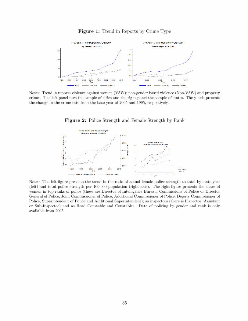
Figure 1: Trend in Reports by Crime Type

Notes: Trend in reports violence against women (VAW); non-gender based violence (Non-VAW) and propertycrimes. The left-panel uses the sample of cities and the right-panel the sample of states. The y-axis presentsthe change in the crime rate from the base year of 2005 and 1995, respectively.

Figure 2: Police Strength and Female Strength by Rank

Notes: The left figure presents the trend in the ratio of actual female police strength to total by state-year(left) and total police strength per 100,000 population (right axis). The right-figure presents the share ofwomen in top ranks of police (these are Director of Intelligence Bureau, Commissions of Police or DirectorGeneral of Police, Joint Commissioner of Police, Additional Commissioner of Police, Deputy Commissioner ofPolice, Superintendent of Police and Additional Superintendent); as inspectors (there is Inspector, Assistantor Sub-Inspector) and as Head Constable and Constables. Data of policing by gender and rank is onlyavailable from 2005.

35

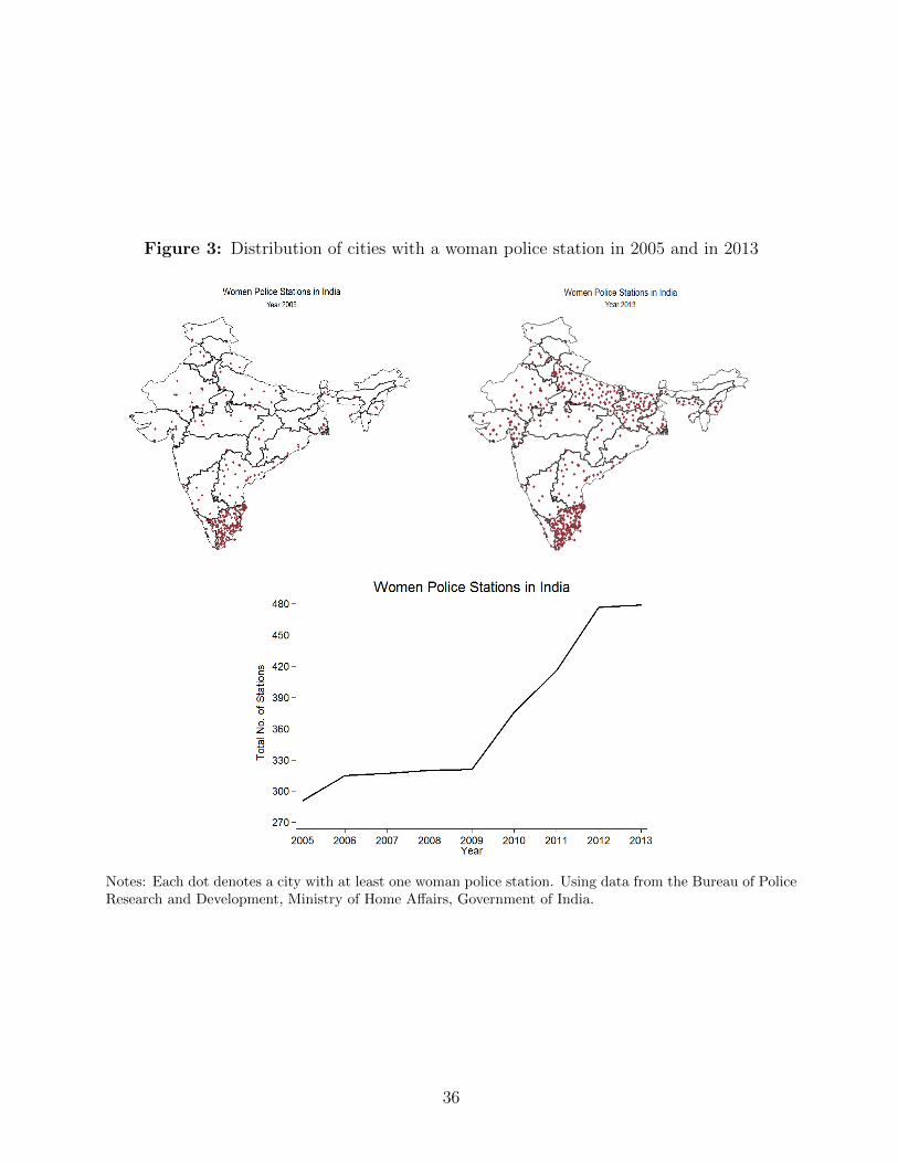
Figure 3: Distribution of cities with a woman police station in 2005 and in 2013

Notes: Each dot denotes a city with at least one woman police station. Using data from the Bureau of PoliceResearch and Development, Ministry of Home Affairs, Government of India.

36

Fig

ure

4:

Cor

rela

tion

bet

wee

nth

eye

arof

WP

San

dth

eye

arin

whic

hw

omen

firs

ten

tere

dth

ep

olic

e

AP

AS

BH

GJ

KRN

KR

MP

OR

PJ

RJ

TN

UP

WB

1940

1950

1960

1970

1980

Women's Incorporation in the Police (Year)

1970

1980

1990

2000

2010

Wom

en P

olice

Sta

tion

Polic

y In

itiatio

n

WPS

Pol

icy Y

ear

Fitte

d va

lues

Wom

en E

nter

ing

the

Polic

e an

d W

PS P

olicy

Not

es:

Th

eve

rtic

alax

isis

the

yea

rin

wh

ich

wom

enfi

rst

ente

red

the

poli

cean

dth

eh

ori

zonta

laxis

the

year

inw

hic

hth

eW

om

enP

oli

ceS

tati

on

sp

oli

cyw

asin

trod

uce

din

ast

ate.

Th

est

ates

ofM

ahar

ash

tra,

Him

ach

al

Pra

des

han

dH

ary

an

ad

idn

ot

imp

lem

ent

WP

Sb

etw

een

the

per

iod

of

1988-2

013

an

dar

en

otin

clu

ded

inth

isco

rrel

atio

n.

InA

pp

end

ixw

ep

rovid

eth

eta

ble

wit

hth

eco

mp

lete

list

of

date

sof

wom

enen

tere

ing

the

poli

ce.

37

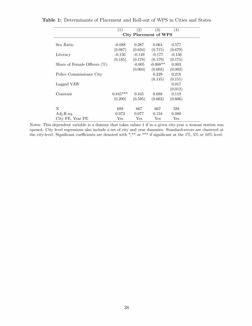
Table 1: Determinants of Placement and Roll-out of WPS in Cities and States

(1) (2) (3) (4)City Placement of WPS

Sex Ratio -0.088 0.387 0.064 0.577(0.087) (0.634) (0.715) (0.679)

Literacy -0.150 -0.149 -0.177 -0.136(0.185) (0.178) (0.179) (0.175)

Share of Female Officers (%) -0.005 -0.008** 0.003(0.004) (0.003) (0.003)

Police Commissioner City 0.229 0.218(0.145) (0.151)

Lagged VAW 0.017(0.012)

Constant 0.845*** 0.445 0.688 0.119(0.200) (0.595) (0.663) (0.606)

N 689 667 667 588Adj.R-sq. 0.073 0.077 0.134 0.080City FE, Year FE Yes Yes Yes Yes

Notes: This dependent variable is a dummy that takes values 1 if in a given city-year a woman station wasopened. City level regressions also include a set of city and year dummies. Standard-errors are clustered atthe city-level. Significant coefficients are denoted with *,** or *** if significant at the 1%, 5% or 10% level.

38

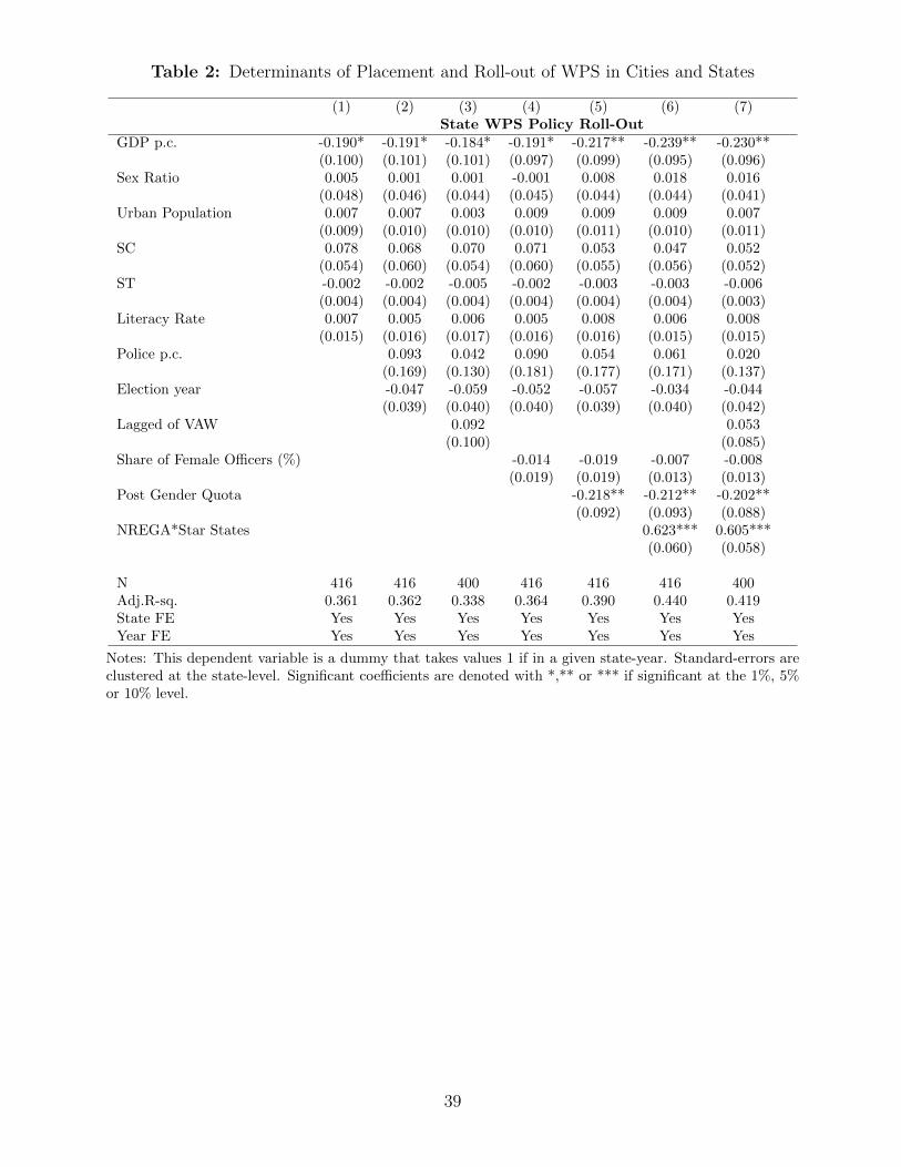
Table 2: Determinants of Placement and Roll-out of WPS in Cities and States

(1) (2) (3) (4) (5) (6) (7)State WPS Policy Roll-Out

GDP p.c. -0.190* -0.191* -0.184* -0.191* -0.217** -0.239** -0.230**(0.100) (0.101) (0.101) (0.097) (0.099) (0.095) (0.096)

Sex Ratio 0.005 0.001 0.001 -0.001 0.008 0.018 0.016(0.048) (0.046) (0.044) (0.045) (0.044) (0.044) (0.041)

Urban Population 0.007 0.007 0.003 0.009 0.009 0.009 0.007(0.009) (0.010) (0.010) (0.010) (0.011) (0.010) (0.011)

SC 0.078 0.068 0.070 0.071 0.053 0.047 0.052(0.054) (0.060) (0.054) (0.060) (0.055) (0.056) (0.052)

ST -0.002 -0.002 -0.005 -0.002 -0.003 -0.003 -0.006(0.004) (0.004) (0.004) (0.004) (0.004) (0.004) (0.003)

Literacy Rate 0.007 0.005 0.006 0.005 0.008 0.006 0.008(0.015) (0.016) (0.017) (0.016) (0.016) (0.015) (0.015)

Police p.c. 0.093 0.042 0.090 0.054 0.061 0.020(0.169) (0.130) (0.181) (0.177) (0.171) (0.137)

Election year -0.047 -0.059 -0.052 -0.057 -0.034 -0.044(0.039) (0.040) (0.040) (0.039) (0.040) (0.042)

Lagged of VAW 0.092 0.053(0.100) (0.085)

Share of Female Officers (%) -0.014 -0.019 -0.007 -0.008(0.019) (0.019) (0.013) (0.013)

Post Gender Quota -0.218** -0.212** -0.202**(0.092) (0.093) (0.088)

NREGA*Star States 0.623*** 0.605***(0.060) (0.058)

N 416 416 400 416 416 416 400Adj.R-sq. 0.361 0.362 0.338 0.364 0.390 0.440 0.419State FE Yes Yes Yes Yes Yes Yes YesYear FE Yes Yes Yes Yes Yes Yes Yes

Notes: This dependent variable is a dummy that takes values 1 if in a given state-year. Standard-errors areclustered at the state-level. Significant coefficients are denoted with *,** or *** if significant at the 1%, 5%or 10% level.

39

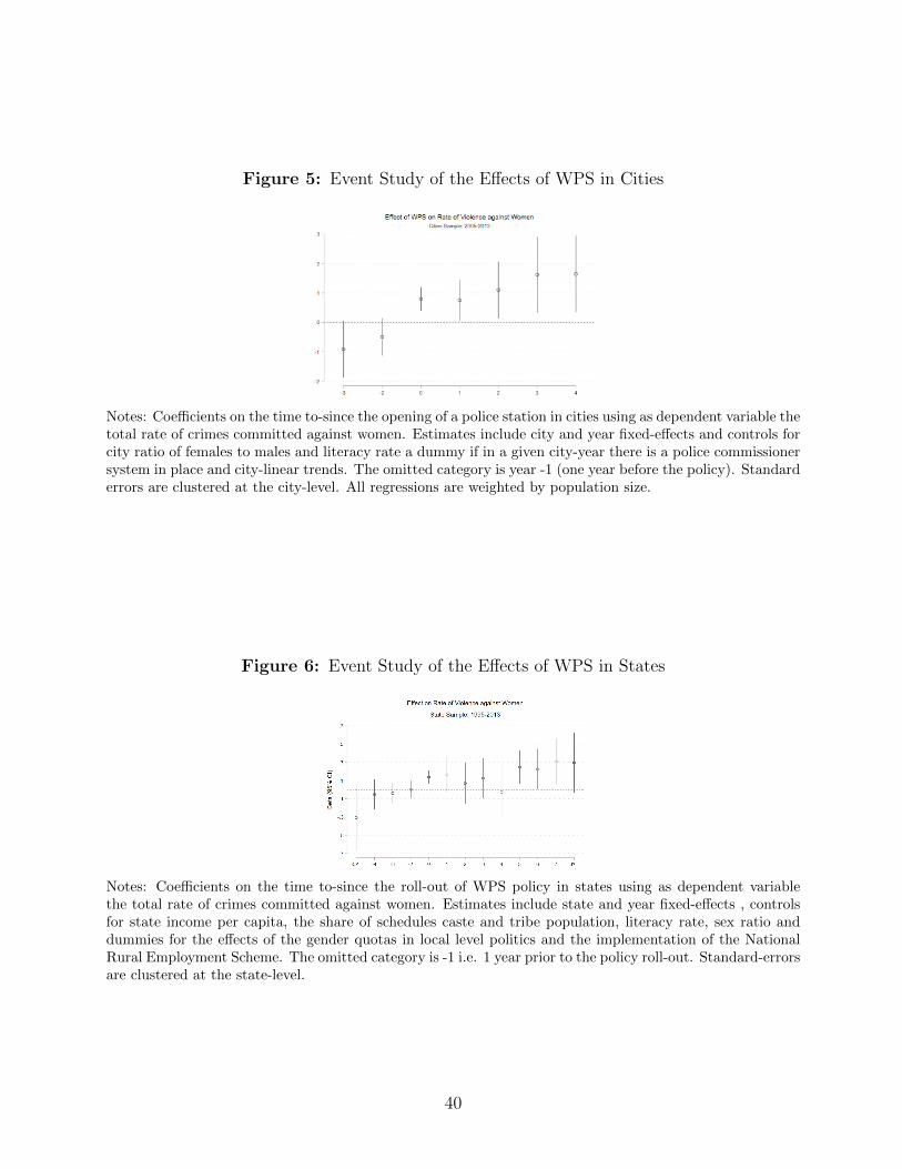
Figure 5: Event Study of the Effects of WPS in Cities

Notes: Coefficients on the time to-since the opening of a police station in cities using as dependent variable thetotal rate of crimes committed against women. Estimates include city and year fixed-effects and controls forcity ratio of females to males and literacy rate a dummy if in a given city-year there is a police commissionersystem in place and city-linear trends. The omitted category is year -1 (one year before the policy). Standarderrors are clustered at the city-level. All regressions are weighted by population size.

Figure 6: Event Study of the Effects of WPS in States

Notes: Coefficients on the time to-since the roll-out of WPS policy in states using as dependent variablethe total rate of crimes committed against women. Estimates include state and year fixed-effects , controlsfor state income per capita, the share of schedules caste and tribe population, literacy rate, sex ratio anddummies for the effects of the gender quotas in local level politics and the implementation of the NationalRural Employment Scheme. The omitted category is -1 i.e. 1 year prior to the policy roll-out. Standard-errorsare clustered at the state-level.

40

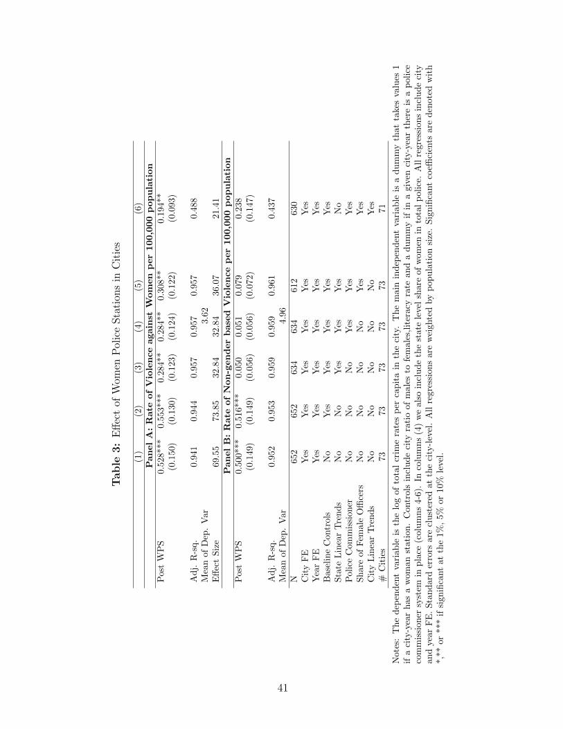
Table

3:

Eff

ect

ofW

omen

Pol

ice

Sta

tion

sin

Cit

ies

(1)

(2)

(3)

(4)

(5)

(6)

Pan

el

A:

Rate

of

Vio

len

ce

again

stW

om

en

per

100,0

00

pop

ula

tion

Pos

tW

PS

0.528***

0.5

53***

0.2

84**

0.2

84**

0.3

08**

0.1

94**

(0.1

50)

(0.1

30)

(0.1

23)

(0.1

24)

(0.1

22)

(0.0

93)

Ad

j.R

-sq.

0.9

41

0.9

44

0.9

57

0.9

57

0.9

57

0.4

88

Mea

nof

Dep

.V

ar3.6

2E

ffec

tS

ize

69.5

573.8

532.8

432.8

436.0

721.4

1P

an

el

B:

Rate

of

Non

-gen

der

base

dV

iole

nce

per

100,0

00

pop

ula

tion

Pos

tW

PS

0.500***

0.5

16***

0.0

50

0.0

51

0.0

79

0.2

38

(0.1

49)

(0.1

49)

(0.0

56)

(0.0

56)

(0.0

72)

(0.1

47)

Ad

j.R

-sq.

0.9

52

0.9

53

0.9

59

0.9

59

0.9

61

0.4

37

Mea

nof

Dep

.V

ar4.9

6N

652

652

634

634

612

630

Cit

yF

EY

esY

esY

esY

esY

esY

esY

ear

FE

Yes

Yes

Yes

Yes

Yes

Yes

Bas

elin

eC

ontr

ols

No

Yes

Yes

Yes

Yes

Yes

Sta

teL

inea

rT

ren

ds

No

No

Yes

Yes

Yes

No

Pol

ice

Com

mis

sion

erN

oN

oN

oY

esY

esY

esS

har

eof

Fem

ale

Offi

cers

No

No

No

No

Yes

Yes

Cit

yL

inea

rT

rend

sN

oN

oN

oN

oN

oY

es#

Cit

ies

73

73

73

73

73

71

Not

es:

Th

ed

epen

den

tva

riab

leis

the

log

ofto

tal

crim

era

tes

per

cap

ita

inth

eci

ty.

Th

em

ain

indep

end

ent

vari

ab

leis

ad

um

my

that

takes

valu

es1

ifa

city

-yea

rh

asa

wom

anst

atio

n.

Con

trol

sin

clu

de

city

rati

oof

male

sto

fem

ale

s,li

tera

cyra

tean

da

du

mm

yif

ina

giv

enci

ty-y

ear

ther

eis

ap

oli

ceco

mm

issi

oner

syst

emin

pla

ce(c

olu

mn

s4-

6).

Inco

lum

ns

(4)

we

als

oin

clu

de

the

state

leve

lsh

are

of

wom

enin

tota

lp

oli

ce.

All

regre

ssio

ns

incl

ud

eci

tyan

dyea

rF

E.

Sta

nd

ard

erro

rsar

ecl

ust

ered

atth

eci

ty-l

evel

.A

llre

gre

ssio

ns

are

wei

ghte

dby

pop

ula

tion

size

.S

ign

ifica

nt

coeffi

cien

tsare

den

ote

dw

ith

*,**

or**

*if

sign

ifica

nt

atth

e1%

,5%

or10

%le

vel.

41

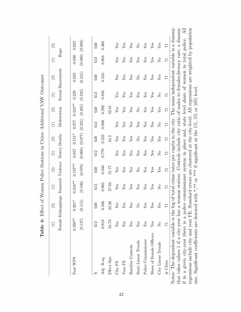
Table

4:

Eff

ect

ofW

omen

Pol

ice

Sta

tion

sin

Cit

ies-

Addit

ional

VA

WO

utc

omes

(1)

(2)

(1)

(2)

(1)

(2)

(1)

(2)

(1)

(2)

(1)

(2)

Fem

ale

Kid

nap

pin

gs

Dom

esti

cV

iole

nce

Dow

ryD

eath

sM

ole

stati

on

Sex

ual

Hara

ssm

ent

Rap

e

Pos

tW

PS

0.29

8**

0.20

1*0.2

44**

0.1

97**

0.0

27

0.1

51*

0.2

77

0.4

24**

0.2

29

0.0

33

-0.0

30

0.0

22

(0.1

27)

(0.1

15)

(0.1

06)

(0.0

78)

(0.0

60)

(0.0

77)

(0.2

31)

(0.2

01)

(0.2

35)

(0.2

41)

(0.0

80)

(0.0

88)

N61

263

0612

630

612

630

612

630

612

630

612

630

Ad

j.R

-sq.

0.91

30.

506

0.9

05

0.3

46

0.7

79

0.2

25

0.8

06

0.2

92

0.8

38

0.5

23

0.8

64

0.3

60

Eff

ect

Siz

e34

.73

22.2

627.6

321.7

716.3

52.8

1

Cit

yF

EY

esY

esY

esY

esY

esY

esY

esY

esY

esY

esY

esY

es

Yea

rF

EY

esY

esY

esY

esY

esY

esY

esY

esY

esY

esY

esY

es

Bas

elin

eC

ontr

ols

Yes

Yes

Yes

Yes

Yes

Yes

Yes

Yes

Yes

Yes

Yes

Yes

Sta

teL

inea

rT

ren

ds

Yes

No

Yes

No

Yes

No

Yes

No

Yes

No

Yes

No

Pol

ice

Com

mis

sion

erY

esY

esY

esY

esY

esY

esY

esY

esY

esY

esY

esY

es

Sh

are

ofF

emal

eO

ffice

rsY

esY

esY

esY

esY

esY

esY

esY

esY

esY

esY

esY

es

Cit

yL

inea

rT

ren

ds

No

Yes

No

Yes

No

Yes

No

Yes

No

Yes

No

Yes

#C

itie

s71

7171

71

71

71

71

7171

71

71

71

Not

es:

The

dep

enden

tva

riab

leis

the

log

ofto

tal

crim

era

tes

per

capit

ain

the

city

.T

he

mai

nin

dep

enden

tva

riab

leis

adum

my

that

take

sva

lues

1if

aci

ty-y

ear

has

aw

oman

stat

ion.

Con

trol

sin

clude

city

rati

oof

mal

esto

fem

ales

,lit

erac

yra

te;

adum

my

ifin

agi

ven

city

-yea

rth

ere

isa

pol

ice

com

mis

sion

ersy

stem

inpla

cean

d,

stat

ele

vel

shar

eof

wom

enin

tota

lp

olic

e.A

llre

gres

sion

sin

clude

city

and

year

FE

.Sta

ndar

der

rors

are

clust

ered

atth

eci

ty-l

evel

.A

llre

gres

sion

sar

ew

eigh

ted

by

pop

ula

tion

size

.Sig

nifi

cant

coeffi

cien

tsar

eden

oted

wit

h*,

**or

***

ifsi

gnifi

cant

atth

e1%

,5%

or10

%le

vel.

42

Table

5:

Eff

ect

ofW

omen

Pol

ice

Sta

tion

sin

Cit

ies-

Pre

Tre

nds

Tes

t

VA

WF

emale

Kid

nap

pin

gs

Dom

esti

cV

iole

nce

Dow

ryD

eath

sM

ole

stati

on

Sex

ual

Hara

ssm

ent

Rap

e

Pos

tW

PS

0.41

2**

0.3

70**

0.3

47**

0.2

90*

0.2

62

0.2

53

0.0

72

(0.1

90)

(0.1

62)

(0.1

54)

(0.1

49)

(0.2

42)

(0.1

90)

(0.2

02)

Pre

(On

eY

ear)

0.27

60.3

02*

0.1

73

0.1

18

-0.1

77

0.1

19

0.0

88

(0.1

91)

(0.1

72)

(0.1

39)

(0.1

10)

(0.2

11)

(0.1

81)

(0.1

64)

Pre

(Tw

oY

ears

)0.

029

-0.1

60

0.0

53

0.1

38**

-0.0

81

0.3

58***

-0.0

46

(0.0

77)

(0.1

08)

(0.0

73)

(0.0

62)

(0.0

90)

(0.1

20)

(0.0

80)

N63

0630

630

630

630

630

630

Ad

j.R

-sq.

0.48

80.5

12

0.3

45

0.2

23

0.2

90

0.5

24

0.3

58

Cit

yF

EY

esY

esY

esY

esY

esY

esY

es

Yea

rF

EY

esY

esY

esY

esY

esY

esY

es

Bas

elin

eC

ontr

ols

Yes

Yes

Yes

Yes

Yes

Yes

Yes

Pol

ice

Com

mis

sion

erY

esY

esY

esY

esY

esY

esY

es

Sh

are

ofF

emal

eO

ffice

rsY

esY

esY

esY

esY

esY

esY

es

Cit

yL

inea

rT

ren

ds

Yes

Yes

Yes

Yes

Yes

Yes

Yes

Not

es:

Th

edep

end

ent

vari

able

isth

elo

gof

tota

lcr

ime

rate

sp

erca

pit

ain

the

city

.T

he

main

ind

epen

den

tva

riab

leis

ad

um

my

that

take

sva

lues

1if

aci

ty-y

ear

has

aw

oman

stat

ion

.C

ontr

ols

incl

ud

eci

tyra

tio

of

male

sto

fem

ale

s,li

tera

cyra

te;

ad

um

my

ifin

agiv

enci

ty-y

ear

ther

eis

ap

oli

ceco

mm

issi

oner

syst

emin

pla

cean

d,

stat

ele

vel

share

of

wom

enin

tota

lp

oli

ce.

All

regre

ssio

ns

incl

ud

eci

tyan

dye

ar

FE

.Sta

nd

ard

erro

rsare

clu

ster

edat

the

city

-lev

el.

All

regr

essi

ons

are

wei

ghte

dby

pop

ula

tion

size

.P

re(O

ne

Yea

r)an

dP

re(T

wo

Yea

rs)

are

du

mm

yva

riab

les

that

take

valu

e1

ifit

ison

eye

ar/t

wo

year

sb

efor

eth

eim

ple

men

tati

onof

aW

PS

inci

ties

.S

ign

ifica

nt

coeffi

cien

tsare

den

ote

dw

ith

*,*

*or

***

ifsi

gn

ifica

nt

at

the

1%

,5%

or

10%

level

.

43

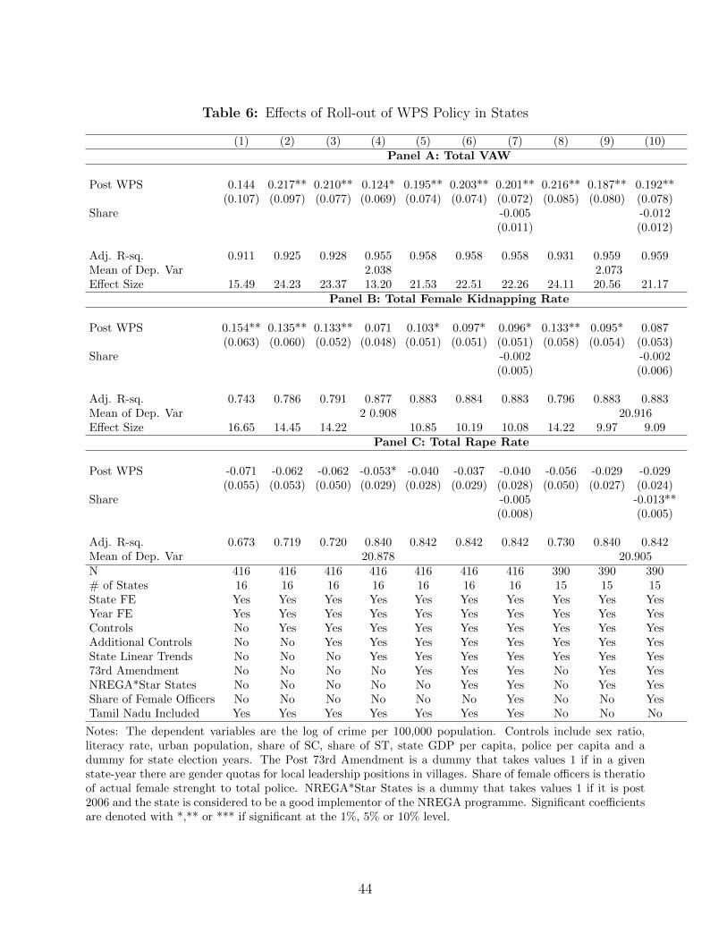
Table 6: Effects of Roll-out of WPS Policy in States

(1) (2) (3) (4) (5) (6) (7) (8) (9) (10)Panel A: Total VAW

Post WPS 0.144 0.217** 0.210** 0.124* 0.195** 0.203** 0.201** 0.216** 0.187** 0.192**(0.107) (0.097) (0.077) (0.069) (0.074) (0.074) (0.072) (0.085) (0.080) (0.078)

Share -0.005 -0.012(0.011) (0.012)

Adj. R-sq. 0.911 0.925 0.928 0.955 0.958 0.958 0.958 0.931 0.959 0.959Mean of Dep. Var 2.038 2.073Effect Size 15.49 24.23 23.37 13.20 21.53 22.51 22.26 24.11 20.56 21.17

Panel B: Total Female Kidnapping Rate

Post WPS 0.154** 0.135** 0.133** 0.071 0.103* 0.097* 0.096* 0.133** 0.095* 0.087(0.063) (0.060) (0.052) (0.048) (0.051) (0.051) (0.051) (0.058) (0.054) (0.053)

Share -0.002 -0.002(0.005) (0.006)

Adj. R-sq. 0.743 0.786 0.791 0.877 0.883 0.884 0.883 0.796 0.883 0.883Mean of Dep. Var 2 0.908 20.916Effect Size 16.65 14.45 14.22 10.85 10.19 10.08 14.22 9.97 9.09

Panel C: Total Rape Rate

Post WPS -0.071 -0.062 -0.062 -0.053* -0.040 -0.037 -0.040 -0.056 -0.029 -0.029(0.055) (0.053) (0.050) (0.029) (0.028) (0.029) (0.028) (0.050) (0.027) (0.024)

Share -0.005 -0.013**(0.008) (0.005)

Adj. R-sq. 0.673 0.719 0.720 0.840 0.842 0.842 0.842 0.730 0.840 0.842Mean of Dep. Var 20.878 20.905N 416 416 416 416 416 416 416 390 390 390# of States 16 16 16 16 16 16 16 15 15 15State FE Yes Yes Yes Yes Yes Yes Yes Yes Yes YesYear FE Yes Yes Yes Yes Yes Yes Yes Yes Yes YesControls No Yes Yes Yes Yes Yes Yes Yes Yes YesAdditional Controls No No Yes Yes Yes Yes Yes Yes Yes YesState Linear Trends No No No Yes Yes Yes Yes Yes Yes Yes73rd Amendment No No No No Yes Yes Yes No Yes YesNREGA*Star States No No No No No Yes Yes No Yes YesShare of Female Officers No No No No No No Yes No No YesTamil Nadu Included Yes Yes Yes Yes Yes Yes Yes No No No

Notes: The dependent variables are the log of crime per 100,000 population. Controls include sex ratio,literacy rate, urban population, share of SC, share of ST, state GDP per capita, police per capita and adummy for state election years. The Post 73rd Amendment is a dummy that takes values 1 if in a givenstate-year there are gender quotas for local leadership positions in villages. Share of female officers is theratioof actual female strenght to total police. NREGA*Star States is a dummy that takes values 1 if it is post2006 and the state is considered to be a good implementor of the NREGA programme. Significant coefficientsare denoted with *,** or *** if significant at the 1%, 5% or 10% level.

44

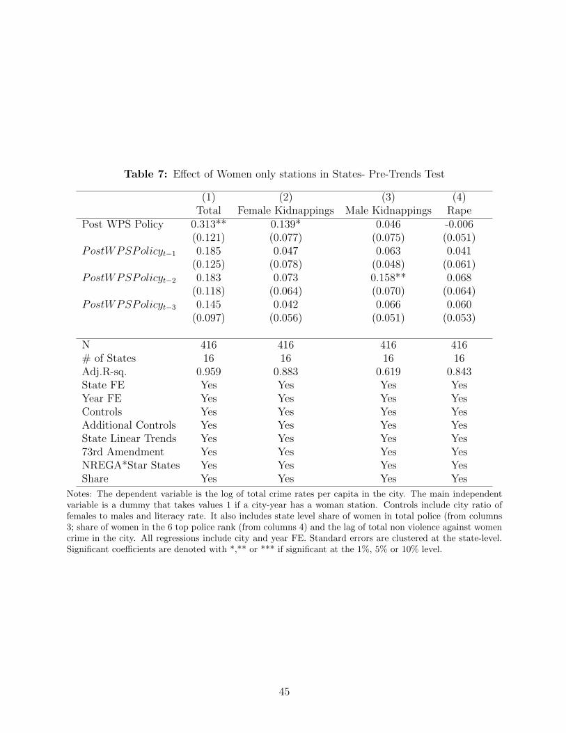
Table 7: Effect of Women only stations in States- Pre-Trends Test

(1) (2) (3) (4)Total Female Kidnappings Male Kidnappings Rape

Post WPS Policy 0.313** 0.139* 0.046 -0.006(0.121) (0.077) (0.075) (0.051)

PostWPSPolicyt−1 0.185 0.047 0.063 0.041(0.125) (0.078) (0.048) (0.061)

PostWPSPolicyt−2 0.183 0.073 0.158** 0.068(0.118) (0.064) (0.070) (0.064)

PostWPSPolicyt−3 0.145 0.042 0.066 0.060(0.097) (0.056) (0.051) (0.053)

N 416 416 416 416# of States 16 16 16 16Adj.R-sq. 0.959 0.883 0.619 0.843State FE Yes Yes Yes YesYear FE Yes Yes Yes YesControls Yes Yes Yes YesAdditional Controls Yes Yes Yes YesState Linear Trends Yes Yes Yes Yes73rd Amendment Yes Yes Yes YesNREGA*Star States Yes Yes Yes YesShare Yes Yes Yes Yes

Notes: The dependent variable is the log of total crime rates per capita in the city. The main independentvariable is a dummy that takes values 1 if a city-year has a woman station. Controls include city ratio offemales to males and literacy rate. It also includes state level share of women in total police (from columns3; share of women in the 6 top police rank (from columns 4) and the lag of total non violence against womencrime in the city. All regressions include city and year FE. Standard errors are clustered at the state-level.Significant coefficients are denoted with *,** or *** if significant at the 1%, 5% or 10% level.

45

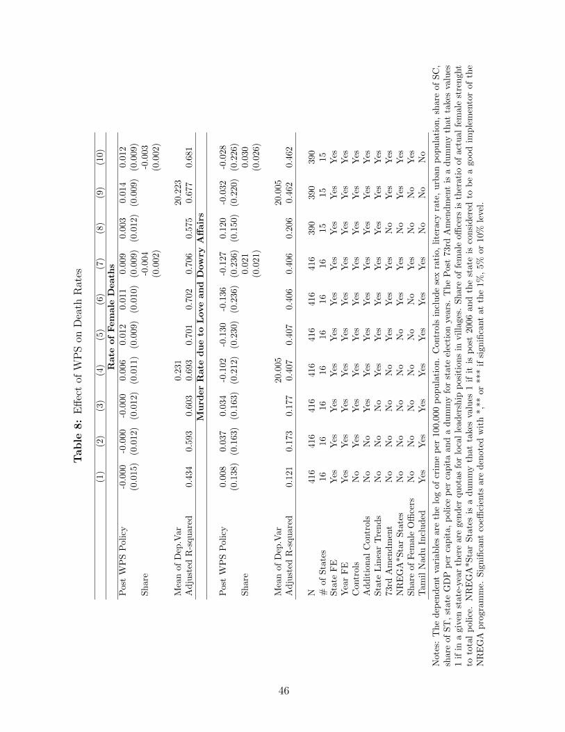
Table

8:

Eff

ect

ofW

PS

onD

eath

Rat

es

(1)

(2)

(3)

(4)

(5)

(6)

(7)

(8)

(9)

(10)

Rate

of

Fem

ale

Death

sP

ost

WP

SP

olic

y-0

.000

-0.0

00

-0.0

00

0.0

06

0.0

12

0.0

11

0.0

09

0.0

03

0.0

14

0.0

12

(0.0

15)

(0.0

12)

(0.0

12)

(0.0

11)

(0.0

09)

(0.0

10)

(0.0

09)

(0.0

12)

(0.0

09)

(0.0

09)

Sh

are

-0.0

04

-0.0

03

(0.0

02)

(0.0

02)

Mea

nof

Dep

.Var

0.2

31

20.2

23

Ad

just

edR

-squ

ared

0.43

40.5

93

0.6

03

0.6

93

0.7

01

0.7

02

0.7

060.5

75

0.6

77

0.6

81

Mu

rder

Rate

du

eto

Love

an

dD

ow

ryA

ffair

s

Pos

tW

PS

Pol

icy

0.00

80.0

37

0.0

34

-0.1

02

-0.1

30

-0.1

36

-0.1

270.1

20

-0.0

32

-0.0

28

(0.1

38)

(0.1

63)

(0.1

63)

(0.2

12)

(0.2

30)

(0.2

36)

(0.2

36)

(0.1

50)

(0.2

20)

(0.2

26)

Sh

are

0.0

210.0

30

(0.0

21)

(0.0

26)

Mea

nof

Dep

.Var

20.0

05

20.0

05

Ad

just

edR

-squ

ared

0.12

10.1

73

0.1

77

0.4

07

0.4

07

0.4

06

0.4

060.2

06

0.4

62

0.4

62

N41

6416

416

416

416

416

416

390

390

390

#of

Sta

tes

1616

16

16

16

16

16

15

15

15

Sta

teF

EY

esY

esY

esY

esY

esY

esY

esY

esY

esY

esY

ear

FE

Yes

Yes

Yes

Yes

Yes

Yes

Yes

Yes

Yes

Yes

Con

trol

sN

oY

esY

esY

esY

esY

esY

esY

esY

esY

esA

dd

itio

nal

Con

trol

sN

oN

oY

esY

esY

esY

esY

esY

esY

esY

esS

tate

Lin

ear

Tre

nd

sN

oN

oN

oY

esY

esY

esY

esY

esY

esY

es73

rdA

men

dm

ent

No

No

No

No

Yes

Yes

Yes

No

Yes

Yes

NR

EG

A*S

tar

Sta

tes

No

No

No

No

No

Yes

Yes

No

Yes

Yes

Sh

are

ofF

emal

eO

ffice

rsN

oN

oN

oN

oN

oN

oY

esN

oN

oY

esT

amil

Nad

uIn

clu

ded

Yes

Yes

Yes

Yes

Yes

Yes

Yes

No

No

No

Not

es:

Th

ed

epen

den

tva

riab

les

are

the

log

ofcr

ime

per

100,0

00

pop

ula

tion

.C

ontr

ols

incl

ud

ese

xra

tio,

lite

racy

rate

,u

rban

pop

ula

tion

,sh

are

of

SC

,sh

are

ofS

T,

stat

eG

DP

per

cap

ita,

pol

ice

per

cap

ita

an

da

du

mm

yfo

rst

ate

elec

tion

years

.T

he

Post

73rd

Am

end

men

tis

ad

um

my

that

takes

valu

es1

ifin

agi

ven

stat

e-ye

arth

ere

are

gen

der

qu

otas

for

loca

lle

ad

ersh

ipp

osi

tion

sin

vil

lages

.S

hare

of

fem

ale

offi

cers

isth

erati

oof

act

ual

fem

ale

stre

nght

toto

tal

pol

ice.

NR

EG

A*S

tar

Sta

tes

isa

du

mm

yth

at

take

sva

lues

1if

itis

post

2006

an

dth

est

ate

isco

nsi

der

edto

be

agood

imp

lem

ento

rof

the

NR

EG

Ap

rogr

amm

e.S

ign

ifica

nt

coeffi

cien

tsar

ed

enote

dw

ith

*,*

*or

***

ifsi

gn

ifica

nt

at

the

1%

,5%

or

10%

level

.

46

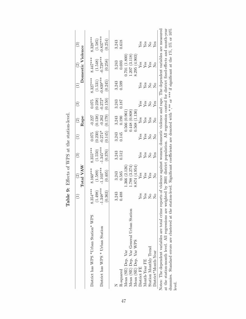
Table

9:

Eff

ects

ofW

PS

atth

est

atio

n-l

evel

.

(1)

(2)

(3)

(1)

(2)

(3)

(1)

(2)

(3)

Tota

lV

AW

Rap

eD

om

est

icV

iole

nce

Dis

tric

th

asW

PS

*Urb

anS

tati

on*

WP

S8.3

54***

8.1

60***

8.3

55***

0.0

75

-0.2

27

0.0

75

8.3

27***

8.4

47***

8.3

28***

(1.4

98)

(1.5

89)

(1.5

50)

(0.2

30)

(0.1

38)

(0.2

38)

(1.5

31)

(1.5

48)

(1.5

85)

Dis

tric

th

asW

PS

*U

rban

Sta

tion

-1.3

48***

-1.1

03***

-1.3

45***

-0.2

74*

-0.2

62

-0.2

72*

-0.8

39***

-0.7

29***

-0.8

37***

(0.3

63)

(0.4

05)

(0.3

76)

(0.1

45)

(0.1

79)

(0.1

50)

(0.2

45)

(0.2

58)

(0.2

54)

N3,2

43

3,2

43

3,2

43

3,2

43

3,2

43

3,2

43

3,2

43

3,2

43

3,2

43

R-s

qu

ared

0.4

88

0.5

85

0.5

12

0.1

45

0.1

90

0.1

87

0.5

99

0.6

93

0.6

18

Mea

n(S

E)

Dep

.V

ar1.3

66

(2.1

26)

0.5

66

(0.9

61)

0.7

01

(1.8

00)

Mea

n(S

E)

Dep

.V

arG

ener

alU

rban

Sta

tion

1.7

88

(3.2

74)

0.4

48

(0.8

08)

1.2

07

(3.1

18)

Mea

n(S

E)

Dep

.V

arW

PS

8.8

74

(4.9

54)

0.5

68

(1.1

36)

8.2

95

(4.9

03)

Dis

tric

tF

EY

esY

esY

esY

esY

esY

esY

esY

esY

esM

onth

-Yea

rF

EY

esY

esY

esY

esY

esY

esY

esY

esY

esS

tati

onM

onth

lyT

ren

dN

oY

esN

oN

oY

esN

oN

oY

esN

oD

istr

ict*

Mon

th-Y

ear

No

No

Yes

No

No

Yes

No

No

Yes

Not

es:

Th

ed

epen

den

tva

riab

les

are

tota

lcr

ime

rep

ort

sof

vio

len

ceagain

stw

om

en;

dom

esti

cvio

len

cean

dra

pe.

Th

ed

epen

den

tva

riab

les

are

mea

sure

dat

the

stat

ion

-mon

thle

vel.

All

regr

essi

ons

are

wei

ghte

dby

2001

dis

tric

tp

op

ula

tion.

All

regre

ssio

nco

ntr

ol

for

dis

tric

tfi

xed

-eff

ects

an

dm

onth

-yea

rd

um

mie

s.S

tan

dar

der

rors

are

clu

ster

edat

the

stati

on

-lev

el.

Sig

nifi

cant

coeffi

cien

tsare

den

ote

dw

ith

*,*

*or

***

ifsi

gn

ifica

nt

at

the

1%

,5%

or

10%

leve

l.

47

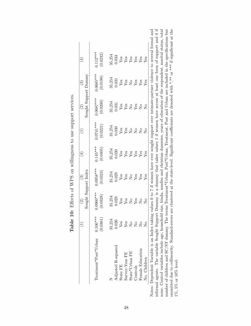
Table

10:

Eff

ects

ofW

PS

onw

illingn

ess

touse

supp

ort

serv

ices

.

(1)

(2)

(3)

(4)

(1)

(2)

(3)

(4)

Sou

ght

Su

pp

ort

Ind

exS

ought

Su

pp

ort

Dum

my

Tre

atm

ent*

Pos

t*U

rban

0.10

6***

0.0

960***

0.0

958***

0.1

45***

0.0

741***

0.0

687***

0.0

685***

0.1

12***

(0.0

361)

(0.0

328)

(0.0

324)

(0.0

405)

(0.0

221)

(0.0

200)

(0.0

198)

(0.0

232)

N35

,254

35,2

54

35,2

54

35,2

54

35,2

54

35,2

54

35,2

54

35,2

54

Ad

just

edR

-squ

ared

0.02

60.0

29

0.0

29

0.0

30

0.0

30

0.0

31

0.0

31

0.0

33

Sta

teF

EY

esY

esY

esY

esY

esY

esY

esY

esS

urv

ey-Y

ear

FE

Yes

Yes

Yes

Yes

Yes

Yes

Yes

Yes

Sta

te*U

rban

FE

No

No

No

Yes

No

No

No

Yes

Con

trol

sN

oY

esY

esY

esN

oY

esY

esY

esF

emal

eE

du

cati

onN

oN

oY

esY

esN

oN

oY

esY

esN

o.C

hil

dre

nN

oN

oY

esY

esN

oN

oY

esY

es

Not

es:

Dep

end

ent

Var

iab

leis

anIn

dex

takin

gva

lues

0to

7if

wom

enh

ave

ever

sou

ght

sup

port

over

inti

mate

-part

ner

vio

len

ceto

seve

ral

form

al

an

din

form

alag

ents

.T

he

vari

able

Sou

ght

Su

pp

ort

Du

mm

yis

ad

um

my

that

take

sva

lues

1if

wom

enh

ave

acc

ess

at

least

on

efo

rmof

sup

port

an

d0

ifn

one.

Con

trol

vari

able

sin

clu

de

age,

hou

seh

old

size

,h

ind

u,

mu

slim

an

dch

rist

ian

du

mm

ies,

years

of

edu

cati

on

of

the

resp

on

den

t,m

ari

tal

statu

s,to

tal

nu

mb

erof

chil

dre

nan

dS

C/S

Td

um

my.

The

term

sT

reatm

ent*

Urb

an

,P

ost

*U

rban

,T

reatm

ent,

Post

and

Urb

an

are

incl

ud

edin

the

spec

ifica

tion

sb

ut

omm

itte

dd

ue

toco

llin

eari

ty.

Sta

nd

ard

-err

ors

are

clu

ster

edat

the

state

-lev

el.

Sig

nifi

cant

coeffi

cien

tsar

ed

enote

dw

ith

*,*

*or

***

ifsi

gn

ifica

nt

at

the

1%,

5%or

10%

level

.

48

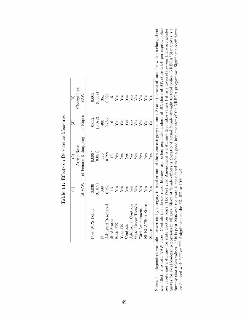
Table

11:

Eff

ects

onD

eter

rence

Mea

sure

s

(1)

(2)

(3)

(4)

Arr

est

Rate

Ch

arg

esh

eet

of

VA

Wof

Fem

ale

Kid

nap

pin

gof

Rap

esV

AW

Pos

tW

PS

Pol

icy

-0.0

30

0.0

99*

-0.0

32

-0.0

05

(0.1

09)

(0.0

51)

(0.0

72)

(0.0

37)

N399

383

400

351

Ad

just

edR

-squ

ared

0.7

95

0.7

99

0.7

86

0.0

96

#of

Sta

tes

16

16

16

16

Sta

teF

EY

esY

esY

esY

esY

ear

FE

Yes

Yes

Yes

Yes

Con

trol

sY

esY

esY

esY

esA

dd

itio

nal

Con

trols

Yes

Yes

Yes

Yes

Sta

teL

inea

rT

ren

ds

Yes

Yes

Yes

Yes

73rd

Am

end

men

tY

esY

esY

esY

esN

RE

GA

*Sta

rS

tate

sY

esY

esY

esY

esS

har

eY

esY

esY

esY

es

Not

es:

Th

ed

epen

den

tva

riab

les

are

arre

sts

by

cate

gory

toto

tal

crim

esof

the

sam

eca

tegory

(colu

mn

s3)

an

dth

era

teof

case

sfo

rw

hic

ha

charg

esh

eet

was

fill

edin

toto

tal

VA

Wca

ses.

Con

trol

sin

clu

de

sex

rati

o,

lite

racy

rate

,u

rban

pop

ula

tion

,sh

are

of

SC

,sh

are

of

ST

,st

ate

GD

Pp

erca

pit

a,

poli

cep

erca

pit

aan

da

du

mm

yfo

rst

ate

elec

tion

year

s.T

he

Post

73rd

Am

end

men

tis

ad

um

my

that

take

sva

lues

1if

ina

giv

enst

ate

-yea

rth

ere

are

gen

der

qu

otas

for

loca

lle

ader

ship

pos

itio

ns

invil

lage

s.S

hare

of

fem

ale

offi

cers

isth

erati

oof

act

ual

fem

ale

stre

nght

toto

tal

poli

ce.

NR

EG

A*S

tar

Sta

tes

isa

du

mm

yth

atta

kes

valu

es1

ifit

isp

ost

2006

and

the

state

isco

nsi

der

edto

be

agood

imp

lem

ento

rof

the

NR

EG

Ap

rogra

mm

e.S

ignifi

cant

coeffi

cien

tsar

ed

enot

edw

ith

*,**

or**

*if

sign

ifica

nt

atth

e1%

,5%

or

10%

leve

l.

49

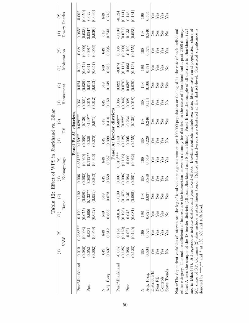
Table

12:

Eff

ect

ofW

PS

inJhar

khan

dvs.

Bih

ar(1

)(2

)(1

)(2

)(1

)(2

)(1

)(2

)(1

)(2

)(1

)(2

)(1

)(2

)V

AW

Rap

eK

idn

ap

pin

gs

DV

Hara

ssm

ent

Mole

stati

on

Dow

ryD

eath

s

Pan

el

B:

All

dis

tric

tsP

ost*

Jh

arkh

and

0.01

00.

268*

**0.

120

-0.1

02

0.0

06

0.3

51***

0.1

59**

0.6

29***

0.0

31

0.0

24

-0.1

11

-0.0

80

-0.0

65*

-0.0

02

(0.0

86)

(0.0

93)

(0.0

75)

(0.0

89)

(0.0

62)

(0.0

69)

(0.0

68)

(0.1

39)

(0.0

21)

(0.0

39)

(0.0

74)

(0.0

90)

(0.0

38)

(0.0

50)

Pos

t0.

052

-0.0

31-0

.006

0.1

33**

0.0

80*

-0.1

12**

0.0

26

-0.1

49**

0.0

15

0.0

14

0.0

41

0.0

91*

0.0

54*

0.0

22

(0.0

62)

(0.0

59)

(0.0

52)

(0.0

51)

(0.0

43)

(0.0

46)

(0.0

70)

(0.0

71)

(0.0

12)

(0.0

13)

(0.0

57)

(0.0

53)

(0.0

30)

(0.0

36)

N64

964

964

9649

649

649

649

649

649

649

649

649

649

649

Ad

j.R

-sq.

0.60

70.

612

0.65

80.6

73

0.5

59

0.5

87

0.3

99

0.4

18

0.1

50

0.1

49

0.2

83

0.2

95

0.7

43

0.7

43

Pan

el

A:

Bord

er

dis

tric

tsP

ost*

Jh

arkh

and

-0.0

870.

164

-0.0

16-0

.109

0.0

97

0.3

13***

0.1

43

0.5

89**

0.0

35

0.0

22

-0.0

74

0.0

38

-0.1

04

-0.1

24

(0.1

25)

(0.1

69)

(0.1

26)

(0.1

57)

(0.0

96)

(0.1

06)

(0.1

28)

(0.2

22)

(0.0

46)

(0.0

70)

(0.1

15)

(0.2

00)

(0.0

71)

(0.1

41)

Pos

t0.

086

-0.0

210.

045

0.1

40

0.0

84

-0.0

60

0.0

05

-0.2

34

0.0

28

0.0

39*

-0.0

63

-0.1

02

0.1

33

0.1

46

(0.1

23)

(0.1

40)

(0.0

81)

(0.0

95)

(0.0

61)

(0.0

62)

(0.1

55)

(0.1

38)

(0.0

18)

(0.0

20)

(0.1

26)

(0.1

55)

(0.0

83)

(0.1

31)

N19

819

819

8198

198

198

198

198

198

198

198

198

198

198

Ad

j.R

-sq.

0.50

40.

524

0.62

30.6

37

0.5

40

0.5

49

0.2

29

0.2

46

0.1

14

0.1

06

0.3

71

0.3

74

0.5

40

0.5

34

Dis

tric

tF

EY

esY

esY

esY

esY

esY

esY

esY

esY

esY

esY

esY

esY

esY

esY

ear

FE

Yes

Yes

Yes

Yes

Yes

Yes

Yes

Yes

Yes

Yes

Yes

Yes

Yes

Yes

Con

trol

sY

esY

esY

esY

esY

esY

esY

esY

esY

esY

esY

esY

esY

esY

esS

tate

Tre

nd

sN

oY

esN

oY

esN

oY

esN

oY

esN

oY

esN

oY

esN

oY

es

Not

es:T

he

dep

end

ent

vari

able

sof

inte

rest

are

the

log

of

tota

lvio

len

ceagain

stw

om

enp

er100,0

00

pop

ula

tion

or

the

log

of

1+

the

rate

of

each

ind

ivid

ual

crim

eca

tego

ry.

Th

em

ain

coeffi

cien

tsof

inte

rest

are

the

inte

ract

ion

bet

wee

na

du

mm

yfo

rd

istr

icts

inth

est

ate

of

Jhark

han

dand

ap

ost

2006

du

mm

y.P

anel

Au

ses

the

sam

ple

ofth

e18

bor

der

dis

tric

ts(1

0fr

om

Jh

ark

han

dan

d8

from

Bih

ar)

.P

an

elB

use

sth

esa

mp

leof

all

dis

tric

tsin

Jh

ark

han

d(2

2)

and

inB

ihar

(37)

.A

llre

gres

sion

sin

clu

de

dis

tric

tan

dye

ar

fixed

effec

ts.

Base

lin

eco

ntr

ols

incl

ud

ese

xra

tio,

lite

racy

rate

,ru

ral

pop

ula

tion

,sh

are

of

SC

,sh

are

ofS

T.

Col

um

ns

(2)

also

incl

ud

ea

state

lin

ear

tren

d.

Rob

ust

stand

ard

-err

ors

are

clu

ster

edat

the

dis

tric

t-le

vel.

Sta

tist

ical

signifi

can

ceis

den

oted

by

***,

**an

d*

at1%

,5%

and

10%

level

.

50

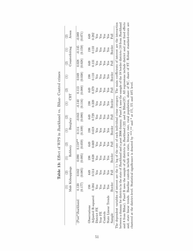
Table

13:

Eff

ect

ofW

PS

inJhar

khan

dvs.

Bih

ar-

Con

trol

crim

es

(1)

(2)

(1)

(2)

(1)

(2)

(1)

(2)

(1)

(2)

(1)

(2)

Mal

eK

idn

app

ings

Rob

ber

yB

urg

lary

CB

TC

ou

nte

rfei

tin

gA

rson

(Pos

t*Jh

arkh

and

0.12

00.

042

0.0

90

0.1

18**

0.1

14

-0.0

43

-0.1

40

0.1

130.0

49

0.0

28

-0.1

45

-0.0

89

(0.1

77)

(0.0

85)

(0.0

95)

(0.0

59)

(0.1

09)

(0.0

80)

(0.1

16)

(0.0

88)

(0.0

38)

(0.0

28)

(0.1

59)

(0.0

71)

Ob

serv

atio

ns

198

649

198

649

198

649

198

649

198

649

198

649

Ad

just

edR

-squ

ared

0.38

40.

514

0.6

38

0.6

69

0.6

18

0.7

29

0.3

39

0.3

790.1

10

0.1

31

0.1

10

0.2

82

Dis

tric

tF

EY

esY

esY

esY

esY

esY

esY

esY

esY

esY

esY

esY

esY

ear

FE

Yes

Yes

Yes

Yes

Yes

Yes

Yes

Yes

Yes

Yes

Yes

Yes

Con

trol

sY

esY

esY

esY

esY

esY

esY

esY

esY

esY

esY

esY

esS

tate

Lin

ear

Tre

nd

sY

esY

esY

esY

esY

esY

esY

esY

esY

esY

esY

esY

esS

amp

leB

order

Fu

llB

ord

erF

ull

Bord

erF

ull

Bord

erF

ull

Bord

erF

ull

Bord

erF

ull

Th

ed

epen

den

tva

riab

les

ofin

tere

star

eth

e1+

log

of

the

rate

of

each

ind

ivid

ual

crim

eca

tegory

.T

he

main

coeffi

cien

tsof

inte

rest

are

the

inte

ract

ion

bet

wee

na

du

mm

yfo

rd

istr

icts

inth

est

ate

ofJh

ark

han

dan

da

post

2006

du

mm

y.P

anel

Au

ses

the

sam

ple

of

the

18

bord

erd

istr

icts

(10

from

Jh

ark

hand

and

8fr

omB

ihar

).P

anel

Bu

ses

the

sam

ple

ofal

ld

istr

icts

inJh

ark

han

d(2

2)

an

din

Bih

ar(

37).

All

regre

ssio

ns

incl

ud

ed

istr

ict

an

dye

ar

fixed

effec

tsan

d,

stat

eli

nea

rtr

end

s.B

asel

ine

contr

ols

incl

ud

ese

xra

tio,

lite

racy

rate

,ru

ral

pop

ula

tion

,sh

are

of

SC

,sh

are

of

ST

.R

ob

ust

stan

dard

-err

ors

are

clu

ster

edat

the

dis

tric

t-le

vel.

Sta

tist

ical

sign

ifica

nce

isd

enote

dby

***,*

*an

d*

at

1%

,5%

an

d10%

leve

l.

51

Online Appendix to Gender, Crime and Punishment:

The effects of Women Police Stations in India

52

Table 14: Women in the Police and Women-only Stations by State

State Year Women Entered the Police Year WPS Implemented Share of WomenTamil Nadu 1973 1992 5.871Maharashtra 1939 0 4.244Himachal Pradesh 1966 2014 3.150Karnataka 1960 1994 3.020Kerala 1939 1973 3.015Orissa 1961 1994 2.982Rajasthan 1955 1989 2.326Gujarat 1948 1991 2.168Madhya Pradesh 1961 1987 2.111Haryana 1966 2015 2.016Punjab 1949 2010 1.981Uttar Pradesh 1967 1993 1.620Andhra Pradesh 1959 2002 1.520West Bengal 1949 2012 1.469Bihar 1952 2006 1.227Assam 1967 1993 0.491

Notes: This tables presents by state the year in which women were first employed in the law and order;the year in which WPS were implemented and the average sharee of women in the police over the period1988-2013. Note the geographic boundaries of the states are with respect to pre 2001 boundaries. Tablesorted by average share of female officers in states (column 3).

53

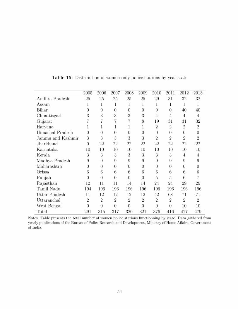
Table 15: Distribution of women-only police stations by year-state

2005 2006 2007 2008 2009 2010 2011 2012 2013Andhra Pradesh 25 25 25 25 25 29 31 32 32Assam 1 1 1 1 1 1 1 1 1Bihar 0 0 0 0 0 0 0 40 40Chhattisgarh 3 3 3 3 3 4 4 4 4Gujarat 7 7 7 7 8 19 31 31 32Haryana 1 1 1 1 1 2 2 2 2Himachal Pradesh 0 0 0 0 0 0 0 0 0Jammu and Kashmir 3 3 3 3 3 2 2 2 2Jharkhand 0 22 22 22 22 22 22 22 22Karnataka 10 10 10 10 10 10 10 10 10Kerala 3 3 3 3 3 3 3 4 4Madhya Pradesh 9 9 9 9 9 9 9 9 9Maharashtra 0 0 0 0 0 0 0 0 0Orissa 6 6 6 6 6 6 6 6 6Punjab 0 0 0 0 0 5 5 6 7Rajasthan 12 11 11 14 14 24 24 29 29Tamil Nadu 194 196 196 196 196 196 196 196 196Uttar Pradesh 11 12 12 12 12 42 68 71 71Uttaranchal 2 2 2 2 2 2 2 2 2West Bengal 0 0 0 0 0 0 0 10 10Total 291 315 317 320 321 376 416 477 479

Notes: Table presents the total number of women police stations functionning by state. Data gathered fromyearly publications of the Bureau of Police Research and Development, Ministry of Home Affairs, Governmentof India.

54

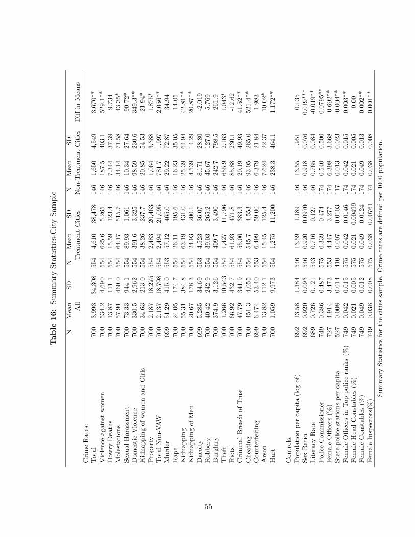
Table

16:

Sum

mar

ySta

tist

ics-

Cit

ySam

ple

NM

ean

SD

NM

ean

SD

NM

ean

SD

All

Tre

atm

ent

Cit

ies

Non

-Tre

atm

ent

Cit

ies

Diff

inM

ean

sC

rim

eR

ates

:T

otal

700

3,9

93

34,3

08

554

4,6

10

38,4

78

146

1,6

50

4,5

49

3,6

70**

Vio

len

ceag

ain

stw

omen

700

534.2

4,6

90

554

625.6

5,2

65

146

187.5

403.1

529.1

**

Dow

ryD

eath

s700

13.8

7111.1

554

15.5

9123.4

146

7.3

44

37.3

99.7

34

Mol

esta

tion

s700

57.9

1460.0

554

64.1

7515.7

146

34.1

471.5

843.3

5*

Sex

ual

Har

assm

ent

700

73.3

3944.1

554

89.9

31,0

61

146

10.3

427.6

490.7

2*

Dom

esti

cV

iole

nce

700

330.5

2,9

62

554

391.6

3,3

25

146

98.5

9230.6

349.3

**

Kid

nap

pin

gof

wom

enan

dG

irls

700

34.6

3213.0

554

38.2

6237.7

146

20.8

554.5

321.9

4*

Pro

per

ty700

2,1

87

18,2

75

554

2,4

83

20,4

63

146

1,0

64

3,3

88

1,8

75*

Tot

alN

on-V

AW

700

2,1

37

18,7

98

554

2,4

94

21,0

95

146

781.7

1,9

97

2,0

56**

Mu

rder

699

51.2

9415.0

553

57.1

2465.0

146

29.2

272.8

734.9

4R

ape

700

24.0

5174.7

554

26.1

1195.6

146

16.2

335.0

514.0

5K

idn

app

ing

700

55.3

1384.8

554

63.1

9431.0

146

25.3

964.9

442.8

1**

Kid

nap

pin

gof

Men

700

20.6

7178.3

554

24.9

3200.1

146

4.5

39

14.2

920.8

7**

Dac

oity

699

5.2

85

34.6

9553

4.5

23

36.0

7146

8.1

71

28.8

0-2

.019

Rob

ber

y700

40.4

2242.9

554

39.0

3265.2

146

45.6

7127.0

5.7

69

Bu

rgla

ry700

374.9

3,1

26

554

409.7

3,4

90

146

242.7

798.5

261.9

Th

eft

700

1,2

66

10,5

43

554

1,4

27

11,7

96

146

655.9

2,1

63

1,0

43*

Rio

ts700

66.9

2432.7

554

61.9

3471.8

146

85.8

8230.1

-12.6

2C

rim

inal

Bre

ach

ofT

rust

700

47.7

9341.9

554

55.0

6383.3

146

20.1

949.9

341.5

2**

Ch

eati

ng

700

451.3

4,0

55

554

545.7

4,5

53

146

93.0

5265.0

521.4

**

Cou

nte

rfei

tin

g699

6.4

74

53.4

0553

6.4

99

59.0

0146

6.3

79

21.8

41.9

83

Ars

on700

13.8

2112.1

554

15.4

5125.4

146

7.6

24

22.3

710.0

2*

Hu

rt700

1,0

59

9,9

73

554

1,2

75

11,2

00

146

238.3

464.1

1,1

72**

Con

trol

s:P

opu

lati

onp

erca

pit

a(l

ogof

)692

13.5

81.3

84

546

13.5

91.1

89

146

13.5

51.9

51

0.1

35

Sex

Rat

io692

0.9

20

0.0

93

546

0.9

20

0.0

970

146

0.9

18

0.0

76

0.0

19***

Lit

erac

yR

ate

689

0.7

26

0.1

21

543

0.7

16

0.1

27

146

0.7

65

0.0

84

-0.0

19**

Pol

ice

Com

mis

sion

er749

0.3

86

0.4

87

575

0.3

39

0.4

74

174

0.5

40

0.5

00

-0.0

795**

Fem

ale

Offi

cers

(%)

727

4.9

14

3.4

73

553

4.4

47

3.2

77

174

6.3

98

3.6

68

-0.6

92**

Sta

tep

olic

est

atio

ns

per

cap

ita

527

0.0

08

0.0

14

410

0.0

07

0.0

103

117

0.0

13

0.0

23

-0.0

04**

Fem

ale

Offi

cers

inT

opp

olic

era

nks

(%)

749

0.0

42

0.0

15

575

0.0

42

0.0

146

174

0.0

42

0.0

15

0.0

03**

Fem

ale

Hea

dC

onst

able

s(%

)749

0.0

21

0.0

05

575

0.0

21

0.0

0499

174

0.0

21

0.0

05

0.0

0F

emal

eC

onst

able

s(%

)749

0.0

49

0.0

12

575

0.0

49

0.0

124

174

0.0

49

0.0

13

0.0

02**

Fem

ale

Insp

ecto

rs(%

)749

0.0

38

0.0

08

575

0.0

38

0.0

0761

174

0.0

38

0.0

08

0.0

01**

Su

mm

ary

Sta

tist

ics

for

the

citi

essa

mp

le.

Cri

me

rate

sare

defi

ned

per

1000

pop

ula

tion

.

55

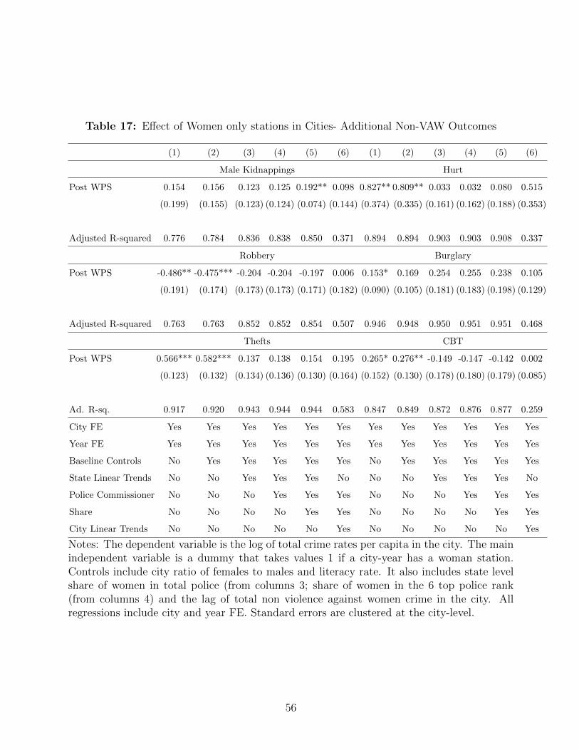
Table 17: Effect of Women only stations in Cities- Additional Non-VAW Outcomes

(1) (2) (3) (4) (5) (6) (1) (2) (3) (4) (5) (6)

Male Kidnappings Hurt

Post WPS 0.154 0.156 0.123 0.125 0.192** 0.098 0.827** 0.809** 0.033 0.032 0.080 0.515

(0.199) (0.155) (0.123) (0.124) (0.074) (0.144) (0.374) (0.335) (0.161) (0.162) (0.188) (0.353)

Adjusted R-squared 0.776 0.784 0.836 0.838 0.850 0.371 0.894 0.894 0.903 0.903 0.908 0.337

Robbery Burglary

Post WPS -0.486** -0.475*** -0.204 -0.204 -0.197 0.006 0.153* 0.169 0.254 0.255 0.238 0.105

(0.191) (0.174) (0.173) (0.173) (0.171) (0.182) (0.090) (0.105) (0.181) (0.183) (0.198) (0.129)

Adjusted R-squared 0.763 0.763 0.852 0.852 0.854 0.507 0.946 0.948 0.950 0.951 0.951 0.468

Thefts CBT

Post WPS 0.566*** 0.582*** 0.137 0.138 0.154 0.195 0.265* 0.276** -0.149 -0.147 -0.142 0.002

(0.123) (0.132) (0.134) (0.136) (0.130) (0.164) (0.152) (0.130) (0.178) (0.180) (0.179) (0.085)

Ad. R-sq. 0.917 0.920 0.943 0.944 0.944 0.583 0.847 0.849 0.872 0.876 0.877 0.259

City FE Yes Yes Yes Yes Yes Yes Yes Yes Yes Yes Yes Yes

Year FE Yes Yes Yes Yes Yes Yes Yes Yes Yes Yes Yes Yes

Baseline Controls No Yes Yes Yes Yes Yes No Yes Yes Yes Yes Yes

State Linear Trends No No Yes Yes Yes No No No Yes Yes Yes No

Police Commissioner No No No Yes Yes Yes No No No Yes Yes Yes

Share No No No No Yes Yes No No No No Yes Yes

City Linear Trends No No No No No Yes No No No No No Yes

Notes: The dependent variable is the log of total crime rates per capita in the city. The mainindependent variable is a dummy that takes values 1 if a city-year has a woman station.Controls include city ratio of females to males and literacy rate. It also includes state levelshare of women in total police (from columns 3; share of women in the 6 top police rank(from columns 4) and the lag of total non violence against women crime in the city. Allregressions include city and year FE. Standard errors are clustered at the city-level.

56

Table

18:

Bas

elin

eE

stim

atio

n-

All

Coeffi

cien

ts

(1)

(2)

(3)

(4)

(5)

(6)

(1)

(2)

(3)

(4)

(5)

(6)

VA

WN

on

-VA

WP

ost

WP

S0.

528*

**0.

553*

**

0.2

84**

0.2

84**

0.3

08**

0.1

94**

0.5

00***

0.5

16**

*0.0

50

0.0

51

0.0

79

0.2

38

(0.1

50)

(0.1

30)

(0.1

23)

(0.1

24)

(0.1

22)

(0.0

93)

(0.1

49)

(0.1

49)

(0.0

56)

(0.0

56)

(0.0

72)

(0.1

47)

Sex

Rat

io1.

104*

*1.1

23***

1.1

19***

2.9

17

3.6

67

0.7

720.6

61

0.6

58

2.7

94

2.1

56

(0.4

88)

(0.3

90)

(0.3

92)

(2.2

72)

(3.3

09)

(0.4

98)

(0.4

20)

(0.4

22)

(2.2

71)

(2.6

90)

Lit

erac

yR

ate

0.88

40.9

50

0.9

15

0.8

39

0.5

10

0.5

740.9

17

0.8

93

0.8

01

0.2

13

(0.6

40)

(0.7

59)

(0.7

41)

(0.8

09)

(0.8

08)

(0.7

29)

(0.9

33)

(0.9

18)

(1.0

03)

(0.9

57)

Pol

ice

Com

mis

sion

er0.1

09

0.1

26

-0.0

62

0.0

73

0.0

94

-0.0

94

(0.1

60)

(0.1

61)

(0.0

75)

(0.1

39)

(0.1

39)

(0.0

66)

Sh

are

-0.0

57

-0.0

51

-7.5

49

-0.0

80*

(0.0

57)

(0.0

57)

(4786721.3

24)

(0.0

47)

N65

265

2634

634

612

630

652

652

634

634

612

630

Ad

just

edR

-sq.

0.94

10.

944

0.9

57

0.9

57

0.9

57

0.4

88

0.9

52

0.9

530.9

59

0.9

59

0.9

61

0.4

37

Cit

yF

EY

esY

esY

esY

esY

esY

esY

esY

esY

esY

esY

esY

esY

ear

FE

Yes

Yes

Yes

Yes

Yes

Yes

Yes

Yes

Yes

Yes

Yes

Yes

Bas

elin

eC

ontr

ols

No

Yes

Yes

Yes

Yes

Yes

No

Yes

Yes

Yes

Yes

Yes

Sta

teL

inea

rT

ren

ds

No

No

Yes

Yes

Yes

No

No

No

Yes

Yes

Yes

No

Pol

ice

Com

mis

sion

erN

oN

oN

oY

esY

esY

esN

oN

oN

oY

esY

esY

esS

har

eof

Fem

ale

Offi

cers

No

No

No

No

Yes

Yes

No

No

No

No

Yes

Yes

Cit

yL

inea

rT

ren

ds

No

No

No

No

No

Yes

No

No

No

No

No

Yes

Nu

mb

erof

city

id73

7373

73

73

71

73

73

73

73

73

71

57

Table

19:

Lis

tof

Cit

ies

over

Tim

e

Sta

teCity

Sta

teCities

Years

Sta

teCity

Sta

teCities

Years

Sta

teCity

Sta

teCities

Years

Andhra

Pra

desh

Hydera

bad

32005-2

013

Kera

laErn

akulu

mCity

42005-2

013

Tamil

Nadu

Coim

bato

re6

2005-2

013

Andhra

Pra

desh

Vijayawada

32005-2

013

Kera

laKochi

42005-2

013

Tamil

Nadu

Madura

i6

2005-2

013

Andhra

Pra

desh

Visakhapatn

am

32005-2

013

Kera

laKozhikode

42005-2

013

Tamil

Nadu

Salem

62005-2

013

Andhra

Pra

desh

Guntu

r7

2010-2

013

Kera

laThiruvananth

apura

m4

2005-2

013

Tamil

Nadu

Thirunelveli

62005-2

013

Andhra

Pra

desh

Rajahmundry

72010-2

013

Kera

laKannur

72012-2

013

Tamil

Nadu

Trichy

62005-2

013

Andhra

Pra

desh

Tirupath

i7

2010-2

013

Kera

laKollam

City

72012-2

013

UttarPra

desh

Agra

11

2005-2

013

Andhra

Pra

desh

Wara

ngal

72010-2

013

Kera

laM

alappura

m7

2012-2

013

UttarPra

desh

Aligarh

11

2005-2

013

Assam

Guwahati

12005-2

011

Kera

laThrissurCity

82013

UttarPra

desh

Allahabad

11

2005-2

013

Assam

Guwahati

22012-2

013

Madhya

Pra

desh

Ash

ok

Nagar

42005-2

013

UttarPra

desh

AmbedakerNagar

11

2005-2

013

Assam

Hamre

n2

2012-2

013

Madhya

Pra

desh

Bhopal

42005-2

013

UttarPra

desh

Bare

illy

11

2005-2

013

Bih

ar

Bagaha

32005-2

013

Madhya

Pra

desh

Indore

42005-2

013

UttarPra

desh

Gora

khpur

11

2005-2

013

Bih

ar

Bettiah

32005-2

013

Madhya

Pra

desh

Jabalp

ur

42005-2

013

UttarPra

desh

Kanpur

11

2005-2

013

Bih

ar

Patn

a3

2005-2

013

Madhya

Pra

desh

Gwalior

62009-2

013

UttarPra

desh

Lucknow

11

2005-2

013

Chandigarh

Chandigarh

12011-2

013

Madhya

Pra

desh

Ujjain

62009-2

013

UttarPra

desh

Meeru

t11

2005-2

013

Chattisgarh

Durg

22005-2

013

Mahara

shtra

Amra

vati

10

2005-2

013

UttarPra

desh

Mora

dabad

11

2005-2

013

Chattisgarh

Raip

ur

22005-2

013

Mahara

shtra

Aura

ngabad

10

2005-2

013

UttarPra

desh

Vara

nasi

11

2005-2

013

Gujara

tAhmedabad

62005-2

013

Mahara

shtra

Mumbai

10

2005-2

013

UttarPra

desh

Pra

vuddh

Nagar

12

2011-2

013

Gujara

tBhavnagar

62005-2

013

Mahara

shtra

MumbaiCommr.

10

2005-2

013

UttarPra

desh

Bhim

Nagar

15

2011-2

013

Gujara

tHim

atn

agar

62005-2

013

Mahara

shtra

Nagpur

10

2005-2

013

UttarPra

desh

CSM

Nagar

15

2011-2

013

Gujara

tRajkot

62005-2

013

Mahara

shtra

Nasik

10

2005-2

013

West

Bengal

Asa

nso

l3

2005-2

013

Gujara

tSura

t6

2005-2

013

Mahara

shtra

NaviM

umbai

10

2005-2

013

West

Bengal

Howra

hCity

32005-2

013

Gujara

tVadodara

62005-2

013

Mahara

shtra

Pune

10

2005-2

013

West

Bengal

Kolkata

32005-2

013

Gujara

tJamnagar

72013

Mahara

shtra

Solapur

10

2005-2

013

Rajasthan

Ajm

er

72005-2

013

Hary

ana

Faridabad

12005-2

013

Mahara

shtra

Thane

10

2005-2

013

Rajasthan

Bhara

tpur

72005-2

013

Hary

ana

Ambala

Urb

an

22012-2

013

Punjab

Amritsar

52005-2

013

Rajasthan

Bikaner

72005-2

013

Jhark

hand

Dhanbad

22005-2

013

Punjab

Jagra

on

52005-2

013

Rajasthan

Jaip

ur

72005-2

013

Jhark

hand

Jamsh

edpur

22005-2

013

Punjab

Jalandhar

52005-2

013

Rajasthan

Jodhpur

72005-2

013

Jhark

hand

Dhanbad

32011-2

013

Punjab

Ludhiana

52005-2

013

Rajasthan

Kota

72005-2

013

Karn

ata

ka

Bangalore

72005-2

013

Punjab

Majith

a5

2005-2

013

Rajasthan

Udaip

ur

72005-2

013

Karn

ata

ka

Belgaum

72005-2

013

Karn

ata

ka

KolarGold

Field

s7

2005-2

013

Karn

ata

ka

Dharw

ad

City

72005-2

013

Karn

ata

ka

Myso

re7

2005-2

013

Karn

ata

ka

Gulb

arg

a7

2005-2

013

Karn

ata

ka

Mangalore

82012-2

013

Karn

ata

ka

Hubli

Dharw

ad

72005-2

013

Tamil

Nadu

Chennai

62005-2

013

Not

es:

Lis

tof

citi

esby

stat

ew

ith

info

rmar

tion

on

the

years

the

data

isav

ailable

for

each

city

.T

he

tab

leals

osh

ows

the

tota

lnu

mb

erof

citi

esp

erst

ate.

58

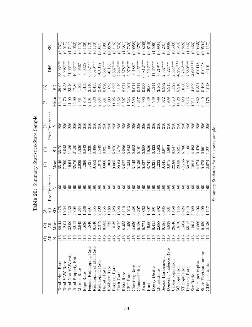
Table

20:

Sum

mar

ySta

tist

ics-

Sta

teSam

ple

(1)

(2)

(3)

(1)

(2)

(3)

(1)

(2)

(3)

All

All

All

Pre

-Tre

atm

ent

Post

-Tre

atm

ent

Diff

SE

NM

ean

SD

NM

ean

SD

NM

ean

SD

Tot

alcr

ime

Rat

e41

689

.44

42.7

5160

65.4

635.7

0256

104.4

39.9

238.9

6***

(3.7

67)

Tot

alV

AW

Rat

e41

612

.04

10.2

4160

7.7

90

8.0

43

256

14.7

010.5

86.9

08***

(0.9

17)

Tot

alN

on-V

AW

rate

416

32.9

022

.30

160

19.9

411.8

6256

41.0

023.4

621.0

6***

(1.7

41)

Tot

alP

rop

erty

Rat

e41

642

.12

20.0

8160

35.7

621.8

0256

46.0

917.8

610.3

3***

(2.0

52)

Mu

rder

Rat

e41

62.

949

1.284

160

2.9

29

1.5

26

256

2.9

61

1.1

09

0.0

567

(0.1

15)

Rap

eR

ate

416

1.63

61.

286

160

1.2

96

0.8

43

256

1.8

48

1.4

59

0.0

325

(0.1

39)

Fem

ale

Kid

nap

pin

gR

ate

416

1.84

01.

897

160

1.4

21

1.3

30

256

2.1

01

2.1

40

0.5

52***

(0.1

13)

Kid

nap

pin

gof

Men

Rat

e41

60.

540

0.455

160

0.5

52

0.4

88

256

0.5

33

0.4

33

0.6

79***

(0.1

70)

Kid

nap

pin

gR

ate

416

2.37

92.

203

160

1.9

72

1.5

49

256

2.6

34

2.4

96

-0.0

197

(0.0

471)

Dac

oity

Rat

e41

60.

583

0.75

5160

0.6

66

0.9

21

256

0.5

31

0.6

26

0.6

61***

(0.1

98)

Rob

ber

yR

ate

416

1.73

21.

180

160

1.3

03

1.1

86

256

2.0

00

1.0

95

-0.1

35

(0.0

826)

Bu

rgla

ryR

ate

416

10.3

95.

623

160

9.0

05

5.9

70

256

11.2

55.2

23

0.6

97***

(0.1

16)

Th

eft

Rat

e41

623

.72

13.2

0160

20.8

414.7

8256

25.5

211.7

92.2

44***

(0.5

74)

Rio

tsR

ate

416

8.45

58.

110

160

6.6

27

6.0

96

256

9.5

97

8.9

71

4.6

78***

(1.3

81)

CB

TR

ate

416

1.45

01.

013

160

1.3

34

0.8

43

256

1.5

23

1.1

01

2.9

70***

(0.7

39)

Ch

eati

ng

Rat

e41

64.

650

4.428

160

3.1

45

2.6

83

256

5.5

90

5.0

11

0.1

88*

(0.0

958)

Cou

nte

rfei

tin

g41

60.

186

0.207

160

0.1

36

0.1

91

256

0.2

17

0.2

11

2.4

46***

(0.3

78)

Ars

on41

60.

774

0.86

2160

0.4

27

0.5

88

256

0.9

90

0.9

33

0.0

812***

(0.0

200)

Hu

rt41

619

.60

19.0

7160

8.7

41

10.5

6256

26.3

920.0

60.5

63***

(0.0

746)

Dow

ryD

eath

s41

60.

455

1.091

160

0.3

21

0.4

22

256

0.5

39

1.3

44

17.6

5***

(1.5

06)

Mol

esta

tion

s41

62.

688

2.892

160

1.2

32

1.5

02

256

3.5

99

3.1

69

0.2

19**

(0.0

904)

Sex

ual

Har

assm

ent

416

0.58

50.

985

160

0.4

45

0.9

77

256

0.6

72

0.9

82

2.3

67***

(0.2

31)

Dom

esti

cV

iole

nce

Rat

e41

64.

838

5.68

1160

3.0

75

4.8

04

256

5.9

39

5.9

13

0.2

27**

(0.0

986)

Urb

anp

opu

lati

on41

626

.46

10.6

8160

22.8

88.5

47

256

28.7

011.2

72.8

64***

(0.5

30)

SC

pop

ula

tion

416

16.7

06.

145

160

20.5

85.5

21

256

14.2

85.2

10

-6.2

96***

(0.5

44)

ST

pop

ula

tion

416

1.56

49.

424

160

-0.7

65

6.7

86

256

3.0

20

10.5

03.7

85***

(0.8

48)

Lit

erac

yR

ate

416

55.1

212

.19

160

50.2

611.0

0256

58.1

511.9

27.8

89***

(1.1

45)

Sex

Rat

io41

610

6.5

5.02

9160

108.8

4.4

93

256

105.1

4.8

29

-3.6

88***

(0.4

66)

Pol

ice

per

cap

ita

416

4.86

60.

403

160

4.8

74

0.4

76

256

4.8

62

0.3

51

-0.0

118

(0.0

435)

Sta

teE

lect

ion

du

mm

y41

60.

459

0.499

160

0.4

75

0.5

01

256

0.4

49

0.4

98

-0.0

258

(0.0

504)

GD

Pp

erca

pit

a41

62.

136

1.11

7160

2.0

74

1.2

21

256

2.1

75

1.0

48

0.1

01

(0.1

17)

Su

mm

ary

Sta

tist

ics

for

the

state

ssa

mp

le.

59

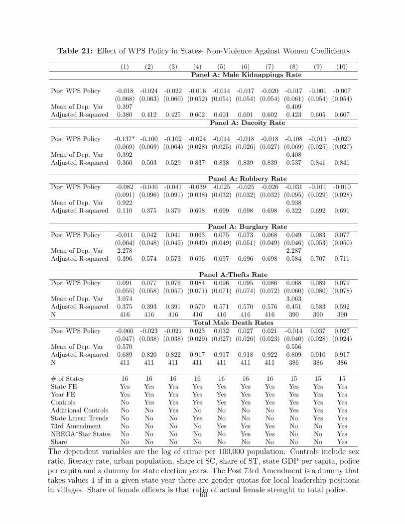
Table 21: Effect of WPS Policy in States- Non-Violence Against Women Coefficients

(1) (2) (3) (4) (5) (6) (7) (8) (9) (10)Panel A: Male Kidnappings Rate

Post WPS Policy -0.018 -0.024 -0.022 -0.016 -0.014 -0.017 -0.020 -0.017 -0.001 -0.007(0.068) (0.063) (0.060) (0.052) (0.054) (0.054) (0.054) (0.061) (0.054) (0.054)

Mean of Dep. Var 0.397 0.409Adjusted R-squared 0.380 0.412 0.425 0.602 0.601 0.601 0.602 0.423 0.605 0.607

Panel A: Dacoity Rate

Post WPS Policy -0.137* -0.100 -0.102 -0.024 -0.014 -0.018 -0.018 -0.108 -0.015 -0.020(0.069) (0.069) (0.064) (0.028) (0.025) (0.026) (0.027) (0.069) (0.025) (0.027)

Mean of Dep. Var 0.392 0.408Adjusted R-squared 0.360 0.503 0.529 0.837 0.838 0.839 0.839 0.537 0.841 0.841

Panel A: Robbery RatePost WPS Policy -0.082 -0.040 -0.041 -0.039 -0.025 -0.025 -0.026 -0.031 -0.011 -0.010

(0.091) (0.096) (0.091) (0.038) (0.032) (0.032) (0.032) (0.095) (0.029) (0.028)Mean of Dep. Var 0.922 0.938Adjusted R-squared 0.110 0.375 0.379 0.698 0.699 0.698 0.698 0.322 0.692 0.691

Panel A: Burglary RatePost WPS Policy -0.011 0.042 0.041 0.063 0.075 0.073 0.068 0.049 0.083 0.077

(0.064) (0.048) (0.045) (0.049) (0.049) (0.051) (0.049) (0.046) (0.053) (0.050)Mean of Dep. Var 2.278 2.287Adjusted R-squared 0.396 0.574 0.573 0.696 0.697 0.696 0.698 0.584 0.707 0.711

Panel A:Thefts RatePost WPS Policy 0.091 0.077 0.076 0.084 0.096 0.095 0.086 0.068 0.089 0.079

(0.055) (0.058) (0.057) (0.071) (0.071) (0.074) (0.072) (0.060) (0.080) (0.078)Mean of Dep. Var 3.074 3.063Adjusted R-squared 0.375 0.393 0.391 0.570 0.571 0.570 0.576 0.451 0.583 0.592N 416 416 416 416 416 416 416 390 390 390

Total Male Death RatesPost WPS Policy -0.060 -0.023 -0.021 0.023 0.032 0.027 0.021 -0.014 0.037 0.027

(0.047) (0.038) (0.038) (0.029) (0.027) (0.026) (0.023) (0.040) (0.028) (0.024)Mean of Dep. Var 0.570 0.556Adjusted R-squared 0.689 0.820 0.822 0.917 0.917 0.918 0.922 0.809 0.910 0.917N 411 411 411 411 411 411 411 386 386 386

# of States 16 16 16 16 16 16 16 15 15 15State FE Yes Yes Yes Yes Yes Yes Yes Yes Yes YesYear FE Yes Yes Yes Yes Yes Yes Yes Yes Yes YesControls No Yes Yes Yes Yes Yes Yes Yes Yes YesAdditional Controls No No Yes No No No No Yes Yes YesState Linear Trends No No No Yes No No No No Yes Yes73rd Amendment No No No No Yes Yes Yes No No YesNREGA*Star States No No No No No Yes Yes No No YesShare No No No No No No No No No Yes

The dependent variables are the log of crime per 100,000 population. Controls include sexratio, literacy rate, urban population, share of SC, share of ST, state GDP per capita, policeper capita and a dummy for state election years. The Post 73rd Amendment is a dummy thattakes values 1 if in a given state-year there are gender quotas for local leadership positionsin villages. Share of female officers is that ratio of actual female strenght to total police.

60

Table

22:

Eff

ect

ofW

PS

Pol

icy

inSta

tes-

Dis

pla

yof

all

coeffi

cien

ts

VA

WF

-Kid

.M

-Kid

.R

ap

eD

aco

ity

Rob

ber

yB

urg

lary

Th

efts

F-D

eath

sM

urd

erL

ove

M-

Dea

ths

Pos

tW

PS

Pol

icy

0.20

1**

0.096

*-0

.020

-0.0

40

-0.0

18

-0.0

26

0.0

68

0.0

86

0.0

10

-0.0

01*

0.0

21

(0.0

72)

(0.0

51)

(0.0

54)

(0.0

28)

(0.0

27)

(0.0

32)

(0.0

49)

(0.0

72)

(0.0

13)

(0.0

01)

(0.0

23)

Pos

rQ

uot

a0.

243*

*0.

112*

*0.0

02

0.0

40

0.0

36

0.0

45

0.0

31

0.0

26

0.0

23

-0.0

00

0.0

21

(0.0

93)

(0.0

47)

(0.0

30)

(0.0

34)

(0.0

26)

(0.0

51)

(0.0

55)

(0.0

52)

(0.0

14)

(0.0

00)

(0.0

19)

NR

EG

A*S

tar

-0.1

970.

139

0.052

-0.0

74

0.1

00**

-0.0

14

0.0

16

-0.0

03

0.0

30

0.0

01

0.0

95

(0.1

65)

(0.1

05)

(0.0

75)

(0.0

99)

(0.0

45)

(0.1

17)

(0.1

60)

(0.1

28)

(0.0

29)

(0.0

01)

(0.0

55)

Sh

are

-0.0

05-0

.002

-0.0

08

-0.0

05

0.0

00

-0.0

02

-0.0

13

-0.0

21*

-0.0

05

0.0

00

-0.0

14***

(0.0

11)

(0.0

05)

(0.0

05)

(0.0

08)

(0.0

04)

(0.0

08)

(0.0

08)

(0.0

11)

(0.0

03)

(0.0

00)

(0.0

05)

Inco

me

p.c

.-0

.108

-0.2

31**

-0.0

51

0.0

90

-0.0

99**

0.0

92

-0.0

94

-0.2

36**

-0.0

47

-0.0

02*

-0.1

03*

(0.1

43)

(0.0

86)

(0.0

59)

(0.0

68)

(0.0

37)

(0.1

12)

(0.0

97)

(0.1

03)

(0.0

38)

(0.0

01)

(0.0

54)

Sex

Rat

io0.

061

-0.0

16-0

.149**

0.0

11

-0.0

43

-0.0

27

0.0

28

-0.0

04

-0.0

15

-0.0

01

-0.0

51

(0.1

13)

(0.0

74)

(0.0

69)

(0.0

46)

(0.0

33)

(0.0

64)

(0.0

62)

(0.0

93)

(0.0

20)

(0.0

01)

(0.0

35)

Urb

anp

op.

-0.0

17-0

.011

0.028***

0.0

10

0.0

22**

0.0

19

0.0

06

0.0

38*

-0.0

07

-0.0

00

-0.0

24**

(0.0

23)

(0.0

07)

(0.0

09)

(0.0

06)

(0.0

09)

(0.0

24)

(0.0

08)

(0.0

21)

(0.0

05)

(0.0

00)

(0.0

11)

SC

-0.0

010.

037

0.070

-0.0

03

0.0

16

0.1

52**

0.0

55

0.0

60

0.0

21

0.0

01

0.0

58

(0.1

07)

(0.0

70)

(0.0

51)

(0.0

42)

(0.0

32)

(0.0

68)

(0.0

74)

(0.0

99)

(0.0

23)

(0.0

01)

(0.0

40)

ST

0.00

4*0.

004*

-0.0

02

0.0

02

-0.0

01

-0.0

03*

-0.0

01

-0.0

01

-0.0

00

0.0

00

-0.0

01***

(0.0

02)

(0.0

02)

(0.0

02)

(0.0

02)

(0.0

01)

(0.0

02)

(0.0

02)

(0.0

03)

(0.0

00)

(0.0

00)

(0.0

00)

Lit

erac

yR

ate

0.01

80.

043*

0.017

-0.0

12

0.0

02

-0.0

11

0.0

30

0.0

37

0.0

01

0.0

00*

0.0

07

(0.0

22)

(0.0

21)

(0.0

15)

(0.0

11)

(0.0

09)

(0.0

23)

(0.0

29)

(0.0

25)

(0.0

04)

(0.0

00)

(0.0

09)

Pol

ice

p.c

.0.

158*

0.09

3*-0

.098

-0.0

07

-0.0

04

-0.1

29**

-0.0

33

-0.0

30

0.0

17

0.0

00

-0.0

00

(0.0

84)

(0.0

50)

(0.0

58)

(0.0

43)

(0.0

31)

(0.0

54)

(0.0

73)

(0.0

90)

(0.0

15)

(0.0

01)

(0.0

21)

Ele

ctio

nY

ear

-0.0

70*

-0.0

03-0

.004

-0.0

07

-0.0

01

0.0

05

0.0

03

-0.0

02

0.0

02

-0.0

00

0.0

13

(0.0

40)

(0.0

16)

(0.0

12)

(0.0

14)

(0.0

13)

(0.0

19)

(0.0

14)

(0.0

21)

(0.0

05)

(0.0

00)

(0.0

09)

N41

641

6416

416

416

416

416

416

411

400

411

#of

Sta

tes

1616

16

16

16

16

16

16

16

16

16

Ad

j.R

-sq.

0.96

0.88

0.6

00.8

40.8

40.7

00.7

00.5

80.6

70.5

90.9

2S

tate

FE

Yes

Yes

Yes

Yes

Yes

Yes

Yes

Yes

Yes

Yes

Yes

Yea

rF

EY

esY

esY

esY

esY

esY

esY

esY

esY

esY

esY

esC

ontr

ols

Yes

Yes

Yes

Yes

Yes

Yes

Yes

Yes

Yes

Yes

Yes

Ad

dit

ion

alC

ontr

ols

Yes

Yes

Yes

Yes

Yes

Yes

Yes

Yes

Yes

Yes

Yes

Sta

teL

inea

rT

ren

ds

Yes

Yes

Yes

Yes

Yes

Yes

Yes

Yes

Yes

Yes

Yes

73rd

Am

end

men

tY

esY

esY

esY

esY

esY

esY

esY

esY

esY

esY

esN

RE

GA

*Sta

rS

tate

sY

esY

esY

esY

esY

esY

esY

esY

esY

esY

esY

esS

har

eY

esY

esY

esY

esY

esY

esY

esY

esY

esY

esY

es

61

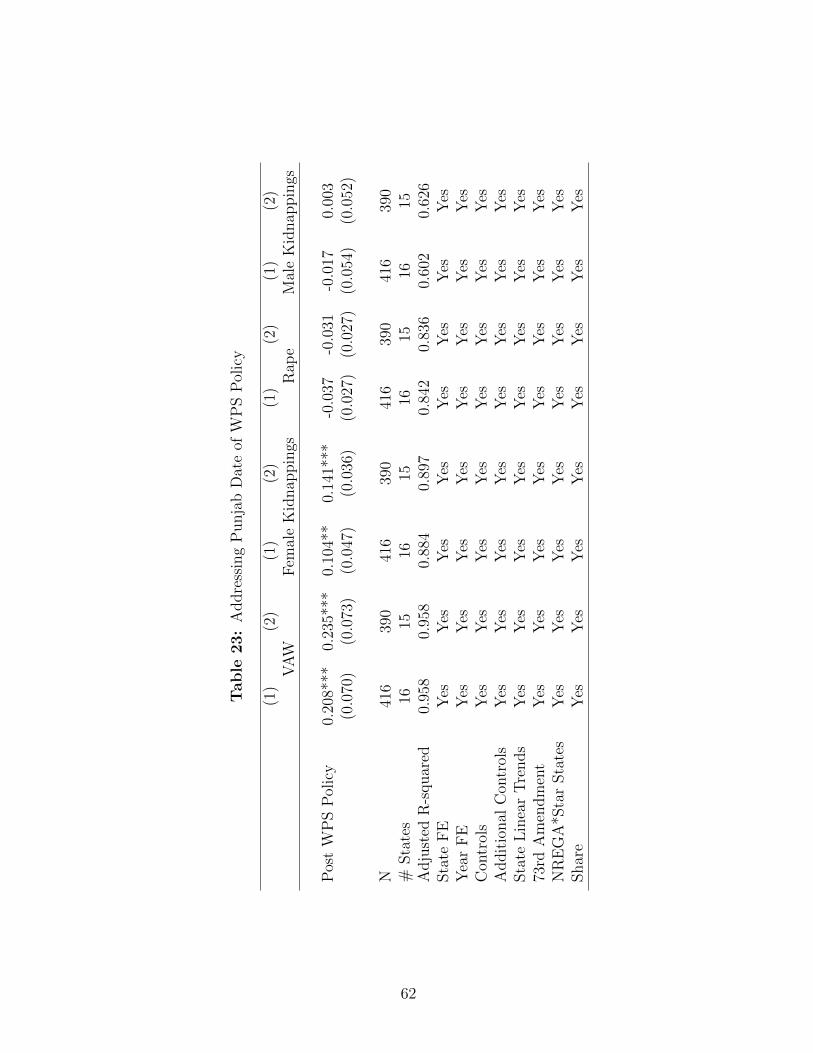
Table

23:

Addre

ssin

gP

unja

bD

ate

ofW

PS

Pol

icy

(1)

(2)

(1)

(2)

(1)

(2)

(1)

(2)

VA

WF

emal

eK

idnap

pin

gsR

ape

Mal

eK

idnap

pin

gs

Pos

tW

PS

Pol

icy

0.20

8***

0.23

5***

0.10

4**

0.14

1***

-0.0

37-0

.031

-0.0

170.

003

(0.0

70)

(0.0

73)

(0.0

47)

(0.0

36)

(0.0

27)

(0.0

27)

(0.0

54)

(0.0

52)

N41

639

041

639

041

639

041

639

0#

Sta

tes

1615

1615

1615

1615

Adju

sted

R-s

quar

ed0.

958

0.95

80.

884

0.89

70.

842

0.83

60.

602

0.62

6Sta

teF

EY

esY

esY

esY

esY

esY

esY

esY

esY

ear

FE

Yes

Yes

Yes

Yes

Yes

Yes

Yes

Yes

Con

trol

sY

esY

esY

esY

esY

esY

esY

esY

esA

ddit

ional

Con

trol

sY

esY

esY

esY

esY

esY

esY

esY

esSta

teL

inea

rT

rends

Yes

Yes

Yes

Yes

Yes

Yes

Yes

Yes

73rd

Am

endm

ent

Yes

Yes

Yes

Yes

Yes

Yes

Yes

Yes

NR

EG

A*S

tar

Sta

tes

Yes

Yes

Yes

Yes

Yes

Yes

Yes

Yes

Shar

eY

esY

esY

esY

esY

esY

esY

esY

es

62

Figure 7: Coefficient Estimates by Iterative Removal of States

Notes: Coefficient estimates of the effects of the roll-out of the WPS in states. The baseline estimatecorresponds to the estimate in Column 7 of Table 6. Each regression estimates the effect of the roll-outof WPS and controls for state and year dummies, sex ratio, literacy rate, share of SC and ST population,income per capita, share of female officers, a dummy for the post 73rd Amendment and a dummy for thepost NREGA roll-out in Star States. The labels indicate that the estimate contains all 16 states except thestate labelled; e.g. estimate AP contains uses the sample of all 15 states except Andhra Pradesh. The labelsrefer to AP Andra Pradesh; ASS Assam; BH Bihar; GJ Gujarat; HR Haryana; HP Himachal Pradesh; KRNKarnataka; KR Kerala; MP Madhya Pradesh; MH Maharashtra; OR Orissa; PJ Punjab; RJ Rajasthan; TNTamil Nadu; UP Uttar Pradesh and WB West Bengal.

63

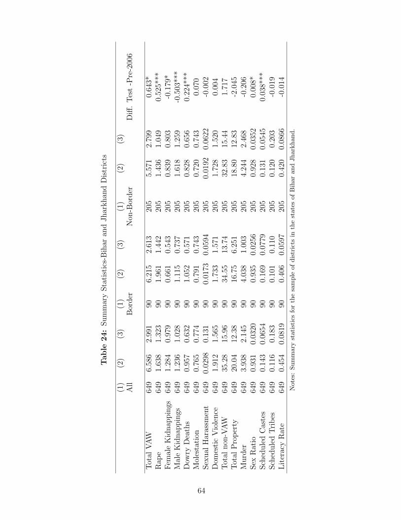
Table

24:

Sum

mar

ySta

tist

ics-

Bih

aran

dJhar

khan

dD

istr

icts

(1)

(2)

(3)

(1)

(2)

(3)

(1)

(2)

(3)

All

Bor

der

Non

-Bor

der

Diff

.T

est

-Pre

-200

6

Tot

alV

AW

649

6.58

62.

991

906.

215

2.61

320

55.

571

2.79

90.

643*

Rap

e64

91.

638

1.32

390

1.96

11.

442

205

1.43

61.

049

0.52

5***

Fem

ale

Kid

nap

pin

gs64

91.

284

0.97

990

0.66

10.

543

205

0.83

90.

803

-0.1

79*

Mal

eK

idnap

pin

gs64

91.

236

1.02

890

1.11

50.

737

205

1.61

81.

259

-0.5

03**

*D

owry

Dea

ths

649

0.95

70.

632

901.

052

0.57

120

50.

828

0.65

60.

224*

**M

oles

tati

on64

90.

765

0.77

490

0.79

10.

743

205

0.72

00.

743

0.07

0Sex

ual

Har

assm

ent

649

0.02

980.

131

900.

0173

0.05

9420

50.

0192

0.06

22-0

.002

Dom

esti

cV

iole

nce

649

1.91

21.

565

901.

733

1.57

120

51.

728

1.52

00.

004

Tot

alnon

-VA

W64

935

.28

15.9

690

34.5

513

.74

205

32.8

315

.44

1.71

7T

otal

Pro

per

ty64

920

.04

12.3

890

16.7

56.

251

205

18.8

012

.83

-2.0

45M

urd

er64

93.

938

2.14

590

4.03

81.

003

205

4.24

42.

468

-0.2

06Sex

Rat

io64

90.

931

0.03

2090

0.93

50.

0256

205

0.92

80.

0352

0.00

8*Sch

edule

dC

aste

s64

90.

143

0.06

5490

0.16

90.

0779

205

0.13

10.

0545

0.03

8***

Sch

edule

dT

rib

es64

90.

116

0.18

390

0.10

10.

110

205

0.12

00.

203

-0.0

19L

iter

acy

Rat

e64

90.

454

0.08

1990

0.40

60.

0597

205

0.42

00.

0866

-0.0

14

Not

es:

Su

mm

ary

stati

stic

sfo

rth

esa

mp

leof

dis

tric

tsin

the

state

sof

Bih

ar

and

Jh

ark

han

d.

64

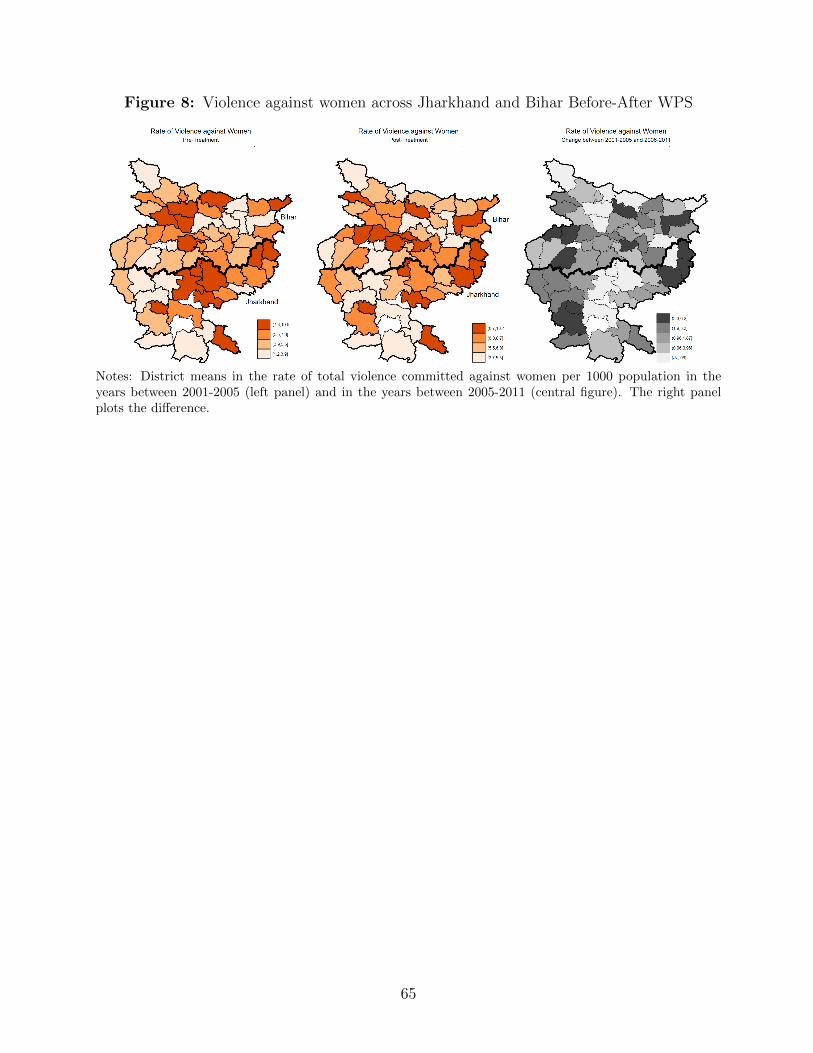
Figure 8: Violence against women across Jharkhand and Bihar Before-After WPS

Notes: District means in the rate of total violence committed against women per 1000 population in theyears between 2001-2005 (left panel) and in the years between 2005-2011 (central figure). The right panelplots the difference.

65

Table 25: Women in the Police and Women-only Stations by State

State Year Women Entered the Police Year WPS Implemented Share of WomenTamil Nadu 1973 1992 5.871Maharashtra 1939 0 4.244Himachal Pradesh 1966 2014 3.150Karnataka 1960 1994 3.020Kerala 1939 1973 3.015Orissa 1961 1994 2.982Rajasthan 1955 1989 2.326Gujarat 1948 1991 2.168Madhya Pradesh 1961 1987 2.111Haryana 1966 2015 2.016Punjab 1949 2010 1.981Uttar Pradesh 1967 1993 1.620Andhra Pradesh 1959 2002 1.520West Bengal 1949 2012 1.469Bihar 1952 2006 1.227Assam 1967 1993 0.491

Notes: This tables presents by state the year in which women were first employed in the law and order;the year in which WPS were implemented and the average sharee of women in the police over the period1988-2013. Note the geographic boundaries of the states are with respect to pre 2001 boundaries. Tablesorted by average share of female officers in states (column 3).

66

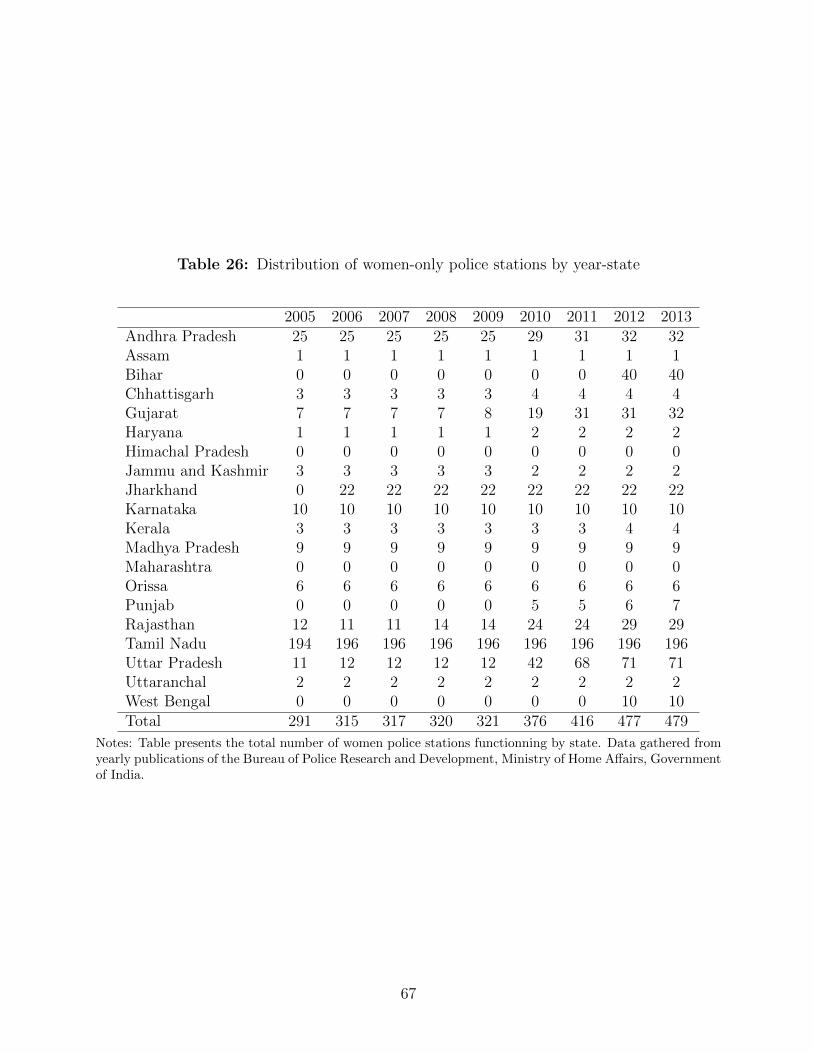
Table 26: Distribution of women-only police stations by year-state

2005 2006 2007 2008 2009 2010 2011 2012 2013Andhra Pradesh 25 25 25 25 25 29 31 32 32Assam 1 1 1 1 1 1 1 1 1Bihar 0 0 0 0 0 0 0 40 40Chhattisgarh 3 3 3 3 3 4 4 4 4Gujarat 7 7 7 7 8 19 31 31 32Haryana 1 1 1 1 1 2 2 2 2Himachal Pradesh 0 0 0 0 0 0 0 0 0Jammu and Kashmir 3 3 3 3 3 2 2 2 2Jharkhand 0 22 22 22 22 22 22 22 22Karnataka 10 10 10 10 10 10 10 10 10Kerala 3 3 3 3 3 3 3 4 4Madhya Pradesh 9 9 9 9 9 9 9 9 9Maharashtra 0 0 0 0 0 0 0 0 0Orissa 6 6 6 6 6 6 6 6 6Punjab 0 0 0 0 0 5 5 6 7Rajasthan 12 11 11 14 14 24 24 29 29Tamil Nadu 194 196 196 196 196 196 196 196 196Uttar Pradesh 11 12 12 12 12 42 68 71 71Uttaranchal 2 2 2 2 2 2 2 2 2West Bengal 0 0 0 0 0 0 0 10 10Total 291 315 317 320 321 376 416 477 479

Notes: Table presents the total number of women police stations functionning by state. Data gathered fromyearly publications of the Bureau of Police Research and Development, Ministry of Home Affairs, Governmentof India.

67

Table

27:

Sum

mar

ySta

tist

ics-

Cit

ySam

ple

NM

ean

SD

NM

ean

SD

NM

ean

SD

All

Tre

atm

ent

Cit

ies

Non

-Tre

atm

ent

Cit

ies

Diff

inM

ean

sC

rim

eR

ates

:T

otal

700

3,9

93

34,3

08

554

4,6

10

38,4

78

146

1,6

50

4,5

49

3,6

70**

Vio

len

ceag

ain

stw

omen

700

534.2

4,6

90

554

625.6

5,2

65

146

187.5

403.1

529.1

**

Dow

ryD

eath

s700

13.8

7111.1

554

15.5

9123.4

146

7.3

44

37.3

99.7

34

Mol

esta

tion

s700

57.9

1460.0

554

64.1

7515.7

146

34.1

471.5

843.3

5*

Sex

ual

Har

assm

ent

700

73.3

3944.1

554

89.9

31,0

61

146

10.3

427.6

490.7

2*

Dom

esti

cV

iole

nce

700

330.5

2,9

62

554

391.6

3,3

25

146

98.5

9230.6

349.3

**

Kid

nap

pin

gof

wom

enan

dG

irls

700

34.6

3213.0

554

38.2

6237.7

146

20.8

554.5

321.9

4*

Pro

per

ty700

2,1

87

18,2

75

554

2,4

83

20,4

63

146

1,0

64

3,3

88

1,8

75*

Tot

alN

on-V

AW

700

2,1

37

18,7

98

554

2,4

94

21,0

95

146

781.7

1,9

97

2,0

56**

Mu

rder

699

51.2

9415.0

553

57.1

2465.0

146

29.2

272.8

734.9

4R

ape

700

24.0

5174.7

554

26.1

1195.6

146

16.2

335.0

514.0

5K

idn

app

ing

700

55.3

1384.8

554

63.1

9431.0

146

25.3

964.9

442.8

1**

Kid

nap

pin

gof

Men

700

20.6

7178.3

554

24.9

3200.1

146

4.5

39

14.2

920.8

7**

Dac

oity

699

5.2

85

34.6

9553

4.5

23

36.0

7146

8.1

71

28.8

0-2

.019

Rob

ber

y700

40.4

2242.9

554

39.0

3265.2

146

45.6

7127.0

5.7

69

Bu

rgla

ry700

374.9

3,1

26

554

409.7

3,4

90

146

242.7

798.5

261.9

Th

eft

700

1,2

66

10,5

43

554

1,4

27

11,7

96

146

655.9

2,1

63

1,0

43*

Rio

ts700

66.9

2432.7

554

61.9

3471.8

146

85.8

8230.1

-12.6

2C

rim

inal

Bre

ach

ofT

rust

700

47.7

9341.9

554

55.0

6383.3

146

20.1

949.9

341.5

2**

Ch

eati

ng

700

451.3

4,0

55

554

545.7

4,5

53

146

93.0

5265.0

521.4

**

Cou

nte

rfei

tin

g699

6.4

74

53.4

0553

6.4

99

59.0

0146

6.3

79

21.8

41.9

83

Ars

on700

13.8

2112.1

554

15.4

5125.4

146

7.6

24

22.3

710.0

2*

Hu

rt700

1,0

59

9,9

73

554

1,2

75

11,2

00

146

238.3

464.1

1,1

72**

Con

trol

s:P

opu

lati

onp

erca

pit

a(l

ogof

)692

13.5

81.3

84

546

13.5

91.1

89

146

13.5

51.9

51

0.1

35

Sex

Rat

io692

0.9

20

0.0

93

546

0.9

20

0.0

970

146

0.9

18

0.0

76

0.0

19***

Lit

erac

yR

ate

689

0.7

26

0.1

21

543

0.7

16

0.1

27

146

0.7

65

0.0

84

-0.0

19**

Pol

ice

Com

mis

sion

er749

0.3

86

0.4

87

575

0.3

39

0.4

74

174

0.5

40

0.5

00

-0.0

795**

Fem

ale

Offi

cers

(%)

727

4.9

14

3.4

73

553

4.4

47

3.2

77

174

6.3

98

3.6

68

-0.6

92**

Sta

tep

olic

est

atio

ns

per

cap

ita

527

0.0

08

0.0

14

410

0.0

07

0.0

103

117

0.0

13

0.0

23

-0.0

04**

Fem

ale

Offi

cers

inT

opp

olic

era

nks

(%)

749

0.0

42

0.0

15

575

0.0

42

0.0

146

174

0.0

42

0.0

15

0.0

03**

Fem

ale

Hea

dC

onst

able

s(%

)749

0.0

21

0.0

05

575

0.0

21

0.0

0499

174

0.0

21

0.0

05

0.0

0F

emal

eC

onst

able

s(%

)749

0.0

49

0.0

12

575

0.0

49

0.0

124

174

0.0

49

0.0

13

0.0

02**

Fem

ale

Insp

ecto

rs(%

)749

0.0

38

0.0

08

575

0.0

38

0.0

0761

174

0.0

38

0.0

08

0.0

01**

Su

mm

ary

Sta

tist

ics

for

the

citi

essa

mp

le.

Cri

me

rate

sare

defi

ned

per

1000

pop

ula

tion

.

68

Table 28: Effect of Women only stations in Cities- Additional Non-VAW Outcomes

(1) (2) (3) (4) (5) (6) (1) (2) (3) (4) (5) (6)

Male Kidnappings Hurt

Post WPS 0.154 0.156 0.123 0.125 0.192** 0.098 0.827** 0.809** 0.033 0.032 0.080 0.515

(0.199) (0.155) (0.123) (0.124) (0.074) (0.144) (0.374) (0.335) (0.161) (0.162) (0.188) (0.353)

Adjusted R-squared 0.776 0.784 0.836 0.838 0.850 0.371 0.894 0.894 0.903 0.903 0.908 0.337

Robbery Burglary

Post WPS -0.486** -0.475*** -0.204 -0.204 -0.197 0.006 0.153* 0.169 0.254 0.255 0.238 0.105

(0.191) (0.174) (0.173) (0.173) (0.171) (0.182) (0.090) (0.105) (0.181) (0.183) (0.198) (0.129)

Adjusted R-squared 0.763 0.763 0.852 0.852 0.854 0.507 0.946 0.948 0.950 0.951 0.951 0.468

Thefts CBT

Post WPS 0.566*** 0.582*** 0.137 0.138 0.154 0.195 0.265* 0.276** -0.149 -0.147 -0.142 0.002

(0.123) (0.132) (0.134) (0.136) (0.130) (0.164) (0.152) (0.130) (0.178) (0.180) (0.179) (0.085)

Ad. R-sq. 0.917 0.920 0.943 0.944 0.944 0.583 0.847 0.849 0.872 0.876 0.877 0.259

City FE Yes Yes Yes Yes Yes Yes Yes Yes Yes Yes Yes Yes

Year FE Yes Yes Yes Yes Yes Yes Yes Yes Yes Yes Yes Yes

Baseline Controls No Yes Yes Yes Yes Yes No Yes Yes Yes Yes Yes

State Linear Trends No No Yes Yes Yes No No No Yes Yes Yes No

Police Commissioner No No No Yes Yes Yes No No No Yes Yes Yes

Share No No No No Yes Yes No No No No Yes Yes

City Linear Trends No No No No No Yes No No No No No Yes

Notes: The dependent variable is the log of total crime rates per capita in the city. The mainindependent variable is a dummy that takes values 1 if a city-year has a woman station.Controls include city ratio of females to males and literacy rate. It also includes state levelshare of women in total police (from columns 3; share of women in the 6 top police rank(from columns 4) and the lag of total non violence against women crime in the city. Allregressions include city and year FE. Standard errors are clustered at the city-level.

69

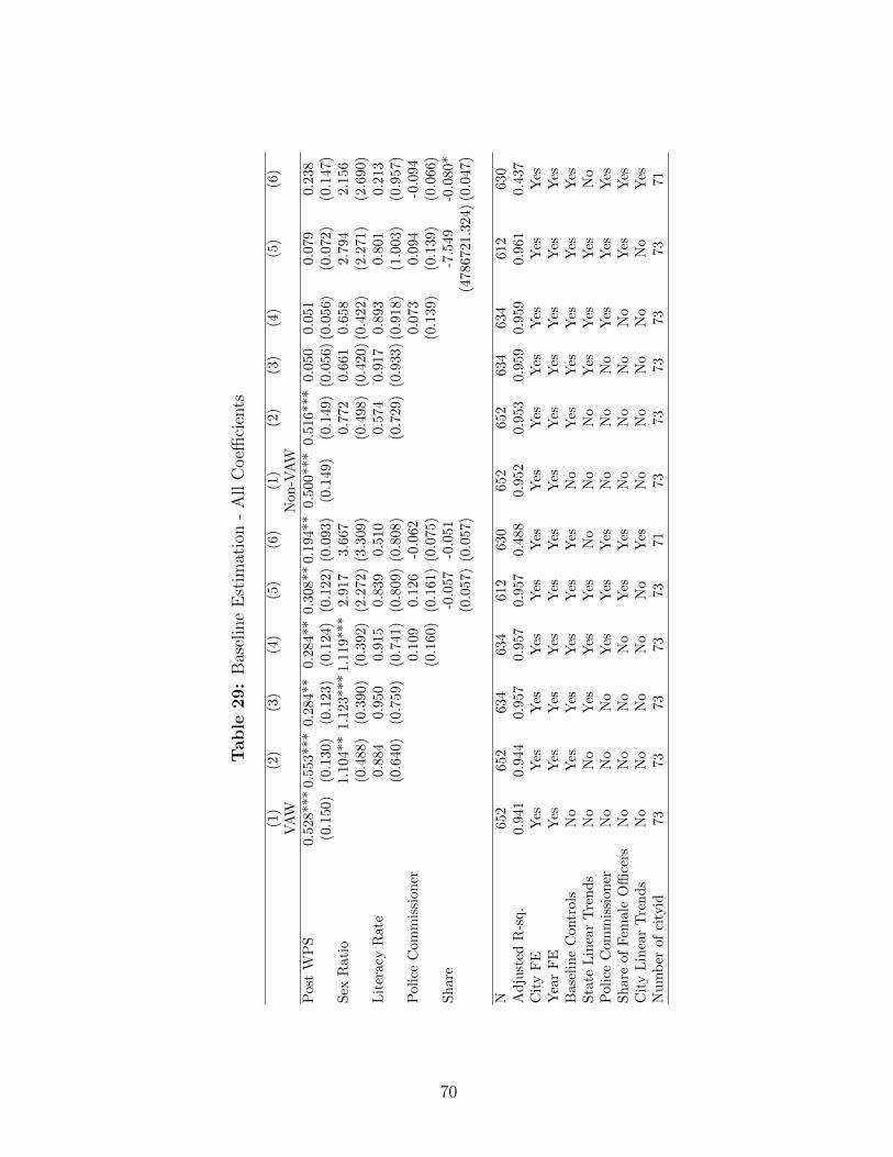
Table

29:

Bas

elin

eE

stim

atio

n-

All

Coeffi

cien

ts

(1)

(2)

(3)

(4)

(5)

(6)

(1)

(2)

(3)

(4)

(5)

(6)

VA

WN

on

-VA

WP

ost

WP

S0.

528*

**0.

553*

**

0.2

84**

0.2

84**

0.3

08**

0.1

94**

0.5

00***

0.5

16**

*0.0

50

0.0

51

0.0

79

0.2

38

(0.1

50)

(0.1

30)

(0.1

23)

(0.1

24)

(0.1

22)

(0.0

93)

(0.1

49)

(0.1

49)

(0.0

56)

(0.0

56)

(0.0

72)

(0.1

47)

Sex

Rat

io1.

104*

*1.1

23***

1.1

19***

2.9

17

3.6

67

0.7

720.6

61

0.6

58

2.7

94

2.1

56

(0.4

88)

(0.3

90)

(0.3

92)

(2.2

72)

(3.3

09)

(0.4

98)

(0.4

20)

(0.4

22)

(2.2

71)

(2.6

90)

Lit

erac

yR

ate

0.88

40.9

50

0.9

15

0.8

39

0.5

10

0.5

740.9

17

0.8

93

0.8

01

0.2

13

(0.6

40)

(0.7

59)

(0.7

41)

(0.8

09)

(0.8

08)

(0.7

29)

(0.9

33)

(0.9

18)

(1.0

03)

(0.9

57)

Pol

ice

Com

mis

sion

er0.1

09

0.1

26

-0.0

62

0.0

73

0.0

94

-0.0

94

(0.1

60)

(0.1

61)

(0.0

75)

(0.1

39)

(0.1

39)

(0.0

66)

Sh

are

-0.0

57

-0.0

51

-7.5

49

-0.0

80*

(0.0

57)

(0.0

57)

(4786721.3

24)

(0.0

47)

N65

265

2634

634

612

630

652

652

634

634

612

630

Ad

just

edR

-sq.

0.94

10.

944

0.9

57

0.9

57

0.9

57

0.4

88

0.9

52

0.9

530.9

59

0.9

59

0.9

61

0.4

37

Cit

yF

EY

esY

esY

esY

esY

esY

esY

esY

esY

esY

esY

esY

esY

ear

FE

Yes

Yes

Yes

Yes

Yes

Yes

Yes

Yes

Yes

Yes

Yes

Yes

Bas

elin

eC

ontr

ols

No

Yes

Yes

Yes

Yes

Yes

No

Yes

Yes

Yes

Yes

Yes

Sta

teL

inea

rT

ren

ds

No

No

Yes

Yes

Yes

No

No

No

Yes

Yes

Yes

No

Pol

ice

Com

mis

sion

erN

oN

oN

oY

esY

esY

esN

oN

oN

oY

esY

esY

esS

har

eof

Fem

ale

Offi

cers

No

No

No

No

Yes

Yes

No

No

No

No

Yes

Yes

Cit

yL

inea

rT

ren

ds

No

No

No

No

No

Yes

No

No

No

No

No

Yes

Nu

mb

erof

city

id73

7373

73

73

71

73

73

73

73

73

71

70

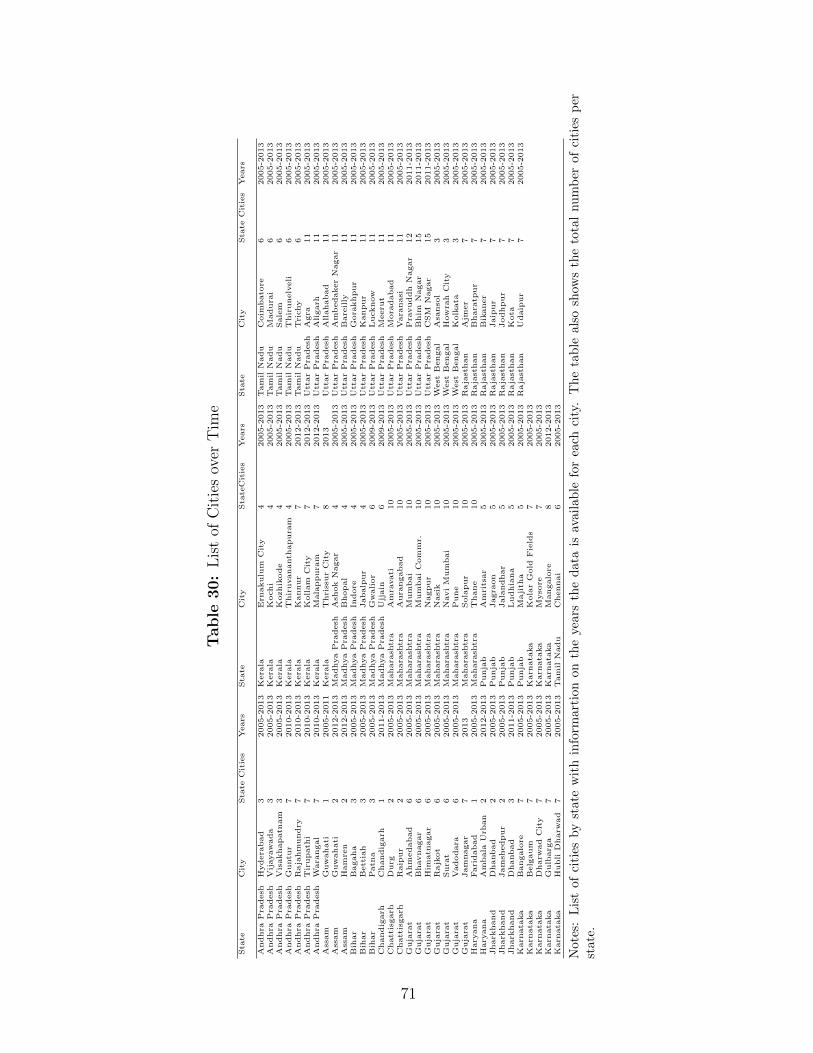
Table

30:

Lis

tof

Cit

ies

over

Tim

e

Sta

teCity

Sta

teCities

Years

Sta

teCity

Sta

teCities

Years

Sta

teCity

Sta

teCities

Years

Andhra

Pra

desh

Hydera

bad

32005-2

013

Kera

laErn

akulu

mCity

42005-2

013

Tamil

Nadu

Coim

bato

re6

2005-2

013

Andhra

Pra

desh

Vijayawada

32005-2

013

Kera

laKochi

42005-2

013

Tamil

Nadu

Madura

i6

2005-2

013

Andhra

Pra

desh

Visakhapatn

am

32005-2

013

Kera

laKozhikode

42005-2

013

Tamil

Nadu

Salem

62005-2

013

Andhra

Pra

desh

Guntu

r7

2010-2

013

Kera

laThiruvananth

apura

m4

2005-2

013

Tamil

Nadu

Thirunelveli

62005-2

013

Andhra

Pra

desh

Rajahmundry

72010-2

013

Kera

laKannur

72012-2

013

Tamil

Nadu

Trichy

62005-2

013

Andhra

Pra

desh

Tirupath

i7

2010-2

013

Kera

laKollam

City

72012-2

013

UttarPra

desh

Agra

11

2005-2

013

Andhra

Pra

desh

Wara

ngal

72010-2

013

Kera

laM

alappura

m7

2012-2

013

UttarPra

desh

Aligarh

11

2005-2

013

Assam

Guwahati

12005-2

011

Kera

laThrissurCity

82013

UttarPra

desh

Allahabad

11

2005-2

013

Assam

Guwahati

22012-2

013

Madhya

Pra

desh

Ash

ok

Nagar

42005-2

013

UttarPra

desh

AmbedakerNagar

11

2005-2

013

Assam

Hamre

n2

2012-2

013

Madhya

Pra

desh

Bhopal

42005-2

013

UttarPra

desh

Bare

illy

11

2005-2

013

Bih

ar

Bagaha

32005-2

013

Madhya

Pra

desh

Indore

42005-2

013

UttarPra

desh

Gora

khpur

11

2005-2

013

Bih

ar

Bettiah

32005-2

013

Madhya

Pra

desh

Jabalp

ur

42005-2

013

UttarPra

desh

Kanpur

11

2005-2

013

Bih

ar

Patn

a3

2005-2

013

Madhya

Pra

desh

Gwalior

62009-2

013

UttarPra

desh

Lucknow

11

2005-2

013

Chandigarh

Chandigarh

12011-2

013

Madhya

Pra

desh

Ujjain

62009-2

013

UttarPra

desh

Meeru

t11

2005-2

013

Chattisgarh

Durg

22005-2

013

Mahara

shtra

Amra

vati

10

2005-2

013

UttarPra

desh

Mora

dabad

11

2005-2

013

Chattisgarh

Raip

ur

22005-2

013

Mahara

shtra

Aura

ngabad

10

2005-2

013

UttarPra

desh

Vara

nasi

11

2005-2

013

Gujara

tAhmedabad

62005-2

013

Mahara

shtra

Mumbai

10

2005-2

013

UttarPra

desh

Pra

vuddh

Nagar

12

2011-2

013

Gujara

tBhavnagar

62005-2

013

Mahara

shtra

MumbaiCommr.

10

2005-2

013

UttarPra

desh

Bhim

Nagar

15

2011-2

013

Gujara

tHim

atn

agar

62005-2

013

Mahara

shtra

Nagpur

10

2005-2

013

UttarPra

desh

CSM

Nagar

15

2011-2

013

Gujara

tRajkot

62005-2

013

Mahara

shtra

Nasik

10

2005-2

013

West

Bengal

Asa

nso

l3

2005-2

013

Gujara

tSura

t6

2005-2

013

Mahara

shtra

NaviM

umbai

10

2005-2

013

West

Bengal

Howra

hCity

32005-2

013

Gujara

tVadodara

62005-2

013

Mahara

shtra

Pune

10

2005-2

013

West

Bengal

Kolkata

32005-2

013

Gujara

tJamnagar

72013

Mahara

shtra

Solapur

10

2005-2

013

Rajasthan

Ajm

er

72005-2

013

Hary

ana

Faridabad

12005-2

013

Mahara

shtra

Thane

10

2005-2

013

Rajasthan

Bhara

tpur

72005-2

013

Hary

ana

Ambala

Urb

an

22012-2

013

Punjab

Amritsar

52005-2

013

Rajasthan

Bikaner

72005-2

013

Jhark

hand

Dhanbad

22005-2

013

Punjab

Jagra

on

52005-2

013

Rajasthan

Jaip

ur

72005-2

013

Jhark

hand

Jamsh

edpur

22005-2

013

Punjab

Jalandhar

52005-2

013

Rajasthan

Jodhpur

72005-2

013

Jhark

hand

Dhanbad

32011-2

013

Punjab

Ludhiana

52005-2

013

Rajasthan

Kota

72005-2

013

Karn

ata

ka

Bangalore

72005-2

013

Punjab

Majith

a5

2005-2

013

Rajasthan

Udaip

ur

72005-2

013

Karn

ata

ka

Belgaum

72005-2

013

Karn

ata

ka

KolarGold

Field

s7

2005-2

013

Karn

ata

ka

Dharw

ad

City

72005-2

013

Karn

ata

ka

Myso

re7

2005-2

013

Karn

ata

ka

Gulb

arg

a7

2005-2

013

Karn

ata

ka

Mangalore

82012-2

013

Karn

ata

ka

Hubli

Dharw

ad

72005-2

013

Tamil

Nadu

Chennai

62005-2

013

Not

es:

Lis

tof

citi

esby

stat

ew

ith

info

rmar

tion

on

the

years

the

data

isav

ailable

for

each

city

.T

he

tab

leals

osh

ows

the

tota

lnu

mb

erof

citi

esp

erst

ate.

71

Table

31:

Sum

mar

ySta

tist

ics-

Sta

teSam

ple

(1)

(2)

(3)

(1)

(2)

(3)

(1)

(2)

(3)

All

All

All

Pre

-Tre

atm

ent

Post

-Tre

atm

ent

Diff

SE

NM

ean

SD

NM

ean

SD

NM

ean

SD

Tot

alcr

ime

Rat

e41

689

.44

42.7

5160

65.4

635.7

0256

104.4

39.9

238.9

6***

(3.7

67)

Tot

alV

AW

Rat

e41

612

.04

10.2

4160

7.7

90

8.0

43

256

14.7

010.5

86.9

08***

(0.9

17)

Tot

alN

on-V

AW

rate

416

32.9

022

.30

160

19.9

411.8

6256

41.0

023.4

621.0

6***

(1.7

41)

Tot

alP

rop

erty

Rat

e41

642

.12

20.0

8160

35.7

621.8

0256

46.0

917.8

610.3

3***

(2.0

52)

Mu

rder

Rat

e41

62.

949

1.284

160

2.9

29

1.5

26

256

2.9

61

1.1

09

0.0

567

(0.1

15)

Rap

eR

ate

416

1.63

61.

286

160

1.2

96

0.8

43

256

1.8

48

1.4

59

0.0

325

(0.1

39)

Fem

ale

Kid

nap

pin

gR

ate

416

1.84

01.

897

160

1.4

21

1.3

30

256

2.1

01

2.1

40

0.5

52***

(0.1

13)

Kid

nap

pin

gof

Men

Rat

e41

60.

540

0.455

160

0.5

52

0.4

88

256

0.5

33

0.4

33

0.6

79***

(0.1

70)

Kid

nap

pin

gR

ate

416

2.37

92.

203

160

1.9

72

1.5

49

256

2.6

34

2.4

96

-0.0

197

(0.0

471)

Dac

oity

Rat

e41

60.

583

0.75

5160

0.6

66

0.9

21

256

0.5

31

0.6

26

0.6

61***

(0.1

98)

Rob

ber

yR

ate

416

1.73

21.

180

160

1.3

03

1.1

86

256

2.0

00

1.0

95

-0.1

35

(0.0

826)

Bu

rgla

ryR

ate

416

10.3

95.

623

160

9.0

05

5.9

70

256

11.2

55.2

23

0.6

97***

(0.1

16)

Th

eft

Rat

e41

623

.72

13.2

0160

20.8

414.7

8256

25.5

211.7

92.2

44***

(0.5

74)

Rio

tsR

ate

416

8.45

58.

110

160

6.6

27

6.0

96

256

9.5

97

8.9

71

4.6

78***

(1.3

81)

CB

TR

ate

416

1.45

01.

013

160

1.3

34

0.8

43

256

1.5

23

1.1

01

2.9

70***

(0.7

39)

Ch

eati

ng

Rat

e41

64.

650

4.428

160

3.1

45

2.6

83

256

5.5

90

5.0

11

0.1

88*

(0.0

958)

Cou

nte

rfei

tin

g41

60.

186

0.207

160

0.1

36

0.1

91

256

0.2

17

0.2

11

2.4

46***

(0.3

78)

Ars

on41

60.

774

0.86

2160

0.4

27

0.5

88

256

0.9

90

0.9

33

0.0

812***

(0.0

200)

Hu

rt41

619

.60

19.0

7160

8.7

41

10.5

6256

26.3

920.0

60.5

63***

(0.0

746)

Dow

ryD

eath

s41

60.

455

1.091

160

0.3

21

0.4

22

256

0.5

39

1.3

44

17.6

5***

(1.5

06)

Mol

esta

tion

s41

62.

688

2.892

160

1.2

32

1.5

02

256

3.5

99

3.1

69

0.2

19**

(0.0

904)

Sex

ual

Har

assm

ent

416

0.58

50.

985

160

0.4

45

0.9

77

256

0.6

72

0.9

82

2.3

67***

(0.2

31)

Dom

esti

cV

iole

nce

Rat

e41

64.

838

5.68

1160

3.0

75

4.8

04

256

5.9

39

5.9

13

0.2

27**

(0.0

986)

Urb

anp

opu

lati

on41

626

.46

10.6

8160

22.8

88.5

47

256

28.7

011.2

72.8

64***

(0.5

30)

SC

pop

ula

tion

416

16.7

06.

145

160

20.5

85.5

21

256

14.2

85.2

10

-6.2

96***

(0.5

44)

ST

pop

ula

tion

416

1.56

49.

424

160

-0.7

65

6.7

86

256

3.0

20

10.5

03.7

85***

(0.8

48)

Lit

erac

yR

ate

416

55.1

212

.19

160

50.2

611.0

0256

58.1

511.9

27.8

89***

(1.1

45)

Sex

Rat

io41

610

6.5

5.02

9160

108.8

4.4

93

256

105.1

4.8

29

-3.6

88***

(0.4

66)

Pol

ice

per

cap

ita

416

4.86

60.

403

160

4.8

74

0.4

76

256

4.8

62

0.3

51

-0.0

118

(0.0

435)

Sta

teE

lect

ion

du

mm

y41

60.

459

0.499

160

0.4

75

0.5

01

256

0.4

49

0.4

98

-0.0

258

(0.0

504)

GD

Pp

erca

pit

a41

62.

136

1.11

7160

2.0

74

1.2

21

256

2.1

75

1.0

48

0.1

01

(0.1

17)

Su

mm

ary

Sta

tist

ics

for

the

state

ssa

mp

le.

72

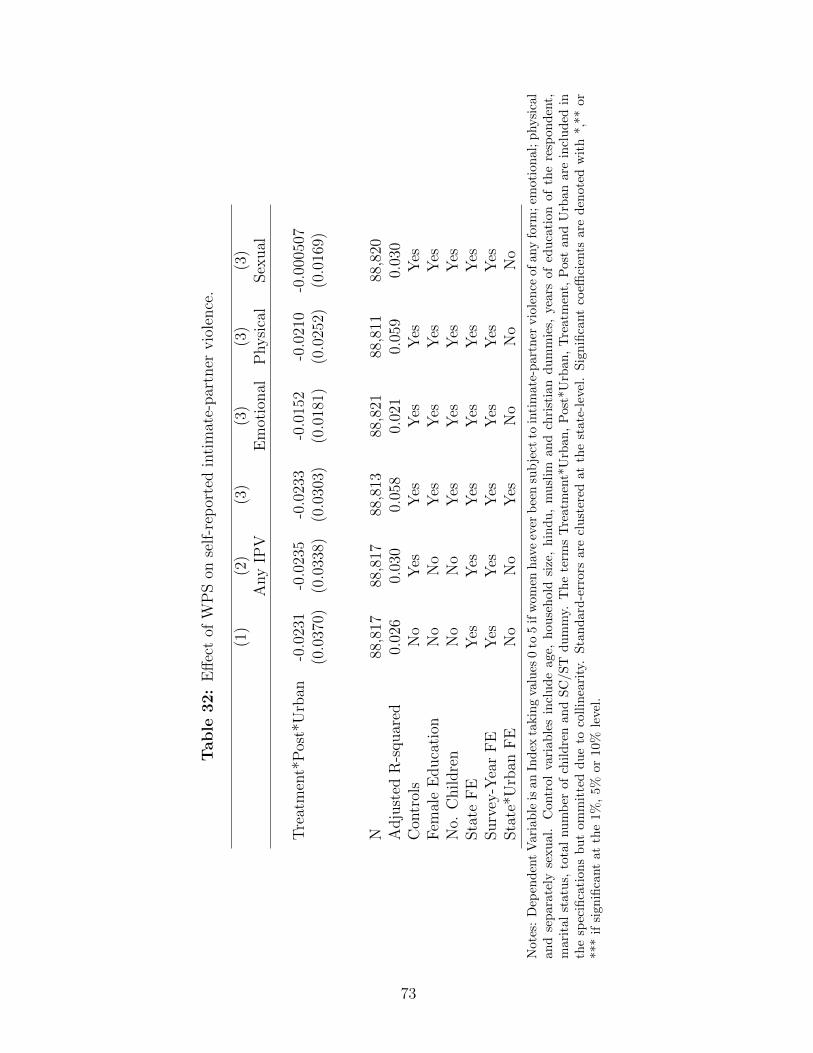
Table

32:

Eff

ect

ofW

PS

onse

lf-r

epor

ted

inti

mat

e-par

tner

vio

lence

.

(1)

(2)

(3)

(3)

(3)

(3)

Any

IPV

Em

otio

nal

Physi

cal

Sex

ual

Tre

atm

ent*

Pos

t*U

rban

-0.0

231

-0.0

235

-0.0

233

-0.0

152

-0.0

210

-0.0

0050

7(0

.037

0)(0

.033

8)(0

.030

3)(0

.018

1)(0

.025

2)(0

.016

9)

N88

,817

88,8

1788

,813

88,8

2188

,811

88,8

20A

dju

sted

R-s

quar

ed0.

026

0.03

00.

058

0.02

10.

059

0.03

0C

ontr

ols

No

Yes

Yes

Yes

Yes

Yes

Fem

ale

Educa

tion

No

No

Yes

Yes

Yes

Yes

No.

Childre

nN

oN

oY

esY

esY

esY

esSta

teF

EY

esY

esY

esY

esY

esY

esSurv

ey-Y

ear

FE

Yes

Yes

Yes

Yes

Yes

Yes

Sta

te*U

rban

FE

No

No

Yes

No

No

No

Not

es:

Dep

end

ent

Var

iab

leis

anIn

dex

takin

gva

lues

0to

5if

wom

enh

ave

ever

bee

nsu

bje

ctto

inti

mate

-part

ner

vio

len

ceofany

form

;em

oti

on

al;

physi

cal

and

separ

atel

yse

xu

al.

Con

trol

vari

able

sin

clu

de

age,

hou

seh

old

size

,h

ind

u,

mu

slim

an

dch

rist

ian

du

mm

ies,

years

of

edu

cati

on

of

the

resp

on

den

t,m

arit

alst

atu

s,to

tal

nu

mb

erof

chil

dre

nan

dS

C/S

Td

um

my.

Th

ete

rms

Tre

atm

ent*

Urb

an

,P

ost

*U

rban

,T

reatm

ent,

Post

an

dU

rban

are

incl

ud

edin

the

spec

ifica

tion

sb

ut

omm

itte

dd

ue

toco

llin

eari

ty.

Sta

nd

ard

-err

ors

are

clu

ster

edat

the

state

-lev

el.

Sig

nifi

cant

coeffi

cien

tsare

den

ote

dw

ith

*,*

*or

***

ifsi

gnifi

cant

atth

e1%

,5%

or10

%le

vel.

73

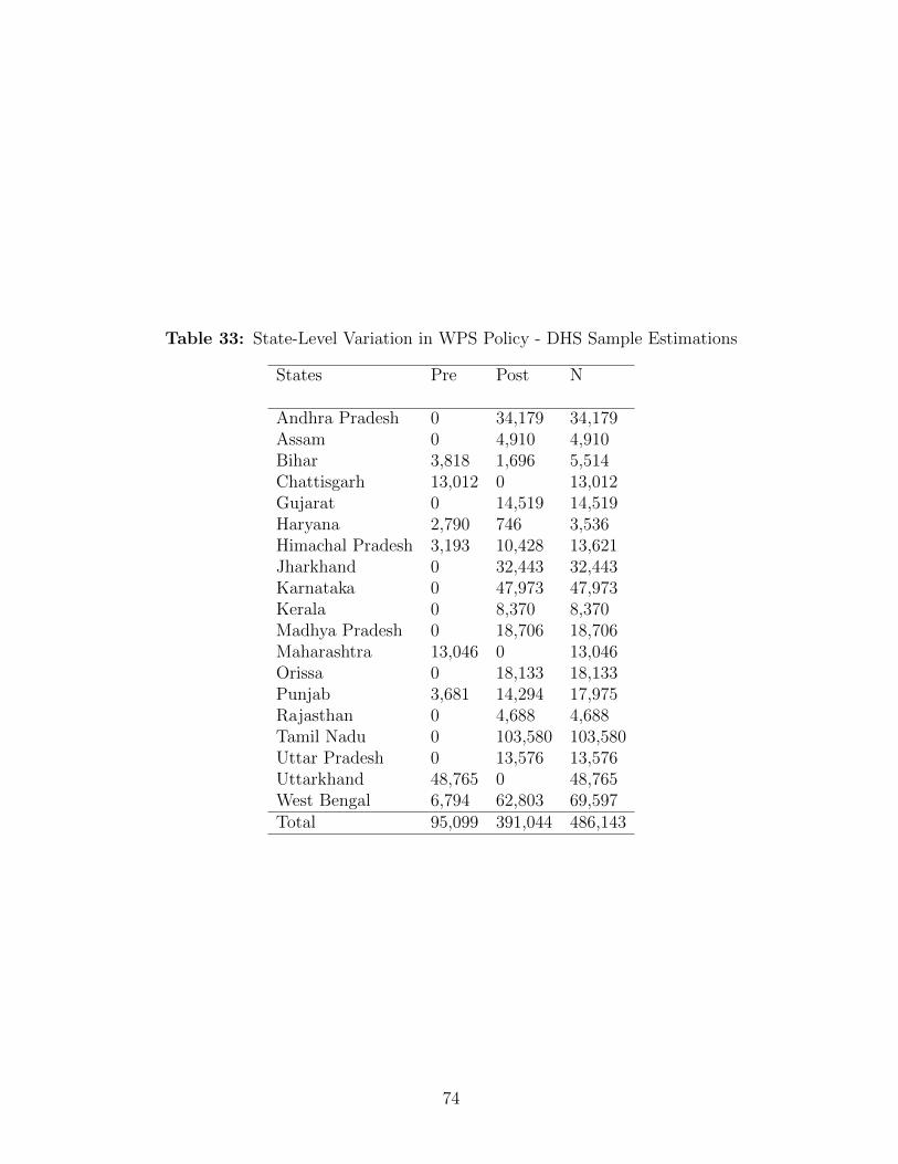
Table 33: State-Level Variation in WPS Policy - DHS Sample Estimations

States Pre Post N

Andhra Pradesh 0 34,179 34,179Assam 0 4,910 4,910Bihar 3,818 1,696 5,514Chattisgarh 13,012 0 13,012Gujarat 0 14,519 14,519Haryana 2,790 746 3,536Himachal Pradesh 3,193 10,428 13,621Jharkhand 0 32,443 32,443Karnataka 0 47,973 47,973Kerala 0 8,370 8,370Madhya Pradesh 0 18,706 18,706Maharashtra 13,046 0 13,046Orissa 0 18,133 18,133Punjab 3,681 14,294 17,975Rajasthan 0 4,688 4,688Tamil Nadu 0 103,580 103,580Uttar Pradesh 0 13,576 13,576Uttarkhand 48,765 0 48,765West Bengal 6,794 62,803 69,597Total 95,099 391,044 486,143

74

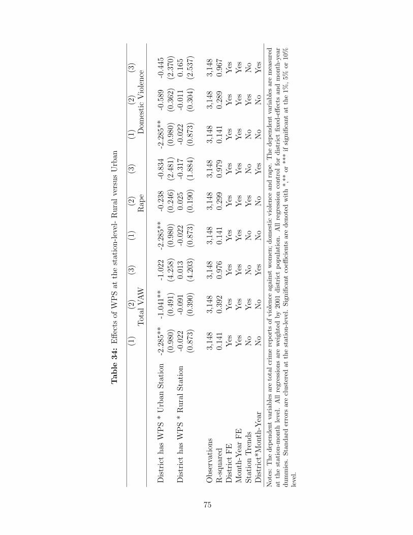
Table

34:

Eff

ects

ofW

PS

atth

est

atio

n-l

evel

-R

ura

lve

rsus

Urb

an

(1)

(2)

(3)

(1)

(2)

(3)

(1)

(2)

(3)

Tot

alV

AW

Rap

eD

omes

tic

Vio

lence

Dis

tric

thas

WP

S*

Urb

anSta

tion

-2.2

85**

-1.0

41**

-1.0

22-2

.285

**-0

.238

-0.8

34-2

.285

**-0

.589

-0.4

45(0

.980

)(0

.491

)(4

.258

)(0

.980

)(0

.246

)(2

.481

)(0

.980

)(0

.362

)(2

.370

)D

istr

ict

has

WP

S*

Rura

lSta

tion

-0.0

22-0

.091

0.01

3-0

.022

0.02

5-0

.317

-0.0

22-0

.011

0.16

5(0

.873

)(0

.390

)(4

.203

)(0

.873

)(0

.190

)(1

.884

)(0

.873

)(0

.304

)(2

.537

)

Obse

rvat

ions

3,14

83,

148

3,14

83,

148

3,14

83,

148

3,14

83,

148

3,14

8R

-squar

ed0.

141

0.39

20.

976

0.14

10.

299

0.97

90.

141

0.28

90.

967

Dis

tric

tF

EY

esY

esY

esY

esY

esY

esY

esY

esY

esM

onth

-Yea

rF

EY

esY

esY

esY

esY

esY

esY

esY

esY

esSta

tion

Tre

nds

No

Yes

No

No

Yes

No

No

Yes

No

Dis

tric

t*M

onth

-Yea

rN

oN

oY

esN

oN

oY

esN

oN

oY

es

Not

es:

Th

ed

epen

den

tva

riab

les

are

tota

lcr

ime

rep

ort

sof

vio

len

ceagain

stw

om

en;

dom

esti

cvio

len

cean

dra

pe.

Th

ed

epen

den

tva

riab

les

are

mea

sure

dat

the

stat

ion

-mon

thle

vel.

All

regr

essi

ons

are

wei

ghte

dby

2001

dis

tric

tp

op

ula

tion.

All

regre

ssio

nco

ntr

ol

for

dis

tric

tfi

xed

-eff

ects

an

dm

onth

-yea

rd

um

mie

s.S

tan

dar

der

rors

are

clu

ster

edat

the

stati

on

-lev

el.

Sig

nifi

cant

coeffi

cien

tsare

den

ote

dw

ith

*,*

*or

***

ifsi

gn

ifica

nt

at

the

1%

,5%

or

10%

leve

l.

75