GEMS data assimilation system for chemically reactive gases

587

GEMS data assimilation system for chemically reactive gases

Antje Inness, Johannes Flemming, Martin Suttie and Luke Jones

Research Department

May 2009

Series: ECMWF Technical Memoranda

A full list of ECMWF Publications can be found on our web site under:http://www.ecmwf.int/publications/

Contact: [email protected]

c©Copyright 2009

European Centre for Medium-Range Weather ForecastsShinfield Park, Reading, RG2 9AX, England

Literary and scientific copyrights belong to ECMWF and are reserved in all countries. This publication is notto be reprinted or translated in whole or in part without the written permission of the Director. Appropriatenon-commercial use will normally be granted under the condition that reference is made to ECMWF.

The information within this publication is given in good faith and considered to be true, but ECMWF acceptsno liability for error, omission and for loss or damage arising from its use.

http://www.ecmwf.int/publications/


Abstract

A data assimilation system for chemically reactive gases has been developed at the European Centre forMedium-Range Weather Forecasts (ECMWF) for the ”Global and regional Earth-system Monitoring usingSatellite and in-situ data” (GEMS) project. ECMWF’s integrated forecast system (IFS) was extended toinclude the chemically reactive gases ozone, carbon monoxide, nitrogen oxides, formaldehyde and sulphurdioxide. Chemical transport models were coupled to the IFS using the OASIS4 coupler to model the chem-ical processes and to provide the IFS with chemical production and loss rates. This paper describes theassimilation system for the reactive gases, presents the background error statistics developed for the reactivegases, and shows some first results of the assimilation of satellite retrievals for all five new species.

1 Introduction

The EU-funded GEMS (Global and regional Earth-system Monitoring using Satellite and in-situ data) projectis developing a comprehensive data analysis and modelling system for monitoring the global distribution of at-mospheric constituents important for climate, air quality and UV radiation, with a focus on Europe. As part ofthe project a pre-operational data assimilation and forecasting system for aerosols, greenhouse gases and chem-ically reactive gases has been developed by extending ECMWF’s Integrated Forecast System (IFS), allowingECMWF’s 4D-VAR data assimilation system to be used to assimilate satellite observations of atmosphericcomposition at global scale (Hollingsworth et al. 2008).

This paper focuses on the assimilation system for chemically reactive gases developed under the global reactivegases (GRG) subproject of GEMS. Information about the aerosol subproject can be found in Benedetti et al.(2009) and about the greenhouse gases subproject in Engelen et al. (2009). The GRG subproject focuses onthe assimilation of the following gases: Ozone (O3), carbon monoxide (CO), nitrogen oxides (NOx = NO +NO2), formaldehyde (HCHO) and sulphur dioxide (SO2). These gases play a key role in the chemistry of theatmosphere and are observable from space.

Ozone is crucially important for the chemistry of the troposphere. Tropospheric ozone is a regional scalepollutant and at high concentrations near the surface, it is harmful to humans and vegetation (National ResearchCouncil 1991). Photolysis of ozone, followed by reaction with water vapour, provides the primary source ofthe hydroxyl radical (OH), the main atmospheric oxidant, in the troposphere (e.g. Logan et al. 1981). Ozoneis also a significant greenhouse gas, particularly in the upper troposphere (Hansen et al. 1997). The majorityof tropospheric ozone formation occurs when NOx, CO, and volatile organic compounds (VOCs) react in theatmosphere in the presence of sunlight. These ozone precursors are emitted by traffic and industrial activities.In urban areas in the Northern Hemisphere (NH), high ozone levels usually occur during the summer.

CO is one of the most important trace gases in the troposphere and affects the concentrations of the OH radical.CO has natural and anthropogenic sources (see reviews by Seinfeld and Randis (2006) and Kanakidou andCrutzen (1999)). It is emitted from the soil, plants and the ocean, but the main sources of CO are incompletefossil fuel and biomass burning, which lead to enhanced surface concentrations. The highest CO concentrationsare found over the industrial regions of Europe, Asia and North America. Surface concentrations are higherduring the winter than during the summer months because of the shorter lifetime in the summer due to higherOH concentrations and more intense mixing processes. Tropical biomass burning is most intense during thedry season (December-April in the NH tropics, July-October in SH tropics). CO has a lifetime of a few monthsand can serve as a tracer for regional and inter-continental transport of polluted air.

NOx plays a key role in tropospheric chemistry and is the main ingredient in the formation of ground levelozone. Its sources are anthropogenic emission (traffic, industry, power plants), biomass burning (Crutzen andSchmailzl 1983), soil emissions (Granli and Bokman 1994) and lightning (Martin et al. 2007). NOx has a

Technical Memorandum No. 587 1


lifetime of a few days or less in the boundary layer, so that concentrations are larger over land than over thecleaner oceans. The largest concentrations are found over industrial and urban regions of the Eastern US,California, Europe, China and Japan.

HCHO is one of the most abundant hydrocarbons in the atmosphere. It is formed in most Non-Methane hy-drocarbon (NMHC) oxidation chains. Its primary emission sources are industrial activities, and fossil fuel andbiomass burning. The largest contribution to the HCHO budget is its large secondary source from the oxida-tion of VOCs (Atkinson 1994), the main precursors being methane and isoprene. The main sinks of HCHOare photolysis and oxidation by OH. HCHO has a short lifetime of a few hours, making it a good indicator ofhydrocarbon emission areas.

SO2 contributes to acid rain and is a key precursor for sulphuric acid aerosol formation. At high concentrations,it can affect human health, in particular in combination with fog (smog). Anthropogenic activities such as fossilfuel burning and metal smelting have raised atmospheric SO2 concentrations by up to 3 orders of magnitudeover the last century (Pham et al. 1996). Another source for SO2 are volcanic eruptions that can eject largeamounts of SO2 into the atmosphere. The ash and SO2 emitted by volcanic eruptions are a major hazard toaviation. In the troposphere SO2 has a lifetime of a few days, in the stratosphere several weeks.

For the assimilation of tropospheric reactive gases it is important to have a complex chemistry scheme in themodel and assimilation system, so that chemical source and sink processes can be accounted for. For theGEMS system it was deemed premature and numerically too expensive to include a complex chemistry schemein the IFS. Instead, chemical transport models (CTMs) coupled to the IFS are used to provide the chemicaltendencies for the IFS. The OASIS4 coupler (Valcke and Redler 2006) is used to couple the three CTMsMOZART (Kinnison et al. 2007; Horowitz et al. 2003), MOCAGE (Josse et al. 2004) and TM5 (Krol et al.2005) to the IFS. Any one of these CTMs can then be used to provide chemical production and loss rates forthe GRG fields to the IFS. The CTM in turn is driven by meteorological fields from the IFS. The reactive gasesincluded in the IFS can then be restrained by the assimilation of satellite data from various instruments.

This paper describes the GEMS reactive gases data assimilation system and shows some first results from theassimilation of O3, CO, NOx, HCHO, and SO2 satellite data with the coupled GEMS system.

2 Coupled IFS GRG system

The GEMS data assimilation system for chemically reactive gases was constructed by extending ECMWF’sintegrated forecast system (IFS) to include fields for O3, CO, NOx, HCHO, and SO2. Chemical productionand loss rates (chemical tendencies) for these gases are supplied by a CTM that is coupled to the IFS using theOASIS4 coupler. Technically, it is possible to couple any one of the three CTMs MOZART, MOCAGE andTM5 to the IFS. The IFS supplies the meteorological data to the CTM every hour, and the CTM provides IFSwith initial conditions for the tracers and with three dimensional tendency fields every hour.

The reactive gas O3 had already been included in the IFS as an additional model variable, and ozone data havebeen assimilated at ECMWF since 1999 (Holm et al. 1999, Dethof and Holm 2004). However, the ECMWFapproach differes from the GEMS approach because it uses an inbuilt chemistry routine with a parametrizationof photochemical sources and sinces based on an updated version of Cariolle and Deque (1999) instead if acoupled CTM to provied the chemical tendencies.

All the experiments described in this paper use a setup where the MOZART CTM is coupled to the IFS witha coupling frequency of 1 hour. This CTM was chosen because it is the numerically least expensive one ofthe three CTMs, and it is not feasible to run long assimilation experiments with a numerically more expensiveCTM. A description of the MOZART CTM as implemented in the GEMS system can be found in Stein (2009).

2 Technical Memorandum No. 587


2.1 Data assimilation

2.1.1 4D-Var

ECMWF has used an incremental formulation of 4-dimensional variational data assimilation (4D-Var) since1997. In 4D-Var a cost function is minimized to combine the model background and the observations to obtainthe best possible forecast by adjusting the initial conditions. In its incremental formulation (Courtier et al.1994) 4D-Var can be written as

J(δx) =12

δxT B−1δx+12(Hδx−d)T R−1(Hδx−d), (1)

where δx is the increment, B the background error covariance matrix, R the observation error covariance matrix(comprising of observational and representativeness errors), and H a linear approximation of the observationoperator. d = y−Hxb is the innovation vector, y the observation vector and xb the background.

The GRG fields are fully integrated into the ECMWF variational analysis as additional model variables. Theyare minimized together with the main ECMWF fields, which means they can, in priciple, influence the analysisof wind and other meteorological variables in 4D-Var. However, given the uncertainty of the GRG observationsand the lack of observational constraints of variables such as wind or temperature in the stratosphere andmesosphere, a possible influence of the GRG observations on the meteorological fields is currently suppressed.

2.1.2 Background errors for the reactive gases

In the ECMWF data assimilation system the background error covariance matrix is given in a wavelet for-mulation (Fisher 2004, 2006). This allows both spatial and spectral variations of the horizontal and verticalbackground error covariances. The background error correlations used for the ECMWF variables were derivedfrom an ensemble of forecast difference, using a method proposed by Fisher and Andersson (2001).

The standard deviations determine the relative weight of the background in the analysis, the correlations deter-mine how the analysis increments are spread in the horizontal and in the vertical. This is particularly importantfor vertically integrated observations, such as total column observation. In this case the vertical structure of theincrements is entirely determined by the vertical correlations of the background errors since the observationsdo not give information about this distribution.

The GRG background errors are univariate in order to minimize the feedback effects of the GRG fields on theother variables. For the GEMS ozone field the IFS ozone background error statistics obtained by the ensem-ble method are used. These are the same background error statistics that are used in ECMWF’s operationalozone assimilation. Figure 1 shows vertical profiles of the standard deviation, and the horizontal and verticalcorrelations of the ozone background errors at 50◦N, 10◦E.

A different method had to be chosen to determine background error statistics for the other GRG fields becausethey had not been included in the ensemble of forecast runs. The NMC method (Parrish and Derber 1992) wasused to derive initial background error statistics for the reactive gases. For this, 150 days of 2-day forecastswere run with the coupled system initialized from fields produced by the free running MOZART CTM, and thedifferences between 24-h and 48-h forecasts valid at the same time were used as a proxy for the backgrounderrors. These differences were then used to construct a wavelet background error covariance matrix accordingto the method described by Fisher (2004, 2006). This background error covariance matrix contains the statisticsfor the reactive gases as well as the original statistics for the other meteorological fields.



0 5e−08 1e−07 1.5e−07 2e−07

0

20

40

60

mod

el le

vel

100 20 30 40 50 60model level

60

50

40

30

20

10

mod

el le

vel

0.1 0.2

0.5

0.9

0 200 400 600 800 1000distance (km)

60

50

40

30

20

10

mod

el le

vel

0.020.05

0.10.20.

5

Figure 1: Ozone background error standard deviation profile (top left) in kg/kg, vertical correlations of ozone background errors (topright), and horizontal correlations of ozone background errors (bottom) at 50◦N,10◦E.

The background error statistics for CO were determined with the NMC method. Figure2 shows vertical pro-files of the standard deviation of the CO background errors and the horizontal and vertical correlations of thebackground errors for CO at 50◦N, 10◦E. The standard deviation values in model levels 1 to 19 were set to thevalue of level 20 to prevent large increments near the model top.

The background errors for HCHO calculated with the NMC method had long horizontal correlations that led tounrealistic increments far away from observations, for example over the polar regions. Therefore the statisticsobtained with the NMC method were modified, and a globally constant standard deviation profile was used forHCHO. This was taken from the NMC statistics at 0◦ latitude, 0◦ longitude. The background error standarddeviations were multiplied by a factor 10, because the values obtained with the NMC method were too small anddid not give reasonable HCHO increments in single observation experiments. A diagonal vertical correlationmatrix was used, and a prescribed structure function with a length scale of 150 km was used for the horizonalcorrelations. The HCHO background error standard deviation profile is shown in Figure3 (left plot).



0

20

40

60

mod

el le

vel

100 20 30 40 50 60model level

60

50

40

30

20

10

mod

el le

vel

0.05

0.02

0.1

0.2

0.5

0 200 400 600 800 1000distance (km)

60

50

40

30

20

10

mod

el le

vel

0 1e−08 2e−08 3e−08 4e−08

0.9

0.5 0.50.2

0.1

Figure 2: CO background error standard deviation profile (top left) in kg/kg, vertical correlations of CO background errors at (topright), and horizontal correlations of CO background errors (bottom) at 50◦N, 10◦E.

For the assimilation of NOx data it was found that the analysis based on mixing ratio was prone to largeextrapolation errors, due to the high variability of NOx in space and time and the difficulties in modeling theerror covariances. Therefore a logarithmic control variable was developed for NOx. The NMC statistics forNOx were calculated from the differences of the natural logarithm of the 24h and 48h forecast fields. Like inthe case of HCHO, long horizontal correlations led to unrealistic increments far away from observations, and aglobally constant standard deviation profile was used (NMC statistics at 0◦ latitude, 0◦ longitude) together witha diagonal vertical correlation matrix, and a prescribed structure function with a length scale of 150 km for thehorizonal correlations. The standard deviation profile of the LOG NOx statistics are shown in Figure3 (rightplot).

SO2 observations are only assimilated in the GEMS system in the event of large volcanic eruptions, i.e. whenthe observed SO2 concentrations are considerably larger than the atmospheric background values. An NMCapproach would not give useful background error statistics for SO2 for these cases as the forecast model doesnot have information about individual volcanic eruptions, even though it includes a subaerial volcano emissions



0.00e+00 5.00e−10 1.00e−09 1.50e−09 2.00e−09

0

20

40

60

mod

el le

vel

0 0.5 1 1.5

0

20

40

60

mod

el le

vel

Figure 3: Vertical profiles of the background error standard deviation for HCHO (left) in kg/kg and and NOx (right), dimensionless.

climatology. Therefore, background error statistics for SO2 were constructed by prescribing a background errorstandard deviation profile that peaks at model level 36 and 37, corresponding to an SO2 injection height of about6 km (see Figure 4). A diagonal vertical correlation matrix, and a prescribed structure function with length scaleof 150 km for the horizonal correlations are used SO2 as for NOx and HCHO.

0 5e−07 1e−06 1.5e−06 2e−06

0

20

40

60

mod

el le

vel

Figure 4: Profile of background error standard deviation for volcanic SO2 in kg/kg for an injection height of 6 km (left).

2.1.3 Observation errors for reactive gases

The observation error and background error covariance matrices determine the relative weight given to theobservation and the background in the analysis. For the reactive gases observation errors given by the dataproviders are used. If this value is below 5%, a minimum value of 5% is taken. The observation error isassumed to include a representativeness error that arises because of differences in resolution of observation andthe model, and that accounts for scales unresolved by the model.



2.1.4 Observation operators for reactive gases

The observations of chemically reactive gases that are assimilated into the IFS are satellite retrievals. Theseobservations are total or partial column data, i.e. integrated layers bounded by a top and a bottom pressure. Theunit for the reactive gases observations used in IFS is kg/m2. The IFS background fields are interpolated intime and space to the location of the observation, and the model’s first-guess is calculated as a simple verticalintegral between the top and the bottom pressure given by the partial or total column.

It is also possible to use averaging kernels provided by the data producers in the observation operator. In thiscase, the model equivalent of the observation is calculated using the averaging kernel weights and pressures.

NO2 - NOx interconversion The fast diurnal NO2 - NO interconversion caused by solar radiation in the upperstratosphere can not be handled by the coupled system with a coupling frequency of one hour. Therefore NOxis used as the model variable instead of NO2. The NOx field is not so strongly influenced by solar radiationand the chemical development of the NOx field can be simulated better by the coupled system. The use of NOxalso reduces spatial variablity everywhere which is of advantage for the data assimilation. Since the satelliteobservations assimilated in the GEMS system are NO2 data, a diagnostic NO2/NOx interconversion operatorwas developed, including its tangent linear and adjoint. This operator is based on a simple photochemicalequilibrium between NO2 and NO:

[NO2][NOx]

=k[O3]

JNO2+ k[O3]. (2)

Here k is the rate coefficient of the reaction of O3 with NO to NO2 and O3 and depends on temperature, andJNO2 is the NO2 photolysis frequency and depends on surface albedo, solar zenith angle, overhead ozone col-umn, cloud optical properties and temperature. A parameterised approach for the calculation of JNO2 was usedbased on the band scheme by Landgraf and Crutzen (1998) in combination with actinic fluxes parameterisedfollowing Krol and Van Weele (1997). The diagnostic operator includes the effect of clouds, surface albedoand overhead ozone columns. Information for these fields is taken from the IFS. The parameterization wasextended to include an adjustment to the equilibrium because of hydro-carbons in the lower troposphere andabundant O-radical in the higher stratosphere and mesosphere. An ad-hoc approach was introduced to accountfor the influence of per-oxy-radical concentration by assuming a per-oxy-radical (HO2 + RO2) concentrationof 80 ppt (Kleinman et al. 1995) in the troposphere, which was scaled by the cosine of the solar zenith angle toaccount for the diurnal cycle of the per-oxy-radical concentration.

2.1.5 Bias correction and quality control for reactive gases

For the initial analysis experiments with the GEMS coupled system no bias correction is used for the reactivegases. This will be addressed in further studies.

Variational quality control and first-guess checks are applied to the reactive gases observations, apart from SO2

observations.

2.2 Coupling and resolution

In the coupled setup the IFS and the CTM run in parallel, exchanging fields through the OASIS4 coupler everyhour. This means the IFS supplies the meteorological data and updated mixing ratios for the GEMS speciesO3, CO, NOx, HCHO, and SO2 to the CTM every hour, and the CTM provides IFS with initial conditions for



the GEMS species and with chemical tendency fields every hour. These are tendencies due to chemistry, wetdeposition and atmospheric emissions, and tendencies due to surface fluxes (emission, dry deposition). Thetendencies are combined before the exchange and one total tendency is given from the CTM to the IFS.

The data assimilation algorithm for the GRG fields in the coupled system follows the assimilation of the IFSozone with the parameterized chemistry (Holm et al. 1999; Dethof and Holm 2004). The implementationof the incremental solution for the 4D-VAR data assimilation problem is structured into an outer and innerloop. The outer loop, or trajectory run, is an IFS run with the complete model at high horizontal resolution todetermine the increments between the model and the observations. The inner loop, or minimization run, is runwith a linearized model version and its adjoint formulation at a lower resolution. The simplified model usedin the inner loop acts on the increments to solve the minimization problem of the 4D-VAR cost function. Thesequence of outer and inner loop is repeated two or more times to determine the final analysis. The time lengthof the assimilation window is 12 hours, and analyses valid every 6 hours are produced. A forecast run startedfrom the previous analysis provides the starting point for the assimilation in the next 12h window.

The IFS-CTM coupling is applied in the outer loops. The inner loops using the tangent linear and adjoint modelare currently run uncoupled, i.e. without the application of the source and sink tendencies from the CTM. Thesubsequent forecast that provides the starting point for the next analysis cycle is run coupled.

In the coupled system the IFS runs at a T159 spectral resolution and the grid point space is represented ina reduced Gaussian grid (Hortal and Simmons 1991). The vertical coordinate system is given by 60 hybridsigma-pressure levels, with a model top at 0.1 hPa. In order to avoid difficulties in the vertical interpolationby the OASIS4 coupler, the CTMs use the same 60 vertical levels. The coupler only has to perform horizontalinterpolations for which the bi-linear mode is applied. The resolution of the CTMs is between 2◦ and 3◦, lowerthan the IFS resolution, because of the high computational cost of the CTMs. The IFS is run on a higherhorizontal resolution because of the quality of the meteorological forecasts and because a lower resolutionwould limit the acceptance of high resolution observations within data assimilation. The coupling frequency is3600 s which is the largest acceptable time step for the IFS at a T159 resolution. More details of the CTMs andthe coupling setup are given in Flemming et al. (2009).

3 Results

This section presents some results of the assimilation of O3, CO, NOx, HCHO and SO2 obtained with thecoupled GEMS assimilation system. Data for the assimilation of O3 and CO are taken from a GRG reanalysisrun for the period May to December 2003 (GRGAN), in which the MOZART CTM was coupled to the IFSand GRG data were assimilated in addition to the meteorological data assimilated at ECMWF during 2003.These GRG data include MOPITT total column CO data, total column O3 data from SCIAMACHY, and partialO3 columns from MIPAS, GOME and SBUV/2. In addition to GRGAN, a control experiment was run, inwhich the GRG data were only included passively (GRGCTRL). A comprehensive evaluation of GRGAN andGRGCTRL is done elsewhere (e.g. Ordonez et al. 2009; Elguindi et al. 2009; GEMS GRG validation report2009). Here only some examples for O3 and CO are shown.

NO2 and HCHO data were not assimilated in GRGAN, because the technical development for the assimilationof those fields had not been completed. SO2 was not included in the version of the MOZART model that wasused for these coupled runs. The examples for the assimilation of NO2, HCHO and SO2 that are shown hereare taken from other assimilation experiments.



3.1 GEMS O3 assimilation

The ozone retrievals assimilated in GRGAN are total column ozone fields from SCIAMACHY produced byKNMI, GOME ozone profiles produced by the Rutherford Appleton Laboratory, MIPAS ozone profiles pro-duced by ESA, and SBUV/2 partial columns from NOAA. Because MIPAS measures in the mid-infrared partof the spectrum, MIPAS ozone data are the only data used here that are available independent of illuminationcondition, including during the polar night. The SCIAMACHY data are thinned to a horizontal resolution of0.5◦x0.5◦, the other ozone data are not thinned. SCIAMACHY, GOME and SBUV/2 ozone data are not used atlow solar elevations, and GOME and SBUV/2 data are not used poleward of 80◦. Profile data are not assimilatedabove 1 hPa.

Figure 5 shows timeseries of zonal mean total column ozone from GRGAN, GRGCTRL and independentTOMS data for the period 1 May to 31 December 2003. The total column timeseries from GRGAN agrees wellwith the independent TOMS data. It shows high values at high northern latitudes and in SH midlatitudes, lowervalues in the tropics, and the very low values of the Antarctic Ozone hole between September and November.The control experiment agrees less well with the TOMS data. It underestimates total column ozone in theTropics, and overestimates it in SH midlatitudes. The Antarctic ozone hole is not deep enough in GRGCTRL,and zonal mean ozone values are 100 Dobson Units higher in GRGCTRL than in GRGAN at the peak of theozone hole. This overestimation of the ozone column in the SH was also found in standalone runs with theMOZART CTM (GEMS GRG validation report 2009).

Figure 6 depicts seasonal mean plots of total column ozone for June to August (JJA) and September to Novem-ber (SON) 2003 (left panels) from GRGAN, and the difference between GRGAN and GRGCTRL (right panels).It shows that the assimilation leads to reduced ozone columns in the NH extratropics and to increased valuesin the tropics in both seasons in GRGAN. The control run overestimates the stratospheric ozone maximum inthe NH extratropics and underestimates it in the tropics, and the assimilation corrects this. This leads to theimproved agreement with TOMS data seen in Figure 5. In SH midlatitudes and over the South Pole the con-trol run overestimates the ozone columns, and the assimilation leads to reduced total column ozone values inGRGAN.

The largest change in total ozone column between GRGAN and GRGCTRL is seen over the South Pole wherethe ozone hole is not deep enough in GRGCTRL (Figures 5 and 6). Figure 7 takes a closer look at the ozonefield over the South Pole on 4 October 2003. It shows a cross section of ozone across the South pole along 8◦Efrom GRGAN (top), GRGCTRL (middle), as well as ozone profiles from an independent ozone sonde launchedat Neumayer (71◦S, 8◦E) and from GRGAN and GRGCTRL. Both, the cross sections and the ozone profiles,illustrate that the depletion of ozone over the South Pole in the layer between 25-150 hPa is completely missingin the control run, while GRGAN shows low ozone values over the pole and agrees well with the ozone sondeobservation.

The examples shown here illustrate that the assimilation of ozone data in the GEMS coupled system leads to animproved total column ozone field in comparison with the control run. The analysis also improves the verticalstructure of the GEMS ozone field if ozone profile data, such as MIPAS or GOME profiles, are assimilated.Total column and profiles from GRGAN agree well with independent observations from TOMS and ozonesondes.

3.2 CO assimilation

Total column CO retrievals from MOPITT version 003 (Deeter et al. 2003) are assimilated in GRGAN. The dataare thinned to a resolution of 0.5◦x0.5◦ and are only assimilated over land between 65◦N and 65◦S. Averaging



-80

-60

-40

-20

0

20

40

60

80La

titud

e

-80

-60

-40

-20

0

20

40

60

80

Latit

ude

-80

-60

-40

-20

0

20

40

60

80

Latit

ude

100 – 125 125 – 150 150 – 175 175 – 200 200 – 225 225 – 250 250 – 275 275 – 300300 – 325 325 – 350 350 – 375 375 – 400 400 – 425 425 – 450 450 – 475 475 – 600

1 13 25 6 18 30 12 24 5 17 29 10 22 4 16 28 9 21 3 15 27MAY JUN JUL AUG SEP OCT NOV DEC

1 13 25 6 18 30 12 24 5 17 29 10 22 4 16 28 9 21 3 15 27JUN JUL AUG SEP OCT NOV DEC

1 13 25 6 18 30 12 24 5 17 29 10 22 4 16 28 9 21 3 15 27MAY

MAY

JUN JUL AUG SEP OCT NOV DEC

Figure 5: Timeseries of zonal mean total column ozone in Dobson Units for the period 1 May 2003 till 31 December 2003 from TOMSdata (top), GRGAN (middle) and GRGCTRL (bottom).



250

250 250

250

250

250

275275

275

275275275

275275 275

300

300

300

300300300

300

300

300

325

325

325325 325325

325

325

100

150

200

250

300

350

400

-60

-30

0

30

60

175

175

200

200200

225

225 225

250

250 250

250

250

275

275

275

275

275

275

275 275

275

300

300

300

300300300

300

300300300

300

325

325

325

325

325

325

325

350

350

100

150

200

250

300

350

400

-60

-30

0

30

60

Figure 6: Mean total column GEMS ozone field in Dobson Units averaged over the seasons JJA (top) and SON (bottom). The leftpanels show GRGAN, the right panels the difference between GRGAN and GRGCTRL (GRGAN minus GRGCTRL) also in DobsonUnits.

kernel information from the MOPITT data is not used in the experiments presented here.

Figure 8 shows a timeseries of globally averaged CO total column first-guess and analysis departures andtheir standard deviations, as well as the number of observations used per analysis cycle between May andDecember 2003. Plotted are statistics for data that are actively used in the analysis. The timeseries showsthat the assimilation is working well and that the analysis is drawing to the data. The biases (dotted lines) arereduced by the analysis, and after an initial spin-up in May the bias is close to zero. The standard deviations ofthe departures are also reduced. The standard deviation of the analysis departures is about 10% of the globalmean total column CO values from GRGAN which lie between 1.7 and 1.8x1018mol/cm2.

Figure 9 shows the seasonal mean total column CO fields for JJA and SON 2003 from GRGAN (left panels)and the difference between GRGAN and GRGCTRL (right panels). GRGAN shows realistic total column COvalues. During both seasons values are higher in the NH than in the SH. CO maxima are found over tropicalAfrica and South America in both seasons, as well as over North America and Eastern Siberia during JJAand over China during SON. During JJA the assimilation increases the CO values in the NH midlatitudes andreduces total column CO in the tropics and SH. During SON, the assimilation leads to increased total columnvalues compared to the control run over the biomass burning areas in tropical Africa and South America. Thetotal column over the tropical Pacific is reduced in GRGAN. Again CO column values in NH midlatitudes areincreased and values are reduced over much of the equatorial tropics.

To compare the analyzed CO field with independent data that are not used in the analysis, CO profiles fromGRGAN and GRGCTRL are compared with CO profiles from the MOZAIC (Measurement of Ozone, Wa-ter Vapour, Carbon Monoxide and Nitrogen Oxides by Airbus in-service Aircraft) programme (Nedelec et al.2003). Figure 10 shows monthly mean CO profiles for September to November 2003 over Frankfurt and Osakafrom GRGAN, GRGCTRL and MOZAIC data. The MOZAIC profiles were taken during aircraft ascents anddescents at Frankfurt and Osaka airport. The assimilation of MOPITT CO data improves the fit to the MOZAICdata in GRGAN compared to GRGCTRL over both airports. However, both GRGCTRL and GRGAN under-estimate the CO concentrations in the lower troposphere, particularly near the surface. It is possible that this



-8.0W

-40 -50 -60 -70 -80 -90 -100 -110 -120 -130 -140

1000

500300200

100

503020

10

532

1

1000

500300200

100

503020

10

532

1

01234567891011121314151617181930

-8.0W

-40 -50 -60 -70 -80 -90 -100 -110 -120 -130 -140

01234567891011121314151617181930

10

hPa

100

10000 2 4 6

mPa8 10 12

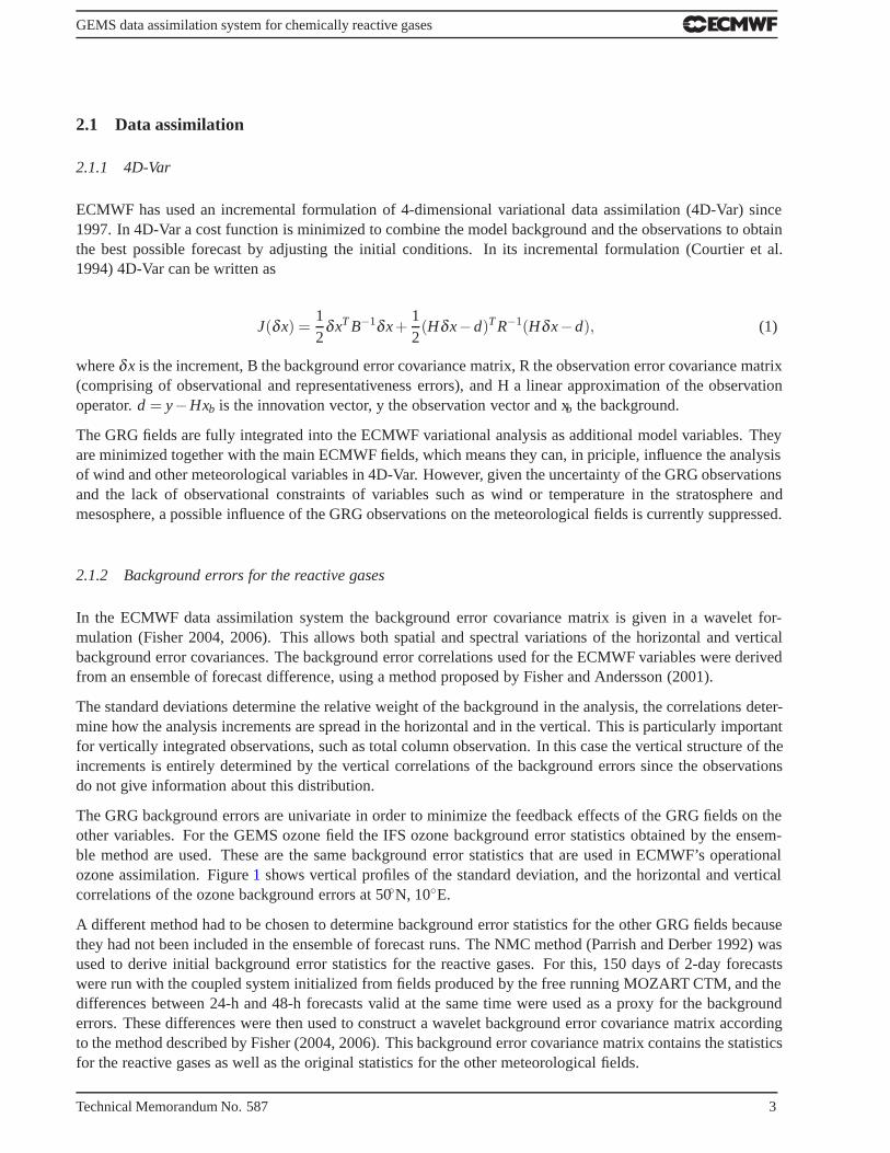
Figure 7: Ozone cross section from 40◦S across the South Pole back to 40◦S along 8◦E from GRGAN (top left) and GRGCTRL (topright) on 4 October 2003, 12z. The bottom panel shows ozone profiles at the Neumayer station (71◦S, 8◦E) from an ozone sondelaunched on 4 October 2003 (red), GRGAN (black) and GRGCTRL (orange). The Unit is mPa.

is a representativeness error and the model with a horizontal resolution of T159 (corresponding to a reducedGaussian grid of about 125 km x 125 km) is not able to reproduce the high values observed by MOZAIC overboth airports. Alternatively, it could be a sign that the surface CO emissions used by the MOZART CTM aretoo low to reproduce the high CO values observed by MOZAIC in the lower troposphere.

3.3 NO2 assimilation

To test the assimilation of NO2 data with the coupled GEMS system, first a single observation experiment iscarried out. For a single total column observation the shape of the analysis increment is given by BHt . Fordiagonal B and R matrices this gives

H(xa − xb) = HBHt(HBHt +R)−1(y−Hxb) = σ 2b (

y−Hxb

σ 2b + σ 2

o), (3)

where xa is the analysis value, xb the background value, y the observation, H is the observation operator, B thebackground error covariance matrix, R the observation error covariance matrix, σ2

b the observation equivalent



St. dev. and bias OB-FG OB-AN

-0.18-0.12-0.06

00.060.120.180.240.300.36

MAY2003


MAY2003


1 122915 26 10 24 7 21 4 18 2 133016 27 11 25

1 122915 26 10 24 7 21 4 18 2 133016 27 11 25

� 4 days MA

3600

4800

6000

7200

8400

9600

10800

Daily used observations

Figure 8: Timeseries of globally averaged MOPITT total column CO first-guess departures (red dotted line) and analysis departures(blue dotted line), as well as standard deviations of first-guess departures (red solid line) and of analysis departures (blue solid line) in1018mol/cm2 (top panel), and number of observations per assimilation cycle (bottom panel) from GRGAN for used data.

of the background covariance and σ2o the observation variance.

To investigate how the increment from one NO2 observation is spread out in the vertical and horizontal, a singletropospheric column NO2 observation is placed at 38.6◦N, 119.3◦E on 2 January 2006, 02:32:20 hours. Theobservation has a value of 28.8x1015 mol/cm2 and an error of 20%. It is 19.1x1015 mol/cm2 higher than thebackground. Averaging kernels for the observation are used in the observation operator. No variational qualitycontrol and first-guess checks are applied.

Figure 11 (top left panel) shows the total column NOx increment resulting from the assimilation of this ob-servation. The NOx increment has a maximum value of 16.3x1015 mol/cm2 at the location of the observation.The first-guess NO2 value at the location of the observation is 9.7x1015 mol/cm2 and the analysis NO2 value14.1x1015 mol/cm2.

The top right panel of Figure 11 shows a vertical cross section through the analysis increment along 119.3◦E.The impact of the observation is confined to the lowest five model levels. The absolute impact is largest aroundmodel level 57. The bottom panel of Figure 11 shows the vertical NOx analysis and first-guess profiles at thelocation of the observation and illustrates again how the analysis increment is distributed in the vertical.

A 1-month long NO2 assimilation experiment (NO2AN) is run with the coupled GEMS system for January



00.40.81.21.622.42.83.23.64

-1-0.5-0.375-0.25-0.12500.1250.250.3750.51

00.40.81.21.622.42.83.23.64

-1-0.5-0.375-0.25-0.12500.1250.250.3750.51

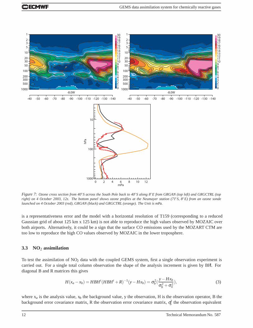
Figure 9: Mean total column CO field averaged over the seasons JJA (top) and SON (bottom) 2003. The left panels show GRGAN,the right panels the difference between GRGAN and GRGCTRL (GRGAN minus GRGCTRL). Unit is 1018 molecules/cm2.

2006. The NO2 data used in the assimilation experiment are tropospheric NO2 columns from SCIAMACHY,derived by KNMI with a DOAS algorithm (http://www.gse-promote.org). The retrieval method and an erroranalysis of the retrieval are given in Boersma et al. (2004). The data have large errors in clean areas, dominatedby errors in the spectral fitting and stratospheric column estimate. Over continental areas the error is of theorder 35-60%. Best results are obtained in regions with strong NO2 sources or high surface albedo. Areas withtropospheric column values greater than 1.0x1015 mol/cm2 have errors of less than 50%. The data producersprovide averaging kernels with the data, and this information is used in the observation operator for the as-similation. In addition to NO2AN a control experiment is run in which the SCIAMACHY NO2 data are onlyincluded passively (NO2CTRL).

Figure 12 shows monthly mean tropospheric NOx columns (integral between model levels 35 and 60) fromNO2AN for January 2006, the difference between the monthly mean tropospheric NO2 column from NO2ANand NO2CTRL, as well as monthly mean tropospheric NO2 values from OMI (note the different colour scales).The OMI data are independent data that were not used in the analysis. The analysis gives a realistic NOxfield with high NOx values over North America, Europe, India and South-East Asia. It also shows up biomassburning areas in tropical Africa and elevated NOx values over several cities in the SH. The control run hashigher NOx concentrations almost everywhere, with the exception of some biomass burning areas in Africa,and some pollution hot spots over Beijing, and several Indian cities.

Figure 13 shows a timeseries of globally averaged NO2 tropospheric column first-guess and analysis departuresfrom NO2AN and their standard deviations, as well as the number of observations per analysis cycle. Plottedare statistics for data that are actively used in the analysis in January 2006. The timeseries shows that theanalysis is drawing to the data, and that departures and their standard deviations are reduced. However, a smallbias (dotted lines) remains in the analysis, and the differences between the standard deviations of the first-guessand analysis departures are not as large as the ones seen for the CO assimilation (Figure8). This suggests thateither the background errors for NOx are too tight, or that because of the larger observation errors of the NO2

data a smaller correction is carried out by the analysis.

The spikes seen in Figure 13 on 8, 11, 15, and 27 January, 0z, are due to high observed NO2 values over



100 150 200ppb

250 300 100 150 200ppb

250 300 100 200 300ppb

400 500

0 200ppb400 600 10050 150 200

ppb250 300 100 200 300

ppb400 500

hPa

200

300

400

500

600700800900

1000

hPa

200

300

400

500

600700800900

1000

hPa

200

300

400

500

600700800900

1000

hPa

200

300

400

500

600700800900

1000

hPa

200

300

400

500

600700800900

1000

hPa

200

300

400

500

600700800900

1000

Figure 10: Monthly mean CO profiles over Frankfurt (top panels) and Osaka (bottom panels) from GRGAN (black), GRGCTRL (blue)and independent MOZAIC data (red) for September (left panels), October (middle panels), and November 2003 (right panels) in ppb.The solid lines show the mean profiles, the dotted lines +/- one standard deviation.

South East Asia. An example is given in Figure 14 that shows the analyzed tropospheric NOx column fromNO2AN and NO2CTRL on 20060111, 0z, their difference (NO2AN minus NO2CTRL), and the troposphericNO2 columns from SCIAMACHY that were used in the analysis. The observations show high NO2 values overChina, Japan and North-East India, and the analysis reproduces these high values well. The control run haslower NOx concentrations over the polluted areas than the analysis, but higher background concentrations.

The examples shown here indicate that the NO2 analysis is working well. A more detailed validation study willhave to be carried out, including a thorough comparison with independent NO2 observations.

3.4 HCHO assimilation

To test the assimilation of HCHO data with the coupled GEMS system, first a single observation experiment iscarried out. A single total column HCHO observation is placed at 49.4◦N, 136.4◦E on 1 July 2006, 01:31:18hours. The observation has a value of 30x1015 mol/cm2 and an error of 20%. It is 15.7x1015 mol/cm2 higherthan the background. Averaging kernels for the observation are used in the observation operator. No variational



35°N

40°N

45°N

110°E 120°E60°N 56°N 52°N 48°N 44°N 40°N 36°N

36

40

44

48

52

56

60

32°N 28°N 24°N 20°N

2

4

6

8

10

12

14

16

18

119.3E1

4

8

12

16

20

24

28

32

36

40

5 10 15 20 25 30 35 40

36

40

44

48

52

56

60

Figure 11: Tropospheric column (integral between model levels 35 and 60) NOx analysis increment (top left) in 1015mol/cm2, verticalcross section of analysis increment at 119.3◦E in ppb (top right), and NOx analysis (solid) and first-guess (dashed) profiles in ppb(bottom) from a single NO2 tropospheric column observation placed at 38.6◦N, 119.3◦E on 20060102, at 02:32:20 hours.

quality control and first-guess checks are applied. Figure15 (top left panel) shows the total column incrementresulting from the assimilation of this observation. The increment has a maximum value of 4.4x1015 mol/cm2

at the location of the observation. The first-guess value at the location of the observation is 14.3x1015 mol/cm2

the analysis value is 18.7x1015 mol/cm2. The magnitude of the increment agrees with what is expected fromtheoretical arguments (Equation 3).

The top right panel of Figure 15 shows a vertical cross section through the analysis increment along 136.4◦E.The absolute impact of the observation is largest around model level 55. However the impact of the observationcan be seen throughout the troposphere (up to level 30). The bottom panel of Figure15 shows the verticalHCHO analysis and first-guess profiles at the location of the observation and illustrates again how the analysisincrement is distributed in the vertical.

A 1-month long HCHO assimilation experiment (HCHOAN) is run with the coupled GEMS system for August2008. The HCHO data used in HCHOAN are total column HCHO data produced by the Belgian Institutefor Space Aeronomy (BIRA) for the PROMOTE project (http://www.gse-promote.org). Information about theretrieval and the data quality can be found in De Smedt et al. (2006). Monthly mean HCHO values have totalerrors of 20-40%, individual pixels have much larger total errors, dominated by the random error. Because thetotal error of the data increases with latitude, only data between 50◦N and 50◦S are used in GRGAN. Data witha cloud fraction greater than 40% are also rejected, and no data are used over the area of the South AtlanticAnomaly. The data producers provide averaging kernels with the data, and this information is used in the



0.512345681015

-20-10-5-1-0.500.5151020

0 1 2 3 4 6 8 11 15 20

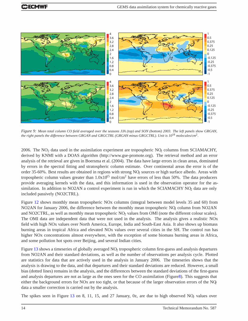
Figure 12: Tropospheric NOx columns (integral between model levels 35 and 60) from NO2AN (top left), difference between NO2ANand NO2CTRL (top right), and monthly mean tropospheric NO2 from OMI (bottom panel). Unit is 1015mol/cm2. The OMI plot wastaken from http://www.gse-promote.org/.

observation operator for the assimilation. Because of the noise in the data, it is not ideal to use the data for anassimilation experiment. They would be better suited to monthly mean validation studies. However, becauseno other HCHO data are available, the data are used in HCHOAN despite their shortcomings.

Figure 16 shows a timeseries of globally averaged HCHO tropospheric column first-guess and analysis depar-tures and their standard deviations for August 2007, as well as the number of observations used per analysiscycle. Plotted are statistics for data that are actively used in the analysis. The timeseries shows that the analysisis drawing to the data and that bias and standard deviation of the departures are reduced. However, a consider-able bias remains and the standard deviation of the analysis departures remains large, indicating that there is alot of noise in the data.

Figure 17 shows the monthly mean total column HCHO field from HCHOAN for August 2007, the monthlymean difference between HCHOAN and HCHOCTRL and the monthly mean total column HCHO field fromindependent OMI data (note the different colour scales). The analysis produces a realistic looking total columnHCHO field that agrees well with the independent OMI data. The assimilation leads to increased HCHO valuesover the oceans and reduced values over land.

These first results show that the assimilation of HCHO data with the coupled GEMS system is working inprinciple. However, better quality data are needed if HCHO data are to be assimilated in longer reanalysis runswith the GEMS system.

3.5 SO2 assimilation

The coupled system will only be used to assimilate SO2 observations for case studies of volcanic eruptions. Asan example, the eruption of Mount Nyamuragira in central Africa in 2006 is presented here. Nyamuragira began



1234567

JAN 20061 4 7 10 13 16 19 28 312522

JAN 20061 4 7 10 13 16 19 28 312522

30003600420048005400600066007200780084009000

4 days MADaily used observations


Figure 13: Timeseries of globally averaged SCIAMACHY tropospheric column NO2 first-guess departures (red dotted line) andanalysis departures (blue dotted line), as well as standard deviations of first-guess departures (red solid line) and analysis departures(blue solid line) in 1015mol/cm2 (top panel), and number of observations per assimilation cycle (bottom panel) from NO2AN for useddata for January 2006.

erupting on 27 November 2006 around 10pm local time, and SO2 emissions were observed by the OMI instru-ment until 4 December (see http://so2.umbc.edu/omi/ and http://earthobservatory.nasa.gov/IOTD/view.php?id=7189.).The OMI observations show that the SO2 plume first travelled westward, then moved in a clockwise directiontowards the northeast, and eventually reached India (see Figure18).

For the SO2 assimilation experiment of the Nyamuragira eruption (SO2AN) total column SO2 retrievals fromSCIAMACHY are used that were produced by BIRA for the PROMOTE project (http://www.gse-promote.org).Information about the retrieval and the data quality can be found on the PROMOTE website. BIRA producethree different vertical column density retrievals, for three different assumed plume heights (1 km above ground,6 km, and 14 km). Here, the BIRA retrieval that assumes a plume height of 6km is used, and a SO2 JB thatpeaks at 6 km (see Figure 4) for first assimilation tests. Unfortunately, no SCIAMACHY data are availableover Africa between 28-30 November, so that SO2AN is only started on 1 December, 0z, three days after thevolcanic eruption began. SO2 data are only assimilated in the area between 30◦N and 30◦S, 0◦ and 40◦E andblacklisted elsewhere.

Figure 19 shows maps of total column SO2 in Dobson Units from SO2AN. The background forecast (top left)shows elevated SO2 concentrations over North America, Europe, Russia, India and China. The backgroundforecast does not show any elevated SO2 values over Africa, because the MOZART CTM that provides theinitial SO2 field does not know about the Nyamuragira eruption. By assimilating the SCIAMACHY SO2 data



012345681020200

012345681020200

-200-50-10-5-10151050200

012345681020200

Figure 14: Tropospheric NOx columns (integral between model levels 35 and 60) from NO2AN (top left), NO2CTRL (top right),difference between NO2AN and NO2CTRL (bottom left), and SCIAMACHY tropospheric NO2 columns (bottom right) that were used inthe assimilation on 20060111, 0z. Unit is 1015mol/cm2.

(Figure 19 top right panel) this information is brought into the analysis (middle left). The plume then spreadsnorth westwards and eventually eastwards in the NH and to a lesser extent into the SH. It reaches India andAustralia by 3 December (bottom left), and NH central Pacific by 6 December (bottom right). Our analysisvalues are lower than the values observed by OMI (see Figure18), but on the whole our SO2 analysis patternsagree well with the OMI observations (Figure 18). The maximum values of the assimilated SCIAMACHY SO2

data are lower than those of the OMI data, probably because of the larger pixel sizes and bigger data gaps ofSCIAMACHY.

Figure 20 shows area averaged SO2 profiles from SO2AN for an area over Africa (left panel) and a cleanarea over the north-west Pacific (right panel) on 1, 3, and 6 December 2006. The Africa profiles show largeSO2 values in the middle troposphere where the assimilation places the bulk of the volcanic SO2. It alsoshows how the SO2 concentrations spread out in the vertical with time, as SO2 is transported by the model.SO2 concentrations decrease after the eruption between 3 and 6 December, but even on 6 December maximumvalues are still greater than 10 ppb. The profiles over the clean area over the north-west Pacific show an increasein SO2 concentrations on 3 and 6 December, because SO2 from the volcanic eruption has been transported here.Overall the SO2 concentrations in the clean area are a factor of 10 lower on 6 December than over Africa.

These first results from the assimilation of SO2 data are encouraging. The coupled system manages to reproducerealistic SO2 patterns if SCIAMACHY SO2 data are assimilated, even if there are no volcanic emissions in thebackground model. It has to be kept in mind that the vertical structure of the analyzed SO2 field entirely dependson the background error covariances, which in this case prescribe an injection height of 6km. The case studywill be repeated when OMI SO2 data are available for that period, because OMI has a better data coverage andalso provides data for the first three days after the eruption.



45°N

50°N

55°N

130°E 140°E0.5

1

1.5

2

2.5

3

3.5

4

4.5

60

50

40

30

20

10

0.125

0.25

0.375

0.5

0.625

0.75

0.875

1

1.125

1.5

68°N 64°N 60°N 56°N 52°N 48°N 44°N 40°N 36°N 32°N

60

50

40

30

20

10

1 2

Figure 15: Total column HCHO analysis increment (top left) in 1015mol/cm2, vertical cross section of analysis increment at 136.4◦Ein ppb (top right), and HCHO analysis (solid) and first-guess (dashed) profiles in ppb (bottom) from a single HCHO observation placedat 49.4◦N, 136.4◦E on 20060701, at 01:31:18 hours. The observation has a value of 30x1015 mol/cm2 and an error of 20%, and is15.7x1015 mol/cm2 higher than the background.

4 Conclusions and outlook

A data assimilation system for the chemically reactive gases O3, CO, NOx, HCHO, and SO2 has been developedas part of the EU funded GEMS project, by coupling the three CTMs MOZART, MOCAGE and TM5 toECMWF’s IFS using the OASIS4 coupler. In this paper, the GEMS GRG assimilation system was describedand some first results were shown that were obtained with the coupled system where the MOZART CTM wascoupled to IFS. The background error statistics for O3 were obtained with the analysis ensemble method, thebackground error statistics for CO, NOx and HCHO were based on the NMC method. Background errors forSO2 were prescribed to mimic the deposit of volcanic SO2 in the free troposphere. Assimilation experimentswere carried out for all five species, assimilating O3 retrievals from SCIAMACHY, MIPAS, GOME and SBUV,CO retrievals from MOPITT, and NO2, HCHO and SO2 retrievals from SCIAMACHY. Results from theseassimilation experiments illustrate that the coupled approach is working successfully and that the reactive gasesassimilation system gives realistically looking results.

It is planned to carry out more comprehensive validation studies against independent observations for assimi-lation experiments of all five species and to present these in future studies. Further effort will also be spent onimproving the coupled system. The CTMs are constantly improved, and these improvements will be includedin the coupled system. Aspects of the data assimilation system will also be refined. For example, it is planned torecalculate the background error statistics for the reactive gases with the NMC method using a newer version ofthe coupled system, and in the longer term the analysis ensemble method will be used to calculate new statistics



12345678

3000360042004800540060006600720078008400

AUG 20071 4 7 10 13 16 19 28 312522

AUG 20071 4 7 10 13 16 19 28 312522

4 days MADaily used observations


Figure 16: Timeseries of global mean SCIAMACHY tropospheric column HCHO first-guess departures (red dotted line) and analysisdepartures (blue dotted line), as well as standard deviations of first-guess departures (red solid line) and analysis departures (bluesolid line) in 1015mol/cm2 (top panel), and number of observations per assimilation cycle (bottom panel) from HCHOAN for used datafor August 2007.

for the GRG fields. A bias correction scheme is being developed for the GRG fields and will be used in futurestudies.

The coupled assimilation system was used in collaboration with the greenhouse gas and aerosol subprojectsof GEMS to carry out a 5-year long reanalysis of atmospheric composition data for the period 2003-2007,assimilating satellite data to constrain O3, CO, CO2, CH4, and aerosol optical depth. It is also being used fora near-real time analysis of O3, CO and aerosol optical depth that is being run at ECMWF. Fields from theseanalyses are available from http://gems.ecmwf.int/data.jsp

5 Acknowledgements

GEMS was funded by the European Commission under the EU Sixth Research Framework Programme, con-tract number SIP4-CT-2004-516099.



0369121518212427304050

-5

-2.5

-1

-0.5

0

0.5

1

2.5

5

Figure 17: Monthly mean total column HCHO field in 1015mol/cm2 from HCHOAN (top left) andthe difference between HCHOAN and HCHOCTRL (HCHOAN minus HCHOCTRL) (top right) for August2007. The bottom panel shows the monthly mean total column HCHO field from OMI, obtained fromhttp://www.cfa.harvard.edu/ tkurosu/SatelliteInstruments/OMI/SampleImages/HCHO/index.html.

6 References

Atkinson, R. (1994): Gas-phase tropospheric chemistry of organic compounds. J. Phys. Chem. Ref. DataMonogr., 2, 13-46.

Benedetti et al. (2009): Aerosol analysis and forecast in the ECMWF Integrated Forecast System: Data assim-ilation, submitted to J. Geophys. Res..

Boersma, K.F., Eskes, H.J., and Brinksma, E.J. (2004): Error analysis for tropospheric NO2 retrieval fromspace.J. Geophys. Res., 109, D04311, doi:10.1029/2003JD003962.

Cariolle, D. and Deque, M. (1986): Southern hemisphere medium-scale waves and total ozone disturbances ina spectral general circulation model. J. Geophys. Res., 91D, 1082510846.

Courtier, P., Thepaut, J.-N. and Hollingsworth, A. (1994): A strategy for operational implementation of 4D-Var,using an incremental approach. Q. J. R. Meteorol. Soc., 120, 1367-1388.

Crutzen, P., and Schmailzl, U. (1983): Chemical budgets of the stratosphere, Planet. Space. Sci., 31, 1009-1020.

Deeter et al. (2003): Operational carbon monoxide retrieval algorithm and selected results for the MOPITTinstrument. J. Geophys. Res., 108(D14), 4399, doi:10.1029/2002JD003186

Dethof, A. and Holm, E.V (2004): Ozone assimilation in the ERA-40 reanalysis project. Quart . J. Roy. Met.Soc., 130, 2851-2872.

De Smedt, I., M”uller, J.F., Stavrakou, T., van der A, R., Eskes, H, and Van Roozendael, M. (2008): Twelve



0

-5

0

5

10

15

20

25

10 20 30 40 50 60 70 80

0

-5

0

5

10

15

20

25

10 20 30 40

5 6 7 8 9 100 1 2 3 4

50 60 70 80

0

-5

0

5

10

15

20

25

10 20 30 40 50 60 70 80

Figure 18: Total column SO2 field in Dobson Units from OMI on 1, 3, and 6 December 2006. The plots were taken from the OMISulfur Dioxide Group website http://so2.umbc.edu/omi/.

years of global observations of formaldehyde in the troposphere using GOME and SCIAMAHCY sensors.Atmos. Chem. Phys., 8, 4947-4963.

Elguindi, N. et al. (2009): Improvment of the global distribution and long-range transport of tropospheric COby using the IFS-ECMWF model coupled to a free CTM with CO MOPITT assimilation. In preparation.

Engelen R. J., S. Serrar, F. Chevallier (2009), Four-dimensional data assimilation of atmospheric CO2 usingAIRS observations, J. Geophys. Res., 114, D03303, doi:10.1029/2008JD010739.

Granli, T., and Bokman, O. (1994): Nitous oxides from agriculture, Nor. J. Acric. Sci., 12, 1-128.

Hansen, J., M. Sato, and R. Ruedy (1997): Radiative forcing and climate response, J. Geophys. Res., 102,68316864.

Hollingsworth, A., R.J. Engelen, C. Textor, A. Benedetti, O. Boucher, F. Chevallier, A. Dethof, H. Elbern, H.Eskes, J. Flemming, C. Granier, J.W. Kaiser, J.J. Morcrette, P. Rayner, V.H. Peuch, L. Rouil, M.G. Schultz, A.J.Simmons, and The GEMS Consortium (2008): Toward a Monitoring and Forecasting System For AtmosphericComposition: The GEMS Project. Bull. Amer. Meteor. Soc., 89, 11471164, doi:10.1175/2008BAMS2355.1

Holm, E. V., Untch, A., Simmons, A., Saunders, R., Bouttier, F. and Andersson, E. (1999): Multivariateozone assimilation in four-dimensional data assimilation. Pp. 89-94 in Proceedings of the SODAWorkshop onChemical Data Assimilation, 9-10 December 1998, KNMI, De Bilt, The Netherlands.

Horowitz, L. W., Walters, S., Mauzerall, D.L., Emmons, L.K., Rasch, P.J., Granier, C., Tie, X., Lamarque,J.F., Schultz, M.G., Tyndall, G.S., Orlando, J.J. and Brasseur, G.P. (2003): A global simulation of tropo-spheric ozone and related tracers: Description and evaluation of MOZART, version 2, J. Geophys. Res.,doi:10.1029/2002JD002853.

Josse B., Simon P. and V.-H. Peuch (2004) : Rn-222 global simulations with the multiscale CTM MOCAGE,



0.10.20.5125102050

0.10.20.5125102050

0.10.20.5125102050

0.10.20.5125102050

0.10.20.5125102050

0.10.20.5125102050

Figure 19: Total column SO2 field in Dobson Units from SO2AN. Background forecast for 1 Dec, 0z (top left), SCIAMACHY observa-tions that are assimilated in SO2AN on 1 Dec, 0z (top right), SO2 analysis for 1 Dec, 0z (middle left), 1 Dec, 12z (middle right), 3 Dec,12z (bottom left) and for 6 Dec, 12z (bottom right).



60

50

40

30

20

10

0 4 8 12 16 20 24 28 3260

50

40

30

20

10

0 0.1 0.2 0.3 0.4 0.5 0.6 0.7 0.8 0.9

Figure 20: Profiles of SO2 in ppb averaged over the area between 20◦N and 20◦S, 0◦ and 50◦E (left) and over the area between30-40◦N, 160-180◦E (right), on 20061201, 0z (black), 20061203, 12z (red) and 20061206, 12z (blue).

Tellus, 56B, 339-356.

Fisher, M. and Andersson, E. (2001): Devlopments in 4D-Var and Lalman Filterning. ECMWF TechnicalMemorandum 347. Available from ECMWF, Shinfield Park, Reading, Berkshire, RG2 9AX, UK.

Fisher, M. (2004): Generalized frames on the sphere with application to background error covariance modellig.Seminar on resent developments in numberical methods for atmospheric and ocean modelling, 6-10 September2004. Proceedings, ECMWF, pp. 87-101. Available from ECMWF, Shinfield Park, Reading, Berkshire, RG29AX, UK.

Fisher, M. (2006): Wavelet Jb - A new way to model the statistics of background errors. ECMWF Newsletter,106, 23-28. Available from ECMWF, Shinfield Park, Reading, Berkshire, RG2 9AX, UK.

Flemming, J., Inness, A., Flentje, H., Huijen, V., Moinat, P., Schultz, M.G. and Stein O. (2009): Couplingglobal chemistry transport models to ECMWF’s integrated forecast system for forecast and data assimilation.ECMWF Technical Memorandum 590. Available from ECMWF, Shinfield Park, Reading, Berkshire, RG29AX, UK.

Hortal, M. and Simmons, A.J. (1991): Use of reduced Gaussian grids in spectral models. Mon. Wea. Rev.,119, 1057-1074

Kanakidou, M., and P. J. Crutzen (1999): The photochemical source of carbon monoxide: Importance, uncer-tainties, and feedbacks, Chemosphere Global Change Sci., 1, 91109.

Kinnison, D.E., Brasseur, G.P., Walters, S., Gracia, R.R., Marsh, D.R., Sassi, F., Harvey, V.L., Randall, C.E.,Emmons, L., Lamarque, J.F., Hess, P., Orlando, J.J., Tie, X.X., Randel, W., Pan, L.L., Gettelman, A., Granier,C., Diehl, T., Niemeier, U. and Simmons, A.J. (2007): Sensitivity of chemical tracers to meteorological parame-ters in the MOZART-3 chemical transport model. J. Geophys. Res, 112, D20302, doi:10.1029/2006JD007879.

GEMS GRG validation report (2009). Available from http://gems.ecmwf.int/documents/index.jsp.

Kleinman, L., Y.-N. Lee, S. R. Springston, J. H. Lee, L. Nunnermacker, J. Weinstein-Lloyd, X. Zhou, andL. Newman (1995): Peroxy radical concentration and ozone formation rate at a rural site in the southeasternUnited States, J. Geophys. Res., 100(D4), 7263-7274.

Krol, M.C.,and van Weele, M. (1997): Implications of variations in photodissociation rates for global tropo-spheric chemistry, Atmospheric environment, 31, 1257-1273.



Krol, M.C., S. Houweling, B. Bregman, M. van den Broek, A. Segers, P. van Velthoven, W. Peters, F. Dentener,and P. Bergamaschi The two-way nested global chemistry-transport zoom model TM5 (2005): algorithm andapplications Atmos. Chem. Phys., 5, 417-432.

Landgraf, J. and P.J. Crutzen (1998): An efficient method for online calculations of photolysis and heatingrates. J. Atmos. Sci., 55, 863-878.

Logan, J. A., M. J. Prather, S. C. Wofsy, and M. B. McElroy (1981): Tropospheric chemistry: A global per-spective, J. Geophys. Res., 86, 72107254.

Lopez, P. and Moreau, E. (2005): A convection scheme for data assimilation: Description and initial tests,Quarterly Journal of the Royal Meteorological Society, 131, 606, p 409-436.

Martin, R. V., B. Sauvage, I. Folkins, C. E. Sioris, C. Boone, P. Bernath, and J. Ziemke (2007): Space-basedconstraints on the production of nitric oxide by lightning, J. Geophys. Res., 112, D09309, doi:10.1029/2006JD007831.

National Research Council (NRC) (1991): Rethinking the Ozone Problem in Urban and Regional Air Pollution,Natl. Acad. Press, Washington, D. C..

Nedelec, P. et al. (2003): An improved infrared carbon monoxide analyser for routine measurements aboardcommercial aircraft: technical validation and first scientific results ofr the MOZAIC III programme, Atmos.Chem. Phys., 3, 1551-1564.

Ordonez, C. et al. (2009): Global model simulations of air pollution during the European 2003 heat wave. Inpreparation.

Parrish, D.F. and J.C. Derber (1992): The National Meteorological Center’s spectral statistical-interpolationanalysis scheme. Mon. Weather Rev., 120, 1747-1763

Pham, M., Muller, J.-F., Brasseru, G.P., Garnier, C, and Megie, G. (1996): A 3D model study of the golbalsulphur cycle: Contibutions fo anthropogenic and biogenic sources, Atmos. Environ., 30, 1815-1822.

Seinfeld, J. H., and S. N. Pandis (2006): Atmospheric Chemistry and Physics: From Air Pollution to ClimateChange, John Wiley, Hoboken, N. J.

Stein, O. (2009): Model documentation of the MOZART CTM as implemented in the GEMS system. Availablefrom: http://gems.ecmwf.int/documents/index.jsp#grg.

Valcke, S. and Redler, R. (2006): OASIS4 User Guide (OASIS4 0 2). PRISMSupport Initiative, TechnicalReport No 4. Available from http://www.prism.enes.org/Publications/index.php.


Documents

GEMS data assimilation system for chemically reactive gases