University of Groningen Groningen Growth and Development Centre

Measurement error in cross-country productivity comparisons:Is more detailed data better? Research Memorandum GD-111 Robert Inklaar and Marcel Timmer RESEARCH MEMORANDUM

Measurement error in cross-country productivity comparisons:

Is more detailed data better?

Robert Inklaar and Marcel P. Timmer University of Groningen

March 2009

Abstract: Relative productivity levels are used intensively in analyzing cross-country growth, but often based on crude measures and with little information on their reliability. In this paper, we provide a new framework to estimate purchasing power parities and productivity levels with associated standard errors using the country-product-dummy (CPD) method. For a set of OECD countries, we show that productivity levels in manufacturing industries are measured with sizeable error. We also show that cruder productivity measures are often poor proxies for the data-intensive measure presented here. This evidence can be used to deal with the problem of attenuation bias in cross-country regressions. JEL classification: C43, E01, O14, O47. Keywords: Measurement error; Index numbers; Productivity levels; Manufacturing.

1

1. Introduction Measurement error in productivity levels has long been a concern in cross-country studies of economic growth. But so far, little is known about its relative importance as estimates of these errors are lacking. This problem is increasingly pressing due to the increased use of productivity levels as an explanatory variable in recent years. This reinforces the need for better measures of relative productivity and a systematic approach to estimating measurement error.1 In this paper, we aim to develop such an approach.

Relative productivity is a key variable in the new endogenous growth models that are focused on the generation and diffusion of technology and knowledge across countries. Relative productivity, or the “distance to the frontier,” measures the potential for international technology transfer: when a country approaches the world technology frontier, there is less room for adoption of existing technologies and innovation becomes more important for generating growth. Following the seminal study by Griffith, Redding and van Reenen (2004), various studies have shown that the impact of R&D expenditures, skill level of the labor force, openness to international trade and degree of market regulation on growth depend crucially on a country’s distance to the frontier. The proxy for this distance is the level of multifactor productivity (MFP) in a country relative to the highest MFP level in the sample of the countries studied.2

Until recently, these studies had to rely on the rather crude measures of productivity that have become standard since the work of Bernard and Jones (1996). A typical measure of productivity in say manufacturing would be based on nominal value added converted with a PPP (purchasing power parity) for aggregate GDP, and total number of workers and capital stock as measures of labor and capital input respectively. It is well recognized that the use of such crude productivity measures can be misleading. Production theory has shown that accurate measures of productivity require detailed information about prices and quantities of many types of inputs (Jorgenson, 1995). Additionally, various studies stress the importance of having appropriate industry-level PPPs to compare value added (Bernard and Jones, 2001).3

Fortunately, the availability of detailed data to improve international level comparisons is steadily increasing. Various studies break down investment flows by type of asset, and provide data on employment of different types of workers classified by educational attainment.4 Recently, a comprehensive database was released that provides internationally harmonized measures of output, input and productivity for 30 advanced countries based on a

1 An early example is the comment of De Long (1988) on Baumol (1986). Durlauf, Johnson and Temple (2005) provide a recent overview. 2 Recent applications include Griffith, Redding and van Reenen (2004) on the effects of R&D; Vandenbussche, Aghion and Meghir (2006) for the effects of university education; Cameron, Proudman and Redding (2005) for the effects of international trade; Nicoletti and Scarpetta (2003) and Inklaar, Timmer and van Ark (2008) for the effects of product market regulation. Acemoglu, Aghion and Zilibotti (2006) and Aghion and Howitt (2009) provide theoretical background. 3 See also Sørenson (2001), Acemoglu and Zilibotti (2001), Caselli (2005) and Rogerson (2008). 4 De la Fuente and Doménech (2006) and Cohen and Soto (2007) provide growth and convergence studies based on detailed measures of labor input. Caselli and Wilson (2004), Jorgenson and Vu (2005) and Timmer and van Ark (2005) provide country-wide comparisons of productivity allowing for different types of capital, in particular ICT-capital, while Hsieh and Klenow (2007) highlight the importance of differences in relative prices of various asset types.

2

variety of detailed national sources, including national accounts data, production and investment surveys and various labor force statistics. This has been complemented by a set of industry-level PPPs that allow for comparisons of both levels and growth rates of productivity across a wide set of countries.5

Although these new measures are considered to be conceptually superior, productivity measures based on more detailed data may well have sizeable measurement errors. There are various reasons to believe this is the case. For example, while an estimate of total workers in an industry can be made relatively precisely, estimates of hours worked by university-educated workers are much more uncertain. Typically these measures are based on additional survey data with a limited sample size, such as Labor Force Surveys, so looking at more detailed categories of workers tends to increase sampling error. Similarly, aggregate investment by asset type is normally available from the National Accounts. However, the allocation of assets to using industries is much less reliable than the aggregate series and depends on a wide variety of assumptions and scattered evidence. More generally, estimates based on sectoral data are less reliable due to sampling, reporting or other errors, while estimates based on aggregate data are more robust as errors tend to be averaged out (Griliches, 1986; Diewert, 2001).6

So far, there have been two basic approaches to dealing with measurement error in the growth literature. The standard approach is to test whether the main results of a study based on crude measures are robust to various data refinements. Implicitly this strategy assumes that more data-intensive measures are alternatives for crude measures and leaves unanswered the question whether the data-intensive measures are merely different, or whether they are better in any sense. Without an answer to this, conflicting outcomes based on crude and sophisticated measures cannot be dealt with.7 Another approach is to recognize that measurement error will lead to an attenuation bias of the parameter estimate.8 Researchers can then use reverse regression or method-of-moments estimators to test the robustness of their results (Temple, 1998). So far, these techniques have not been used routinely in applied growth research. One reason is that they require information about the likely extent of measurement error that is currently not available. As a result, one has to rely on educated guesses that provide some likely upper and lower bounds. Another regression technique to correct for measurement error is to use instrumental variables. In practice, this requires using lagged productivity levels as instruments (Griffith, et al., 2004) but the data need to satisfy strong restrictions for this approach to be valid. Instead, most growth studies choose to ignore possible measurement error in their productivity level estimates (Durlauf, Johnson and Temple, 2005).

5 Data in national prices are provided in the EU KLEMS database, see O’Mahony and Timmer (2009) for an overview. Industry-level PPPs are provided in Inklaar and Timmer (2009). 6 For example, see the discussion of the findings in Inklaar, Timmer and van Ark (2008) by Wendy Carlin, Jonathan Temple and a panel (Inklaar et al, 2008, p.171-78). 7 For examples of this strategy, see the studies in footnote 2. Conflicting evidence is found by Inklaar et al. (2008). Based on data-intensive measures they could not corroborate the findings by Vandenbussche et al. (2006) which were based on crude productivity measures. 8 Attenuation bias, where the true coefficient is larger than the OLS estimate, occurs if only one variable in a regression is measured with error. In the more general case where all variables are measured with error, the true parameter may be larger or smaller than the OLS estimate; see Klepper and Leamer (1984).

3

The objective of this paper is to investigate empirically the nature and extent of errors of measurement in productivity level estimates. This is potentially useful for improving empirical strategies used in cross-country growth research. We develop a coherent regression framework in which estimates of productivity levels can be derived together with estimates of their standard error. This is the first study to so, relying on a dual representation of productivity as a ratio of output and input PPPs. We find evidence that measurement error in more data-intensive estimates is indeed substantial and positively correlated with the technological sophistication of the industry. Our results also show that the standard, cruder measures are poor proxies for the conceptually more appealing data-intensive measures. Using the cruder measures in regression analysis would therefore lead to biased results. An adjustment for hours worked and the relative skill level of the labor force would already greatly improve the estimates of productivity levels but if this were the only adjustment, models in which the interaction with the distance to the frontier is an explanatory variable would still be biased.

These results can also be useful for studies outside the endogenous growth literature. Levels of productivity are key in recent models of structural change and employment (Rogerson, 2008) and used by Acemoglu and Zilibotti (2001) to study the impact of skill-technology complementarity on international income differences. They figure prominently in studies explaining patterns of international trade and comparative advantage, and are the cornerstone of explanations of the Harrod-Balassa-Samuelson effect which states that more productive economies exhibit higher average prices relative to their trading partners.9 In particular, the recent development of models of trade and macroeconomic dynamics based on heterogeneous firms have led to renewed interest in the measurement and explanation of cross-country sectoral productivity and price measures.10

The rest of the paper is organized as follows. In Section 2 we introduce our model for estimating relative prices (PPPs) of outputs and inputs, levels of productivity and their associated standard errors. The PPPs are derived on the basis of country-product dummy (CPD) regressions. Basically, the CPD-method is a simple type of hedonic regression model where the only characteristics of a commodity are the commodity itself and the country where it is produced. In contrast to well-known multilateral index numbers such as Geary-Khamis or EKS, this method delivers standard errors for PPPs, while the point estimates of the PPPs are close to the standard measures when appropriately weighted (Diewert, 2005 and Rao, 2005). This unique characteristic makes the CPD index particularly suited for our purposes. Multifactor productivity (MFP) measures and their standard errors are derived using the PPPs in a dual representation of the standard Hicks-Moorsteen productivity measure. Our estimate of the standard error of this productivity measure is based on the standard errors of input and output PPPs derived in the CPD-framework. Thus we provide a new link between the fields of cross-country price comparisons and productivity measurement.

The framework is applied to data for twelve manufacturing industries in a set of 18 OECD countries for the year 1997 as discussed in Section 3. The set of output PPPs reflects

9 For example, Harrigan (1997) stresses the importance of differences in technology across countries in determining trade and Keller (2002) provides measures of knowledge spillovers based on international differences in productivity. 10 See e.g. Ghironi and Melitz (2005).

4

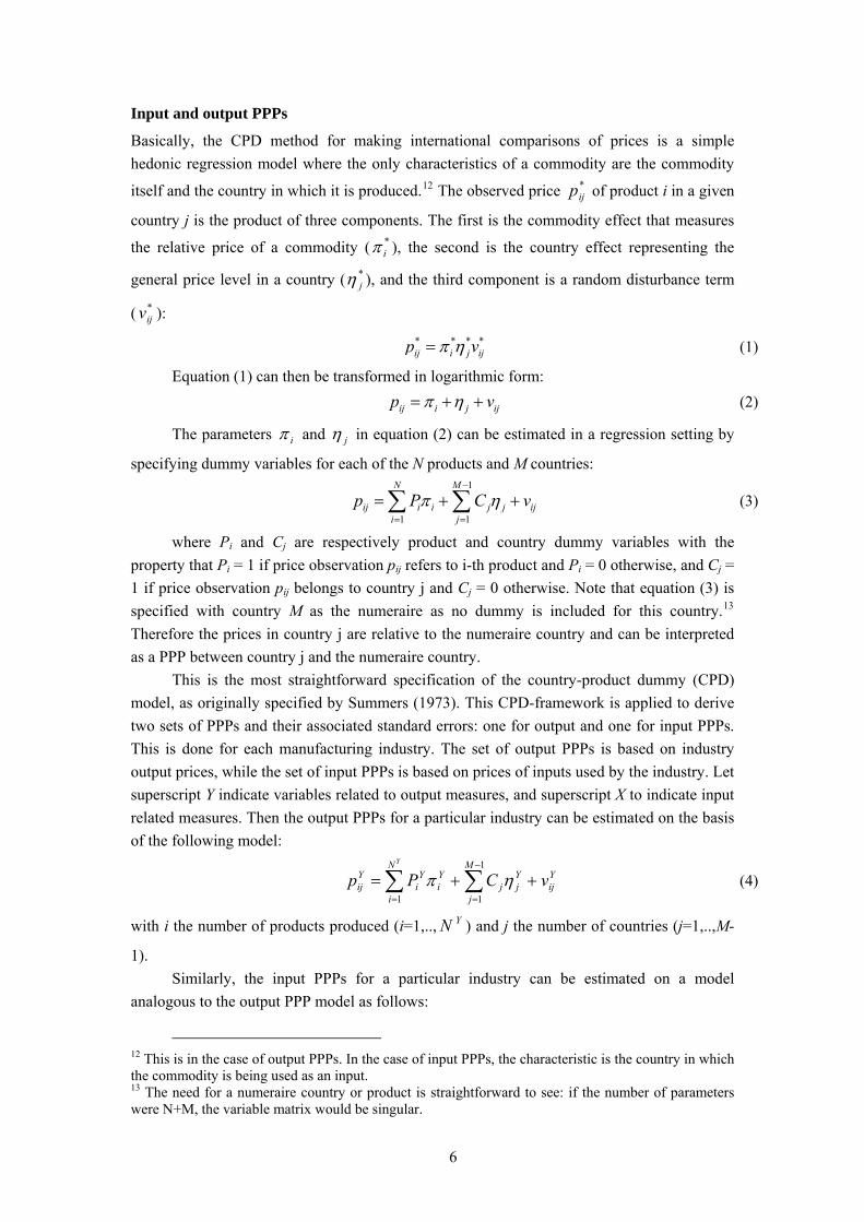
the output prices of a particular good in one country relative to another country and is based on a set of quantity and sales observations of more than 3,000 manufacturing goods. Input PPPs, which reflect the price of a particular input in one country relative to another, are based on a set of relative prices of 30 labor types, 8 capital asset types and 30 intermediate input types.

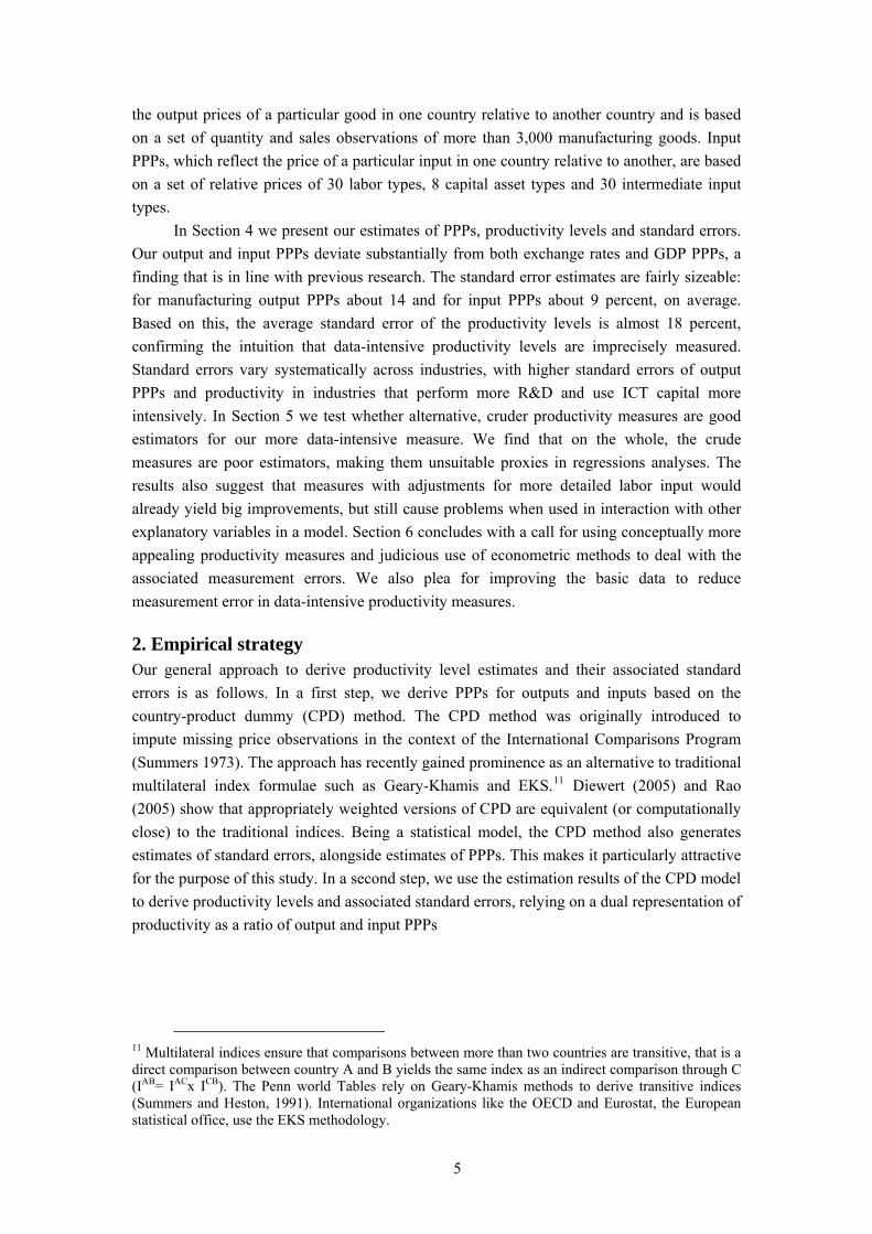
In Section 4 we present our estimates of PPPs, productivity levels and standard errors. Our output and input PPPs deviate substantially from both exchange rates and GDP PPPs, a finding that is in line with previous research. The standard error estimates are fairly sizeable: for manufacturing output PPPs about 14 and for input PPPs about 9 percent, on average. Based on this, the average standard error of the productivity levels is almost 18 percent, confirming the intuition that data-intensive productivity levels are imprecisely measured. Standard errors vary systematically across industries, with higher standard errors of output PPPs and productivity in industries that perform more R&D and use ICT capital more intensively. In Section 5 we test whether alternative, cruder productivity measures are good estimators for our more data-intensive measure. We find that on the whole, the crude measures are poor estimators, making them unsuitable proxies in regressions analyses. The results also suggest that measures with adjustments for more detailed labor input would already yield big improvements, but still cause problems when used in interaction with other explanatory variables in a model. Section 6 concludes with a call for using conceptually more appealing productivity measures and judicious use of econometric methods to deal with the associated measurement errors. We also plea for improving the basic data to reduce measurement error in data-intensive productivity measures.

2. Empirical strategy Our general approach to derive productivity level estimates and their associated standard errors is as follows. In a first step, we derive PPPs for outputs and inputs based on the country-product dummy (CPD) method. The CPD method was originally introduced to impute missing price observations in the context of the International Comparisons Program (Summers 1973). The approach has recently gained prominence as an alternative to traditional multilateral index formulae such as Geary-Khamis and EKS.11 Diewert (2005) and Rao (2005) show that appropriately weighted versions of CPD are equivalent (or computationally close) to the traditional indices. Being a statistical model, the CPD method also generates estimates of standard errors, alongside estimates of PPPs. This makes it particularly attractive for the purpose of this study. In a second step, we use the estimation results of the CPD model to derive productivity levels and associated standard errors, relying on a dual representation of productivity as a ratio of output and input PPPs

11 Multilateral indices ensure that comparisons between more than two countries are transitive, that is a direct comparison between country A and B yields the same index as an indirect comparison through C (IAB= IACx ICB). The Penn world Tables rely on Geary-Khamis methods to derive transitive indices (Summers and Heston, 1991). International organizations like the OECD and Eurostat, the European statistical office, use the EKS methodology.

5

Input and output PPPs

Basically, the CPD method for making international comparisons of prices is a simple hedonic regression model where the only characteristics of a commodity are the commodity

itself and the country in which it is produced.12 The observed price of product i in a given

country j is the product of three components. The first is the commodity effect that measures

the relative price of a commodity ( ), the second is the country effect representing the

general price level in a country ( ), and the third component is a random disturbance term

( ):

*ijp

*iπ

*jη

*ijv

* * *ij i j ij

*p vπ η= (1)

Equation (1) can then be transformed in logarithmic form: ij i j ijp vπ η= + + (2)

The parameters iπ and jη in equation (2) can be estimated in a regression setting by

specifying dummy variables for each of the N products and M countries:

1

1 1

N M

ij i i j j iji j

p P Cπ η−

= =

v= +∑ ∑ +

(3)

where Pi and Cj are respectively product and country dummy variables with the property that Pi = 1 if price observation pij refers to i-th product and Pi = 0 otherwise, and Cj = 1 if price observation pij belongs to country j and Cj = 0 otherwise. Note that equation (3) is specified with country M as the numeraire as no dummy is included for this country.13 Therefore the prices in country j are relative to the numeraire country and can be interpreted as a PPP between country j and the numeraire country.

This is the most straightforward specification of the country-product dummy (CPD) model, as originally specified by Summers (1973). This CPD-framework is applied to derive two sets of PPPs and their associated standard errors: one for output and one for input PPPs. This is done for each manufacturing industry. The set of output PPPs is based on industry output prices, while the set of input PPPs is based on prices of inputs used by the industry. Let superscript Y indicate variables related to output measures, and superscript X to indicate input related measures. Then the output PPPs for a particular industry can be estimated on the basis of the following model:

(4) Yij

M

j

Yjj

N

i

Yi

Yi

Yij vCPp

Y

++= ∑∑−

==

1

11ηπ

with i the number of products produced (i=1,.., ) and j the number of countries (j=1,..,M-

1).

YN

Similarly, the input PPPs for a particular industry can be estimated on a model analogous to the output PPP model as follows:

12 This is in the case of output PPPs. In the case of input PPPs, the characteristic is the country in which the commodity is being used as an input. 13 The need for a numeraire country or product is straightforward to see: if the number of parameters were N+M, the variable matrix would be singular.

6

(5) Xkj

M

j

Xjj

N

k

Xk

Xk

Xkj vCPp

X

++= ∑∑−

==

1

11ηπ

with k the number of inputs (k=1,.., ). XN

As argued by Rao (2005), a weighted version of the CPD is to be preferred in case output or input shares of the products are available, to ensure that more important products get a heavier weight in the index. This ensures that the resulting PPPs are close to those derived with traditional index number formulae. Following Rao (2005), we therefore pre-multiply the regression model given by equation (4) by the square root of the output weights as follows:

Yij

M

j

Yjj

Yij

N

i

Yi

Yi

Yij

Yij

Yij uCwPwpw

Y

++= ∑∑−

==

1

11

ηπ (6)

with the share of product i in total industry output in country j. These weights add up to 1

for each country. The input PPPs for a particular industry are estimated on a weighted CPD model analogous to the output PPP model as follows:

Yijw

Xkj

M

j

Xjj

Xkj

N

k

Xk

Xk

Xkj

Xkj

Xkj uCwPwpw

X

++= ∑∑−

==

1

11ηπ (7)

with the share of input k in total industry input cost in country j. Xkjw

We estimate the weighted CPD models by applying OLS to the transformed variables, using a tilde to indicate that a variable has been multiplied by its corresponding weight:

(8) Yij

M

j

Yjij

N

i

Yi

Yij

Yij uCPp

Y

++= ∑∑−

==

1

11

~~~ ηπ

(9) Xkj

M

j

Xjkj

N

k

Xk

Xkj

Xkj uCPp

X

++= ∑∑−

==

1

11

~~~ ηπ

The random disturbance terms and are assumed to be independently and

normally distributed with zero mean. The resulting estimates of η’s are used to obtain

estimates of input and output PPPs for each country using

Yiju X

kju

( )Yj

YjPPP η̂exp= and

( )Xj

XjPPP η̂exp=

Yj

Yj ses =)ˆ.(. η

. The estimated standard error of each ln(PPP) is given by respectively

and . Xj

Xj ses =)ˆ.(. η

The CPD model in equation (1) constitutes a purely statistical measurement model of cross-country price differences and is not predicated on any theory of price determination. As such the random component in the model can be interpreted as classical measurement error due to sampling, reporting and miscellaneous errors in prices. However, some models in international trade theory provide an interesting alternative interpretation: errors can also be seen as an indicator of the failure of arbitrage in international markets. Generally, manufacturing goods in the OECD are highly tradable and in a world governed by the Law of One Price, all manufacturing output prices in a country relative to foreign prices should be equal to the exchange rate. However, there is abundant evidence that shows that the law of

7

one price fails, particularly in the short run.14 Hence, part of the standard error in our model would not be measurement error but due to the many barriers to arbitrage. This is further discussed in Section 4. Similarly, distortions in labor and capital markets might (partly) be responsible for variation in wage and rental prices across countries. For example, it is well-known that in many European countries relative wages between high- and low-skilled workers are compressed compared to the U.S. due to more stringent labor legislation. So in practice, the disturbance terms of our models will also reflect such systematic factors and only partly consist of random errors. The standard error estimates should therefore be seen as upper bounds of the true measurement errors.15

Productivity levels

In measuring differences in productivity levels across countries, we follow a standard approach and define a Hicks-Moorsteen productivity index of country j relative to the US,

, as follows: jA

( )

( )j US

jj US

Y YA

X X= (10)

where Y and X are an output and input volume index respectively. Due to the nature of our data set, volume indices are indirectly defined through deflation and expressed as a ratio of the nominal value and a price index. As we use the ex-post approach to capital measurement (see data section) total input cost equals total output for each industry and it is easy to see that (10) can be written into its dual counterpart:

X

jj Y

j

PPPA

PPP= (11)

After taking logarithms, the relative productivity levels are then calculated from the coefficient estimates of equations (8) and (9) as the difference between the estimated input PPP and the output PPP.

ˆ ˆ ˆln X Yj jA jη η= − (12)

Nominal output is assume to be measured without error. In that case, the variance of the productivity level is given by

( ) ( ) ( ) ( )ˆ ˆ ˆ ˆvar ln var var 2cov ,Y X Y ˆ Xj j j jA jη η η= + − η

demand and prices. The productivity increase will also allow the industry to reduce output

(13)

where the variance of the input and output PPPs follow from estimating models (8) and (9). As we do not have an estimate of the covariance between input and output PPPs, we assume it is zero. This assumption likely overstates the standard error of productivity levels as there are good economic reasons why output and input prices would tend to vary positively together.

For example, if demand for an industry’s output increases, the industry will also require more inputs. As a result, both output and input prices will increase. Similarly, if an industry improves its productivity, it will require fewer inputs per unit of output, reducing input

14 See Goldberg and Knetter (1997) for a general overview, and Imbs et al. (2005) for evidence based on expenditure prices. 15 See also Deaton (2006) for this interpretation of errors in CPD-models.

8

prices relative to input prices. The strength of this covariance between input and output prices will depend on the particular structure of input and output markets, but the sign is presumably positive. In other words, the covariance in equation (13) will most likely be positive, or at least non-negative. The ‘true’ standard error of productivity levels will therefore be no larger than the estimate we arrive at by assuming zero covariance. Together with distortions in international product and factor markets discussed above, this is another reason why our results on standard errors of productivity levels should be seen as an upper bound of the true measurement error.

3. Data sources 12 manufacturing industries of 18 countries for the year 1997. The 12

93 manufacturing produ

Our database coversindustries cover the entire manufacturing sector (except oil refining) and with our 18 countries, we cover much of the OECD and European Union. Appendix Tables A1 and A2 provide full lists of respectively industries and countries included. The basis for the calculation of output PPPs is a large international product-level database containing quantity and sales observations of more than 3,000 manufacturing products. Input PPPs are based on relative prices of labor, capital and intermediate inputs following Jorgenson and Nishimizu (1978). Data on various types of labor and capital are derived from the EU KLEMS database (described in O’Mahony and Timmer, 2009). Intermediate input prices are based on corresponding output prices of the delivering industry. The main characteristics of the database are given in Table 1. Below, a more detailed description is given.

Our dataset for estimating output PPPs consists of a product list of 30cts containing data on the sales value and quantity sold. The basic data source for this

dataset is PRODCOM, which a harmonized set of product data for European Union member states (Eurostat, Prodcom database, 1997). The PRODCOM database is essentially based on the original national production censuses and industry surveys, but uses a harmonized product coding system. Since its start in the mid 1990s, PRODCOM’s coverage has greatly expanded, although there are still some gaps at 3-digit industry level (and also for 2-digit mineral and oil refining). The PRODCOM data for 1997 covers only the old EU-15 countries (Austria, Belgium, Denmark, Finland, France, West-Germany, Ireland, Italy, Netherlands, Portugal, Spain, Sweden and United Kingdom). We used national census and production survey data of other countries (Australia, Canada, Czech Republic, Hungary, Japan and the US) to enlarge the country coverage by linking each national product list with the PRODCOM classification. The classification of the products is by an 8-digit product code which allows for a narrow product description.16 For example the list contains the following products: Pig-meat: fresh or chilled: carcasses and half-carcasses (code 15111330) and Cold rolled narrow strip, width <= 500 mm, of non alloy steel, 0.25% >= C < 0.6% (code 27321031). The sales value is divided by the quantity sold to construct unit values which are used to proxy sales prices. The raw data has been cleaned for outliers. All unit values of a product that fell outside the range of 0.2 and 5 times the average across all countries were removed.17 Finally, the dataset was

16 This classification is the PRODCOM product classification of Eurostat, which is linked at the 4-digit level to the NACE (rev 1) industry classification. 17 This was applied recursively so the average reflects the average of the data that is in the cleaned dataset, not the original one.

9

complemented by a hedonic output PPP for automobiles. The end result of this merging was a list of 3,093 manufacturing products for which quantities and sales values were available for at least two countries. The database contains a sizeable number of missing values, and coverage differs by country and industry. On average we have about 1,044 observations per industry, ranging from a low 306 in transport equipment manufacturing to a high 2,340 in food and beverages manufacturing (see Appendix Table 1). In general, the EU countries have a higher coverage than the other countries. As shown in Appendix Table 2, the average number of observations in Hungary and Australia was less than 10 per industry, while more than 130 in Germany, Italy and Spain.

Unit values have been used as proxy for output, import and export prices in various other

side, we distinguish 60 types of inputs: 29 types of domestically produced interm

purchased at the prevailing US$ exchange rate (from IMF, Financial Statistics).20

studies, but are known to suffer from the so-called “quality problem”. Unit values can be considered as basic prices averaged over all producers and across a set of loosely specified products. They are often an average of a mix of products of varying degrees of homogeneity. In particular for industries producing sophisticated goods, such as machinery or electronic equipment, the product descriptions are not sufficient to capture all relevant characteristics of the goods. Consequently, a difference in unit values between two countries could be measuring not merely a difference in price, but also a difference in composition of product mix and difference in quality. Comparisons of unit values for automobiles are a notorious example and are an important manufacturing product in various countries. For this reason we relied on a hedonic study of automobile unit values which corrects for a range of important car characteristics (van Mulligen, 2003). Unfortunately, hedonic estimates are not available for all countries or for other products. Insofar as some countries produce lower quality varieties for a wide range of products, their PPPs will be underestimated and hence their productivity levels overestimated.18 This might be the case for less advanced countries like Hungary, Portugal and Spain, that invest much less in manufacturing R&D than the other countries in 1997.

On the input ediate inputs, total imported intermediates, 30 types of labor and 8 types of capital.

Business statistics surveys and productivity censuses provide little or no information on quantities and values of inputs so in this study we use output PPPs as a proxy for relative intermediate input prices under the assumption that the basic price of a good is independent of its use. That is, we use the same gross output PPP of an industry to deflate all intermediate deliveries from this industry to other industries, mimicking standard practice in National Accounts. These output PPPs are taken from Timmer, Ypma and van Ark (2007).19 The PPP for imported intermediates is taken as the exchange rate, assuming that all imports are

18 Unit values are used in tracking price change e.g. in Lichtenberg and Griliches (1989) and Siegel

r et al., 2007; Feenstra et al., 2009).

based on trade data as there is little

(1997). They have also been extensively used in cross-country price comparisons (van Ark and Pilat, 1993; Rao et al. 1995; Timme19 These output PPPs refer to basic prices, but as we include transportation and trade services as separate inputs, the total inputs are valued at purchaser prices (see Inklaar and Timmer, 2007). 20 Ideally, one would like to have separate estimates of import PPPsevidence that the law of one price holds for all goods even when internationally traded. However, so far this data is not readily available.

10

PPPs for labor inputs are derived by dividing a country’s wage rate by the corresponding US wage rate (Jorgenson and Nishimizu, 1978). This is done at a detailed level of agg

countries from Euros

ductivity levels and standard errors To derive manufacturing input and output PPPs, we estimated equations (8) and (9) with

cedure. Table 2 shows the resulting

rkets. One of the cornerstones in standard international trade theory i

where the price is high. This law is the foundation of the PPP hypothesis which states that the

regation as characteristics of workers vary greatly across countries. Labor input is cross-classified by type of education (5 types), age (3 types) and gender, into 30 groups. For each group in each industry, wages per hour worked are taken from the EU KLEMS database. They include all costs incurred by the producers in employment of labor. Capital PPPs give the relative price of the use of a unit of capital in two countries from the purchasers’ perspective. Under the assumption that the relative efficiency of new capital goods is the same in both countries, the relative rental price of a unit of capital between two countries depends on the relative investment price and the user cost of capital. The latter depends on the rate of return to capital, the depreciation rate and the investment price change. Following Jorgenson and Nishimizu (1978) we use the internal rate of return which ensures that capital rental prices times capital stocks equal total capital compensation. Capital PPPs are constructed for 8 groups of capital, including both ICT and non-ICT assets.21

The shares of each input in total input costs is derived from the EU KLEMS database, supplemented by national Supply and Use Tables (SUTs) of the varying

tat. The EU KLEMS data contains values of gross output, total intermediate input and groups of labor and capital. Total intermediate inputs from EU KLEMS are further subdivided into 30 groups based on national SUTs. This is done for each of the twelve manufacturing industries.22

4. PPPs, pro

OLS, adjusting for heteroscedasticity using White’s proPPPs for manufacturing output and inputs. Regressions have been run for each of the 12 industries separately, but a (value added) weighted average for total manufacturing is shown to save space.23 Columns 1 and 2 provide the relative price levels defined as the PPP divided by the exchange rate. Column 1 shows that exchange rates are generally not a good indicator of manufacturing output prices, as many values are far from one. In 1997, the exchange rate appeared to be highly overvalued in Czech Republic and Hungary, while undervalued in Ireland, Japan and the UK.

This variance might come as a surprise as most manufacturing products are highly tradable in international ma

s the Law of One Price: the price of an internationally traded good should be the same anywhere in the world once that price is expressed in a common currency. This law is based on an international goods arbitrage argument: in case prices of goods would differ, a riskless profit could be made by shipping them from countries where the price is low to countries

nominal exchange rate between two currencies should be equal to the ratio of aggregate price

21 See Inklaar and Timmer (2009) for more information. 22 In our definition of inputs we exclude own-industry deliveries, which corresponds to a definition of sectoral output. As a result our productivity measures are not dependent on the degree of vertical integration (see Gollop 1979 and Inklaar and Timmer, 2007). 23 Detailed results for each industry are given in Appendix Table A3.

11

levels between the two countries; hence the relative price level should be one. However, there are many reasons for the PPP hypothesis not to hold in the short run, including volatile exchange rate behavior and the many barriers to arbitrage which include tariff and non-tariff barriers, transport costs, product differentiation and price discrimination (Goldberg and Knetter, 1997; Anderson and van Wincoop, 2004). In general there is consensus that PPP should hold in the long run, but not necessarily in the short run (Taylor and Taylor, 2004). Based on a panel of detailed expenditure prices, Imbs et al. (2005) find that price differentials across countries can be very persistent also at lower levels of aggregation. In particular, they find that the degree of persistence is quite heterogeneous across sectors. Our results confirm these findings as output PPPs not only differ substantially from the exchange rate in most countries, but also differ widely across industries.24

As an alternative to using exchange rates as currency converters in productivity comparisons, most studies rely on the overall GDP PPP as given in the Penn World Tables (Summers and Heston, 1991). However, the correlation of the manufacturing output PPPs with overall GDP PPPs, given in the last column, is weak. GDP PPPs reflect prices of all goods a

ut PPPs differ widely from the exchange rates. In

utput PPPs ar

nd services in the economy and are mainly determined by relative prices of services. Typically, GDP PPPs are lower in countries with lower levels of GDP per capita due to the Harrod-Balassa-Samuelson effect stating that the relative price of tradables compared to non-tradables is higher in less productive countries. This effect is clearly visible for the lowest-income countries in our group as the manufacturing output PPP is much higher than the GDP PPP. This finding suggest that the use of GDP PPPs for comparing sectoral output in cross-country comparisons might be misleading and underlines the warnings issued by Sørenson (2001) not to use them in convergence analysis.25

Column 2 of Table 2 shows the ratios of input PPPs over the exchange rates. Estimates of sectoral input PPPs are scarce due to the high data requirements.26 Input PPPs reflect prices of all energy, material and services inputs used in an industry, together with labor and capital inputs. As for output PPPs, inp

contrast, the correlation of input PPPs with aggregate GDP PPPs is much higher than of output PPPs. This is particularly clear for less advanced countries such as Czech Republic, Hungary and Portugal. This positive correlation is to be expected. Typically, the inputs in an industry cover a wide range of goods and services which are sourced from all sectors in the economy. Also, many of these inputs are not specific to one industry, generating relatively little differences in the input PPPs across industries in a country.27

The main aim of this study is to estimate standard errors associated with the PPPs. These are then used to derive standard errors of MFP levels as outlined in Section 2. Table 3 gives the standard errors of output PPPs, input PPPs and MFP levels for each manufacturing industry as an unweighted average across our set of countries. The standard errors for o

e given in the first column and found to be substantial, on average 14%. In general errors for input PPPs are smaller, averaging at 9%. Based on equation (13) the standard errors

24 Detailed results for each industry are given in Appendix Table A3. 25 See Inklaar and Timmer (2009) for a discussion. 26 The seminal study is by Jorgenson, Kuroda and Nishimizu (1987). For recent applications, see Lee and Tang (2000) and Inklaar and Timmer (2009). 27 Detailed results for each industry are given in Appendix Table A3.

12

of the productivity levels have been derived and the results confirm the commonly held opinion that measurement error in data-intensive productivity measures is large. In some industries, the standard errors are higher than 20 percent. The errors for MFP are always larger than for output PPPs. This magnifying effect of errors is akin to the classical double deflation problem of value added which has been widely discussed in the past. Double-deflated value added volumes, calculated as the growth of output minus the weighted growth of intermediate inputs, appeared to be highly sensitive to measurement errors in either output or inputs (Sims, 1969). Only after price measurement in the National Accounts statistics had substantially improved, in particular for inputs, did double-deflated value added measures become standard practice in national statistical institutes. Similarly, given that productivity is calculated as the difference between input and output PPPs, a small percentage error in output or input PPPs appears as a much larger percentage error in productivity levels.

While the standard errors in Table 3 are substantial, we believe that our estimates are rather conservative and should be considered as upper bounds of the true measurement error as discussed in Section 2. First, there is abundant evidence that PPPs of individual inputs and outputs in an industry might differ due to imperfections in international and national product and fact

the variance in output P

or markets, particularly in the short run. As such, part of the measured variance is due to barriers to arbitrage in markets rather than to measurement error. Second, we assumed zero covariance between output and input PPPs while they are likely to be positively correlated. In that case, the magnifying error effect in MFP estimates would be less severe.

Given this, it is insightful to look also at the relative size of the standard errors as they vary widely across manufacturing industries. Table 3 shows that the standard error for MFP levels varies from a low 14% in the food and textile industries to over 23% in electrical and optical equipment industry. This variance across sectors is mainly due to

PPs and might be related to the quality problem of unit values which we use to proxy for output prices. As unit values are often based on a mix of products of varying degrees of homogeneity, PPPs could reflect not only a price difference, but also a difference in composition of product mix and difference in quality. Lichtenberg and Griliches (1989) and Siegel (1997) argue that the inability of unit values to capture quality differences has the largest consequences in industries that produce more sophisticated goods. Based on data for U.S. manufacturing industries, Lichtenberg and Griliches (1989) showed that output price indices based on unit values have a higher standard error than specified prices. This error was positively related to the R&D intensity of the industry as R&D is a major cause of product quality change and the introduction of new products. Siegel (1997) contends that more recently, investment in computers could also raise product quality by stimulating an increase in product innovation and development. In Table 3 we test these hypotheses in a cross-country setting by correlating measurement errors with R&D and ICT intensity across industries. The intensities are defined as R&D expenditure and ICT investment as a percentage of value added in 1997, averaged across our set of countries. The intensities are given in the last columns of Table 3. The correlations with the output PPPs in the bottom rows support the hypothesis that if firms in an industry spend more on innovation, new products will be introduced more rapidly and comparisons of products across countries will more likely be plagued by mismatches in product characteristics leading to higher standard errors. The correlation of the errors with ICT intensity is 41%, increasing to 60% in the case

13

of R&D intensity.28 Siegel (1997) also hypothesized that there might be a relationship between computer investment and the composition of the workforce. If there is complementarity between ICT and workers skills, and the latter is not sufficiently picked up by our comparisons of labor types across countries, standard errors of input PPPs might increase. This is not borne out by the simple correlation test. If anything a negative relationship is found, but it is insignificant.

5. Is more detailed data better? Our results so far have indicated that data-intensive estimates of cross-country MFP levels have substantial standard errors. This is due to the heavy requirements in terms of detailed data on output and input prices and quantities. Given these findings, for most applied

hether relatively crude measures which are less data

4)

e previous

ection. The latter is our closest approximation to the true proprodu eormeasure, the slope of the regression will be one and γ will be zero. If γ is significantly

l GDP deflat

researchers, the key question will be wdemanding might provide good approximations for the ‘true’ productivity levels. Under the assumption that our data-intensive productivity measure is an unbiased estimate of the true productivity level, we can test this directly by estimating the following regression:

ijCij

DIij AA εγα +−+= ln)1(ln (1

where CijA is a relatively crude measure of the productivity level of industry i in

country j while DIijA is the data-intensive productivity level we estimated in th

s ductivity levels in terms of ction th y concepts. If the crude measure is a good proxy for the data-intensive

different from zero though, we can reject the crude measure as a good proxy for the data-intensive measure as the bias in the crude measure is not constant across observations.

We will study four alternative MFP measures that have been used in the literature so far. The baseline measure is called the crude measure and follows the approach that has become standard practice in the literature starting with Bernard and Jones (1996). In this approach value added in each manufacturing industry is deflated by the same overal

or. Labor input is measured as number of workers which, in the dual representation of MFP is equivalent to using the overall wage rate as a PPP (calculated as overall labor compensation in an industry divided by the number of workers). Finally, capital input is measured as the real capital stock converted with the overall GDP PPP.29 We also look at various more refined measures that have been used so far. Griffith et al. (2004), Nicoletti and Scarpetta (2003) and Cameron et al. (2005) use additional data sources to adjust MFP for differences in average hours worked and for the composition of labor, distinguishing between

28 Correlation between R&D and ICT-intensity at the industry level is high and ICT intensity does not explain much beyond R&D alone. The correlations rely on the 12 data points given in the table, but a

re common primal formulation based on quantities.

regression explaining all country-industry data on standard errors (up to 204 observations) using average R&D intensities is highly significant and explains up to 14 percent of variation. The average R&D intensity is the appropriate concept since rapid innovation need not take place in each country for a mismatch in product qualities to occur. Lichtenberg and Griliches (1989) and Siegel (1997) also tested for R&D and ICT investment by an industry’s suppliers rather than the own industry. This appeared not to be significant. 29 As discussed in Section 2, as long as input costs exhaust output, the dual productivity measure based on prices is equivalent to the mo

14

production and non-production workers. Also, since the comment by Sørenson (2001), there is a greater awareness of the importance of correcting for output price differences across sectors and these studies have used sector-specific PPPs to convert value added. Compared to our preferred measure, price differences between outputs and the intermediate inputs are still ignored. Value added is defined as output minus intermediate inputs and implicitly it is assumed that PPPs of output and intermediate inputs in an industry are the same. Also, no adjustments are made for differences in marginal products between various types of capital assets.30

In Figure 1, we plot the four cruder (less data-intensive) MFP alternatives against our preferred measure. As both measures are expressed in logs, zero denotes a productivity level in an industry-country pair equal to that in the United States. The regression line corresponding to equation (14) is included in each plot and shows a positive relationship betwe

measure seems to provide a reasonable proxy for the data-intensive measu

n instead as follows:

5)

en the data-intensive measure and the cruder measures. A first observation is that the data-intensive measure tends to have a greater dispersion than the crude measures. This observation is consistent with the hypothesis that more data-intensive measures have greater measurement error. Moreover, with each refinement in the productivity measure, the dispersion increases.

The top part of Table 4 shows the regression results corresponding to the plots in Figure 1 for each of the four alternatives. They are based on an unweighted OLS regression as given in equation (14). The performance of the various alternative MFP measures is far from uniform. The crudest

re. As the point estimate of γ shows, the slope of the regression line is substantially different from one, but it is only significant at the 10% level. This might explain the common finding in the literature that refinements in the productivity measure often do not qualitatively change the results of the analysis. This is particularly true for studies that correct for hours worked and composition of the labor force (alternative 2). We could not find a significant difference between the data-intensive measure and this alternative, although there appears to be an important constant bias as indicated by the significant deviation of α from zero: alternative 2 consistently underestimates MFP levels relative to the US. Perhaps surprisingly, adjustments for sectoral output PPPs lead to worse MFP proxies. The slope coefficients for alternatives 3 and 4 are both significantly different from one.

However, parameter estimates in unweighted OLS might be biased as we found in the previous section that standard errors of the MFP levels differ across the country-industry observations so the degree of measurement error is not constant. We can therefore improve the estimation of equation (14) by estimating a weighted versio

ijCijij

DIijij AWAW εγα +−+= ln)1(ln (1

where the weights are given by the inverse of the standard errors of the data-intensive

productivity levels in industry i and country j : ( )DIijij AW lnvar1= . These standard errors

were derived in the previous section. The results of the weighted regression strengthen the results of the unweighted one. Alternatives with output PPP corrections perform still weakly.

30 For more details and discussion of these measures and differences between them, see Inklaar, Timmer and van Ark (2008) and Inklaar and Timmer (2009).

15

Now the slope estimate of the crude measure is also significantly one-pproductivi

bles. However, most recent applications in the popular “distance to the fro

d differences in marginal product between various types of labor and capital (such as skilled labor and ICT capital). While this has long been known from

chers have had to use cruder estimates due to a lack of suitable

different from one at the ercent significance level. This measure, which would make the poorest proxy for true

ty levels according to economic theory, has the slope estimate that is clearly the farthest away from one.31

Based on these results one can argue that the alternative with adjustments for labor appears to be the most reasonable proxy for the data-intensive measure. However, the significant bias in levels, as indicated by coefficient α, argues for caution in using this alternative in particular applications. The constant difference between measured and true MFP levels does not pose major difficulties in regression models without interactions between MFP levels and other varia

ntier”-models rely on interaction terms of the initial MFP level and variables that are assumed to facilitate or hinder the diffusion of frontier knowledge such as international trade, R&D effort, skills or product market regulation.32 In the Appendix we show that in those interaction models, a significant α-coefficient will cause a bias in the estimated marginal effect of the variable of interest.

6. Concluding Remarks In this paper we argue that the use of crude measures of MFP levels in studies of economic growth and international trade might be misleading. Production theory implies that estimates of industry productivity levels should take account of many factors: differences in input and output prices across countries an

a theoretical perspective, researdata. With the increasing availability of the right type of data though, estimating conceptually preferred productivity levels has become feasible. The main contribution of this paper is to propose and implement a coherent framework to estimate both productivity levels and corresponding standard errors. This framework is based on country-product dummy (CPD) regressions and data on relative input and output prices in 12 manufacturing industries across 18 OECD countries. Using this framework, we show that the standard errors in productivity levels are sizeable, but also that they differ considerably across industries and countries. We have also shown that the crude measures often used in the literature are not a good proxy for measures that are conceptually superior. Even MFP measures which are adjusted for hours worked and skill composition of the labor force are not adequate in regression models in which the MFP level is interacted with other variables. Instead, these models should use data-intensive measures that also adjust for prices of intermediate inputs and various capital assets. These measures are based on more detailed data and, because of that, more sensitive to measurement error.

Knowledge of the standard error of MFP levels is potentially useful in at least two respects. First, these estimates might be useful in estimating consistent parameters in

31 In terms of Figures 1, some of the influential observations appeared to be also observations with relatively high standard errors so these observations were given a lower weight in the weighted regression. Crucially though, this weighting was done because of high standard errors, not because these observations were outliers. 32 See footnote 2 for examples.

16

econometric models that include error-ridden MFP levels on the right-hand side. In this case, standard estimation using ordinary least squares (OLS) will lead to biased and inconsistent estimates of both the coefficient and standard errors. This is a familiar problem, but so far has only be studied in cases where the degree of measurement error is unknown (Temple, 1998). More

, 2001) are also prevalent in compari

recently, Wansbeek and Meijer (2000) showed how to adjust OLS parameters and standard errors when measurement error is known. Estimates of measurement error in MFP levels could be used in applications of their proposed consistently adjusted least squares (CALS) estimator. Our finding of differences in measurement error across industries and countries might require additional adjustments to this technique.

The second respect in which these estimates might be useful is in indicating areas of improvement in statistical data. We would like to stress that our estimates of MFP levels and their associated standard errors are still experimental. They are based on a wide variety of official data sources from national statistical institutes, whose reliability differs and consistency is far from perfect. Difficulties in measuring productivity growth rates within a country based on the present system of national accounts (Diewert

sons of MFP levels between countries. Sometimes, they are even more severe, such as in comparisons of levels of educational attainment (O’Mahony and Timmer, 2009). A major challenge in reducing measurement error lies in accounting for differences in the quality of goods produced. We have shown that the degree to which an industry spends on innovation is a good predictor of the standard error of its output PPP. This suggests a more in-depth focus on output prices of products from high-tech industries such as electronics and machinery. This would also improve PPPs for capital assets. Piecemeal progress on this is being made both within statistical agencies and in the academic world, for example through using hedonic techniques. Since the CPD framework used in this study is a very simple hedonic model, it can serve as a basis for relative price estimates that better take into account quality differences. Recent work also suggests that detailed barcode scanner data can be used to compare product prices across countries at a very detailed level, drastically reducing the problem of quality differences.33 So far, studies have mainly focused on improving relative price measures for manufacturing products and increasing attention is needed for comparisons of prices of services given their rising importance in production. In general though, we have shown in this paper that there are important gains from using detailed data, giving us hope that further improvements will pave the way to sharper, more comprehensive studies of economic growth and international trade.

33 See e.g. Goldberg and Verboven (2001) and Heravi, Heston and Silver (2003) for an application of hedonics. The latter study is based on scanner data. See also Broda and Weinstein (2008).

17

References Acemoglu, Daron and Fabrizio Zilibotti, “Productivity Differences” Quarterly Journal of

Economics, 116:2 (2001), 563-606. Acemoglu, Daron, Philippe Aghion and Fabrizio Zilibotti, “Distance to Frontier, Selection,

and Economic Growth” Journal of the European Economic Association 4:1 (2006), 37-74

Aghion, Philippe and Peter W. Howitt, The Economics of Growth, (Cambridge, MA: MIT Press 2009).

Anderson, James E. and Eric van Wincoop, “Trade Costs,” Journal of Economic Literature, 42:3 (2004), 691-751.

Baumol, William J., “Productivity Growth, Convergence, and Welfare: What the Long-Run Data Show” American Economic Review, 76:5 (1986), 1072-1085.

Bernard Andrew B. and Charles I. Jones, “Comparing Apples to Oranges: Productivity Convergence and Measurement Across Industries and Countries,” American Economic Review 86:5 (1996), 1216-1238.

Bernard Andrew B. and Charles I. Jones, “Comparing Apples to Oranges: Productivity Convergence and Measurement Across Industries and Countries: Reply,” American Economic Review 91:4 (2001), 1168-1169.

Brambor, Thomas, William R. Clark and Matt Golder, “Understanding Interaction Models: Improving Empirical Analyses” Political Analysis, 14:1 (2006), 63-82.

Broda, Christian M. and David E. Weinstein, “Understanding International Price Differences using Barcode Data,” NBER Working Paper no. 14017 (2008).

Cameron, Gavin, James Proudman and Stephen Redding, “Technological Convergence, R&D, Trade and Productivity Growth,” European Economic Review, 49 (2005), 775-807.

Caselli, Francesco and Daniel J. Wilson, “Importing technology,” Journal of Monetary Economics 51:1 (2004), 1-32.

Caselli, Francesco, “Accounting for Cross-Country Income Differences” in Philippe Aghion and Steven N. Durlauf (Eds.), Handbook of Economic Growth (Elsevier 2005), 679-741.

Cohen, Daniel and Marcelo Soto, “Growth and human capital: good data, good results,” Journal of Economic Growth, 12:1 (2007), 51-76.

Deaton, Angus, “Purchasing Power Parity exchange rates for the poor: using household surveys to construct PPPs” mimeo, Princeton University (2006).

de la Fuente, Angel and Rafael Doménech, “Human capital in growth regressions: how much difference does data quality make?” Journal of the European Economic Association, 4:1 (2006), 1-36.

De Long, J. Bradford, “Productivity Growth, Convergence, and Welfare: Comment” American Economic Review, 78:5 (1988), 1138-1154.

Diewert, W. Erwin, “Which (Old) Ideas on Productivity Measurement Are Ready To Use?” in Charles R. Hulten, Edwin Dean and Michael J. Harper (Eds.) New Developments in Productivity Analysis (Chicago: University of Chicago Press, 2001), 85-102.

Diewert, W. Erwin, “Weighted Country Product Dummy Variable Regressions and Index

18

Number Formulae,” Review of Income and Wealth 51:4 2005, 561-570. Durlauf, Steven N., Paul A. Johnson and Jonathan R.W. Temple, “Growth Econometrics” in

Philippe Aghion and Steven N. Durlauf (Eds.) Handbook of Economic Growth (Elsevier 2005), 555-677.

Feenstra, Robert C., Alan Heston, Marcel P. Timmer and Haiyan Deng, “Estimating Real Production and Expenditures across Nations: A Proposal for Improving the Penn World Tables,” Review of Economics and Statistics 91:1 (2009), 201-212.

Ghironi, Fabio and Marc J. Melitz, “International Trade and Macroeconomic Dynamics with Heterogeneous Firms,” Quarterly Journal of Economics 120:3 (2005), 865-915.

Goldberg Pinelopi K. and Verboven, “The Evolution of Price Dispersion in the European Car Market,” Review of Economic Studies, 68:4 (2001), 811-848.

Goldberg, Pinelopi K. and Michael M. Knetter, “Goods Prices and Exchange Rates: What Have We Learned?” Journal of Economic Literature, 35:3 (1997), 1243-1272.

Gollop, Frank M., “Accounting for intermediate input: the link between sectoral and aggregate measures of productivity,” in Measurement and Interpretation of Productivity (Washington, DC: National Academy of Sciences, 1979), 318-333.

Griffith, Rachel, Stephen J. Redding and John Van Reenen “Mapping the two faces of R&D: productivity growth in a panel of OECD industries,” Review of Economics and Statistics, 86:4 (2004), 883-895.

Griliches, Zvi, “Economic data issues,” in: Zvi Griliches and Michael D. Intriligator (Eds.), Handbook of Econometrics volume 3, (Elsevier, 1986), 1465-1514.

Harrigan, James, “Technology, Factor Supplies, and International Specialization: Estimating the Neoclassical Model,” American Economic Review, 87:4 (1997), 475-494.

Heravi, Saeed, Alan Heston and Mick Silver, "Using Scanner Data to Estimate Country Price Parities: A Hedonic Regression Approach," Review of Income and Wealth, 49:1 (2003), 1-21.

Hsieh, Chang-Tai and Peter J. Klenow, “Relative Prices and Relative Prosperity,” American Economic Review, 97:3 (2007), 562-585.

Imbs, Jean, Haroon Mumtaz, Morten O. Ravn, Hélène Rey, “PPP Strikes Back: Aggregation and the Real Exchange Rate,” Quarterly Journal of Economics, 120:1 (2005), 1-43.

Inklaar, Robert and Marcel P. Timmer, “International Comparisons of Industry Output, Inputs and Productivity Levels: Methodology and New Results,” Economic Systems Research, 19:3 (2007), 343-364.

Inklaar, Robert and Marcel P. Timmer, “Productivity Convergence Across Industries and Countries: The Importance of Theory-based Measurement,” forthcoming in Macroeconomic Dynamics, (2009).

Inklaar, Robert, Marcel P. Timmer and Bart van Ark, “Market services productivity across Europe and the US,” Economic Policy, 23:53 (2008), 139-194.

Islam, Nazrul, “What have we learnt from the convergence debate?” Journal of Economic Surveys, 17:3 (2003), 309-362.

Jorgenson, Dale W. and Khuong Vu, “Information Technology and the World Economy,” Scandinavian Journal of Economics, 107:4 (2005), 631-650.

Jorgenson, Dale W. and Mieko Nishmizu “U.S. and Japanese economic growth, 1952-1974: an international comparison,” Economic Journal, 88 (1978), 707-726.

19

Jorgenson, Dale W. Productivity: International Comparisons of Economic Growth (Cambridge MA: MIT Press, 1995).

Jorgenson, Dale W., Masahiro Kuroda and Mieko Nishimizu, “Japan-U.S. industry-level productivity comparisons, 1960-1979,” Journal of the Japanese and International Economies, 1 (1987), 1-30.

Keller, Wolfgang, “Trade and the Transmission of Technology,” Journal of Economic Growth, 7:1 (2002), 5-24.

Klepper, Steven and Edward E. Leamer, “Consistent Sets of Estimates for Regressions with Error in all Variables” Econometrica, 52:1 (1984), 163-183.

Lee, Frank and Jianmin Tang, “Productivity Levels and International Competitiveness between Canadian and U.S. Industries”, American Economic Review, 90:2 (2000), 176-79.

Lichtenberg, Frank R. and Zvi Griliches, “Errors of Measurement in Output Deflators” Journal of Business & Economic Statistics, 7:1 (1989), 1-9.

Nicoletti, Giuseppe and Stefano Scarpetta, “Regulation, Productivity and Growth: OECD Evidence,” Economic Policy, 36:1 (2003), 9-72.

O’Mahony, Mary and Marcel P. Timmer, “Output, Input and Productivity Measures at the Industry Level: the EU KLEMS Database,” forthcoming in Economic Journal (2009).

Rao, D.S. Prasada, E. Anthony Selvanathan and Dirk Pilat, “Generalized Theil-Tornqvist Indices with Applications to International Comparisons of Prices and Real Output” Review of Economics and Statistics, 77:2 (1995), 352-60,

Rao, D.S. Prasada, “On the Equivalence of Weighted Country-Product-Dummy (CPD) Method and the Rao-System for Multilateral Price Comparisons” Review of Income and Wealth, 51:4 (2005), 571-580.

Rogerson, Richard, “Structural Transformation and the Deterioration of European Labor Market Outcomes,” Journal of Political Economy, 116:2 (2008), 235-259.

Siegel, Donald, “The Impact of Computers on Manufacturing Productivity Growth: A Multiple-Indicators, Multiple-Causes Approach” Review of Economics and Statistics, 79:1 (1997), 68-78.

Silver, Mick and Saeed Heravi, “The Measurement of Quality-Adjusted Price Changes” in Robert C. Feenstra and Matthew D. Shapiro (Eds.) Scanner Data and Price Indexes (Chicago: University of Chicago Press, 2003), 277-316.

Sims, Christopher A., “Theoretical Basis for Double Deflated Index of Real Value Added” Review of Economics and Statistics, 51:4 (1969), 470-471.

Sørensen, Anders “Comparing Apples to Oranges: Productivity Convergence and Measurement Across Industries and Countries: Comment,” American Economic Review 91:4 (2001), 1160-1167.

Summers, Robert, “International Comparisons with Incomplete Data,” Review of Income and Wealth, 29:1 (1973), 1-16.

Summers, Robert and Alan Heston, “The Penn World Table (Mark 5): An Expanded Set of International Comparisons, 1950-1988,” Quarterly Journal of Economics, 106:2 (1991), 327-368.

Taylor, M. P., and A. M. Taylor. “The Purchasing Power Parity Debate.” Journal of Economic Perspectives 8:4 (Fall 2004), 135–158.

20

Temple, Jonathan, “Robustness tests of the augmented Solow model,” Journal of Applied Econometrics, 13:4 (1998), 361-375.

Timmer, Marcel P. and Bart van Ark, “Does Information And Communication Technology Drive Productivity Growth Differentials? A Comparison Of The European Union Countries And The United States,” Oxford Economic Papers, 57:4 (2005), 693-716.

Timmer, Marcel P., Gerard Ypma, and Bart van Ark, “PPPs for industry output: a new dataset for international comparisons” GGDC Research Memorandum GD-82, Groningen: Groningen Growth and Development Centre (2007).

van Ark, Bart, and Dirk Pilat, “Productivity Levels In Germany, Japan And The United States,” Brookings Papers on Economic Activity, Microeconomics, 2 (1993), 1-48.

van Mulligen, Peter Hein, Quality aspects in price indices and international comparisons: Applications of the hedonic method, (Voorburg: Statistics Netherlands 2003).

Vandenbussche, Jérôme, Philippe Aghion and Costas Meghir, “Growth, Distance to the Frontier and Composition of Human Capital,” Journal of Economic Growth, 11:2 (2006), 97-127.

Wansbeek, Tom and Erik Meijer, Measurement Error and Latent Variables in Econometrics (Amsterdam: North Holland, 2000).

21

Table 1, Data sources Major type Description Data sourceA: Output prices Factory-gate unit values for a maximum of

3093 products across 12 industriesPRODCOM database for EU-15 countries. Manufacturing Censuses for other countries.

B: Output weights Product shares in total sales as A.

C: Input pricesIntermediate inputs (domestically produced)

Output PPPs for 29 domestic industries Based on Timmer, Ypma and van Ark (2006)

Imported intermediates Exchange rate IMF International Financial StatisticsLabour Relative wage for 30 types of workers (age x

gender x education)EU KLEMS

Capital EU KLEMS

D: Input weights Shares of inputs in total costs Eurostat Input-output tables and EU KLEMS

Relative rental prices for 8 types of capital based on investment PPPs and relative user costs of capital (using internal rates of return)

Table 2, Relative output and input prices in manufacturing and the relative price of GDP, 1997

Output PPP

Input PPP

GDP PPP

Australia 1.12 0.95 0.98Austria 1.22 1.11 1.04Belgium 0.93 1.07 1.03Czech republic 0.61 0.49 0.40Denmark 1.13 1.17 1.28Spain 0.80 0.87 0.82Finland 1.11 1.09 1.14France 1.07 1.11 1.09Germany 1.12 1.14 1.12Hungary 0.70 0.51 0.45Ireland 1.44 1.41 1.02Italy 0.80 0.91 0.93Japan 1.38 1.36 1.39Netherlands 1.10 1.02 1.03Portugal 0.92 0.78 0.77Sweden 1.13 1.13 1.22United Kingdom 1.55 1.06 1.04United States 1.00 1.00 1.00

Note: PPPs have been divided by the exchange rate. For each country a value-added weighted average across twelve manufacturing industries is given. Source: Authors’ calculations. GDP PPPs and exchange rates from OECD, Main Indicators.

22

Table 3, Standard errors of manufacturing output and input PPPs, 1997

Output PPP Input PPP ProductivityFood, beverages and tobacco 7.1% 11.8% 14.2% 0.3 1.8Textiles, wearing apparel and leather products 9.8% 9.2% 13.9% 0.4 1.3Wood and wood products 18.5% 10.8% 21.6% 0.2 1.0Paper, printing and publishing 11.8% 9.5% 16.0% 0.3 3.1Chemical products excluding pharmaceuticals 11.6% 10.5% 16.7% 2.2 1.9Rubber and plastics 12.7% 8.2% 15.4% 1.0 1.4Non-metallic mineral products 12.5% 10.8% 16.7% 0.7 1.5Basic metals and fabricated metal products 15.2% 8.1% 17.5% 0.7 1.7Machinery 15.8% 7.7% 17.9% 2.0 2.2Electrical and optical equipment 21.1% 9.4% 23.7% 5.7 3.9Transport equipment 19.2% 6.8% 20.6% 3.4 2.7Other manufacturing, incl. recycling 17.4% 7.7% 19.3% 0.4 1.8

Average 14.4% 9.2% 17.8% 1.4 2.0

Correlation with R&D intensity 0.60 -0.25 0.65Correlation with ICT intensity 0.41 -0.23 0.47

Standard errors R&D intensity

ICT intensity

Note: for each industry an unweighted average across 17 countries is given. R&D and ICT intensity is defined as business enterprise research and development expenditure and ICT investment respectively in 1997 divided by industry output Source: Authors’ calculations. R&D from OECD and ICT from EU KLEMS database (March 2008), see O’Mahony and Timmer (2009).

23

Table 4, Regression explaining data-intensive productivity levels using various alternatives

1 Crude measure 0.00 (0.03) 0.43 * (0.22)2 Labour PPP adjustment -0.05 *** (0.02) 0.16 (0.21)3 Output PPP adjustment 0.12 *** (0.01) -0.40 *** (0.07)4 Output PPP & labour PPP adj. -0.01 (0.01) -0.38 *** (0.07)

1 Crude measure -0.28 (0.24) 0.84 *** (0.28)2 Labour PPP adjustment -0.36 *** (0.13) 0.34 (0.27)3 Output PPP adjustment 0.88 *** (0.07) -0.70 *** (0.08)4 Output PPP & labour PPP adj. -0.17 ** (0.07) -0.55 *** (0.07)

Alternative

Alternative

Constant (α ) 1-slope (γ )A. Unweighted OLS

B. Weighted OLS

Notes: *, **, *** denote a coefficient significantly different from zero at the 10%, 5% and 1% level respectively. Regressions in panel A are based on unweighted OLS as in equation (14). Regressions in panel B are based on weighted OLS as in equation (15), using standard errors of MFP estimates as weights. The coefficient γ is one minus the slope of the regression of data-intensive measures on alternative measures. Heteroscedasticity consistent coefficient standard errors are in parentheses. Each regression is based on 198 observations. The following PPPs are used in the different alternative productivity measures: Alternative 1: Wage per person for labor, GDP PPP for other variables; Alternative 2: Wage per hour for each type of labor, GDP PPP for other variables; Alternative 3: Wage per person for labor, output PPP for value added, GDP PPP for other variables; Alternative 4: Wage per hour for each type of labor, output PPP for value added, GDP PPP for other variables.

24

Figure 1 Data-intensive versus alternative estimates of log productivity levels (US=0), unweighted regressions. Figure 1a Alternative 1

-1.0

-0.8

-0.6

-0.4

-0.2

0.0

0.2

0.4

0.6

0.8

-1.0 -0.8 -0.6 -0.4 -0.2 0.0 0.2 0.4 0.6 0.8

log

of p

rodu

ctiv

ity le

vels

(U.S

.=0)

, da

ta-in

tens

ive

mea

sure

log of productivity levels (U.S.=0), alternative 1 Figure 1b Alternative 2

-1.0

-0.8

-0.6

-0.4

-0.2

0.0

0.2

0.4

0.6

0.8

-1.0 -0.8 -0.6 -0.4 -0.2 0.0 0.2 0.4 0.6 0.8

log

of p

rodu

ctiv

ity le

vels

(U.S

.=0)

,da

ta-in

tens

ive

mea

sure

log of productivity level (U.S.=0), alternative 2

25

Figure 1c Alternative 3

-1.0

-0.8

-0.6

-0.4

-0.2

0.0

0.2

0.4

0.6

0.8

-1.0 -0.8 -0.6 -0.4 -0.2 0.0 0.2 0.4 0.6 0.8

log

of p

rodu

ctiv

ity le

vels

(U.S

.=0)

, da

ta-in

tens

ive

mea

sure

log of productivity level (U.S.=0), alternative 3 Figure 1d Alternative 4

-1.0

-0.8

-0.6

-0.4

-0.2

0.0

0.2

0.4

0.6

0.8

-1.0 -0.8 -0.6 -0.4 -0.2 0.0 0.2 0.4 0.6 0.8

log

of p

rodu

ctiv

ity le

vels

(U.S

.=0)

, da

ta-in

tens

ive

mea

sure

log of productivity level (U.S.=0), alternative 4 Notes: For a description of the various alternatives, see Table 4.

26

Appendix - Crude productivity measures and biased regression coefficients In the main text we analyzed whether crude productivity measures are good proxies for the conceptually preferable data-intensive measures. This will in part depend on the particular use of MFP level estimates in cross-country growth models. In this appendix we consider two archetypal models: convergence models in which MFP levels are used as explanatory variable in isolation, and so-called distance–to-the-frontier models in which MFP levels are interacted with other explanatory variables. We show under what conditions the use of crude productivity measures will lead to biased parameter estimates. Rewriting equation (14) to explicitly recognize that productivity levels are measured relative to another country, we get:

1,

, ,

ln ln( )

ln ln

DI Cij X ij X

ijDI Cij F ij F

A AA A

,α γ ε= + − + (A1)

We specify the productivity level in country X relative to the country with the highest productivity level in that industry, country F. If both α and γ are not significantly different

from zero, the crude measure ,ln lnCij X ij FA A ,

C can be used as a proxy for the data-intensive

measure in regression analysis. As we saw in Table 4 though, α and γ do differ significantly from zero for all alternative, cruder measures, so it is useful to explore in which situations

regression results will be biased if ,ln lnCij X ij FA A ,

C is used as an explanatory variable.

The standard model of convergence is given e.g. by Bernard and Jones (1996) who studied whether countries with lower relative productivity levels in an initial period showed faster subsequent growth:

1

,,

,

lnln

ln

DIij X

ijt X ijtDIij F t

AA

Aφ β

−

⎛ ⎞Δ = + +⎜ ⎟⎜ ⎟

⎝ ⎠η (A2)

Where t-1 denotes the initial period and t subsequent growth in a particular period. The variable of interest in equation (A2) is β: if this coefficient is significantly negative, the convergence hypothesis is supported.34 If a crude productivity measure is used instead of a data-intensive measure, we get the following expression from substituting (A2) in (A1) and rearranging:

( ) 1

1

1 ,,

,

lnln ( )

ln

Cij X

ijt X ijt ijtCij F t

AA

Aφ βα β γ βε η−

−

⎛ ⎞Δ = + + − + +⎜ ⎟⎜ ⎟

⎝ ⎠ (A3)

This expression shows that to get an unbiased estimate of β, γ needs to be zero. In the main text, we showed that for crude measures adjusted for labor input (alternative 3), γ is zero.

However, this is no longer true once models with an interaction term are estimated, as in distance–to-the-frontier models. In general, these models have the following form:

1

1 1

, ,,

, ,

ln lnln

ln ln

DI DIij X ij X

ijt X t t ijtDI DIij F ij Ft t

A AA Z

A A 1Zφ β δ φ−

− −

⎛ ⎞ ⎛ ⎞Δ = + + + +⎜ ⎟ ⎜ ⎟⎜ ⎟ ⎜ ⎟

⎝ ⎠ ⎝ ⎠η−

(A4)

34 Technically, it only supports the hypothesis of mean reversion, not convergence, see Islam (2003).

27

So, for example, in Griffith et al. (2004) the conditioning Z variable is R&D intensity. Other variables that have been used include openness to international trade, level of human capital and degree of product market regulation.35 Equation (A4) allows for the effect of the Z variable on productivity growth to differ depending on the distance to the frontier. Griffith et al. (2004) find that higher R&D intensity always has a positive effect on productivity growth, but that this effect is larger for industries that are farther away from the productivity frontier. In this type of models both α and γ need to be zero to get unbiased estimates of the marginal effects of the explanatory variables on MFP growth. Substituting equation (A1) into (A4) and taking derivates gives the following expressions for the marginal effects:

( ) ( ) ( ) 1

1

1 1,

, ,

ln

ln lnijt X

tC Cij X ij F t

AZ

A Aβ γ φ γ −

−

∂= − + −

∂ (A5)

( )1 1

1,

,

ln lnln

Cijt X ij X

Ct i t

A AZ A

δ φ α γ− −

,

j F

⎡ ⎤⎛ ⎞∂⎢ ⎥= + + − ⎜ ⎟⎜ ⎟∂ ⎢ ⎥⎝ ⎠⎣ ⎦

(A6)

Equation (A5) shows that the estimate of the marginal effect of the distance-to-the-frontier on productivity growth is only affected if γ is significantly different from zero. However, the marginal effect of Z on productivity growth is affected by both the α and γ coefficient as shown in (A6). We conclude that when estimating a model without interactions as in equation (A2), the only relevant concern is whether the chosen productivity level measure differs systematically from the data-intensive measure (γ ≠ 0). However, if an interaction term is included in the model as in equation (A4), a significant difference in the average level (α ≠ 0) will be problematic too since it affects the marginal effect of the variable of interest, Z.

35 See footnote 2 of main text.

28

Appendix table A1, List of industries, industry codes and number of output price observations (average per country) Industry NACE # of observationsFood, beverages and tobacco 15t16 130Textiles, wearing apparel and leather products 17t19 114Wood and wood products 20 22Paper, printing and publishing 21t22 31Chemical products excluding pharmaceuticals 24ex244 80Rubber and plastics 25 22Non-metallic mineral products 26 38Basic metals and fabricated metal products 27t28 67Machinery 29 87Electrical and optical equipment 30t33 56Transport equipment 34t35 17Manufacturing, nec; recycling 36t37 31

Appendix table A2, List of countries, acronyms and number of output price observations (average per industry) Country Acronym # of observationsAustralia AUS 9Austria AUT 46Belgium BEL 35Czech republic CZE 18Denmark DNK 72Spain ESP 132Finland FIN 36France FRA 84Germany GER 162Hungary HUN 7Ireland IRL 25Italy ITA 133Japan JPN 11Netherlands NLD 33Portugal PRT 70Sweden SWE 27United Kingdom UK 114United States US 32

29

Table A3 Relative output and input prices, manufacturing industries AUS AUT BEL CZE DNK ESP FIN FRA GER HUN IRL ITA JPN NLD PRT SWE UK US

Output PPPs15t16 0.94 1.14 0.95 0.58 1.07 0.91 1.16 1.17 1.02 0.47 1.18 1.03 2.17 0.96 1.06 1.18 1.84 1.0017t19 1.42 1.98 0.92 0.81 1.31 0.93 1.70 1.58 1.66 0.91 1.23 0.70 1.38 1.45 0.98 1.75 2.00 1.0020 1.16 1.99 1.70 0.53 1.57 0.94 1.35 1.19 1.51 0.54 1.84 1.05 2.86 1.46 1.00 1.36 2.39 1.0021t22 0.77 0.87 0.78 0.69 0.82 0.79 0.77 0.97 0.94 0.52 1.23 0.81 1.34 0.96 0.82 0.90 1.11 1.0024ex244 1.68 1.12 0.85 0.47 1.09 0.79 0.92 1.05 1.06 0.49 1.88 0.86 1.29 0.89 0.95 0.98 1.58 1.0025 n.a. 1.35 1.02 0.64 1.06 0.98 1.54 1.31 1.51 0.68 0.96 0.91 1.00 1.23 0.74 1.71 1.64 1.0026 0.89 0.88 0.68 0.48 0.90 0.54 0.81 0.86 0.83 0.39 0.86 0.58 0.88 0.89 0.59 1.05 1.28 1.0027t28 0.99 1.48 1.07 0.81 1.36 0.91 1.15 1.13 1.25 1.10 1.34 0.74 1.25 0.94 0.84 1.24 1.57 1.0029 1.24 1.32 0.85 0.37 1.02 0.68 1.43 1.03 0.95 0.50 1.10 0.62 1.12 0.81 0.68 1.15 1.43 1.0030t33 1.23 0.85 0.75 0.69 1.59 0.57 0.77 0.73 0.90 1.09 1.55 0.69 1.21 1.21 0.99 1.00 1.28 1.0034t35 n.a. 1.02 1.21 0.57 1.11 0.92 1.90 1.13 1.36 n.a. 1.70 1.05 1.44 1.87 1.23 1.15 2.04 1.0036t37 1.28 1.74 0.81 0.54 0.57 0.63 0.64 1.35 1.16 0.40 1.31 0.70 n.a. 1.27 0.95 1.06 0.85 1.00

Input PPPs15t16 0.97 1.04 1.07 0.58 1.11 0.88 1.12 1.08 1.01 0.52 1.12 1.04 1.99 1.06 0.83 1.15 1.15 1.0017t19 0.92 1.11 1.05 0.42 1.13 0.84 1.04 1.16 1.11 0.41 0.91 0.97 1.29 1.00 0.69 1.09 1.10 1.0020 1.14 1.18 1.11 0.45 1.37 0.91 1.24 1.22 1.25 0.46 1.16 0.96 1.73 0.90 0.80 1.17 1.14 1.0021t22 1.04 1.11 1.11 0.48 1.24 0.90 1.05 1.15 1.15 0.52 2.12 0.95 1.28 1.07 0.89 1.06 1.14 1.0024ex244 0.89 0.94 1.09 0.53 1.09 0.84 0.92 1.17 1.04 0.51 2.12 0.84 1.33 0.99 0.76 1.25 0.97 1.0025 n.a. 1.06 0.98 0.49 1.18 0.88 1.02 1.17 1.12 0.52 0.89 0.85 1.25 0.95 0.76 1.06 1.00 1.0026 0.82 1.06 0.99 0.41 1.13 0.77 0.93 1.03 0.99 0.45 0.98 0.82 1.23 0.85 0.77 0.96 0.99 1.0027t28 0.92 1.12 1.06 0.46 1.15 0.82 1.01 1.07 1.16 0.49 1.02 0.88 1.24 1.02 0.77 1.13 1.00 1.0029 0.95 1.20 1.13 0.46 1.26 0.98 1.13 1.15 1.26 0.49 1.10 0.90 1.29 1.08 0.75 1.14 1.12 1.0030t33 0.91 1.12 1.08 0.49 1.16 0.85 1.30 1.07 1.14 0.57 1.09 0.89 1.24 0.99 0.75 1.16 1.04 1.0034t35 n.a. 1.15 1.03 0.54 1.12 0.92 1.00 1.07 1.17 n.a. 0.94 0.86 1.23 0.97 0.85 1.05 1.04 1.0036t37 0.97 1.29 0.99 0.44 1.18 0.82 1.06 1.13 1.24 0.44 0.96 0.91 n.a. 1.16 0.74 1.15 1.13 1.00 Note: PPPs have been divided by the exchange rate. See Appendix Table A2 for country acronyms

30

Papers issued in the series of the Groningen Growth and Development Centre

All papers are available in pdf-format on the internet: http://www.ggdc.net/

536 (GD-1) Maddison, Angus and Harry van Ooststroom, The International Comparison of Value Added, Productivity and Purchasing Power Parities in Agriculture (1993)

537 (GD-2) Mulder, Nanno and Angus Maddison, The International Comparison of Performance in Distribution: Value Added, Labour Productivity and PPPs in Mexican and US Wholesale and Retail Trade 1975/7 (1993)

538 (GD-3) Szirmai, Adam, Comparative Performance in Indonesian Manufacturing, 1975-90 (1993)

549 (GD-4) de Jong, Herman J., Prices, Real Value Added and Productivity in Dutch Manufacturing, 1921-1960 (1993)

550 (GD-5) Beintema, Nienke and Bart van Ark, Comparative Productivity in East and West German Manufacturing before Reunification (1993)

567 (GD-6) Maddison, Angus and Bart van Ark, The International Comparison of Real Product and Productivity (1994)

568 (GD-7) de Jong, Gjalt, An International Comparison of Real Output and Labour Productivity in Manufacturing in Ecuador and the United States, 1980 (1994)

569 (GD-8) van Ark, Bart and Angus Maddison, An International Comparison of Real Output, Purchasing Power and Labour Productivity in Manufacturing Industries: Brazil, Mexico and the USA in 1975 (1994) (second edition)

570 (GD-9) Maddison, Angus, Standardised Estimates of Fixed Capital Stock: A Six Country Comparison (1994)

571 (GD-10) van Ark, Bart and Remco D.J. Kouwenhoven, Productivity in French Manufacturing: An International Comparative Perspective (1994)

572 (GD-11) Gersbach, Hans and Bart van Ark, Micro Foundations for International Productivity Comparisons (1994)

573 (GD-12) Albers, Ronald, Adrian Clemens and Peter Groote, Can Growth Theory Contribute to Our Understanding of Nineteenth Century Economic Dynamics (1994)

574 (GD-13) de Jong, Herman J. and Ronald Albers, Industrial Output and Labour Productivity in the Netherlands, 1913-1929: Some Neglected Issues (1994)

575 (GD-14) Mulder, Nanno, New Perspectives on Service Output and Productivity: A Comparison of French and US Productivity in Transport, Communications Wholesale and Retail Trade (1994)

576 (GD-15) Maddison, Angus, Economic Growth and Standards of Living in the Twentieth Century (1994)

577 (GD-16) Gales, Ben, In Foreign Parts: Free-Standing Companies in the Netherlands around the First World War (1994)

578 (GD-17) Mulder, Nanno, Output and Productivity in Brazilian Distribution: A Comparative View (1994)

579 (GD-18) Mulder, Nanno, Transport and Communication in Mexico and the United States: Value Added, Purchasing Power Parities and Productivity (1994)

580 (GD-19) Mulder, Nanno, Transport and Communications Output and Productivity in Brazil and the USA, 1950-1990 (1995)

581 (GD-20) Szirmai, Adam and Ren Ruoen, China's Manufacturing Performance in Comparative Perspective, 1980-1992 (1995)

GD-21 Fremdling, Rainer, Anglo-German Rivalry on Coal Markets in France, the Netherlands and Germany, 1850-1913 (December 1995)

GD-22 Tassenaar, Vincent, Regional Differences in Standard of Living in the Netherlands, 1800-1875, A Study Based on Anthropometric Data (December 1995)

GD-23 van Ark, Bart, Sectoral Growth Accounting and Structural Change in Postwar Europe (December 1995)

GD-24 Groote, Peter, Jan Jacobs and Jan Egbert Sturm, Output Responses to Infrastructure in the Netherlands, 1850-1913 (December 1995)

GD-25 Groote, Peter, Ronald Albers and Herman de Jong, A Standardised Time Series of the Stock of Fixed Capital in the Netherlands, 1900-1995 (May 1996)

GD-26 van Ark, Bart and Herman de Jong, Accounting for Economic Growth in the Netherlands since 1913 (May 1996)

GD-27 Maddison, Angus and D.S. Prasada Rao, A Generalized Approach to International Comparisons of Agricultural Output and Productivity (May 1996)

GD-28 van Ark, Bart, Issues in Measurement and International Comparison of Productivity - An Overview (May 1996)

GD-29 Kouwenhoven, Remco, A Comparison of Soviet and US Industrial Performance, 1928-90 (May 1996)

GD-30 Fremdling, Rainer, Industrial Revolution and Scientific and Technological Progress (December 1996)

GD-31 Timmer, Marcel, On the Reliability of Unit Value Ratios in International Comparisons (December 1996)

GD-32 de Jong, Gjalt, Canada's Post-War Manufacturing Performance: A Comparison with the United States (December 1996)

GD-33 Lindlar, Ludger, “1968” and the German Economy (January 1997) GD-34 Albers, Ronald, Human Capital and Economic Growth: Operationalising Growth

Theory, with Special Reference to The Netherlands in the 19th Century (June 1997) GD-35 Brinkman, Henk-Jan, J.W. Drukker and Brigitte Slot, GDP per Capita and the

Biological Standard of Living in Contemporary Developing Countries (June 1997) GD-36 de Jong, Herman, and Antoon Soete, Comparative Productivity and Structural Change

in Belgian and Dutch Manufacturing, 1937-1987 (June 1997) GD-37 Timmer, M.P., and A. Szirmai, Growth and Divergence in Manufacturing Performance

in South and East Asia (June 1997) GD-38 van Ark, B., and J. de Haan, The Delta-Model Revisited: Recent Trends in the

Structural Performance of the Dutch Economy (December 1997) GD-39 van der Eng, P., Economics Benefits from Colonial Assets: The Case of the Netherlands

and Indonesia, 1870-1958 (June 1998) GD-40 Timmer, Marcel P., Catch Up Patterns in Newly Industrializing Countries. An

International Comparison of Manufacturing Productivity in Taiwan, 1961-1993 (July 1998)

GD-41 van Ark, Bart, Economic Growth and Labour Productivity in Europe: Half a Century of East-West Comparisons (October 1999)

GD-42 Smits, Jan Pieter, Herman de Jong and Bart van Ark, Three Phases of Dutch Economic Growth and Technological Change, 1815-1997 (October 1999)

GD-43 Fremdling, Rainer, Historical Precedents of Global Markets (October 1999) GD-44 van Ark, Bart, Lourens Broersma and Gjalt de Jong, Innovation in Services. Overview

of Data Sources and Analytical Structures (October 1999) GD-45 Broersma, Lourens and Robert McGuckin, The Impact of Computers on Productivity in

the Trade Sector: Explorations with Dutch Microdata (October 1999, Revised version June 2000)

GD-46 Sleifer, Jaap, Separated Unity: The East and West German Industrial Sector in 1936 (November 1999)

GD-47 Rao, D.S. Prasada and Marcel Timmer, Multilateralisation of Manufacturing Sector Comparisons: Issues, Methods and Empirical Results (July 2000)

GD-48 Vikström, Peter, Long term Patterns in Swedish Growth and Structural Change, 1870-1990 (July 2001)

GD-49 Wu, Harry X., Comparative labour productivity performance in Chinese manufacturing, 1952-1997: An ICOP PPP Approach (July 2001)

GD-50 Monnikhof, Erik and Bart van Ark, New Estimates of Labour Productivity in the Manufacturing Sectors of Czech Republic, Hungary and Poland, 1996 (January 2002)

GD-51 van Ark, Bart, Robert Inklaar and Marcel Timmer, The Canada-US Manufacturing Gap Revisited: New ICOP Results (January 2002)

GD-52 Mulder, Nanno, Sylvie Montout and Luis Peres Lopes, Brazil and Mexico's Manufacturing Performance in International Perspective, 1970-98 (January 2002)

GD-53 Szirmai, Adam, Francis Yamfwa and Chibwe Lwamba, Zambian Manufacturing Performance in Comparative Perspective (January 2002)

GD-54 Fremdling, Rainer, European Railways 1825-2001, an Overview (August 2002) GD-55 Fremdling, Rainer, Foreign Trade-Transfer-Adaptation: The British Iron Making

Technology on the Continent (Belgium and France) (August 2002) GD-56 van Ark, Bart, Johanna Melka, Nanno Mulder, Marcel Timmer and Gerard Ypma, ICT

Investments and Growth Accounts for the European Union 1980-2000 (September 2002)

GD-57 Sleifer, Jaap, A Benchmark Comparison of East and West German Industrial Labour Productivity in 1954 (October 2002)

GD-58 van Dijk, Michiel, South African Manufacturing Performance in International Perspective, 1970-1999 (November 2002)

GD-59 Szirmai, A., M. Prins and W. Schulte, Tanzanian Manufacturing Performance in Comparative Perspective (November 2002)

GD-60 van Ark, Bart, Robert Inklaar and Robert McGuckin, “Changing Gear” Productivity, ICT and Services: Europe and the United States (December 2002)

GD-61 Los, Bart and Timmer, Marcel, The ‘Appropriate Technology’ Explanation of Productivity Growth Differentials: An Empirical Approach (April 2003)

GD-62 Hill, Robert J., Constructing Price Indexes Across Space and Time: The Case of the European Union (May 2003)

GD-63 Stuivenwold, Edwin and Marcel P. Timmer, Manufacturing Performance in Indonesia, South Korea and Taiwan before and after the Crisis; An International Perspective, 1980-2000 (July 2003)

GD-64 Inklaar, Robert, Harry Wu and Bart van Ark, “Losing Ground”, Japanese Labour Productivity and Unit Labour Cost in Manufacturing in Comparison to the U.S. (July 2003)

GD-65 van Mulligen, Peter-Hein, Alternative Price Indices for Computers in the Netherlands using Scanner Data (July 2003)

GD-66 van Ark, Bart, The Productivity Problem of the Dutch Economy: Implications for Economic and Social Policies and Business Strategy (September 2003)

GD-67 Timmer, Marcel, Gerard Ypma and Bart van Ark, IT in the European Union, Driving Productivity Divergence?

GD-68 Inklaar, Robert, Mary O’Mahony and Marcel P. Timmer, ICT and Europe’s Productivity Performance, Industry-level Growth Accounts Comparisons with the United States (December 2003)

GD-69 van Ark, Bart and Marcin Piatkowski, Productivity, Innnovation and ICT in Old and New Europe (March 2004)

GD-70 Dietzenbacher, Erik, Alex Hoen, Bart Los and Jan Meist, International Convergence and Divergence of Material Input Structures: An Industry-level Perspective (April 2004)

GD-71 van Ark, Bart, Ewout Frankema and Hedwig Duteweerd, Productivity and Employment Growth: An Empirical Review of Long and Medium Run Evidence (May 2004)

GD-72 Edquist, Harald, The Swedish ICT Miracle: Myth or Reality? (May 2004) GD-73 Hill, Robert and Marcel Timmer, Standard Errors as Weights in Multilateral Price

Indices (November 2004) GD-74 Inklaar, Robert, Cyclical productivity in Europe and the United States, Evaluating the

evidence on returns to scale and input utilization (April 2005) GD-75 van Ark, Bart, Does the European Union Need to Revive Productivity Growth? (April

2005) GD-76 Timmer, Marcel and Robert Inklaar, Productivity Differentials in the US and EU

Distributive Trade Sector: Statistical Myth or Reality? (April 2005) GD-77 Fremdling, Rainer, The German Industrial Census of 1936: Statistics as Preparation for

the War (August 2005) GD-78 McGuckin, Robert and Bart van Ark, Productivity and Participation: An International

Comparison (August 2005) GD-79 Inklaar, Robert and Bart van Ark, Catching Up or Getting Stuck? Europe’s Troubles to

Exploit ICT’s Productivity Potential (September 2005) GD-80 van Ark, Bart, Edwin Stuivenwold and Gerard Ypma, Unit Labour Costs, Productivity

and International Competitiveness (August 2005) GD-81 Frankema, Ewout, The Colonial Origins of Inequality: Exploring the Causes and

Consequences of Land Distribution (July 2006) GD-82 Timmer, Marcel, Gerard Ypma and Bart van Ark, PPPs for Industry Output: A New

Dataset for International Comparisons (March 2007) GD-83 Timmer, Marcel and Gerard Ypma, Productivity Levels in Distributive Trades: A New

ICOP Dataset for OECD Countries (April 2005)

GD-85 Ypma, Gerard, Productivity Levels in Transport, Storage and Communication: A New ICOP 1997 Data Set (July 2007)

GD-86 Frankema, Ewout, and Jutta Bolt, Measuring and Analysing Educational Inequality: The Distribution of Grade Enrolment Rates in Latin America and Sub-Saharan Africa (April 2006)

GD-87 Azeez Erumban, Abdul, Lifetimes of Machinery and Equipment. Evidence from Dutch Manufacturing (July 2006)

GD-88 Castaldi, Carolina and Sandro Sapio, The Properties of Sectoral Growth: Evidence from Four Large European Economies (October 2006)

GD-89 Inklaar, Robert, Marcel Timmer and Bart van Ark, Mind the Gap! International Comparisons of Productivity in Services and Goods Production (October 2006)

GD-90 Fremdling, Rainer, Herman de Jong and Marcel Timmer, Censuses compared. A New Benchmark for British and German Manufacturing 1935/1936 (April 2007)

GD-91 Akkermans, Dirk, Carolina Castaldi and Bart Los, Do 'Liberal Market Economies' Really Innovate More Radically than 'Coordinated Market Economies'? Hall & Soskice Reconsidered (March 2007)

GD-93 Frankema, Ewout and Daan Marks, Was It Really “Growth with Equity” under Soeharto? A Theil Analysis of Indonesian Income Inequality, 1961-2002 (July 2007)

GD-94a Fremdling, Rainer, (Re)Construction Site of German Historical National Accounts: Machine Building: A New Benchmark before World War I (July 2007)

GD-94b Fremdling, Rainer, (Re)Construction Site of German Historical National Accounts: German Industrial Employment 1925, 1933, 1936 and 1939: A New Benchmark for 1936 and a Note on Hoffmann's Tales (July 2007)

GD-94c Fremdling, Rainer, (Re)Construction Site of German Historical National Accounts: German Agricultural Employment, Production and Labour Productivity: A New Benchmark for 1936 and a Note on Hoffmann's Tales (January 2008)

GD-95 Feenstra, Robert C., Alan Heston, Marcel P. Timmer and Haiyan Deng, Estimating Real Production and Expenditures Across Nations: A

Proposal for Improving the Penn World Tables (July 2007) GD-96 Erumban, Abdul A, Productivity and Unit Labor Cost in Indian Manufacturing A Comparative Perspective (October 2007) GD-97 Wulfgramm, Melike, Solidarity as an Engine for Economic Change: The impact of

Swedish and US political ideology on wage differentials and structural change (June 2007)

GD-98 Timmer, Marcel P. and Gaaitzen J. de Vries, A Cross-country Database For Sectoral Employment And Productivity in Asia and Latin America, 1950-2005 (August 2007)

GD-99 Wang, Lili and Adam Szirmai, Regional Capital Inputs in Chinese Industry and Manufacturing, 1978-2003 (April 2008)

GD-100 Inklaar, Robert and Michael Koetter, Financial dependence and industry growth in Europe: Better banks and higher productivity (April 2008)

GD-101 Broadberry, Stephen, Rainer Fremdling and Peter M. Solar, European Industry, 1700-1870 (April 2008)

GD-102 Basu, Susanto, Robert Inklaar and J. Christina Wang, The Value of Risk: Measuring the Service Output of U.S. Commercial Banks, (May 2008)

GD-103 Inklaar, Robert, The Sensitivity of Capital Services Measurement: Measure all assets and the cost of capital, (May 2008)

GD-104 Inklaar, Robert and Marcel P. Timmer, GGDC Productivity Level Database: International Comparisons of Output, Inputs and Productivity at the Industry Level (September 2008)

GD-105 De Vries, Gaaitzen J., Did Liberalization Start A Retail Revolution In Brazil? (October 2008)

GD-106 Fremdling, Rainer and Reiner Stäglin, An Input-Output Table for Germany and a New Benchmark for German Gross National Product in 1936 (January 2009)

GD-107 Smits, Jan-Pieter , Pieter Woltjer and Debin Ma, A Dataset on Comparative Historical National Accounts, ca. 1870-1950: A Time-Series Perspective (March 2009)

GD-108 De Jong, Herman and Pieter Woltjer, A Comparison of Real Output and Productivity for British and American Manufacturing in 1935 (March 2009)

GD-109 Inklaar, Robert and Marcel Timmer, Productivity Convergence Across Industries and Countries: The Importance of Theory-based Measurement (March 2009)

GD-110 Timmer, Marcel and Andries Richter, Estimating Terms of Trade Levels Across OECD countries (February 2009)