1

GCP Manual

Version 1.0

February 2015

2

Index

Introduction ............................................................................................................................................ 3

Quick start and basic functions ................................................................................................................ 4

GCP selection ...................................................................................................................................... 4

GCP properties edit .............................................................................................................................. 5

GCP file structure (xml format) ............................................................................................................. 6

Geometry GCP ........................................................................................................................................ 7

Manual Orbital Correction tool .............................................................................................................. 8

Orbital Correction with Reference image ............................................................................................ 8

Orbital Correction with known coordinates (without Reference Image) .............................................. 12

Refinement GCP .................................................................................................................................... 14

Phase Processing (interferometry) ...................................................................................................... 14

In interferometric stacking ................................................................................................................. 22

SBAS “refinement and reflattening” step .......................................................................................... 22

SBAS “Inversion second step” and PS “Geocoding” step .................................................................... 25

Known Displacement .......................................................................................................................... 25

Overview table ...................................................................................................................................... 27

3

Introduction

The principle of the Ground Control Point (GCP) is to have punctual location over a defined scene. The software

is then capable to read a GCP file (xml, shape or ASCII), take values on images on these locations and use

them for processes such as: Orbital Correction, Geocoding, Interferogram Flattening, Persistent Scatterers and

others.

The use of the Ground Control Point file is foreseen (as possible or mandatory) in different processing steps;

their number and position depend on the specific SARscape functionality where they are used (refer to the

relevant Technical Note).

The GCP creation workflow is executed in three steps:

1. File Selection - the following images are entered: i) "Input File" where the GCP is placed; ii)

"DEM File" (optional) to retrieve the GCP elevation; iii) "Reference File" (optional).

2. Select GCPs - this is where the GCPs are actually inserted and moved/modified. This panel

provides: i) the point selection interface ("GCPs" tab); ii) the cartographic system definition

interface ("Cartographic System" tab); ii) the output format definition interface ("Export" tab).

3. The GCP creation process is completed by clicking the "Finish" button. Note that this action will

close the GCP interface; it is possible to save the GCP file and to leave the interface open by

clicking on the "Save GCPs" icon.

Note It is not possible to associate different Cartographic Systems to different points of the same GCP

file.

Note If the input "DEM file" is used, its Cartographic System will be the reference for all GCPs inside

this file. If no “DEM file” is insert and the input file is geocoded, the input file will define the

cartographic system.

Note To ensure the compatibility with SARscape modules, it is recommended to use always the XML

or Shape format for GCPs instead of PTS file.

4

Quick start and basic functions

GCP selection

To start creating a GCP file, open the “Create Ground Control Point” tool, found in SARscape “General Tools”

(Figure 1 left). Once the panel has opened, insert the Input file (mandatory), the DEM file (optional) and the

reference file (optional) (Figure 1 right).

Figure 1: Location of the Generate ground Control point panel in ENVI/SARscape toolbox (left) and its select input section (right).

At this point, the input file (and the reference file, if selected) is displayed and it is possible to select points on

the image simply by clicking in the desired location. Figure 2 shows the GCP creation environment in ENVI.

When the selection of the GCPs has ended, then the GCP xml file can be exported giving the path and filename

in “Output XML file” in the “Export Tab”.

Click Finish to create the GCP xml file in the selected location.

In addition, specific functions can help in certain tasks:

: Delete GCP, the selected GCP is removed

: Delete all GCPs, all GCPs are removed

: Load GCP, an existing set of GCPs (.xml and .shp) can be entered

: Save GCPs, the existing GCPs are saved

5

GCP layer

Input file

Reference file

Inserted GCP locations

Generate GCP tool panel GCP propertiesInserted GCP list Specific functions

Selected GCP (“GCP_7”)

Figure 2: GCP selection environment.

Note During the acquisition of GCPs, all images that are present in the Layer Manager are temporarily

hidden and all the tools in the toolbox becomes inactive (grey shaded).

GCP properties edit

During the creation of the GCPs, it is possible to add and modify information about a given point such as

name, velocity and date (Figure 3). If an already created point should be edited or modified, click on the

“Edit/Modify” radio button so that it is possible to select the points directly on the image. Otherwise, it is also

possible to click its name on the GCPs list. When a GCP is selected, it can be moved in position. If it is desired

to add new points again, select the “Insert” radio button (Figure 3).

It is possible to modify an existing GCP xml (or shp) file as well. Simply launch the “Generate GCPs tool”,

choose input, reference and DEM file and then use the load function . The GCPs can be modified in the

same way.

6

Figure 3: Section where the GCP properties can be modified and radio-button to switch between insert and edit/modify.

Velocity parameters are entered only when the GCP file has to be used for interferometric related processing,

in particular for displacement mapping. The GCPs come from measurements, typically collected during ground

truth campaigns, which must be entered here as velocity units (mm/year). In case the collected information

is available in metric units (e.g. millimeters or centimeters) instead of velocity, it must be transformed by

considering the time interval between master and slave acquisition.

As an example, a co-seismic displacement of 50 cm for an interferometric pair acquired at 35 days distance

will correspond to a velocity of around 5214 mm/year (500÷35*365).

It is important to note that these velocity fields can be associated only to GCPs whose location is provided in

cartographic co-ordinates (i.e. "Map X", "Map Y" and optionally "Height"); vice versa, these fields are not taken

into account when the GCPs location is entered as file co-ordinates (i.e. "Image X" and "Image Y"). If this

parameter is not provided the GCP displacement velocity is set to zero (stable point).

Information about the insertion of these data can be found in the proper chapter at page 25.

GCP file structure (xml format)

A GCP xml file contains several areas inside the <GCP_FILE> field. The information of each single GCP is

located inside the <GCP> field. Depending on the geometry of the GCP acquisition and its type, the fields can

vary. In general, the fields contains info about the cartographic system, the coordinates (slant range or

geographic), velocity and looks (for slant range geometry). To view or modify the GCP xml file, open it as text

file with a text editor or a code editor such as Notepad++.

7

Geometry GCP

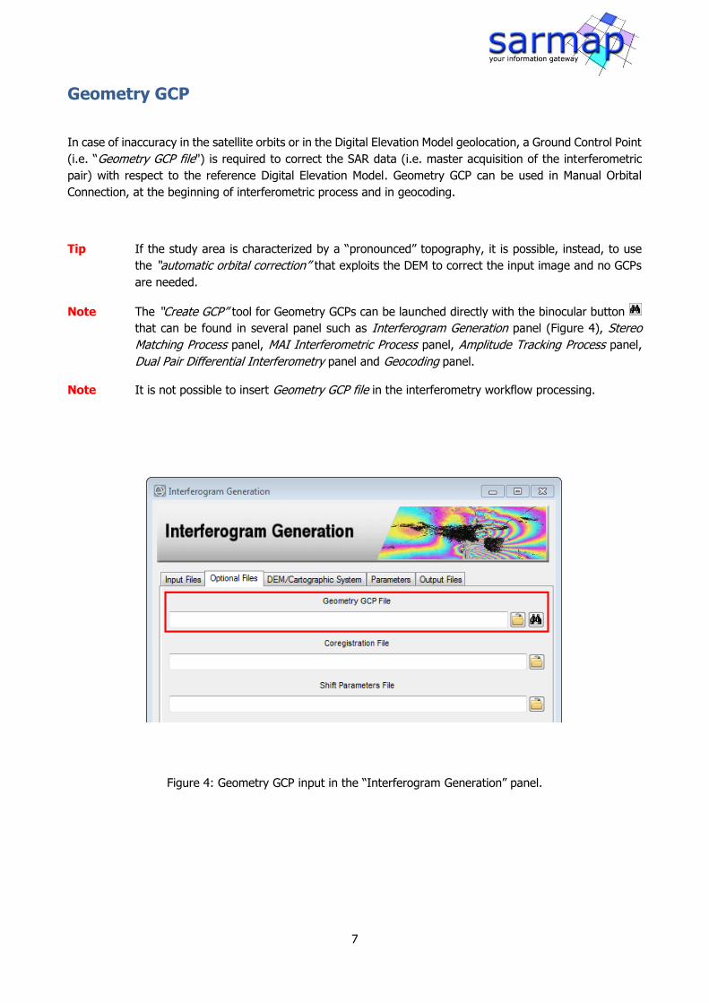
In case of inaccuracy in the satellite orbits or in the Digital Elevation Model geolocation, a Ground Control Point

(i.e. “Geometry GCP file") is required to correct the SAR data (i.e. master acquisition of the interferometric

pair) with respect to the reference Digital Elevation Model. Geometry GCP can be used in Manual Orbital

Connection, at the beginning of interferometric process and in geocoding.

Tip If the study area is characterized by a “pronounced” topography, it is possible, instead, to use

the “automatic orbital correction” that exploits the DEM to correct the input image and no GCPs

are needed.

Note The “Create GCP” tool for Geometry GCPs can be launched directly with the binocular button

that can be found in several panel such as Interferogram Generation panel (Figure 4), Stereo

Matching Process panel, MAI Interferometric Process panel, Amplitude Tracking Process panel,

Dual Pair Differential Interferometry panel and Geocoding panel.

Note It is not possible to insert Geometry GCP file in the interferometry workflow processing.

Figure 4: Geometry GCP input in the “Interferogram Generation” panel.

8

Manual Orbital Correction tool

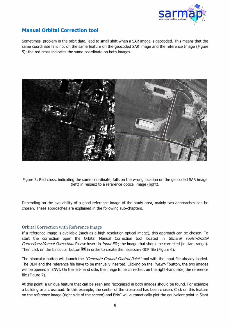
Sometimes, problem in the orbit data, lead to small shift when a SAR image is geocoded. This means that the

same coordinate falls not on the same feature on the geocoded SAR image and the reference Image (Figure

5); the red cross indicates the same coordinate on both images.

Figure 5: Red cross, indicating the same coordinate, falls on the wrong location on the geocoded SAR image

(left) in respect to a reference optical image (right).

Depending on the availability of a good reference image of the study area, mainly two approaches can be

chosen. These approaches are explained in the following sub-chapters.

Orbital Correction with Reference image If a reference image is available (such as a high-resolution optical image), this approach can be chosen. To

start the correction open the Orbital Manual Correction tool located in General Tools>Orbital

Correction>Manual Correction. Please insert in Input File, the image that should be corrected (in slant range).

Then click on the binocular button in order to create the necessary GCP file (Figure 6).

The binocular button will launch the “Generate Ground Control Point” tool with the input file already loaded.

The DEM and the reference file have to be manually inserted. Clicking on the “Next>” button, the two images

will be opened in ENVI. On the left-hand side, the image to be corrected, on the right-hand side, the reference

file (Figure 7).

At this point, a unique feature that can be seen and recognized in both images should be found. For example

a building or a crossroad. In this example, the center of the crossroad has been chosen. Click on this feature

on the reference image (right side of the screen) and ENVI will automatically plot the equivalent point in Slant

9

Range (on the left side of the screen). This point will not be correct projected because of errors in the orbital

information (Figure 8).

At this stage, a GCP will be shown in the GCP list (Figure 9); click on it in order to be able to modify this GCP,

or select the Edit/Modify radio button and then select the GCP on the image. The correct slant range coordinate

can be insert manually or the red “plus” can be moved to the correct location (center of the crossroad) as

shown in Figure 10.

Note Because of the slant range geometry, descending data are flipped west-east and ascending data

are flipped north-south. Therefore, attention should be paid by looking at the same feature in

both images.

Once both crosses are projected on the same feature click “Finish” in the “Create GCPs” panel. This will insert

the created GCP file in the Orbital Correction panel. Click on “Exec” to run it and correct the image. The

corrected slant range image can now be geocoded and there will be no shift (Figure 11).

Figure 6: Manual Orbital Correction Panel (left) and Generate Ground Control Points Panel (right). In the

Generate GCPs panel, the input file is automatically insert. DEM file and reference file have to be manually insert.

10

Input file Reference file

Reference file

Input file

Figure 7: Generate GCP environment with two different geometries on two different views in ENVI. Right: High resolution optical image (reference file), left: slant range image that has to be corrected (input file).

Note: the two separate GCP tree structure in the “Layer Manager”.

Figure 8: Center of the crossroad on the high resolution optical image (green “plus”, right) and its wrong

projection on slant range image (red “plus”, left).

11

Slant range coordinate (automatically insert and displayed on input file on the left, to be corrected)

Geographic coordinate retrived from referencefile

Figure 9: Created GCP in the Generate Ground Control Points panel.

+

Figure 10: Change of position of the red “plus” on the slant range image (left) from the wrong to the correct

position, in order to match the same location of the reference image (green “plus”, right).

12

Figure 11: Red cross, indicating the same coordinate, falls now on the SAR image (left) on the same correct location as on the reference image (optical, right).

Orbital Correction with known coordinates (without Reference Image) Basically, this kind of approach works in the same way as with a reference Image, described in the subchapter

above. In this case only the image to be corrected will be insert in the “Generate Ground Control Points” panel.

A feature with known coordinate should be found and a GCP should be created on it. Then, the correct

coordinate (Latitude, Longitude and Altitude) can be insert (Figure 12). Clicking on “Finish” will then insert the

GCP file in the Orbital Correction Panel. Click “Exec.” To run it and correct the slant range image.

Note If the input file is in slant range, and no “DEM file” is insert, the Cartographic System of the

coordinates insert in the GCP Properties have to be insert in the proper “Cartographic System”

tab. If the DEM has been insert, the coordinates have to be in the same Cartographic System.

13

Insert here latitude, longitude and altitude of the selected knownfeature

Insert here the CartographicSystem of the coordinatesinsert in the GCP propertiesif no «DEM file» has beenselected

Figure 12: GCP created on a known feature. Coordinates and altitude should then be insert in the GCP Properties, its Cartographic System has to be chose in the proper tab if no DEM file has been selected.

14

Refinement GCP

Phase Processing (interferometry)

The refinement GCP file is a mandatory file required for the Refinement step during interferometry process. It

is needed to retrieve phase and unwrapped phase in selected zones.

Ground Control Points for the refinement can be selected either in slant geometry (range and azimuth) or in

geocoded geometry (x, y, h, where the h could be automatically retrieved from the input DEM from the GCP

generation tool), but not in both geometries.

Typically, the GCPs are chosen in slant range. If the GCP are used for more overlapped tracks/frames as

anchor points (Figure 13 shows two examples), they should be taken at their best in geocoded geometry, with

a good coverage of the area where the adjacent tracks overlap. This is important in order to avoid offset

values in phase between different tracks/frames in the same area. The software is hence able to internally

perform a backward geocoding on the slant range geometry used during the refinement.

Figure 13: Examples of overlapping areas.

The most important criteria to select the GCP point’s location on the unwrapped phase files are the following:

There should be no high frequency residual topography fringes

There should be no displacement fringes, hence remain quite far from the displacement area, if known.

The displacement rate of the selected GCPs is considered to be 0, unless a known displacement rate is provided in input, as for example as resulting from external measurements (see proper chapter at

page 25

15

There should be no phase jumps corresponding to unwrapping errors. If a point is located inside an

isolated phase “island”, with poorly unwrapped value, it might be considered as part of a phase ramp

and resulting in an overall wrong correction. If the fint shows systematic acquisition geometry errors (orbit imprecision), the GCPs should then

cover the entire track/frame (always following the criteria listed above) in order to remove this effect.

Once the Generate Control Points tool, found in General Tools, has been launched, the following panel appears

(Figure 14) where _upha, _dem and _fint files have to be insert. Afterwards, click Next > to continue with the

GCP generation.

Note During interferometric workflows (for instance: InSAR DEM Workflow, DInSAR Displacement

Workflow, …), or in general if the GCP is created with the binocular button , the three input

files are automatically chosen if the paths are already insert in the panel.

Figure 14: Generate Ground Control Points, File selection panel.

At this point, the GCP tool will open the _upha and the _fint images in ENVI. It is possible to switch from one

image to the other in the same way as during a normal ENVI session using the checkboxes on the left side of

the file name in the Layer Manager (Figure 15). Figure 16 shows how to change the color scale to the fint

image in order to allow better understanding of the phase data.

16

Figure 15: _upha (on the top) and _fint (on the bottom) images automatically opened by the GCP generation tool (here an example for phase to displacement processing).

Figure 16: Right mouse click > Change Color Table > Rainbow allows to better visualize and interpret the

values of the fint image.

As stated before, a good way to choose the GCPs location is to look for a stable zone far away from movement

fringes (Figure 22), phase jumps corresponding to unwrapping error and residual topography fringes. Well

17

flattened areas (homogeneous color on fint) are good candidate zones for GCPs, in addition several points

distributed on the whole scene are needed for DEM creation and to remove systematic acquisition geometry

errors (orbit imprecision). It is suggested to stay away from steep topography and residual topography fringes

and it is recommended to select GCPs on the valleys bottom (Figure 17, Figure 18 and Figure 21).

Note In case of displacement analysis and with absence of systematic acquisition geometry errors

(orbit imprecision), one GCP is sufficient (Figure 22).

Figure 19 (bottom, right) shows an example of unwrapping error. In fact, if a profile along the phase jump is

drawn Figure 20, it can be noticed how in this case the jump measure exactly a 2 cycle.

If it is planned to process the same study area with different geometries (ascending and descending) or

different sensors, it is suggested to geocode both _fint files and create the GCP using these two files so that

the points are located over zones covered by both geometries (Figure 24). To do this, the _fint file of both

geometries should be geocoded.

Note Attention should be paid in this process. Before starting with the GCPs creation, check that in the

study area no unwrapping errors are present.

Examples in Figure 21 and Figure 23 show the effect of refinement step by mean of refinement GCP on orbital

fringes. It is clearly visible how the pronounced phase ramp present on the left image is removed by the

refinement step. In fact, by default the software handles all the GCPs as stable points and compute a phase

component that has to be removed.

18

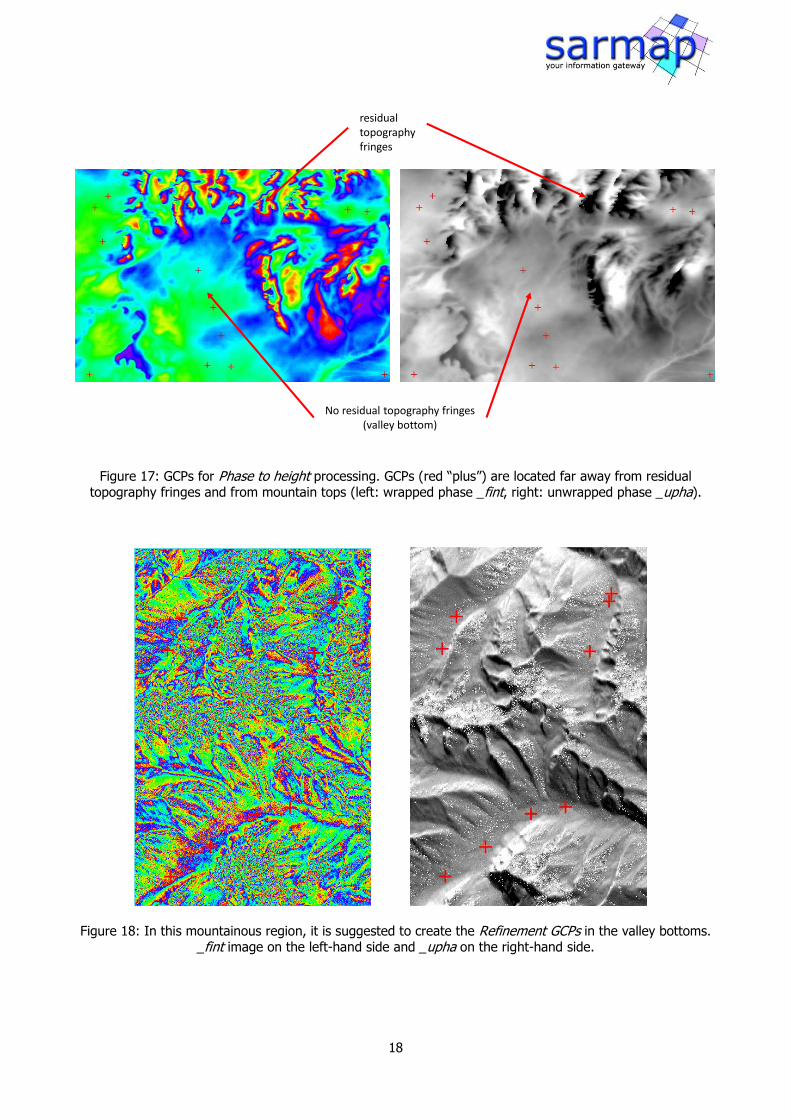
residual topography fringes

No residual topography fringes (valley bottom)

Figure 17: GCPs for Phase to height processing. GCPs (red “plus”) are located far away from residual topography fringes and from mountain tops (left: wrapped phase _fint, right: unwrapped phase _upha).

Figure 18: In this mountainous region, it is suggested to create the Refinement GCPs in the valley bottoms. _fint image on the left-hand side and _upha on the right-hand side.

19

Filtered flattened interferogram

Unwrapped phase showing an “island” where the phase has not been correctly unwrapped

Unwrapped phase showing no errorsPhase Unwrapping

Figure 19: Example of poorly unwrapped data (bottom right), in opposition to good unwrapped data (top right).

Figure 20: Profile crossing an error in the unwrapped phase _upha.

20

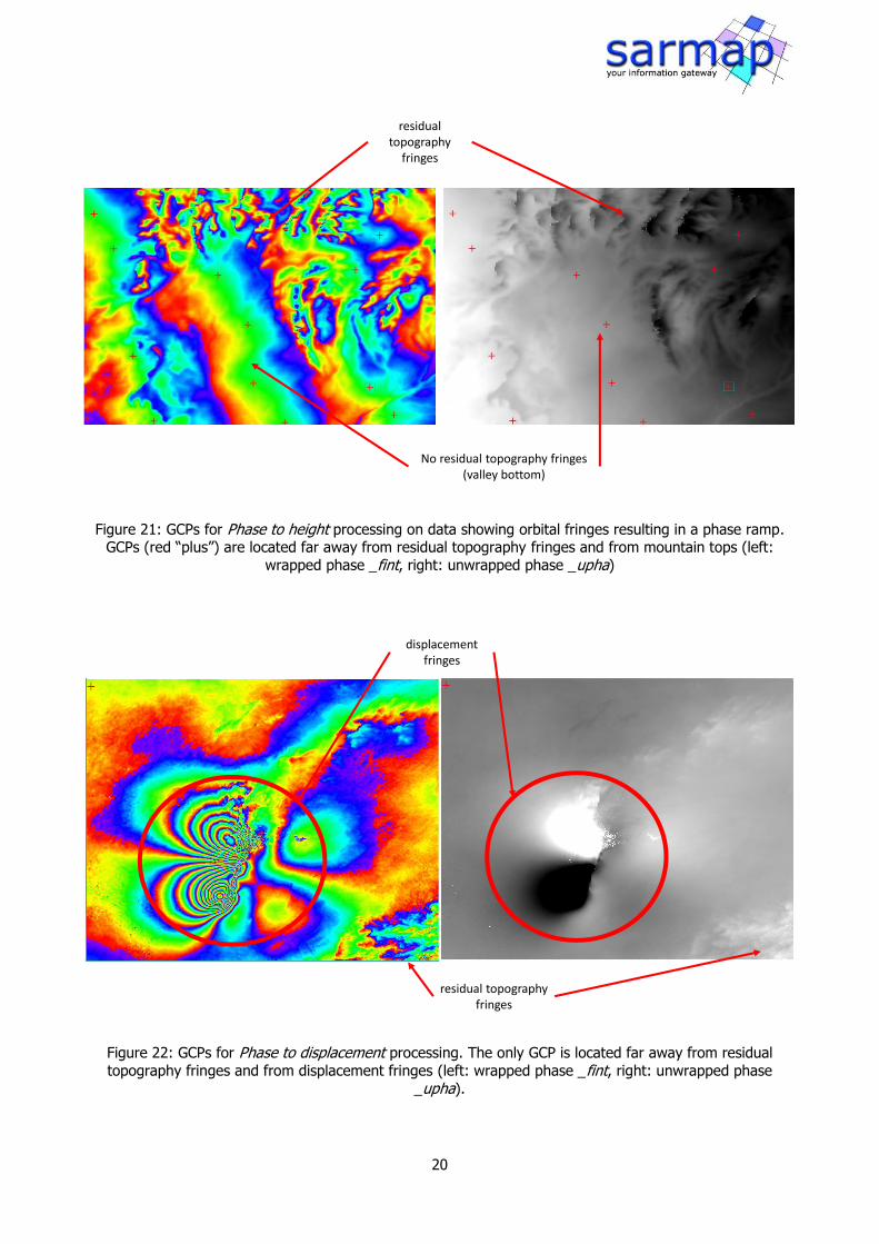
residual topography

fringes

No residual topography fringes (valley bottom)

Figure 21: GCPs for Phase to height processing on data showing orbital fringes resulting in a phase ramp. GCPs (red “plus”) are located far away from residual topography fringes and from mountain tops (left:

wrapped phase _fint, right: unwrapped phase _upha)

residual topography fringes

displacement fringes

Figure 22: GCPs for Phase to displacement processing. The only GCP is located far away from residual

topography fringes and from displacement fringes (left: wrapped phase _fint, right: unwrapped phase

_upha).

21

Ref

inem

ent

by

mea

n o

f R

efin

emen

t G

CP

+++

+

+

+ +

+

+

++

+

+

residual topography fringes

displacement fringes

Figure 23: Example of orbital fringes removing on a flattened interferogram by refinement processing with Refinement GCP (red “plus”). In opposition to Figure 22, more than only 1 point are needed in order to

remove the ramp.

Figure 24: GCPs taken on geocoded _fints from descending (left) and ascending (right) geometries. The

points are located in zones covered by both geometries and not affected by movement and residual

topography fringes.

22

Tip When the Area of Interest is chosen, it is suggested to select a slightly larger area in order to be

sure to have an area outside the displacement area so that it is more likely to select reliable GCPs.

Note For the orbital refinement, at least 7 (valid) GCPs have to be taken. If, instead, a Polynomial

refinement has to be performed, the minimum number of Ground Control Points has to be equal

to the "Residual Phase Poly Degree"; otherwise, the poly degree is automatically decreased

accordingly. For more information, please refer to the Preferences – Flattening and Interferometry

- Phase processing - 4- Refinement and Re-flattening chapter in the SARscape help.

In interferometric stacking

SBAS “refinement and reflattening” step Before starting with the creation of GCPs, a screening of all the fint created by the interferometry step shall

be done in order to identify movement zones in the study area. Then a screening of all the unwrapped phase

shall be done in order to identify errors in the _uphas, these pairs must be removed (please see edit connection

graph in the SBAS tutorial). It is quite difficult to locate GCPs that are all good for all interferograms of the

stack. To start creating the GCPs, open a good _upha showing the movement zones as input file (Figure 25,

left) and an _upha with low surface coverage as reference image (Figure 25, right) in the create GCPs tool

panel and start create the GCPs. The points must be covered by both images and away from movement zones

(Figure 26). Several points shall be insert in order to be sure to have enough valid GCPs because not all _uphas

have the same spatial coverage. Figure 27 shows another example of GCPs selection and the effects on the

reflattened images (Figure 28). The idea is to remove only an average phase or a phase plane where

necessary. For this reason, it is suggested to use always the polynomial refinement method.

Tip A good “rule of thumb” for estimating the amount of GCPs is: the lower the spatial coverage, the

higher the amount of GCPs.

Note It is recommended to not insert points with velocity values in the GCP properties, even if this

velocity is known. Stay rather away from displacement zones and add these points with

displacement data only in the “Inversion second step”.

23

displacement zone

Figure 25: Two _upha of the SBAS interferometric process. On the left: a representative unwrapped phase image showing the displacement zones. On the right: an unwrapped phase image with low surface coverage.

Using these two image as input and reference file in the GCP creation helps in staying away from movement zones and where no data are available.

displacement zone

Figure 26: GCP selection on upha with low spatial coverage. The large amount of points allow to be sure not

having too much points on “Not A Number” zone. Note how there is no GCP on the displacement zone.

24

Figure 27: Flattened filtered interferogram (_fint) on the left and GCPs location over the unwrapped phase on the right. Note how the points are located far away from the displacement zone (in the center) and are

well spread on the whole image in order to remove the phase ramp that is visible in the _fint.

Figure 28: Wrapped (on the left) and unwrapped (on the right) interferogram after the refinement and re-

flattening. The phase ramp has disappeared and the displacement pattern fully remains.

25

SBAS “Inversion second step” and PS “Geocoding” step The Refinement GCPs file in these two steps is used to reflat the results. In case no ramps are left, a single

GCP (one point) can be chosen to remove just a residual phase constant. All the final results will be referred

to these GCPs and they could be called the anchor point(s). For SBAS Inversion second step, the same GCPs

used in the Refinement and Re-Flattening tool might be chosen.

If points with known velocity are available, it is possible to insert this parameter in the GCP properties

(information about the insertion of these data can be found in the proper chapter at page 25).

Note It is suggested to create the Refinement GCPs in geocoded coordinate in order to be able to use

them for both SBAS and PS processing, different geometries (ascending and descending) or

different sensors allowing a direct comparison of the results. This is caused by the use of the

same anchor points in order to avoid offsets between different results.

Known Displacement

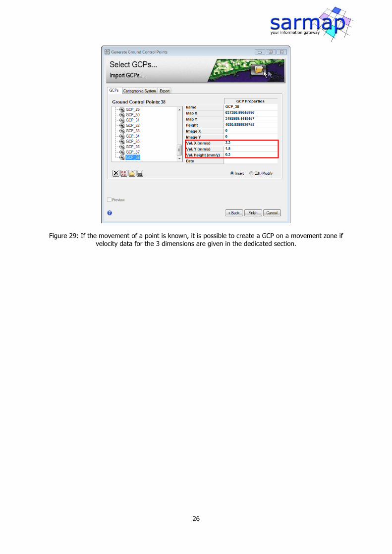
If the displacement rate is known, it is also possible to insert these data directly in the Generate GCPs panel

(Figure 29) in addition to position values. To select a GCP on the image, select firstly the Edit/Modify radio

button.

A positive “Vel. X” value means a movement from west to east

A positive “Vel. Y” value means a movement from south to north

A positive “Vel. Height” value means an uplift

Note The velocity has to be entered for each spatial direction, and it should be given in [mm/y]. If only

the displacement is known, then the velocity has to be calculated taking into account the time

between the two acquisitions. For example a co-seismic displacement of 50 cm for an

interferometric pair acquired at 35 days distance will correspond to a velocity of around 5214

mm/year (500÷35*365). This should then be projected in the tree spatial dimension.

Note It is possible to use data coming from GPS stations. SINEX and GSI format can be imported by

the Import GPS tool (see proper chapter in SARscape help).

26

Figure 29: If the movement of a point is known, it is possible to create a GCP on a movement zone if velocity data for the 3 dimensions are given in the dedicated section.

27

Overview table

Geometry GCP Use Map X and Y Height [m] Image X and Y Velocity X, Y,

Z [mm/y]

Date

Manual Orbital

Correction with

Reference Image

Selected with

Generate GCP

tool

Retrieved from

DEM file

Selected with

Generate GCP

tool

Not used Not used

Manual Orbital

correction with

Known Coordinates

Entered

manually

Entered

manually

Selected with

Generate GCP

tool

Not used Not used

Refinement GCP Use Map X and Y Height [m] Image X and Y Velocity X, Y,

Z [mm/y]

Date

Orbital Refinement

using geographic

Input file

Selected with

Generate GCP

tool or Entered

manually

Retrieved from

DEM file or will

be read in

Refinement and

Reflattening step

or Entered

manually

Will be

calculated from

the software in

Refinement and

Reflattening step

Not used Not used

Orbital Refinement

using Input file in sar

geometry

Not used Not used Selected with

Generate GCP

tool

Not used Not used

Orbital Refinement

combined with

known velocity

Selected with

Generate GCP

tool or Entered

manually

Retrieved from

DEM file or will

be read in

Refinement and

Reflattening step

or Entered

manually

Will be

calculated from

the software in

Refinement and

Reflattening step

Entered

manually

Entered

manually

Orbital Refinement

combined with

known velocity

coming from GPS

stations (SINEX and

GSI)

Note: This file will be

created with the

Import GPS tool

instead of the Create

GCP tool

Entered by the

Import GPS tool

Entered by the

Import GPS tool

Entered by the

Import GPS tool

Entered by the

Import GPS

tool

Entered by

the Import

GPS tool