Embed Size (px)
Citation preview
GAZETA MATEMATICA
SERIA A
ANUL XXXIV (CXIII) Nr. 1 – 2/ 2016
ARTICOLE
On a two parameter class of quadratic Diophantine equations
Arpad Benyi1), 2), Ioan Casu3)
Abstract. We characterize the solution set of a two parameter class ofquadratic Diophantine equations. Our proof relies on the solvability of thepositive Pell equation.
Keywords: Diophantine equation, quadratic equation, Pell equation
MSC: Primary 11D09; Secondary 40-01.
In this note we will be interested in exploring the solutions of quadraticDiophantine equations of the form
ax2 + by2 + cx+ dy + f = 0,
where a, b, c, d, f ∈ Z. Naturally, there is no hope in solving such a problemfor arbitrary coefficients, and simple examples show that there are such equa-tions which have zero, finitely many or infinitely many solutions (x, y) ∈ Z×Z.Equivalently, we can see this to be the case by inspecting the lattice pointssitting on the algebraic curve defined by the quadratic equation above, butthis geometric intuition is not the one we will be using here. Our motiva-tion for this note stems from the following two problems proposed at the 7–8grade level:
[3]. Let a, b ∈ N be such that 4a2 + 9a + 1 = 3b2 + 7b. Show that3a+ 3b+ 7 and 4a+ 4b+ 9 are perfect squares.
[4]. Let x, y ∈ N such that x > y and x + 4x2 = y + 5y2. Show thatx− y is a perfect square.
1)Department of Mathematics, WesternWashington University, 516 High Street, Belling-ham, Washington 98225, USA, [email protected]
2)This work is partially supported by a grant from the Simons Foundation (No. 246024
to Arpad Benyi)3)Department of Mathematics, West University of Timisoara, Romania,
2 Articole
We wish to show that the intuition behind these problems lends itselfnicely to completely solving a two parameter class of quadratic Diophantineequations. Specifically, let α, β ∈ N∪0 and consider the following equationin variables (x, y) ∈ Z× Z:
αx2 − (α+ 1)y2 + (2αβ + 1)x− (2αβ + 2β + 1)y − β2 = 0. (1)
Clearly, for α = 3 and β = 1 we obtain the equation in [3], while for α = 4,β = 0 we get the equation in [4].
Let us remark right away that when α = 0, the equation (1) reducesto x = y2 + (2β + 1)y + β2, which already produces the parametrizationfor all the infinitely many integer solutions of the equation. In fact, slightlyre-writing, we have in this case x = (y + β)2 + y, y ∈ Z, which suggeststhat understanding the solutions of the two parameter Diophantine equation(1) could potentially be reduced to the solutions of just a one parameterDiophantine equation by appropriately substituting for x and y. We showfirst that this is indeed the case.
Reduction to a one parameter Diophantine equation. Let us makethe change of variables
X = x+ β and Y = y + β.
Thus, replacing x = X − β and y = Y − β in (1) we obtain
α(X−β)2−(α+1)(Y −β)2+(2αβ+1)(X−β)−(2αβ+2β+1)(Y −β) = β2,
which after some straightforward algebra simplifies to
αX2 − (α+ 1)Y 2 +X − Y = 0.
This simply means that in the two parameter Diophantine equation (1) wecan assume without loss of generality β = 0. Moreover, if a solution of (1)exists for β = 0, the general solution for β 6= 0 is obtained from that one bytranslating by −β in both unknowns.
Note also that if we let α = 0 and β = 0 in (1), we already have theparametrization of all the integer solutions: x = y2 − y, with y ∈ Z. Withthese considerations, we will assume in the remainder of this note that α ∈ Nand β = 0 in (1), that is we will investigate the integer solutions of
αx2 − (α+ 1)y2 + x− y = 0. (2)
Our main result is the following.
Theorem 1. Let α ∈ N. The non-trivial solutions (xn, yn)n≥1 of the qua-dratic Diophantine equation (2) are given by
xn = (α+ 1)v2n ± unvn, yn = αv2n ± unvn,
where
un =(√α+ 1 +
√α)2n + (
√α+ 1−√
α)2n
2,
A. Benyi, I. Casu, Quadratic Diophantine equations 3
vn =(√α+ 1 +
√α)2n − (
√α+ 1−√
α)2n
2√
α(α+ 1).
Moreover, the solution set of (1) is given by(xn − β, yn − β) : n ∈ N ∪ (−β,−β),
with xn, yn as above.
The word “trivial” above refers to the pair (0, 0) which obviously satis-fies the given equation. We point out also that the ± signs in the expressionsof xn and yn, respectively, coincide. We have the following immediate conse-quence of our main result.
Corollary 2. Let (x, y) ∈ Z be a solution of (2). Then x − y is a perfectsquare and the values of x− y belong precisely to the set
0 ∪ v2n : n ∈ N,with vn defined in Theorem 1.
Note that, in particular, we recover the statement in [4]. In fact, the ideaof proving Theorem 1 is guided by the intuition contained in the elementaryproblems [3] and [4], combined with the well-understood theory of positivePell equations. As we shall see, the statement in [3] is also a by-product ofour arguments showing the main result. Before proceeding with the proof ofTheorem 1, we take a brief excursion into the theory of Pell equations.
The general positive Pell equation. Let D be a positive integer that isnot a perfect square. It is a known fact that the positive Pell equation
u2 −Dv2 = 1 (3)
has infinitely many solutions in Z×Z. Clearly, if (u, v) ∈ N×N is a solutionto the Pell equation, then (u,−v), (−u, v) and (−u,−v) are also solutions.Thus, without loss of generality, it suffices to consider only its solutions in thenatural lattice. Any equation of the form (3) has the trivial solution (1, 0).Besides the trivial solution, the other solutions in the natural lattice can beobtained from the fundamental solution (u0, v0), which is the least positiveinteger solution to (3) different from (1, 0) — the so-called fundamental so-
lution of (3) for which the expression u+ v√D is minimal, via the following
formulas:
un =(u0 + v0
√D)n + (u0 − v0
√D)n
2
vn =(u0 + v0
√D)n − (u0 − v0
√D)n
2√D
,n ∈ N.
For a brief introduction to Pell equations, the interested reader can consult,for example, [1] and the references therein.
With these prerequisites we are ready to proceed with the proof of ourmain result.
4 Articole
Proof of Theorem 1. In what follow, we assume that both unknowns, xand y, are non-zero. In particular, this means that x 6= y.
Our first claim, following the statement in [4], is that if x, y satisfy (2),then x− y must be a perfect square. Let us start by re-writing the equation(2) in two ways:
(x− y)[1 + α(x+ y)] = y2,
(x− y)[1 + (α+ 1)(x+ y) = x2.
Denoting A = 1+α(x+ y) and B = 1+(α+1)(x+ y) and multiplying thesetwo equations we obtain (x − y)2AB = (xy)2, thus showing that AB mustbe a perfect square. In particular, we find that A and B must be either bothpositive or both negative.
Let us assume for the moment that both A and B are positive. Notenow that (α+1)A−αB = 1. Therefore, A and B are relatively prime naturalnumbers. Combining this with the fact that AB is a perfect square showsthat A and B have to be perfect squares as well; this is a simple consequenceof the Fundamental Theorem of Arithmetic. Incidentally, the statement thatA and B must be perfect squares is precisely the content of the problem [3]if we take into account also the natural change of variables reducing (1) to(2). Now, since A is a perfect square and (x − y)A is a perfect square, weconclude that x− y > 0 must also be a perfect square. This proves our firstclaim.
With this information in hand, let us write then x − y = v2 for somev ∈ N. Our next claim is that v must be of the form vn, n ≥ 1, with vn as inthe statement of our Theorem 1. Substituting x = y+ v2 in (2) we find that
α(y + v2)2 − (α+ 1)y2 + v2 = 0 ⇔ y2 − 2αv2y − (αv4 + v2) = 0.
We are interested in the integer solutions of the quadratic equation in y,which are given by
y = αv2 ± v√
α(α+ 1)v2 + 1. (4)
Clearly, for y to be an integer, we need now
α(α+ 1)v2 + 1 = u2 ⇔ u2 − α(α+ 1)v2 = 1, (5)
for some u ∈ Z. But this is exactly a positive Pell equation of the form (3),with D = α(α + 1) obviously not being a perfect square. It is equally easyto see that the fundamental solution of (5) is given by
u0 = 2α+ 1, v0 = 2.
Thus, the general solution of (5) in N× N can be expressed as
un =(2α+ 1 + 2
√α(α+ 1))n + (2α+ 1− 2
√α(α+ 1))n
2,
A. Benyi, I. Casu, Quadratic Diophantine equations 5
vn =(2α+ 1 + 2
√α(α+ 1))n − (2α+ 1− 2
√α(α+ 1))n
2√
α(α+ 1).
It is straightforward to see that these expressions are precisely the ones statedin Theorem 1, since
2α+ 1± 2√α(α+ 1) = (
√α+ 1±√
α)2.
Returning now to the formula (4), we thus find that the integer solutions areprecisely those of the form yn = αv2n ± vnun, and consequently
xn = y2n + v2n = (α+ 1)v2n ± vnun.
In the argument above, we assumed that both A and B are strictlypositive. The remainder of our proof will show that the scenario in which A
and B are both negative cannot happen. Note that if A,B would be negative,then −A and −B would be positive and since A and B are relatively prime,so are −A and −B, thus implying that −A and −B are perfect squares.Hence, since (y − x)(−A) = y2, we conclude now that y − x > 0 must be aperfect square.
It is worth noting that if y > x and x > 0, the Diophantine equation(2) has no solutions. Indeed, in this case
αx2 − (α+ 1)y2 + x− y < αy2 − (α+ 1)y2 = −y2 < 0.
Thus, the only possible solutions would have to have x < 0. Substitutingy = x+ w2 in (2) we arrive to
αx2 − (α+ 1)(x+ w2)2 − w2 = 0.
This is now equivalent to
x2 + 2(α+ 1)xw2 + (α+ 1)w4 + w2 = 0,
and solving for x gives
x = −(α+ 1)w2 ±√
(α+ 1)2w4 − (α+ 1)w4 − w2 =
= −(α+ 1)w2 ± w√α(α+ 1)w2 − 1.
Therefore, clearly, if x ∈ Z, it must be negative. We stumble here across asimilar issue as in the first part of our argument, except that now me mustrequire
α(α+ 1)w2 − 1 = z2 ⇔ z2 − α(α+ 1)w2 = −1
for some z ∈ Z. This is an example of a negative Pell equation
z2 −Dw2 = −1, (6)
with D = α(α+ 1) not a perfect square. Now, it is well known [2, Theorem3.3.4] that the negative Pell equation (6) is solvable if and only if the period
of the continued fraction expansion of√D is odd. For the fact that, for D
6 Articole
not a perfect square, the continued fraction expansion of√D is periodic, see
[2, Theorem 2.1.21]. Notice next that we have the following identity√α(α+ 1)− α =
α
α+√α(α+ 1)
.
Equivalently, the continued fraction expansion of√α(α+ 1) is given by
√α(α+ 1) = α+
α
2α+ α2α+ α
...
= [α;α, 2α].
We have thus obtained that the period of the continued fraction expansion of√D =
√α(α+ 1) is even, effectively showing that (6) above has no integer
solutions. We conclude that we cannot have solutions (x, y) of (2) with x < y,thus finishing the proof of our main theorem.
Acknowledgment. The authors would like to thank the anonymous refereefor pointing out an error in the manuscript and very useful comments whichsignificantly improved the presentation.
References
[1] T. Andreescu, D. Andrica, I. Cucurezeanu, An Introduction to Diophantine Equations,Springer Verlag, 2010.
[2] T. Andreescu, D. Andrica, Quadratic Diophantine Equations, Springer, 2015.[3] M. Chirita, Problema E:14405, Gazeta Matematica (Seria B) 117 (2012), nr. 1.[4] N. Stanciu, I. Trasca, Problema E:14871, Gazeta Matematica (Seria B) 120 (2015), nr.
6-7-8.
Limits of integrals of functions over various domains
Dumitru Popa1)
Abstract. We prove that, under natural hypotheses, the following equalityholds
limn→∞
nk
∫ 1
0
vn (x)ϕ (x)k∏
i=1
(
n
√
fi (x)− 1)
dx
= limn→∞
∫ 1
0
vn (x)ϕ (x)
k∏
i=1
ln fi (x) dx.
We also show that the main ideas of the proof of this result can be adaptedto obtain a similar result on the unit square. Various applications aregiven.
Keywords: Riemann integral, multiple Riemann integral, the limit ofsequences of multiple integrals
MSC: Primary 26B15; Secondary 28A35.
1)Department of Mathematics, Ovidius University of Constanta, Bd. Mamaia 124,900527 Constanta, Romania, [email protected]
D. Popa, Limits of integrals of functions over various domains 7
1. Introduction and a preliminary result
The starting point for this paper was the following question: how canwe obtain some analogous results to the following limit
limn→∞
n2
∫ 1
0
(n√1 + xn − 1
)dx =
π2
12(1)
given at Vojtech Jarnık International Mathematical Competition 2002, andproposed by Sofia University St. Kliment Ohridski; see [4]. The result ofthis investigation is the present paper. Let us mention that the notation andconcepts used and not defined are standard, see [1]. We need the followingwell-known result whose proof is left to the reader.
Proposition 1. If M > 0, then
0 ≤ ea − 1 ≤ eM − 1
M· a, ∀ 0 ≤ a ≤ M ;
0 ≤ ea − 1− a ≤ eM − 1−M
M2· a2, ∀ 0 ≤ a ≤ M.
2. An illustrative particular case
We begin by proving the first result which the author has obtainedmotivated by the limit (1). Since, shortly after proving this particular resultwe have observed that this can be extended to very general situations wethink that it is instructive for the readers to present first this particular case.
Proposition 2. The following equality holds
limn→∞
n2
∫ 1
0xn(
n√1 + x− 1
)dx = ln 2.
Proof. The idea is to observe that n√1 + x = e
1nln(1+x) and to use Proposition
1, which was expanded to the following reasoning. Let n ∈ N and x ∈ [0, 1].Then 0 ≤ a = 1
n ln (1 + x) ≤ 1n ln 2 ≤ 1
n ≤ 1 and by Proposition 1 we deduce
0 ≤ n√1 + x− 1− 1
nln (1 + x) = e
1nln(1+x) − 1− 1
nln (1 + x)
≤ e− 2
n2ln2 (1 + x) ≤ (e− 2) ln2 2
n2.
By multiplication with n2xn we obtain
0 ≤ n2xn(
n√1 + x− 1− 1
nln (1 + x)
)≤ (e− 2)xn ln2 2
and
0 ≤ n2
∫ 1
0xn(
n√1 + x− 1− 1
nln (1 + x)
)dx ≤ (e− 2) ln2 2
∫ 1
0xndx → 0.
8 Articole
From the equality
n2xn(
n√1 + x− 1
)= n2xn
(n√1 + x− 1− 1
nln (1 + x)
)+ nxn ln (1 + x)
we deduce
n2
∫ 1
0xn(
n√1 + x− 1
)dx
= n2
∫ 1
0xn(
n√1 + x− 1− 1
nln (1 + x)
)dx+ n
∫ 1
0xn ln (1 + x) dx.
Since, as it is well known, n∫ 10 xn ln (1 + x) dx → ln 2, the proof is finished.
Second proof. The following proof has been shown to us by the reviewer.Integrating by parts we have∫ 1
0xn(
n√1 + x− 1
)dx =
xn+1(
n√1 + x− 1
)
n+ 1|10 −
− 1
n (n+ 1)
∫ 1
0(1 + x)
1n−1 xn+1dx
=n√2− 1
n+ 1− 1
n (n+ 1)
∫ 1
0(1 + x)
1n−1 xn+1dx.
It follows that
n2
∫ 1
0xn(
n√1 + x− 1
)dx =
n2(
n√2− 1
)
n+ 1− n
n+ 1
∫ 1
0(1 + x)
1n−1 xn+1dx.
The limit follows since n(
n√2− 1
)→ ln 2 and
0 <
∫ 1
0(1 + x)
1n−1 xn+1dx ≤
n√2
n+ 2.
2
3. The case of Riemann integrable functions on the unitinterval: the first step
The main feature of the proof of Proposition 2 is that it can be extendedto more general context.
Theorem 3. Let vn : [0, 1] → R be a sequence of Riemann integrable func-
tions such that the sequence(∫ 1
0 |vn (x)| dx)n∈N
is bounded. Then for each
Riemann integrable function ϕ : [0, 1] → R and each continuous functionf : [0, 1] → [1,∞) the following equality holds
limn→∞
[n
∫ 1
0vn (x)
(n√f (x)− 1
)ϕ (x) dx−
∫ 1
0vn (x)ϕ (x) ln f (x) dx
]= 0.
In particular, if limn→∞
∫ 10 vn (x)ϕ (x) ln f (x) dx ∈ R, then
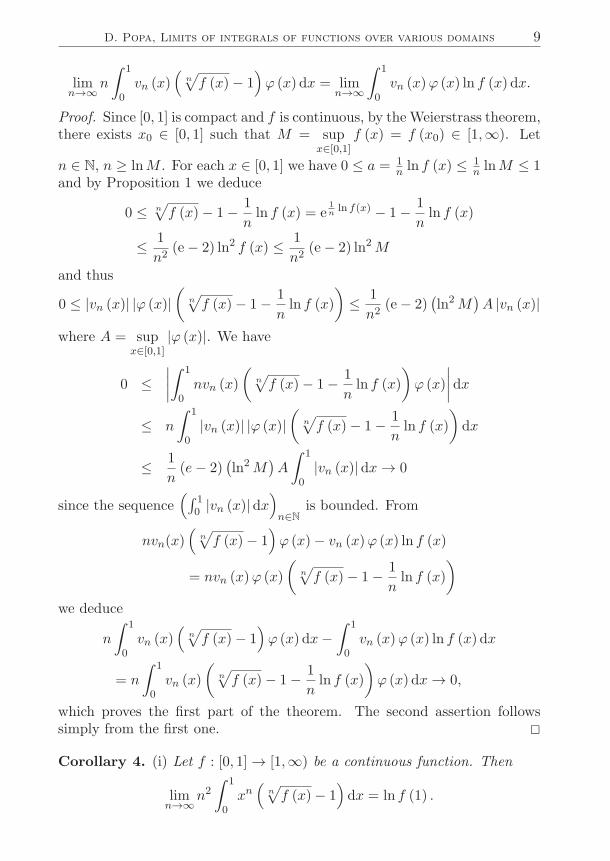
D. Popa, Limits of integrals of functions over various domains 9
limn→∞
n
∫ 1
0vn (x)
(n√
f (x)− 1)ϕ (x) dx = lim
n→∞
∫ 1
0vn (x)ϕ (x) ln f (x) dx.
Proof. Since [0, 1] is compact and f is continuous, by theWeierstrass theorem,there exists x0 ∈ [0, 1] such that M = sup
x∈[0,1]f (x) = f (x0) ∈ [1,∞). Let
n ∈ N, n ≥ lnM . For each x ∈ [0, 1] we have 0 ≤ a = 1n ln f (x) ≤ 1
n lnM ≤ 1and by Proposition 1 we deduce
0 ≤ n√f (x)− 1− 1
nln f (x) = e
1nln f(x) − 1− 1
nln f (x)
≤ 1
n2(e− 2) ln2 f (x) ≤ 1
n2(e− 2) ln2M
and thus
0 ≤ |vn (x)| |ϕ (x)|(
n√f (x)− 1− 1
nln f (x)
)≤ 1
n2(e− 2)
(ln2M
)A |vn (x)|
where A = supx∈[0,1]
|ϕ (x)|. We have
0 ≤∣∣∣∣∫ 1
0nvn (x)
(n√f (x)− 1− 1
nln f (x)
)ϕ (x)
∣∣∣∣ dx
≤ n
∫ 1
0|vn (x)| |ϕ (x)|
(n√f (x)− 1− 1
nln f (x)
)dx
≤ 1
n(e− 2)
(ln2M
)A
∫ 1
0|vn (x)| dx → 0
since the sequence(∫ 1
0 |vn (x)| dx)n∈N
is bounded. From
nvn(x)(
n√f (x)− 1
)ϕ (x)− vn (x)ϕ (x) ln f (x)
= nvn (x)ϕ (x)
(n√f (x)− 1− 1
nln f (x)
)
we deduce
n
∫ 1
0vn (x)
(n√f (x)− 1
)ϕ (x) dx−
∫ 1
0vn (x)ϕ (x) ln f (x) dx
= n
∫ 1
0vn (x)
(n√f (x)− 1− 1
nln f (x)
)ϕ (x) dx → 0,
which proves the first part of the theorem. The second assertion followssimply from the first one. 2
Corollary 4. (i) Let f : [0, 1] → [1,∞) be a continuous function. Then
limn→∞
n2
∫ 1
0xn(
n√f (x)− 1
)dx = ln f (1) .
10 Articole
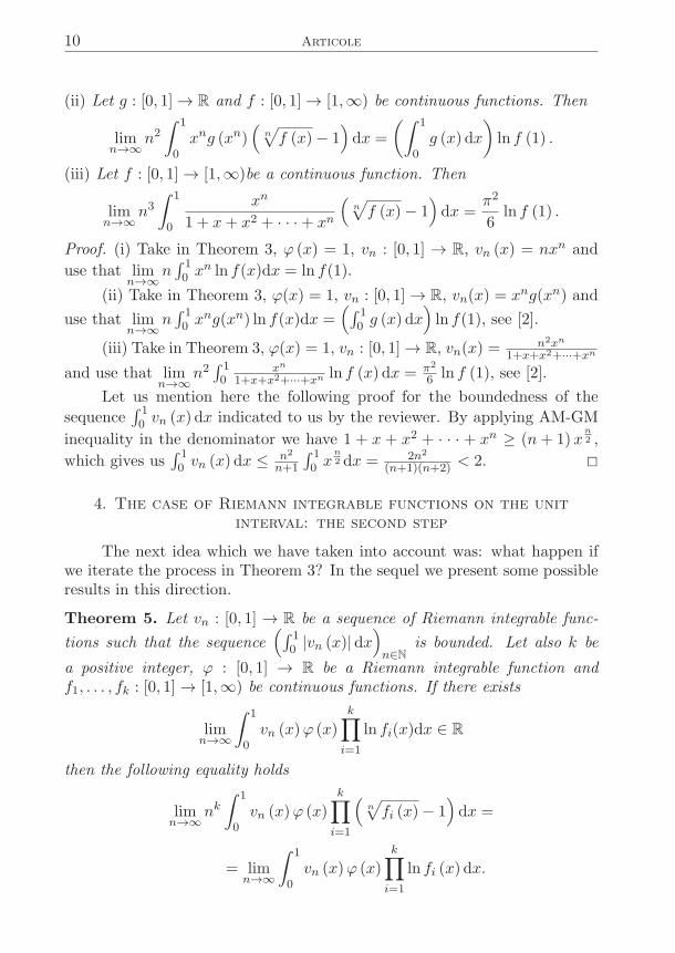
(ii) Let g : [0, 1] → R and f : [0, 1] → [1,∞) be continuous functions. Then
limn→∞
n2
∫ 1
0xng (xn)
(n√f (x)− 1
)dx =
(∫ 1
0g (x) dx
)ln f (1) .
(iii) Let f : [0, 1] → [1,∞)be a continuous function. Then
limn→∞
n3
∫ 1
0
xn
1 + x+ x2 + · · ·+ xn
(n√f (x)− 1
)dx =
π2
6ln f (1) .
Proof. (i) Take in Theorem 3, ϕ (x) = 1, vn : [0, 1] → R, vn (x) = nxn and
use that limn→∞
n∫ 10 xn ln f(x)dx = ln f(1).
(ii) Take in Theorem 3, ϕ(x) = 1, vn : [0, 1] → R, vn(x) = xng(xn) and
use that limn→∞
n∫ 10 xng(xn) ln f(x)dx =
(∫ 10 g (x) dx
)ln f(1), see [2].
(iii) Take in Theorem 3, ϕ(x) = 1, vn : [0, 1] → R, vn(x) = n2xn
1+x+x2+···+xn
and use that limn→∞
n2∫ 10
xn
1+x+x2+···+xn ln f (x) dx = π2
6 ln f (1), see [2].
Let us mention here the following proof for the boundedness of the
sequence∫ 10 vn (x) dx indicated to us by the reviewer. By applying AM-GM
inequality in the denominator we have 1 + x + x2 + · · · + xn ≥ (n+ 1)xn
2 ,
which gives us∫ 10 vn (x) dx ≤ n2
n+1
∫ 10 x
n
2 dx = 2n2
(n+1)(n+2) < 2. 2
4. The case of Riemann integrable functions on the unitinterval: the second step
The next idea which we have taken into account was: what happen ifwe iterate the process in Theorem 3? In the sequel we present some possibleresults in this direction.
Theorem 5. Let vn : [0, 1] → R be a sequence of Riemann integrable func-
tions such that the sequence(∫ 1
0 |vn (x)| dx)n∈N
is bounded. Let also k be
a positive integer, ϕ : [0, 1] → R be a Riemann integrable function andf1, . . . , fk : [0, 1] → [1,∞) be continuous functions. If there exists
limn→∞
∫ 1
0vn (x)ϕ (x)
k∏
i=1
ln fi(x)dx ∈ R
then the following equality holds
limn→∞
nk
∫ 1
0vn (x)ϕ (x)
k∏
i=1
(n√fi (x)− 1
)dx =
= limn→∞
∫ 1
0vn (x)ϕ (x)
k∏
i=1
ln fi (x) dx.
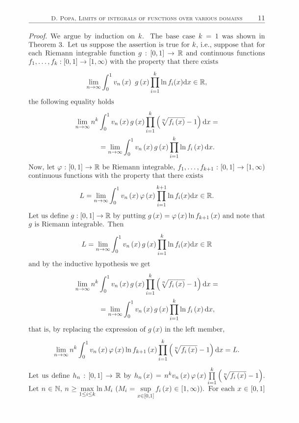
D. Popa, Limits of integrals of functions over various domains 11
Proof. We argue by induction on k. The base case k = 1 was shown inTheorem 3. Let us suppose the assertion is true for k, i.e., suppose that foreach Riemann integrable function g : [0, 1] → R and continuous functionsf1, . . . , fk : [0, 1] → [1,∞) with the property that there exists
limn→∞
∫ 1
0vn (x) g (x)
k∏
i=1
ln fi(x)dx ∈ R,
the following equality holds
limn→∞
nk
∫ 1
0vn (x) g (x)
k∏
i=1
(n√
fi (x)− 1)dx =
= limn→∞
∫ 1
0vn (x) g (x)
k∏
i=1
ln fi (x) dx.
Now, let ϕ : [0, 1] → R be Riemann integrable, f1, . . . , fk+1 : [0, 1] → [1,∞)continuous functions with the property that there exists
L = limn→∞
∫ 1
0vn (x)ϕ (x)
k+1∏
i=1
ln fi(x)dx ∈ R.
Let us define g : [0, 1] → R by putting g (x) = ϕ (x) ln fk+1 (x) and note thatg is Riemann integrable. Then
L = limn→∞
∫ 1
0vn (x) g (x)
k∏
i=1
ln fi(x)dx ∈ R
and by the inductive hypothesis we get
limn→∞
nk
∫ 1
0vn (x) g (x)
k∏
i=1
(n√
fi (x)− 1)dx =
= limn→∞
∫ 1
0vn (x) g (x)
k∏
i=1
ln fi (x) dx,
that is, by replacing the expression of g (x) in the left member,
limn→∞
nk
∫ 1
0vn (x)ϕ (x) ln fk+1 (x)
k∏
i=1
(n√fi (x)− 1
)dx = L.
Let us define hn : [0, 1] → R by hn (x) = nkvn (x)ϕ (x)k∏
i=1
(n√
fi (x)− 1).
Let n ∈ N, n ≥ max1≤i≤k
lnMi (Mi = supx∈[0,1]
fi (x) ∈ [1,∞)). For each x ∈ [0, 1]
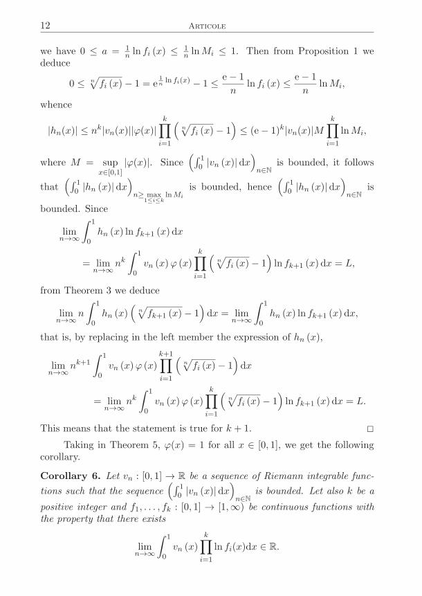
12 Articole
we have 0 ≤ a = 1n ln fi (x) ≤ 1
n lnMi ≤ 1. Then from Proposition 1 wededuce
0 ≤ n√fi (x)− 1 = e
1nln fi(x) − 1 ≤ e− 1
nln fi (x) ≤
e− 1
nlnMi,
whence
|hn(x)| ≤ nk|vn(x)||ϕ(x)|k∏
i=1
(n√fi (x)− 1
)≤ (e− 1)k|vn(x)|M
k∏
i=1
lnMi,
where M = supx∈[0,1]
|ϕ(x)|. Since(∫ 1
0 |vn (x)| dx)n∈N
is bounded, it follows
that(∫ 1
0 |hn (x)| dx)n≥ max
1≤i≤k
lnMi
is bounded, hence(∫ 1
0 |hn (x)| dx)n∈N
is
bounded. Since
limn→∞
∫ 1
0hn (x) ln fk+1 (x) dx
= limn→∞
nk
∫ 1
0vn (x)ϕ (x)
k∏
i=1
(n√fi (x)− 1
)ln fk+1 (x) dx = L,
from Theorem 3 we deduce
limn→∞
n
∫ 1
0hn (x)
(n√fk+1 (x)− 1
)dx = lim
n→∞
∫ 1
0hn (x) ln fk+1 (x) dx,
that is, by replacing in the left member the expression of hn (x),
limn→∞
nk+1
∫ 1
0vn (x)ϕ (x)
k+1∏
i=1
(n√fi (x)− 1
)dx
= limn→∞
nk
∫ 1
0vn (x)ϕ (x)
k∏
i=1
(n√fi (x)− 1
)ln fk+1 (x) dx = L.
This means that the statement is true for k + 1. 2
Taking in Theorem 5, ϕ(x) = 1 for all x ∈ [0, 1], we get the followingcorollary.
Corollary 6. Let vn : [0, 1] → R be a sequence of Riemann integrable func-
tions such that the sequence(∫ 1
0 |vn (x)| dx)n∈N
is bounded. Let also k be a
positive integer and f1, . . . , fk : [0, 1] → [1,∞) be continuous functions withthe property that there exists
limn→∞
∫ 1
0vn (x)
k∏
i=1
ln fi(x)dx ∈ R.
D. Popa, Limits of integrals of functions over various domains 13
Then the following equality holds
limn→∞
nk
∫ 1
0vn (x)
k∏
i=1
(n√fi (x)− 1
)dx = lim
n→∞
∫ 1
0vn (x)
k∏
i=1
ln fi(x)dx.
We recall a well known result, see [2, Ex. 3.13, pag. 53–54].
Lemma 7. Let vn : [0, 1] → R be a sequence of Riemann integrable functions
such that the sequence(∫ 1
0 |vn (x)| dx)n∈N
is bounded, an for all 0 < u < 1
we have limn→∞
∫ u0 |vn (x)| dx = 0 and lim
n→∞
∫ 10 vn (x) dx ∈ R. Then for each
continuous function f : [0, 1] → R the following equality holds
limn→∞
∫ 1
0vn (x) f (x) dx = f (1) lim
n→∞
∫ 1
0vn (x) dx.
From Corollary 6 and Lemma 7 we get the following result which is anextension of Proposition 2 and Corollary 4.
Corollary 8. Let vn : [0, 1] → R be a sequence of Riemann integrable
functions such that the sequence(∫ 1
0 |vn (x)| dx)n∈N
is bounded, and for all
0 < u < 1 we have limn→∞
∫ u0 |vn (x)| dx = 0 and lim
n→∞
∫ 10 vn (x) dx ∈ R. Let
also k be a positive integer and f1, . . . , fk : [0, 1] → [1,∞) be continuousfunctions. Then the following equality holds
limn→∞
nk
∫ 1
0vn (x)
k∏
i=1
(n√
fi (x)− 1)dx =
[k∏
i=1
ln fi (1)
]limn→∞
∫ 1
0vn (x) dx.
Taking in Theorem 5, vn (x) = 1 for all x ∈ [0, 1] and n ∈ N, we get thefollowing corollary.
Corollary 9. Let k be a positive integer, ϕ : [0, 1] → R a Riemann integrablefunction and f1, . . . , fk : [0, 1] → [1,∞) continuous functions. Then thefollowing equality holds
limn→∞
nk
∫ 1
0ϕ (x)
k∏
i=1
(n√fi (x)− 1
)dx =
∫ 1
0ϕ (x)
k∏
i=1
ln fi (x) dx.
Corollary 10. For each positive integer k the following equality holds
limn→∞
nk
∫ 1
0
(n√1 + x− 1
)kdx = Ik,
where I1 = 2 ln 2− 1, Ik = 2 lnk 2− kIk−1, for k ≥ 2, and Ik are as above.
Proof. From Corollary 9 we have
limn→∞
nk
∫ 1
0
(n√1 + x− 1
)kdx =
∫ 1
0[ln (1 + x)]k dx = Ik.
It is a standard exercise to prove that Ik has the stated properties. 2
14 Articole
5. The case of Riemann integrable functions on the unit square
In the sequel we show that, following similar ideas, we can prove thatTheorems 3 and 5 can be extended to Riemann integrable functions on theunit square.
Theorem 11. Let hn : [0, 1]2 → R be a sequence of Riemann integrable func-
tions such that the sequence
s
[0,1]2|hn (x, y)| dxdy
n∈N
is bounded. Then
for each continuous function f : [0, 1]2 → [1,∞) the following equality holds
limn→∞
n
x
[0,1]2
hn(x, y)(
n√f(x, y)− 1
)dxdy −
x
[0,1]2
hn(x, y) ln f(x, y )dxdy
= 0.
In particular, if there exists limn→∞
s
[0,1]2hn (x, y) ln f (x, y) dxdy ∈ R, then
limn→∞
nx
[0,1]2
hn(x, y)(
n√f(x, y)− 1
)dxdy = lim
n→∞
x
[0,1]2
hn(x, y) ln f(x, y)dxdy.
Proof. The proof of Theorem 3 uses the Weierstrass theorem: continuousfunctions on compact sets are bounded and attain theirs bounds (the set [0, 1]
is compact); here [0, 1]2 is compact and again we use the Weierstrass theorem.Now the reader will have no difficulty to mimic the proof of Theorem 3 inthis new context. 2
Theorem 12. Let hn : [0, 1]2 → R be a sequence of Riemann integrable
functions such that the sequence
s
[0,1]2|hn (x, y)| dxdy
n∈N
is bounded. Let
also k be a positive integer, ϕ : [0, 1]2 → R be a Riemann integrable function
and f1, . . . , fk : [0, 1]2 → [1,∞) be continuous functions. If there exists
limn→∞
x
[0,1]2
hn (x, y)ϕ (x, y)k∏
i=1
ln fi (x, y) dxdy ∈ R
then the following equality holds
limn→∞
nkx
[0,1]2
hn (x, y)ϕ (x, y)k∏
i=1
(n√fi (x, y)− 1
)dxdy
= limn→∞
x
[0,1]2
hn (x, y)ϕ (x, y)k∏
i=1
ln fi(x, y)dxdy.
D. Popa, Limits of integrals of functions over various domains 15
Proof. The idea of the proof of Theorem 5 was to use the induction andTheorem 3. In this new context we apply again the induction and now weuse Theorem 11 instead of Theorem 3. We leave the details to the reader. 2
Taking in Theorem 12, hn (x, y) = 1 for all x, y ∈ [0, 1] and n ∈ N, weget the following corollary.
Corollary 13. For each positive integer k, each Riemann integrable functionϕ : [0, 1]2 → R and arbitrary continuous functions f1, . . . , fk : [0, 1]2 → [1,∞)the following equality holds
limn→∞
nkx
[0,1]2
ϕ(x, y)k∏
i=1
(n√fi(x, y)−1
)dxdy =
x
[0,1]2
ϕ(x, y)k∏
i=1
ln fi(x, y)dxdy.
Corollary 14. For each positive integer k the following equality holds
limn→∞
nkx
[0,1]2
(n√(1 + x) (1 + y)− 1
)kdxdy = Ak,
where A1 = 4 ln 2 − 2, Ak = 2Ik +k−1∑i=1
(ki
)Ik−iIi, for k ≥ 2, and Ik are as in
Corollary 10.
Proof. From Corollary 13 we get limn→∞
nks
[0,1]2
(n√(1 + x)(1 + y)− 1
)kdxdy =
Ak, where Ak =s
[0,1]2[ln(1 + x)(1 + y)]k dxdy. Further, by Fubini’s theorem,
A1 =x
[0,1]2
[ln(1 + x) + ln(1 + y)
]dxdy = 2I1 = 4 ln 2− 2,
where Ik (k ≥ 1) are defined in Corollary 10. For k ≥ 2, by the Newtonbinomial formula and Fubini’s Theorem we have
Ak =x
[0,1]2
[ln (1 + x) + ln (1 + y)]k dxdy
= 2
∫ 1
0[ln (1 + x)]k dx+
k−1∑
i=1
(k
i
) x
[0,1]2
[ln (1 + x)]k−i [ln (1 + y)]i dxdy
= 2Ik +k−1∑
i=1
(k
i
)Ik−iIi.
2
Now we recall the following result, see [3, Theorem 5].
16 Articole
Theorem 15. Let hn : [0, 1]2 → R be a sequence of continuous functions such
that the sequence
s
[0,1]2|hn (x, y)| dxdy
n∈N
is bounded and the following
symmetric conditions are satisfied:
∀ 0 < u < 1, limn→∞
x
[0,u]×[0,1]
|hn (x, y)| dxdy = 0;
∀ 0 < v < 1, limn→∞
x
[0,1]×[0,v]
|hn (x, y)| dxdy = 0.
If limn→∞
s
[0,1]2hn (x, y) dxdy ∈ R, then for each continuous function f : [0, 1]2 →
R the following equality holds
limn→∞
x
[0,1]2
hn (x, y) f (x, y) dxdy = f (1, 1) limn→∞
x
[0,1]2
hn (x, y) dxdy.
The result shown in Theorem 12 can be made more precise, as we provenext.
Theorem 16. Let hn : [0, 1]2 → R be a sequence of continuous functions
such that the sequence
s
[0,1]2|hn (x, y)| dxdy
n∈N
is bounded, the following
symmetric conditions are satisfied:
∀ 0 < u < 1, limn→∞
x
[0,u]×[0,1]
|hn (x, y)| dxdy = 0,
∀ 0 < v < 1, limn→∞
x
[0,1]×[0,v]
|hn (x, y)| dxdy = 0,
and there exists limn→∞
s
[0,1]2hn (x, y) dxdy ∈ R. Then for each positive integer k
and arbitrary continuous functions f1, . . . , fk : [0, 1]2 → [1,∞) the followingequality holds
limn→∞
nkx
[0,1]2
hn (x, y)k∏
i=1
(n√fi (x, y)− 1
)dxdy
=
lim
n→∞
x
[0,1]2
hn(x, y)dxdy
k∏
i=1
ln fi(1, 1).
D. Popa, Limits of integrals of functions over various domains 17
Proof. Under our hypothesis and Theorem 15 it follows that
limn→∞
x
[0,1]2
hn(x, y)k∏
i=1
ln fi(x, y)dxdy =k∏
i=1
ln fi(1, 1) ∈ R.
The conclusion now follows from Theorem 12. 2
As applications of Theorem 16 we give the following corollary.
Corollary 17. (i) For every a, b > 0, each positive integer k and each con-
tinuous function f : [0, 1]2 → [1,∞) the following equality holds
limn→∞
nk+2x
[0,1]2
(ax+ by
a+ b
)n (n√
f (x, y)− 1)k
dxdy =(a+ b)2
ab· [ln f (1, 1)]k .
(ii) For each continuous function f : [0, 1]2 → [1,∞) and each positive integerk the limit
limn→∞
nk+4s
[0,1]2
xnyn
(1+x+x2+···+xn)(1+y+y2+···+yn)
(n√f (x, y)− 1
)kdxdy
has the value π4
36 · [ln f (1, 1)]k.
Proof. (i) and (ii).
The sequence of continuous functions hn : [0, 1]2 → R, hn (x, y) =
n2(ax+bya+b
)n(respectively hn (x, y) =
n4xnyn
(1+x+x2+···+xn)(1+y+y2+···+yn)) satisfies
the hypotheses in Theorem 16 and limn→∞
s
[0,1]2hn (x, y) dxdy = (a+b)2
ab (respec-
tively limn→∞
s
[0,1]2hn (x, y) dxdy = π4
36 ), see [3, Prop. 6 and Cor. 7]. 2
References
[1] N. Boboc, Analiza matematica, partea a II-a, curs tiparit, Bucuresti, 1993.[2] D. Popa, Exercitii de analiza matematica, Biblioteca S. S. M. R., Editura Mira, Bu-
curesti, 2007.[3] D. Popa, The limit of some sequences of double integrals on the unit square, Gaz. Mat.
Ser. A., Nr. 1–2 (2014), 19–26.[4] Vojtech Jarnık International Mathematical Competition, http://vjimc.osu.cz/
18 Articole
Asupra functiilor convexe cu graficele tangente – cazul uneimultimi oarecare de puncte
Cosmin Nitu1)
Abstract. Examples of two real, strictly convex, indefinitely derivablefunctions whose difference is non-negative and vanishes on a set M andwhose graphics are tangent on points of abscissa in M are thought for.It is shown that under the hypothesis of being increasing, such functionsexist if and only if M is closed. A similar result is proved if instead ofmonotonicity it is required that both functions are unbounded.
Keywords: strict convex function, indefinitely derivable function, closedset
MSC: Primary 26A51; Secondary 26A48.
In [1], autorul a construit doua exemple de functii cu graficele tan-gente ıntr-un numar finit de puncte. Din pacate, tehnica respectiva nu sepoate aplica pentru un numar infinit de puncte. In cele ce urmeaza, ne pro-punem sa determinam toate multimile de puncte M pentru care suntposibile constructii care sa respecte cerintele din [1], mai exact sa rezolvamurmatoarele probleme:
Problema 1. Sa se studieze existenta a doua functii strict convexef, g : R → R cu urmatoarele proprietati:
a) f(x) > g(x), ∀ x ∈ R, cu egalitate daca si numai daca x ∈ M ;b) f si g sunt indefinit derivabile;c) graficele functiilor f si g sunt tangente ın punctele de abscisa x ∈ M .
Problema 2. Notam R \ M = ∆. Sa se studieze existenta a douafunctii strict convexe f, g : R → R si a unei partitii ∆ = ∆1 ∪∆2, ın care ∆1
si ∆2 sa fie cardinal echivalente, cu urmatoarele proprietati:
a) f(x) = g(x), ∀ x ∈ M ;b) f − g |∆1 > 0 si f − g |∆2 < 0c) f si g sunt indefinit derivabile;d) graficele functiilor f si g sunt tangente ın punctele de abscisa x ∈ M .
In plus, sa se realizeze constructiile ın fiecare din ipotezele suplimentare:
i) limx→±∞
f(x) = limx→±∞
g(x) = +∞;
ii) f si g strict crescatoare.
Reamintim ın prealabil urmatoarele notiuni de topologie1) O multime D ⊆ R se numeste deschisa daca pentru orice x ∈ D
exista Ix ⊂ R, interval deschis, astfel ıncat x ∈ Ix ⊂ D
1)Departamentul de Matematica, Fizica si Masuratori Terestre, Facultatea de
Imbunatatiri Funciare si Ingineria Mediului, Universitatea de Stiinte Agronomice siMedicina Veterinara, Bucuresti, [email protected], [email protected]
C. Nitu, Functiilor convexe cu graficele tangente 19
2) O multime F ⊆ R se numeste ınchisa daca R \ F este deschisa.3) (Teorema de structura a multimilor deschise din R) Orice submultimedeschisa a lui R se scrie ın mod unic ca o submultime cel mult numarabilade intervale deschise disjuncte.
4) (Teorema de caracterizare cu siruri a multimilor ınchise din R) Omultime M ⊂ R este ınchisa daca si numai daca pentru orice sir convergent(xn)n∈N de elemente din M avem lim
n→∞xn ∈ M .
Prezentam ın continuare rezultatul principal al lucrarii.
Teorema 1. Problema 1 cu ipoteza i) admite solutii daca si numai dacamultimea M este ınchisa.
Demonstratie. ,,=⇒ ” Fie M ⊆ R o multime si f, g : R → R doua functiicu proprietatile cautate. Din convexitate, rezulta ca f si g sunt continue.Fie (xn)n∈N ⊂ M un sir convergent arbitrar si l = lim
n→∞xn ∈ R. Cum
f(xn) = g(xn), ∀ n ∈ N, prin trecere la limita obtinem f(l) = g(l).Asadar, l ∈ M , ceea ce arata ca M este o multime ınchisa.,,⇐= ” Fie M ⊂ R o multime ınchisa. Cum R\M este multime deschisa, con-form teoremei de structura a multimilor deschise exista doua siruri (an)n∈I ,(bn)n∈I ⊂ R cu proprietatile:
1) an < bn, ∀n ∈ I, unde I ⊆ N este o multime nevida de numereconsecutive;
2) (am, bm) ∩ (an, bn) = ∅, ∀m 6= n;3) R \M =
⋃n∈I
(an, bn).
Observam ca an, bn | n ∈ I ∩ R ⊂ M .Vom utiliza functiile ϕm : R → R, m ∈ Z,
ϕm(x) =
xme−x−2
, daca x 6= 0,0, daca x = 0,
care au proprietatea ca sunt indefinit derivabile si ϕ(k)m (0) = 0, ∀k ∈ N. In
plus, pentru m < 0, aceste functii sunt marginite, deoarece limx→±∞
ϕm(x) = 0.
Totodata, derivatele lor de orice ordin au aceleasi proprietati, fiind combinatiiliniare de functii de acelasi tip.
In continuare vom considera m = −2 si vom nota ϕ(x) = ϕ−2(x).I) Alegem functia diferenta h = f − g astfel:
h(x) =
ϕ((x−an)(x−bn)
bn−an+1
), x ∈ (an, bn) (daca an, bn ∈ R),
ϕ (x− ak) , x > ak (daca bk = +∞),ϕ (x− bl) , x < bl (daca al = −∞),0, x ∈ M.
Functia h este indefinit derivabila pe R\M . Sa observam, de asemenea,ca avem h(x) ≥ 0, ∀x ∈ R, cu egalitate daca si numai daca x ∈ M . Daca R\M
20 Articole
este o reuniune finita de intervale deschise disjuncte, atunci derivabilitatealui h rezulta din cea a lui ϕ.
Analizam ın continuare cazul ın care h are un numar infinit de ramuri.Studiem derivabilitatea lui h ıntr-un punct α ∈ M . Mai precis, aratam
ca h′(α) = 0, ∀α ∈ M .Fie α ∈ M , arbitrar, fixat. Daca α este un punct izolat al multimii M ,
atunci α ∈ an, bn | n ∈ I ∩ R, deci h este derivabila ın α si h′(α) = 0.Presupunem ın continuare ca α este un punct de acumulare al lui M .
Vom arata ca h′s(α) = 0.Daca α nu este punct de acumulare la stanga al multimii R \M , atunci
h(x) = 0 pe o vecinatate la stanga a lui α, deci h′s(α) = 0.
In caz contrar, presupunem ın cele ce urmeaza si ca α este punct deacumulare la stanga al multimii R \M .
Fie (xn)n∈N ⊂ R\M un sir crescator astfel ıncat xn −→ α. In acest caz,pentru orice n ∈ N, exista si este unic kn ∈ N (sir crescator si nestationar)astfel ıncat xn ∈ (akn , bkn). Vom avea nevoie de urmatoarea observatie.
Lema 2. akn , bkn −→ α.
Demonstratie. Sirurile (akn) si (bkn) sunt crescatoare si marginite superiorde α, deci sunt convergente, avand limitele l1 ≤ l2 ≤ α. Deoarece xn < bkn ,prin trecere la limita obtinem α ≤ l2, deci α = l2.
Presupunem prin absurd ca l1 < α. Cum bkn −→ α, exista m ∈ Nastfel ıncat bkn > l1, ∀n ≥ m. De aici rezulta ca l1 ∈ (akn , bkn), ∀n > m,ceea ce contrazice faptul ca sirul (kn)n∈N este nestationar (ıntrucat intervalele(an, bn) sunt disjuncte doua cate doua).
Asadar, l1 = α, ceea ce ıncheie demonstratia lemei. 2
Revenim la demonstratia Teoremei 1. Avem
h(xn)− h(α)
xn − α=
ϕ((xn−akn )(xn−bkn )
bkn−akn+1
)
xn − α=
e−
[
(xn−akn)(xn−bkn
)
bkn−akn
+1
]−2
[xn−akn )(xn−bkn )
bkn−akn+1
]2(xn − α)
.
Dar |xn − akn | ≤ 1, pentru n suficient de mare, deci
e−
[
(xn−akn)(xn−bkn
)
bkn−akn
+1
]−2
[xn−akn )(xn−bkn )
bkn−akn+1
]2(xn − α)
≤ e−
[
(xn−akn)(xn−bkn
bkn−akn
+1
]−2
[(xn−akn )(xn−bkn )
bkn−akn+1
]2|xn − bkn |
≤
≤ e−
[
(xn−akn)(xn−bkn
bkn−akn
+1
]−2
[(xn−akn )(xn−bkn )
bkn−akn+1
]2|xn − bkn ||xn − akn |
=
C. Nitu, Functiilor convexe cu graficele tangente 21
=1
bkn − akn + 1· e
−
[
(xn−akn)(xn−bkn
bkn−akn
+1
]−2
[(xn−akn )(xn−bkn )
bkn−akn+1
]2 =
=1
bkn − akn + 1· ϕ−3
( |xn − akn ||xn − bkn |bkn − akn + 1
)
si ultima expresie tinde la 0 deoarece
|xn − akn ||xn − bkn |bkn − akn + 1
≤ |xn − akn | ·bkn − akn
bkn − akn + 1≤ |xn − akn | → 0.
Prin urmare, din criteriul majorarii rezulta ca
limn→∞
h(xn)− h(α)
xn − α= 0
pentru orice sir crescator (xn)n∈N ⊂ R \M convergent la α.De fapt, constatam ca afirmatia este adevarata pentru orice sir
(xn)n∈N ⊂ R \ M , xn −→ α, xn < α (putem permuta termenii unui sirconvergent, obtinand un sir monoton, avand aceeasi limita ca sirul initial).
Consideram acum un sir oarecare (yn)n∈N ⊂ R convergent la α pe careıl partitionam, eventual, ın doua subsiruri (ykn)n∈N ⊂ R\M si (yln)n∈N ⊂ M ,ykn , yln −→ α. Cum yln ∈ M , rezulta ca h(yln) = 0 si, ımpreuna cu lema,obtinem
limn→∞
h(yn)− h(α)
yn − α= 0,
ceea ce arata ca h′s(α) = 0.Analog se arata ca h′d(α) = 0.Mai mult, obtinem ca h este indefinit derivabila, ıntrucat derivatele sale
de orice ordin sunt sume de functii de tipul ϕm, m < 0.II) Determinam acum functiile f si g.Mai ıntai, pentru o functie oarecare f : R → R, notam ‖f‖ = sup
x∈R|f(x)|.
Constatam ca
h′(x) =
ϕ′((x−an)(x−bn)
bn−an+1
)· (2x−(an+bn))
bn−an+1 , x ∈ (an, bn) (daca an, bn ∈ R),
ϕ′ (x− ak) , x > ak (daca bk = +∞),ϕ′ (x− bl) , x < bl (daca al = −∞),0, x ∈ M,
de unde rezulta
∥∥h′∥∥ ≤ max
∥∥ϕ′∥∥ ,∥∥ϕ′∥∥ · sup
n
bn − an
bn − an + 1
≤∥∥ϕ′∥∥ < β ∈ R∗
+. (1)
22 Articole
De asemenea
h′′(x) =
ϕ′′((x−an)(x−bn)
bn−an+1
) [(2x−an−bn)bn−an+1
]2
+ ϕ′((x−an)(x−bn)
bn−an+1
)2
bn−an+1 , x ∈ (an, bn) (daca an, bn ∈ R),
ϕ′′ (x− ak) , x > ak (daca bk = +∞),ϕ′′ (x− bl) , x < bl (daca al = −∞),0, x ∈ M,
deci ∥∥h′′∥∥ ≤
∥∥ϕ′′∥∥+ 2
∥∥ϕ′∥∥ < β, (2)
unde β este ales convenabil pentru a verifica relatiile (1) si (2).Consideram
f(x) = h(x) +β
2x2 si g(x) =
β
2x2.
Se arata usor ca functiile f si g sunt strict convexe. In plus, doar ın puncteleα ∈ M avem h(α) = h′(α), de unde rezulta ca f(α) = g(α) si f ′(α) = g′(α),deci graficele celor doua functii f si g sunt tangente ın aceste puncte. 2
Corolar 3. Problema 2 cu ipoteza i) admite solutii daca si numai dacamultimea M este ınchisa, iar R \M nu este interval.
Demonstratie. Cu argumentul din demonstratia teoremei 1 se arata ca multi-mea M trebuie sa fie ınchisa. Pentru a avea sens constructia, trebuie caR\M sa se scrie ca o reuniune de cel putin doua intervale deschise disjuncte.Procedam ca la demonstratia teoremei 1, singura deosebire fiind aceea caalegem h = ±ϕ, de exemplu alternativ, pe intervalele din definitie. Con-sideram ∆1 = x ∈ R | h(x) > 0 si ∆2 = x ∈ R | h(x) < 0. Egalitateacardinalelor multimilor ∆1 si ∆2 rezulta din faptul ca ambele sunt de putereacontinuului. 2
Teorema 4. Problema 1 cu ipoteza ii) admite solutii daca si numai dacamultimea M este ınchisa.
Demonstratie. Consideram o noua functie diferenta q = f − g, anume
q(x) = exh(x),
unde h este functia din demonstratia teoremei 1.Constatam urmatoarele:
1) q ≥ 0,
2) h, h′, h
′′> −γ (unde γ ≥ β > 0 este convenabil ales, iar β este
constanta determinata ın cadrul demonstratiei Teoremei 1),
3) q′(x) = ex(h(x) + h′(x)),
4) q′′(x) = ex(h(x) + 2h′
(x) + h′′
(x)).

C. Nitu, Functiilor convexe cu graficele tangente 23
Alegemf(x) = q(x) + 4γex si g(x) = 4γex.
Functiile f si g sunt strict crescatoare, strict convexe, cu limx→+∞
f(x) =
limx→+∞
g(x) = +∞ si limx→−∞
f(x) = limx→−∞
g(x) = 0. 2
Corolar 5. Problema 2 cu ipoteza ii) admite solutii daca si numai dacamultimea M este ınchisa, iar R \M nu este interval.
Demonstratie. Procedam ın maniera anterioara, alegand functia diferenta±q pe intervale. 2
Observatia 6. Tehnica utilizata ın aceasta lucrare genereaza o noua solutiea problemei initiale din [1].
Observatia 7. In acest articol, din cauza dificultatii constructiei, nu ne-ampropus sa tratam toate cazurile posibile, ca ın [2], marginindu-ne doar laipotezele i) si ii), pe care le consideram relevante.
Observatia 8. Se poate ınlocui functia ϕ cu orice alta functie care are pro-prietatile:
1) ϕ este de doua ori derivabila;2) ϕ(0) = ϕ′(0) = 0 si ϕ(x) > 0, ∀x 6= 0 (ın locul lui 0 putem alege orice
punct a ∈ R);3) ϕ, ϕ′, ϕ′′ sunt marginite.
Un astfel de exemplu, altul decat cel prezentat, este functia ϕ : R → R,ϕ(x) = x2
1+x2 . Totusi, functiile ϕm au proprietatea ca derivatele lor de oriceordin se anuleaza ın 0.
Bibliografie
[1] M. Tolosi, Perechi de functii convexe cu graficele tangente, Gaz. Mat. Ser. B 115 (2010),10–13.
[2] M. Tolosi, C. Nitu, Asupra functilor convexe cu graficele tangente, Gaz. Mat. Ser. B
115 (2010), 577–584.
24 Articole
Olimpiada de Matematica a studentilor din sud-estulEuropei, SEEMOUS 2016
Vasile Pop1), Mircea-Dan Rus2)
Abstract. We discuss the problems of the 10th South Eastern EuropeanMathematical Olympiad for University Students, SEEMOUS 2016, orga-nized by The Mathematical Society of South Eastern Europe and CyprusMathematical Society, that took place in Protaras, Cyprus, between March1 and March 6, 2016.
Keywords: Integrals, series, matrices, Jordan form, rank
MSC: Primary 15A03; Secondary 15A21, 26D15.
In perioada 1–6 martie 2016 s-a desfasurat cea de a zecea editie aOlimpiadei de Matematica pentru studentii din sud-estul Europei (SouthEastern European Mathematical Olympiad for University Students), SEE-MOUS 2016. Editia din acest an a avut loc ın Protaras, Cipru, si a fostorganizata de Societatea de Matematica din Sud-Estul Europei (MASSEE)si de Societatea de Matematica din Cipru (CYMS), sub auspiciile Ministeru-lui Educatiei si Culturii din Cipru. Au participat 23 de echipe din Bulgaria,Cipru, Grecia, Iran, Fosta Republica Yugoslava a Macedoniei, Marea Bri-tanie, Romania, Turkmenistan, Uzbekistan.
Concursul a constat dintr-o singura proba desfasurata pe durata a cinciore, timp ın care studentii au avut de rezolvat patru probleme selectate decatre juriu ın functie de nivelul de dificultate: prima problema a fost con-siderata de juriu ca fiind una usoara, urmatoarele doua probleme au fostconsiderate de dificultate medie, iar ultima problema s-a ıncadrat la nivel dedificultate ridicat.
Fiecare problema s-a punctat cu un numar ıntreg de la 0 la 10. Lafinalul concursului s-au acordat 10 medalii de aur, 20 medalii de argint si21 medalii de bronz, la un total de 90 participanti. Patru concurenti auobtinut punctajul maxim, dintre care doi din Romania, si anume Vlad MihaiMihaly de la Universitatea Tehnica din Cluj-Napoca si Emanuel Necula dela Universitatea Politehnica din Bucuresti.
Mai multe detalii despre concurs se pot consulta pe pagina web oficiala:http://www.massee-org.eu/index.php/news/item/49-seemous-2016.
Prezentam, ın continuare, problemele date la concurs, ınsotite de solutiisi comentarii pe marginea acestora.
1)Departamentul de Matematica, Universitatea Tehnica din Cluj-Napoca, Str. Memo-randumului, Nr. 28, Cluj-Napoca, Romania, [email protected]
2)Departamentul de Matematica, Universitatea Tehnica din Cluj-Napoca, Str. Memo-randumului, Nr. 28, Cluj-Napoca, Romania, [email protected]
V. Pop, M.-D. Rus, SEEMOUS 2016 25
Problema 1. Sa se arate ca pentru orice functie continua si descrescatoare
f :[0,
π
2
]→ R au loc inegalitatile:
∫ π
2
π
2−1
f(x) dx ≤∫ π
2
0f(x) cosx dx ≤
∫ 1
0f(x) dx.
Sa se precizeze cand are loc fiecare dintre egalitati.
Pirmyrat Gurbanov, Turkmenistan
Comentarii si observatii. Aceasta problema a primit diferite solutii dinpartea participantilor la concurs (23 de concurenti au obtinut punctaj maxim)precum si din partea membrilor juriului.
Notam faptul ca pentru fiecare inegalitate ın parte, cazul de egalitateare loc doar pentru functiile constante, fapt ce rezulta imediat pentru fiecaredintre abordarile pe care le vom prezenta ın continuare. Astfel, vom omitesa mai discutam acest aspect.
De asemenea, au existat cateva abordari ale problemei (pe care nu levom mai prezenta aici) ın care s-a presupus ca functia f este pozitiva. Denotat ca aceasta presupunere nu reduce din generalitate problemei (este su-ficient sa se adune la f o constanta suficient de mare pentru a o face po-zitiva, deoarece pentru functii constante are loc egalitate iar functia f estemarginita).
Solutia 1 (a autorului). Pentru a demonstra prima inegalitate, se mi-noreaza diferenta dintre a doua si prima integrala, tinand cont de monotoniafunctiei f . Astfel:
∫ π
2
0f(x) cosx dx−
∫ π
2
π
2−1
f(x) dx =
=
∫ π
2−1
0f(x) cosx dx−
∫ π
2
π
2−1
f(x) · (1− cosx) dx
≥∫ π
2−1
0f(x) cosx dx− f
(π2− 1)∫ π
2
π
2−1
(1− cosx) dx
=
∫ π
2−1
0f(x) cosx dx− f
(π2− 1)(
1−∫ π
2
π
2−1
cosx dx
)
=
∫ π
2−1
0f(x) cosx dx− f
(π2− 1)(∫ π
2
0cosx dx−
∫ π
2
π
2−1
cosx dx
)
=
∫ π
2−1
0f(x) cosx dx− f
(π2− 1)∫ π
2−1
0cosx dx
26 Articole
=
∫ π
2−1
0
(f(x)− f
(π2− 1))
cosx dx ≥ 0.
Pentru a doua inegalitate se procedeaza similar, astfel:∫ 1
0f(x) dx−
∫ π
2
0f(x) cosx dx =
=
∫ 1
0f(x) · (1− cosx) dx−
∫ π
2
1f(x) cosx dx
≥ f(1)
∫ 1
0(1− cosx) dx−
∫ π
2
1f(x) cosx dx
= f(1)
(1−
∫ 1
0cosx dx
)−∫ π
2
1f(x) cosx dx
= f(1)
(∫ π
2
0cosx dx−
∫ 1
0cosx dx
)−∫ π
2
1f(x) cosx dx
= f(1)
∫ π
2
1cosx dx−
∫ π
2
1f(x) cosx dx
=
∫ π
2
1(f(x)− f(1)) cosx dx ≥ 0.
Solutia 2. Facand schimbarea de variabila t = x −(π2− 1)ın prima inte-
grala, respectiv t = sinx ın a doua integrala, rezulta ca sirul de inegalitati cetrebuie demonstrat se rescrie echivalent∫ 1
0f(t+
π
2− 1)dt ≤
∫ 1
0f(arcsin t) dt ≤
∫ 1
0f(t) dt.
Se arata usor ca
t+π
2− 1 ≥ arcsin t ≥ t pentru orice t ∈ [0, 1],
astfel ca sirul de inegalitati de mai sus este o consecinta imediata a monotonieifunctiei f si a integralei.
Solutia 3. Pentru a demonstra prima inegalitate, se foloseste inegalitatea luiCebasev sub forma integrala pentru functiile f si cos. Astfel,∫ π
2
0f(x) cosx dx ≥ 2
π
(∫ π
2
0f(x) dx
)(∫ π
2
0cosx dx
)=
2
π
∫ π
2
0f(x) dx.
Mai departe, facand schimbarea de variabila x =π
2
(t− π
2+ 1), rezulta ca
2
π
∫ π
2
0f(x) dx =
∫ π
2
π
2−1
f(π2
(t− π
2+ 1))
dt ≥∫ π
2
π
2−1
f(t) dt,
V. Pop, M.-D. Rus, SEEMOUS 2016 27
unde ultima inegalitatea rezulta din monotonia functiei f si din faptul ca
π
2
(t− π
2+ 1)≤ t pentru orice t ≤ π
2.
Combinand cele doua inegalitati obtinute, rezulta prima inegalitate din enunt.Pentru a obtine a doua inegalitate, se considera substitutia x = sin t ın
integrala din membrul drept, astfel ca∫ 1
0f(x) dx =
∫ π
2
0f(sin t) cos t dt ≥
∫ π
2
0f(t) cos t dt,
unde s-a tinut cont de monotonia functiei f si de faptul ca sin t ≤ t pentru
orice t ∈[0,
π
2
].
Problema 2.
a) Sa se demonstreze ca pentru orice matrice X ∈ M2(C) exista o ma-trice Y ∈ M2(C) astfel ca Y 3 = X2.
b) Sa se demonstreze ca exista o matrice X ∈ M3(C) astfel ıncat pentruorice matrice Y ∈ M3(C) sa aiba loc Y 3 6= X2.
Vasile Pop, Universitatea Tehnica din Cluj-Napoca, Romania
Comentarii si observatii. Daca pentru n, k ≥ 2 notam
P(n, k) =Xk : X ∈ Mn(C)
,
atunci punctul a) al problemei cere incluziunea P(2, 2) ⊆ P(2, 3). Se poatearata, urmand solutia prezentata mai jos, ca si incluziunea inversa are loc,deci P(2, 3) ⊆ P(2, 2). De asemenea, la punctul b), se arata ca P(3, 2) *P(3, 3). Reciproc, se poate arata, ınsa, ca P(3, 3) ⊆ P(3, 2).
Pentru aceasta problema, 15 dintre concurenti au primit punctajulmaxim.
Solutia autorului.a) Fie JX forma canonica Jordan a matricei X si fie P matricea de pasaj,astfel ca
X = P · JX · P−1.
Cautam o matrice Y ∈ M2(C) de forma
Y = P · Y1 · P−1
astfel ca egalitatea Y 3 = X2 devine Y 31 = J2
X .Distingem doua cazuri, dupa felul formei canonice Jordan.
Astfel, daca JX =
[λ1 00 λ2
], atunci J2
X =
[λ21 00 λ2
2
]si putem considera
Y1 =
[µ1 00 µ2
], unde µ1, µ2 ∈ C sunt astfel ıncat µ3
1 = λ21 si µ3
2 = λ22.
28 Articole
Daca JX =
[λ 10 λ
], atunci J2
X =
[λ2 2λ0 λ2
]si cautam Y1 de forma
[a b
0 a
]. Atunci Y 3
1 =
[a3 3a2b0 a3
], de unde rezulta egalitatile a3 = λ2 si
3a2b = 2λ. Daca λ = 0, atunci se alege a = 0 si b ∈ C oarecare, astfel ca
Y1 =
[0 b
0 0
]. Daca λ 6= 0, atunci se alege a ∈ C∗ astfel ıncat a3 = λ2, de
unde b =2λ
3a2.
b) Este suficient sa alegem X ∈ M3(C) astfel ıncat X2 6= O3 si X3 = O3,
spre exemplu, X =
0 1 00 0 10 0 0
. Astfel, daca exista Y ∈ M3(C) astfel ıncat
Y 3 = X2, rezulta ca Y 6 = X4 = O3, deci Y este o matrice nilpotenta, deunde rezulta ca Y 3 = O3, ceea ce reprezinta o contradictie cu Y 3 = X2 6= O3.
Problema 3. Fie n, k ∈ N∗ si matricele idempotente A1, . . . , Ak ∈ Mn(R).Sa se arate ca
k∑
i=1
(n− rang(Ai)) ≥ rang
(In −
k∏
i=1
Ai
).
* * *
Comentarii si observatii. Problema a fost propusa de delegatia din Turk-menistan, ınsa s-a dovedit ulterior concursului ca fiind o problema relativcunoscuta. Mai exact, concluzia problemei se obtine prin simpla combinarea doua proprietati legate de rangul matricelor, proprietati ce se regasesc caexercitii ın lucrarea Fuzhen Zhang, Matrix Theory. Basic Results and Tech-niques. Universitext. Springer-Verlag, New York, 2011, pg. 55.
Un numar de 18 concurenti au primit punctajul maxim pentru aceastaproblema.
Solutie. Rezultatul se obtine prin combinarea urmatoarelor doua rezultateauxiliare:
(1) Pentru orice matrice A ∈ Mn(R) idempotenta are loc relatia
rangA+ rang(In −A) = n.
(2) Pentru orice matrice A,B ∈ Mn(R) are loc relatia
rang(In −AB) ≤ rang(In −A) + rang(In −B).
Rezultatul (1) este o consecinta a proprietatii de subaditivitate a ran-gului, respectiv a inegalitatii lui Sylvester. Astfel,
rang(A+B) ≤ rang(A) + rang(B) ≤ n− rang(AB), A,B ∈ Mn(R),
V. Pop, M.-D. Rus, SEEMOUS 2016 29
de unde, pentru B = In −A, se obtine concluzia.Rezultatul (2) se obtine folosind tot proprietatea de subaditivitate a
rangului, astfel ca
rang(In −AB) = rang ((In −A) +A(In −B))
≤ rang(In −A) + rang (A(In −B))
≤ rang(In −A) + rang(In −B),
unde ultima inegalitate rezulta din aplicarea proprietatii
rang(AB) ≤ min rang(A), rang(B)pentru orice A,B ∈ Mn(R).
Rezultatul (2) se extinde natural, prin inductie, la oricare k matriceA1, A2, . . . , Ak ∈ Mn(R), astfel ca are loc inegalitatea
rang
(In −
k∏
i=1
Ai
)≤
k∑
i=1
rang(In −Ai),
de unde, aplicand apoi rezultatul (1) se obtine direct concluzia problemei.
Problema 4. Pentru orice n ∈ N∗, fie
In =
∫ ∞
0
arctg x
(1 + x2)ndx.
Sa se demonstreze ca:
a)
∞∑
n=1
In
n=
π2
6;
b)
∫ ∞
0arctg x · ln
(1 +
1
x2
)dx =
π2
6.
Ovidiu Furdui, Universitatea Tehnica din Cluj-Napoca, Romania
Comentarii si observatii. Pe langa solutia autorului, prezentam ınca douasolutii: prima propusa de conf. univ. dr. Tiberiu Trif de la Universitatea,,Babes-Bolyai” din Cluj-Napoca, a doua de prof. univ. dr. Mircea Ivan dela Universitatea Tehnica din Cluj-Napoca.
Numarul concurentilor ce au primit punctajul maxim pentru aceastaproblema a fost 7.
Solutia 1 (a autorului). a) Calculand In prin parti, cu alegerile
f(x) =arctg x
(1 + x2)n, f ′(x) =
1− 2nx arctg x
(1 + x2)n+1,
g′(x) = 1, g(x) = x,
30 Articole
se obtine ca
In =x arctg x
(1 + x2)n+1
∣∣∣∣∞
0
−∫ ∞
0
x− 2nx2 arctg x
(1 + x2)n+1dx =
= −∫ ∞
0
x
(1 + x2)n+1dx+ 2n
∫ ∞
0
x2
(1 + x2)n+1arctg x dx =
=1
2n(1 + x2)n
∣∣∣∣∞
0
+2n
∫ ∞
0
(arctg x
(1 + x2)n− arctg x
(1 + x2)n+1
)dx =
= − 1
2n+ 2n(In − In+1).
Concluzionand,
In
n= − 1
2n2+ 2(In − In+1) pentru orice n ≥ 1
de unde, mai departe,∞∑
n=1
In
n= −1
2
∞∑
n=1
1
n2+ 2
∞∑
n=1
(In − In+1) = −1
2· π
2
6+ 2I1 =
π2
6,
deoarece∞∑
n=1
1
n2=
π2
6,
limn→∞
In = 0
si
I1 =
∫ ∞
0
arctg x
1 + x2dx =
arctg2 x
2
∣∣∣∣∞
0
=π2
8.
b) Are loc sirul de egalitati:∫ ∞
0arctg x · ln
(1 +
1
x2
)dx = −
∫ ∞
0arctg x · ln
(1− 1
1 + x2
)dx =
=
∫ ∞
0arctg x ·
(∞∑
n=1
1
n
(1
1 + x2
)n)
dx =
=∞∑
n=1
In
n=
π2
6,
unde ultima egalitate rezulta de la punctul a). Permutarea integralei cu sumase poate justifica, spre exemplu, folosind teorema lui Tonelli, deoarece totitermenii sunt pozitivi.
Solutia 2 (Tiberiu Trif). Egalitatea dintre suma∞∑
n=1
In
nde la punctul a)
si integrala
∫ ∞
0arctg x · ln
(1 +
1
x2
)dx de la punctul b) se obtine la fel ca
V. Pop, M.-D. Rus, SEEMOUS 2016 31
ın Solutia 1 pentru punctul b), astfel ca este suficient sa se dea o deduceredirecta a identitatii de la punctul b).
Astfel, prin schimbarea de variabila t = arctg x si apoi folosind metodade integrare prin parti se obtine ca
I :=
∫ ∞
0arctg x · ln
(1 +
1
x2
)dx = −2
∫ π
2
0
t
cos2 tln(sin t) dt =
= −2
∫ π
2
0(t · tg t+ ln(cos t))′ · ln(sin t) dt =
= −2 (t · tg t+ ln(cos t)) · ln(sin t)∣∣∣∣π
2
0
+2
∫ π
2
0(t · tg t+ ln(cos t))
cos t
sin tdt =
= 2
∫ π
2
0t dt+ 2
∫ π
2
0
cos t
sin tln(cos t) dt =
π2
4+ 2J,
unde
J :=
∫ π
2
0
cos t
sin tln(cos t) dt.
De notat ca s-a tinut cont ın calculele intermediare de relatiile:∫
t
cos2 tdt = t · tg t+ ln(cos t) + C,
(t · tg t+ ln(cos t)) · ln(sin t)∣∣∣∣π
2
0
= 0.
Mai departe,
J =1
4
∫ π
2
0
2 sin t cos t
sin2 tln(1− sin2 t) dt,
astfel ca prin schimbarea de variabila x = sin2 t, se obtine
J =1
4
∫ 1
0
ln(1− x)
xdx.
In final,
ln(1− x)
x= −
∞∑
n=0
xn
n+ 1,
de unde
J = −1
4
∞∑
n=0
∫ 1
0
xn
n+ 1dx = −1
4
∞∑
n=1
1
n2= −π2
24.
Revenind, rezulta
I =π2
4+ 2J =
π2
4− π2
12=
π2
6.
32 Articole
Solutia 3 (Mircea Ivan). Diferenta fata de solutia anterioara este datade modul prin care este calculata integrala de la punctul b). Integrand prinparti, se obtine ca
I :=
∫ ∞
0arctg x · ln
(1 +
1
x2
)dx = x · arctg x · ln
(1 +
1
x2
) ∣∣∣∣∞
0
−
−∫ ∞
0x
(1
1 + x2ln
(1 +
1
x2
)+ arctg x ·
(− 2
x(x2 + 1)
))dx =
= 0−∫ ∞
0
x
1 + x2ln
(1 +
1
x2
)dx+ 2
∫ ∞
0
arctg x
1 + x2dx =
= (arctg x)2∣∣∣∣∞
0
−1
2
∫ ∞
0(1 + x2) ln
(1− 1
1 + x2
)·(
1
1 + x2
)′
dx,
iar cu schimbarea de variabila u =1
1 + x2se obtine
I =π2
4+
1
2
∫ 1
0
ln(1− u)
udu.
Folosind formula dedusa la solutia anterioara∫ 1
0
ln(1− u)
udu = −π2
6,
se obtine ın final ca
I =π2
4− π2
12=
π2
6.
D. Vacaretu, Left and Right Isoscelizers and S-Triangles 33
Left and Right Isoscelizers and S-Triangles
Daniel Vacaretu1)
Abstract. In Gazeta Matematica, Seria A, 22(101) (2004), 222–231 wedefined the left and right isoscelizers and showed some related bicentricpairs of points similarly with the Yff’s points. The aim of this paper isto link the left and right isoscelizers with the S-triangles (orthopolar tri-angles). The definition and properties of S-triangles have been introducedby Traian Lalescu in Gazeta Matematica volume XX, in February 1915,p. 213.
Keywords: Left and right isoscelizers, S-triangles, sine-triple-angle-circle
MSC: Primary 51M04.
1. Left and Right Isoscelizers
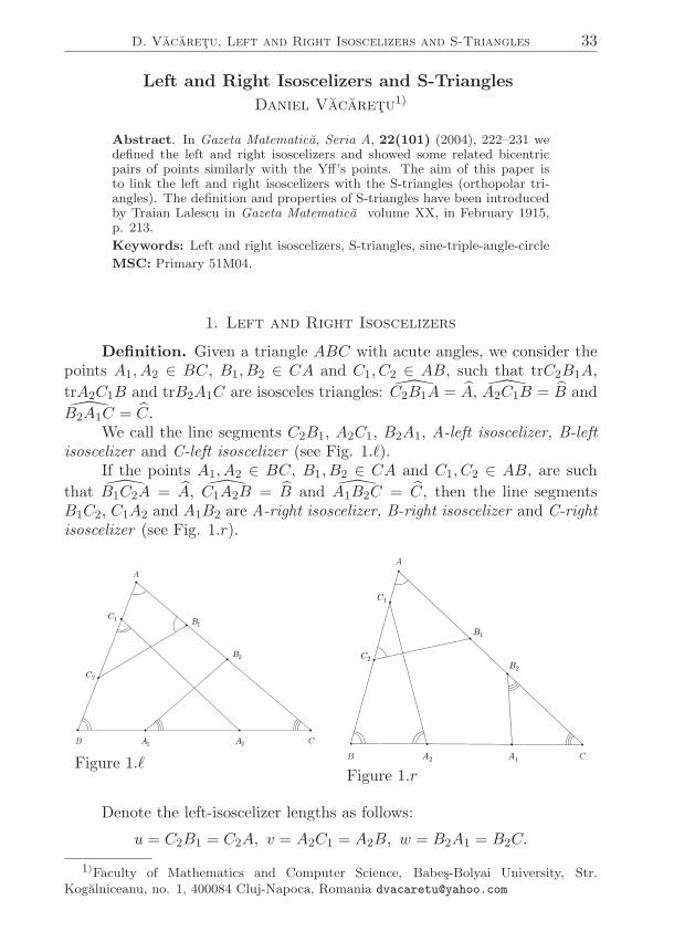
Definition. Given a triangle ABC with acute angles, we consider thepoints A1, A2 ∈ BC, B1, B2 ∈ CA and C1, C2 ∈ AB, such that trC2B1A,
trA2C1B and trB2A1C are isosceles triangles: C2B1A = A, A2C1B = B and
B2A1C = C.We call the line segments C2B1, A2C1, B2A1, A-left isoscelizer, B-left
isoscelizer and C-left isoscelizer (see Fig. 1.ℓ).If the points A1, A2 ∈ BC, B1, B2 ∈ CA and C1, C2 ∈ AB, are such
that B1C2A = A, C1A2B = B and A1B2C = C, then the line segmentsB1C2, C1A2 and A1B2 are A-right isoscelizer, B-right isoscelizer and C-rightisoscelizer (see Fig. 1.r).
1A 2
A
1B
2B
1C
2C
A
B C
Figure 1.ℓ 1A
2A
1B
2B
1C
2C
A
B C
Figure 1.r
Denote the left-isoscelizer lengths as follows:
u = C2B1 = C2A, v = A2C1 = A2B, w = B2A1 = B2C.
1)Faculty of Mathematics and Computer Science, Babes-Bolyai University, Str.Kogalniceanu, no. 1, 400084 Cluj-Napoca, Romania [email protected]
34 Articole
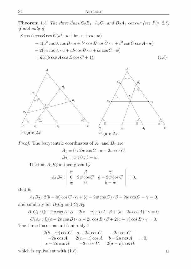
Theorem 1.ℓ. The three lines C2B1, A2C1 and B2A1 concur (see Fig. 2.ℓ)if and only if
8 cosA cosB cosC(ab · u+ bc · v + ca · w)− 4(a2 cosA cosB · u+ b2 cosB cosC · v + c2 cosC cosA · w)+ 2(ca cosA · u+ ab cosB · v + bc cosC · w)= abc(8 cosA cosB cosC + 1). (1.ℓ)
1A
2A
1B
2B
1C
2C
1I
A
B C
Figure 2.ℓ1
A2
A
1B
2B1
C
2C
I
A
B C
r
Figure 2.r
Proof. The barycentric coordinates of A1 and B2 are:
A1 = 0 : 2w cosC : a− 2w cosC,
B2 = w : 0 : b− w.
The line A1B2 is then given by
A1B2 :
∣∣∣∣∣∣
α β γ
0 2w cosC a− 2w cosCw 0 b− w
∣∣∣∣∣∣= 0,
that is
A1B2 : 2(b− w) cosC · α+ (a− 2w cosC) · β − 2w cosC − γ = 0,
and similarly for B1C2 and C1A2:
B1C2 : Q− 2u cosA · α+ 2(c− u) cosA · β + (b− 2u cosA) · γ = 0,
C1A2 : Q(c− 2v cosB) · α− 2v cosB · β + 2(a− v) cosB · γ = 0.
The three lines concur if and only if∣∣∣∣∣∣
2(b− w) cosC a− 2w cosC −2w cosC−2u cosA 2(c− u) cosA b− 2u cosAc− 2v cosB −2v cosB 2(a− v) cosB
∣∣∣∣∣∣= 0,
which is equivalent with (1.ℓ). 2
D. Vacaretu, Left and Right Isoscelizers and S-Triangles 35
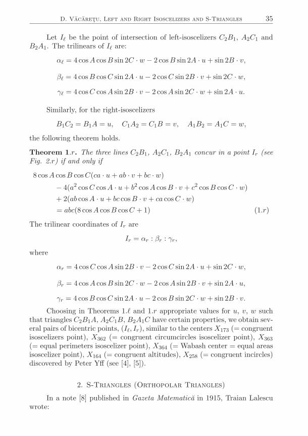
Let Iℓ be the point of intersection of left-isoscelizers C2B1, A2C1 andB2A1. The trilinears of Iℓ are:
αℓ = 4 cosA cosB sin 2C · w − 2 cosB sin 2A · u+ sin 2B · v,
βℓ = 4 cosB cosC sin 2A · u− 2 cosC sin 2B · v + sin 2C · w,
γℓ = 4 cosC cosA sin 2B · v − 2 cosA sin 2C · w + sin 2A · u.
Similarly, for the right-isoscelizers
B1C2 = B1A = u, C1A2 = C1B = v, A1B2 = A1C = w,
the following theorem holds.
Theorem 1.r. The three lines C2B1, A2C1, B2A1 concur in a point Ir (seeFig. 2.r) if and only if
8 cosA cosB cosC(ca · u+ ab · v + bc · w)− 4(a2 cosC cosA · u+ b2 cosA cosB · v + c2 cosB cosC · w)+ 2(ab cosA · u+ bc cosB · v + ca cosC · w)= abc(8 cosA cosB cosC + 1) (1.r)
The trilinear coordinates of Ir are
Ir = αr : βr : γr,
where
αr = 4 cosC cosA sin 2B · v − 2 cosC sin 2A · u+ sin 2C · w,
βr = 4 cosA cosB sin 2C · w − 2 cosA sin 2B · v + sin 2A · u,
γr = 4 cosB cosC sin 2A · u− 2 cosB sin 2C · w + sin 2B · v.Choosing in Theorems 1.ℓ and 1.r appropriate values for u, v, w such
that triangles C2B1A, A2C1B, B2A1C have certain properties, we obtain sev-eral pairs of bicentric points, (Iℓ, Ir), similar to the centers X173 (= congruentisoscelizers point), X362 (= congruent circumcircles isoscelizer point), X363
(= equal perimeters isoscelizer point), X364 (= Wabash center = equal areasisoscelizer point), X164 (= congruent altitudes), X258 (= congruent incircles)discovered by Peter Yff (see [4], [5]).
2. S-Triangles (Orthopolar Triangles)
In a note [8] published in Gazeta Matematica in 1915, Traian Lalescuwrote:
36 Articole
“Given a triangle ABC and two points B′ and C ′ on its cir-cumcircle. Let A′ be the point on the same circle for whichthe Simson line is perpendicular on B′C ′. It is known thatthis point is obtained as follows:
From A we draw a straight line perpendicular on B′C ′
which intersect the circle in A′′ and from A′′ we draw thestraight line perpendicular on BC which intersect the circlein the searched point A′. We say that the triangle A′B′C ′ isa S-triangle with respect to the triangle ABC.”
Next, Traian Lalescu proved the following properties:
1) The algebraic sum of arcs
AA′,
BB′ and
CC ′ considered with thesame orientation is zero:
m(
AA′) + m(
BB′) + m(
CC ′) ≡ 0 (mod 2π).
2) The Simson line of each vertex of the triangle A′B′C ′ is perpendicularon the opposite side of this triangle.
3) The Simson lines of A′, B′, C ′ with respect to triangle ABC areconcurrent.
4) The triangleABC is an S-triangle with respect to the triangleA′B′C ′.5) The intersection point of the six Simson lines is the midpoint of the
line segment joining the orthocenters of triangles ABC and A′B′C ′ (see [8],[9], [10]).
Other authors showed that the point of intersection of the six Simsonlines is the common orthopole of each side of the triangle A′B′C ′ with respectto the triangle ABC and of each side of the triangle ABC with respect to thetriangle A′B′C ′, and for this reason the S-triangles are also named orthopolartriangles.
A classical example of S-triangles is the pair formed by the orthic trian-gle and the medial triangle, inscribed in the nine-point circle. The commonorthopole is the midpoint of the line segment joining X3 and X52, which isX389, the center of the Taylor’s circle = the Spiecker point (incenter of themedial triangle) of the orthic triangle (notations from [5]).
A natural generalization of the S-triangles is obtained by replacing theWallace-Simson lines with the Carnot lines.
Theorem 2.1. (Carnot) Given a triangle ABC and M a point on its cir-cumcircle. Let P ∈ BC, Q ∈ CA and R ∈ AB such that
m(MP,BC) = m(MQ,CA) = m(MR,AB) = ϕ.
Then the points P , Q and R are collinear, and the straight line PQR is calledthe ϕ-Carnot line.
D. Vacaretu, Left and Right Isoscelizers and S-Triangles 37
Definition 2.2. Given the triangle ABC, let B′ and C ′ two points on itscircumcircle and let A′ be the point on the same circle such that
m( ∆A′ , B′C ′) = π − ϕ,
where ∆A′ is the ϕ-Carnot line of the point A′ with respect to the triangleABC. We say that the triangle A′B′C ′ is a ϕ-S-triangle with respect totriangle ABC.
The point A′ is obtained by the following construction: From A we
draw the straight line AA′′ such that m( AA′′, B′C ′) = π − ϕ, where A′′ lieson the circumcircle of ABC, and from A′′ we draw the straight line A′′A′
such that m( A′′A′, BC) = ϕ, where A′ lies on the same circle. This point A′
is the searched point.
Theorem 2.3. The pair of triangles ABC and A′B′C ′ has the followingproperties:
1) m(
AA′) + m(
BB′) + m(
CC ′) ≡ 4ϕ (mod 2π). (2.1)2) The measure of the angle between the ϕ-Carnot line of each vertex
of the triangle A′B′C ′ with the opposite side of this triangle is π − ϕ.3) The ϕ-Carnot lines of A′, B′ and C ′ with respect to the triangle ABC
concur in a point Iϕ.4) The triangle ABC is a (π−ϕ)-S-triangle with respect to the triangle
A′B′C ′.5) The (π − ϕ)-Carnot lines of A, B and C with respect to the triangle
A′B′C ′ concur in the same point Iϕ ([3]).
Remarks. 1) The point Iϕ is the ϕ-isopole of each side of the triangle A′B′C ′
with respect to the triangle ABC and the (π−ϕ)-isopole of each side of thetriangle ABC with respect to the triangle A′B′C ′.
2) From m(
AA′) +m(
BB′) +m(
CC ′) ≡ 4ϕ (mod 2π) we may say thatevery pair of triangles inscribed in the same circle are in relationship (ϕ−S)and (π − ϕ) − S each with respect to the other. Actually, there are two
values ϕ1 and ϕ2 of ϕ ∈ (0, π), with |ϕ1 − ϕ2| =π
2, such that the relation
(2.1) holds.
A connection between the left and right isoscelizers and S-triangles isgiven by the following theorem.
Theorem 2.4. ([2]) Given the acute triangle ABC such that m(B) 6=1
2m(A) 6= m(C), m(C) 6= 1
2m(B) 6= m(A) and m(A) 6= 1
2m(C) 6= m(B).
Let Aℓ, Ar ∈ BC, Bℓ, Br ∈ CA and Cℓ, Cr ∈ AB such that BℓCℓ, CℓAℓ
and AℓBℓ are A-, B- and C-left isoscelizers and BrCr, CrAr and ArBr are
38 Articole
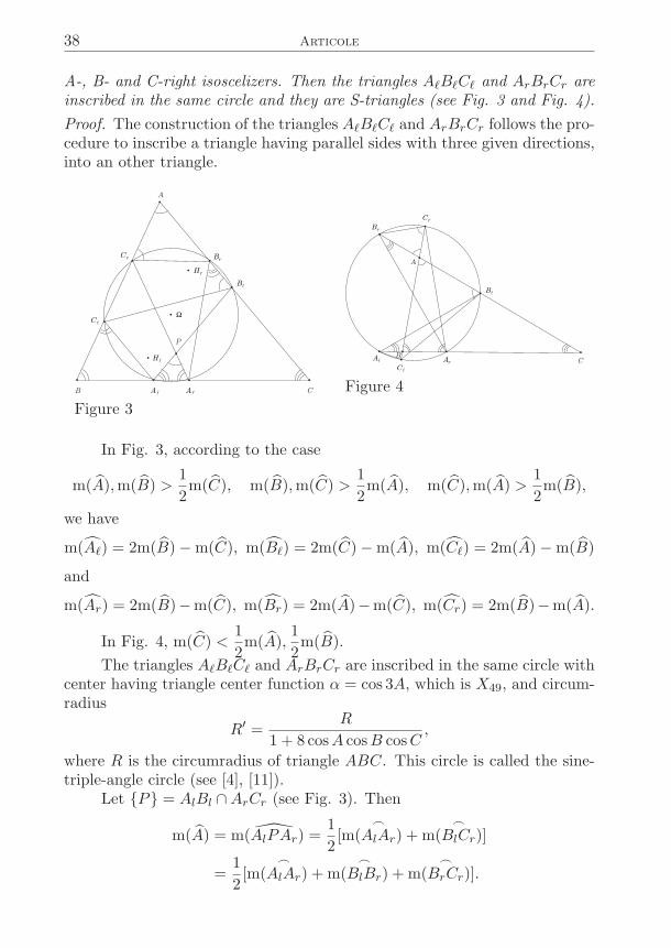
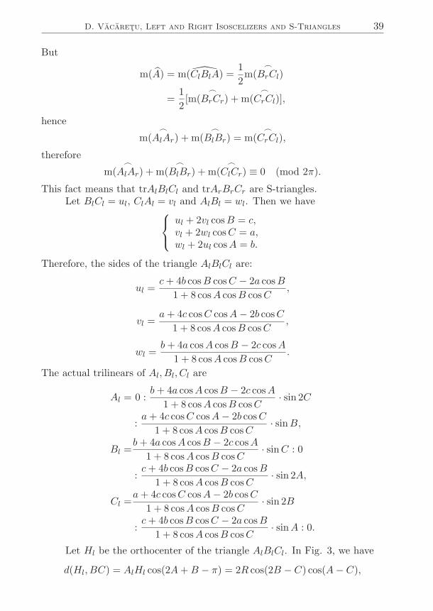
A-, B- and C-right isoscelizers. Then the triangles AℓBℓCℓ and ArBrCr areinscribed in the same circle and they are S-triangles (see Fig. 3 and Fig. 4).
Proof. The construction of the triangles AℓBℓCℓ and ArBrCr follows the pro-cedure to inscribe a triangle having parallel sides with three given directions,into an other triangle.
rAl A
rB
lB
rC
lC
rH
lH
W
A
B C
P
Figure 3
rAlA
rB
lB
rC
lC
A
BC
Figure 4
In Fig. 3, according to the case
m(A),m(B) >1
2m(C), m(B),m(C) >
1
2m(A), m(C),m(A) >
1
2m(B),
we have
m(Aℓ) = 2m(B)−m(C), m(Bℓ) = 2m(C)−m(A), m(Cℓ) = 2m(A)−m(B)
and
m(Ar) = 2m(B)−m(C), m(Br) = 2m(A)−m(C), m(Cr) = 2m(B)−m(A).
In Fig. 4, m(C) <1
2m(A),
1
2m(B).
The triangles AℓBℓCℓ and ArBrCr are inscribed in the same circle withcenter having triangle center function α = cos 3A, which is X49, and circum-radius
R′ =R
1 + 8 cosA cosB cosC,
where R is the circumradius of triangle ABC. This circle is called the sine-triple-angle circle (see [4], [11]).
Let P = AlBl ∩ArCr (see Fig. 3). Then
m(A) = m(AlPAr) =1
2[m(
AlAr) + m(
BlCr)]
=1
2[m(
AlAr) + m(
BlBr) + m(
BrCr)].
D. Vacaretu, Left and Right Isoscelizers and S-Triangles 39
But
m(A) = m(ClBlA) =1
2m(
BrCl)
=1
2[m(
BrCr) + m(
CrCl)],
hence
m(
AlAr) + m(
BlBr) = m(
CrCl),
therefore
m(
AlAr) + m(
BlBr) + m(
ClCr) ≡ 0 (mod 2π).
This fact means that trAlBlCl and trArBrCr are S-triangles.Let BlCl = ul, ClAl = vl and AlBl = wl. Then we have
ul + 2vl cosB = c,
vl + 2wl cosC = a,
wl + 2ul cosA = b.
Therefore, the sides of the triangle AlBlCl are:
ul =c+ 4b cosB cosC − 2a cosB
1 + 8 cosA cosB cosC,
vl =a+ 4c cosC cosA− 2b cosC
1 + 8 cosA cosB cosC,
wl =b+ 4a cosA cosB − 2c cosA
1 + 8 cosA cosB cosC.
The actual trilinears of Al, Bl, Cl are
Al = 0 :b+ 4a cosA cosB − 2c cosA
1 + 8 cosA cosB cosC· sin 2C
:a+ 4c cosC cosA− 2b cosC
1 + 8 cosA cosB cosC· sinB,
Bl =b+ 4a cosA cosB − 2c cosA
1 + 8 cosA cosB cosC· sinC : 0
:c+ 4b cosB cosC − 2a cosB
1 + 8 cosA cosB cosC· sin 2A,
Cl =a+ 4c cosC cosA− 2b cosC
1 + 8 cosA cosB cosC· sin 2B
:c+ 4b cosB cosC − 2a cosB
1 + 8 cosA cosB cosC· sinA : 0.
Let Hl be the orthocenter of the triangle AlBlCl. In Fig. 3, we have
d(Hl, BC) = AlHl cos(2A+B − π) = 2R cos(2B − C) cos(A− C),
40 Articole
where R is the radius of the cyclic hexagon AlArBlBrCrCl. Hence, thetrilinears of Hl are
Hl = cos(2B − C) cos(A− C) : cos(2C −A) cos(B −A)
: cos(2A−B) cos(C −B).
2
Remark. Hl is denoted P (61) in [7] and is named 1st Vacaretu Point.
Similarly, we have for the triangle ArBrCr
ur + 2wr cosC = b,
vr + 2ur cosA = c,
wr + 2vr cosB = a,
hence
ur =b+ 4c cosB cosC − 2a cosC
1 + 8 cosA cosB cosC,
vr =c+ 4a cosC cosA− 2b cosA
1 + 8 cosA cosB cosC,
wr =a+ 4b cosA cosB − 2c cosB
1 + 8 cosA cosB cosC.
The actual trilinears of Ar, Br, Cr are
Ar = 0 :a+ 4b cosA cosB − 2c cosB
1 + 8 cosA cosB cosC· sinC
:c+ 4a cosC cosA− 2b cosA
1 + 8 cosA cosB cosC· sin 2B,
Br =a+ 4b cosA cosB − 2c cosB
1 + 8 cosA cosB cosC· sin 2C : 0
:b+ 4c cosB cosC − 2a cosC
1 + 8 cosA cosB cosC· sinA,
Cr =c+ 4a cosC cosA− 2b cosA
1 + 8 cosA cosB cosC· sinB
:b+ 4c cosB cosC − 2a cosC
1 + 8 cosA cosB cosC· sin 2A : 0.
Let Hr be the orthocenter of the triangle ArBrCr. The trilinears of Hr
are
Hr = cos(2C −B) cos(A−B) : cos(2A− C) cos(B − C)
: cos(2B −A) cos(C −A).
The pair (Hl, Hr) is a pair of bicentric points (see [4], [5], [6]).The intersection point of the six Simson lines of Al, Bl, Cl with respect
to the triangle ArBrCr and of Ar, Br, Cr with respect to the triangle AlBlCl
D. Vacaretu, Left and Right Isoscelizers and S-Triangles 41
(= the common orthopole = the midpoint of the segment line HlHr = X1594,Rigby-Lalescu orthopole) is Hl ⊕Hr and its trilinears are
α = cos(2B − C) cos(A− C) + cos(2C −B) cos(A−B),
β = cos(2C −A) cos(B −A) + cos(2A− C) cos(B − C),
γ = cos(2A−B) cos(C −B) + cos(2B −A) cos(C −A).
From the sine law, we may compute the radius R of the circumcircle ofthe triangles AlBlCl, ArBrCr:
ul
sin(2B − C)=
vl
sin(2C −A)=
wl
sin(2A−B)=
ur
sin(2C −B)
=vr
sin(2A− C)=
wr
sin(2B −A)= 2R.
Finally, let Ω be the center of the circumcircle of the triangles AlBlCl
and ArBrCr. We have
m(ΩArCr) =1
2π − 2[2m(A)−m(C)]
=π
2− 2m(A) + m(C).
Therefore
m(ΩArCr) = m(ΩArCr) + m(CrArB)
=π
2− 2m(A) + m(C) + m(B)
=3π
2− 3m(A).
Hence
d(Ω, BC) = R sin
[3π
2− 3m(A)
]= −R cos(3A).
Therefore the trilinears of Ω are
Ω = cos(3A) : cos(3B) : cos(3C),
hence Ω = X49 = center of sine-triple-angle-circle ([4], [5]).
References
[1] R. Honsberger, Episodes in Nineteenth and Twentieth Century Euclidean Geometry,Mathematical Association of America, 1995.
[2] A. Jurjut and D. Vacaretu, Problem C:105 (An Example of S-Triangles) (in Roma-nian), Gazeta Matematica, 87 (1982), nr. 7, 246–248.
[3] A. Jurjut and D. Vacaretu, A generalization of S-Triangles (in Romanian), Gazeta
Matematica, 87 (1982), nr. 8, 296–300.[4] C. Kimberling, Triangle Centers and Central Triangles, Congressus Numerantius, 129
(1998), 1–295.[5] C. Kimberling, Encyclopedia of Triangle Centers, 05.03.2016 edition, available at
http://faculty.evansville.edu.ck6/encyclopedia/ETC.html
42 Articole
[6] C. Kimberling, Bicentric Pairs of Points and Related Triangle Centers, Forum Geom.
3 (2003), 35–47.[7] C. Kimberling, faculty.evansville.edu/ck6/encyclopedia/BicentricPairs.html[8] T. Lalescu, A class of remarkable triangles (in Romanian), Gazeta Matematica, 20
(1915), 213.[9] T. Lalesco, La Geometrie du Triangle, Paris, Librairie Vuibert, 1937.
[10] C. Mihalescu, The Geometry of Remarkable Elements (in Romanian), Ed. Tehnica,Bucharest, 1957.
[11] V. Thebault, Sine-Triple-Angle-Circle, Mathesis 65 (1956), 282–284.[12] D. Vacaretu, Left and right isoscelizers and some related bicentric pairs of points,
Gazeta Matematica, Seria A, 22(101) (2004), 222–231.
S. K. Jena, On a new family of semi-perfect cuboids 43
NOTE MATEMATICE
On a new family of semi-perfect cuboids
Susil Kumar Jena1)
Abstract. In this paper, we give a new parametric solution of one of thethree variations of one classical open problem relating to the perfect cuboid.With this solution, one can find infinitely many semi-perfect cuboids eachof which has integer sides such that two face diagonals and the body diag-onal are of integral lengths.
Keywords: Rational cuboids, Diophantine equations, perfect cuboids,semi-perfect cuboids.
MSC: Primary 11D41; Secondary 11D72.
Introduction
The question whether there can be a perfect rational cuboid, which is arectangular parallelepiped whose three edges, three face diagonals and bodydiagonal all have integer lengths, is yet to be answered. If a, b, c representthe lengths of the edges; p, q, r, the face diagonals; and d, the body diagonal,what is sought is a solution to the following system of equations:
a2 + b2 = p2;
a2 + c2 = q2; (1)
b2 + c2 = r2;
a2 + b2 + c2 = d2,
where a, b, c, p, q, r and d are positive integers. Here, we have to find sevenrelated integer quantities: the lengths of three edges, three face diagonals,and the body diagonal. Till May, 2016, we do not have the solution for thesystem of Diophantine equations (1). But, if we ask for only six of these tobe integers, then there are three variations of this problem as follows:
I. The body diagonal does not have integer length.II. One of the face diagonals does not have integer length.III. One of the edges does not have integer length.
The rational cuboids falling into any one of these three variations are calledsemi-perfect cuboids. Infinitely many solutions do exist for all the three varia-tions, though none of them is complete (see [2] and [9]). Many papers dealingwith different aspects of this problem are published (see [1], [3], [4], [7], [8],[10]–[13]). The historical details of this problem can be found in [5], and forother related research one may refer [6].
1)(Former Professor of Electronics & Telecommunication Engineering), Plot No-170, Sector-5, Niladri Vihar, Chandrasekharpur, Bhubaneswar-751021, Odisha, India,susil [email protected]
44 Note Matematice
In this paper, we give a new parametric solution for the semi-perfectcuboids of Variation III followed by a table containing some numerical results.Here, our approach is purely elementary.
1. The Problem and the solution
For given positive integers a, b, c, d, p, q, we want to find the primitiveand non-trivial solutions of the following system of Diophantine equations:
a2 + b2 = p2;
a2 + c2 = q2; (2)
and
a2 + b2 + c2 = d2.
In (2), take
a = 2√xyzt , b = xy − zt , c = xz − yt. (3)
So, we get
p2 = a2 + b2 = (2√xyzt)2 + (xy − zt)2 = (xy + zt)2;
q2 = a2 + c2 = (2√xyzt)2 + (xz − yt)2 = (xz + yt)2; (4)
d2 = a2 + b2 + c2 = (2√xyzt)2 + (xy − zt)2 + (xz − yt)2
= x2y2 + z2t2 + x2z2 + y2t2 = (y2 + z2)(x2 + t2).
Thus, from (4) we have
p = (xy + zt);
q = (xz + yt); (5)
d =√(y2 + z2)(x2 + t2).
Taking x = α2 − β2, y = m2 − n2, z = 2mn, and t = 2αβ in (3) and (5), andrearranging, we get
a = 4√mnαβ(m2 − n2)(α2 − β2);
b = (m2 − n2)(α2 − β2)− 4mnαβ;
c = 2mn(α2 − β2)− 2αβ(m2 − n2);
p = (m2 − n2)(α2 − β2) + 4mnαβ; (6)
q = 2mn(α2 − β2) + 2αβ(m2 − n2);
d =√(m2 + n2)2(α2 + β2)2
= (m2 + n2)(α2 + β2).
We state a lemma which will be used to modify (6) after appropriate substi-tutions to suit our requirement.
S. K. Jena, On a new family of semi-perfect cuboids 45
Lemma 1. For any non-zero integers m,n, α, β, if α = (m2−n2+2mn)2 andβ = (m2−n2−2mn)2, then, αβ = (m4−6m2n2+n4)2, α2−β2 = 16mn(m2−n2)(m2 + n2)2 and α2 + β2 = 2(m8 + 20m6n2 − 26m4n4 + 20m2n6 + n8).
Proof. The proof is too elementary, and can be easily verified. 2
In (6), substituting the values of α, β, αβ, (α2−β2) and (α2+β2) fromLemma 1, and then, scaling down the calculated expressions for a, b, c, p, q,d by their common factor 2, we get
a = 8mn(m8 − 6m6n2 + 6m2n6 − n8);
b = 2mn(3m8 + 12m6n2 − 46m4n4 + 12m2n6 + 3n8);
c = (m2 − n2)(−m8 + 28m6n2 − 6m4n4 + 28m2n6 − n8); (7)
p = 2mn(5m8 − 12m6n2 + 30m4n4 − 12m2n6 + 5n8);
q = (m2 − n2)(m8 + 4m6n2 + 70m4n4 + 4m2n6 + n8);
d = (m2 + n2)(m8 + 20m6n2 − 26m4n4 + 20m2n6 + n8).
If we take r2 = b2 + c2, then based on (7) we calculate
r = (m20 − 22m18n2 + 1197m16n4 − 2568m14n6 − 942m12n8 (8)
+ 5692m10n10 − 942m8n12 − 2568m6n14 + 1197m4n16
− 22m2n18 + n20)1/2.
2. Some numerical solutions
In the following table we give the absolute value of numerical solu-tions to (2) by using (7) in the range 2 ≤ m ≤ 10 and 1 ≤ n ≤ 10 wheregcd(m,n) = 1. In (7), inter-changing m ↔ n does not affect the absolutevalues of the functions involved. So, in the calculation table we take onlyone pair of values for (m,n) instead of two pairs which are obtained by inter-changing the values of m and n. When both m and n are odd, we get 32 asa common factor in the calculated values of (a, b, c, p, q, d). In this case, wehave to pass over this factor to get primitive solutions for (a, b, c, p, q, d). Inall these numerical solutions as given in the table, we calculated the values ofr to be irrational in accordance with (8). Now, there are two options: eitherwe prove that for any integer pair (m,n), r is never an integer; or, we maylike to search extensively to find an (m,n) pair for which r is a positive inte-ger. If one is lucky enough with the second option, the search for a perfectcuboid will be over.
References
[1] A. Bremner, The rational cuboid and a quartic surface, Rocky Mountain J. Math.
18(1988), 105–121.[2] W. J. A. Colman, On certain semi-perfect cuboids, Fibonacci Quart. 26 (1988), 54–57.
46 Note Matematice
[3] W. J. A. Colman, Some Observations on the Classical Cuboid and Its ParametricSolutions, Fibonacci Quart. 26 (1988), 338–343.
[4] W. J. A. Colman, A perfect cuboid in Gaussian integers, Fibonacci Quart. 32 (1994),266–268.
[5] L. E. Dickson, History of the Theory of Numbers, Vol. 2, Diophantine Analysis, Wash-ington, 1920: ch 15, ref. 28, p. 448 and cross-refs. to pp. 446–458; ch. 19, refs 1–30,40–45, pp. 497–502, 505–507.
[6] R. K. Guy, Unsolved Problems in Number Theory, Third Edition, Springer Sci-ence+Business Media, Inc., New York, 2004. pp. 275–283.
[7] I. Korec, Nonexistence of a small perfect rational cuboid, I., II., Acta Math. Univ.
Comenian. 42/43(1983), 73–86, 44/45(1984) 39–48.[8] I. Korec, Lower bounds for perfect rational cuboids, Math. Slovaka 42(1992), 565–582.[9] J. Leech, The Rational Cuboid Revisited, Amer. Math. Monthly 84(7)(1977), 518–533;
corrections (Jean Lagrange) 85(1978).[10] J. Leech, Five tables related to rational cuboids, Math. Comput. 32(1978), 657–659.[11] J. Leech, A remark on rational cuboids, Canad. Math. Bull. 24(1981), 377–378.[12] N. Narumiya, H. Shiga, On Certain Rational Cuboid Problems, Nihonkai Math. J.
Volume 12, 1(2001), 75–88.[13] T. Roberts, Some constraints on the existence of a perfect cuboid, Australian Mathe-
matical Society Gazette 37(2010), 29–31.
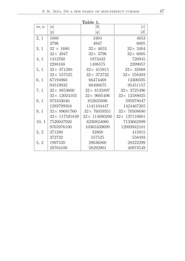
S. K. Jena, On a new family of semi-perfect cuboids 47
Table 1.m,n |a| |b| |c|
|p| |q| |d|2, 1 1680 3404 4653
3796 4947 60053, 1 32 × 1680 32× 4653 32× 3404
32× 4947 32× 3796 32× 60054, 1 1313760 1873432 720945
2288168 1498575 23990575, 1 32× 371280 32× 415915 32× 32868
32× 557525 32× 372732 32× 5584936, 1 67194960 66474468 13300595
94519932 68498675 954511577, 1 32× 8853600 32× 8135897 32× 3725496
32× 12024103 32× 9605496 32× 125880258, 1 973103040 852635696 595978047
1293799504 1141104447 14244672659, 1 32× 89681760 32× 76059351 32× 70508680
32× 117591849 32× 114080200 32× 13711060110, 1 7520047920 6230824060 7133662899
9765976100 10365339699 120939421013, 2 371280 32868 415915
372732 557525 5584935, 2 1997520 29636860 28222299
29704100 28292901 40973549
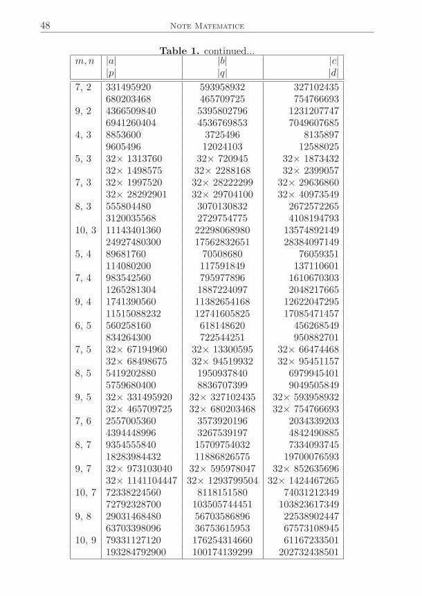
48 Note Matematice
Table 1. continued...m,n |a| |b| |c|
|p| |q| |d|7, 2 331495920 593958932 327102435
680203468 465709725 7547666939, 2 4366509840 5395802796 1231207747
6941260404 4536769853 70496076854, 3 8853600 3725496 8135897
9605496 12024103 125880255, 3 32× 1313760 32× 720945 32× 1873432
32× 1498575 32× 2288168 32× 23990577, 3 32× 1997520 32× 28222299 32× 29636860
32× 28292901 32× 29704100 32× 409735498, 3 555804480 3070130832 2672572265
3120035568 2729754775 410819479310, 3 11143401360 22298068980 13574892149
24927480300 17562832651 283840971495, 4 89681760 70508680 76059351
114080200 117591849 1371106017, 4 983542560 795977896 1610670303
1265281304 1887224097 20482176659, 4 1741390560 11382654168 12622047295
11515088232 12741605825 170854714576, 5 560258160 618148620 456268549
834264300 722544251 9508827017, 5 32× 67194960 32× 13300595 32× 66474468
32× 68498675 32× 94519932 32× 954511578, 5 5419202880 1950937840 6979945401
5759680400 8836707399 90495058499, 5 32× 331495920 32× 327102435 32× 593958932
32× 465709725 32× 680203468 32× 7547666937, 6 2557005360 3573920196 2034339203
4394448996 3267539197 48424908858, 7 9354555840 15709754032 7334093745
18283984432 11886826575 197000765939, 7 32× 973103040 32× 595978047 32× 852635696
32× 1141104447 32× 1293799504 32× 142446726510, 7 72338224560 8118151580 74031212349
72792328700 103505744451 1038236173499, 8 29031468480 56703586896 22538902447
63703398096 36753615953 6757310894510, 9 79331127120 176254314660 61167233501
193284792900 100174139299 202732438501


![[The Stute] October 16, 2015 (Issue 7, Volume CXIII)](https://img.pdfslide.us/doc/110x75/5790700c1a28ab68749bad7a/the-stute-october-16-2015-issue-7-volume-cxiii.jpg)


![[The Stute] April 22, 2016 (Issue 25, Volume CXIII)](https://img.pdfslide.us/doc/110x75/579077aa1a28ab6874bece54/the-stute-april-22-2016-issue-25-volume-cxiii.jpg)


![[The Stute] September 18, 2015 (Issue 3, Volume CXIII](https://img.pdfslide.us/doc/110x75/57906edc1a28ab687496328c/the-stute-september-18-2015-issue-3-volume-cxiii.jpg)