GazeMAE: General Representations of EyeMovements using a Micro-Macro Autoencoder

Louise Gillian C. BautistaDepartment of Computer Science

University of the PhilippinesEmail: lcbautista1@up.edu.ph

Prospero C. Naval, Jr.Department of Computer Science

University of the PhilippinesEmail: pcnaval@up.edu.ph

Abstract—Eye movements are intricate and dynamic eventsthat contain a wealth of information about the subject and thestimuli. We propose an abstract representation of eye movementsthat preserve the important nuances in gaze behavior while beingstimuli-agnostic. We consider eye movements as raw position andvelocity signals and train separate deep temporal convolutionalautoencoders. The autoencoders learn micro-scale and macro-scale representations that correspond to the fast and slow featuresof eye movements. We evaluate the joint representations witha linear classifier fitted on various classification tasks. Ourwork accurately discriminates between gender and age groupsand outperforms previous works on biometrics and stimuliclassification. Further experiments highlight the validity andgeneralizability of this method, bringing eye-tracking researchcloser to real-world applications.

I. INTRODUCTION

Our eyes move in response to top-down and bottom-up fac-tors, subconsciously influenced by a stimuli’s characteristicsand our own goals [1]. Eye movements can be seen simply asa sequence of fixations and saccades: at some points we keepour eyes still to take in information, then rapidly move themto switch our point of focus. Thus, eye movements tell a lotabout our perception, thought, and decision-making processes[2]. In addition, there exist less-pronounced eye movementseven within a fixation, among them are microsaccades thathave recently been found to have numerous links to attention,memory, and cognitive load [3], [4], [5], [6]. Overall, suchfindings encourage eye-tracking technology to be brought tovarious fields such as human-computer interaction, psychol-ogy, education, medicine, and security [7].

Bridging the gap between laboratory findings and real-worldapplications require that eye movements are processed usingrepresentations or feature vectors as inputs to algorithms.Common methods to do so include processing gaze intoparameters [8] (e.g. fixation counts and durations), maps [9](e.g. heat maps, saliency maps), scanpaths [10] (e.g. stringsequences), and graphical models [11], [12] that considerimage regions as nodes and saccades as edges.

However, these methods have two main drawbacks thatinhibit them from optimally representing eye movements.First, they do not exploit the wealth of information present ineye movements. By discretizing movements into fixations andsaccades, they flatten the dynamic nature of eye movementsand lose the tiny but important nuances. Additionally, event

detection is still an active research area and as such may beprone to inaccuracies and inconsistencies [13], [14]. Second,they are not generalizable due to the tight links of the methodsto the stimuli, thereby limiting eye movement comparison tothose elicited from the same image or stimuli. Scanpaths andgraphs additionally have a dependence on pre-defined areas ofinterest (AoIs). This may be mitigated by learning AoIs in adata-driven manner, but this in turn introduces dependencieson the method and on the amount and quality of data availablefor each new stimulus.

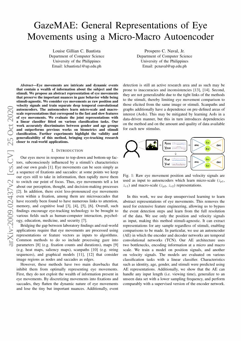
Fig. 1: Raw eye movement position and velocity signals areused as input to autoencoders which learn micro-scale (zp1,zv1) and macro-scale (zp2, zv2) representations.

In this work, we use deep unsupervised learning to learnabstract representations of eye movements. This removes theneed for extensive feature engineering, allowing us to bypassthe event detection steps and learn from the full resolutionof the data. We use only the position and velocity signalsas input, making this method stimuli-agnostic. It can extractrepresentations for any sample regardless of stimuli, enablingcomparisons to be made. In particular, we use an autoencoder(AE) in which the encoder and decoder networks are temporalconvolutional networks (TCN). Our AE architecture usestwo bottlenecks, encoding information at a micro and macroscale. We train a model on position signals, and anotheron velocity signals. The models are evaluated on variousclassification tasks with a linear classifier. Characteristicssuch as identity, age, gender, and stimuli were predicted usingAE representations. Additionally, we show that the AE canhandle any input length (i.e. viewing time), generalize to anunseen data set with a lower sampling frequency, and performcomparably with a supervised version of the encoder network.

arX

iv:2

009.

0243

7v2

[cs

.CV

] 2

5 O

ct 2

020

The contributions of this paper are as follows:

1) We apply deep unsupervised learning to eye movementsignals such that representations are learned withoutsupervision or feature engineering.

2) We learn representations for eye movements that arestimuli-agnostic.

3) We propose a modified autoencoder with two bottle-necks that learn fast and slow features of the eye move-ment signal. This autoencoder also uses an interpolativedecoder instead of a regular Temporal ConvolutionalNetwork or an autoregressive decoder.

4) We show that the representations learned are meaningful.They are able to accurately classify labels, generalize toan unseen data set, scale to long input lengths. Further-more, similar data points exhibit clustering properties.

Note that this work is limited to eye movements gathered onstatic and visual stimuli, recorded with research-grade eye-trackers. Eye movements on texts, videos, or ”in the wild” arebeyond our scope. Source code and models are available athttps://github.com/chipbautista/gazemae.

II. METHODOLOGY

A. Preliminaries

1) Representation Learning: The goal of representationlearning, also called feature learning, is to abstract informationfrom data such that the underlying factors of variation in thedata are captured [15]. This involves mapping an input to anembedding space which meaningfully describe the originaldata. A common use case for learning representations is toact as a preprocessing step for downstream tasks in which therepresentation, often notated as z of a data point x, will beused as the input for classifiers and predictors. Representationlearning methods are commonly unsupervised methods, whereno external labels about the data is required. Therefore, thesecan take advantage of any available data to learn more robustfeatures.

2) Autoencoder: An autoencoder (AE) is a neural networkthat learns a representation of an input data by attempting toreconstruct a close approximation of the input. A typical AEis undercomplete, i.e. it uses a bottleneck to compresses theinput to a lower-dimensional space before producing an outputwith the same dimensions as the input.

Generally, an AE works as follows: an encoder f(x) mapsthe original input x ∈ Rdx to a latent vector z ∈ Rdz , and adecoder g(z) maps z to an output x ∈ Rdx . It is trained toreconstruct x, i.e. x ≈ x.

Since dz < dx, the encoder is forced to learn only the rele-vant information such that the decoder g is able to sufficientlyreconstruct the original input. This is a simple framework tolearn a representation of the data, and is commonly thoughtof as a non-linear version of Principal Component Analysis(PCA) [15]. Because an AE uses the input data as its targetoutput, it is a self-supervised method for representation learn-ing.

3) Temporal Convolutional Network: The temporal convo-lutional network (TCN) [16] is a generic convolutional neuralnetwork (CNN) architecture that has recently been shown tooutperform Recurrent Neural Networks (RNNs). TCNs workin the same manner as the CNN, where each convolutionallayer convolves a number of 1-dimensional kernels (c filtersof size 1 × k) across the input data to recognize sequencepatterns [17]. A TCN modifies the convolution operation intothe following:

1) Dilated Convolutions, where the kernel skips d − 1values. For a learnable kernel K with kernel size k anddilation d, the output at a subsequence x of size n in aninput X is calculated with the following:

k∑i=0

Ki · xn−di

Dilations are commonly increased exponentially acrosslayers, e.g. 20, 21, 22, ...2l. This enables the output inlayer l to be calculated with higher receptive field i.e.from a wider input range.

2) Causal Convolutions The output at time t is calculatedusing only the values from the previous time steps t −1, t − 2, t − 3, .... This is done by padding d(k − 1)zeroes on the left of the input. In effect, this emulatesthe sequential processing of RNNs.

B. Data Sets

1) EMVIC: The Eye Movements Verification and Identifi-cation Competition (EMVIC) 2014 [18] is a data set used as abenchmark for Biometrics, where subjects are to be identifiedbased only on their eye movements. They collected datafrom 34 subjects who were shown a number of normalizedface images (the eyes, nose, and mouth are in roughly thesame position in the images). The viewing times spent bythe subjects to look at the face images range from 891 msto 22012 ms, and the average is 2429 ms or roughly 2.5seconds. Eye movements were recorded using a Jazz-Novoeye tracker with a 1000 Hz sampling frequency, i.e. it records1000 gaze points per second. 1,430 eye movement sampleswere collected, where the training set consists of 837 samplesfrom 34 subjects and the test set consists of 593 from 22subjects.

2) FIFA: The Fixations in Faces (FIFA) [19] is an eyemovement data set of 7 subjects using 250 images from indoorand outdoor scenes. Eye movements were recorded using SRResearch EyeLink 1000 eye-tracker with a 1000 Hz samplingfrequency. The images were of 1024x768 resolution and weredisplayed on a screen 80cm from the subject. This correspondsto a subjects’ visual angle of 28◦x 21◦. We obtain 3,200samples from this data set.

3) ETRA: The Eye Tracking Research & Applications(ETRA) data set was used to analyze saccades and microsac-cades in [3], [20] and was also used for a data miningchallenge in ETRA 2019. Eight subjects participated andviewed 4 image types: blank image, natural scenes, picture

puzzles, and ”Where’s Waldo?” images. For the blank andnatural image types, the subjects were free to view the imagein any manner. Picture puzzles contain two almost-identicalimages, and the subjects had to spot the differences betweenthe two. ”Where’s Waldo?” images are complex scenes filledwith small objects and characters, and the subjects had tofind the character Waldo. Each viewing was recorded for 45seconds.

Eye movements were recorded using an SR ResearchEyeLink II eye-tracker at 500 Hz sampling frequency. Thestimuli were presented such that they are within 36◦x 25.2◦ofthe subjects’ visual angle. 480 eye movement samples wereobtained from this data set.

Hz Stimuli Tasks Subj. Sample Time(s)

EMVIC 1000 face free 34 1430 ave.2.5s

FIFA 1000 natural free, 8 3200 2ssearch

ETRA 500 natural, free, 8 480 45spuzzle searchTotal 50 5110

TABLE I: Summary of data sets.

C. Data Preprocessing and Augmentation

To recap, we combine three data sets into a joint data setD. Each sample s ∈ R(2,t) is a vector with 2 channels (x andy) and a variable length t. To work across multiple data sets,we preprocess each s as follows:• We turn blinks (negative values) to zero since not all data

sets have blink data.• We standardize to a sampling frequency of 500 Hz. The

EMVIC and FIFA data sets are downsampled from 1000Hz to 500 Hz by dropping every other gaze point.

• We modify the coordinates such that the origin (0, 0) isat the top-left corner of the screen. This is to ensure thatthe network processes eye movements in the same scale.

• We scale the coordinates such that a subject’s 1◦of visualangle corresponds to roughly 35 pixels (1 dva ≈ 35px).For FIFA and ETRA data sets, these are estimated basedon their given eye-tracker and experiment specifications.For EMVIC, we leave the coordinates unprocessed dueto lack of details. This is done so that all movements areaccording to the same visual resolution of the subjects.

The inputs to the AEs are standardized into 2-secondsamples x ∈ R(2,t′), where t′ = 1000 = 500 Hz × 2s. Weincrease our data set by taking advantage of the ambiguity ofeye movements. For all 5,110 trials in the data sets, we take2-second time windows that slide forward in time by 20% or0.4s, which is equivalent to 200 gaze points. Each windowcounts as a new sample. With this, the training set size isincreased to 68,178 samples.

For all 5,110 trials in the data sets, we take 2s time windowsthat slide forward in time by 20% or 0.4s, which is equivalentto 200 gaze points. Using this method, the training set size isincreased to 68,178 samples.

Fig. 2: Top: a 2-second position signal at 500 Hz. Bottom: itscorresponding velocity signal.

D. Velocity Signals

In addition to the raw eye movement data given as a se-quence of positions across time (position signals (xpos, ypos)t),we also take the derivative, or the rate at which positionschange over time (velocity signals (xvel, yvel)t), simply calcu-lated as ( ∆x

ms ,∆yms ). We separately train a position autoencoder

(AEp) and velocity autoencoder (AEv) as they are expected tolearn different features. While position signals exhibit spatialinformation and visual saliency, velocity signals can revealmore behavioral information that may infer a subject’s thoughtprocess. Velocity is also commonly used as a threshold for eyemovement segmentation [13]. Figure 2 shows an example ofa position signal and a corresponding velocity signal. Positionsignals are further preprocessed by clipping the coordinates tothe maximum screen resolution: 1280x1024. For both signals,neither scaling nor mean normalization is done. Based on ourexperiments, we found that this was especially important forvelocity signals.

E. Network Architecture

In this subsection, we first describe the TCN architectureof both the encoder and decoder. Next, we describe how amicro and macro representations are learned in the bottlenecks.Lastly, we describe an interpolative decoder that fills in adestroyed signal to reconstruct or recover the original. Theoverall architecture of the autoencoder is visualized in Figure3, and a summary of its main components is shown in TableII. The number of filters and layers were chosen empirically.

position AE (AEp) velocity AE (AEv)Encoder TCN 128 filters x 8 layers 256 filters x 8 layersMicro-scale Bottleneck 64-dim FC 64-dim FCMacro-scale Bottleneck 64-dim FC 64-dim FC

Decoder TCN 128 filters x 4 layers; 128 x 8 layers64 filters x 4 layersTotal Parameters 652,228 1,964,676

TABLE II: Autoencoder specifications

1) Convolutional Layers: The encoder and decoder of theAE are implemented as TCNs. However, the encoder is non-causal in order to take in as much information as possible.

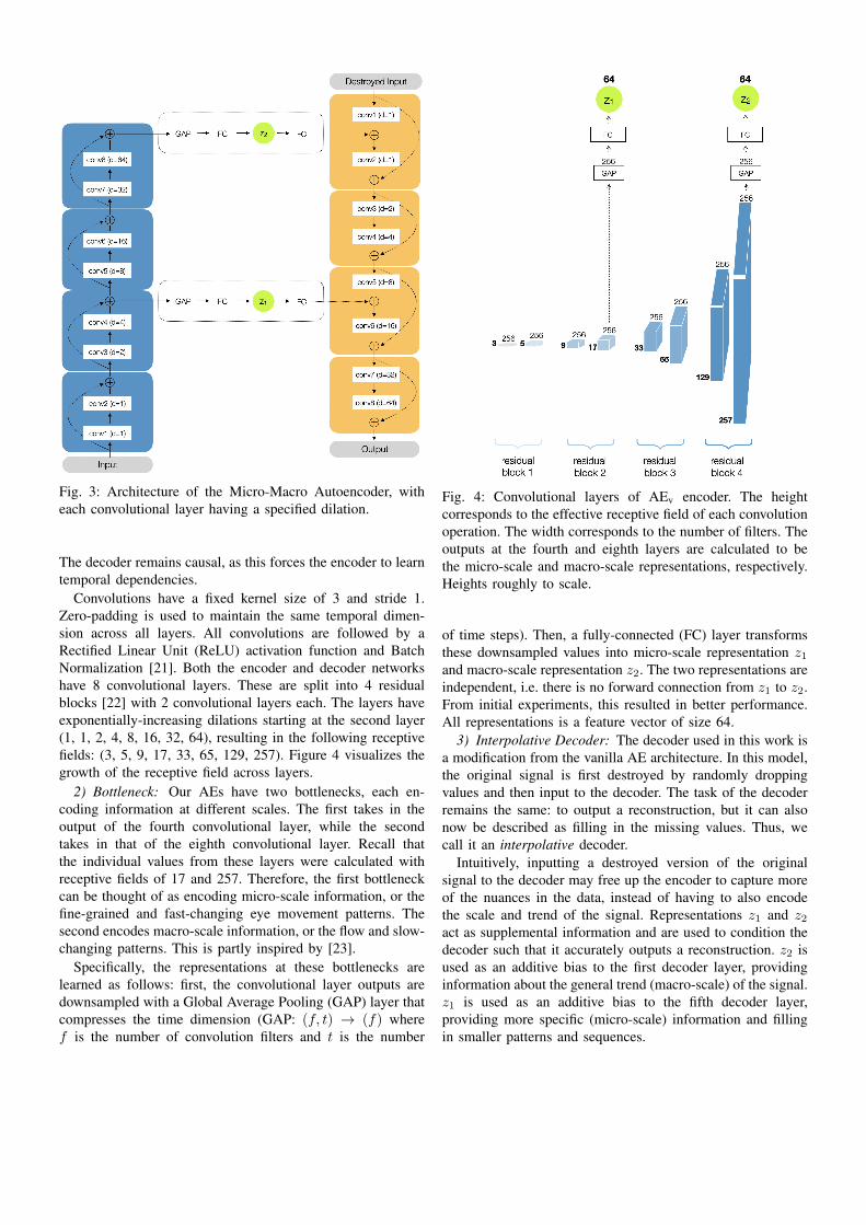
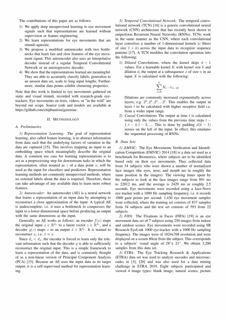
Fig. 3: Architecture of the Micro-Macro Autoencoder, witheach convolutional layer having a specified dilation.

The decoder remains causal, as this forces the encoder to learntemporal dependencies.

Convolutions have a fixed kernel size of 3 and stride 1.Zero-padding is used to maintain the same temporal dimen-sion across all layers. All convolutions are followed by aRectified Linear Unit (ReLU) activation function and BatchNormalization [21]. Both the encoder and decoder networkshave 8 convolutional layers. These are split into 4 residualblocks [22] with 2 convolutional layers each. The layers haveexponentially-increasing dilations starting at the second layer(1, 1, 2, 4, 8, 16, 32, 64), resulting in the following receptivefields: (3, 5, 9, 17, 33, 65, 129, 257). Figure 4 visualizes thegrowth of the receptive field across layers.

2) Bottleneck: Our AEs have two bottlenecks, each en-coding information at different scales. The first takes in theoutput of the fourth convolutional layer, while the secondtakes in that of the eighth convolutional layer. Recall thatthe individual values from these layers were calculated withreceptive fields of 17 and 257. Therefore, the first bottleneckcan be thought of as encoding micro-scale information, or thefine-grained and fast-changing eye movement patterns. Thesecond encodes macro-scale information, or the flow and slow-changing patterns. This is partly inspired by [23].

Specifically, the representations at these bottlenecks arelearned as follows: first, the convolutional layer outputs aredownsampled with a Global Average Pooling (GAP) layer thatcompresses the time dimension (GAP: (f, t) → (f) wheref is the number of convolution filters and t is the number

Fig. 4: Convolutional layers of AEv encoder. The heightcorresponds to the effective receptive field of each convolutionoperation. The width corresponds to the number of filters. Theoutputs at the fourth and eighth layers are calculated to bethe micro-scale and macro-scale representations, respectively.Heights roughly to scale.

of time steps). Then, a fully-connected (FC) layer transformsthese downsampled values into micro-scale representation z1

and macro-scale representation z2. The two representations areindependent, i.e. there is no forward connection from z1 to z2.From initial experiments, this resulted in better performance.All representations is a feature vector of size 64.

3) Interpolative Decoder: The decoder used in this work isa modification from the vanilla AE architecture. In this model,the original signal is first destroyed by randomly droppingvalues and then input to the decoder. The task of the decoderremains the same: to output a reconstruction, but it can alsonow be described as filling in the missing values. Thus, wecall it an interpolative decoder.

Intuitively, inputting a destroyed version of the originalsignal to the decoder may free up the encoder to capture moreof the nuances in the data, instead of having to also encodethe scale and trend of the signal. Representations z1 and z2

act as supplemental information and are used to condition thedecoder such that it accurately outputs a reconstruction. z2 isused as an additive bias to the first decoder layer, providinginformation about the general trend (macro-scale) of the signal.z1 is used as an additive bias to the fifth decoder layer,providing more specific (micro-scale) information and fillingin smaller patterns and sequences.

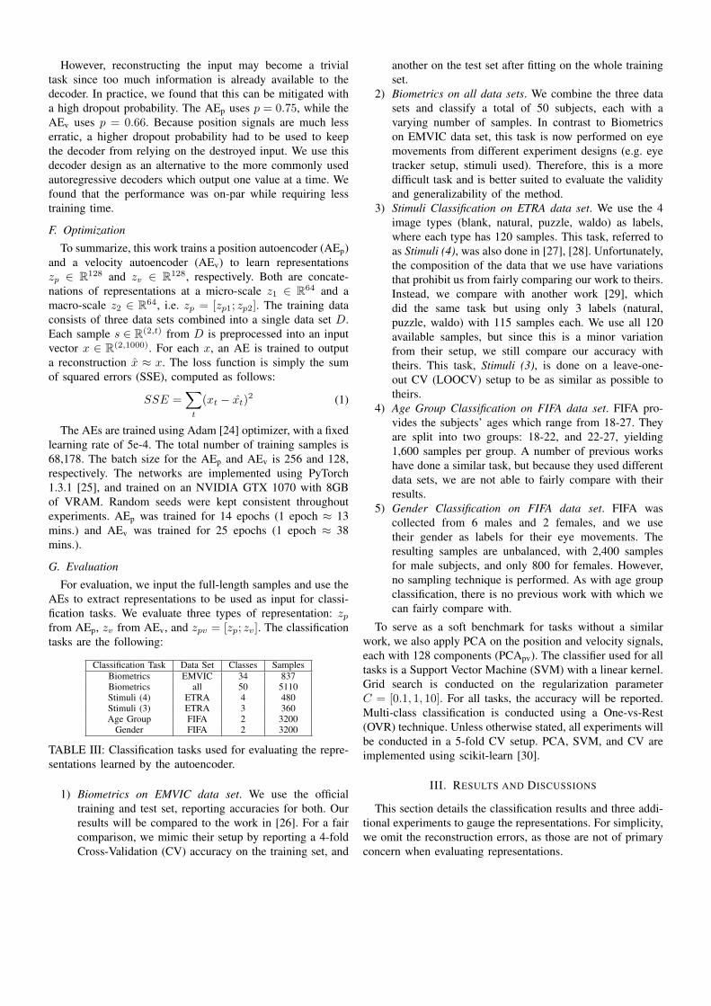
However, reconstructing the input may become a trivialtask since too much information is already available to thedecoder. In practice, we found that this can be mitigated witha high dropout probability. The AEp uses p = 0.75, while theAEv uses p = 0.66. Because position signals are much lesserratic, a higher dropout probability had to be used to keepthe decoder from relying on the destroyed input. We use thisdecoder design as an alternative to the more commonly usedautoregressive decoders which output one value at a time. Wefound that the performance was on-par while requiring lesstraining time.

F. Optimization

To summarize, this work trains a position autoencoder (AEp)and a velocity autoencoder (AEv) to learn representationszp ∈ R128 and zv ∈ R128, respectively. Both are concate-nations of representations at a micro-scale z1 ∈ R64 and amacro-scale z2 ∈ R64, i.e. zp = [zp1; zp2]. The training dataconsists of three data sets combined into a single data set D.Each sample s ∈ R(2,t) from D is preprocessed into an inputvector x ∈ R(2,1000). For each x, an AE is trained to outputa reconstruction x ≈ x. The loss function is simply the sumof squared errors (SSE), computed as follows:

SSE =∑t

(xt − xt)2 (1)

The AEs are trained using Adam [24] optimizer, with a fixedlearning rate of 5e-4. The total number of training samples is68,178. The batch size for the AEp and AEv is 256 and 128,respectively. The networks are implemented using PyTorch1.3.1 [25], and trained on an NVIDIA GTX 1070 with 8GBof VRAM. Random seeds were kept consistent throughoutexperiments. AEp was trained for 14 epochs (1 epoch ≈ 13mins.) and AEv was trained for 25 epochs (1 epoch ≈ 38mins.).

G. Evaluation

For evaluation, we input the full-length samples and use theAEs to extract representations to be used as input for classi-fication tasks. We evaluate three types of representation: zpfrom AEp, zv from AEv, and zpv = [zp; zv]. The classificationtasks are the following:

Classification Task Data Set Classes SamplesBiometrics EMVIC 34 837Biometrics all 50 5110Stimuli (4) ETRA 4 480Stimuli (3) ETRA 3 360Age Group FIFA 2 3200

Gender FIFA 2 3200

TABLE III: Classification tasks used for evaluating the repre-sentations learned by the autoencoder.

1) Biometrics on EMVIC data set. We use the officialtraining and test set, reporting accuracies for both. Ourresults will be compared to the work in [26]. For a faircomparison, we mimic their setup by reporting a 4-foldCross-Validation (CV) accuracy on the training set, and

another on the test set after fitting on the whole trainingset.

2) Biometrics on all data sets. We combine the three datasets and classify a total of 50 subjects, each with avarying number of samples. In contrast to Biometricson EMVIC data set, this task is now performed on eyemovements from different experiment designs (e.g. eyetracker setup, stimuli used). Therefore, this is a moredifficult task and is better suited to evaluate the validityand generalizability of the method.

3) Stimuli Classification on ETRA data set. We use the 4image types (blank, natural, puzzle, waldo) as labels,where each type has 120 samples. This task, referred toas Stimuli (4), was also done in [27], [28]. Unfortunately,the composition of the data that we use have variationsthat prohibit us from fairly comparing our work to theirs.Instead, we compare with another work [29], whichdid the same task but using only 3 labels (natural,puzzle, waldo) with 115 samples each. We use all 120available samples, but since this is a minor variationfrom their setup, we still compare our accuracy withtheirs. This task, Stimuli (3), is done on a leave-one-out CV (LOOCV) setup to be as similar as possible totheirs.

4) Age Group Classification on FIFA data set. FIFA pro-vides the subjects’ ages which range from 18-27. Theyare split into two groups: 18-22, and 22-27, yielding1,600 samples per group. A number of previous workshave done a similar task, but because they used differentdata sets, we are not able to fairly compare with theirresults.

5) Gender Classification on FIFA data set. FIFA wascollected from 6 males and 2 females, and we usetheir gender as labels for their eye movements. Theresulting samples are unbalanced, with 2,400 samplesfor male subjects, and only 800 for females. However,no sampling technique is performed. As with age groupclassification, there is no previous work with which wecan fairly compare with.

To serve as a soft benchmark for tasks without a similarwork, we also apply PCA on the position and velocity signals,each with 128 components (PCApv). The classifier used for alltasks is a Support Vector Machine (SVM) with a linear kernel.Grid search is conducted on the regularization parameterC = [0.1, 1, 10]. For all tasks, the accuracy will be reported.Multi-class classification is conducted using a One-vs-Rest(OVR) technique. Unless otherwise stated, all experiments willbe conducted in a 5-fold CV setup. PCA, SVM, and CV areimplemented using scikit-learn [30].

III. RESULTS AND DISCUSSIONS

This section details the classification results and three addi-tional experiments to gauge the representations. For simplicity,we omit the reconstruction errors, as those are not of primaryconcern when evaluating representations.

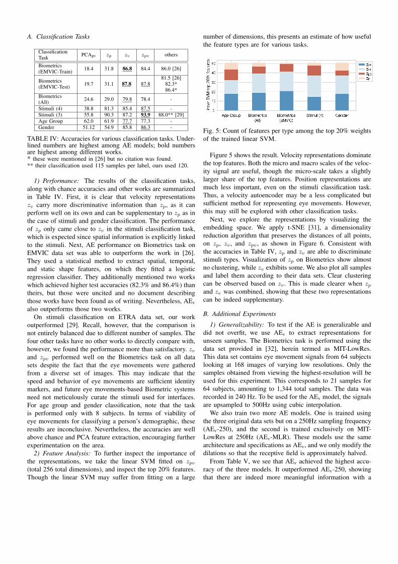
A. Classification Tasks

ClassificationTask PCApv zp zv zpv others

Biometrics(EMVIC-Train) 18.4 31.8 86.8 84.4 86.0 [26]

Biometrics(EMVIC-Test) 19.7 31.1 87.8 87.8

81.5 [26]82.3*86.4*

Biometrics(All) 24.6 29.0 79.8 78.4 -

Stimuli (4) 38.8 81.3 85.4 87.5 -Stimuli (3) 55.8 90.3 87.2 93.9 88.0** [29]Age Group 62.0 61.9 77.7 77.3 -Gender 51.12 54.9 85.8 86.3 -

TABLE IV: Accuracies for various classification tasks. Under-lined numbers are highest among AE models; bold numbersare highest among different works.* these were mentioned in [26] but no citation was found.** their classification used 115 samples per label, ours used 120.

1) Performance: The results of the classification tasks,along with chance accuracies and other works are summarizedin Table IV. First, it is clear that velocity representationszv carry more discriminative information than zp, as it canperform well on its own and can be supplementary to zp as inthe case of stimuli and gender classification. The performanceof zp only came close to zv in the stimuli classification task,which is expected since spatial information is explicitly linkedto the stimuli. Next, AE performance on Biometrics task onEMVIC data set was able to outperform the work in [26].They used a statistical method to extract spatial, temporal,and static shape features, on which they fitted a logisticregression classifier. They additionally mentioned two workswhich achieved higher test accuracies (82.3% and 86.4%) thantheirs, but those were uncited and no document describingthose works have been found as of writing. Nevertheless, AEvalso outperforms those two works.

On stimuli classification on ETRA data set, our workoutperformed [29]. Recall, however, that the comparison isnot entirely balanced due to different number of samples. Thefour other tasks have no other works to directly compare with,however, we found the performance more than satisfactory. zvand zpv performed well on the Biometrics task on all datasets despite the fact that the eye movements were gatheredfrom a diverse set of images. This may indicate that thespeed and behavior of eye movements are sufficient identitymarkers, and future eye movements-based Biometric systemsneed not meticulously curate the stimuli used for interfaces.For age group and gender classification, note that the taskis performed only with 8 subjects. In terms of viability ofeye movements for classifying a person’s demographic, theseresults are inconclusive. Nevertheless, the accuracies are wellabove chance and PCA feature extraction, encouraging furtherexperimentation on the area.

2) Feature Analysis: To further inspect the importance ofthe representations, we take the linear SVM fitted on zpv(total 256 total dimensions), and inspect the top 20% features.Though the linear SVM may suffer from fitting on a large

number of dimensions, this presents an estimate of how usefulthe feature types are for various tasks.

Fig. 5: Count of features per type among the top 20% weightsof the trained linear SVM.

Figure 5 shows the result. Velocity representations dominatethe top features. Both the micro and macro scales of the veloc-ity signal are useful, though the micro-scale takes a slightlylarger share of the top features. Position representations aremuch less important, even on the stimuli classification task.Thus, a velocity autoencoder may be a less complicated butsufficient method for representing eye movements. However,this may still be explored with other classification tasks.

Next, we explore the representations by visualizing theembedding space. We apply t-SNE [31], a dimensionalityreduction algorithm that preserves the distances of all points,on zp, zv , and zpv , as shown in Figure 6. Consistent withthe accuracies in Table IV, zp and zv are able to discriminatestimuli types. Visualization of zp on Biometrics show almostno clustering, while zv exhibits some. We also plot all samplesand label them according to their data sets. Clear clusteringcan be observed based on zv . This is made clearer when zpand zv was combined, showing that these two representationscan be indeed supplementary.

B. Additional Experiments

1) Generalizability: To test if the AE is generalizable anddid not overfit, we use AEv to extract representations forunseen samples. The Biometrics task is performed using thedata set provided in [32], herein termed as MIT-LowRes.This data set contains eye movement signals from 64 subjectslooking at 168 images of varying low resolutions. Only thesamples obtained from viewing the highest-resolution will beused for this experiment. This corresponds to 21 samples for64 subjects, amounting to 1,344 total samples. The data wasrecorded in 240 Hz. To be used for the AEv model, the signalsare upsampled to 500Hz using cubic interpolation.

We also train two more AE models. One is trained usingthe three original data sets but on a 250Hz sampling frequency(AEv-250), and the second is trained exclusively on MIT-LowRes at 250Hz (AEv-MLR). These models use the samearchitecture and specifications as AEv, and we only modify thedilations so that the receptive field is approximately halved.

From Table V, we see that AEv achieved the highest accu-racy of the three models. It outperformed AEv-250, showingthat there are indeed more meaningful information with a

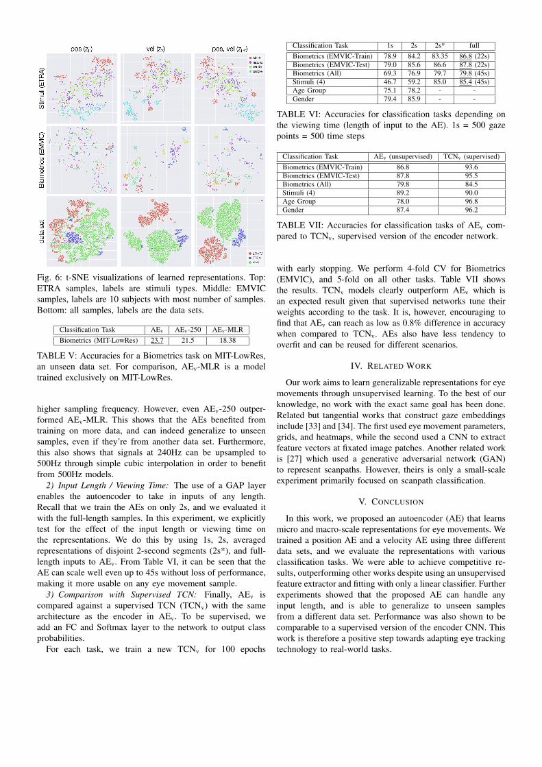
Fig. 6: t-SNE visualizations of learned representations. Top:ETRA samples, labels are stimuli types. Middle: EMVICsamples, labels are 10 subjects with most number of samples.Bottom: all samples, labels are the data sets.

Classification Task AEv AEv-250 AEv-MLRBiometrics (MIT-LowRes) 23.7 21.5 18.38

TABLE V: Accuracies for a Biometrics task on MIT-LowRes,an unseen data set. For comparison, AEv-MLR is a modeltrained exclusively on MIT-LowRes.

higher sampling frequency. However, even AEv-250 outper-formed AEv-MLR. This shows that the AEs benefited fromtraining on more data, and can indeed generalize to unseensamples, even if they’re from another data set. Furthermore,this also shows that signals at 240Hz can be upsampled to500Hz through simple cubic interpolation in order to benefitfrom 500Hz models.

2) Input Length / Viewing Time: The use of a GAP layerenables the autoencoder to take in inputs of any length.Recall that we train the AEs on only 2s, and we evaluated itwith the full-length samples. In this experiment, we explicitlytest for the effect of the input length or viewing time onthe representations. We do this by using 1s, 2s, averagedrepresentations of disjoint 2-second segments (2s*), and full-length inputs to AEv. From Table VI, it can be seen that theAE can scale well even up to 45s without loss of performance,making it more usable on any eye movement sample.

3) Comparison with Supervised TCN: Finally, AEv iscompared against a supervised TCN (TCNv) with the samearchitecture as the encoder in AEv. To be supervised, weadd an FC and Softmax layer to the network to output classprobabilities.

For each task, we train a new TCNv for 100 epochs

Classification Task 1s 2s 2s* fullBiometrics (EMVIC-Train) 78.9 84.2 83.35 86.8 (22s)Biometrics (EMVIC-Test) 79.0 85.6 86.6 87.8 (22s)Biometrics (All) 69.3 76.9 79.7 79.8 (45s)Stimuli (4) 46.7 59.2 85.0 85.4 (45s)Age Group 75.1 78.2 - -Gender 79.4 85.9 - -

TABLE VI: Accuracies for classification tasks depending onthe viewing time (length of input to the AE). 1s = 500 gazepoints = 500 time steps

Classification Task AEv (unsupervised) TCNv (supervised)Biometrics (EMVIC-Train) 86.8 93.6Biometrics (EMVIC-Test) 87.8 95.5Biometrics (All) 79.8 84.5Stimuli (4) 89.2 90.0Age Group 78.0 96.8Gender 87.4 96.2

TABLE VII: Accuracies for classification tasks of AEv com-pared to TCNv, supervised version of the encoder network.

with early stopping. We perform 4-fold CV for Biometrics(EMVIC), and 5-fold on all other tasks. Table VII showsthe results. TCNv models clearly outperform AEv which isan expected result given that supervised networks tune theirweights according to the task. It is, however, encouraging tofind that AEv can reach as low as 0.8% difference in accuracywhen compared to TCNv. AEs also have less tendency tooverfit and can be reused for different scenarios.

IV. RELATED WORK

Our work aims to learn generalizable representations for eyemovements through unsupervised learning. To the best of ourknowledge, no work with the exact same goal has been done.Related but tangential works that construct gaze embeddingsinclude [33] and [34]. The first used eye movement parameters,grids, and heatmaps, while the second used a CNN to extractfeature vectors at fixated image patches. Another related workis [27] which used a generative adversarial network (GAN)to represent scanpaths. However, theirs is only a small-scaleexperiment primarily focused on scanpath classification.

V. CONCLUSION

In this work, we proposed an autoencoder (AE) that learnsmicro and macro-scale representations for eye movements. Wetrained a position AE and a velocity AE using three differentdata sets, and we evaluate the representations with variousclassification tasks. We were able to achieve competitive re-sults, outperforming other works despite using an unsupervisedfeature extractor and fitting with only a linear classifier. Furtherexperiments showed that the proposed AE can handle anyinput length, and is able to generalize to unseen samplesfrom a different data set. Performance was also shown to becomparable to a supervised version of the encoder CNN. Thiswork is therefore a positive step towards adapting eye trackingtechnology to real-world tasks.

REFERENCES

[1] P. Konig, N. Wilming, T. Kietzmann, J. Ossandon, S. Onat, B. Ehinger,R. Gameiro, and K. Kaspar, “Eye movements as a window to cognitiveprocesses,” Journal of Eye Movement Research, vol. 9, no. 5, Dec.2016. [Online]. Available: https://bop.unibe.ch/JEMR/article/view/3383

[2] S. Hutton, “Cognitive control of saccadic eye movements,” Brain andCognition, vol. 68, no. 3, pp. 327–340, Dec. 2008. [Online]. Available:https://doi.org/10.1016/j.bandc.2008.08.021

[3] J. Otero-Millan, X. G. Troncoso, S. L. Macknik, I. Serrano-Pedraza,and S. Martinez-Conde, “Saccades and microsaccades during visualfixation, exploration, and search: Foundations for a common saccadicgenerator,” Journal of Vision, vol. 8, no. 14, pp. 21–21, Dec. 2008.[Online]. Available: https://doi.org/10.1167/8.14.21

[4] E. Siegenthaler, F. M. Costela, M. B. McCamy, L. L. D. Stasi, J. Otero-Millan, A. Sonderegger, R. Groner, S. Macknik, and S. Martinez-Conde,“Task difficulty in mental arithmetic affects microsaccadic rates andmagnitudes,” European Journal of Neuroscience, vol. 39, no. 2, pp. 287–294, Nov. 2013. [Online]. Available: https://doi.org/10.1111/ejn.12395

[5] S. Martinez-Conde and S. L. Macknik, “Unchanging visions: the effectsand limitations of ocular stillness,” Philosophical Transactions of theRoyal Society B: Biological Sciences, vol. 372, no. 1718, p. 20160204,Feb. 2017. [Online]. Available: https://doi.org/10.1098/rstb.2016.0204

[6] K. Krejtz, A. T. Duchowski, A. Niedzielska, C. Biele, and I. Krejtz,“Eye tracking cognitive load using pupil diameter and microsaccadeswith fixed gaze,” PLOS ONE, vol. 13, no. 9, p. e0203629, Sep. 2018.[Online]. Available: https://doi.org/10.1371/journal.pone.0203629

[7] A. T. Duchowski, Eye Tracking Methodology. Springer InternationalPublishing, 2017. [Online]. Available: https://doi.org/10.1007/978-3-319-57883-5

[8] Rigas, Ioannis; Texas State University, Friedman, Lee; TexasState University, and Komogortsev, Oleg; Texas State University,“Study of an extensive set of eye movement features: Extractionmethods and statistical analysis,” 2018. [Online]. Available: https://bop.unibe.ch/JEMR/article/view/3795

[9] O. L. Meur and T. Baccino, “Methods for comparing scanpathsand saliency maps: strengths and weaknesses,” Behavior ResearchMethods, vol. 45, no. 1, pp. 251–266, Jul. 2012. [Online]. Available:https://doi.org/10.3758/s13428-012-0226-9

[10] N. C. Anderson, F. Anderson, A. Kingstone, and W. F. Bischof,“A comparison of scanpath comparison methods,” Behavior ResearchMethods, vol. 47, no. 4, pp. 1377–1392, Dec. 2014. [Online]. Available:https://doi.org/10.3758/s13428-014-0550-3

[11] V. Cantoni, C. Galdi, M. Nappi, M. Porta, and D. Riccio, “GANT:Gaze analysis technique for human identification,” Pattern Recognition,vol. 48, no. 4, pp. 1027–1038, Apr. 2015. [Online]. Available:https://doi.org/10.1016/j.patcog.2014.02.017

[12] A. Coutrot, J. H. Hsiao, and A. B. Chan, “Scanpath modelingand classification with hidden markov models,” Behavior ResearchMethods, vol. 50, no. 1, pp. 362–379, Apr. 2017. [Online]. Available:https://doi.org/10.3758/s13428-017-0876-8

[13] R. Andersson, L. Larsson, K. Holmqvist, M. Stridh, and M. Nystrom,“One algorithm to rule them all? an evaluation and discussion often eye movement event-detection algorithms,” Behavior ResearchMethods, vol. 49, no. 2, pp. 616–637, May 2016. [Online]. Available:https://doi.org/10.3758/s13428-016-0738-9

[14] R. S. Hessels, D. C. Niehorster, M. Nystrom, R. Andersson, andI. T. C. Hooge, “Is the eye-movement field confused about fixationsand saccades? a survey among 124 researchers,” Royal Society OpenScience, vol. 5, no. 8, p. 180502, Aug. 2018. [Online]. Available:https://doi.org/10.1098/rsos.180502

[15] Y. Bengio, A. Courville, and P. Vincent, “Representation learning: Areview and new perspectives,” IEEE Transactions on Pattern Analysisand Machine Intelligence, vol. 35, no. 8, pp. 1798–1828, Aug. 2013.[Online]. Available: https://doi.org/10.1109/tpami.2013.50

[16] S. Bai, J. Z. Kolter, and V. Koltun, “An empirical evaluation of genericconvolutional and recurrent networks for sequence modeling,” 2018.

[17] V. Dumoulin and F. Visin, “A guide to convolution arithmetic for deeplearning,” 2016.

[18] P. Kasprowski and K. Harezlak, “The second eye movementsverification and identification competition,” in IEEE International JointConference on Biometrics. IEEE, Sep. 2014. [Online]. Available:https://doi.org/10.1109/btas.2014.6996285

[19] M. Cerf, J. Harel, W. Einhauser, and C. Koch, “Predicting human gazeusing low-level saliency combined with face detection,” in Advances inneural information processing systems, 2008, pp. 241–248.

[20] M. B. McCamy, J. Otero-Millan, L. L. D. Stasi, S. L. Macknik,and S. Martinez-Conde, “Highly informative natural scene regionsincrease microsaccade production during visual scanning,” Journal ofNeuroscience, vol. 34, no. 8, pp. 2956–2966, Feb. 2014. [Online].Available: https://doi.org/10.1523/jneurosci.4448-13.2014

[21] S. Ioffe and C. Szegedy, “Batch normalization: Accelerating deepnetwork training by reducing internal covariate shift,” 2015.

[22] K. He, X. Zhang, S. Ren, and J. Sun, “Deep residual learningfor image recognition,” 2016 IEEE Conference on Computer Visionand Pattern Recognition (CVPR), Jun 2016. [Online]. Available:http://dx.doi.org/10.1109/cvpr.2016.90

[23] L. A. Jager, S. Makowski, P. Prasse, S. Liehr, M. Seidler, and T. Scheffer,“Deep eyedentification: Biometric identification using micro-movementsof the eye,” Lecture Notes in Computer Science, p. 299–314, 2020.

[24] D. P. Kingma and J. Ba, “Adam: A method for stochastic optimization,”2014.

[25] A. Paszke, S. Gross, F. Massa, A. Lerer, J. Bradbury, G. Chanan,T. Killeen, Z. Lin, N. Gimelshein, L. Antiga et al., “Pytorch: Animperative style, high-performance deep learning library,” in Advancesin neural information processing systems, 2019, pp. 8026–8037.

[26] S. Mukhopadhyay and S. Nandi, “LPiTrack: Eye movement patternrecognition algorithm and application to biometric identification,”Machine Learning, vol. 107, no. 2, pp. 313–331, Jun. 2017. [Online].Available: https://doi.org/10.1007/s10994-017-5649-1

[27] W. Fuhl, E. Bozkir, B. Hosp, N. Castner, D. Geisler, T. C. Santini, andE. Kasneci, “Encodji,” in Proceedings of the 11th ACM Symposium onEye Tracking Research & Applications. ACM, Jun. 2019. [Online].Available: https://doi.org/10.1145/3314111.3323074

[28] A. Kumar, A. Tyagi, M. Burch, D. Weiskopf, and K. Mueller,“Task classification model for visual fixation, exploration, and search,”in Proceedings of the 11th ACM Symposium on Eye TrackingResearch & Applications. ACM, Jun. 2019. [Online]. Available:https://doi.org/10.1145/3314111.3323073

[29] D. Geisler, N. Castner, G. Kasneci, and E. Kasneci, “A MinHashapproach for fast scanpath classification,” in Symposium on EyeTracking Research and Applications. ACM, Jun. 2020. [Online].Available: https://doi.org/10.1145/3379155.3391325

[30] F. Pedregosa, G. Varoquaux, A. Gramfort, V. Michel, B. Thirion,O. Grisel, M. Blondel, P. Prettenhofer, R. Weiss, V. Dubourg, J. Vander-plas, A. Passos, D. Cournapeau, M. Brucher, M. Perrot, and E. Duch-esnay, “Scikit-learn: Machine learning in Python,” Journal of MachineLearning Research, vol. 12, pp. 2825–2830, 2011.

[31] L. v. d. Maaten and G. Hinton, “Visualizing data using t-sne,” Journalof machine learning research, vol. 9, no. Nov, pp. 2579–2605, 2008.

[32] T. Judd, F. Durand, and A. Torralba, “Fixations on low resolutionimages,” Journal of Vision, vol. 10, no. 7, pp. 142–142, Aug. 2010.[Online]. Available: https://doi.org/10.1167/10.7.142

[33] N. Karessli, Z. Akata, B. Schiele, and A. Bulling, “Gaze embeddingsfor zero-shot image classification,” 2017 IEEE Conference on ComputerVision and Pattern Recognition (CVPR), Jul 2017. [Online]. Available:http://dx.doi.org/10.1109/CVPR.2017.679

[34] N. Castner, T. C. Kuebler, K. Scheiter, J. Richter, T. Eder, F. Huettig,C. Keutel, and E. Kasneci, “Deep semantic gaze embedding andscanpath comparison for expertise classification during opt viewing,”Symposium on Eye Tracking Research and Applications, Jun 2020.[Online]. Available: http://dx.doi.org/10.1145/3379155.3391320