Int J Comput VisDOI 10.1007/s11263-009-0268-3

Gaussian Processes for Object Categorization

Ashish Kapoor · Kristen Grauman · Raquel Urtasun ·Trevor Darrell

Received: 22 July 2008 / Accepted: 1 July 2009© The Author(s) 2009. This article is published with open access at Springerlink.com

Abstract Discriminative methods for visual object categoryrecognition are typically non-probabilistic, predicting classlabels but not directly providing an estimate of uncertainty.Gaussian Processes (GPs) provide a framework for derivingregression techniques with explicit uncertainty models; weshow here how Gaussian Processes with covariance func-tions defined based on a Pyramid Match Kernel (PMK) canbe used for probabilistic object category recognition. Ourprobabilistic formulation provides a principled way to learnhyperparameters, which we utilize to learn an optimal com-bination of multiple covariance functions. It also offers con-fidence estimates at test points, and naturally allows for anactive learning paradigm in which points are optimally se-lected for interactive labeling. We show that with an appro-priate combination of kernels a significant boost in classi-fication performance is possible. Further, our experimentsindicate the utility of active learning with probabilistic pre-dictive models, especially when the amount of training datalabels that may be sought for a category is ultimately verysmall.

A. Kapoor (�)Microsoft Research, Redmond, WA 98052, USAe-mail: akapoor@microsoft.com

K. GraumanUniversity of Texas at Austin, Austin, TX 78712, USAe-mail: grauman@cs.utexas.edu

R. Urtasun · T. DarrellUC Berkeley EECS & ICSI, Berkeley, CA 94720, USA

R. Urtasune-mail: rurtasun@csail.mit.edu

T. Darrelle-mail: trevor@eecs.berkeley.edu

Keywords Object recognition · Gaussian process · Kernelcombination · Active learning

1 Introduction

Object categorization is a fundamental problem in imageunderstanding. It remains a challenging learning task givenboth the variability of images that objects from the sameclass can produce, as well as the substantial expense ofproviding high quality image annotations needed to trainaccurate models. Discriminative methods for visual cat-egory learning have yielded promising results in recentyears, including various approaches based on support vec-tor machines or nearest neighbor classification (Graumanand Darrell 2005; Zhang et al. 2006; Wallraven et al. 2003;Nister and Stewenius 2006; Lazebnik et al. 2006; Varmaand Ray 2007; Bosch et al. 2007; Frome et al. 2007; Ku-mar and Sminchisescu 2007). However, such methods typi-cally are not explicitly probabilistic, which makes them in-adequate when estimates of uncertainty are required. At thesame time, probabilistic generative methods that attempt todirectly model the joint distribution of object classes andtheir features—though appealing for their ability to estimateuncertainty during inference—can be impractical for imagerecognition applications due to the complexity of represent-ing the data’s underlying density.

In this work we provide a probabilistic discriminative ap-proach to object categorization, with the goal of exercisingthe advantages of both types of methods. We introduce anew Gaussian Process (GP) regression method for objectcategory recognition using a local feature correspondencekernel. Local feature-based object recognition has severalimportant advantages, including invariance to various trans-lational, rotational, affine and photometric transformations,

Int J Comput Vis

and robustness to partial occlusions. Our method is basedon a GP with a covariance function derived from a Pyra-mid Match Kernel (Grauman and Darrell 2005), which of-fers an efficient approximation to a partial-match distancefunction and can therefore handle outliers and occlusions.Our model offers some of the known benefits of probabilis-tic techniques, while still maintaining the power of a dis-criminative learner. In particular, we show how it enablesboth active visual category learning, as well as learning frommultiple image feature sources with an optimal combinationof covariance functions.

Collecting training data for large-scale image categorymodels is a potentially expensive process. While certain cat-egories may have a large number of training images avail-able, many more will have relatively few. A number of inge-nious schemes have been developed to obtain labeled datafrom people performing other tasks (e.g., von Ahn et al.2006; von Ahn and Dabbish 2004), or directly labeling ob-jects in images (http://labelme.csail.mit.edu/). To make themost of scarce human labeling resources it is imperative tocarefully select points for user labeling. The paradigm ofactive learning has been introduced in the machine learn-ing community to address this issue (Freund et al. 1997;Tong and Koller 2000; McCallum and Nigam 1998; Musleaet al. 2002; Zhu et al. 2003); with an active learning method,generally new test points are selected so as to minimize themodel entropy.

GPs have received limited attention in the computer vi-sion literature to date perhaps due to the fact that they areconventionally limited to modest amounts of training data:the learning complexity is O(n3), cubic in the number oftraining examples. While recent advances in sparse GPs arepromising (e.g., Lawrence et al. 2002; Shen et al. 2006;Snelson and Ghahramani 2006; Urtasun and Darrell 2008),we focus here on the case of active learning with relativelysmall numbers of labeled examples (10–100), which is fea-sible with existing implementations. In this realm, we showthat active learning provides significantly more accurate es-timates per labeled point than does a conventional randomselection of training points.

Specific choices made regarding image representationsand kernel parameters can greatly influence a classifier’s po-tential. Even within the domain of local image features andmatching kernels, a variety of alternative interest point de-tectors, descriptors, match criteria, and feature space quanti-zation strategies are available. Rather than require a user todecide a priori which particular items will define the GP’scovariance function, we show how to automatically optimizethe combination of kernels for the recognition task using theGP marginal likelihood function. As a result, one can com-pute a set of potential kernels using a variety of local fea-ture types, and then directly learn a weight for each suchthat the final combination is highly discriminative. While

recent work has considered multiple kernel learning (Varmaand Ray 2007; Kumar and Sminchisescu 2007) and cross-validation approaches (Bosch et al. 2007) to combine imagefeature types within SVM classifiers, to our knowledge ourapproach is the first to consider kernel combinations in aprobabilistic setting.

The three main contributions of this paper are (1) a prob-abilistic discriminative category recognition scheme basedon a Gaussian Process prior with a covariance function de-fined using the Pyramid Match Kernel, (2) the introductionof an active learning paradigm for object category learningwhich optimally selects unlabeled test points for interactivelabeling, and (3) a probabilistic approach to learn discrim-inative kernel combinations for multiple local feature typeswithin a GP framework. We show that with active learningsmall amounts of interactively labeled data can provide veryaccurate category recognition performance, while with co-variance functions that optimally combine multiple match-ing kernels our method obtains state-of-the-art results withbenchmark datasets.

2 Previous Work

Object category recognition has been a topic of active in-terest in the computer vision literature. Methods based onlocal feature descriptors (cf. Lowe 2004; Mikolajczyk andSchmid 2001) have been shown to offer invariance across arange of geometric and photometric conditions. Early mod-els captured appearance and shape variation in a generativeprobabilistic framework (Fergus et al. 2003), but more re-cent techniques have typically exploited methods based onSVMs or nearest neighbors in a bag-of-visual-words fea-ture space (Sivic and Zisserman 2003; Nister and Stewenius2006; Zhang et al. 2006; Moosmann and Jurie 2007).

Several authors have explored correspondence-based ker-nels (Zhang et al. 2006; Wallraven et al. 2003), wherethe distance between a set of local feature descriptors—potentially including appearance and shape/position—iscomputed based on associating pairs of descriptors. How-ever, the polynomial-time computational cost of correspond-ence-based distance measures makes them unsuitable fordomains where there are large databases or large numbersof features per image. In Grauman and Darrell (2005) theauthors introduced the Pyramid Match Kernel (PMK), anefficient linear-time approximation to a partial match cor-respondence, and in Lazebnik et al. (2006) it was demon-strated that a spatial variant—which efficiently representsthe distinction between appearance and image locationfeatures—outperformed many competing m-ethods.

Semi-supervised or unsupervised visual category learn-ing methods are related to active learning, in that they alsoleverage unlabeled examples to learn more accurately when

Int J Comput Vis

limited labeled examples are available. Generative modelswhich model visual words as arising from a set of underlyingobjects or “topics” based on recently introduced methods forLatent Dirichlet Allocation have been developed (Sivic et al.2005; Sudderth et al. 2005) but as yet have not been appliedto active learning nor evaluated on purely supervised tasks.A semi-supervised method using normalized cuts to clustera graph defined by Pyramid Match distances between exam-ples was presented in Grauman and Darrell (2006b), but thismethod is not probabilistic nor does it provide for an activelearning formalism.

In the machine learning literature active learning has beena topic of recent interest, and numerous schemes have beenproposed for choosing unlabeled points for tagging. For ex-ample, in Freund et al. (1997) the authors propose using thedisagreement among the committee of classifiers as a cri-terion for active learning, and show an application to im-age classification (Abramson and Freund 2004). In Tongand Koller (2000), unlabeled examples to query are selectedbased on minimizing the version space within the SVM for-mulation, while in Chang et al. (2005) an SVM-based activelearner is applied for image retrieval using color and texturefeatures.

Within the Gaussian Process framework, the method ofchoice has been to look at the expected informativeness of anunlabeled data point (Lawrence et al. 2002; MacKay 1992).Specifically, the idea is to choose to query cases that areexpected to maximally influence the posterior distributionover the set of possible classifiers. Additional studies havesought to combine active learning with semi-supervisedlearning (McCallum and Nigam 1998; Muslea et al. 2002;Zhu et al. 2003). Our work is significantly different as wefocus on local feature approaches for the task of object cat-egorization. We explore the GP models, which provide es-timates for uncertainty in prediction and can be easily ex-tended to active learning.

Recent work has shown the value of combining multi-ple local image feature types into a single kernel matrix,either by using cross-validation with a held-out set of la-beled images to adjust the weight attached to each (Boschet al. 2007), or by optimizing the weights to align the com-bined kernel with the ideal kernel matrix reflecting the la-bels on the training data (Kumar and Sminchisescu 2007;Lin et al. 2007; Varma and Ray 2007). Both tactics haveyielded impressive results in practice. Our proposed methodto optimize kernel weights fits directly within our GP learn-ing framework, and is distinct in that rather than target thelabels of training examples, it maximizes the evidence of theprobabilistic model.

Gaussian Processes have been recently introduced to thecomputer vision literature. While they have been used in Ur-tasun et al. (2005, 2006) for human motion modeling, gen-der classification (Kim et al. 2006) and in Williams (2006)

for stereo segmentation, we are unaware of any prior workon visual object recognition in a Gaussian Process frame-work.1

3 Approach Overview

Gaussian Processes provide an appealing probabilisticframework where the uncertainty is modeled conditionedon the observations. This circumvents the need to ex-plicitly model the probability distribution of observations,which are often high-dimensional. Some popular GP mod-els include GP classification and regression (Rasmusen andWilliams 2006), non-linear dimensionality reduction us-ing the Gaussian Process Latent Variable Model (GPLVM)(Lawrence 2004), and Mixture of GPs (Tresp 2000). In thecontext of this work, the Gaussian Process classificationand regression framework is especially appealing as it canbe considered a probabilistic counterpart to Support Vec-tor Machines (SVM) and its variants, which have alreadybeen thoroughly used with much success for object recog-nition tasks. Beyond providing good accuracy, GP modelsfor classification and regression are probabilistic, and alsoenjoy the benefits common to all kernel-based models.

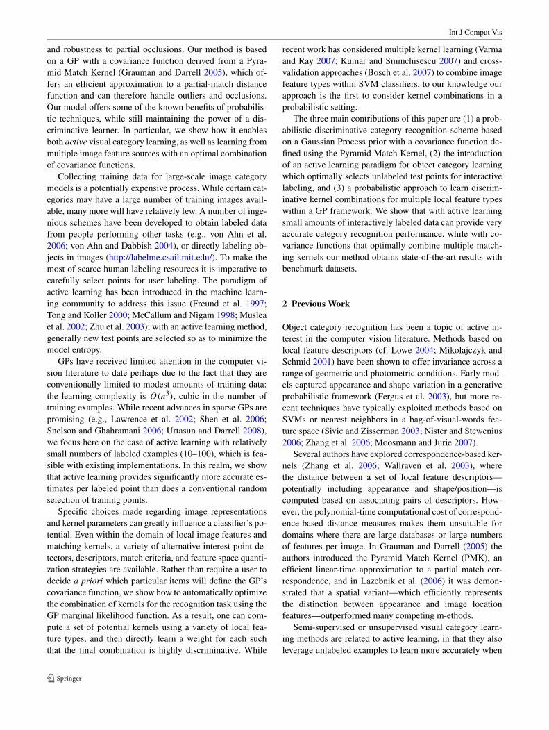
The main idea of our approach is to construct proba-bilistic discriminative classifiers for object recognition us-ing Gaussian Process priors, with covariance functions de-fined by the Pyramid Match Kernel (GP-PMK). In additionto offering a novel approach to supervised visual categorylearning, we show how this framework also allows both thelearning of optimal combinations of covariance functions,as well as an active learning strategy—which is especiallypreferable when minimal labeling effort is available. Fig-ure 1 shows the proposed framework for active image cate-gorization. Given a pool of images of which few are labeled,the system aims to actively seek labels for unlabeled imagesby considering information from both the labeled and unla-beled sets of images. With the uncertainty estimates the GPclassifier provides, we are able to designate an active learn-ing criterion to focus labeling efforts on the most ambiguousunlabeled examples.

In the next section we review classification using GP pri-ors and discuss the distributions and parameters we employfor our model. Then in Sect. 5 we present our GP-PMKmodel, which is directly suitable for supervised learningwith or without active learning. Then in Sect. 6 we describehow to optimize the weights to combine multiple matchingkernels computed from different feature sets. Finally, we

1This paper expands on our previous conference publication (Kapoor etal. 2007); here we provide further explanation of our Gaussian Processmodel, extend it to allow combinations of multiple kernel functions,and report and discuss a number of additional experiments.

Int J Comput Vis

Fig. 1 The active learning framework. The goal of the system is toquery labels for images that are most useful in training

derive an active learning variant that can optimally selectpoints for interactive labeling in Sect. 7.

Note that throughout we assume that there is one primaryobject of interest in an image. Handling multiple objects inthe same image is also an interesting and challenging prob-lem, and will be the focus of future work.

4 Categorization with Gaussian Processes

Gaussian Process (GP) classification is related to kernel ma-chines such as Support Vector Machines (SVMs) (Evgeniouet al. 2000) and Regularized Least Square Classification(RLSC) and has been well-explored in machine learning. Incontrast to these methods, GPs provide probabilistic predic-tion estimates and thus are well-suited for active learning.In this section we briefly review regression and classifica-tion with Gaussian Process priors and describe our modelchoices.

Given a set of labeled data points XL = {x1, . . . ,xn},with class labels tL = {t1, . . . , tn}, we are interested in clas-sifying the unlabeled data xu. Under the Bayesian para-digm, we are interested in the distribution p(tu|X, tL). HereX = {XL,xu}, and tu is the random variable denoting theclass label for the unlabeled point xu. For sake of simplicityin discussion we limit ourselves to two-way classification,hence, the labels are ti ∈ {−1,1}, but this can be extendedto multi-label classification; see Rasmusen and Williams(2006) for a detailed discussion.

With GP models, a discrete label t for a data point xcan be considered to be generated via a continuous hid-den random variable y. The soft-hidden label arises due to aGaussian Process, which in turn imposes a smoothness con-straint on the possible solutions. A likelihood model p(t |y)

characterizes the relationship between the soft label y and

the observed annotation t . Thus, when we infer the label tufor the unlabeled data point xu, we probabilistically combinethe smoothness constraint and the information obtained byobserving the annotations tL.

4.1 Smoothness Constraints via the GP Prior

There exist two different perspectives for regression andclassification with Gaussian Process: the process perspec-tive and the weight perspective. We overview both in thefollowing in order to provide background on the basic con-cepts underlying the GP model.

The process perspective: The smoothness constraint is im-posed using a Gaussian Process prior that defines the proba-bilistic relationship between the images X and the soft labelsY. The distribution p(Y|X) gives higher probability to thelabelings that respect the similarity between the data points.Intuitively, the assumption is that similar data points shouldhave the same class assignments/regression values; the sim-ilarity between two points xi and xj is defined via a kernelk(xi ,xj ). Probabilistic constraints are imposed on the col-lection of soft labels Y = {y1, . . . , yn, yu}. In particular, thesoft labels are assumed to be jointly Gaussian and the co-variance between two outputs yi and yj is typically speci-fied using a kernel function2 applied to xi and xj . Formally,p(Y|X) ∼ N (0,K) where K is a (n + 1)-by-(n + 1) kernelmatrix with Kij = k(xi ,xj ), and n + 1 reflects the n labeledexamples and one unlabeled example.

The weight perspective: What we have described above isthe process perspective for regression and classification withthe GP priors. An alternate but mathematically equivalentinterpretation is based on the weight perspective. In this per-spective the hidden soft-label y arises due to application of afunction f (·) directly on the input data point (i.e. y = f (x)),which takes the form of a linear combination of orthonormalbasis functions:

f (x) =∑

k

wkν1/2k φk(x) = wT �(x), (1)

where φk are the eigenfunctions of the operator inducedby k in the Reproducing Kernel Hilbert Space (Evgeniouet al. 2000), νk are the corresponding eigenvalues, wk arethe weights, and �(x) = [ν1/2

1 φ1(x), ν1/22 φ2(x), . . .]T . Note

that the dimensionality of the basis can be infinite. As-suming a spherical Gaussian prior over the weights, that isw = [w1,w2, . . .]T ∼ N (0, I), it can be shown that the hid-den soft labels Y (which result from evaluation of the func-tion f (·) on the input data points X) are jointly Gaussian

2One can use a non-parametric covariance function, but the number ofparameters to estimate grows exponentially with the amount of trainingdata.

Int J Comput Vis

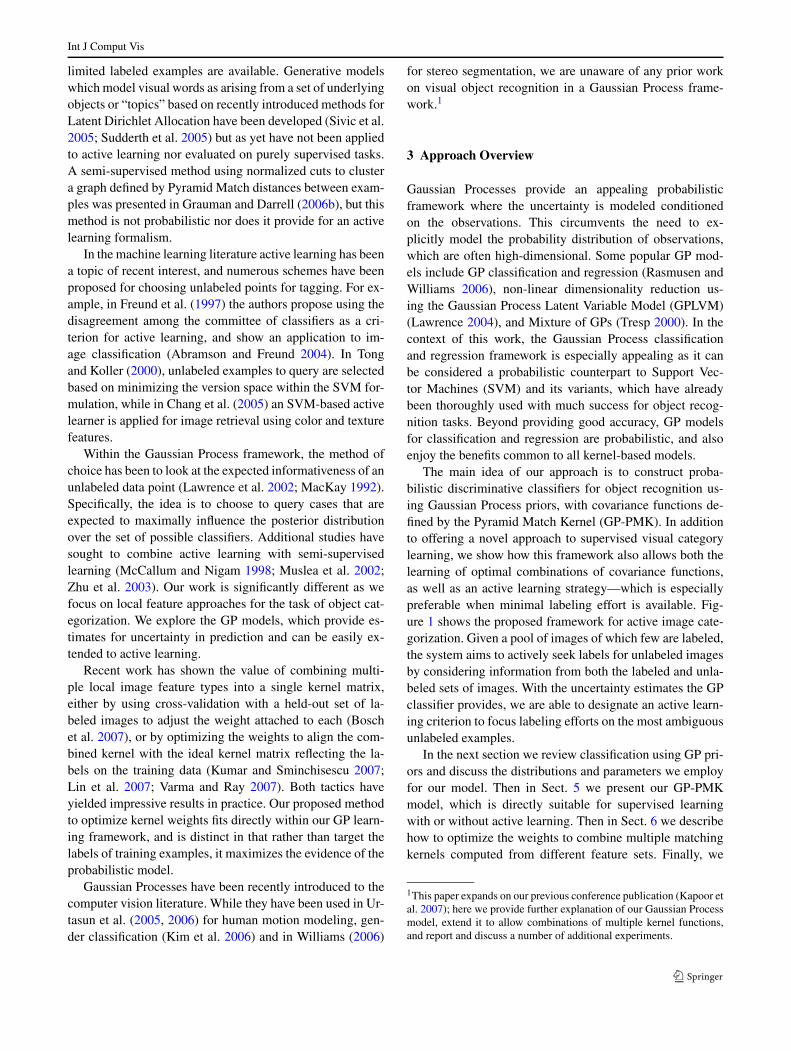
Fig. 2 Graphical models in plate notation for classification viaGaussian Processes. The rounds and squares represent continu-ous and discrete random variables, respectively. A filled (unfilled)round/square denotes that the random variable is fully observed (un-observed). X = {x1, . . . ,xn,xu} is the set of all images and is ob-

served for both labeled and unlabeled data points. The correspond-ing Y = {y1, . . . , yn, yu} is completely unobserved and the labels{t1, . . . , tn} are observed only for the training images {xi , . . . ,xn}and unobserved for the unlabeled image xu

with zero mean and with the covariance given by the kernelmatrix K.

These two different but equivalent perspectives for re-gression and classification with the GP priors are illustratedin Fig. 2. Both views lead to different implementations, butare conceptually equivalent. The process perspective is eas-ier to implement for the cases when K is non-parametric orwhen it is difficult to determine �(x). Similarly, difficultyarises in using the weights perspective when �(x) is high di-mensional (possibly infinite dimensional). In such cases it iseasier to follow the process perspective as inference over thelabels can be done by computing the kernel matrix, whichcircumvents the need to explicitly evaluate the eigenfunc-tions. In our work we determine similarities between imagesusing primarily non-parametric techniques for which the ex-plicit form of the eigenfunctions is unknown. Thus, in thiswork, we follow the process perspective. For details, pleasesee Seeger (2004).

4.2 The Likelihood Model

The likelihood models the probabilistic relationship be-tween the observed label t and the hidden label y. The ma-jority of the likelihood models proposed for GP classifica-tion use additional latent “squashing” variables that trans-form unconstrained variables into labels. A wide range ofsquashing functions have been developed in the literature(Rasmusen and Williams 2006) and examples include thelogistic and the probit functions. To make predictions basedon the training set for a test set in these models (i.e., pro-bit and logit) one has to integrate out the prediction over the

posterior. Since the likelihood is not Gaussian, neither theposterior, the marginal likelihood, nor the predictions canbe computed analytically. Instead, one has to rely on numer-ical methods, such as MCMC (Williams and Barber 1998),or approximations of the posterior, e.g. Laplace and Expec-tation Propagation (Minka 2001).

In contrast to GP classification, GP regression leadsto efficient analytic solutions for prediction. For GaussianProcess regression using a Gaussian noise model, the rela-tion between t and y is given by

p(t |y) = 1√2πσ 2

e− (t−y)2

2σ2 , (2)

where σ is the noise model variance. Since this likelihoodmodel is Gaussian, it leads to a closed form solution for in-ference. Although originally developed for regression, theGaussian noise model has also proven effective for classi-fication,3 and its performance typically matches the morecomplex probit and logit likelihood models noted above.Due to its simplicity and good performance, in our exper-iments we use regression (i.e., the Gaussian noise model) tolabel variables. Non-Gaussian noise models could also beapplied within the proposed framework, and exploring themis a topic of interest for future work.

3This method is referred to as least-squares classification in the lit-erature (see Sect. 6.5 of Rasmusen and Williams 2006) and oftendemonstrates performance competitive with more expensive GaussianProcess classification methods that require approximate inference.

Int J Comput Vis

4.3 Inference

Given the labeled and unlabeled data points, our goal is thento infer p(tu|X, tL). Specifically:

p(tu|X, tL) ∝∫

Yp(tu|Y)p(Y|X, tL). (3)

For a Gaussian noise model we can compute this integralusing closed form expressions. Note that the key quantity tocompute is the posterior p(Y|X, tL), which can be writtenas:

p(Y|X, tL) ∝ p(Y|X)p(tL|Y) = p(Y|X)

n∏

i=1

p(ti |yi). (4)

This equation probabilistically combines the smoothnessconstraints p(Y|X) imposed via the GP prior and the in-formation provided in the labels (p(tL|Y)). The posterior asshown in (4) is simply a product of Gaussians, and the pos-terior over the soft label yu has a particularly simple form.Specifically, p(yu|X, tL) ∼ N (yu, σ

2u ), where:

yu = k(xu)T (σ 2I + KLL)−1tL, (5)

�u = k(xu,xu) − k(xu)T (σ 2I + KLL)−1k(xu). (6)

Here, k(xu) is the vector of kernel function evaluations withn training points, and KLL = {k(xi ,xj )}, is the training co-variance, with xi ,xj ∈ Xu. Further, due to the Gaussiannoise model that links tu to yu, the predictive distributionover the unknown label tu is also a Gaussian: p(tu|X, tL) ∼N (yu,�u + σ 2).

Note that the posterior mean for both tu and yu is thesame; thus, the unlabeled point xu can be classified accord-ing to the sign of yu. Note that despite the fact that weonly consider sign of the posterior mean for classification,the uncertainties modeled using the GP prove very useful inperforming two key tasks. First, GPs inherently provide aprincipled way to do kernel combination as the probabilis-tic framework allows us to determine how well a particu-lar combination of kernels explains the data well. Secondly,unlike the Regularized Least Square Classification (RLSC)methods we also get the variance in prediction. As we willshow in Sect. 7, we can exploit these measures of uncer-tainty to guide an active learning procedure.

4.4 Training with the Gaussian Process Models

The performance of Gaussian Process-based classificationdepends upon the chosen kernel used to capture the similar-ity between examples, as well as the kernel’s hyperparame-ters, such as the length-scale, the noise variance, and otherparameters determining local feature-based image similar-ity. Finding the right set of all these parameters can be a

challenge. Many discriminative models (including SVMs)often use cross-validation, which is a robust measure butcan be prohibitively expensive and problematic when wehave few labeled data points. Learning in a Gaussian Processframework is equivalent to choosing the kernel hyperpara-meters of the covariance function. Ideally we would like tomarginalize over these hyperparameters. While approachesbased on Hybrid Monte Carlo have been explored to per-form this marginalization (Williams and Barber 1998), suchtechniques are relatively expensive.

Empirical Bayes is a more computationally efficient al-ternative where the idea is to maximize the marginal like-lihood or the evidence, which is nothing but the constantp(tL|X) that normalizes the posterior. This methodology oftuning the hyperparameter is often called evidence maxi-mization, and has been one of the favorite tools for perform-ing model selection. Evidence is a numerical quantity andsignifies how well a model fits the given data. By comparingthe evidence corresponding to the different models (or hy-perparameters that determine the model), we can choose themodel and the hyperparameters suitable for the task.

The idea is to choose a set of hyperparameters � thatmaximize the evidence: � = arg max� log[p(tL|X,�)].Note that the log evidence log(p(tL|X,�)) can be writtenas a closed form equation for the Gaussian noise model (GPregression):

logp(tL|X,�) = − 1

2tTL(σ 2I + KLL)−1tL

− 1

2log |σ 2I + KLL| − Const.

This objective can be maximized using non-linear optimiza-tion techniques, such as gradient descent. In this work, weuse gradient-descent to maximize evidence. The optimiza-tion procedure can perform multiple searches with differ-ent initializations to deal with the fact that the evidence willhave multiple local optima.

This scheme of learning hyperparameters by maximizingevidence lets us find the correct parameters without the needof cross-validation. Further, this procedure can also be usedto learn an ideal linear combination of covariance functions,which is a useful tool in practice to combine various localfeature object categorization schemes. We show this combi-nation strategy in Sect. 6.

5 Pyramid Match Kernel Gaussian Processes(GP-PMK)

To use GPs for object categorization, we need to define asuitable covariance function. We would like to exploit lo-cal feature methods for object and image representations.However, GP priors require covariance functions which are

Int J Comput Vis

positive semi-definite (a Mercer kernel) and traditional co-variance functions (e.g., RBF) are not suitable for represen-tations that are comprised of sets of features.

We wish to define a GP with a covariance function basedon a partial match distance function. The idea is to first rep-resent an image as an unordered set of local features, andthen use a matching over these sets of features to computea smoothness prior between images. The optimal least-costpartial matching takes two sets of features, possibly of vary-ing sizes, and pairs each point in the smaller set to a uniquepoint in the larger one, such that the sum of the distancesbetween the matched points is minimized. The cubic costof the optimal matching makes it prohibitive for recognitionwith a large number of local image features, yet rich imagedescriptions comprised of densely sampled local features areknown to often yield better recognition accuracy (Nowak etal. 2006).

Therefore, rather than adopt a full partial match kernel forthe GP prior, we use the Pyramid Match (Grauman and Dar-rell 2005). The Pyramid Match is a linear-time kernel func-tion over unordered feature sets that approximates the simi-larity measured by the optimal partial matching, and it formsa Mercer kernel. A multi-resolution partition (pyramid)carves the feature space into increasingly larger regions. Atthe finest resolution level in the pyramid, the partitions arevery small; at successive levels they continue to grow in sizeuntil a single partition encompasses the entire feature space.The insight of the Pyramid Match algorithm is to treat pointswhich share a bin in this pyramid as being matched, andto use the histograms to read off the number of possiblematches without explicitly searching for correspondences.Histogram intersection (the sum of the minimum number ofpoints in a given histogram bin) is used to count the numberof new matches that occur at each resolution level.

The input space S contains sets of feature vectors drawnfrom feature space F : S = {F|F = {f1, . . . , fm}}, where eachfeature fi ∈ F ⊆ �d , and m = |F|. For example, F mightbe the space of SIFT (Lowe 2004) descriptors (d = 128), orimage coordinate positions (d = 2), etc.; a set F contains acollection of these descriptors extracted from a single imageor object. An L-level histogram pyramid for input exampleF ∈ S is defined as: (F) = [H0(F), . . . ,HL−1(F)], whereHi(F) is a histogram vector formed over points in F usingmulti-dimensional bins.

The Pyramid Match Kernel (PMK) value between twoinput sets F1, F2 ∈ S is defined as the weighted sum of thenumber of feature matches found at each level of their pyra-mids (Grauman and Darrell 2005):

K ((F1),(F2))

=L−1∑

i=0

wi

(I (Hi(F1),Hi(F2)) − I(Hi−1(F1),Hi−1(F2))

),

where I denotes histogram intersection, and the differencein intersections across levels serves to count the number ofnew matches formed at level i that were not already countedat any finer resolution level. Note that Hi(·) corresponds tohistogram at level i, where H−1(·) is always zero and binsat level i are always larger than those at level i − 1. Theweights are set to be inversely proportional to the size of thebins, in order to reflect the maximal distance two matchedpoints could be from one another. As long as wi ≥ wi+1, thekernel is Mercer.

We thus define a Pyramid Match Gaussian Process model(GP-PMK) using the prior

p(Y|X) ∼ N (0,K). (7)

In contrast to previous GP priors, this prior is well-suited forvisual category recognition as it naturally handles represen-tations based on sets of local image features.

A variety of Pyramid Match Kernels (and thus GP pri-ors) are possible, given that we have flexibility in choos-ing the interest operator used to sample local image regions,the type of descriptor used to describe each region, and thepartitioning strategy used to form the pyramid histogrambins. To extract local features, we can exploit a wealth ofinterest operators designed to detect a sparse set of salientregions (e.g., Lowe 2004; Mikolajczyk and Schmid 2004;Kadir and Brady 2003), or simply sample densely at regu-lar intervals and at multiple scales. To describe each regionor patch, we can choose from an array of descriptors de-signed to capture local texture while maintaining some in-variance to small shifts and rotations, such as SIFT (Lowe2004), shape context (Belongie et al. 2001), or geometricblur (Berg and Malik 2001).

For low-dimensional feature spaces, the partitions withineach histogram Hi may be placed at uniform intervals todivide the feature space into equally sized grid cells, as inGrauman and Darrell (2005) and Lazebnik et al. (2006). Forhigher-dimensional feature spaces it is better to place thepartitions non-uniformly in a data-dependent manner, as de-scribed in Grauman and Darrell (2006a). To encode spatialposition together with the region appearance, each feature fican be expanded to include both the image descriptor con-catenated with the normalized image coordinate at which itoccurred; however, doing so requires standardizing the di-mensions carefully. An efficient way to incorporate both fea-ture channels is to use the spatial pyramid match (Lazebniket al. 2006), a variant of the PMK that first quantizes the ap-pearance feature descriptors to form a bag-of-words repre-sentation, and then sums over the PMK values for each wordin the space of image coordinates. Depending on the imagedata, such choices are likely to influence the accuracy of theGP-PMK model. In the next section, we describe a techni-cally sound strategy to combine all of these different kernelssuch that the resulting kernel is highly discriminatory.

Int J Comput Vis

6 Combining Multiple Covariance Functions

Given multiple kernels K(1), . . . ,K(k) we seek a linear com-bination of the base kernels such that the resulting kernel Khas good discriminatory power. Formally, we have

K =k∑

i=1

αiK(i), (8)

where α = {α1, . . . , αk} are the weight parameters that wewish to optimize. We can take an evidence maximization ap-proach as described in Sect. 4.4 to solve for these weights.However, note that the procedure of evidence maximizationis a type-2 maximum likelihood estimation technique andakin to the principle of MAP estimation we can addition-ally regularize the objective function. In particular insteadof finding the hyperparameters by maximum likelihood, weassume a prior distribution over the hyperparameters, p(α),and choose the maximum-a-posteriori (MAP) estimate. Itcan be easily shown that various choices of priors lead todifferent choices of regularization. For instance assuming aGaussian and a Laplacian prior on α leads to an L2 andL1 regularized formulation respectively; the latter is wellknown to enforce a degree of sparsity on the kernel weights.Formally the objective we minimize is:

arg minα

− logp(tL|X,α) + γ1‖α‖1 + γ2‖α‖2

subject to: αi ≥ 0 for i ∈ {0, . . . , k}.Here, γ1 and γ2 are regularization constants for L1 and L2norms respectively and often boost recognition performancewhen the amount of labeled data is low. The non-negativityconstraints on α ensure that the resulting K is positive-semidefinite and can be used in a GP formulation (or otherkernel-based methods).

The proposed objective is a non-linear program and canbe solved using any gradient-descent based procedure. Inour implementation we use a gradient descent procedurewhere we limit based on the projected BFGS method us-ing a simple line search. The gradients of the objective areefficient to compute and can be written as:

δL(α)

δαi

= − 1

2tTLA−1K(i)

LLA−1tL + 1

2Tr(A−1K(i)

LL)

+ γ1 + 2γ2α,

where A = σ 2I + KLL and αi ≥ 0 for all i. In our imple-mentation, the non-negativity constraints for αi are enforcedbe considering their form to be an exponential αi = eβi

and then performing an unconstrained optimization to de-termine optimal values for each βi . Once the parameters α

are found, then the resulting linear combination of kernels(K) can be used for classification. By selecting the kernel

weights within the GP framework, we allow a user to pro-vide several feature choices and PMK kernel variants thatseem plausible, with the system itself selecting the most dis-criminative combination.

Note that learning the kernel combination as described inthis section is a particular parameterization of the GP kernelbeing learned, and the method to optimize the particular ob-jective is principally an instantiation of the general methoddescribed in Sect. 4.4. Also, here we assume that PyramidMatch kernels (or other similarity measures) are given, andthat aside from the values of α, there are no additional para-meters to be optimized in the individual kernels. However,should the individual kernels also have parameters to be set,then it would be straightforward to extend the optimizationscheme to include those parameters as well.

6.1 Extension to Multi-Class Problems

Object categorization is typically a multiclass problem andconsequently requires a multiclass extension of the kernellearning framework. Popular techniques include 1-vs-all or1-vs-1 formulations, where outputs from multiple binaryclassifiers trained on 1-vs-rest and pairwise classificationproblems are combined respectively. Learning a kernel in-troduces additional complexity as the optimization proce-dure for kernel combination should consider all the labelsand result in a single set of global parameters that are infor-mative about the entire classification task. Learning a globalset of parameters is in general non-trivial, and learning sep-arate kernels for each binary subproblem has been proposed(Varma and Ray 2007). Despite the fact that such classwiseparameterizations offer flexibility in modeling each individ-ual class, these strategies are more prone to overfitting thanglobal ones when dealing with small number of examples.As shown below, global optimization of the parameters con-sistently outperforms classwise optimization in our experi-ments.

Furthermore, classwise techniques require solving asmany classification tasks as the number of classes; with largedatasets such as Caltech-101 this means that learning has tobe repeated 101 times. While it is unclear how to overcomethese issues in non-probabilistic approaches such as Varmaand Ray (2007), GPs provide a principled and computation-ally efficient scheme of finding globally optimal parameters.

Lets consider a 1-vs-all formulation of GP classifiers,where multiple binary classifiers correspond to each indi-vidual class. Similar to binary classifiers we optimize ker-nels weights by considering the log evidence, however, forthe multiclass case we consider a joint log-likelihood overall the classifiers:

L(α) = −∑

i

logp(Y(i)|X,α).

Int J Comput Vis

Here the sum is taken over all the class labels, and Y(i) arethe labels for ith 1-vs-all problem. This joint likelihood cor-responds to a probabilistic model that assumes that giventhe input images the binary outputs of 1-vs-all problems areindependent. Note that, this assumption is well justified asgiven an image its class label is determined by the imagecontent only. Further, this model allows us to optimize for aglobal set of kernel parameters that maximize the joint like-lihood over all the class labels. Thus, instead of learning akernel for every individual class, we can learn an optimalparameterization that is globally discriminative.

There are additional computational benefits of the abovescheme. Note that in the proposed GP framework, given atest observation x∗, the mean prediction for a binary classi-fier can be computed as:

y∗ = k(x∗)T A−1tL , (9)

where k(x∗) is the kernel computed between the training andtest data and A = σ 2I + KLL. The most expensive opera-tion in such computation is the matrix inversion which hasa time complexity of O(n3) for n training examples and isindependent of the training labels tL. Consequently, oncethe inverse is computed, estimating predictions for 1-vs-allmodels corresponds to a multiplication with the relevant la-bel vectors.

This is a significant advantage since the cost of train-ing all the classifiers in a 1-vs-all formulation is the sameas the cost of training a single classifier. This is especiallybeneficial in cases with a large number of classes, and pro-vides a significant advantage over other methods which sep-arately need to train different classifiers per class. This ob-servation readily extends to the kernel learning scenario withmultiple classes. As before, the primary operation is a ma-trix inversion (computing A−1) that is independent of thelabels. Thus, learning kernels for multiple class problemsusing the joint likelihood has similar cost as that of learn-ing a kernel in a binary problem.4 There are various waysto make this computation even more efficient. Specifically,a lot of research has gone into sparsifying GP (Lawrence etal. 2002; Shen et al. 2006; Snelson and Ghahramani 2006;Urtasun and Darrell 2008) where the aim is to select a sub-set of points that are informative or important with respect tothe classification task. Also note that in addition to reducingmanual labeling effort, an active learning formulation doeshelp us reduce the computational overhead in inference byreducing the number of needed training points.

Competing approaches for kernel combination (Varmaand Ray 2007) are based on support vector machines. Incontrast to our approach, the method proposed by Varma and

4The computational cost is dominated by the O(n3) cost of invertingA, with n the number of examples.

Ray (2007) is non-probabilistic and is based on second ordercone programming (SOCP), which has similar or worse timecomplexity (Tsang and Kwok 2006). It might be possible tofurther improve the performance of SVM-based kernel com-bination by using cross validation. We can do a local searchfor kernel combination parameters around an initial solutionfound by the method of Varma and Ray (2007). The time re-quired to run such an approach is bounded from below by thetime required to first optimize the SVM parameters. Further,a grid search even within a limited range quickly becomesinfeasible as we increase the number of kernels. For exam-ple, for eight kernels on the Caltech-101 dataset, grid searchover 21 possible values of each parameter requires trainingof 101 · 218 ≈ 3.8 trillions SVMs.

7 Active Learning for Object Categorization

In this section we consider the scenario where our visualcategory learner has access to a pool of unlabeled dataXU = {xn+1, . . . ,xn+m}. The task in active learning is toseek the label for one of these examples and then updatethe classification model by incorporating it into the existingtraining set. The goal is to select the sample that would max-imize the benefit in terms of the discriminatory capability ofthe system.

With non-probabilistic classification schemes, a popularheuristic for establishing the confidence of estimates andidentifying points for active learning is to simply use thedistance from the classification boundary (margin). This ap-proach can also be used with GP classification models, byinspecting the magnitude of the posterior mean |yu|: onewould then choose the next point x∗ as arg minxu∈XU

|yu|.However, GP classification provides us with both the pos-

terior mean as well as the posterior variance for the unknownlabel tu. An alternative criteria could be to look at the vari-ances and select the point that has the maximum variance,i.e. x∗ = arg maxxu∈XU

�u. However such an approach doesnot consider the mean yu at all! Further, the expression for�u does not consider labels from the annotated training data;this scheme uses only a very limited amount of informa-tion.

We therefore propose an approach which considers boththe posterior mean as well as the posterior variance. Specif-ically, we select the next point according to:

x∗ = arg minxu∈XU

|yu|√�u + σ 2

, (10)

where σ 2 is the noise model variance. This formulation con-siders uncertainty in the labeling xu as ±1. Note that thepredictive distribution for tu is a Gaussian; however, weare interested in the binary label decided according to the

Int J Comput Vis

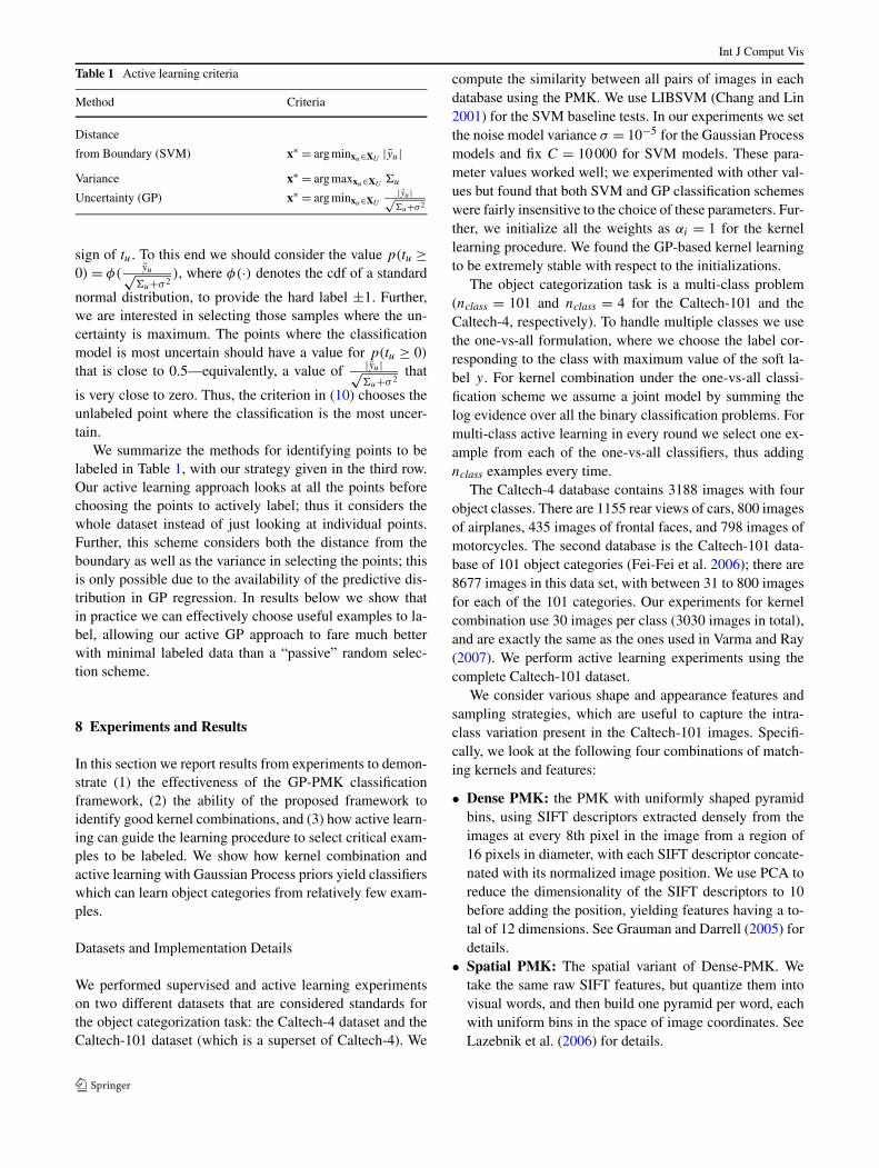
Table 1 Active learning criteria

Method Criteria

Distance

from Boundary (SVM) x∗ = arg minxu∈XU|yu|

Variance x∗ = arg maxxu∈XU�u

Uncertainty (GP) x∗ = arg minxu∈XU

|yu|√�u+σ 2

sign of tu. To this end we should consider the value p(tu ≥0) = φ(

yu√�u+σ 2

), where φ(·) denotes the cdf of a standard

normal distribution, to provide the hard label ±1. Further,we are interested in selecting those samples where the un-certainty is maximum. The points where the classificationmodel is most uncertain should have a value for p(tu ≥ 0)

that is close to 0.5—equivalently, a value of |yu|√�u+σ 2

that

is very close to zero. Thus, the criterion in (10) chooses theunlabeled point where the classification is the most uncer-tain.

We summarize the methods for identifying points to belabeled in Table 1, with our strategy given in the third row.Our active learning approach looks at all the points beforechoosing the points to actively label; thus it considers thewhole dataset instead of just looking at individual points.Further, this scheme considers both the distance from theboundary as well as the variance in selecting the points; thisis only possible due to the availability of the predictive dis-tribution in GP regression. In results below we show thatin practice we can effectively choose useful examples to la-bel, allowing our active GP approach to fare much betterwith minimal labeled data than a “passive” random selec-tion scheme.

8 Experiments and Results

In this section we report results from experiments to demon-strate (1) the effectiveness of the GP-PMK classificationframework, (2) the ability of the proposed framework toidentify good kernel combinations, and (3) how active learn-ing can guide the learning procedure to select critical exam-ples to be labeled. We show how kernel combination andactive learning with Gaussian Process priors yield classifierswhich can learn object categories from relatively few exam-ples.

Datasets and Implementation Details

We performed supervised and active learning experimentson two different datasets that are considered standards forthe object categorization task: the Caltech-4 dataset and theCaltech-101 dataset (which is a superset of Caltech-4). We

compute the similarity between all pairs of images in eachdatabase using the PMK. We use LIBSVM (Chang and Lin2001) for the SVM baseline tests. In our experiments we setthe noise model variance σ = 10−5 for the Gaussian Processmodels and fix C = 10 000 for SVM models. These para-meter values worked well; we experimented with other val-ues but found that both SVM and GP classification schemeswere fairly insensitive to the choice of these parameters. Fur-ther, we initialize all the weights as αi = 1 for the kernellearning procedure. We found the GP-based kernel learningto be extremely stable with respect to the initializations.

The object categorization task is a multi-class problem(nclass = 101 and nclass = 4 for the Caltech-101 and theCaltech-4, respectively). To handle multiple classes we usethe one-vs-all formulation, where we choose the label cor-responding to the class with maximum value of the soft la-bel y. For kernel combination under the one-vs-all classi-fication scheme we assume a joint model by summing thelog evidence over all the binary classification problems. Formulti-class active learning in every round we select one ex-ample from each of the one-vs-all classifiers, thus addingnclass examples every time.

The Caltech-4 database contains 3188 images with fourobject classes. There are 1155 rear views of cars, 800 imagesof airplanes, 435 images of frontal faces, and 798 images ofmotorcycles. The second database is the Caltech-101 data-base of 101 object categories (Fei-Fei et al. 2006); there are8677 images in this data set, with between 31 to 800 imagesfor each of the 101 categories. Our experiments for kernelcombination use 30 images per class (3030 images in total),and are exactly the same as the ones used in Varma and Ray(2007). We perform active learning experiments using thecomplete Caltech-101 dataset.

We consider various shape and appearance features andsampling strategies, which are useful to capture the intra-class variation present in the Caltech-101 images. Specifi-cally, we look at the following four combinations of match-ing kernels and features:

• Dense PMK: the PMK with uniformly shaped pyramidbins, using SIFT descriptors extracted densely from theimages at every 8th pixel in the image from a region of16 pixels in diameter, with each SIFT descriptor concate-nated with its normalized image position. We use PCA toreduce the dimensionality of the SIFT descriptors to 10before adding the position, yielding features having a to-tal of 12 dimensions. See Grauman and Darrell (2005) fordetails.

• Spatial PMK: The spatial variant of Dense-PMK. Wetake the same raw SIFT features, but quantize them intovisual words, and then build one pyramid per word, eachwith uniform bins in the space of image coordinates. SeeLazebnik et al. (2006) for details.

Int J Comput Vis

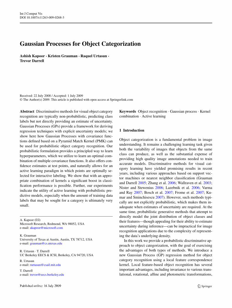
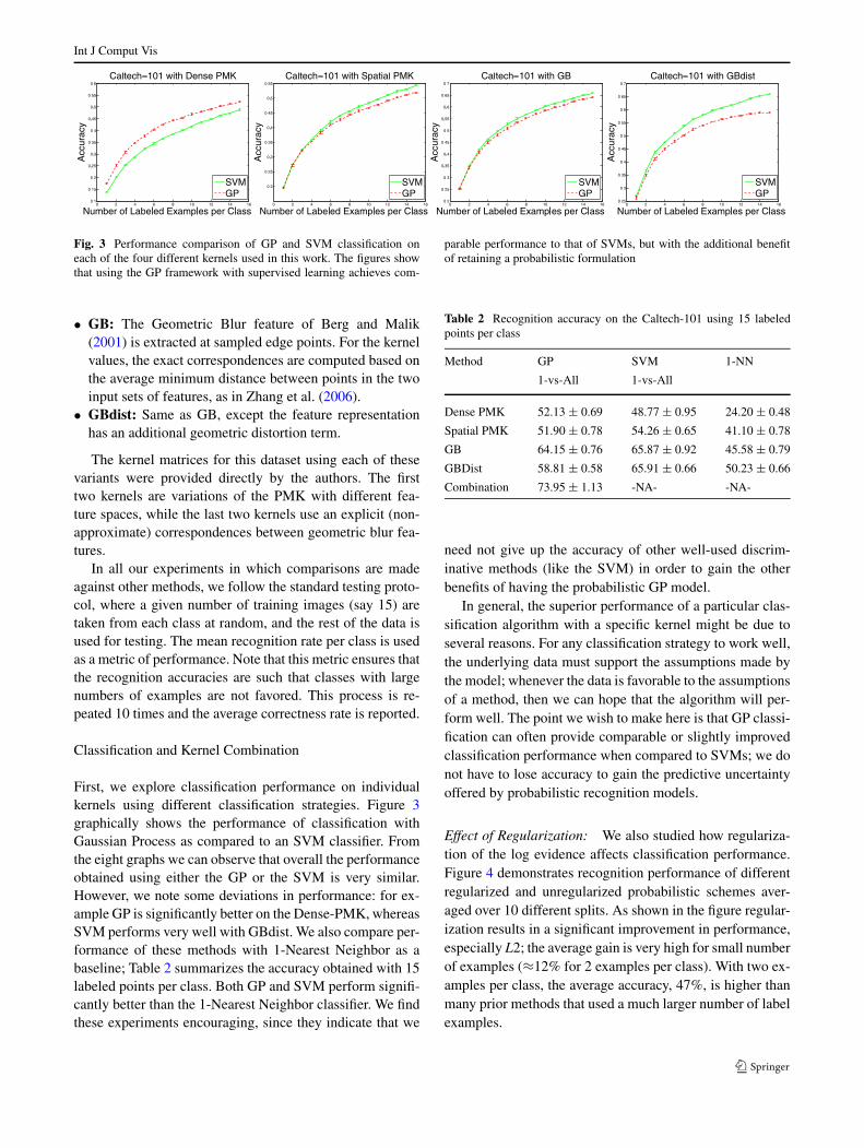
Fig. 3 Performance comparison of GP and SVM classification oneach of the four different kernels used in this work. The figures showthat using the GP framework with supervised learning achieves com-

parable performance to that of SVMs, but with the additional benefitof retaining a probabilistic formulation

• GB: The Geometric Blur feature of Berg and Malik(2001) is extracted at sampled edge points. For the kernelvalues, the exact correspondences are computed based onthe average minimum distance between points in the twoinput sets of features, as in Zhang et al. (2006).

• GBdist: Same as GB, except the feature representationhas an additional geometric distortion term.

The kernel matrices for this dataset using each of thesevariants were provided directly by the authors. The firsttwo kernels are variations of the PMK with different fea-ture spaces, while the last two kernels use an explicit (non-approximate) correspondences between geometric blur fea-tures.

In all our experiments in which comparisons are madeagainst other methods, we follow the standard testing proto-col, where a given number of training images (say 15) aretaken from each class at random, and the rest of the data isused for testing. The mean recognition rate per class is usedas a metric of performance. Note that this metric ensures thatthe recognition accuracies are such that classes with largenumbers of examples are not favored. This process is re-peated 10 times and the average correctness rate is reported.

Classification and Kernel Combination

First, we explore classification performance on individualkernels using different classification strategies. Figure 3graphically shows the performance of classification withGaussian Process as compared to an SVM classifier. Fromthe eight graphs we can observe that overall the performanceobtained using either the GP or the SVM is very similar.However, we note some deviations in performance: for ex-ample GP is significantly better on the Dense-PMK, whereasSVM performs very well with GBdist. We also compare per-formance of these methods with 1-Nearest Neighbor as abaseline; Table 2 summarizes the accuracy obtained with 15labeled points per class. Both GP and SVM perform signifi-cantly better than the 1-Nearest Neighbor classifier. We findthese experiments encouraging, since they indicate that we

Table 2 Recognition accuracy on the Caltech-101 using 15 labeledpoints per class

Method GP SVM 1-NN

1-vs-All 1-vs-All

Dense PMK 52.13 ± 0.69 48.77 ± 0.95 24.20 ± 0.48

Spatial PMK 51.90 ± 0.78 54.26 ± 0.65 41.10 ± 0.78

GB 64.15 ± 0.76 65.87 ± 0.92 45.58 ± 0.79

GBDist 58.81 ± 0.58 65.91 ± 0.66 50.23 ± 0.66

Combination 73.95 ± 1.13 -NA- -NA-

need not give up the accuracy of other well-used discrim-inative methods (like the SVM) in order to gain the otherbenefits of having the probabilistic GP model.

In general, the superior performance of a particular clas-sification algorithm with a specific kernel might be due toseveral reasons. For any classification strategy to work well,the underlying data must support the assumptions made bythe model; whenever the data is favorable to the assumptionsof a method, then we can hope that the algorithm will per-form well. The point we wish to make here is that GP classi-fication can often provide comparable or slightly improvedclassification performance when compared to SVMs; we donot have to lose accuracy to gain the predictive uncertaintyoffered by probabilistic recognition models.

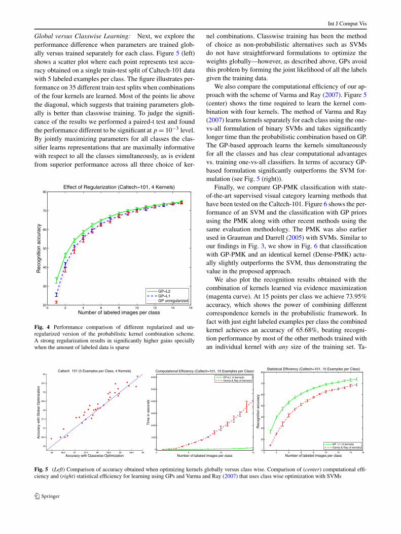
Effect of Regularization: We also studied how regulariza-tion of the log evidence affects classification performance.Figure 4 demonstrates recognition performance of differentregularized and unregularized probabilistic schemes aver-aged over 10 different splits. As shown in the figure regular-ization results in a significant improvement in performance,especially L2; the average gain is very high for small numberof examples (≈12% for 2 examples per class). With two ex-amples per class, the average accuracy, 47%, is higher thanmany prior methods that used a much larger number of labelexamples.

Int J Comput Vis

Global versus Classwise Learning: Next, we explore theperformance difference when parameters are trained glob-ally versus trained separately for each class. Figure 5 (left)shows a scatter plot where each point represents test accu-racy obtained on a single train-test split of Caltech-101 datawith 5 labeled examples per class. The figure illustrates per-formance on 35 different train-test splits when combinationsof the four kernels are learned. Most of the points lie abovethe diagonal, which suggests that training parameters glob-ally is better than classwise training. To judge the signifi-cance of the results we performed a paired-t test and foundthe performance different to be significant at p = 10−3 level.By jointly maximizing parameters for all classes the clas-sifier learns representations that are maximally informativewith respect to all the classes simultaneously, as is evidentfrom superior performance across all three choice of ker-

Fig. 4 Performance comparison of different regularized and un-regularized version of the probabilistic kernel combination scheme.A strong regularization results in significantly higher gains speciallywhen the amount of labeled data is sparse

nel combinations. Classwise training has been the methodof choice as non-probabilistic alternatives such as SVMsdo not have straightforward formulations to optimize theweights globally—however, as described above, GPs avoidthis problem by forming the joint likelihood of all the labelsgiven the training data.

We also compare the computational efficiency of our ap-proach with the scheme of Varma and Ray (2007). Figure 5(center) shows the time required to learn the kernel com-bination with four kernels. The method of Varma and Ray(2007) learns kernels separately for each class using the one-vs-all formulation of binary SVMs and takes significantlylonger time than the probabilistic combination based on GP.The GP-based approach learns the kernels simultaneouslyfor all the classes and has clear computational advantagesvs. training one-vs-all classifiers. In terms of accuracy GP-based formulation significantly outperforms the SVM for-mulation (see Fig. 5 (right)).

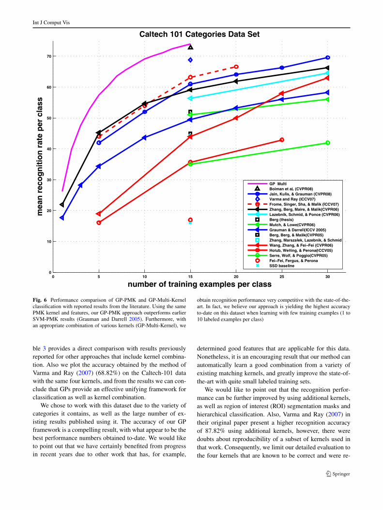
Finally, we compare GP-PMK classification with state-of-the-art supervised visual category learning methods thathave been tested on the Caltech-101. Figure 6 shows the per-formance of an SVM and the classification with GP priorsusing the PMK along with other recent methods using thesame evaluation methodology. The PMK was also earlierused in Grauman and Darrell (2005) with SVMs. Similar toour findings in Fig. 3, we show in Fig. 6 that classificationwith GP-PMK and an identical kernel (Dense-PMK) actu-ally slightly outperforms the SVM, thus demonstrating thevalue in the proposed approach.

We also plot the recognition results obtained with thecombination of kernels learned via evidence maximization(magenta curve). At 15 points per class we achieve 73.95%accuracy, which shows the power of combining differentcorrespondence kernels in the probabilistic framework. Infact with just eight labeled examples per class the combinedkernel achieves an accuracy of 65.68%, beating recogni-tion performance by most of the other methods trained withan individual kernel with any size of the training set. Ta-

Fig. 5 (Left) Comparison of accuracy obtained when optimizing kernels globally versus class wise. Comparison of (center) computational effi-ciency and (right) statistical efficiency for learning using GPs and Varma and Ray (2007) that uses class wise optimization with SVMs

Int J Comput Vis

Fig. 6 Performance comparison of GP-PMK and GP-Multi-Kernelclassification with reported results from the literature. Using the samePMK kernel and features, our GP-PMK approach outperforms earlierSVM-PMK results (Grauman and Darrell 2005). Furthermore, withan appropriate combination of various kernels (GP-Multi-Kernel), we

obtain recognition performance very competitive with the state-of-the-art. In fact, we believe our approach is yielding the highest accuracyto-date on this dataset when learning with few training examples (1 to10 labeled examples per class)

ble 3 provides a direct comparison with results previouslyreported for other approaches that include kernel combina-tion. Also we plot the accuracy obtained by the method ofVarma and Ray (2007) (68.82%) on the Caltech-101 datawith the same four kernels, and from the results we can con-clude that GPs provide an effective unifying framework forclassification as well as kernel combination.

We chose to work with this dataset due to the variety ofcategories it contains, as well as the large number of ex-isting results published using it. The accuracy of our GPframework is a compelling result, with what appear to be thebest performance numbers obtained to-date. We would liketo point out that we have certainly benefited from progressin recent years due to other work that has, for example,

determined good features that are applicable for this data.Nonetheless, it is an encouraging result that our method canautomatically learn a good combination from a variety ofexisting matching kernels, and greatly improve the state-of-the-art with quite small labeled training sets.

We would like to point out that the recognition perfor-mance can be further improved by using additional kernels,as well as region of interest (ROI) segmentation masks andhierarchical classification. Also, Varma and Ray (2007) intheir original paper present a higher recognition accuracyof 87.82% using additional kernels, however, there weredoubts about reproducibility of a subset of kernels used inthat work. Consequently, we limit our detailed evaluation tothe four kernels that are known to be correct and were re-

Int J Comput Vis

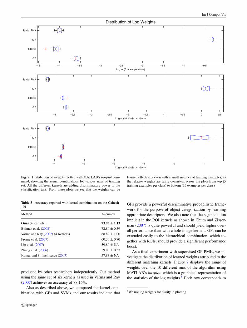
Fig. 7 Distribution of weights plotted with MATLAB’s boxplot com-mand, showing the kernel combinations for various sizes of trainingset. All the different kernels are adding discriminatory power to theclassification task. From these plots we see that the weights can be

learned effectively even with a small number of training examples, asthe relative weights are fairly consistent across the plots from top (5training examples per class) to bottom (15 examples per class)

Table 3 Accuracy reported with kernel combination on the Caltech-101

Method Accuracy

Ours (4 Kernels) 73.95 ± 1.13

Boiman et al. (2008) 72.80 ± 0.39

Varma and Ray (2007) (4 Kernels) 68.82 ± 1.00

Frome et al. (2007) 60.30 ± 0.70

Lin et al. (2007) 59.80 ± NA

Zhang et al. (2006) 59.08 ± 0.37

Kumar and Sminchisescu (2007) 57.83 ± NA

produced by other researchers independently. Our methodusing the same set of six kernels as used in Varma and Ray(2007) achieves an accuracy of 88.15%.

Also as described above, we compared the kernel com-bination with GPs and SVMs and our results indicate that

GPs provide a powerful discriminative probabilistic frame-work for the purpose of object categorization by learningappropriate descriptors. We also note that the segmentationimplicit in the ROI kernels as shown in Chum and Zisser-man (2007) is quite powerful and should yield higher over-all performance than with whole-image kernels. GPs can beextended easily to the hierarchical combination, which to-gether with ROIs, should provide a significant performanceboost.

As a final experiment with supervised GP-PMK, we in-vestigate the distribution of learned weights attributed to thedifferent matching kernels. Figure 7 displays the range ofweights over the 10 different runs of the algorithm usingMATLAB’s boxplot, which is a graphical representation ofthe statistics of the log weights.5 Each row corresponds to

5We use log weights for clarity in plotting.

Int J Comput Vis

a kernel, and the red line in each row denotes the medianover the 10 different runs. The end lines are at the lower andupper quartile values, and the outliers are data with valuesbeyond the ends of the whiskers. We show boxplots for runswith five, 10 and 15 training examples per class. From thefigure we see that this distribution is fairly similar for differ-ent sizes of training sets. This highlights that we can hopeto learn the kernel weights even with very few data points.Further, we also notice that the weight corresponding to thespatial PMK is often fairly high. However, we cannot inter-pret the weights directly as a measure of importance. This isdue to the fact that the scale of each kernel is different; thus,the weight encompasses both the discriminatory power aswell as automatic scale adjustment.

Finally, we would like to point out that the mean ac-curacy with a learned kernel combination using 15 train-ing examples per class over 10 random train-test splits was73.95% with a standard deviation of 1.13 (see Table 2).The low standard deviation value highlights the stability ofthe method’s classification accuracy with respect to the dataused to learn the weights. Moreover, in our experiments wefound that GP-based kernel combination (sum of weightedkernels) was extremely stable with respect to the initializa-tion. In fact, in all our experiments we perform the opti-mization only once (as opposed to optimizing with mul-tiple initializations). As expected, the classification accu-racy steadily increases as we increase the number of labeledpoints; however, the performance is very competitive evenwith small number of examples per class (for example GP-Multi-Kernel is better than most of the methods for 5 exam-ples per class).

Active Learning for Object Categorization

In this section, we show the value of active learning in se-lecting examples to annotate. For these experiments, we testthe classification performance on a validation set that in-cludes 10 examples from each class. We first consider thebinary problem of detecting an object class. Starting withone labeled example per class, the procedure chooses thenext image to query from the set of images not in the valida-tion set. We compare the active version of the GP classifica-tion with a version that selects the points to query randomly.We again use the mean classification rate per class to com-pare the methods. We repeat this procedure for 100 differentvalidation sets.

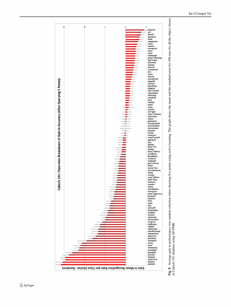
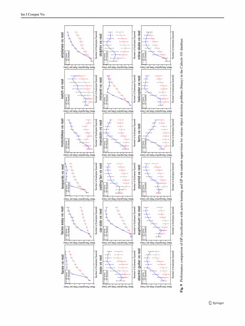
Figure 8 shows the gain in performance on all the 101binary problems, averaged over the 100 runs, made by theactive learning scheme on the validation set after 5 exam-ples are chosen. We can clearly see that for most of the cate-gories there is a significant positive gain showing the benefitof the active learning scheme. Further, Fig. 9 shows the per-formance on various binary problems as we increase the size

of the training set. The figure depicts that the active learningscheme quickly exploits the uncertainty in its estimates toselect appropriate examples to seek the annotation for. Therandom policy on the other hand performs poorly. The factthat the Caltech-101 dataset has unbalanced numbers of ex-amples per category affects the random sampling policy; itdoes not work well in these unbalanced scenarios becausethe training set will usually be skewed towards one class,resulting in poor accuracy. However, selecting points via ac-tive learning focuses on points with maximum uncertainty,irrespective of their label, making the procedure highly ef-fective.

Next we describe active learning experiments with theCaltech-4 dataset using multiple feature sampling and pyra-mid partitioning strategies. The goal here was to investigatethe benefits of the proposed scheme across the spectrum ofkernels available for the task of object categorization. Forthis experiment we again experimented with three differentflavors of the Pyramid Match Kernel. Besides Dense PMK,we also used PMK computed using only sparse interestpoints where salient points in the images are detected witha Harris-Affine interest operator (Harris PMK). The thirdPMK variant was vocabulary guided (Vocabulary GuidedPMK) where the features were binned non-uniformly in adata-dependent manner, as in Grauman and Darrell (2006a).

Figure 10 compares different classification approacheson the Caltech-4 database for different kinds of kernels. Es-sentially, the plot shows mean classification accuracy perclass as we vary the total number of examples in the trainingdata. The images not in the training set are considered as thetest set to compute the classification performance. We plotthe performance of the SVM and the GP classification withand without active learning. We start with one labeled pointper class. For the SVM and supervised GP without activelearning, we randomly select points as we increase the sizeof the training set, whereas for the active learning with GPclassification and SVM we used all the criteria mentionedin Table 1. This process was repeated 40 times. Figure 10shows the mean performance together with error bars denot-ing the standard error.

From Fig. 10 we observe that GP classification again per-forms competitively with SVM, and using active learningfurther improves the performance. Note that active learningusing uncertainty is superior to active learning using justvariance or just the classifier output (margin). The activelearning results that use only the variance are far inferiorto the other methods, mostly due to the fact that this variantof the criterion does not consider the class label of the datapoints already in the training set. A similar observation hasalso been made by Krause et al. (2008). On the other hand,the active learning criterion that uses uncertainty is effective.In fact we can see that a mean accuracy per class close to90% can be obtained with just 20 labeled examples, whereas

Int J Comput Vis

Fig

.8A

vera

gega

inin

perf

orm

ance

over

rand

omse

lect

ion

whe

nch

oosi

ngfiv

epo

ints

usin

gac

tive

lear

ning

.The

grap

hsh

ows

the

mea

nan

dth

est

anda

rder

ror

for

100

runs

for

allt

heob

ject

clas

ses

inC

alte

ch-1

01da

taba

seus

ing

GP-

PMK

Int J Comput Vis

Fig

.9Pe

rfor

man

ceco

mpa

riso

nof

GP

clas

sific

atio

nw

ithac

tive

lear

ning

and

GP

with

rand

omsu

perv

isio

nfo

rva

riou

sob

ject

dete

ctio

npr

oble

ms

(bin

ary)

inth

eC

alte

ch-1

01da

taba

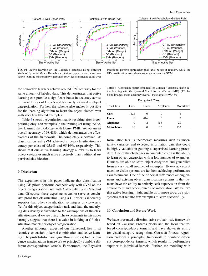
se

Int J Comput Vis

Fig. 10 Active learning on the Caltech-4 database using differentkinds of Pyramid Match Kernels and feature types. In each case, ouractive learning (uncertainty) approach provides significant gains over

traditional passive approaches that label points at random, while theGP classification even shows some gains over the SVM

the non-active learners achieve around 85% accuracy for thesame amount of labeled data. This demonstrates that activelearning can provide a significant boost in accuracy acrossdifferent flavors of kernels and feature types used in objectcategorization. Further, the scheme also makes it possiblefor the learning algorithm to learn the object classes evenwith very few labeled examples.

Table 4 shows the confusion matrix resulting after incor-porating only 120 examples in the training set using the ac-tive learning methodology with Dense PMK. We obtain anoverall accuracy of 98.48%, which demonstrates the effec-tiveness of the framework. The completely supervised GPclassification and SVM achieved a mean classification ac-curacy per class of 95.6% and 95.19%, respectively. Thisshows that our active learning strategy allows us to learnobject categories much more effectively than traditional su-pervised classification.

9 Discussion

The experiments in this paper indicate that classificationusing GP priors performs competitively with SVM on theobject categorization task with Caltech-101 and Caltech-4data. Of course, these experiments cannot serve as conclu-sive proof that classification using a GP prior is inherentlysuperior than other classification techniques or vice-versa.Yet for this object categorization task and data, the underly-ing data density is favorable to the assumptions of the clas-sification model we are using. The experiments in this paperstrongly suggest that there is a value in looking at GP clas-sification models for object categorization.

Another important aspect of our framework lies in itsseamless extension to kernel combination and active learn-ing. The probabilistic paradigm allows us to exploit the evi-dence maximization framework to principally combine dif-ferent correspondence kernels. Furthermore, the Bayesian

Table 4 Confusion matrix obtained for Caltech-4 database using ac-tive learning with the Pyramid Match Kernel (Dense PMK). (120 la-beled images, mean accuracy over all the classes = 98.48%)

Recognized Class

True Class Cars Faces Airplanes Motorbikes

Cars 1121 0 0 1

Faces 0 416 0 2

Airplanes 0 2 753 20

Motorbikes 10 0 10 733

formulation lets us incorporate measures such as uncer-tainty, variance, and expected information gain that couldbe highly valuable in guiding a supervised learning proce-dure. One of the challenges in computer vision is the abilityto learn object categories with a low number of examples.Humans are able to learn object categories and generalizefrom a very small number of examples. However, currentmachine vision systems are far from achieving performanceakin to humans. One of the principal differences among hu-mans and existing object classification systems is that hu-mans have the ability to actively seek supervision from theenvironment and other sources of information. We believethat active learning might enable us to move towards visionsystems that require few examples to learn successfully.

10 Conclusion and Future Work

We have presented a discriminative probabilistic frameworkbased on Gaussian Process priors and the local feature-based correspondence kernels, and have shown its utilityfor visual category recognition. Gaussian Process regres-sion provides a principled framework to combine differ-ent correspondence kernels, which results in performancesuperior to individual kernels. Further, the modeling with

Int J Comput Vis

Gaussian Process priors provides direct estimates of pre-diction uncertainty using a smoothness prior that capturesa correspondence-based notion of similarity between setsof local image features. We introduced an active learningmethod for visual category recognition based on the GP-PMK uncertainty estimates, and showed empirically that ac-tive learning can be used to achieve very good recognitionresults using far fewer training images than standard super-vised learning approaches.

We plan to extend the framework to adopt non-Gaussiannoise models, and investigate other active learning formula-tions such as value of information and/or criteria previouslydeveloped for sparsifying GPs (Lawrence et al. 2002). Byincorporating decision-theoretic formulations we should beable to learn object categories within a given budget. Wealso plan to extend the model to handle multiple objects inthe same image, incorporate semi-supervised learning, andexplore sparse GP techniques for large training sets.

Acknowledgements We thank the following for providing kernelmatrices: Alex Berg, Anna Bosch, Jitendra Malik and Andrew Zisser-man. We also wish to thank Manik Varma for his help in obtainingthe required data and for many helpful discussions. Kristen Graumanis supported in part by NSF CAREER award #0747356, a MicrosoftResearch New Faculty Fellowship, Texas Higher Education Coordinat-ing Board award #003658-01-40-2007, DARPA VIRAT, and the HenryLuce Foundation.

Open Access This article is distributed under the terms of the Cre-ative Commons Attribution Noncommercial License which permitsany noncommercial use, distribution, and reproduction in any medium,provided the original author(s) and source are credited.

References

Abramson, Y., & Freund, Y. (2004). Active learning for visual objectrecognition (Technical report). UCSD.

Belongie, S., Malik, J., & Puzicha, J. (2001). Matching shapes. InICCV.

Berg, A., & Malik, J. (2001). Geometric blur for template matching. InCVPR.

Boiman, O., Shechtman, E., & Irani, M. (2008). In defense of nearest-neighbor based image classification. In CVPR.

Bosch, A., Zisserman, A., & Muñoz, X. (2007). Representing shapewith a spatial pyramid kernel. In CIVR.

Chang, C., & Lin, C. (2001). LIBSVM: a library for SVMs.Chang, E. Y., Tong, S., Goh, K., & Chang, C. (2005). Support vector

machine concept-dependent active learning for image retrieval.IEEE Transactions on Multimedia.

Chum, O., & Zisserman, A. (2007). An exemplar model for learningobject classes. In Proceedings of the IEEE conference on com-puter vision and pattern recognition.

Evgeniou, T., Pontil, M., & Poggio, T. (2000). Regularization networksand support vector machines. Advances in Computational Mathe-matics, 13(1).

Fei-Fei, L., Fergus, R., & Perona, P. (2006). One-shot learning of ob-ject categories. IEEE Transaction on Pattern Recognition and Ma-chine Intelligence.

Fergus, R., Perona, P., & Zisserman, A. (2003). Object class recogni-tion by unsupervised scale-invariant learning. In CVPR.

Freund, Y., Seung, H. S., Shamir, E., & Tishby, N. (1997). Selec-tive sampling using the query by committee algorithm. MachineLearning, 28(2–3).

Frome, A., Singer, Y., Sha, F., & Malik, J. (2007). Learning globally-consistent local distance functions for shape-based image retrievaland classification. In ICCV.

Grauman, K., & Darrell, T. (2005). The pyramid match kernel: Dis-criminative classification with sets of image features. In ICCV.

Grauman, K., & Darrell, T. (2006a). Approximate correspondences inhigh dimensions. In NIPS.

Grauman, K., & Darrell, T. (2006b). Unsupervised learning of cate-gories from sets of partially matching image features. In CVPR.

Kadir, T., & Brady, M. (2003). Scale saliency: A novel approach tosalient feature and scale selection. In International conference vi-sual information engineering.

Kapoor, A., Grauman, K., Urtasun, R., & Darrell, T. (2007). Activelearning with Gaussian processes for object categorization. InICCV.

Kim, H. C., Kim, D., Ghahramani, Z., & Bang, S. Y. (2006).Appearance-based gender classification with Gaussian processes.Pattern Recognition Letters.

Krause, A., Singh, A., & Guestrin, C. (2008). Near-optimal sensorplacements in Gaussian processes: Theory, efficient algorithmsand empirical studies. In JMLR.

Kumar, A., & Sminchisescu, C. (2007). Support kernel machines forobject recognition. In ICCV.

Lawrence, N. (2004). Gaussian process latent variable models for vi-sualisation of high dimensional data. In NIPS.

Lawrence, N., Seeger, M., & Herbrich, R. (2002). Fast sparse Gaussianprocess method: Informative vector machines. In NIPS.

Lazebnik, S., Schmid, C., & Ponce, J. (2006). Beyond bags of fea-tures: Spatial pyramid matching for recognizing natural scene cat-egories. In CVPR.

Lin, Y. Y., Liu, T. Y., & Fuh, C. S. (2007). Local ensemble kernel learn-ing for object category recognition. In CVPR.

Lowe, D. (2004). Distinctive image features from scale-invariant key-points. IJCV, 60(2).

MacKay, D. (1992) Information-based objective functions for activedata selection. Neural Computation, 4(4).

McCallum, A. K., & Nigam, K. (1998). Employing EM in pool-basedactive learning for text classification. In ICML.

Mikolajczyk, K., & Schmid, C. (2001). Indexing based on scale invari-ant interest points. In ICCV.

Mikolajczyk, K., & Schmid, C. (2004). Scale and affine invariant in-terest point detectors. IJCV, 1(60), 63–86.

Minka, T. P. (2001). A family of algorithms for approximate Bayesianinference. PhD thesis, MIT.

Moosmann, B. T. F., & Jurie, F. (2007). Fast discriminative visual code-books using randomized clustering forests. In NIPS.

Muslea, I., Minton, S., & Knoblock, C. A. (2002). Active + semi-supervised learning = robust multi-view learning. In ICML.

Nister, D., & Stewenius, H. (2006). Scalable recognition with a vocab-ulary tree. In CVPR.

Nowak, E., Jurie, F., & Triggs, B. (2006). Sampling strategies for bag-of-features image classification. In ECCV.

Rasmusen, C. E., & Williams, C. (2006). Gaussian processes for ma-chine learning. Cambridge: MIT Press.

Seeger, M. (2004). Gaussian processes for machine learning. Interna-tional Journal of Neural Systems, 14(2).

Shen, Y., Ng, A., & Seeger, M. (2006). Fast Gaussian process regres-sion using kd-trees. In NIPS.

Sivic, J., & Zisserman, A. (2003). Video Google: a text retrieval ap-proach to object matching in videos. In ICCV.

Sivic, J., Russell, B., Efros, A., Zisserman, A., & Freeman, W. (2005).Discovering object categories in image collections. In ICCV.

Snelson, E., & Ghahramani, Z. (2006). Sparse Gaussian processes us-ing pseudo-inputs. In NIPS.

Int J Comput Vis

Sudderth, E., Torralba, A., Freeman, W., & Willsky, A. (2005). De-scribing visual scenes using transformed Dirichlet processes. InNIPS.

Tong, S., & Koller, D. (2000). Support vector machine active learningwith applications to text classification. In ICML.

Tresp, V. (2000). Mixtures of Gaussian processes. In NIPS.Tsang, I. W.-H., & Kwok, J. T.-Y. (2006). Efficient hyperkernel learn-

ing using second-order cone programming. IEEE Transactions onNeural Networks.

Urtasun, R., & Darrell, T. (2008). Local probabilistic regression foractivity-independent human pose inference. In CVPR.

Urtasun, R., Fleet, D. J., Hertzman, A., & Fua, P. (2005). Priors forpeople tracking from small training sets. In ICCV.

Urtasun, R., Fleet, D. J., & Fua, P. (2006). Gaussian process dynamicalmodels for 3d people tracking. In CVPR.

Varma, M., & Ray, D. (2007). Learning the discriminative power-invariance trade-off. In ICCV.

von Ahn, L., & Dabbish, L. (2004). Labeling images with a computergame. In ACM CHI.

von Ahn, L., Liu, R., & Blum, M. (2006). Peekaboom: A game forlocating objects in images. In ACM CHI.

Wallraven, C., Caputo, B., & Graf, A. (2003). Recognition with localfeatures: the kernel recipe. In ICCV.

Williams, C., & Barber, D. (1998). Bayesian classification withGaussian processes. IEEE Transaction on Pattern Recognitionand Machine Intelligence, 20(12), 1342–1351.

Williams, O. (2006). A switched Gaussian process for estimating dis-parity and segmentation in binocular stereo. In NIPS.

Zhang, H., Berg, A., Maire, M., & Malik, J. (2006). SVM-KNN:Discriminative nearest neighbor classification for visual categoryrecognition. In CVPR.

Zhu, X., Lafferty, J., & Ghahramani, Z. (2003). Combining activelearning and semi-supervised learning using Gaussian fields andharmonic functions. In Workshop on the continuum from labeledto unlabeled data in machine learning and data mining at ICML.