Embed Size (px)
Citation preview

Gaussian Mixture Models (GMM)
and the K-Means Algorithm
Source Material for Lecture
http://www.autonlab.org/tutorials/gmm.html
http://research.microsoft.com/~cmbishop/talks.htm
Copyright © 2001, Andrew W. Moore
Very important in math and science due to the Central Limit Theorem: the distribution of the sum/mean of a set of iid random variables tends towards Gaussian as the number N of variables increases.
Example: sample mean of a set of N iid uniform(0,1) random variables:
N=1 N=2 N=10
Example: binomial distribution as a function of m (number of heads) ofN iid binary Bernoulli trials becomes more-and-more Gaussian-like for large N
Gaussian Distribution aka Multivariate Normal Distribution. Gaussian Distribution aka Multivariate Normal Distribution.
1 dimensional case
D dimensional case
mean
variance
mean vector
covariance matrix
Review: The Gaussian Distribution
• Multivariate Gaussian
mean covariance
Isotropic (circularly symmetric) if covariance is diag(k,k,...,k)
Gaussianconsider 2D case: constant-probability curves are ellipses
* centered at mean location u = (x0,y0)* oriented and elongated according to eigenvalues and
unit eigenvectors v of 2x2 symmetric pos.def. covariance matrix C
mean
max vmax
min vmin
special cases
C = diag(1, 2)axis-orientedellipses
C = circular(isotropic)
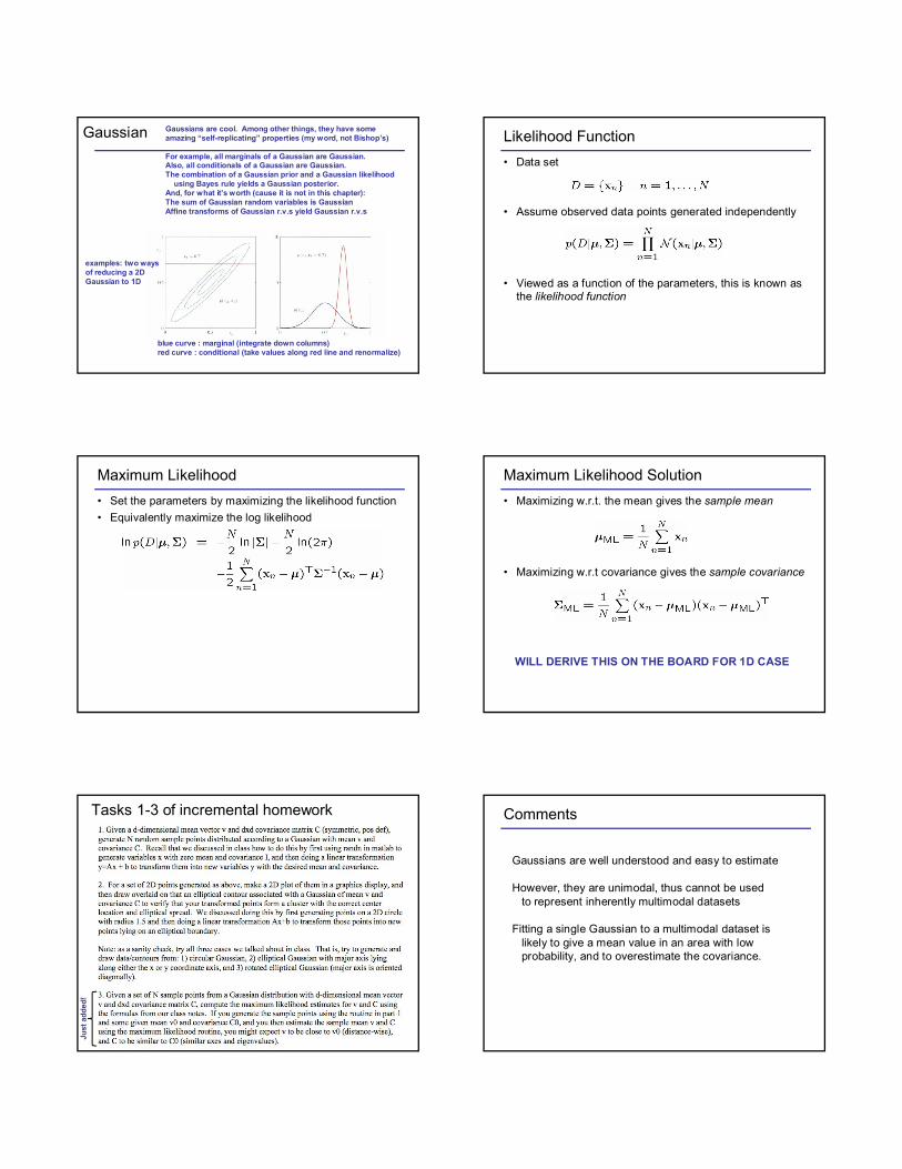
Gaussian Gaussians are cool. Among other things, they have someamazing “self-replicating” properties (my word, not Bishop’s)
For example, all marginals of a Gaussian are Gaussian.Also, all conditionals of a Gaussian are Gaussian.The combination of a Gaussian prior and a Gaussian likelihood
using Bayes rule yields a Gaussian posterior.And, for what it’s worth (cause it is not in this chapter):The sum of Gaussian random variables is GaussianAffine transforms of Gaussian r.v.s yield Gaussian r.v.s
blue curve : marginal (integrate down columns)red curve : conditional (take values along red line and renormalize)
examples: two waysof reducing a 2D Gaussian to 1D
Likelihood Function
• Data set
• Assume observed data points generated independently
• Viewed as a function of the parameters, this is known as the likelihood function
Maximum Likelihood
• Set the parameters by maximizing the likelihood function
• Equivalently maximize the log likelihood
Maximum Likelihood Solution
• Maximizing w.r.t. the mean gives the sample mean
• Maximizing w.r.t covariance gives the sample covariance
WILL DERIVE THIS ON THE BOARD FOR 1D CASE
Tasks 1-3 of incremental homework
Just
ad
ded
!
Comments
Gaussians are well understood and easy to estimate
However, they are unimodal, thus cannot be usedto represent inherently multimodal datasets
Fitting a single Gaussian to a multimodal dataset islikely to give a mean value in an area with lowprobability, and to overestimate the covariance.

Old Faithful Data Set
Duration of eruption (minutes)
Time betweeneruptions (minutes)
Multi-Modal DataMajor problem with the Gaussian is that it can onlydescribe a distribution with one mode (one “bump”)
Bad description of bimodal data usingthe inherently unimodal Gaussian
However, if we are willing to use more thanone Gaussian, we can fit one to eachmode or cluster of the data.
Some Bio Assay data
some axis
som
e o
ther
ax
is
Sometimes it may noteven be easy to tell how many “bumps”there are…
Idea: Use a Mixture of Gaussians
• Linear super-position of Gaussians
• Normalization and positivity require
• Can interpret the mixing coefficients as prior probabilities
Mixture of Gaussians
mixture of 3 one-dimensionalNormal distributions
mixture of 3 two-dimensional Gaussians
GMM describing assay data
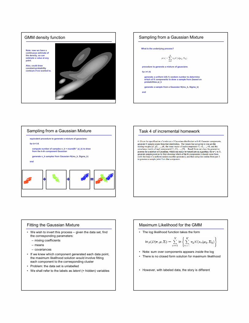
GMM density function
Note: now we have a continuous estimate of the density, so can estimate a value at any point.
Also, could draw constant-probability contours if we wanted to.
What is the underlying process?
procedure to generate a mixture of gaussians
for i=1:N
generate a uniform U(0,1) random number to determinewhich of K components to draw a sample from (based onprobabilities pi_k
generate a sample from a Gaussian N(mu_k, Sigma_k)
end
Sampling from a Gaussian Mixture
equivalent procedure to generate a mixture of gaussians:
for k=1:K
compute number of samples n_k = round(N * pi_k) to draw from the k-th component Gaussian
generate n_k samples from Gaussian N(mu_k, Sigma_k)
end
+ + =
Sampling from a Gaussian Mixture Task 4 of incremental homework
Fitting the Gaussian Mixture
• We wish to invert this process – given the data set, find the corresponding parameters:
– mixing coefficients
– means
– covariances
• If we knew which component generated each data point, the maximum likelihood solution would involve fitting each component to the corresponding cluster
• Problem: the data set is unlabelled
• We shall refer to the labels as latent (= hidden) variables
Maximum Likelihood for the GMM
• The log likelihood function takes the form
• Note: sum over components appears inside the log
• There is no closed form solution for maximum likelihood
• However, with labeled data, the story is different
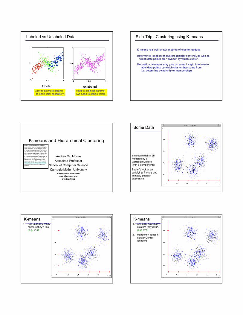
Labeled vs Unlabeled Data
labeled unlabeledEasy to estimate params(do each color separately)
Hard to estimate params(we need to assign colors)
Side-Trip : Clustering using K-means
K-means is a well-known method of clustering data.
Determines location of clusters (cluster centers), as well as which data points are “owned” by which cluster.
Motivation: K-means may give us some insight into how tolabel data points by which cluster they come from (i.e. determine ownership or membership)
K-means and Hierarchical Clustering
Andrew W. Moore
Associate Professor
School of Computer Science
Carnegie Mellon Universitywww.cs.cmu.edu/~awm
412-268-7599
Note to other teachers and users of these slides. Andrew would be delighted if you found this source material useful in giving your own lectures. Feel free to use these slides verbatim, or to modify them to fit your own needs. PowerPoint originals are available. If you make use of a significant portion of these slides in your own lecture, please include this message, or the following link to the source repository of Andrew’s tutorials: http://www.cs.cmu.edu/~awm/tutorials . Comments and corrections gratefully received.
Some Data
This could easily be modeled by a Gaussian Mixture (with 5 components)
But let’s look at an satisfying, friendly and infinitely popular alternative…
K-means1. Ask user how many
clusters they’d like. (e.g. k=5)
K-means1. Ask user how many
clusters they’d like. (e.g. k=5)
2. Randomly guess k cluster Center locations
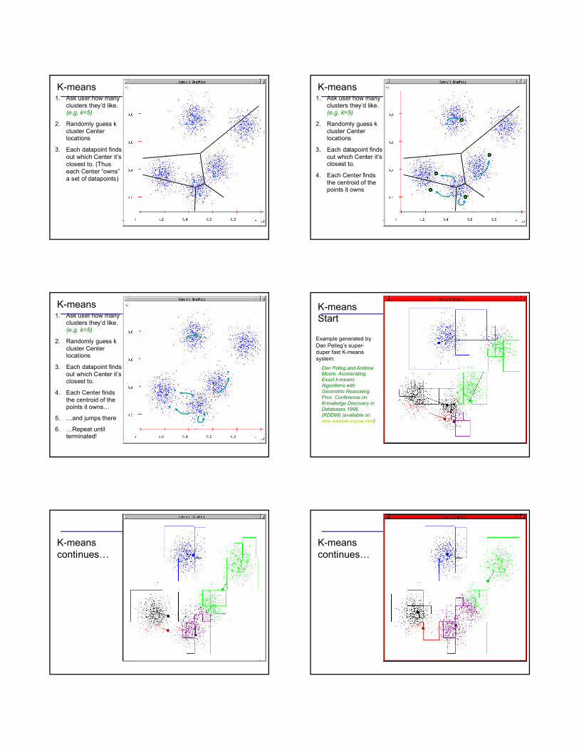
K-means1. Ask user how many
clusters they’d like. (e.g. k=5)
2. Randomly guess k cluster Center locations
3. Each datapoint finds out which Center it’s closest to. (Thus each Center “owns”a set of datapoints)
K-means1. Ask user how many
clusters they’d like. (e.g. k=5)
2. Randomly guess k cluster Center locations
3. Each datapoint finds out which Center it’s closest to.
4. Each Center finds the centroid of the points it owns
K-means1. Ask user how many
clusters they’d like. (e.g. k=5)
2. Randomly guess k cluster Center locations
3. Each datapoint finds out which Center it’s closest to.
4. Each Center finds the centroid of the points it owns…
5. …and jumps there
6. …Repeat until terminated!
K-means Start
Example generated by Dan Pelleg’s super-duper fast K-means system:
Dan Pelleg and Andrew Moore. Accelerating Exact k-means Algorithms with Geometric Reasoning. Proc. Conference on Knowledge Discovery in Databases 1999, (KDD99) (available on www.autonlab.org/pap.html)
K-means continues…
K-means continues…
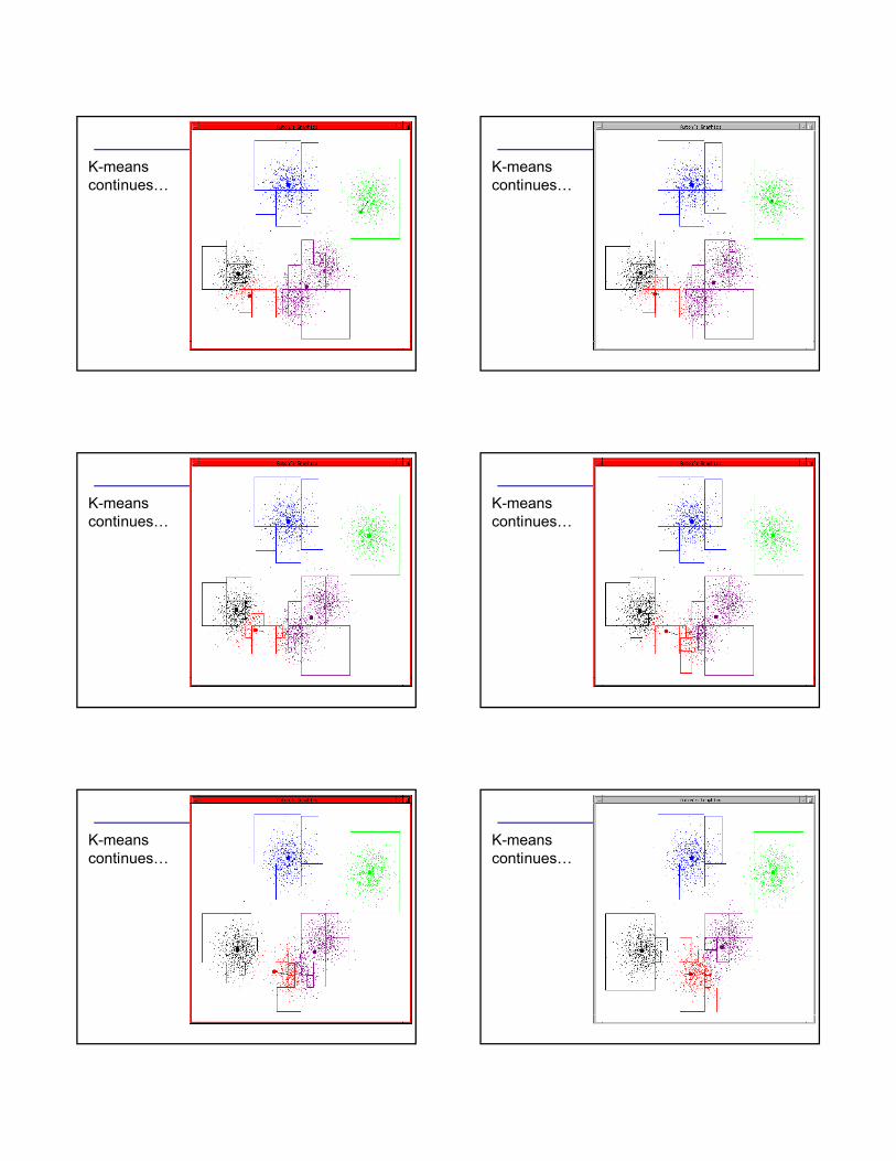
K-means continues…
K-means continues…
K-means continues…
K-means continues…
K-means continues…
K-means continues…
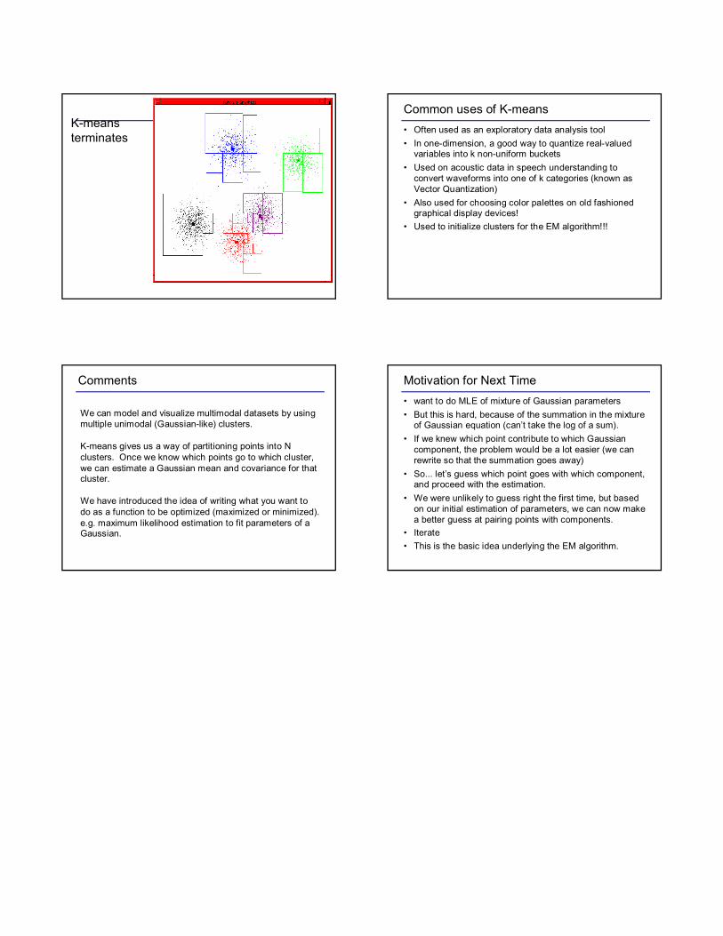
K-means terminates
Common uses of K-means
• Often used as an exploratory data analysis tool
• In one-dimension, a good way to quantize real-valued variables into k non-uniform buckets
• Used on acoustic data in speech understanding to convert waveforms into one of k categories (known as Vector Quantization)
• Also used for choosing color palettes on old fashioned graphical display devices!
• Used to initialize clusters for the EM algorithm!!!
Comments
We can model and visualize multimodal datasets by using multiple unimodal (Gaussian-like) clusters.
K-means gives us a way of partitioning points into N clusters. Once we know which points go to which cluster, we can estimate a Gaussian mean and covariance for that cluster.
We have introduced the idea of writing what you want to do as a function to be optimized (maximized or minimized). e.g. maximum likelihood estimation to fit parameters of a Gaussian.
Motivation for Next Time
• want to do MLE of mixture of Gaussian parameters
• But this is hard, because of the summation in the mixture of Gaussian equation (can’t take the log of a sum).
• If we knew which point contribute to which Gaussian component, the problem would be a lot easier (we can rewrite so that the summation goes away)
• So... let’s guess which point goes with which component, and proceed with the estimation.
• We were unlikely to guess right the first time, but based on our initial estimation of parameters, we can now make a better guess at pairing points with components.
• Iterate
• This is the basic idea underlying the EM algorithm.