Lecture notes Particle Physics II

Quantum Chromo Dynamics

3. U(1) Local Gauge Invariance

Michiel BotjeNikhef, Science Park, Amsterdam

November 16, 2013

Electric charge conservation

• In subatomic physics it is customary to express electric charge inunits of the elementary charge e = 1.6⇥ 10�19 Coulomb. Theelectron then has charge �1, the positron +1, the up quark +2

3,the down quark �1

3, etc., see the table on Page 1–5.

• As far as we know, total electric charge is the same in the ini-tial and final state of any elementary reaction, and this chargeconservation is experimentally verified to great accuracy.

• For instance electron decay

e ! � ⌫e

is allowed by all known conservation laws but is forbidden by chargeconservation and it indeed has never been observed. In fact, thelife time of the electron is measured to be larger than 5⇥1026 years.

• We have seen that conserved quantities are related to symmetriesin the Hamiltonian, or the Lagrangian, so the question is now whichsymmetry causes this charge conservation. Charge is obviously anadditive conserved quantity so that the symmetry transformationmust be continuous.

• The answer, as we will see, is that a so-called gauge symmetryis responsible for the charge conservation. Gauge transformationsenter when interactions are described in terms of potentials, insteadof forces. A well known example is from classical electrodynamicswhere we can transform the scalar and vector potentials in such away that the E and B fields are una↵ected.

3–3

Gauge transformation in electrodynamics

• In electrodynamics the E and B fields are related to the scalarand vector potentials V and A by

E = �@A/@t � rV B = r ⇥ A

• A gauge transformation leaves the E and B fields invariant

V 0 = V � @⇤/@t A

0 = A + r⇤

Here ⇤(x, t) is an arbitrary function of x and t.

• To this gauge transformation corresponds a unitary operator thattransforms the wave function of a particle in an electromagneticfield. We can write this transformation as (see page 2–7)

| i0 = exp(i✏G)| i

where the generator G is to be identified later. Since ⇤ is anarbitrary function of x and t we require that ✏ is also an arbitraryfunction of x and t. Because ✏ can vary in space-time, we speakof a local gauge transformation.

• Now consider the Schrodinger equation of a particle in a staticelectric field before and after our gauge transformation

i@| i@t

=

✓�r2

2m+ q V

◆| i

i@| i0

@t=

✓�r2

2m+ q V 0

◆| i0

Here q is the charge of the particle.

• Because of gauge invariance, both equations should apply andthis fixes the generator G, as we will now show.

3–4

From local gauge invariance to charge conservation

• Let us work out the transformed Schrodinger equation (for claritywe write instead of | i). To simplify the mathematics we willtake ✏ to be a function of t only, instead of x and t:

i@

@t

�ei✏G

�=

✓�r2

2m+ q V � q

@✏

@t

◆ei✏G

iei✏G

✓iG

@✏

@t+@

@t

◆= ei✏G

✓�r2

2m+ q V

◆ � ei✏G q

@✏

@t

�ei✏G G @✏

@t+ iei✏G @

@t= iei✏G @

@t� ei✏G q

@✏

@t

�ei✏G G @✏

@t= �ei✏G q

@✏

@t

G = q

• We find that G is the charge operator Q! This is due to thecancellations that occur because ✏ is local (i.e. a function of t inour derivation); all this would not work if ✏ would be a constant.

• Clearly if H and Q commute, then it follows that the expectationvalue hQi is conserved, in other words, charge is conserved.

• It is straight-forward to extend the derivation above to local trans-formations that depend on both x and t, instead of on t alone, butwe will not do this here since it brings a lot of additional algebraand is not very illuminating.

• The family of phase transformations U(↵) ⌘ ei↵, with real ↵,forms a unitary Abelian group called U(1). Phase invariance istherefore also known as U(1) invariance.

3–5

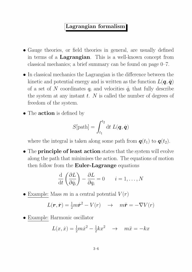
Lagrangian formalism

• Gauge theories, or field theories in general, are usually definedin terms of a Lagrangian. This is a well-known concept fromclassical mechanics; a brief summary can be found on page 0–7.

• In classical mechanics the Lagrangian is the di↵erence between thekinetic and potential energy and is written as the function L(q, q)of a set of N coordinates qi and velocities qi that fully describethe system at any instant t. N is called the number of degrees offreedom of the system.

• The action is defined by

S[path] =

Z t2

t1

dt L(q, q)

where the integral is taken along some path from q(t1) to q(t2).

• The principle of least action states that the system will evolvealong the path that minimises the action. The equations of motionthen follow from the Euler-Lagrange equations

d

dt

✓@L

@qi

◆� @L

@qi= 0 i = 1, . . . , N

• Example: Mass m in a central potential V (r)

L(r, r) = 12mr

2 � V (r) ! mr = �rV (r)

• Example: Harmonic oscillator

L(x, x) = 12mx2 � 1

2kx2 ! mx = �kx

3–6

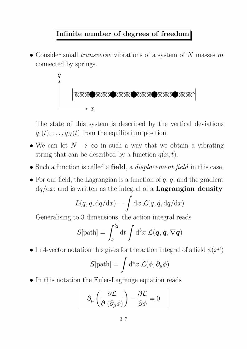
Infinite number of degrees of freedom

• Consider small transverse vibrations of a system of N masses mconnected by springs.

~ ~ ~ ~ ~QPPPPPPR QPPPPPPR QPPPPPPR QPPPPPPR QPPPPPPR QPPPPPPR-

6

q

x

The state of this system is described by the vertical deviationsq1(t), . . . , qN(t) from the equilibrium position.

• We can let N ! 1 in such a way that we obtain a vibratingstring that can be described by a function q(x, t).

• Such a function is called a field, a displacement field in this case.

• For our field, the Lagrangian is a function of q, q, and the gradientdq/dx, and is written as the integral of a Lagrangian density

L(q, q, dq/dx) =

Zdx L(q, q, dq/dx)

Generalising to 3 dimensions, the action integral reads

S[path] =

Z t2

t1

dt

Zd3x L(q, q,rq)

• In 4-vector notation this gives for the action integral of a field �(xµ)

S[path] =

Zd4x L(�, @µ�)

• In this notation the Euler-Lagrange equation reads

@µ

✓@L

@ (@µ�)

◆� @L@�

= 0

3–7

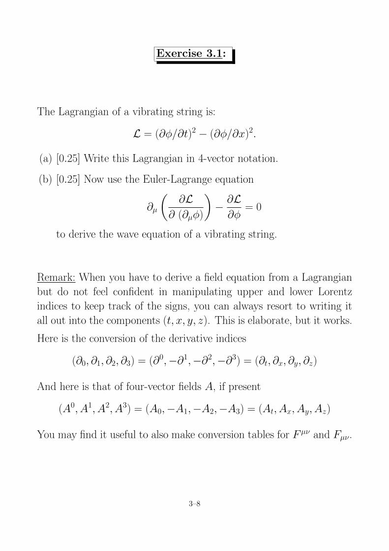
Exercise 3.1:

The Lagrangian of a vibrating string is:

L = (@�/@t)2 � (@�/@x)2.

(a) [0.25] Write this Lagrangian in 4-vector notation.

(b) [0.25] Now use the Euler-Lagrange equation

@µ

✓@L

@ (@µ�)

◆� @L@�

= 0

to derive the wave equation of a vibrating string.

Remark: When you have to derive a field equation from a Lagrangianbut do not feel confident in manipulating upper and lower Lorentzindices to keep track of the signs, you can always resort to writing itall out into the components (t, x, y, z). This is elaborate, but it works.

Here is the conversion of the derivative indices

(@0, @1, @2, @3) = (@0,�@1,�@2,�@3) = (@t, @x, @y, @z)

And here is that of four-vector fields A, if present

(A0, A1, A2, A3) = (A0,�A1,�A2,�A3) = (At, Ax, Ay, Az)

You may find it useful to also make conversion tables for Fµ⌫ and Fµ⌫.

3–8

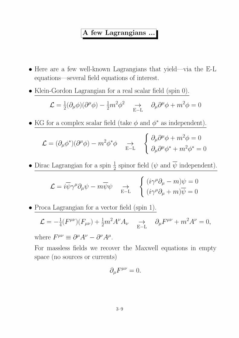
A few Lagrangians ...

• Here are a few well-known Lagrangians that yield—via the E-Lequations—several field equations of interest.

• Klein-Gordon Lagrangian for a real scalar field (spin 0).

L = 12(@µ�)(@

µ�) � 12m

2�2 !E�L

@µ@µ� +m2� = 0

• KG for a complex scalar field (take � and �⇤ as independent).

L = (@µ�⇤)(@µ�) � m2�⇤� !

E�L

(@µ@µ� +m2� = 0

@µ@µ�⇤ +m2�⇤ = 0

• Dirac Lagrangian for a spin 12 spinor field ( and independent).

L = i �µ@µ � m !E�L

((i�µ@µ � m) = 0

(i�µ@µ +m) = 0

• Proca Lagrangian for a vector field (spin 1).

L = �14(F

µ⌫)(Fµ⌫) +12m

2A⌫A⌫ !E�L

@µFµ⌫ +m2A⌫ = 0,

where Fµ⌫ ⌘ @µA⌫ � @⌫Aµ.

For massless fields we recover the Maxwell equations in emptyspace (no sources or currents)

@µFµ⌫ = 0.

3–9

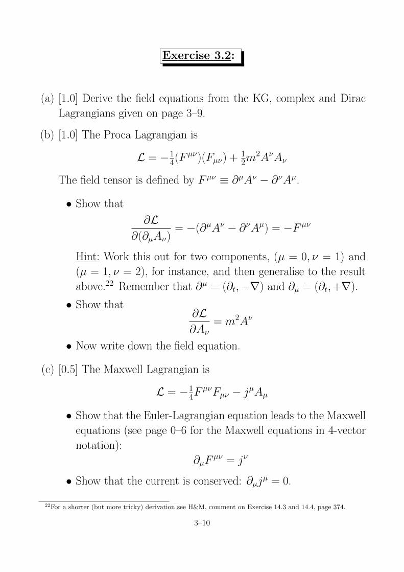
Exercise 3.2:

(a) [1.0] Derive the field equations from the KG, complex and DiracLagrangians given on page 3–9.

(b) [1.0] The Proca Lagrangian is

L = �14(F

µ⌫)(Fµ⌫) +12m

2A⌫A⌫

The field tensor is defined by Fµ⌫ ⌘ @µA⌫ � @⌫Aµ.

• Show that

@L@(@µA⌫)

= �(@µA⌫ � @⌫Aµ) = �Fµ⌫

Hint: Work this out for two components, (µ = 0, ⌫ = 1) and(µ = 1, ⌫ = 2), for instance, and then generalise to the resultabove.22 Remember that @µ = (@t,�r) and @µ = (@t,+r).

• Show that@L@A⌫

= m2A⌫

• Now write down the field equation.

(c) [0.5] The Maxwell Lagrangian is

L = �14F

µ⌫Fµ⌫ � jµAµ

• Show that the Euler-Lagrangian equation leads to the Maxwellequations (see page 0–6 for the Maxwell equations in 4-vectornotation):

@µFµ⌫ = j⌫

• Show that the current is conserved: @µjµ = 0.

22For a shorter (but more tricky) derivation see H&M, comment on Exercise 14.3 and 14.4, page 374.

3–10

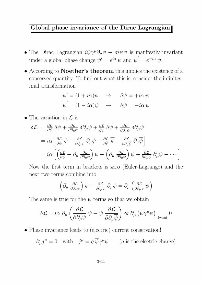
Global phase invariance of the Dirac Lagrangian

• The Dirac Lagrangian i �µ@µ � m is manifestly invariant

under a global phase change 0 = ei↵ and 0= e�i↵ .

• According toNoether’s theorem this implies the existence of aconserved quantity. To find out what this is, consider the infinites-imal transformation

0 = (1 + i↵) ! � = +i↵

0= (1 � i↵) ! � = �i↵

• The variation in L is

�L = @L@ � + @L

@@µ �@µ + @L

@ � + @L

@@µ �@µ

= i↵h@L@ + @L

@@µ @µ � @L

@ � @L

@@µ @µ

i

= i↵h⇣

@L@ � @µ

@L@@µ

⌘ +

⇣@µ

@L@@µ

⌘ + @L

@@µ @µ � · · ·

i

Now the first term in brackets is zero (Euler-Lagrange) and thenext two terms combine into

⇣@µ

@L@@µ

⌘ + @L

@@µ @µ = @µ

⇣@L@@µ

⌘

The same is true for the terms so that we obtain

�L = i↵ @µ

✓@L@@µ

� @L@@µ

◆/ @µ

� �µ

�=

Iwant0

• Phase invariance leads to (electric) current conservation!

@µjµ = 0 with jµ = q �µ (q is the electric charge)

3–11

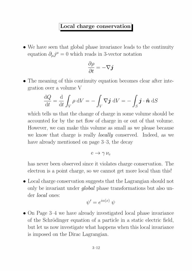
Local charge conservation

• We have seen that global phase invariance leads to the continuityequation @µjµ = 0 which reads in 3-vector notation

@⇢

@t= �rj

• The meaning of this continuity equation becomes clear after inte-gration over a volume V

dQ

dt=

d

dt

Z

V⇢ dV = �

Z

Vrj dV = �

Z

Sj · n dS

which tells us that the change of charge in some volume should beaccounted for by the net flow of charge in or out of that volume.However, we can make this volume as small as we please becausewe know that charge is really locally conserved. Indeed, as wehave already mentioned on page 3–3, the decay

e ! � ⌫e

has never been observed since it violates charge conservation. Theelectron is a point charge, so we cannot get more local than this!

• Local charge conservation suggests that the Lagrangian should notonly be invariant under global phase transformations but also un-der local ones:

0 = ei↵(x)

• On Page 3–4 we have already investigated local phase invarianceof the Schrodinger equation of a particle in a static electric field,but let us now investigate what happens when this local invarianceis imposed on the Dirac Lagrangian.

3–12

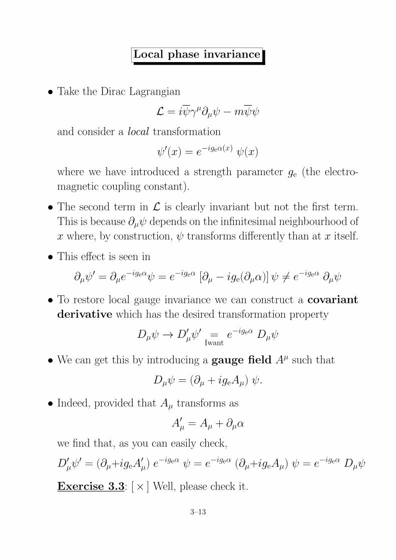
Local phase invariance

• Take the Dirac Lagrangian

L = i �µ@µ � m

and consider a local transformation

0(x) = e�ige↵(x) (x)

where we have introduced a strength parameter ge (the electro-magnetic coupling constant).

• The second term in L is clearly invariant but not the first term.This is because @µ depends on the infinitesimal neighbourhood ofx where, by construction, transforms di↵erently than at x itself.

• This e↵ect is seen in

@µ 0 = @µe

�ige↵ = e�ige↵ [@µ � ige(@µ↵)] 6= e�ige↵ @µ

• To restore local gauge invariance we can construct a covariantderivative which has the desired transformation property

Dµ ! D0µ

0 =Iwant

e�ige↵ Dµ

• We can get this by introducing a gauge field Aµ such that

Dµ = (@µ + igeAµ) .

• Indeed, provided that Aµ transforms as

A0µ = Aµ + @µ↵

we find that, as you can easily check,

D0µ

0 = (@µ+igeA0µ) e

�ige↵ = e�ige↵ (@µ+igeAµ) = e�ige↵ Dµ

Exercise 3.3: [⇥ ] Well, please check it.

3–13

Locally invariant Dirac Lagrangian

• So we can now propose, as a first step, the Lagrangian

L = i �µDµ � m = i �µ@µ � m | {z }

free term

� ge( �µ )Aµ| {z }

interaction term

which is invariant under local phase transformations and has ac-quired an interaction term jµAµ in addition to the free Lagrangian.

• We have a free term for the Dirac field, which suggests that weshould add a free term (Proca Lagrangian) for the gauge field Aµ

L = �14(F

µ⌫)(Fµ⌫) +12m

2A⌫A⌫

• Exercise 3.4: [0.5] Check that the first term is invariant underthe gauge transformation A0

µ = Aµ+@µ↵ but not the second term.

• To maintain gauge invariance we are thus forced to set m = 0 andconsider only a massless gauge field which, of course, turns out tobe the electromagnetic (photon) field.

• We have, in fact, found here a restriction that also applies tothe SU(2) and SU(3) gauge invariant Lagrangians that we willconsider later on:

To maintain gauge invariance, the gauge fieldmust be massless

3–14

The Lagrangian of QED

• We now can write-down the QED Lagrangian describing the inter-action of Dirac particles with the electromagnetic field

LQED = (iD/ � m) � 14(F

µ⌫)(Fµ⌫)

= (i@/ � m) � ge( �µ )Aµ � 1

4(Fµ⌫)(Fµ⌫)

In the expression above, we have introduced the usual shorthands@/ ⌘ �µ@µ = �µ@µ and D/ ⌘ �µDµ = �µDµ.

• Note that the last two terms in the QED Lagrangian correspondto Maxwell Lagrangian

LMaxwell = �14F

µ⌫Fµ⌫ � jµAµ

• This Lagrangian leads to the Maxwell equations (see Exercise 3.2)

@µFµ⌫ = j⌫

with jµ the Dirac current ge( �µ ).

3–15

From Lagrangian to Feynman rules

• The Lagrangians we have thus far considered may describe clas-

sical as well as quantum fields. Field quantisation is the realm ofquantum field theory which is outside the scope of these lec-tures. In QFT, particles emerge as quanta of the associated fields;photons are then the quanta of the electromagnetic field Aµ, lep-tons and quarks are the quanta of the Dirac field , and gluonsare the quanta of an SU(3)c gauge field, as we will see. Field quan-tisation does not require a modification of the Lagrangian or thefield equations, which stay formally the same.

• To each Lagrangian corresponds a particular set of Feynmanrules. The derivation of these rules is part of QFT and beyondthe scope of these lectures. We just mention at this point that theQED Lagrangian contains two types of terms, as we have seen: freeterms for the participating fields, and interaction terms that weregenerated through local gauge invariance. In general, we have thefollowing correspondence:

Free Lagrangian ! propagator

Interaction term ! vertex factor

• For the Feynman rules of QED, you can have a look at PP-I sec-tion 8, Gri�ths section 7.5 and appendix D, or H&M section 6.17(reproduced on the next page).

3–16

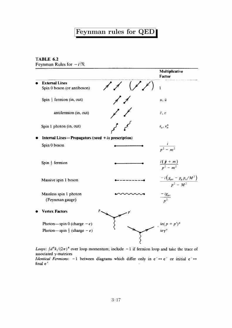
Feynman rules for QED

!

3–17