arX

iv:a

stro

-ph/

0603

092v

1 3

Mar

200

6

Gauge Freedom in Orbital Mechanics.

Michael EfroimskyUS Naval Observatory, Washington DC 20392 USA

January 14, 2014

Abstract

Both orbital and attitude dynamics employ the method of variation of parameters. Ina non-perturbed setting, the coordinates (or the Euler angles) get expressed as functionsof the time and six adjustable constants called elements. Under disturbance, each suchexpression becomes ansatz, the “constants” being endowed with time dependence. Theperturbed velocity (linear or angular) consists of a partial time derivative and a convectiveterm containing time derivatives of the “constants.” It can be shown that this construc-tion leaves one with a freedom to impose three arbitrary conditions upon the “constants”and/or their derivatives. Out of convenience, the Lagrange constraint is often imposed.It nullifies the convective term and thereby guarantees that under perturbation the func-tional dependence of the velocity upon the time and “constants” stays the same as in theundisturbed case. “Constants” obeying this condition are called osculating elements.

The “constants” chosen to be canonical, are called Delaunay elements, in the orbitalcase, or Andoyer elements, in the spin case. (As some of the Andoyer elements are time-dependent even in the free-spin case, the role of “constants” is played by these elements’initial values.) The Andoyer and Delaunay sets of elements share a feature not readilyapparent: in certain cases the standard equations render these elements non-osculating.

In orbital mechanics, elements calculated via the standard planetary equations comeout non-osculating when perturbations depend on velocities. To keep elements osculatingunder such perturbations, the equations must be amended with extra terms that are notparts of the disturbing function (Efroimsky and Goldreich 2003, 2004). For the Kepler el-ements, this merely complicates the equations. In the case of Delaunay parameterisation,these extra terms not only complicate the equations, but also destroy their canonicity.So under velocity-dependent disturbances, osculation and canonicity are incompatible.

Similarly, in spin dynamics the Andoyer elements come out non-osculating underangular-velocity-dependent perturbation (a switch to a noninertial frame being one suchcase). Amendment of the dynamical equations only with extra terms in the Hamiltonianmakes the equations render nonosculating Andoyer elements. To make them osculating,more terms must enter the equations (and the equations will no longer be canonical).

It is often convenient to deliberately deviate from osculation by substituting the La-grange constraint with an arbitrary condition that gives birth to a family of nonosculat-ing elements. The freedom in choosing this condition is analogous to the gauge freedom.Calculations in nonosculating variables are mathematically valid and sometimes highlyadvantageous, but their physical interpretation is nontrivial. For example, nonosculat-ing orbital elements parameterise instantaneous conics not tangent to the orbit, so thenonosculating inclination will be different from the real inclination of the physical orbit.

We present examples of situations in which ignoring of the gauge freedom (and of theunwanted loss of osculation) leads to oversights.

1

1 Introduction

1.1 Historical Prelude

The orbital dynamics is based on the variation-of-parameters method, invention whereof isattributed to Euler (1748, 1753) and Lagrange (1778, 1783, 1808, 1809, 1810). Though bothgreatly contributed to this approach, its initial sketch was offered circa 1687 by Newton in hisunpublished Portsmouth Papers. Very succinctly, Newton brought up this issue also in Cor. 3and 4 of Prop. 17 in the first book of his Principia.

Geometrically, the part and parcel of this method is representation of an orbit as a set ofpoints, each of which is contributed by a member of some chosen family of curves C(κ), whereκ stands for a set of constants that number a particular curve within the family. (For example,a set of three constants κ = a, b, c defines one particular hyperbola y = ax2 + bx + cout of many). This situation is depicted on Fig.1. Point A of the orbit coincides with somepoint λ1 on a curve C(κ1). Point B of the orbit coincides with point λ2 on some other curveC(κ2) of the same family, etc. This way, orbital motion from A to B becomes a superpositionof motion along Cκ from λ1 to λ2 and a gradual distortion of the curve Cκ from the shapeC(κ1) to the shape C(κ2). In a loose language, the motion along the orbit consists of stepsalong an instantaneous curve C(κ) which itself is evolving while those steps are being made.

Fig.1. Each point of the orbit is contributed by a member of some family ofcurves C(κ) of a certain type, κ standing for a set of constants that numbera particular curve within the family. Motion from A to B is, first, due to themotion along the curve C(κ) from λ1 to λ2 and, second, due to the factthat during this motion the curve itself was evolving from C(κ1) to C(κ2) .

2

Normally, the family of curves Cκ is chosen to be that of ellipses or that of hyperbolae, κ beingsix orbital elements, and λ being the time. However, if we disembody this idea of its customaryimplementation, we shall see that it is of a far more general nature and contains three aspects:

1. A trajectory may be assembled of points contributed by a family of curves of an essen-tially arbitrary type, not just conics.

2. It is not necessary to choose the family of curves tangent to the orbit. As we shall seebelow, it is often beneficial to choose them nontangent. We shall also see examples when inorbital calculations this loss of tangentiality (loss of osculation) takes place and goes unnoticed.

3. The approach is general and can be applied, for example, to Euler’s angles. A disturbedrotation can be thought of as a series of steps (small turns) along different Eulerian cones. AnEulerian cone is an orbit (on the Euler angles’ manifold) corresponding to an unperturbed spinstate. Just as a transition from one instantaneous Keplerian conic to another is caused by dis-turbing forces, so a transition from one instantaneous Eulerian cone to another is dictated byexternal torques or other perturbations. Thus, in the attitude mechanics, the Eulerian conesplay the same role as the Keplerian conics do in the orbital dynamics. Most importantly, aperturbed rotation may be “assembled” of the Eulerian cones in an osculating or in a nonoscu-lating manner. An unwanted loss of osculation in attitude mechanics happens in the sameway as in the theory of orbits, but is much harder to notice. On the other hand, a deliberatechoice of nonosculating rotational elements in attitude mechanics may sometimes be beneficial.

From the viewpoint of calculus, the concept of variation of parameters looks as follows. Wehave a system of differential equations to solve (“system in question”) and a system of differ-ential equations (“fiducial system”) whose solution is known and contains arbitrary constants.We then use the known solution to the fiducial system as an ansatz for solving the system inquestion. The constants entering this ansatz are endowed with time dependence of their own,and the subsequent substitution of this known solution into the system in question yields equa-tions for the “constants.” The number of “constants” often exceeds that of equations in thesystem to solve. In this case we impose, by hand, arbitrary constraints upon the “constants.”For example, in the case of a reduced N -body problem, we begin with 3(N − 1) unconstrainedsecond-order equations for 3(N − 1) Cartesian coordinates. After a change of variables fromthe Cartesian coordinates to the orbital parameters, we end up with 3(N − 1) differentialequations for the 6(N − 1) orbital variables. Evidently, 3(N − 1) constraints are necessary.1

To this end, the so-called Lagrange constraint (the condition of the instantaneous conics being

1 In a fixed Cartesian frame, any solution to the unperturbed reduced 2-body problem can be written as

xj = fj(t , C1 , . . . , C6) , j = 1 , 2 , 3 ,

xj = gj(t , C1 , . . . , C6) , gj ≡(

∂fj

∂t

)

C

the adjustable constants C standing for orbital elements. Under disturbance, the solution is sought as

xj = fj(t , C1(t) , . . . , C6(t) ) , j = 1 , 2 , 3 ,

xj = gj(t , C1(t) , . . . , C6(t) ) + Φj(t , C1(t) , . . . , C6(t) ) , gj ≡(

∂fj

∂t

)

C

, Φj ≡∑

r

∂fj

∂Cr

Cr .

Insertion of xj = fj(t, C) into the perturbed gravity law yields three scalar equations for six functions Cr(t).

This necessitates imposition of three conditions upon Cr and Cr . Under the simplest choice Φj = 0 , j = 1, 2, 3,the perturbed physical velocity xj(t, C) has the same functional form as the unperturbed gj(t, C) . Therefore,the instantaneous conics become tangent to the orbit (and the orbital elements Cr(t) are called osculating).

3

tangent to the physical orbit) is introduced almost by default, because it is regarded natural.Two things should be mentioned in this regard:

First, what seems natural is not always optimal. The freedom of choice of the supplementarycondition (the gauge freedom) gives birth to an internal symmetry (the gauge symmetry) ofthe problem. Most importantly, it can be exploited for simplifying the equations of motion forthe “constants.” On this issue we shall dwell in the current paper.

Second, the entire scheme may, in principle, be reversed and used to solve systems of differ-ential equations with constraints. Suppose we have N + M variables Cj(t) obeying a systemof N differential equations of the second order and M constraints expressed with first-orderdifferential equations or with algebraic expressions. One possible approach to solving this sys-tem will be to assume that the variables Cj come about as constants emerging in a solution tosome fiducial system of differential equations. Then our N second-order differential equationsfor Cj(t) will be interpreted as a result of substitution of such an ansatz into the fiducialsystem with some perturbation, while our M constraints will be interpreted as weeding out ofthe redundant degrees of freedom. Unfortunately, this subject is out of the scope of our paper,and it will be developed somewhere else.

1.2 The simplest example of gauge freedom.

Variation of constants first emerged in the nonlinear context of celestial mechanics and laterbecame a universal tool. We begin with a simple example offered in Newman & Efroimsky(2003)

A harmonic oscillator disturbed by a force ∆F (t) gives birth to the initial-condition problem

x + x = ∆F (t) , with x(0) and x(0) known , (1)

whose solution may be sought using ansatz

x = C1(t) sin t + C2(t) cos t . (2)

This will lead us to

x =[

C1(t) sin t + C2(t) cos t]

+ C1(t) cos t − C2(t) sin t . (3)

It is common, at this point, to put the sum[

C1(t) sin t + C2(t) cos t]

equal to zero, in order toremove the ambiguity stemming from the fact that we have only one equation for two variables.Imposition of this constraint is convenient but not obligatory. A more general way of fixingthe ambiguity may be expressed as

C1(t) sin t + C2(t) cos t = φ(t) , (4)

φ(t) being an arbitrary function of time. This entails:

x = φ + C1(t) cos t − C2(t) sin t − C1(t) sin t − C2(t) cos t , (5)

summation whereof with (2) gives:

x + x = φ + C1(t) cos t − C2(t) sin t . (6)

4

Substitution thereof into (1) yields the dynamical equation re-written in terms of the “con-stants” C1 , C2 . This equation, together with identity (4), will constitute the following system:

φ + C1(t) cos t − C2(t) sin t = ∆F (t) ,

(7)

C1(t) sin t + C2(t) cos t = φ(t) ,

This leads to

C1 = ∆F cos t − d

dt(φ cos t)

(8)

C2 = −∆F sin t +d

dt(φ sin t) ,

the function φ(t) still remaining arbitrary.2 Integration of (8) entails:

C1 =∫ t

∆F cos t′ dt′ − φ cos t + a1

(9)

C2 = −∫ t

∆F sin t′ dt′ + φ sin t + a2 .

Substitution of (9) into (2) leads to complete cancellation of the φ terms:

x = C1 sin t + C2 cos t = − cos t∫ t

∆F sin t′ dt′ + sin t∫ t

∆F cos t′ dt′ + a1 sin t + a2 cos t (10)

Naturally, the physical trajectory x(t) remains invariant under the choice of gauge functionφ(t) , even though the mathematical description (9) of this motion in terms of the parametersC is gauge dependent. It is, however, crucial that a numerical solution of the system (8) willcome out φ-dependent, because the numerical error will be sensitive to the choice of φ(t). Thisissue is now being studied by P. Gurfil and I. Klein, and the results are to be published soon.(Gurfil & Klein 2006)

It remains to notice that (8) is a simple analogue to the Lagrange-type system of planetaryequations, system that, too, admits gauge freedom. (See subsection 2.2 below.)

1.3 Gauge freedom under a variation of the Lagrangian

The above example permits an evident extension. (Efroimsky 2002a,b.) Suppose some me-chanical system obeys the equation

r = F ( t , r , r ) , (11)

whose solution is known and has a functional form

r = f ( t , C1 , . . . , C6 ) , (12)

2 Function φ(t) can afford being arbitrary, no matter what the initial conditions are to be. Indeed, for fixedx(0) and x(0), the system C2(0) = x(0) , φ(0) + C1(0) = x(0) solves for C1(0) and C2(0) for an arbitrarychoice of φ(0).

5

Cj being adjustable constants to vary only under disturbance.When a perturbation ∆F gets switched on, the system becomes:

r = F ( t , r , r ) + ∆F ( t , r , r ) , (13)

and its solution will be sought in the form of

r = f ( t , C1(t) , . . . , C6(t) ) . (14)

Evidently,

r =∂f

∂t+ Φ , Φ ≡

6∑

j=1

∂f

∂CjCj . (15)

In defiance of what the textbooks advise, we do not put Φ nil. Instead, we proceed further to

r =∂2f

∂t2+

6∑

j=1

∂2f

∂t ∂CjCj + Φ , (16)

dot standing for a full time derivative. If we now insert the latter into the perturbed equationof motion (13) and if we recall that, according to (11),3 ∂2f/∂t2 = F , then we shall obtainthe equation of motion for the new variables Cj(t) :

6∑

j=1

∂2f

∂t ∂CjCj + Φ = ∆F (17)

where

Φ ≡6∑

j=1

∂f

∂Cj

Cj (18)

so far is merely an identity. It will become a constraint after we choose a particular functional

form Φ (t ; C1 , . . . , C6) for the gauge function Φ , i.e., if we choose that the sum∑ ∂f

∂CjCj

be equal to some arbitrarily fixed function Φ(t ; C1 , . . . , C6) of the time and of the variable“constants.” This arbitrariness exactly parallels the gauge invariance in electrodynamics: onthe one hand, the choice of the functional form of Φ(t ; C1 , . . . , C6) will never4 influence theeventual solution for the physical variable r ; on the other hand, though, a qualified choicemay considerably simplify the process of finding the solution. To illustrate this, let us denoteby g(t , C1 , . . . , C6) the functional dependence of the unperturbed velocity on the time andadjustable constants:

g(t , C1 , . . . , C6) ≡ ∂

∂tf (t , C1 , . . . , C6) , (19)

3 We remind that in (11) there was no difference between a partial and a full time derivative, because atthat point the integration “constants” Ci were indeed constant. Later, they acquired time dependence, andtherefore the full time derivative implied in (15 - 16) became different from the partial one implied in (11).

4 Our usage of words “arbitrary” and “never” should be limited to the situations where the chosen gauge(21) does not contradict the equations of motion (20). This restriction, too, parallels a similar one present infield theories. Below we shall encounter a situation where this restriction becomes crucial.

6

and rewrite the above system as

∑

j

∂g

∂CjCj = − Φ + ∆F (20)

∑

j

∂f

∂CjCj = Φ . (21)

If we now dot-multiply the first equation with ∂f/∂Ci and the second one with ∂g/∂Ci ,and then take the difference of the outcomes, we shall arrive at

∑

j

[ Cn Cj ] Cj =(

∆F − Φ)

· ∂f

∂Cn− Φ · ∂g

∂Cn, (22)

the Lagrange brackets being defined in a gauge-invariant (i.e., Φ-independent) fashion.5 Ifwe agree that Φ is a function of both the time and the parameters Cn , but not of theirderivatives,6 then the right-hand side of (22) will implicitly contain the first time derivativesof Cn . It will then be reasonable to move these to the left-hand side. Hence, (22) will bereshaped into

∑

j

(

[Cn Cj] +∂f

∂Cn

· ∂Φ

∂Cj

)

dCj

dt=

∂f

∂Cn

· ∆F − ∂f

∂Cn

· ∂Φ

∂t− ∂g

∂Cn

· Φ . (23)

This is the general form of the gauge-invariant perturbation equations, that follows fromthe variation-of-parameters method applied to problem (13), for an arbitrary perturbationF (r, r, t) and under the simplifying assumption that the arbitrary gauge function Φ ischosen to depend on the time and the parameters Cn , but not on their derivatives.7 As-sume that our problem (13) is not simply mathematical but is an equation of motion for some

5 The Lagrange-bracket matrix is defined in a gauge-invariant way:

∑

j

[ Cn Cj ] ≡ ∂f

∂Cn

· ∂g

∂Cj

− ∂~g

∂Cn

· ∂f

∂Cj

.

and so is its inverse, the matrix composed of the Poisson brackets

Cn Cj ≡ ∂Cn

∂f· ∂Cj

∂g− ∂Cn

∂g· ∂Cj

∂f.

Evidently, (22) yields

Cn =∑

j

Cn Cj [

∂f

∂Cj

·(

∆F − Φ)

− Φ · ∂g

∂Cj

]

.

6 The necessity to fix a functional form of Φ( t ; C1 , . . . , C6 ) , i.e., to impose three arbitrary conditionsupon the “constants” Cj , evidently follows from the fact that, on the one hand, in the ansatz (14) we have sixvariables Cn(t) and, on the other hand, the number of scalar equations of motion (i.e., Cartesian projectionsof the perturbed vector equation (13) ) is only three. This necessity will become even more mathematicallytransparent after we cast the perturbed equation (13) into the normal form of Cauchy. (See Appendix.)

7 We may also impart the gauge function with dependence upon the parameters’ time derivatives of allorders. This will yield higher-than-first-order derivatives in equation (23). In order to close this system, onewill then have to impose additional initial conditions, beyond those on r and r .

7

physical setting, so that F is a physical force corresponding to some undisturbed LagrangianLo , and ∆F is a force perturbation generated by a Lagrangian variation ∆L . If, for exam-ple, we begin with Lo(r , r , t) = r 2/2 − U(r , t) , momentum p = r , and HamiltonianHo(r , p , t) = p2/2 + U(r , t) , then their disturbed counterparts will read:

L(r , r , t) =r 2

2− U(r) + ∆L(r, r, t) , (24)

p = r +∂∆L∂r

, (25)

H = p r − L =p 2

2+ U + ∆H , (26)

∆H ≡ − ∆L − 1

2

(

∂ ∆L∂r

)2

. (27)

The Euler-Lagrange equations written for the perturbed Lagrangian (24) are:

r = − ∂U

∂r+ ∆F , (28)

where the disturbing force is given by

∆F ≡ ∂ ∆L∂r

− d

dt

(

∂ ∆L∂r

)

. (29)

Its substitution in (23) yields the generic form of the equations in terms of the Lagrangiandisturbance (Efroimsky & Goldreich 2004):

∑

j

(

[Cn Cj] +∂f

∂Cn

· ∂

∂Cj

(

∂ ∆L∂r

+ Φ

) )

dCj

dt=

(30)

∂

∂Cn

∆L +1

2

(

∂ ∆L∂r

)2

−(

∂g

∂Cn

+∂f

∂Cn

∂

∂t+

∂ ∆L∂r

∂

∂Cn

)

·(

Φ +∂ ∆L∂r

)

.

This equation not only reveals the convenience of the special gauge

Φ = − ∂ ∆L∂r

, (31)

(which reduces to Φ = 0 in the case of velocity-independent perturbations), but also explicitlydemonstrates how the Hamiltonian variation comes into play: it is easy to notice that, accordingto (27), the sum in square brackets on the right-hand side of (30) is equal to − ∆H , so theabove equation takes the form

∑

j [Cn Cj ] Cj = − ∂∆H/∂Cn . All in all, it becomesclear that the trivial gauge, Φ = 0 , leads to the maximal simplification of the variation-of-parameters equations expressed through the disturbing force: it follows from (22) that

∑

j

[ Cn Cj ] Cj = ∆F · ∂f

∂Cn, provided we have chosen Φ = 0 . (32)

8

However, the choice of the special gauge (31) entails the maximal simplification of the variation-of-parameters equations when they are formulated via a variation of the Hamiltonian:

∑

j

[Cn Cj ]dCj

dt= − ∂∆H

∂Cn, provided we have chosen Φ = − ∂ ∆L

∂r. (33)

It remains to spell out the already obvious fact that, in case the unperturbed force F isgiven by the Newton gravity law (i.e., when the undisturbed setting is the reduced two-bodyproblem), then the variable “constants” Cn are merely the orbital elements parameterising asequence of instantaneous conics out of which we “assemble” the perturbed trajectory through(14). When the conics’ parameterisation is chosen to be via the Kepler or the Delaunay vari-ables, then (30) yields the gauge-invariant version of the Lagrange-type or the Delaunay-typeplanetary equations, accordingly. Similarly, (22) implements the gauge-invariant generalisationof the planetary equations in the Euler-Gauss form.

From (22) we see that the Euler-Gauss-type planetary equations will always assume theirsimplest form (32) under the gauge choice Φ = 0 . In astronomy this choice is called“the Lagrange constraint.” It makes the orbital elements osculating, i.e., guarantees that theinstantaneous conics, parameterised by these elements, are tangent to the perturbed orbit.

From (33) one can easily notice that the Lagrange- and Delaunay-type planetary equationssimplify maximally under the condition (31). This condition coincides with the Lagrangeconstraint Φ = 0 when the perturbation depends only upon positions (not upon velocities ormomenta). Otherwise, condition (31) deviates from that of Lagrange, and the orbital elementsrendered by equation (33) are no longer osculating (so that the corresponding instantaneousconics are no longer tangent to the physical trajectory).

Of an even greater importance will be the following observation. If we have a velocity-dependent perturbing force, we can always find the appropriate Lagrangian variation and,therefrom, the corresponding variation of the Hamiltonian. If now we simply add the negativeof this Hamiltonian variation to the disturbing function, then the resulting equations (33) willrender not the osculating elements but orbital elements of a different type, ones satisfyingthe non-Lagrange constraint (31). Since the instantaneous conics, parameterised by such non-osculating elements, will not be tangent to the orbit, then physical interpretation of suchelements may be nontrivial. Besides, they will return a velocity different from the physicalone.8 This pitfall is well camouflaged and is easy to fall in.

These and other celestial-mechanics applications of the gauge freedom will be consideredin detail in section 2 below.

1.4 Canonicity versus osculation

One more relevant development will come from the theory of canonical perturbations. Supposethat in the absence of disturbances we start out with a system

q =∂H(o)

∂p, p = − ∂H(o)

∂q. (34)

q and p being the Cartesian or polar coordinates and their conjugated momenta, in theorbital case, or the Euler angles and their momenta, in the rotation case. Then we switch, via

8 We mean that substitution of the values of these elements in g(t ; C1(t) , . . . , C6(t)) will not give theright velocity. The correct physical velocity will be given by r = g + Φ .

9

a canonical transformation

q = f(Q , P , t) , p = χ(Q , P , t) (35)

to

Q =∂H∗

∂P= 0 , P = − ∂H∗

∂Q= 0 , H∗ = 0 , (36)

where Q and P denote the set of Delaunay elements, in the orbital case, or the initial valuesof the Andoyer variables, in the case of rigid-body rotation.

This scheme relies on the fact that, for an unperturbed motion (i.e., for an unperturbedKeplerian conic, in an orbital case; or for an undisturbed Eulerian cone, in the spin case) asix-constant parameterisation may be chosen so that:

1. the parameters are constants and, at the same time, are canonical variables Q , P with a zero Hamiltonian H∗(Q, P ) = 0 ;

2. for constant Q and P , the transformation equations (35) are mathematically equiva-lent to the dynamical equations (34).

Under perturbation, the “constants” Q, P begin to evolve so that, after their substitution into

q = f (Q(t) , P (t) , t ) , p = χ( Q(t) , P (t) , t ) , (37)

(f, χ being the same functions as in (35) ), the resulting motion obeys the disturbed equations

q =∂(

H(o) + ∆H)

∂p, p = −

∂(

H(o) + ∆H)

∂q. (38)

We also want our “constants” Q and P to remain canonical and to obey

Q =∂ (H∗ + ∆H∗)

∂P, P = − ∂ (H∗ + ∆H∗)

∂Q(39)

where

H∗ = 0 and ∆H∗ (Q , P t) = ∆H ( q(Q, P, t) , p(Q, P, t) , t ) . (40)

Above all, we wish the perturbed “constants” C = Q, P (the Delaunay elements, in theorbital case; or the initial values of the Andoyer elements, in the spin case) to osculate. Thismeans that we want the perturbed velocity to be expressed by the same function of Cj(t) andt as the unperturbed velocity. Let us check when this is possible. The perturbed velocity is

q = g + Φ (41)

where

g(C(t), t) ≡ ∂q(C(t), t)

∂t(42)

10

is the functional expression for the unperturbed velocity, while

Φ(C(t), t) ≡6∑

j=1

∂q(C(t), t)

∂Cj

Cj(t) (43)

is the convective term. Since we chose the “constants” Cj to make canonical pairs (Q, P )obeying (39 - 40), then insertion of (39) into (43) will result in

Φ =3∑

n=1

∂q

∂QnQn(t) +

3∑

n=1

∂q

∂PnPn(t) =

∂∆H(q, p)

∂p. (44)

So canonicity is incompatible with osculation when ∆H depends on p. Our desire to keepthe perturbed equations (39) canonical makes the orbital elements Q , P nonosculating ina particular manner prescribed by (44). This breaking of gauge invariance reveals that thecanonical description is marked with “gauge stiffness” (term suggested by Peter Goldreich).

We see that, under a momentum-dependent perturbation, we still can use the ansatz (37) forcalculation of the coordinates and momenta, but can no longer use q = ∂q/∂t for calculatingthe velocities. Instead, we must use q = ∂q/∂t + ∂∆H/∂p , and the elements Cj will nolonger be osculating. In the case of orbital motion (when Cj are the nonosculating Delaunayelements), this will mean that the instantaneous ellipses or hyperbolae parameterised by theseelements will not be tangent to the orbit. (Efroimsky & Goldreich 2003.) In the case of spin,the situation will be similar, except that, instead of an instantaneous Keplerian conic, onewill be dealing with an instantaneous Eulerian cone – a set of trajectories on the Euler-anglesmanifold, each of which corresponds to some non-perturbed spin state. (Efroimsky 2004.)

The main conclusion to be derived from this example is the following: whenever we en-counter a disturbance that depends not only upon positions but also upon velocities or mo-menta, implementation of the afore described canonical-perturbation method necessarily yieldsequations that render nonosculating canonical elements. It is possible to keep the elements os-culating, but only at the cost of sacrificing canonicity. For example, under velocity-dependentorbital perturbations (like inertial forces, or atmospheric drag, or relativistic correction) theequations for osculating Delaunay elements will no longer be Hamiltonian (Efroimsky 2002a,b).

Above in this subsection we discussed the disturbed velocity q . How about the disturbedmomentum? For sufficiently simple unperturbed Hamiltonians, it can be written down veryeasily. For example, for H = Ho + ∆H = p2/2m + U(q) + ∆H we get:

p = q +∂∆L∂q

= g + Φ +∂∆L∂q

= g +

(

Φ − ∂∆H∂q

)

= g . (45)

In this case, the perturbed momentum p coincides with the unperturbed one, g. In applicationto the orbital motion, this means that contact elements (i.e., the nonosculating orbital elementsobeying (31) ), when substituted in g(t ; C1 , . . . , C6), furnish not the correct perturbed velocitybut the correct perturbed momentum, i.e., they osculate the orbit in phase space. Existenceof such elements was pointed out long ago by Goldreich (1965) and Brumberg et al (1971).

11

2 Gauge freedom in the theory of orbits.

2.1 Geometrical meaning of the arbitrary gauge function Φ

As explained above, the content of subsection 1.3 becomes merely a formulation of the Lagrangetheory of orbits, provided F stands for the Newton gravity force, so that the undisturbedsetting is the two-body problem. Then (22) expresses the gauge-invariant (i.e., taken withan arbitrary gauge Φ(t ; C1 , . . . , C6) ) planetary equations in the Euler-Gauss form. Theseequations render orbital elements that are, generally, not osculating. Equation (32) stands forthe customary Euler-Gauss-type system for osculating (i.e., obeying Φ = 0 ) orbital elements.

Similarly, equation (30) stands for the gauge-invariant Lagrange-type or Delaunay-type(dependent upon whether Ci stand for the Kepler or Delaunay variables) equations. Suchequations yield elements, which, generally, are not osculating. In those equations, one couldfix the gauge by putting Φ = 0 , thus making the resulting orbital elements osculating. How-ever, this would be advantageous only in the case of velocity-independent ∆L . Otherwise, amaximal simplification is achieved through a deliberate refusal from osculation: by choosingthe gauge as (31) one ends up with simple equations (33). Thus, gauge (31) simplifies theplanetary equations. (See equations (46 - 57) below.) Besides, in the case when the Delau-nay parameterisation is employed, this gauge makes the equations for the Delaunay variablescanonical for reasons explained above in subsection 1.4.

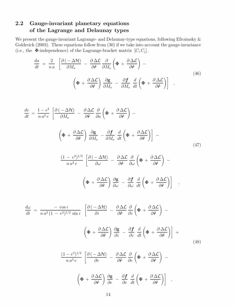
The geometrical meaning of the convective term Φ becomes evident if we recall that aperturbed orbit is assembled of points, each of which is donated by one representative of asequence of conics, as on Fig.2 and Fig.3 where the “walk” over the instantaneous conics maybe undertaken either in a non-osculating manner or in the osculating manner. The physicalvelocity r is always tangent to the perturbed orbit, while the unperturbed Keplerian velocityg ≡ ∂f/∂t is tangent to the instantaneous conic. Their difference is the convective term Φ.So if we use non-osculating orbital elements, then insertion of their values in f (t ; C1 , . . . , C6)will yield a correct position of the body. However, their insertion in g(t ; C1 , . . . , C6) willNOT give the right velocity. To get the correct velocity, one will have to add Φ . (See Appendixfor a more formal mathematical treatment in the normal form of Cauchy.)

When using non-osculating orbital elements, we must always be careful about their physicalinterpretation. On Fig. 2, the instantaneous conics are not supposed to be tangent to theorbit, nor are they supposed to be even coplanar thereto. (They may be even perpendicularto the orbit! – why not?) This means that, for example, the non-osculating element i mayconsiderably differ from the real, physical inclination of the orbit.

We would add that the arbitrariness of choice of the function Φ(t , C1(t) , . . . , C6(t)) hadbeen long known but never used in astronomy until a recent effort undertaken by several authors(Efroimsky 2002a,b ; Newman & Efroimsky 2003; Slabinski 2003; Efroimsky & Goldreich2003, 2004; Gurfil 2004; Efroimsky 2005c) Substitution of the Lagrange constraint Φ = 0with alternative choices does not influence the physical motion, but alters its mathematicaldescription (i.e., renders different values of the orbital parameters Ci(t)). Such invariance of aphysical picture under a change of parameterisation goes under the name of gauge freedom. Itis a part and parcel of electrodynamics and other field theories. In mathematics, it is describedin terms of fiber bundles. A clever choice of gauge often simplifies solution of the equationsof motion. On the other hand, the gauge invariance may have implications upon numericalprocedures. We mean the so-called ”gauge drift,” i.e., unwanted displacement in the gaugefunction Φ, caused by accumulation of numerical errors in the constants.

12

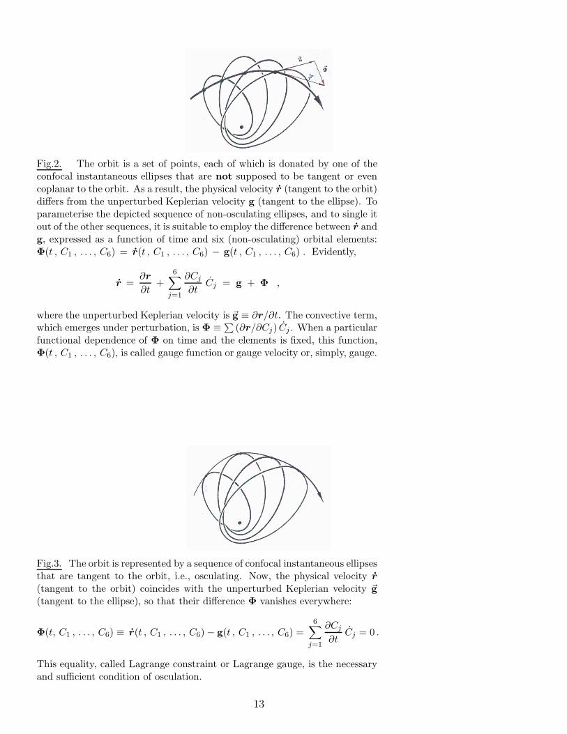
Fig.2. The orbit is a set of points, each of which is donated by one of theconfocal instantaneous ellipses that are not supposed to be tangent or evencoplanar to the orbit. As a result, the physical velocity r (tangent to the orbit)differs from the unperturbed Keplerian velocity g (tangent to the ellipse). Toparameterise the depicted sequence of non-osculating ellipses, and to single itout of the other sequences, it is suitable to employ the difference between r andg, expressed as a function of time and six (non-osculating) orbital elements:Φ(t , C1 , . . . , C6) = r(t , C1 , . . . , C6) − g(t , C1 , . . . , C6) . Evidently,

r =∂r

∂t+

6∑

j=1

∂Cj

∂tCj = g + Φ ,

where the unperturbed Keplerian velocity is ~g ≡ ∂r/∂t. The convective term,which emerges under perturbation, is Φ ≡∑

(∂r/∂Cj) Cj . When a particularfunctional dependence of Φ on time and the elements is fixed, this function,Φ(t , C1 , . . . , C6), is called gauge function or gauge velocity or, simply, gauge.

Fig.3. The orbit is represented by a sequence of confocal instantaneous ellipsesthat are tangent to the orbit, i.e., osculating. Now, the physical velocity r

(tangent to the orbit) coincides with the unperturbed Keplerian velocity ~g(tangent to the ellipse), so that their difference Φ vanishes everywhere:

Φ(t, C1 , . . . , C6) ≡ r(t , C1 , . . . , C6) − g(t , C1 , . . . , C6) =6∑

j=1

∂Cj

∂tCj = 0 .

This equality, called Lagrange constraint or Lagrange gauge, is the necessaryand sufficient condition of osculation.

13

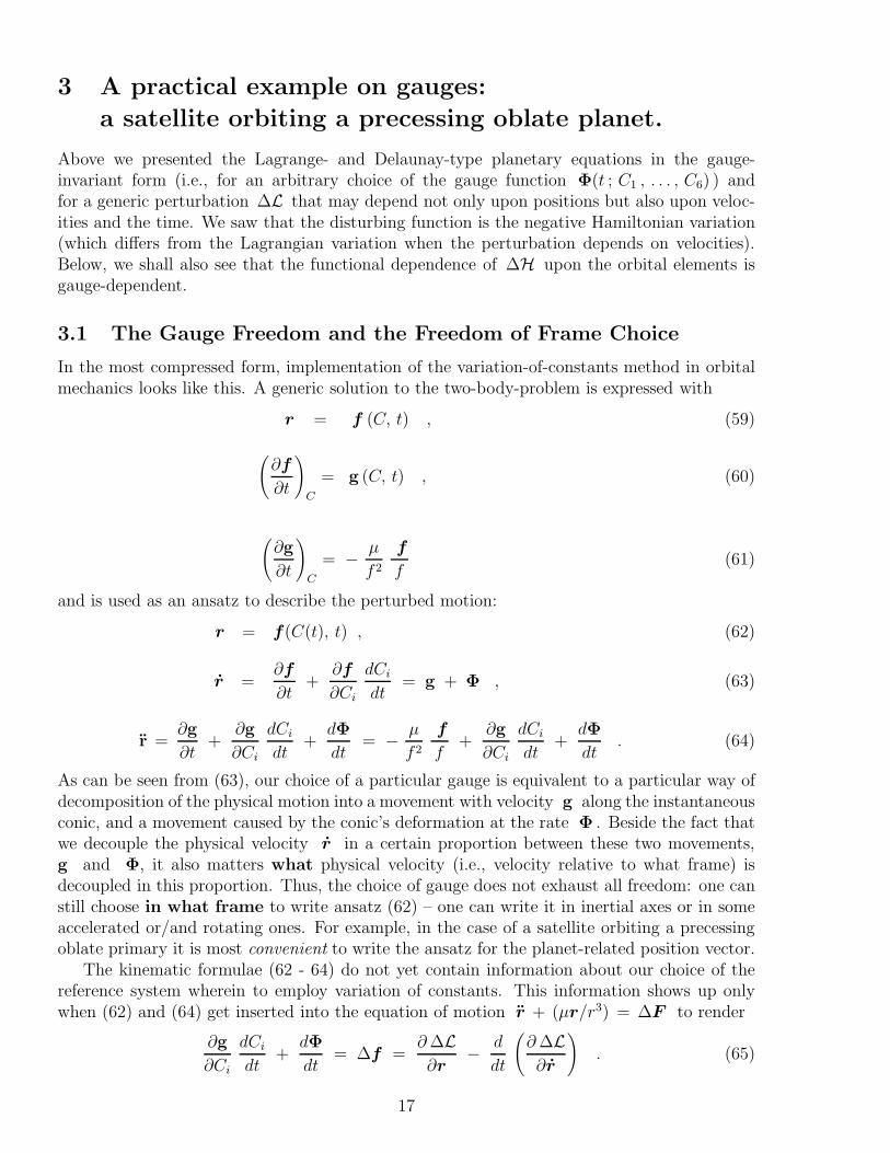
2.2 Gauge-invariant planetary equations

of the Lagrange and Delaunay types

We present the gauge-invariant Lagrange- and Delaunay-type equations, following Efroimsky &Goldreich (2003). These equations follow from (30) if we take into account the gauge-invariance(i.e., the Φ-independence) of the Lagrange-bracket matrix [Ci Cj] .

da

dt=

2

n a

[

∂ (−∆H)

∂Mo− ∂ ∆L

∂r

∂

∂Mo

(

Φ +∂ ∆L∂r

)

−

(46)(

Φ +∂ ∆L∂r

)

∂g

∂Mo

− ∂f

∂Mo

d

dt

(

Φ +∂ ∆L∂r

)]

,

de

dt=

1 − e2

n a2 e

[

∂ (−∆H)

∂Mo− ∂ ∆L

∂r

∂

∂a

(

Φ +∂ ∆L∂r

)

−

(

Φ +∂ ∆L∂r

)

∂g

∂Mo− ∂f

∂Mo

d

dt

(

Φ +∂ ∆L∂r

)]

−

(47)

(1 − e2)1/2

n a2 e

[

∂ (−∆H)

∂ω− ∂ ∆L

∂r

∂

∂ω

(

Φ +∂ ∆L∂r

)

−

(

Φ +∂ ∆L∂r

)

∂g

∂ω− ∂f

∂ω

d

dt

(

Φ +∂ ∆L∂r

)]

,

dω

dt=

− cos i

n a2 (1 − e2)1/2 sin i

[

∂ (−∆H)

∂i− ∂ ∆L

∂r

∂

∂i

(

Φ +∂ ∆L∂r

)

−

(

Φ +∂ ∆L∂r

)

∂g

∂i− ∂f

∂i

d

dt

(

Φ +∂ ∆L∂r

)]

+

(48)

(1 − e2)1/2

n a2 e

[

∂ (−∆H)

∂e− ∂ ∆L

∂r

∂

∂e

(

Φ +∂ ∆L∂r

)

−

(

Φ +∂ ∆L∂r

)

∂g

∂e− ∂f

∂e

d

dt

(

Φ +∂ ∆L∂r

)]

,

14

di

dt=

cos i

n a2 (1 − e2)1/2 sin i

[

∂ (−∆H)

∂ω− ∂ ∆L

∂r

∂

∂ω

(

Φ +∂ ∆L∂r

)

−

(

Φ +∂ ∆L∂r

)

∂g

∂ω− ∂f

∂ω

d

dt

(

Φ +∂ ∆L∂r

)]

−

(49)

1

n a2 (1 − e2)1/2 sin i

[

∂ (−∆H)

∂Ω− ∂ ∆L

∂r

∂

∂Ω

(

Φ +∂ ∆L∂r

)

−

(

Φ +∂ ∆L∂r

)

∂g

∂Ω− ∂f

∂Ω

d

dt

(

Φ +∂ ∆L∂r

)]

,

dΩ

dt=

1

n a2 (1 − e2)1/2 sin i

[

∂ (−∆H)

∂i− ∂ ∆L

∂r

∂

∂i

(

Φ +∂ ∆L∂r

)

−

(50)(

Φ +∂ ∆L∂r

)

∂g

∂i− ∂f

∂i

d

dt

(

Φ +∂ ∆L∂r

)]

,

dMo

dt= − 1 − e2

n a2 e

[

∂ (−∆H)

∂e− ∂ ∆L

∂r

∂

∂e

(

Φ +∂ ∆L∂r

)

−

(

Φ +∂ ∆L∂r

)

∂g

∂e− ∂f

∂e

d

dt

(

Φ +∂ ∆L∂r

)]

−

(51)

2

n a

[

∂ (−∆H)

∂a− ∂ ∆L

∂r

∂

∂a

(

Φ +∂ ∆L∂r

)

−

(

Φ +∂ ∆L∂r

)

∂g

∂a− ∂f

∂a

d

dt

(

Φ +∂ ∆L∂r

)]

.

15

Similarly, the gauge-invariant Delaunay-type system can be written down as:

dL

dt=

∂ (−∆H)

∂Mo− ∂ ∆L

∂r

∂

∂Mo

(

Φ +∂ ∆L∂r

)

−(

Φ +∂ ∆L∂r

)

∂g

∂Mo− ∂r

∂Mo

d

dt

(

Φ +∂ ∆L∂r

)

, (52)

dMo

dt= − ∂ (−∆H)

∂L+

∂ ∆L∂r

∂

∂L

(

Φ +∂ ∆L∂r

)

+

(

~Φ +∂ ∆L∂r

)

∂g

∂L+

∂r

∂L

d

dt

(

Φ +∂ ∆L∂r

)

, (53)

dG

dt=

∂ (−∆H)

∂ω− ∂ ∆L

∂r

∂

∂ω

(

Φ +∂ ∆L∂r

)

−(

Φ +∂ ∆L∂r

)

∂g

∂ω− ∂r

∂ω

d

dt

(

Φ +∂ ∆L∂r

)

, (54)

dω

dt= − ∂ (−∆H)

∂G+

∂ ∆L∂r

∂

∂G

(

Φ +∂ ∆L∂r

)

+

(

Φ +∂ ∆L∂r

)

∂g

∂G+

∂r

∂G

d

dt

(

Φ +∂ ∆L∂r

)

, (55)

dH

dt=

∂ (−∆H)

∂Ω− ∂ ∆L

∂r

∂

∂Ω

(

Φ +∂ ∆L∂r

)

−(

Φ +∂ ∆L∂r

)

∂g

∂Ω− ∂f

∂Ω

d

dt

(

Φ +∂ ∆L∂r

)

, (56)

dΩ

dt= − ∂ (−∆H)

∂H+

∂ ∆L∂r

∂

∂H

(

Φ +∂ ∆L∂r

)

+

(

Φ +∂ ∆L∂r

)

∂g

∂H+

∂r

∂H

d

dt

(

Φ +∂ ∆L∂r

)

. (57)

where µ stands for the reduced mass, while

L ≡ µ1/2 a1/2 , G ≡ µ1/2 a1/2(

1 − e2)1/2

, H ≡ µ1/2 a1/2(

1 − e2)1/2

cos i . (58)

The symbols Φ, f , g now denote the functional dependencies of the gauge, position, andvelocity upon the Delaunay, not Keplerian elements, and therefore these are functions differentfrom Φ, f , g used in (46 - 51) where they stood for the dependencies upon the Kepler ele-ments. (In Efroimsky (2002a,b) the dependencies Φ, f , g upon the Delaunay variables wereequipped with tilde, to distinguish them from the dependencies upon the Kepler coordinates.)

To employ the gauge-invariant equations in analytical calculations is a delicate task: oneshould always keep in mind that, in case Φ is chosen to depend not only upon time but alsoupon the “constants” (but not upon their derivatives), the right-hand sides of these equationswill implicitly contain the first derivatives dCi/dt , and one will have to move them to the left-hand sides (like in the transition from (22) to (23)). The choices Φ = 0 and Φ = − ∂∆L/∂r

are exceptions. (The most general exceptional gauge reads as Φ = − ∂∆L/∂r + η(t) ,where η(t) is an arbitrary function of time.)

As was expected from (30), both the Lagrange and Delaunay systems simplify in the gauge(31). Since for orbital motions we have ∂H/∂p = − ∂∆L/∂r , then (31) coincides with (44).Hence, the Hamiltonian analysis (34 - 44) explains why it is exactly in the gauge (31) that theDelaunay system becomes symplectic. In physicists’ parlance, the canonicity condition breaksthe gauge symmetry by stiffly fixing the gauge (44), gauge that is equivalent, in the orbitalcase, to (31) – phenomenon called “gauge stiffness.” The phenomenon may be looked uponalso from a different angle. Above we emphasised that the gauge freedom implies essentialarbitrariness in our choice of the functional form of Φ(t ; C1 , . . . , C6) , provided the choicedoes not come into a contradiction with the equations of motion – an important clause thatshows its relevance in (34 - 44) and (51 - 56): we see that, for example, the Lagrange choiceΦ = 0 (as well as any other choice different from (31)) is incompatible with the canonicalstructure of the equations of motion for the elements.

16

3 A practical example on gauges:

a satellite orbiting a precessing oblate planet.

Above we presented the Lagrange- and Delaunay-type planetary equations in the gauge-invariant form (i.e., for an arbitrary choice of the gauge function Φ(t ; C1 , . . . , C6) ) andfor a generic perturbation ∆L that may depend not only upon positions but also upon veloc-ities and the time. We saw that the disturbing function is the negative Hamiltonian variation(which differs from the Lagrangian variation when the perturbation depends on velocities).Below, we shall also see that the functional dependence of ∆H upon the orbital elements isgauge-dependent.

3.1 The Gauge Freedom and the Freedom of Frame Choice

In the most compressed form, implementation of the variation-of-constants method in orbitalmechanics looks like this. A generic solution to the two-body-problem is expressed with

r = f (C, t) , (59)

(

∂f

∂t

)

C

= g (C, t) , (60)

(

∂g

∂t

)

C

= − µ

f 2

f

f(61)

and is used as an ansatz to describe the perturbed motion:

r = f(C(t), t) , (62)

r =∂f

∂t+

∂f

∂Ci

dCi

dt= g + Φ , (63)

r =∂g

∂t+

∂g

∂Ci

dCi

dt+

dΦ

dt= − µ

f 2

f

f+

∂g

∂Ci

dCi

dt+

dΦ

dt. (64)

As can be seen from (63), our choice of a particular gauge is equivalent to a particular way ofdecomposition of the physical motion into a movement with velocity g along the instantaneousconic, and a movement caused by the conic’s deformation at the rate Φ . Beside the fact thatwe decouple the physical velocity r in a certain proportion between these two movements,g and Φ, it also matters what physical velocity (i.e., velocity relative to what frame) isdecoupled in this proportion. Thus, the choice of gauge does not exhaust all freedom: one canstill choose in what frame to write ansatz (62) – one can write it in inertial axes or in someaccelerated or/and rotating ones. For example, in the case of a satellite orbiting a precessingoblate primary it is most convenient to write the ansatz for the planet-related position vector.

The kinematic formulae (62 - 64) do not yet contain information about our choice of thereference system wherein to employ variation of constants. This information shows up onlywhen (62) and (64) get inserted into the equation of motion r + (µr/r3) = ∆F to render

∂g

∂Ci

dCi

dt+

dΦ

dt= ∆f =

∂ ∆L∂r

− d

dt

(

∂ ∆L∂r

)

. (65)

17

Information about the reference frame, where we employ the method and define the elementsCi , is contained in the expression for the perturbing force ∆f . If the operation is carriedout in an inertial system, ∆f contains only physical forces. If we work in a frame movingwith a linear acceleration ~a , then ∆f also contains the inertial force −~a . In case thiscoordinate frame also rotates relative to inertial ones at a rate µ , then ∆f also includes theinertial contributions − 2 µ × r − µ × r − µ × (µ × r) . When studying orbits about anoblate precessing planet, it is most convenient (though not obligatory) to apply the variation-of-parameters method in axes coprecessing with the planet’s equator of date: it is in thiscoordinate system that one should write ansatz (62) and decompose r into g and Φ . Thisconvenient choice of coordinate system will still leave one with the freedom of gauge nomination:in the said coordinate system, one will still have to decide what function Φ to insert in (63).

3.2 The disturbing function in a frame

co-precessing with the equator of date

The equation of motion in the inertial frame is

r′′ = − ∂U

∂r, (66)

where U is the total gravitational potential, and time derivatives in the inertial axes are denotedby primes. In a coordinate system precessing at angular rate µ(t) , equation (66) becomes:

r = − ∂U

∂r− 2µ × r − µ × r − µ × (µ × r)

= − ∂Uo

∂r− ∂∆U

∂r− 2µ × r − µ × r − µ × (µ × r) , (67)

dots standing for time derivatives in the co-precessing frame, and µ being the coordinatesystem’s angular velocity relative to an inertial frame. Formula (125) in the Appendix givesthe expression for µ in terms of the longitude of the node and the inclination of the equator ofdate relative to that of epoch. The physical (i.e., not associated with inertial forces) potentialU(r) consists of the (reduced) two-body part Uo(r) ≡ −G M r/r3 and a term ∆U(r)caused by the planet’s oblateness (or, generally, by its triaxiality).

To implement variation of the orbital elements defined in this frame, we note that thedisturbing force on the right-hand side of (67) is generated, according to (65), by

∆L (r, r, t) = − ∆U(r) + r·(µ × r) +1

2(µ × r)·(µ × r) . (68)

Since∂ ∆L∂r

= µ × r , (69)

then

p = r +∂ ∆L∂r

= r + µ × r (70)

18

and, therefore, the corresponding Hamiltonian perturbation reads:

∆H = −

∆L +1

2

(

∂ ∆L∂r

)2

(71)

= − [− ∆U + p · (µ × r) ] = − [− ∆U + (r × p) · µ ] = ∆U − J · µ ,

with vector J ≡ r × p being the satellite’s orbital angular momentum in the inertial frame.According to (63) and (70), the momentum can be written as

p = g + Φ + µ × f , (72)

whence the Hamiltonian perturbation becomes

∆H = −

∆L +1

2

(

∂ ∆L∂r

)2

= − [ − ∆U + (f × g) · µ + (Φ + µ × f) · (µ × f ) ] . (73)

This is what one is supposed to plug in (30) or, the same, in (46 - 57).

3.3 Planetary equations in a precessing frame,

written in terms of contact elements

In the preceding subsection we fixed our choice of the frame wherein to describe the orbit.By writing the Lagrangian and Hamiltonian variations as (68) and (73), we stated that ourelements would be defined in the frame coprecessing with the equator. The frame being fixed,we are still left with the freedom of gauge choice. As evident from (33) or (46 - 57), the specialgauge (31) ideally simplifies the planetary equations. Indeed, (31) and (69) together yield

Φ = − ∂ ∆L∂r

= − µ × r ≡ − µ × f , (74)

wherefrom the Hamiltonian (73) becomes

∆H(cont) = − [ − ∆U(f ) + µ · (f × g) ] , (75)

while the planetary equations (30) get the shape

[Cr Ci]dCi

dt=

∂(

− ∆H(cont))

∂Cr

, (76)

or, the same,

[Cr Ci]dCi

dt=

∂

∂Cr

[ − ∆U(f ) + µ · (f × g) ] , (77)

where f and g stand for the undisturbed (two-body) functional expressions (59) and (60)of the position and velocity via the time and the chosen set of orbital elements. Planetaryequations (76) were obtained with aid of (74), and therefore they render non-osculating orbitalelements that are called contact elements. This is why we equipped the Hamiltonian (75) with

19

superscript “(cont).” In distinction from the osculating elements, the contact ones osculatein phase space: (72) and (74) entail that p = g . As already mentioned in the end ofsection 1, existence of such elements was pointed out by Goldreich (1965) and Brumberg etal (1971) long before the concept of gauge freedom was introduced in celestial mechanics.Brumberg et al (1971) simply defined these elements by the condition that their insertionin g(t ; C1 , . . . , C6) returns not the perturbed velocity, but the perturbed momentum.Goldreich (1965) defined these elements (without calling them “contact”) differently. Havingin mind inertial forces (67), he wrote down the corresponding Hamiltonian (71) and addedits negative to the disturbing function of the standard planetary equations (without enrichingthe equations with any other terms). Then he noticed that those equations furnished non-osculating elements. Now we can easily see that both Goldreich’s and Brumberg’s definitionsfollow from the gauge choice (31).

When one chooses the Keplerian parameterisation, then (77) becomes:

da

dt=

2

n a

∂(

−∆H(cont))

∂Mo

, (78)

de

dt=

1 − e2

n a2 e

∂(

−∆H(cont))

∂Mo− (1 − e2)1/2

n a2 e

∂(

−∆H(cont))

∂ω, (79)

dω

dt=

− cos i

n a2 (1 − e2)1/2 sin i

∂(

−∆H(cont))

∂i+

(1 − e2)1/2

n a2 e

∂(

−∆H(cont))

∂e(80)

di

dt=

cos i

n a2 (1 − e2)1/2 sin i

∂(

−∆H(cont))

∂ω− 1

n a2 (1 − e2)1/2 sin i

∂(

−∆H(cont))

∂Ω, (81)

dΩ

dt=

1

n a2 (1 − e2)1/2 sin i

∂(

−∆H(cont))

∂i, (82)

dMo

dt= − 1 − e2

n a2 e

∂(

−∆H(cont))

∂e− 2

n a

∂(

−∆H(cont))

∂a. (83)

The above equations implement an interesting pitfall. When describing orbital motion relativeto a frame coprecessing with the equator of date, it is tempting to derive the Hamiltonian

20

variation caused by the inertial forces, and to simply plug it, with a negative sign, into the dis-turbing function. This would entail equations (76 - 83) which, as demonstrated above, belongto the non-Lagrange gauge (31). The elements furnished by these equations are nonosculating,so that the conics parameterised by these elements are not tangent to the perturbed trajectory.For example, i gives the inclination of the instantaneous non-tangent conic, but differs fromthe real, physical physical (i.e., osculating), inclination of the orbit. This approach – when aninertial term is simply added to the disturbing function – was employed by Goldreich (1965),Brumberg et al (1971), and Kinoshita (1993), and many others. Goldreich and Brumbergnoticed that this destroyed osculation, Kinoshita failed to.

Goldreich (1965) studied how the equinoctial precession of Mars influences the long-termevolution of Phobos’ and Deimos’ orbit inclinations. Goldreich assumed that the elementsa and e stay constant; he also substituted the Hamiltonian variation (75) with its orbitalaverage, which made his planetary equations render the secular parts of the elements. Heassumed that the averaged physical term 〈∆U 〉 is only due to the primary’s oblateness:

〈∆U 〉 = − n2 J2

4ρ2 3 cos2 i − 1

(1 − e2)3/2, (84)

ρ being the mean equatorial radius of the planet,9 and n being the satellite’s mean motion.To simplify the inertial term, Goldreich employed the well known formula

r × g =√

G m a (1 − e2) w , (85)

where

w = x1 sin i sin Ω − x2 sin i cos Ω + x3 cos i (86)

is a unit vector normal to the instantaneous ellipse, expressed through unit vectors x1, x2, x3

associated with the co-precessing frame x1 , x2 , x3 (axes x1 and x2 lying in the planet’sequatorial plane of date, and x1 pointing along the fiducial line wherefrom the longitude ofthe ascending node of the satellite orbit, Ω , is measured). This resulted in

〈∆H(cont) 〉 = − [ − 〈∆U〉 + 〈µ · (f × g) 〉 ] =

(87)

− G m J2

4

ρ2e

a3

3 cos2 i − 1

(1 − e2)3/2−√

G m a (1 − e2) (µ1 sin i sin Ω − µ2 sin i cos Ω + µ3 cos i ) ,

all letters now standing not for the appropriate variables but for their orbital averages. Sub-stitution of this averaged Hamiltonian in (81 - 82) lead Goldreich, in assumption that both|µ|/ (n2 J2 sin i ) and |µ|/ (n J2 sin i ) are much less than unity, to the following system:

dΩ

dt≈ − 3

2n J2

(

ρe

a

)2 cos i

(1 − e2)2 , (88)

di

dt≈ − µ1 cos Ω − µ2 sin Ω , (89)

9 Goldreich used the nonsphericity parameter J ≡ (3/2) (ρe/ρ)2J2 , where ρe is the mean equatorial radius.

21

whose solution,

i = − µ1

χcos [ −χ (t − to) + Ωo] +

µ2

χsin [ −χ (t − to) + Ωo] + io ,

(90)

Ω = −χ (t − to) + Ωo where χ ≡ 3

2n J2

(

ρe

a

)2 cos i

(1 − e2)2 ,

tells us that in the course of equinoctial precession the satellite inclination oscillates about io .Goldreich (1965) noticed that his i and the other elements were not osculating, but he

assumed that their secular parts would differ from those of the osculating ones only in theorders higher than O(|µ|) . Below we shall probe the applicability limits for this assumption.(See the end of subsection 3.5.)

3.4 Planetary equations in a precessing frame,

in terms of osculating elements

When one introduces elements in the precessing frame and also demands that they osculate inthis frame (i.e., obey the Lagrange constraint Φ = 0 ), the Hamiltonian variation reads:10

∆H(osc) = − [ − ∆U + µ · (f × g) + (µ × f) · (µ × f ) ] , (91)

while equation (30) becomes:

[Cn Ci]dCi

dt= − ∂ ∆H(osc)

∂Cn

(92)

+ µ ·(

∂f

∂Cn

× g − f × ∂g

∂Cn

)

− µ ·(

f × ∂f

∂Cn

)

− (µ × f)∂

∂Cn

(µ × f) .

To ease the comparison of this equation with (77), it is convenient to split the expression (91)for ∆H(osc) into two parts:

∆H(cont) = − [ Roblate(f , t) + µ · (f × g) ] (93)

and

− (µ × f ) · (µ × f ) , (94)

and then to group the latter part with the last term on the right-hand side of (35):

[Cn Ci]dCi

dt= − ∂ ∆H(cont)

∂Cn

(95)

+ µ ·(

∂f

∂Cn× g − f × ∂g

∂Cn

)

− µ ·(

f × ∂f

∂Cn

)

+ (µ × f)∂

∂Cn(µ × f ) .

10 Both ∆H(cont) and ∆H(osc) are equal to − [ − ∆U(f , t) + µ · J] = − [ − ∆U(f , t) + µ · (f × p)] .However, the canonical momentum now is different from g and reads as: p = g + (µ × f) . Hence, thefunctional forms of ∆H(osc)(f , p) and ∆H(can)(f , p) are different, though their values coincide.

22

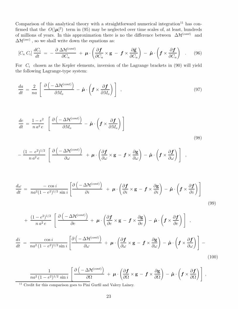
Comparison of this analytical theory with a straightforward numerical integration11 has con-firmed that the O(|µ|2) term in (95) may be neglected over time scales of, at least, hundredsof millions of years. In this approximation there is no the difference between ∆H(cont) and∆H(osc) , so we shall write down the equations as:

[Cn Ci]dCi

dt= − ∂ ∆H(cont)

∂Cn+ µ ·

(

∂f

∂Cn× g − f × ∂~g

∂Cn

)

− µ ·(

f × ∂f

∂Cn

)

. (96)

For Ci chosen as the Kepler elements, inversion of the Lagrange brackets in (90) will yieldthe following Lagrange-type system:

da

dt=

2

na

∂(

−∆H(cont))

∂Mo

− µ ·(

f × ∂f

∂Mo

)

, (97)

de

dt=

1 − e2

n a2 e

∂(

−∆H(cont))

∂Mo− µ ·

(

f × ∂f

∂Mo

)

(98)

− (1 − e2)1/2

n a2 e

∂(

−∆H(cont))

∂ω+ µ ·

(

∂f

∂ω× g − f × ∂g

∂ω

)

− µ ·(

f × ∂f

∂ω

)

,

dω

dt=

− cos i

na2(1 − e2)1/2 sin i

∂(

−∆H(cont))

∂i+ µ ·

(

∂f

∂i× g − f × ∂g

∂i

)

− µ ·(

f × ∂f

∂i

)

(99)

+(1 − e2)1/2

n a2 e

∂(

−∆H(cont))

∂e+ µ ·

(

∂f

∂e× g − f × ∂g

∂e

)

− µ ·(

f × ∂f

∂e

)

,

di

dt=

cos i

na2 (1 − e2)1/2 sin i

∂(

−∆H(cont))

∂ω+ µ ·

(

∂f

∂ω× g − f × ∂g

∂ω

)

− µ ·(

f × ∂f

∂ω

)

−

(100)

1

na2 (1 − e2)1/2 sin i

∂(

−∆H(cont))

∂Ω+ µ ·

(

∂f

∂Ω× g − f × ∂g

∂Ω

)

− µ ·(

f × ∂f

∂Ω

)

,

11 Credit for this comparison goes to Pini Gurfil and Valery Lainey.

23

dΩ

dt=

1

na2 (1 − e2)1/2 sin i

∂(

−∆H(cont))

∂i+ µ ·

(

∂f

∂i× g − f × ∂g

∂i

)

− µ ·(

f × ∂f

∂i

)

, (101)

dMo

dt= − 1 − e2

n a2 e

∂(

−∆H(cont))

∂e+ µ ·

(

∂f

∂e× g − f × ∂g

∂e

)

− µ ·(

f × ∂f

∂e

)

(102)

− 2

n a

∂(

−∆H(cont))

∂a+ µ ·

(

∂f

∂a× − f × ∂g

∂a

)

− µ ·(

f × ∂f

∂a

)

,

terms µ · ( (∂f/∂Mo) × g − (∂g/∂Mo) × f ) being omitted in (97 - 98), because these termsvanish identically (see the Appendix to Efroimsky (2004) ).

3.5 Comparison of calculations performed in the two above gauges

Simply from looking at (76 - 83) and (96 - 102) we notice that the difference in orbit descriptionsperformed in the two gauges emerges already in the first order of the precession rate µ andin the first order of µ .

Calculation of the µ- and µ-dependent terms emerging in (97 - 102) takes more than 20pages of algebra. The resulting expressions are published in Efroimsky (2005a), their detailedderivation being available in web-archive preprint Efroimsky (2004). As an illustration, wepresent a couple of expressions:

− µ ·(

f × ∂f

∂i

)

=

a2 (1 − e2)2

(1 + e cos ν)2 µ1 [ − cos Ω sin(ω + ν) − sin Ω cos(ω + ν) cos i ] sin(ω + ν)

+ µ2 [ − sin Ω sin(ω + ν) + cos Ω cos(ω + ν) cos i ] sin(ω + ν)

+ µ3 sin(ω + ν) cos(ω + ν) sin i , (103)

µ ·(

∂f

∂e× g − f × ∂~g

∂e

)

= − µ⊥

n a2 (3 e + 2 cos ν + e2 cos ν)

(1 + e cos ν)√

1 − e2, (104)

24

ν denoting the true anomaly. The fact that almost none of these terms vanish reveals thatequations (76 - 83) and (96 - 102) may yield very different results, i.e., that the contact elementsmay differ from their osculating counterparts already in the first order of µ .

Luckily, in the practical situations we need not the elements per se but their secular parts.To calculate these, one can substitute both the Hamiltonian variation and the µ- and µ-dependent terms with their orbital averages12 calculated through

〈 . . . 〉 ≡ (1 − e2)3/2

2 π

∫ 2π

0. . .

dν

(1 + e cos ν)2 . (105)

The situation might simplify very considerably if we could also assume that the precession rateµ stays constant. Then in equations (97 - 102), we would assume µ = const and proceedwith averaging the expressions ( (∂f/∂Cj) × g − f × (∂g/∂Cj) ) only (while all the termswith µ will now vanish).

Averaging of the said terms is lengthy and is presented in the Appendix to Efroimsky(2004). All in all, we get, for constant µ :

µ · 〈(

∂f

∂a× ~g − f × ∂g

∂a

)

〉 = µ ·(

∂f

∂a× ~g − f × ∂g

∂a

)

=3

2µ⊥

√

G m (1 − e2)

a, (106)

µ · 〈(

∂f

∂Cj

× g − f × ∂g

∂Cj

)

〉 = 0 , Cj = e , Ω , ω , i , Mo . (107)

Since the orbital averages (107) vanish, then e will, along with a , stay constant for as longas our approximation remains valid. Besides, no trace of µ will be left in the equations forΩ and i . This means that, in the assumed approximation and under the extra assumptionof constant µ , the afore quoted analysis (84 - 90), offered by Goldreich (1965), will remainvalid at time scales which are not too long.

In the realistic case of time-dependent precession, the averages of terms containing µ

and µ do not vanish (except for µ · ( (∂f/∂Mo) × g − f × (∂g/∂Mo) ) , which is identicallynil). These terms show up in all equations (except in that for a ) and influence the motion.Integration that includes these terms gives results very close to the Goldreich approximation(approximation (90) that neglects the said terms and approximates the secular parts of thenonosculating elements with those of their osculating counterparts). However, this agreementtakes place only at time scales of order millions to dozens of millions of years. At larger timescales, differences begin to accumulate (Lainey et al 2005).

In real life, the equinoctial-precession rate of the planet, µ , is not constant. Since theequinoctial precession is caused by the solar torque acting on the oblate planet, this precessionis regulated by the relative location and orientation of the Sun and the planetary equator. Thisis why µ of a planet depends upon this planet’s orbit precession caused by the pull from theother planets. This dependence is described by a simple model developed by Colombo (1966).

12 Mathematically, this procedure is, to say the least, not rigorous. In practical calculations it works well, atleast over not too long time scales.

25

4 Conclusions: how we benefit from the gauge freedom.

In this article we gave a review of the gauge concept in orbital and attitude dynamics. Essen-tially, this is the freedom of choosing nonosculating orbital (or rotational) elements, i.e., thefreedom of making them deviate from osculation in a known, prescribed, manner.

The advantage of elements introduced in a nontrivial gauge is that in certain

situations the choice of such elements considerably simplifies the mathematical

description of orbital and attitude problems. One example of such simplification is theGoldreich (1965) approximation (90) for satellite orbiting a precessing oblate planet. Althoughperformed in terms of non-osculating elements, Goldreich’s calculation has the advantage ofmathematical simplicity. Most importantly, later studies (Efroimsky 2005a,b) have confirmedthat Goldreich’s results, obtained for nonosculating elements, serves as a very good approxi-mation for the osculating elements. To be more exact, the secular parts of these nonosculatingelements coincide, in the first order over the precession-caused perturbation, with those of theirosculating counterparts, the difference accumulating only at very long time scales – see the endof section 3 above. A comprehensive investigation into this topic, with the relevant numerics,will be presented in Lainey et al (2005).

On the other hand, neglect of the gauge freedom may sometimes produce camou-

flaged pitfalls caused by the fact that nonosculating elements lack evident physical

meaning. For example, the nonosculating “inclination” does not coincide with the real, physi-cal inclination of the orbit. This happens because nonosculating elements parameterise instan-taneous conics nontangent to the orbit. Similarly, nonosculating Andoyer elements L , G , Hare no longer the same projections of the angular momentum as their osculating counterparts.

Appendix 1. Mathematical formalities:

Orbital dynamics in the normal form of Cauchy

Let us cast the perturbed equation

r = F + ∆f = − µ

r2

r

r+ ∆f (108)

into the normal form of Cauchy:

r = v , (109)

v = − µ

r2

r

r+ ∆f ( r(t , C1 , ... , C6) , v(t , C1 , ... , C6) , t ) . (110)

Insertion of our ansatz

r = f ( t , C1(t) , . . . , C6(t) ) , (111)

will make (109) equivalent to

v =∂f

∂t+∑

i

∂f

∂CiCi . (112)

26

The function f is, by definition, the generic solution to the unperturbed equation

r = F = − µ

r2

r

r. (113)

This circumstance, along with (112), will transform (109) into

∑

i

∂g

∂Ci

Ci + Φ = ∆F ( f (t , C1 , ... , C6) , g(t , C1 , ... , C6) + Φ ) (114)

where

Φ ≡∑

i

∂f

∂CjCj (115)

is an identity, f (t , C1 , ... , C6) and g(t , C1 , ... , C6) ≡ ∂f/∂t being known functions. Now(114 - 115) make an incomplete system of six first-order equations for nine variables (C1 , ... , C6 ,Φ1 , ... , Φ3) . So one has to impose three arbitrary conditions on C , Φ , for example as

Φ = Φ( t , C1 , ... , C6 ) . (116)

This will result in a closed system of six equations for six variables Cj :

∑

i

∂g

∂CiCi = ∆F ( f (t , C1 , ... , C6) , g(t , C1 , ... , C6) + Φ ) − Φ (117)

∑

i

∂f

∂Ci

dCi

dt= Φ , (118)

Φ = Φ( t , C1 , ... , C6 ) now being some fixed function (gauge).13 A trivial choice isΦ( t , C1 , ... , C6 ) = 0 , and this is what is normally taken by default. This choice is onlyone out of infinitely many, and often is not optimal. Under an arbitrary, nonzero, choice of thefunction Φ( t , C1 , ... , C6 ) , the system (117 - 118) will have some different solution Cj(t) .To get the appropriate solution for the Cartesian components of the position and velocity, onewill have to use formulae

r = f ( t , C1 , ... , C6 ) , (119)

r ≡ v = g( t , C1 , ... , C6 ) + Φ( t , C1 , ... , C6 ) , (120)

13 Generally, Φ may depend also upon the variables’ time derivatives of all orders: Φ(t; Ci , Ci , Ci , ...).This will give birth to higher time derivatives of C in subsequent developments and will require additionalinitial conditions, beyond those on r and r , to be fixed to close the system. So it is practical to accept (116).

27

Appendix 2. Precession of the equator of date

relative to the equator of epoch

The afore introduced vector µ is the precession rate of the equator of date relative tothe equator of epoch. Let the inertial axes ( X , Y , Z ) and the corresponding unit vectors( X , Y , Z ) be fixed in space so that X and Y belong to the equator of epoch. A rotationwithin the equator-of-epoch plane by longitude hp , from axis X , will define the line of nodes,x . A rotation about this line by an inclination angle Ip will give us the planetary equatorof date. The line of nodes x , along with axis y naturally chosen within the equator-of-dateplane, and with axis z orthogonal to this plane, will constitute the precessing coordinatesystem, with the appropriate basis denoted by ( x , y , z ) .

In the inertial basis ( X , Y , Z ) , the direction to the North Pole of date is given by

z = ( sin Ip sin hp , − sin Ip cos hp , cos Ip )T

(121)

while the total angular velocity reads:

ω(inertial)total = z Ωz + µ(inertial) , (122)

the first term denoting the rotation about the precessing axis z , and the second term beingthe precession rate of z relative to the inertial frame ( X , Y , Z ) . This precession rate isgiven by

µ(inertial) =(

Ip cos hp , Ip sin hp , hp

)T

, (123)

because this expression satisfies µ(inertial) × z = ˙z .In a frame co-precessing with the equator of date, the precession rate will be represented

by vector

µ = Ri→p µ(inertial) , (124)

where the matrix of rotation from the equator of epoch to that of date (i.e., from the inertialframe to the precessing one) is given by

Ri→p =

cos hp sin hp 0

− cos Ip sin hp cos Ip sin hp sin Ip

sin Ip sin hp − sin Ip sin hp cos Ip

From here we get the components of the precession rate, as seen in the co-precessing coordinateframe (x , y , z) :

µ = ( µ1 , µ2 , µ3 )T

=(

Ip , hp sin Ip , hp cos Ip

)T

. (125)

28

References

[1] Berkovich, L. M. 2002. “Research of Non-Stationary Problems of Celestial Mechanics Trans-formation to an Autonomous Form.” In: Non-Stationary Dynamical Problems in Astronomy.Collection of articles, ed. by T. B. Omarov. Nova Science Publishers, New York, 2002.

[2] Brumberg, V. A., L. S. Evdokimova, & N. G. Kochina. 1971. “Analytical Methods for theOrbits of Artificial Satellites of the Moon.” Celestial Mechanics, Vol. 3, pp. 197 - 221.

[3] Colombo, G. 1966. “Cassini’s second and third laws.” The Astronomical Journal., Vol. 71

pp. 891 - 896.

[4] Efroimsky, Michael. 2002a. “Equations for the orbital elements. Hidden symmetry.”Preprint 1844 of the Institute of Mathematics and its Applications, University of Minnesotahttp://www.ima.umn.edu/preprints/feb02/feb02.html

[5] Efroimsky, Michael. 2002b. “The Implicit Gauge Symmetry Emerging in the N-body Prob-lem of Celestial Mechanics.” astro-ph/0212245

[6] Efroimsky, Michael, & Peter Goldreich. 2003. ”Gauge Symmetry of the N-body Problem inthe Hamilton-Jacobi Approach.” Journal of Mathematical Physics, Vol. 44, pp. 5958 - 5977astro-ph/0305344

[7] Efroimsky, Michael, & Peter Goldreich. 2004. ”Gauge Freedom in the N-body Problem ofCelestial Mechanics.” Astronomy & Astrophysics, Vol. 415, pp. 1187 - 1199astro-ph/0307130

[8] Efroimsky, M. 2004. “Long-term evolution of orbits about a precessing oblate planet. Thecase of uniform precession.” astro-ph/0408168This preprint is a very extended version of the published paper Efroimsky (2005). It containsall technical calculations omitted in the said publication.

[9] Efroimsky, M. 2005a. “Long-term evolution of orbits about a precessing oblate planet. 1.The case of uniform precession.” Celestial Mechanics and Dynamical Astronomy, Vol. 91,pp. 75 - 108

[10] Efroimsky, M. 2005b. “Long-term evolution of orbits about a precessing oblate planet. 2.The case of variable precession.” In preparation.

[11] Euler, L. 1748. Recherches sur la question des inegalites du mouvement de Saturne et deJupiter, sujet propose pour le prix de l’annee. Berlin. Modern edition: L. Euler Operamechanica et astronomica. Birkhauser-Verlag, Switzerland, 1999.

[12] Euler, L. 1753. Theoria motus Lunae exhibens omnes ejus inaequalitates etc. ImpensisAcademiae Imperialis Scientarum Petropolitanae. St.Petersburg, Russia 1753. Modernedition: L. Euler Opera mechanica et astronomica. Birkhauser-Verlag, Switzerland 1999

[13] Fukushima, T., & Ishizaki, H. 1994. “Elements of Spin Motion.” Celestial Mechanics andDynamical Astronomy, Vol. 59, pp. 149 - 159.

[14] Goldreich, P. 1965. “Inclination of satellite orbits about an oblate precessing planet.” TheAstronomical Journal, Vol. 70, p. 5 - 9

29

[15] Gurfil, P., and Klein, I. 2006. “Mitigating the Integration Error in Numerical Simulationsof Newtonian Systems.” Submitted to The International Journal for Numerical Methods inEngineering.

[16] Gurfil, P. 2004. “Analysis of J2−perturbed Motion using Mean Non-Osculating OrbitalElements.” Celestial Mechanics & Dynamical Astronomy, Vol. 90, pp. 289 - 306

[17] Kinoshita, T. 1993. “Motion of the Orbital Plane of a Satellite due to a Secular Changeof the Obliquity of its Mother Planet.” Celestial Mechanics and Dynamical Astronomy, Vol.57, pp. 359 - 368

[18] Lagrange, J.-L. 1778. Sur le Probleme de la determination des orbites des cometes d’aprestrois observations, 1-er et 2-ieme memoires. Nouveaux Memoires de l’Academie de Berlin,1778. Later edition: Œuvres de Lagrange. Vol. IV, Gauthier-Villars, Paris 1869.

[19] Lagrange, J.-L. 1783. Sur le Probleme de la determination des orbites des cometes d’aprestrois observations, 3-ieme memoire. Ibidem, 1783. Later edition: Œuvres de Lagrange.Vol. IV, Gauthier-Villars, Paris 1869.

[20] Lagrange, J.-L.1808. “Sur la theorie des variations des elements des planetes et en par-ticulier des variations des grands axes de leurs orbites”. Lu, le 22 aout 1808 a l’Institut deFrance. Later edition: Œuvres de Lagrange.Vol.VI, pp.713-768, Gauthier-Villars, Paris 1877

[21] Lagrange, J.-L. 1809. “Sur la theorie generale de la variation des constantes arbitrairesdans tous les problemes de la mecanique”. Lu, le 13 mars 1809 a l’Institut de France. Lateredition: Œuvres de Lagrange.Vol.VI, pp.771-805, Gauthier-Villars, Paris 1877.

[22] Lagrange, J.-L.1810. “Second memoire sur la theorie generale de la variation des constantesarbitraires dans tous les problemes de la mecanique”. Lu, le 19 fevrier 1810 a l’Institut deFrance. Later edition: Œuvres de Lagrange. Vol.VI, pp.809-816, Gauthier-Villars, Paris 1877

[23] Lainey, V.; Gurfil, P.; & Efroimsky, M. 2005. “Long-term evolution of orbits about aprecessing oblate planet. 3. A semianalytical and a purely numerical approaches.”In preparation.

[24] Mysen, E. 2004. “Rotational dynamics of subsolar sublimating triaxial comets,” Planetaryand Space Science, Vol. 52, pp. 897 - 907.

[25] Newman, W., & M. Efroimsky. 2003. “The Method of Variation of Constants and MultipleTime Scales in Orbital Mechanics.” Chaos, Vol. 13, pp. 476 - 485.

[26] Plummer, H. C. 1918. An Introductory Treatise on Dynamical Astronomy. CambridgeUniversity Press, UK.

[27] Slabinski, V. 2003. ”Satellite Orbit Plane Perturbations Using an Efroimsky Gauge Ve-locity.” Talk at the 34th Meeting of the AAS Division on Dynamical Astronomy, CornellUniversity, May 2003.

[28] Zanardi, M. C.; Vilhena de Moraes, R. 1999. “Analytical and semi-analytical analysis ofan artificial satellite’s rotational motion.” Celestial Mechanics and Dynamical Astronomy,Vol. 75, pp. 227 - 250.

30