Gasoline Price Differences: Taxes, Pollution Regulations, Mergers, Market Power, and Market Conditions

Hayley Chouinard* Jeffrey M. Perloff**

September 2002

Abstract

Retail and wholesale gasoline prices vary over time and across geographic locations due to differences in government policies and other factors that affect demand, costs, and market power. We use a two-equation, reduced-form model to determine the relative importance of these various factors. An increase in the price of crude oil has been virtually the only major factor contributing to a general rise in prices over the last couple of decades. Tax variations and mergers contribute substantially more to geographic price differentials than do price discrimination, cost factors, or pollution controls. * Assistant Professor, Department of Agricultural and Resource Economics, Washington State

University. ** Professor, Department of Agricultural and Resource Economics, University of California,

Berkeley, and member of the Giannini Foundation. The authors thank Severin Borenstein, Jeffrey LaFrance, and Michael Ward for their considerable help.

Table of Contents

1. Introduction ............................................................................................................................ 1

2. A Reduced-Form Gasoline Price Model............................................................................... 2

2.1. Demand................................................................................................................................ 4

2.2. Costs .................................................................................................................................... 5

2.3. Seasonality........................................................................................................................... 6

2.4. Market Power ...................................................................................................................... 7

2.5. Taxes.................................................................................................................................... 9

2.6. Anti-Pollution Laws .......................................................................................................... 10

2.7. Vertical Relations .............................................................................................................. 11

3. National Price Trends............................................................................................................ 12

4. Differences in Prices across States........................................................................................ 13

4.1. Retail Price Effects ............................................................................................................ 14

4.2. Wholesale Price Effects..................................................................................................... 15

4.3. Comparison Across Specific States ................................................................................... 16

5. Conclusions ............................................................................................................................. 16

Appendix ...................................................................................................................................... 22

1. Introduction

Politicians, newspapers, and annoyed motorists throughout the United States question

why gasoline prices rise and why gasoline prices are substantially greater in some areas than

others. We assess the degree to which many proposed explanations cause retail and wholesale

gasoline price changes and price differentials.

An extremely vocal debate on gasoline prices arose during the 2000 presidential election

year. House Speaker Dennis Hastert and other Republicans blamed Environmental Protection

Agency (EPA) policies for soaring gas prices in the Midwest.1 Many Democrats alleged the

major oil company price fixing was responsible for the increases and that only a 4 to 8¢ a gallon

rise was due to EPA rules.

The California Service Station and Automotive Repair Association claimed that motorists

in the Bay Area pay more for gas than do those in Los Angeles due to wholesale “zoned

pricing,” which Chevron, Arco and other oil companies acknowledged they use.2 According to

these dealers, the price differences reflect price discrimination rather than cost differences.

Indeed, a Chevron spokesperson stated:3

We price each market to be competitive. In a metropolitan area, there may be pockets where prices are higher or lower than other pockets. It’s not based on our costs but on the market in that area.

1 “Hastert Accuses EPA of Scapegoating Oil Companies,” San Francisco Chronicle, July 15, 2000: A3.

2 Howe, Kenneth, “Bay Area Pays More for Gas,” San Francisco Chronicle, May 9, 1997: A1,

A17. 3 Platt’s Oilgram News, June 3, 1997.

2

According to Richard Parker, director of the Federal Trade Commission’s Bureau of

Competition, consumers across the entire west coast face zone pricing and “redlining.”4

Redlining occurs when independent distributors are prohibited from selling branded gasoline. A

report by California’s attorney general attributed high prices in California to a lack of

competition in certain areas, the state’s strict clean-air standards, and high taxes.5

In the next section, we describe our estimated reduced-form model, which shows how

retail and wholesale prices vary with demand, cost, seasonal factors, taxes, market power,

pollution controls, and government restrictions on vertical integration. So far as we know, this

paper is the first to assess the impact of a wide variety of factors on pricing (we briefly discuss

other papers that analyze the impact of one or a few factors on pricing). In Section 3, we

examine which factors were primarily responsible for price increases over the last decade. We

analyze which factors cause geographic price differentials in Section 4. In the last section, we

summarize our results and draw conclusions.

2. A Reduced-Form Gasoline Price Model

To examine the relative importance of various factors that affect gasoline prices by state

and over time, we use a reduced-form model, which is consistent with both competitive and

noncompetitive behavior. For example, suppose the underlying model is a standard, market-

level model of a potentially noncompetitive market. Let Q be demand, p be price, X be the

4 Rivera, Nancy Brooks, “Regulators Find Redlining, Zone Pricing of Fuel,” Los Angeles Times, September 27, 2000, C1.

5 Gledhill, Lynda, “California’s High Gas Prices Look to Be Legal,” San Francisco Chronicle,

November 23, 1999, A3.

3

exogenous demand shifters, W be the exogenous cost shifters, Z be exogenous market power

shifters, and let v(Z) measure the degree of market power (ranging from competitive to

monopoly). The demand equation is Q = D(p, X), the marginal cost equation is MC(W), and the

market-level “optimality” equation (MR = MC) implies that p = (v(Z), X, W). We estimate the

reduced-form specification, p = f(X, W, Z), which holds for any market structure (v).6

We estimate reduced-form wholesale and retail gasoline price equations using monthly

panel data for 48 states (all but Alaska and Hawaii) and the District of Columbia from January of

1989 through June of 1997. We group the factors that affect gasoline prices into seven

categories: demand, cost, seasonality (which affects both demand and cost), market power, taxes,

pollution laws, and vertical relations (which affect market power and cost). Due to the vertical

nature of the wholesale and retail markets, the inverse demand function of the wholesale market

depends on the marginal revenue function of the retail market. Thus, the reduced-form equations

for retail and wholesale gasoline include the same variables.

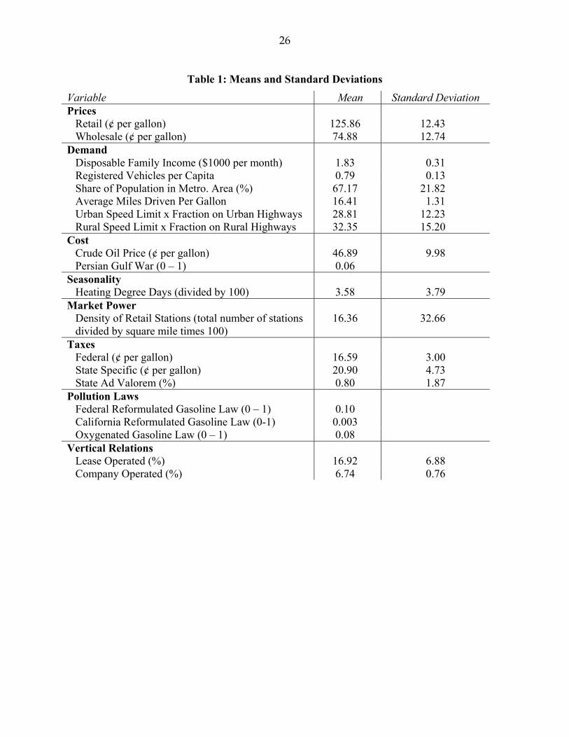
In the regressions, all monetary variables are measured in 1997 (real) dollars. The

Appendix describes the data and sources. Table 1 lists our variables, their units of

measurement, their means, and their standard deviations (for the continuous variables).

We estimate linear, fixed-effects equations to explain why prices vary over time and

across states.7 The equations do not suffer from multicollinearity problems.8 The estimated

6 We could, in principle, estimate this structural model. However, due to inadequate variation in the data, we could not estimate stable and plausible state-specific demand curve. Consequently, we estimate the reduced-form model.

7 We also experimented with other data sets and specifications: We used a city (rather than

state) database, we examined semi-log and log-log specifications, and we substituted the wholesale price for the crude oil price on the right-hand side of the retail-price equation. Each of these alternative models produced qualitatively (and usually quantitatively) similar results to

4

equations fit the price data closely: The R2 is 0.90 in the retail-price equation and 0.89 in the

wholesale-price equation. Table 2 reports the estimated reduced-form coefficients (except for 35

merger dummy coefficients, 11 monthly dummies, and 49 fixed effect dummies) for the retail-

price and wholesale-price equations.

2.1. Demand

The effect of a shift in the demand curve on prices depends on costs and market structure.

If gasoline markets are competitive and the gasoline supply curve is upward sloping, a right shift

of the demand curve causes gasoline prices to rise. However, if wholesalers and retailers are

price setters, an outward shift of the demand curve may, but does not necessarily lead to higher

prices. Further, a factor that varies across states causing differences in demand elasticities may

lead to price discrimination if firms have market power. The variables that presumably affect

demand include average state income, the number of registered vehicles per capita, the fraction

of the state’s population that lives in a metropolitan area, the fuel-efficiency of vehicles in a

state, and urban and rural speed limits.

those reported here. We use a fixed-effect model because we have an exhaustive sample of the mainland states. We rejected the hypothesis of a random-effects model based on Hausman model-specification tests: the p-values are 0.0 for the Chi-squared test statistic for both the retail and wholesale equations.

8 The regressions were estimated using standard orthonormalized data matrices to compensate

for possible multicollinearity. There is relatively little correlation between most pairs of the explanatory variables (except between various degrees of lags of crude oil prices). We re-estimated a set of equations without the share of population in a metroloitan area and the density of retail stations, which are the variables with the highest correlation with the several other variables and found little change in the remaining coefficients.

5

Because previous researchers found that gasoline is a normal good, we expect an increase

in per capita income to shift the demand curves for gasoline to the right.9 The per capita income

variable is not statistically significantly different from zero in both the retail-price and

wholesale-price equations. The number of registered vehicles per capita, the fraction of people

living in metropolitan areas, and the average miles per gallon do not have a significant effect on

retail or wholesale prices.

The amount of gasoline used depends on the speed limit. Our urban and rural interstate

speed limits variables are the interaction of the maximum posted speed times the fraction of total

interstate miles driven on urban or rural interstates respectively. The Department of

Transportation defines urban and rural interstates depending on their proximity to population

centers. The urban limit is not statistically significant in the wholesale equation. However, it is

positive and significant in the retail equation. The rural variable is statistically significant in

both equations. Increasing the rural speed limit by one mile per hour will decrease the retail

price by .21¢ and the wholesale price by .07¢ respectively, multiplied by the fraction of interstate

miles drive on rural interstates in a given state.

2.2. Costs

The major cost variables are the price of crude oil and a Persian Gulf War dummy. The

most important input in the production of gasoline is crude oil.10 To capture possible lags in

9 In Dahl and Sterner’s (1991) survey of over a hundred gasoline demand studies, the short-run income elasticity ranged from 0.14 to 0.58 and the long-run income elasticity ranged from 0.60 to 1.31.

10 According to the Petroleum Supply Annual, Volume 2, the United States gasoline imports are

only between 3% and 4% of the amount of gasoline produced domestically. Moreover, only 2.5% - 3.5% of gasoline imports originate in countries that also export crude oil to the United

6

adjustment or adaptive expectations about crude oil prices, we include the current crude oil price

and two lags.11 (If we include one more lag, we cannot reject that its coefficient is zero in either

equation.) These coefficients are collectively statistically significant in each equation and five of

the six coefficients are individually significant at the 0.05 level. The sum of the three

coefficients in each equation equals almost exactly one. Thus, a permanent increase in the price

of crude oil raises the wholesale and retail prices by virtually the same amount.

We use a dummy that equals one during the Persian Gulf War (January through June

1991) to capture increases in cost from maintaining larger inventories of crude oil and gasoline

due to increased uncertainty about deliveries. This effect is statistically significant in both

equations. During the war, retail prices increased by 1.7¢ per gallon and wholesale prices

increased by 3.0¢ per gallon. (If we include an extra one or two months prior and after the

Persian Gulf War in our dummy, our results are virtually unchanged.)

2.3. Seasonality

Both demand and cost vary with temperature and over seasons. Demand curves shift to

the right in warmer, summer months when more trips are taken. Because the demand for home

heating oil rises during cold weather, refineries produce more home heating oil then and more

gasoline (which is produced jointly with heating oil). We include the number of heating degree-

days as well as monthly dummy variables (December is the base month) to capture temperature

States during our time period. Thus, we did not include a measure of imported gasoline in our equation.

11 Borenstein and Shepard (2000) conclude that firms vary wholesale prices slowly in respond to

crude oil price changes to reduce production and inventory adjustment costs. They report that firms with high price-cost margins adjust wholesale prices more slowly than do more competitive firms.

7

and seasonal effects.12 Most of the monthly dummies and the heating degree-day variables are

statistically significantly different from zero. Going from no heating degree-days to 100 in a

month causes the retail price to fall by 0.21¢ and the wholesale price to drop by 0.24¢. The

largest price differences due to seasonality occur in May for the wholesale price (prices are 8.5¢

higher than in December) and June for the retail price (prices are 5.7¢ higher).

2.4. Market Power

Gasoline manufacturers and retailers may have market power.13 Figure 1 shows that the

national markup of the retail price over the wholesale price and the markup of the wholesale

price over the crude oil price vary over time. Mergers and changes in the density of gas stations

affect market power over time.

Mergers and divestitures (henceforth “mergers” for short) either lower prices by

increasing efficiency or raise prices by enhancing market power. Although no large, national

merger occurred during our sample period, there were 8 producer mergers in 5 states and 27

retail mergers in 19 states. We capture these mergers for the affected states using a dummy that

equals zero prior to the merger and one thereafter. In the retail-price equation, the retail merger

dummies had 10 positive coefficients (5 statistically significant) and 17 negative coefficients (8),

12 The heating degree-days measure is the total number of average daily degrees below 65 that occurs each month (National Oceanic and Atmospheric Administration, 1989-1997). For example, if the highest daily temperature in a month was 50° one day, 52° a second day, and at least 65° every other day in that month, then the total heating degree-days for that month is 28 = (65 – 50) + (65 – 52). In our regressions, we normalize the degree-days by dividing by 100.

13 Refiners implicitly admit they have market power by openly discussing their ability to price

discriminate. Several academic articles contend that gasoline retailers have market power, which they use to price discriminate (Slade, 1986; Borenstein, 1991; Shepard, 1991; Borenstein and Shepard, 1996). However, Marvel (1978) concludes that prices are not above competitive

8

and the producer merger dummies had 5 positive coefficient (1) and 3 negative coefficients (1).14

In the wholesale price equation, there were 6 positive retail merger coefficients (2 statistically

significant) and 21 negative retail-merger coefficients (4), 5 positive wholesale-merger

coefficient (2), and 3 negative wholesale-merger coefficients (1).15

Marvel (1976) concluded that imperfect price information accounted for some of the retail

gasoline price dispersion within a geographic area and through time. Because of travel costs,

consumers tend to limit their price search for inexpensive gasoline to their immediate area. As a

result, we might expect that stations can exercise more market power, the fewer the retail gas

stations per square mile. As the number of stations per square mile increases by one percentage

point, the retail price falls by a statistically insignificant 0.01¢. This variable does not have a

statistically significant effect in the wholesale price equation either.

levels because consumers are well informed and have relatively elastic demands for gasoline which makes it difficult for retailers to collude.

14 The largest statistically significant coefficient for a retail merger involved Giant Industries Inc.

in Arizona in 1993. The most negative significant coefficient was for the 1995 Arizona retail merger when Midway Oil purchased Kerr-McGee Rio Grande Valley. The largest statistically significant coefficient in the wholesale equation reflects the effect of the 1992 California merger between Fletcher Oil and Signal Hill Petroleum Inc. The largest negative producer merger occurred in Louisiana in 1995 when Calumet Lubricants Company took over Kerr McGee-Cotton Valley.

15 In general, the same mergers that had large effects in the retail price equation also had the

major effects in the wholesale equation. The one exception is the 1995 Arizona sale by Exxon Co. USA of 83 stations to Tosco Corporation, which had the largest negative effect in the retail regression but was not important in the wholesale equation.

9

2.5. Taxes

Federal and state governments apply specific gasoline taxes. During the sample period,

the federal specific tax ranged from between nearly 11¢ and 20¢ per gallon. The state-specific

taxes varied from 7¢ to 36¢ per gallon.

The incidence of federal specific tax is substantially different from that of state specific

taxes. When the federal specific tax increases by one cent, the retail price rises by about half a

cent and the wholesale price drops by about one half a cent. Thus, retail consumers pay half the

tax, wholesalers absorb half the tax, and retailers bear none of the tax incidence.

When a state increases its specific tax by 1¢, the incidence of the tax falls almost entirely

on consumers: The retail price rises by 1¢ and the wholesale price remains essentially constant.

Thus, a change in one state’s specific tax causes the retail price in that state to rise relative to

prices in other states by nearly the amount of the tax. Possibly arbitrage across states explains

why producers absorb none of the state specific taxes, whereas they pay for half of the federal

tax.

Only California, Georgia, Illinois, Indiana, Louisiana, Michigan, Mississippi, and New

York apply ad valorem taxes to the retail gasoline price. Ad valorem tax rates range up to 7

percent of the retail price (which includes the specific taxes). Raising the ad valorem tax rate

from 0 to 5% raises the retail price by 8.7¢ and has no significant effect on wholesale prices. 16

16 Although it is unclear how best to specify the effects of an ad valorem tax rate in these equations, the qualitative results are not very sensitive to changes in the specification such as using the log of the ad valorem rate.

10

2.6. Anti-Pollution Laws

Some governments require produces to modify gasoline formulations to control pollution.

These restrictions affect market power, efficiency, or both.

Two anti-pollution measures affect costs and market power. The 1990 Clean Air Act

Amendment requires certain regions to use special formulations of gasoline at specific times to

reduce the pollution generated by gasoline combustion. Starting in January 1993, these

regulations required the exclusive, year-round use of reformulated gasoline in some major cities

across a number of states. Starting in October 1991, several states required that only oxygenated

gasoline be sold during winter months in some of their major cities. The Appendix lists the

states that required the use of oxygenated and reformulated gasoline during the sample period.

The requirement that stations sell only specially formulated pollution-reducing gasoline

increases refining costs and may create market power for wholesalers within a state. To produce

reformulated gasoline, refiners must make several costly modifications to their production

equipment. If producers in surrounding states avoid incurring these large capital costs, producers

in states mandating the use of reformulated or oxygenated gas do not face competition from

these out-of-state suppliers. The federal reformulation regulation increases the retail price by .8¢

and does not have a statistically significant effect in the wholesale equation.

California is the only state with its own reformulated gasoline law. Some industry

experts have argued that California’s reformulation law has had a large effect on that state’s

prices. We include a dummy variable that equals one beginning in March 1996 when California

first began production of its reformulated gasoline. This regulation raised retail prices in

11

California by 3.9¢ but did not have a statistically significant effect on the wholesale price.17 In a

month when gasoline must be oxygenated, the retail price rises by 3.7¢ and the wholesale price

increases by 2.9¢.

2.7. Vertical Relations

Many politicians contend that vertical relations between refiners and retailers affect

market power. Whether producers are vertically integrated may also affect costs. Gilbert and

Hastings (2001) find that an increase in the degree of vertical integration between gasoline

refiners and distributors is associated with higher wholesale prices. Thus, contractual

arrangements between retailers and producers may affect prices.

There are three types of retail stations. First, a brand-name producer (such as Shell or

Exxon) may vertically integrate into retailing, where its stations sell only the brand-name

gasoline at a price determined by the manufacturer. Second, a lease contract restricts the lessee

to sell only the manufacturer’s brand of gasoline and dictates many operational decisions, but the

lessee determines the retail price. Third, open dealers may agree to sell a specific brand of

gasoline, but the dealers make all operational and pricing decisions.

To capture the effects of vertical relations, we include the national share of producer-

operated brand-name retail outlets and the share of retail outlets leased from producers.

17 The California price differential may rise due to a recent court decision concerning reformulated gasoline. Before California’s stricter reformulated gasoline requirements went into effect, Unocal patented the cleaner burning fuel that all companies use. A federal appeals court upheld the patent in March 2000. Six major oil companies paid Unocal 5.75¢ a gallon on 1.2 billion gallons of patent-infringing reformulated gasoline produced during a five-month period in 1996 after they lost their appeal. Since then, Unocal has been in repeated court battles over its patents, and has lost many of these cases.

12

Unfortunately, we know the share of branded retail stations operated with a lease contract or by

an integrated firm only at the national level.

The base category is the share of open stations. Because the coefficients on the share of

company-run stations are not statistically significantly different from zero but the share of leased

stations has positive, statistically significantly coefficients in both equations, we infer that prices

rise when the share of such stations increases. A possible alternative explanation is that this

relationship is due to the selection criterion that manufacturers use in deciding which stations to

operate under lease contracts.

3. National Price Trends

The crude oil price, Gulf War dummy, monthly dummies (which capture seasonal effects

other than those due to temperature), and share of leased and company operated stations

variables do not vary across states and hence cannot explain cross-state price variations but can

contribute to national price trends. Of our national variables, only the price of crude oil trended

over our sample period. Consequently, it was the only national variable that contributed to the

upward trend in retail and wholesale prices.

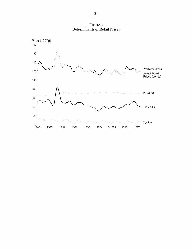
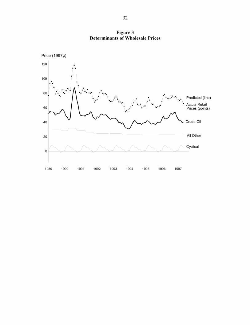
Figures 2 and 3 show our estimates of the relative impacts of various factors (evaluated at

their national means) on wholesale and retail prices. In each figure, the predicted price line is

closely surrounded by the dots reflecting actual prices. The “crude-oil” line shows the impact of

the crude oil price (and its lags) on predicted retail- and wholesale gasoline prices. Crude oil

accounts for 62 percent of the predicted wholesale price and for 37 percent of the predicted retail

price. The retail- and wholesale-price lines are virtually parallel to the crude-oil price line

because the effects of other variables are nearly constant when averaged over a year.

13

In each figure, the “cyclical” line reflects the effects of variables that cycle over the year:

the heating degree-days, the requirement to oxygenate gasoline, and the monthly dummies. The

“all other” line reflects the effects of other variables (taxes, Gulf War dummy, and other state-

specific variables). This line is virtually horizontal, which is not surprising because most of

these variables primarily vary across states rather than over time. Thus, virtually the entire

variation in national prices was due to changes in the crude oil price and cyclical fluctuations,

and not to changes in taxes, pollution laws, and other factors.

4. Differences in Prices across States

We now examine which factors cause retail and wholesale gasoline prices to vary across

states. The larger a variable’s coefficient and the larger is its average value, the greater is this

variable’s average effect on prices. However, whether this variable causes substantial

geographic differences depends on the range of values for this variable across states.

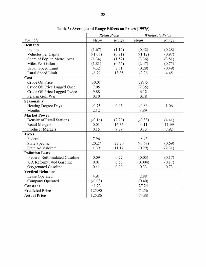
Table 3 shows the average national effect and the range of effects across states for each

variable in each equation. (Numbers in parentheses are based on coefficients that are not

statistically significantly different from zero.) For example, the columns labeled “mean” show

that income (first row) contributes 1.7¢ to the retail price and 0.4¢ to the wholesale price at

national average levels. The “range” columns show how much of the variation in prices across

states is explained by income.18

18 We multiply the absolute value of the variable’s estimated coefficient times the range in (the average) values of this variable across states. For the reformulated gasoline and oxygenated gasoline law dummies, we take the absolute value of the product of the coefficient and the average value of the dummy over the year (for example, the oxygenated gasoline dummy equals one only during the winter months when the oxygenated gasoline is required in each state). Consequently, all the numbers in these columns are positive.

14

4.1. Retail Price Effects

Crude oil and taxes had the largest average price effects. The crude oil price contributed

over 46¢ (the sum of the level and two lag effects) on average to both the retail and wholesale

prices. The federal specific tax added 8¢ on average to retail price, but lowered the wholesale

price by nearly 9¢. The mean state specific tax contributed 20.3¢ to the retail price but

essentially did not affect the wholesale price. Because few states apply ad valorem taxes to

gasoline, these taxes had relatively little impact on the national average, 1.4¢.

Of the demand variables, only the speed limit measures significantly affect prices. The

urban speed limit measure increased the retail price by 4.3¢. The rural speed limit measure

lowered the retail price by 6.8¢ and the wholesale price by 2.3¢.

The vertical relations variable of the percent of lease operated retail outlets significantly

affects retail and wholesale prices. A 1% increase in the number of leased stations increases the

retail price by 4.9¢ and the wholesale price by 2.9¢.

Even though a variable has a large average effect on prices, it may not explain much of

the variation in retail prices across the country. For example, the crude oil price cannot explain

the cross-state range in prices because it does not vary across states.

State specific taxes had the largest impact on interstate retail price differentials. All else

the same, state specific taxes explained up to 22.2¢ of the difference in retail prices across states.

Georgia had the lowest specific tax of 8.4¢ and Connecticut the highest, 31.3¢. Consumers in

Mississippi with a high ad valorem tax rate of 6.42 percent (averaged over the sample period),

paid 11.1¢ more at retail.

15

Retail mergers created up to a 16.4¢ retail price differential across states, whereas

producer mergers caused a maximum retail price difference of 9.8¢.19 A 1993 Arizona merger

had the largest effect, increasing that state’s retail price by nearly 9¢. A 1995 merger decreased

the retail price in California by 7.5¢. A 1992 manufacturers’ merger increased California retail

prices by 8.7¢. A 1995 Louisiana merger decreased retail prices in that state by about 3¢.

The urban speed limit measure accounts for 7.3¢ in retail price differences. The rural

speed limit measure explained up to a 13.4¢ differential in retail prices. Pollution laws that

require different forms of gasoline be sold raised the retail price from .3¢ to .9¢ (taking account

of the share of the year the laws are in effect).

The other state-specific variables did not have a statistically significant effect on the retail

price. The point estimates for these variables are small.

4.2. Wholesale Price Effects

The factors that were most important in explaining wholesale price variations differed

somewhat from those that explain retail patterns. Mergers had the largest impact on wholesale

prices. The largest effect was a nearly 7¢ wholesale price increase due to a 1993 Arizona retail

merger. The retail merger in Arizona in 1995 reduced the wholesale price in Arizona by over

5¢. The 1992 California producer merger increased that state’s wholesale price by 5.8¢. The

1995 Louisiana producer merger reduced its wholesale price by 2¢.

The rural speed limit measure causes wholesale prices to differ by 4.5¢. Temperature

differences (heating degree-days) accounted for up to a 1.1¢ differential. Oxygenated gasoline

19 To calculate the price differential between states with mergers and those without, we take the absolute value of the largest merger coefficient. (Alternatively, we could have compared mergers with positive price effects to those with negative price effects.)

16

laws raised prices by 0.7¢. Taxes and other state-specific variables did not have a statistically

significant effect on wholesale prices.

4.3. Comparison Across Specific States

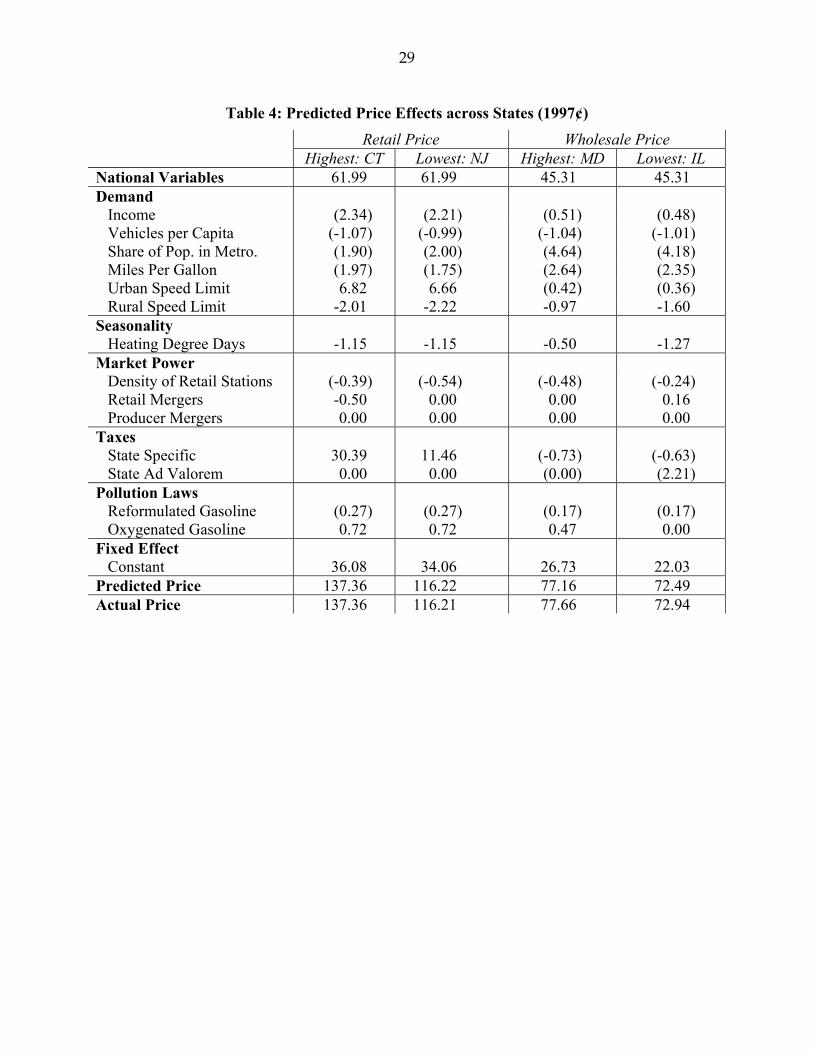
All states have some factors that raise prices and others that lower them. For specificity

in Table 4, we compare the price in the highest price state to that in the lowest price state.

(Comparisons by groups of states by deciles or quartiles produce similar patterns.)

Connecticut had the highest average predicted retail price, $1.37 per gallon, and New

Jersey had the lowest, $1.16. A few variables account for most of this 20¢ difference. Because

of a higher state specific tax, Connecticut consumers paid 18.93¢ (= 30.39¢ - 11.46¢) more than

did those in New Jersey. The urban and rural speed limit measures account for .4¢ of the

difference, and the fixed effects difference was 2¢.

Maryland had the highest average predicted wholesale price of 77¢ per gallon, and

Illinois had the lowest, 72¢. Maryland’s price tended to be higher than Illinois’s because of the

rural speed limit (0.6¢), heating-degree days (0.8¢), oxygenated gasoline (0.5¢), and the fixed

effects (4.7¢).

5. Conclusions

We believe that this study is the first cross-section, time-series analysis of gasoline

prices. Our first finding is that virtually the entire increase in national gasoline prices over the

last decade is due to a rise in the price of crude oil. Although politicians and others blamed

taxes, pollution laws, and market power, these factors have not trended over the decade and

hence did not substantially contribute to the rise in the real price of gasoline. Indeed, if anything,

these other factors slightly lowered the overall price. On average, the price of crude oil and

17

federal taxes accounted for 75 percent of the predicted average wholesale price and nearly 44

percent of the predicted retail price.

We find that retail gasoline prices vary across states primarily due to variations in taxes

and market power. States’ specific and ad valorem taxes are a major cause of the variation of

retail prices (though less so for wholesale prices). State specific taxes accounted for up to 22.2¢

per gallon of the retail price differential across states. Ad valorem taxes contributed up to

another 11.1¢ to the variation. Because mergers affect market power and efficiency, some raised

prices while others lowered them. Retail mergers resulted in up to 16.4¢ cross-state price

differentials, while producer mergers added another 9.8¢. The other factors that affect retail

prices are the urban speed limit measure, 7.3¢ differential, and the rural speed limit measure with

a 13.4¢ differential.

Mergers had the largest impact on wholesale price variation, while taxes had little effect.

Retail mergers contributed up to a 12.0¢ difference in wholesale prices across states, while

producer mergers added up to another 8.0¢.

Contrary to popular “wisdom,” anti-pollution regulations explain little of the trend or

variation in gasoline prices. We found a small effect on retail prices and no statistically

significant effect on wholesale prices from the federal law requiring reformulation of gasoline.

Even if we do not care about pollution, eliminating federal anti-pollution laws will have little

impact on prices. The California reformulated gasoline law raised the retail price in that state by

4¢, but had no effect on the wholesale price. The oxygenated gasoline laws explained up to a

0.9¢ variation across states during cold months.

How can a state lower its prices relative to other states? The simplest way to lower retail

gas prices in a state is to lower taxes. Consumers pay for half of the federal specific tax, three-

18

quarters of state ad valorem taxes, and all of state specific taxes. In principle, the most attractive

approach to lowering prices is to prevent mergers that increase market power but not those that

increase efficiency. These anticompetitive mergers have relatively large price effects. Of

course, whether governments can prevent only “bad” mergers remains an open question.

19

References

American Automobile Association, The Digest of Motor Laws 1990, 1995.

Barron, J. M., and J. R. Umbeck , “The Effects of Differential Contractual Arrangements: The

Case of Retail Gasoline Markets,” The Journal of Law and Economics, 27 (October 1984),

313-23.

Blass, Asher A. and Dennis W. Carlton, “The Choice of Organizational Form in Gasoline

Retailing and the Costs of Laws Limiting that Choice,” National Bureau of Economic

Research Working Paper, 1999.

Borenstein, Severin, “Selling Costs and Switching Costs: Explaining Retail Gasoline Margins,”

Rand Journal of Economics, 22 (Autumn 1991), 354-369.

Borenstein, Severin, and Andrea Shepard, Dynamic Pricing in Retail Gasoline Markets, Rand

Journal of Economics, 27 (Autumn 1996), 429-51.

Borenstein, Severin, and Andrea Shepard, “Sticky Prices, Inventories, and Market Power in

Wholesale Gasoline Markets,” Program on Workable Energy Regulation Working Paper,

August 2000.

Bureau of Labor Statistics, Consumer Price Index, 1998.

Council of State Governments, The Book of the States, 1990, 1992, 1994, 1996.

Dahl, Carol and Thomas Sterner, “Analyzing Gasoline Demand Elasticities: A Survey,” Energy

Economics, (July 1991), 203-10.

Energy Information Agency, Energy Information Sheets, July 1998a.

Energy Information Agency, Petroleum Marketing Monthly, 1993, 1995, 1997, 1998.

Energy Information Agency, Petroleum Supply Annual, Volume 2 1989-1998.

20

Gilbert, Richard and Justine Hastings, “Vertical Integration in Gasoline Supply: An Empirical

Test of Raising Rivals’ Costs,” Working Paper, (June 2001).

Marvel, Howard P., “The Economics of Information and Retail Gasoline Price Behavior: An

Empirical Analysis,” Journal of Political Economy, 84 (October 1976), 1033-60.

Marvel, Howard P., “Competition and Price levels in the Retail Gasoline Market,” Review of

Economics and Statistics, 6 (May 1978), 252-258.

National Oceanic and Atmospheric Administration, Local Climatological Data, 1989-1997.

National Petroleum News, National Petroleum News Factbook, 1988-1997.

National Petroleum Council, Petroleum Storage and Transportation National

Petroleum Council, Washington, D.C., 1989.

Securities Data, The Merger Yearbook, 1989-1998.

Scheffman, D. T. and Pablo T. Spiller, “Geographic Market Definition Under the U.S.

Department of Justice Merger Guidelines, Journal of Law and Economics, 30 (April 1987),

Shepard, Andrea, Price Discrimination and Retail Configuration, Journal of Political Economy,

99 (February 1991), 30-53.

Slade, Margaret E., “Conjectures, Firms Characteristics, and Market Structure: An Empirical

Analysis,” International Journal of Industrial Organization, 4 (December 1986), 347-370.

U.S. Bureau of the Census, State and Metropolitan Area Data Book, 1991.

U.S. Bureau of Census, Statistical Abstract of the United States, 1990-1997.

U.S. Department of Commerce, Survey of Current Business, August 1992, 1998.

U.S. Department of Transportation, Highway Statistics, 1988-1997.

U.S. Department of Transportation, Report to Congress, 1998.

21

U.S. Environmental Protection Agency, List of Reformulated Gasoline Program Areas, April

1999a.

U.S. Environmental Protection Agency, State Winter Oxygenated Fuel Programs, September

1999b.

22

Appendix

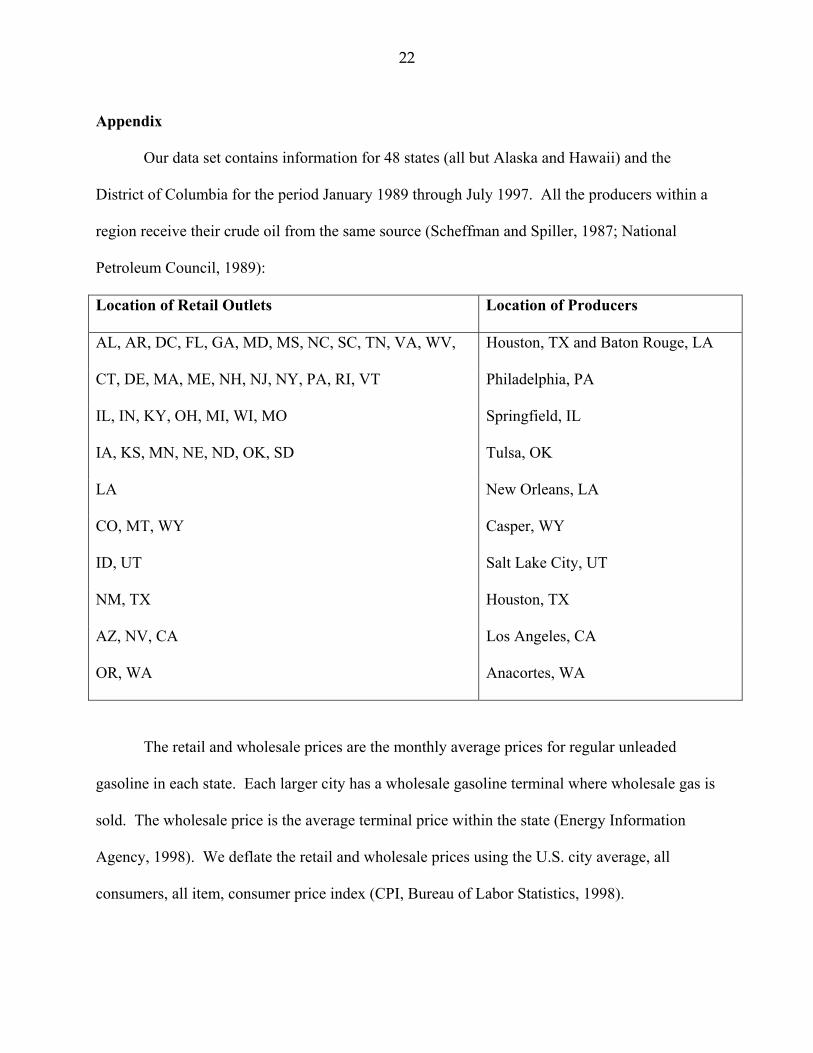
Our data set contains information for 48 states (all but Alaska and Hawaii) and the

District of Columbia for the period January 1989 through July 1997. All the producers within a

region receive their crude oil from the same source (Scheffman and Spiller, 1987; National

Petroleum Council, 1989):

Location of Retail Outlets Location of Producers

AL, AR, DC, FL, GA, MD, MS, NC, SC, TN, VA, WV, Houston, TX and Baton Rouge, LA

CT, DE, MA, ME, NH, NJ, NY, PA, RI, VT Philadelphia, PA

IL, IN, KY, OH, MI, WI, MO Springfield, IL

IA, KS, MN, NE, ND, OK, SD Tulsa, OK

LA New Orleans, LA

CO, MT, WY Casper, WY

ID, UT Salt Lake City, UT

NM, TX Houston, TX

AZ, NV, CA Los Angeles, CA

OR, WA Anacortes, WA

The retail and wholesale prices are the monthly average prices for regular unleaded

gasoline in each state. Each larger city has a wholesale gasoline terminal where wholesale gas is

sold. The wholesale price is the average terminal price within the state (Energy Information

Agency, 1998). We deflate the retail and wholesale prices using the U.S. city average, all

consumers, all item, consumer price index (CPI, Bureau of Labor Statistics, 1998).

23

The domestic price of crude oil is the first-purchase price (the price refiners pay) of crude

oil per barrel in Texas (Energy Information Agency, 1993, 1995, 1997). Because each barrel of

crude oil produces 44 gallons of petroleum product (Energy Information Agency, 1998), we

obtain the price per gallon by dividing the price per barrel of crude oil by 44.

We obtained the annual average income for each state and the monthly national income

from the U.S. Department of Commerce (1992, 1998). We interpolated each state’s real annual

per capita income using the national trend to obtain a monthly series.

The state population density is the percentage of each state’s population that resides in a

statistically defined metropolitan area (U.S. Bureau of Census, 1990-1997).

The number of annual registered (privately owned and publicly held) vehicles for each state was

obtained from the U.S. Department of Transportation (1988-1997). A monthly series of vehicles

was generated by linear interpolation. We then calculated obtained the per capita number of

vehicles by dividing by the monthly state population over the age of sixteen.

Our measure of the average automobile fuel efficiency for the vehicle fleet in a state was

calculated by dividing the total number of miles driven in each state by the total amount of

gasoline consumption (U.S. Department of Transportation, 1988-1997). The urban (rural) speed

limit for a state is the speed limit on urban (rural) interstates (American Automobile Association,

1990, 1995; U.S. Department of Transportation, 1998) multiplied by the percentage of interstate

miles driven on urban (rural) interstates for that state (U.S. Department of Transportation, 1988-

1997).

The federal specific gasoline tax, measured in cents per gallon, is from U.S. Department

of Transportation (1988-1997), and the state retail gasoline taxes are from U.S. Department of

Transportation (1988-1997). We used the CPI to deflate these specific taxes. The ad valorem

24

taxes, a percentage, for California, Georgia, Illinois, Indiana, Louisiana, Michigan, Mississippi,

and New York are from the Council of State Governments (1990, 1992, 1994, 1996). Other

states do not apply an ad valorem tax to the retail price of gasoline.

We calculate the percentage of retail outlets per square mile by dividing the number of

outlets that sell gasoline at the retail level (National Petroleum News, 1996, 1998) by each state’s

area (U.S. Bureau of the Census, 1991) and multiplied by 100.

The distance variable is the number of miles from the nearest refinery to the largest city

in each state. We use the heating degree-days for a representative city for each state.

The contractual arrangement variables between the retailers and wholesalers are the

national percentage of the 20 largest major branded retail gasoline stations that are operated

under a lease contract, are operated by a vertically integrated company or are open dealers

(National Petroleum News, 1988-1997). These variables vary over time, but not across

jurisdictions.

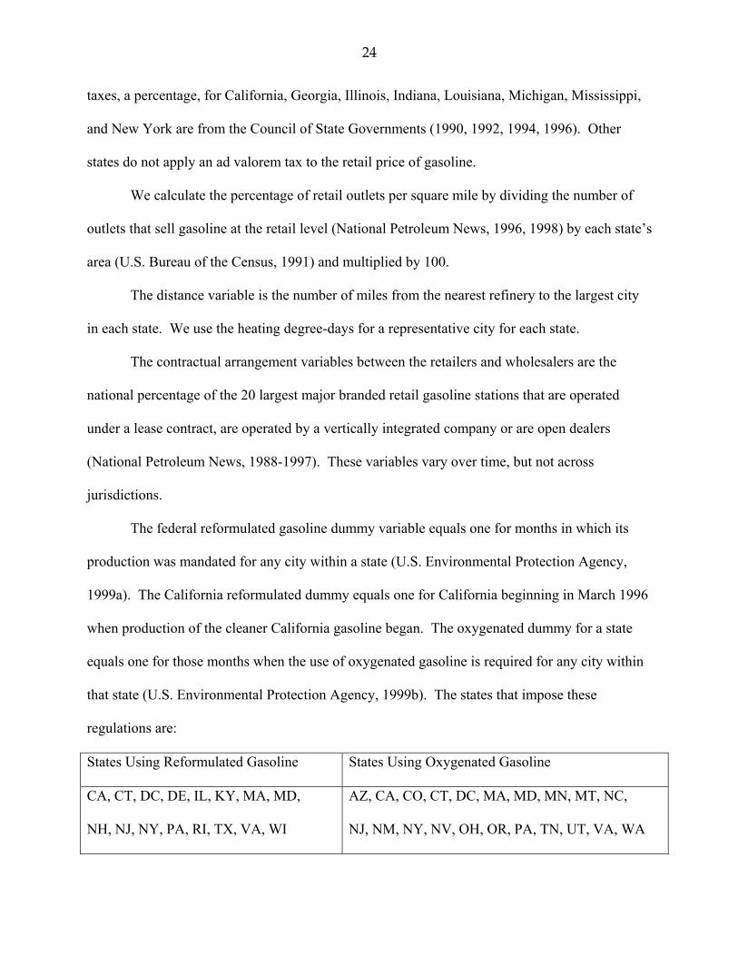
The federal reformulated gasoline dummy variable equals one for months in which its

production was mandated for any city within a state (U.S. Environmental Protection Agency,

1999a). The California reformulated dummy equals one for California beginning in March 1996

when production of the cleaner California gasoline began. The oxygenated dummy for a state

equals one for those months when the use of oxygenated gasoline is required for any city within

that state (U.S. Environmental Protection Agency, 1999b). The states that impose these

regulations are:

States Using Reformulated Gasoline States Using Oxygenated Gasoline

CA, CT, DC, DE, IL, KY, MA, MD,

NH, NJ, NY, PA, RI, TX, VA, WI

AZ, CA, CO, CT, DC, MA, MD, MN, MT, NC,

NJ, NM, NY, NV, OH, OR, PA, TN, UT, VA, WA

25

The Persian Gulf War dummy variable equals one during the period of fighting, January

1991 and June 1991. For each merger that affects wholesale or retail ownership, a states-specific

dummy is set equal to one from the effective date of a merger (Securities Data, 1989-1998).

26

Table 1: Means and Standard Deviations

Variable Mean Standard Deviation Prices Retail (¢ per gallon) 125.86 12.43 Wholesale (¢ per gallon) 74.88 12.74 Demand Disposable Family Income ($1000 per month) 1.83 0.31 Registered Vehicles per Capita 0.79 0.13 Share of Population in Metro. Area (%) 67.17 21.82 Average Miles Driven Per Gallon 16.41 1.31 Urban Speed Limit x Fraction on Urban Highways 28.81 12.23 Rural Speed Limit x Fraction on Rural Highways 32.35 15.20 Cost Crude Oil Price (¢ per gallon) 46.89 9.98 Persian Gulf War (0 – 1) 0.06 Seasonality Heating Degree Days (divided by 100) 3.58 3.79 Market Power Density of Retail Stations (total number of stations divided by square mile times 100)

16.36 32.66

Taxes Federal (¢ per gallon) 16.59 3.00 State Specific (¢ per gallon) 20.90 4.73 State Ad Valorem (%) 0.80 1.87 Pollution Laws Federal Reformulated Gasoline Law (0 – 1) 0.10 California Reformulated Gasoline Law (0-1) 0.003 Oxygenated Gasoline Law (0 – 1) 0.08 Vertical Relations Lease Operated (%) 16.92 6.88 Company Operated (%) 6.74 0.76

27

Table 2: Retail and Wholesale Reduced-Form Price Equations (1997¢)

Retail Wholesale Variable coefficient t-statistic Coefficient t-statistic Demand Income 0.91 1.23 0.23 0.31 Vehicles per Capita -1.34 -0.82 -1.42 -0.88 Share of Pop. In Metro. Area 0.02 0.52 0.05 1.26 Miles Per Gallon 0.11 0.84 0.15 1.18 Urban Speed Limit 0.15 3.39 0.01 0.27 Rural Speed Limit -0.21 -6.66 -0.07 -2.23 Cost Crude Oil Price 0.64 33.34 0.82 43.71 Crude Oil Price Lagged Once 0.15 5.00 0.05 1.60 Crude Oil Price Lagged Twice 0.21 11.03 0.13 6.77 Persian Gulf War 1.68 5.01 3.01 9.12 Seasonality Heating Degree Days -0.21 -4.78 -0.24 -5.65 Market Power Density of Retail Stations -0.01 -1.41 -0.02 -1.93 Taxes Federal 0.48 11.11 -0.54 -12.73 State Specific 0.97 23.79 -0.03 -0.76 State Ad Valorem 1.73 3.60 0.36 0.77 Pollution Laws Federal Reformulated Gasoline 0.81 2.91 0.50 1.80 CA Reformulated Gasoline 3.85 2.40 1.25 0.79 Oxygenated Gasoline 3.65 13.22 2.93 10.77 Vertical Relations Lease Operated 0.29 15.24 0.17 9.25 Company Operated -0.005 -0.05 0.06 0.69 R-Squared 0.89 0.90

28

Table 3: Average and Range Effects on Prices (1997¢)

Retail Price Wholesale Price Variable Mean Range Mean Range Demand Income (1.67) (1.12) (0.42) (0.28) Vehicles per Capita (-1.06) (0.91) (-1.12) (0.97) Share of Pop. in Metro. Area (1.34) (1.52) (3.36) (3.81) Miles Per Gallon (1.81) (0.55) (2.47) (0.75) Urban Speed Limit 4.32 7.31 (0.29) (0.49) Rural Speed Limit -6.79 13.35 -2.26 4.45 Cost Crude Oil Price 30.01 38.45 Crude Oil Price Lagged Once 7.05 (2.35) Crude Oil Price Lagged Twice 9.88 6.12 Persian Gulf War 0.10 0.18 Seasonality Heating Degree Days -0.75 0.93 -0.86 1.06 Months 2.12 3.89 Market Power Density of Retail Stations (-0.16) (2.20) (-0.33) (4.41) Retail Mergers 0.01 16.36 -0.11 11.99 Producer Mergers 0.15 9.79 0.13 7.92 Taxes Federal 7.96 -8.96 State Specific 20.27 22.20 (-0.63) (0.69) State Ad Valorem 1.39 11.12 (0.29) (2.31) Pollution Laws Federal Reformulated Gasoline 0.09 0.27 (0.05) (0.17) CA Reformulated Gasoline 0.01 0.53 (0.004) (0.17) Oxygenated Gasoline 0.41 0.90 0.33 0.73 Vertical Relations Lease Operated 4.91 2.88 Company Operated (-0.03) (0.40) Constant 41.23 27.24 Predicted Price 125.90 74.56 Actual Price 125.86 74.88

29

Table 4: Predicted Price Effects across States (1997¢) Retail Price Wholesale Price Highest: CT Lowest: NJ Highest: MD Lowest: IL National Variables 61.99 61.99 45.31 45.31 Demand Income (2.34) (2.21) (0.51) (0.48) Vehicles per Capita (-1.07) (-0.99) (-1.04) (-1.01) Share of Pop. in Metro. (1.90) (2.00) (4.64) (4.18) Miles Per Gallon (1.97) (1.75) (2.64) (2.35) Urban Speed Limit 6.82 6.66 (0.42) (0.36) Rural Speed Limit -2.01 -2.22 -0.97 -1.60 Seasonality Heating Degree Days -1.15 -1.15 -0.50 -1.27 Market Power Density of Retail Stations (-0.39) (-0.54) (-0.48) (-0.24) Retail Mergers -0.50 0.00 0.00 0.16 Producer Mergers 0.00 0.00 0.00 0.00 Taxes State Specific 30.39 11.46 (-0.73) (-0.63) State Ad Valorem 0.00 0.00 (0.00) (2.21) Pollution Laws Reformulated Gasoline (0.27) (0.27) (0.17) (0.17) Oxygenated Gasoline 0.72 0.72 0.47 0.00 Fixed Effect Constant 36.08 34.06 26.73 22.03 Predicted Price 137.36 116.22 77.16 72.49 Actual Price 137.36 116.21 77.66 72.94

30

Figure 1 Markups Over Time

1989 1990 1991 1992 1993 1994 1995 1996 19970

20

40

60

80

100

120

140

Retail (netof taxes)

Wholesale

Crude Oil

Prices (1997 ¢)

1989 1990 1991 1992 1993 1994 1995 1996 19970

20

40

60

Wholesale -Crude Oil

Retail -Wholesale

Price Differences (1997 ¢)

(a)

(b)

31

Figure 2 Determinants of Retail Prices

1989 1990 1991 1992 1993 1994 3/1995 1996 19970

20

40

60

80

100

120

140

160

180Price (1997¢)

All Other

Crude Oil

Cyclical

Predicted (line)Actual RetailPrices (points)

32

Figure 3 Determinants of Wholesale Prices

1989 1990 1991 1992 1993 1994 1995 1996 1997-20

0

20

40

60

80

100

120

Price (1997¢)

All Other

Crude Oil

Cyclical

Predicted (line)

Actual RetailPrices (points)