Embed Size (px)
Citation preview

TJ778.M41.G24
AN ANALYTICAL AND NUMERICATHE SECOND-ORDER EFFECTs OF I
ON THE PERFORMANCE OF TURB
by
Gerd Fritsch
GTh Report #2 10
GAS TURBINE LABORATORYMASSACHUSETTS INSTITUTE OF TECHNOLOGYCAMBRIDGE, MASSACHUSETTS
i 01

AN ANALYTICAL AND NUMERICAL STUDY OFTHE SECOND-ORDER EFFECTS OF UNSTEADINESS
ON THE PERFORMANCE OF TURBOMACHINES
by
Gerd Fritsch
GTL Report #210 June 1992
This research was supported by the Air Force Office of Scientific Researchgrant AFOSR-90-0035, supervised by Major Daniel Fant as the TechnicalMonitor.

An Analytical and Numerical Study of the Second-Order
Effects of Unsteadiness on the Performance of
Turb omachines
by
Gerd Fritsch
A linear approach in two dimensions is used to investigate the second-order effects
of unsteadiness on the efficiency of turbomachines. The three main themes are the iden-
tification of physical nature and location of unsteady loss mechanisms, the magnitude
of the associated losses and their effect on the time-mean efficiency, and the assessmentof the modeling accuracy of numerical simulations with respect to unsteady loss.
A mathematically rigorous link is established between linear waves in a compressible,two-dimensional flow and the efficiency drop associated with their dissipation. The anal-
ysis is applied to the mixing loss at the interface in a steady simulation of rotor/stator
interaction in a turbine and to the study of unsteady loss mechanisms.
Two unsteady loss mechanisms are considered. Unsteady Circulation Loss, i.e. the
transfer of mean-flow energy to kinetic energy associated with vorticity shed at the trail-
ing edge in response to an unsteady circulation, was first considered by Keller (1935)and later by Kemp and Sears (1955). Keller's original work is extended to compress-ible, homentropic flows. The use of simulations to obtain circulation amplitudes avoids
the limitations of thin-airfoil theory and yields a loss measure realistic for modern tur-bomachines. For the Unsteady Viscous Loss mechanism, i.e. the dissipation inducedby pressure waves in unsteady boundary layers, the high-reduced-frequency limit and anear-wall approximation are used to obtain the local velocity distribution in the laminarStokes sublayer and the corresponding time-mean dissipation. The input to the model
are the unsteady pressure gradients along a blade surface obtained from an unsteadysimulation. A numerical study of the errors due to modeling approximation is included.
Both sources of loss are small but not negligible. It is found that numerical smooth-
ing shifts the principal locus of unsteady dissipation from boundary layers to thefreestream, reducing the magnitude of the loss models input and the predicted loss.
2

Acknowledgments
It all started a little more than four years ago, when I concluded that it wasn't
quite the time yet to settle down in southern Germany. Now, with almost four years of
graduate study behind me, I have only one last page to go ...
Looking back, I can call these years at MIT an important and rewarding experience
both in academic and personal terms. It was an experience that I would not want to
have missed, although there have been innumerable times when I wished I had never
asked for the application forms.
First, I would like to express my gratitude to my advisor, Prof. Michael B. Giles, for
his support, advice, and encouragement throughout this project. He was an excellent
teacher as well, and always had an open ear for my ideas and problems. I would like
to thank Prof. Edward M. Greitzer for his constructive criticism and encouragement.
Thanks also to Prof. Mark Drela for his helpful comments, and to the readers, Profs.
Marten T. Landahl and Alan H. Epstein, for their suggestions.
Thanks in no small measure is due to my fellow students in the CFD-Lab; their
company and support have helped this project more than they may realize. Special
thanks goes to Guppy, my climbing partner and friend, who constantly reminded me
that there is life outside MIT. Countless are the summer days, when he tempted me
with outdoor endeavors; needless to say that he met little resistance.
Special thanks also goes to Patrick and Harold for their friendship. Not only have
they tolerated my little-refined social skills (not without the appropriate comments)
and provided for many an interesting discussion, they have also been superb company
in such diverse places as the Yucatan Peninsula of Mexico, Yosemite National Park in
California, Acadia National Park in Maine, the many rocks of the East Coast, and, all
too often, MIT.
Finally, I would like to thank Denise, my friend and fiancee. Her friendship, love,
support, and fighting spirit contributed greatly to this project. With my departure, she
will finally be able to cut her last physical link to MIT, three years after she graduated.
Despite accompanying me through the second half of my studies at MIT, she has decided
to pursue a doctoral study of her own. I hope that I can be as much of a backing to
Denise during her upcoming Promotion in Germany as she was to me.
This research was supported by the Air Force Office of Scientific Research grant
AFOSR-90-0035, supervised by Major Daniel Fant as the Technical Monitor.
3

Contents
Abstract
Acknowledgments
Nomenclature
1 Introduction
1.1 M otivation . . . . . . . . . . . . . . . . . . . . . . . . . . . . . . . . .
1.2 Unsteadiness and Loss - Historical Perspective . . . . . . . . . . . . .
1.3 Thesis Outline . . . . . . . . . . . . . . . . . . . . . . . . . . . . . . .
2 Unsteadiness and Loss
2.1 Unsteady Modes . . . . . . . . . . . . . . . . . . . .
2.2 Dissipation and Rectification . . . . . . . . . . . . .
2.2.1 Conditions and Mechanism for Rectification .
2.2.2 Wave Transmission and Reflection . . . . . .
2.3 Loss Due to Dissipation of Waves . . . . . . . . . . .
2.3.1 Flux-Averaging . . . . . . . . . . . . . . . . .
2.3.2 Entropy Rise . . . . . . . . . . . . . . . . . .
2.3.3 Interpretation of the Entropy Rise . . . . . .
2.4 A Note on Numerical Smoothing . . . . . . . . . . .
2.5 Efficiency Considerations . . . . . . . . . . . . . . .
4
2
3
12
16
17
18
21
23
. . . . . . . . . . . 24
. . . . . . . . . . . 27
. . . . . . . . . . . 28
. . . . . . . . . . . 29
. . . . . . . . . . . 31
. . . . . . . . . . . 32
. . . . . . . . . . . 37
. . . . . . . . . . . 40
. . . . . . . . . . . 43
. . . . . . . . . . . 45

2.6
2.7
2.8
2.5.1 Total Pressure Loss . . . . . . . . . . . . . . . . . . . . . . . . .
2.5.2 Linearized Efficiency . . . . . . . . . . . . . . . . . . . . . . . . .
Numerical Check and Accuracy . . . . . . . . . . . . . . . . . . . . . . .
Mixing Loss at Steady Interfaces in CFD . . . . . . . . . . . . . . . . .
Summary - Unsteadiness and Loss . . . . . . . . . . . . . . . . . . . .
3 Unsteady Circulation Loss
3.1 Analytical Theory . . . . . . . . . . . . . . . . . . . . . . . .
3.1.1 Single Airfoil . . . . . . . . . . . . . . . . . . . . . . .
3.1.2 Cascade . . . . . . . . . . . . . . . . . . . . . . . . . .
3.1.3 Cross-Induced Kinetic Energies . . . . . . . . . . . . .
3.2 Results - Unsteady Circulation Loss . . . . . . . . . . . . .
3.2.1 Single-Stage, Large-Scale Turbine No. 2 at Cambridge
3.2.2 Large Scale Rotating Rig (LSRR) at UTRC . . . . . .
3.2.3 Cold Air Turbine Stage at the DFVLR . . . . . . . . .
3.2.4 ACE Turbine Stage . . . . . . . . . . . . . . . . . . .
3.2.5 NASA Stage 67 Compressor . . . . . . . . . . . . . . .
3.3 Summary - Unsteady Circulation Loss
4 Unsteady Viscous Loss
4.1 Analytical Approach . . . . . . . . . .
4.1.1 Governing Equations . . . . . .
4.1.2 Linearization . . . . . . . . . .
4.1.3 Nondimensionalization . . . . .
4.1.4 High-Reduced-Frequency Limit
5
45
45
50
53
61
62
. . . . . . 64
. . . . . . 64
. . . . . . 68
. . . . . . 71
. . . . . . 76
. . . . . . 76
. . . . . . 78
. . . . . . 79
. . . . . . 81
. . . . . . 83
85
87
92
93
93
94
95

4.1.5 High-Frequency Limit of the Momentum Equation . . . . . . . . 97
4.1.6 Free-Stream and Near-Wall Approximation . . . . . . . . . . . . 97
4.1.7 Streamwise Velocities in the High-Frequency Limit . . . . . . . . 98
4.1.8 Unsteady Dissipation . . . . . . . . . . . . . . . . . . . . . . . . 100
4.1.9 Unsteady Viscous Loss and Efficiency . . . . . . . . . . . . . . . 102
4.2 Analytical Evaluation of Modeling Errors . . . . . . . . . . . . . . . . . 104
4.2.1 Convective Terms in the Momentum Equation - Global . . . 105
4.2.2 Convective Terms in the Momentum Equation - Near the Wall 106
4.3 Numerical Evaluation of Modeling Errors . . . . . . . . . . . . . . . . . 107
4.3.1 Model Problem . . . . . . . . . . . . . . . . . . . . . . . . . . . . 107
4.3.2 Code Verification in Laminar Flow . . . . . . . . . . . . . . . . . 111
4.3.3 Errors in the Integrated Dissipation for Laminar Flow . . . . . . 113
4.3.4 Code Verification in Turbulent Flow . . . . . . . . . . . . . . . . 115
4.3.5 Errors in the Integrated Dissipation for Turbulent Flow . . . . . 118
4.4 Unsteady Loss in the ACE Turbine Stage . . . . . . . . . . . . . . . . . 122
4.4.1 Application of the Unsteady Viscous Loss Model . . . . . . . . . 124
4.4.2 Efficiencies in the Numerical Simulation . . . . . . . . . . . . . . 126
4.4.3 The Role of Numerical Smoothing . . . . . . . . . . . . . . . . . 128
4.4.4 Entropy Rise in the Simulation . . . . . . . . . . . . . . . . . . . 134
4.5 Summary - Unsteady Viscous Loss . . . . . . . . . . . . . . . . . . . . 138
5 Concluding Remarks 140
5.1 Sum m ary . . . . . . . . . . . . . . . . . . . . . . . . . . . . . . . . . . . 140
5.1.1 Chapter 2 - Unsteadiness and Loss . . . . . . . . . . . . . . . . 140
5.1.2 Chapters 3 and 4 - Unsteady Loss Mechanisms . . . . . . . . . 142
6

5.2 Future
5.2.1
5.2.2
Bibliography
Work Reconimendations . . . . . . . . . . . . . . . . . . . . . .
Chapter 2 - Unsteadiness and Loss . . . . . . . . . . . . . . .
Chapter 4 - Unsteady Viscous Loss . . . . . . . . . . . . . . .
Appendices
A Derivatives of the Axial Flux Vector
B Derivatives of the Axial Entropy Flux
C Orthogonalities of Trigonometric Functions
D Separation Properties for Non-Evanescent Pressure Waves
E Separation Properties for Evanescent Pressure Waves
F Single Evanescent Pressure Waves
G Left Eigenvectors of the Linearized Euler Equations
H Scaling Arguments in the Near-Wall Approximation
I Length and Time Scales in Turbulent Flow
J Attenuation of Pressure Waves at Boundaries
7
145
145
146
147
153
153
154
155
156
158
162
163
164
166
167

List of Figures
2.1 Rectification of unsteady waves . . . . . . . . . . . . . . . . . . . . . . .
2.2 Control volume for the asymptotic analysis . . . . . . . . . . . . . . . .
2.3 Compound phase and amplitude as a function of the axial position . . .
2.4 Control volume - revisited for propagating pressure waves . . . . . . .
2.5 Control volume - revisited for evanescent pressure waves . . . . . . . .
2.6 ht - s diagram for an ideal gas . . . . . . . . . . . . . . . . . . . . . . . .
2.7 Total pressure loss and isentropic efficiency drop for a turbine . . . . . .
2.8 Total pressure loss and polytropic efficiency drop for a turbine . . . . .
2.9 Total pressure loss and isentropic efficiency drop for a compressor . . . .
2.10 Accuracy of the second-order entropy rise (Q = 0) . . . . . . . . . . . .
2.11 Accuracy of the second-order entropy rise (n = 4) . . . . . . . . . . . .
2.12 Static pressure contours in an unsteady simulation of the ACE turbine
stage for (t/T ) = 0.7 . . . . . . . . . . . . . . . . . . . . . . . . . . . . .
2.13 Static pressure contours in a steady simulation of the ACE turbine stage
2.14 Entropy rise in the simulations of the ACE turbine stage . . . . . . . . .
2.15 Stage geometry and computational grid of the ACE turbine stage for
(t/T ) = 0.7 . . . . . . . . . . . . . . . . . . . . . . . . . . . . . . . . . .
8
28
33
36
42
43
46
48
49
50
51
52
54
55
56
57

2.16 Decomposition of the entropy rise into the wave types and wavenumbers
(fundamental wavenumber kyl corresponds to the stator pitch) . . . . . 58
3.1 An isolated airfoil with an unsteady lift and circulation . . . . . . . . . 64
3.2 A cascade with an unsteady lift and circulation . . . . . . . . . . . . . . 68
3.3 Relative magnitude of the spatial harmonics in the shed vorticity wake
(first harmonic corresponds to the pitch of the upstream blade row) . . 74
3.4 Relative amount of kinetic energy in higher spatial harmonics . . . . . . 75
4.1 Steady boundary layer subject to a discontinuous freestream velocity . . 87
4.2 Unsteady boundary layer on an oscillating wall . . . . . . . . . . . . . . 88
4.3 Unsteady boundary layer on a blade surface . . . . . . . . . . . . . . . . 89
4.4 Unsteady boundary layer on a blade - simulation of the ACE turbine
stage at (t/T) = 0.9 . . . . . . . . . . . . . . . . . . . . . . . . . . . . . 90
4.5 Unsteady streamwise velocity distribution as a function of the wall distance100
4.6 Dissipation rate for the 'exact' solution and the high-frequency limit . . 102
4.7 ht - s diagram for an ideal gas - revisited and magnified . . . . . . . . 103
4.8 Model problem for the numerical evaluation of modeling errors . . . . . 108
4.9 Comparison to Lighthill's analytic solution in laminar flow . . . . . . . .
4.10 Comparison between 'exact' numerical solution and high-frequency limit
4.11 High-frequency-limit model and 'exact' laminar model dissipation. . .
4.12 Comparison to Cousteix's experiment - unsteady streamwise velocity
9
112
113
114
116

4.13 Comparison to Cousteix's experiment - unsteady velocity phase . . .
4.14 High-frequency-limit model and 'exact' turbulent model dissipation -
downstream propagating pressure waves . . . . . . . . . . . . . . . . . .
4.15 High-frequency-limit model and 'exact' turbulent model dissipation -
upstream propagating pressure waves . . . . . . . . . . . . . . . . . . . .
4.16 Unsteady streamwise velocity distribution in a turbulent mean flow -
upstream propagating pressure waves . . . . . . . . . . . . . . . . . . .
4.17 Unsteady streamwise velocity distribution near the wall in a turbulent
mean flow - upstream propagating pressure waves . . . . . . . . . . . .
4.18 Entropy rise per unit surface length on the ACE rotor . . . . . . . . . .
4.19 Attenuation of an acoustic wave in an unsteady boundary layer . . . . .
4.20 Average entropy in the rotor passage H-grid (the freestream) . . . . . .
117
118
119
120
121
124
130
134
4.21 Average entropy in the 0-grid (boundary layers) around the rotor blades 136
4.22 Time-mean rotor surface entropy . . . . . . . . . . . . . . . . . . . . . . 137
E.1 Eigenvectors for evanescent pressure waves in the complex plane . . . . 159
J.1 Normal velocity vectors in viscous and inviscid flow . . . . . . . . . . . . 168
10

List of Tables
Contributions to the entropy rise at the interface - by wave type . . . 59
Contributions to the entropy rise at the interface - by wavenumber . . 60
Input parameters for the simulation of the Cambridge No.2 turbine . . 76
Unsteadiness parameters and results for the Cambridge No.2 turbine . 77
Input parameters for the LSRR simulation . . . . . . . . . . . . . . . . . 78
Unsteadiness parameters and results for the LSRR . . . . . . . . . . . . 79
Input parameters for the DFVLR turbine simulation . . . . . . . . . . . 80
Unsteadiness parameters and results for the DFVLR turbine . . . . . . 80
Input parameters for the ACE turbine stage simulation . . . . . . . . . 81
Results for the ACE turbine stage . . . . . . . . . . . . . . . . . . . . . 82
Input parameters for the NASA stage 67 simulations . . . . . . . . . . . 83
Results for the NASA stage 67 simulations . . . . . . . . . . . . . . . . . 84
4.1 Input parameters for the ACE turbine stage simulation . . . . . . . . .
Modal contributions to the Unsteady Viscous Loss of the ACE rotor .
Isentropic efficiencies for the steady and the unsteady ACE simulation
123
125
127
11
2.1
2.2
3.1
3.2
3.3
3.4
3.5
3.6
3.7
3.8
3.9
3.10
4.2
4.3

Nomenclature
Latin Symbols
abCP
eet
eght
k
I
npn
PqrS
s9
tU
U,V
z
y
z
12
speed of soundreal amplitudeblade chord or blade axial chordblade axial chordspecific heat at constant pressureEuler's constanttotal specific energy of a fluid, et = ht - (pIp)
jth unit vector, ej = [65 ij, 62 3j, 64jtotal specific enthalpy of a fluid
wave number,reduced frequencies, defined in equation (3.5) or (4.6)
length scaletemporal and spatial mean of the secondary kinetic energy
polytropic exponentcoordinate normal to a blade surface
pressureheatkinetic energy ratio, defined in equation (3.41)
entropy,blade surface coordinatenondimensional time-mean mass-average entropy, defined in (2.36)time
velocity in the direction of the coordinate x or s
wall friction velocity, defined in (4.89)
velocity in the direction of the coordinate y or n
eigenvectoraxial coordinateconvected coordinate, in the mean flow direction
circumferential coordinateconvected coordinate, normal to the mean flow
coordinate in the direction of wave propagation
matrices in the Euler equations in primitive form, defined in (2.5)
complex amplitudes of the potential functions (3.8) and (3.24)
matrix to calculate the second-order entropy rise in (2.36)acoustic energy density, defined in equation (2.41)flux vectors in the Euler equations, defined in equation (2.2)
matrix to calculate second-order mean flow changes in (2.30)high-reduced-frequency limit
A, BA, BDEF, GHHFL

I acoustic intensity
N acoustic energy flux defined in equation (2.41)
M Mach number
P pitch
rotated pitch (in a convected coordinate system), P = P cos a
P* pitch of the neighboring blade row in a single stage
Pr Prandtl number
R square root of the discriminant defined in (2.16),specific gas constant
R acoustical impedance
Re Reynolds number
Re, Reynolds number defined with the local coordinate s
Re 9 Reynolds number defined with the momentum thickness 0
S entropy flux in subsection 2.3.2, S = pus
T period,characteristic time,temperature
Tf forcing time scale (blade passing period or an integer fraction thereof)
U state vector defined in equation (2.2) or (2.5)
Ue freestream convection velocity
VR rotor speed
Greek Symbols
a angle between the blade wake and the axial direction
)3 inter-blade phase angle,amplitude attenuation factor
18 inter-blade phase angle in a convected coordinate system
-y ratio of specific heat for an ideal gas,vortex sheet strength
6 boundary layer thickness
bf unsteady boundary layer thickness
61 laminar sublayer layer thickness in turbulent flow
b, viscous length scaleP* displacement thickness6zi Kronecker delta function, defined in appendix C
E small (perturbation) parameter
E2 , e4 second-difference and fourth-difference smoothing coefficients
efficiency
0 angle between the wave propagation direction and the surface normal
K thermal conductivity
A a reduced frequency defined in equation (3.22)
Af wavelength of a disturbance driving the unsteady boundary layer
Y dynamic viscosity
13

V kinematic viscosity
7rt total pressure ratio
p densitya- normal stress7' shear stress
rt total temperature ratio
4> potential function<p phase anglew angular frequencyWf forcing frequency, blade passing frequency
I circulationA difference,
small perturbation,grid spacing
<I> dissipation function, first defined in equation (4.14)
fl reduced frequency defined in equation (2.11),control volume, volume of integration
dn control volume boundary
Others
R( ), 9() real and imaginary part of a complex quantity
V gradient operator
Subscripts
e at the boundary layer edge
i integrated,incoming
in at the inflow boundaryinv inviscid1 leftM mth spatial/temporal harmonic
n nth temporal harmonic,in/normal to the direction of n
p in primitive form,polytropic
o fluid state after the dissipation of unsteady waves
out at the outflow boundary
r right,reflected,arbitrary reference state
14

isentropic,in/normal to the direction of s,based on the local value of the coordinate s
total/stagnation quantity,turbulentvelocity in the direction of the coordinate x or s
velocity in the direction of the coordinate y or n
viscousat the wallin the direction of the coordinate x,in the direction of the coordinate y
S
t
U
V
Visw
y
CDEHFLRS
01
2
3
4
0
00
Superscripts
T
zeroth-order, mean statefirst-order, first-order perturbation,entropy wave,fluid state before compressionsecond-order, second-order perturbation,vorticity wave,fluid state after compression
pressure wave propagating or decaying downstream,fluid state before expansion
pressure wave propagating or decaying upstream,fluid state after expansion
based on the momentum thickness
at infiuty
transposequantity in a convected coordinate system
unsteady quantitycomplex amplitude
temporal mean, temporal and spatial meanvector quantity
15
compressiondesignexpansionhigh-reduced-frequency limitrotorstator

Chapter 1
Introduction
Flow fields in turbomachinery are inherently unsteady, with a multitude of sources con-
tributing. The incoming flow itself can be nonuniform resulting in an unsteady inflow to
the rotor frame of reference. The relative motion of neighboring blade rows, in conjunc-
tion with the spatially nonuniform pressure fields locked to loaded blades, leads to an
unsteady pressure distribution in both through so-called potential interaction. A blade
row may also move through and interact with shock wave systems. Stator wakes con-
vected with the mean flow cause unsteadiness in the rotor frame of reference. Similarly,
secondary flow effects like horse shoe vortices, passage vortices, and tip clearance vor-
tices contribute to flow unsteadiness. The viscous flow past a blunt turbine trailing edge
results in vortex shedding; trailing-edge vortex shedding has also been found in com-
pressors operating in the transonic or supersonic regime. Finally, there is unsteadiness
induced by the motion of the blades themselves, i.e. blade flutter.
Very successful turbomachines have been developed in the past by compensating for
the lack of basic knowledge about unsteady effects or for their neglect with extensive
empirical correlations. The past two decades have seen a strong increase in the experi-
mental and computational effort devoted to unsteady flows in turbomachinery. Partly,
this increase was driven by a tremendous rise in the computing power and memory
available and by new or improved experimental facilities and techniques. Partly, it was
fueled by continuing demands to improve upon existing designs and design methodolo-
gies. To increase engine efficiencies and stability margins, to extent engine life-times, to
reduce weight and size, and to cut development cost and time, it is imperative to study
and understand unsteady flow phenomena. With turbomachinery efficiencies typically
around 90%, there is room left for improvement but one needs to look at all sources of
loss, including those considered too small or too difficult to treat before.
16
1.1 Motivation
Besides the general recognition of the importance of unsteady effects in turbomachinery,
several specific factors motivated this thesis.
First among them is the continuing prevalence of steady tools for routine design
purposes in industry. The standard aerodynamic design tools for turbomachinery are
steady codes, both inviscid and viscous, and steady cascade experiments. Designing
a single stage or blade row with steady-state tools amounts to placing the stator and
rotor row infinitely far apart thus eliminating the effects of blade row interaction. Un-
steadiness, however, contributes additional loss with non-zero time-meant First, most
of the energy associated with the unsteady part of the flow field is not recovered; it will
eventually be dissipated. Second, the interaction of unsteadiness with boundary layers
and shock structures can trigger additional loss. In a steady viscous simulation, the
effect of unsteadiness on the efficiency is not captured. An unsteady, nonlinear simu-
lation is still prohibitively expensive for routine design purposes and will likely remain
so in the foreseeable future, particularly for multistage turbomachinery. Testing of a
stage or a whole turbine under unsteady operating conditions will remain impractical
for routine design purposes. Therefore, the error in the predicted efficiency stemming
from the neglect of unsteady effects needs to be assessed.
Recently, linear perturbation methods have received increased attention as alterna-
tives to fully nonlinear, unsteady simulations. In linear CFD-codes, a nonlinear steady
state is found and the unsteady flow field is superimposed as a small perturbation.
Second-order terms, i.e. terms quadratic in unsteady quantities, are neglected since the
perturbations are assumed to be small. Linear perturbation codes have been found to
give accurate results up to a surprisingly high level of unsteadiness [1, 2] and will be
more widely used in the future. Linear codes, like steady codes, cannot capture un-
steady loss. The time-mean of the first-order unsteady dissipation is zero; only terms
second-order in unsteady quantities have a non-zero time-mean.
'This is not meant to imply that an increased spacing increases the efficiency.
See sections 1.2 and 2.7 for a further discussion of this point.
17

Most recently, CFD-codes have been developed which account for the second-order
effect of unsteadiness on the time-mean flow. Work in this direction has been pursued
by Adamczyk [3] and Giles [4]. In this context, the thesis research was intented to
underscore, or not, the need to include these effects.
Fully nonlinear, unsteady, viscous CFD-codes are another tool to evaluate unsteady
loss. However, the weakest point of any numerical simulation, steady or unsteady,
remains the accurate prediction of heat loads and losses due to the unavailability of
adequate turbulence and transition models. Thus, there is a need to examine the mod-
eling accuracy of numerical simulations with respect to unsteady flow phenomena and
unsteady losses. Throughout this thesis research, the CFD-code UNSFLO by Giles
[5, 6, 7], and the visualization package VISUAL2 by Giles and Haimes [8] were used.
The turbomachinery community is moving towards the consensus that increased
losses under unsteady operating conditions are primarily due to strongly nonlinear ef-
fects like the alteration of the boundary layer characteristics through their effect on
transition [9], the variation of secondary flow generation in downstream blade passages,
and their effect on separation or reattachment. Those effects are beyond the realm
of the linear/quadratic approach taken in this thesis. Nevertheless, the magnitude of
effects that can be treated in a linear framework, remains to be determined.
1.2 Unsteadiness and Loss - Historical Perspective
Theoretical and Experimental Work
Unsteadiness affects the efficiency of turbomachinery in a variety of ways. What follows
is a necessarily incomplete list of subjects of past investigations.
One of the earliest investigations was done by Keller [10] in 1935, who considered
the transfer of mean-flow energy to the unsteady flow field through shedding of vorticity
in an incompressible flow. The vorticity is shed off the blade trailing edges in response
18

to circulation variations, and its kinetic energy cannot be recovered. Keller estimated
the circulation amplitudes and concluded that the rate of energy transfer is equivalent
to between 0.4% and 1% of the power delivered or consumed by the rotor. In 1955,
Kemp and Sears [11] applied thin-airfoil theory developed earlier [12, 13, 14], and used
in the approximate analysis of interference between blade rows [15], to calculate the
circulation variations, the shed vorticity, and the associated kinetic energy. They ar-
rived at the conclusion that the rate of energy transfer is, generally, much less than
estimated by Keller. In 1973, Hawthorne [16], who used a lifting-line approach, found
rates of energy transfer which are in line with those of Keller[10].
In 1970, Kerrebrock and Mikolajczak [17] advanced a wake transport model to ex-
plain experimentally observed stagnation temperature and pressure non-uniformities in
the stator exit plane of a compressor stage and their effect on the performance. In
1984, Ng and Epstein [18] measured large total temperature and pressure fluctuations
at three to four the times blade passing frequency in the rotor core flow of a compressor
stage. They proposed a moving shock model coupled to shed wake vorticity to explain
their origin and deduced the magnitude of the associated loss. The entropy rise due to a
moving shock was found to lead to a 0.15% drop in the efficiency while the mixing-out of
fluctuations led to a loss on the order of the wake loss. Additional losses were expected
from the interaction of the shed vorticity with downstream shock structures. Experi-
mental evidence for moving shocks in a compressor rotor has subsequently been found by
Strazisar [19]; Hathaway et el. [20] found vortex shedding in a axial-flow fan. Owen [21]
observed vortex shedding off a transonic compressor rotor in numerical simulations.
More than one source of unsteadiness affects the compressor performance upon vari-
ation of the blade row gaps; those include wake transport, potential interaction, and
wake mixing, among others. In 1970, Smith [22] reported an efficiency increase of 1% for
reduced gaps in an multistage compressor. Later, Mikolajczak [23] confirmed their find-
ings, while experiments by Hetherington and Moritz [24] contradicted them; the above
experiments suggest that choosing an aerodynamically optimal gap is not an easy task.
19

The first studies on the influence of unsteadiness on the profile loss and the effi-
ciency in attached flows appeared in the late sixties and early seventies [25, 26, 27].
Obremski and Fejer [28], as well as Walker [29], observed early transition in unsteady
flow, leading to a greater length of the blade surface being covered by turbulent flow.
Pfeil et al. [30, 31] observed unsteady transition on a flat plate subject to periodic
wake-type disturbances. The same transition mechanism was found in an axial-flow
compressor by Evans [32], and in an axial-flow turbine by Dring et al. [33]. Hodson [9]
investigated the effect of unsteady transition on a cascade and found an increase of
50% in the rotor profile loss for unsteady inflow; subsequently he proposed an unsteady
transition model [34]. Shock-wave/boundary layer interaction can lead to separation,
as observed by Doorly and Oldfield [35], for example.
Numerical Developments
The progress in the numerical simulation of unsteady flow over the past two decades has
been impressive. The range of methods includes linear potential [36, 37] and linear Euler
methods [1, 2, 38], as well as nonlinear codes solving the Euler [5, 6, 39, 40, 41, 42, 43] or
the Navier-Stokes equations [7, 44]. In linear (perturbation) methods, the steady flow is
a solution to the nonlinear potential equation or to the nonlinear Euler equations, and
the unsteady flow field is superimposed as a small perturbation. The appeal of linear
methods lies in the savings in CPU-time they offer over a fully nonlinear formulation.
In response to the impracticality of multistage, unsteady, viscous simulations, Adam-
czyk [3] formulated a system of equations to account for the time-mean effect of the de-
terinnistic periodic unsteadiness on the mean flow through second-order terms similar
to Reynolds stresses. In a research project related to this thesis, Giles [4] developed an
asymptotic approach to unsteady flow in multistage turbomachinery. The asymptotic
parameter is the level of unsteadiness in a flow described by the Euler equations. The
approach leads to separate equations for the mean flow, the first-order perturbations,
and the time-mean of the second-order perturbations. These can be solved more effi-
ciently than the full nonlinear equations, in particular for multistage turbomachinery.
20

A number of comparisons have been conducted between experiments and simula-
tions. Those were focusing, for example, on wake/stator interaction [5, 9, 42, 45], on
the redistribution of inlet temperature profiles in a turbine stage [46, 47, 48, 49], on
heat transfer in a turbine stage [50, 51, 52], or on the efficiency [53]. The weakest point
of any numerical simulation remains, as was noted earlier, the exact prediction of heat
loads and losses.
1.3 Thesis Outline
The first component of this thesis, chapter 2, focuses on the relation between unsteadi-
ness and loss in two dimensions. The unsteady waves that are solutions to the linearized
Euler equations are entropy and vorticity waves, convected with the mean flow, and pres-
sure waves of propagating or evanescent nature. Concluding that most of the energy
associated with the unsteadiness cannot be recovered, an asymptotic analysis in sec-
tion 2.3 yields the second-order mean flow change and entropy rise resulting from the
dissipation of an arbitrary combination of unsteady waves in a uniform mean flow. For
the use in subsequent chapters, section 2.5 links the entropy rise to a total pressure
loss and to a change in performance through a linearization of the isentropic efficiency.
The result of the analysis is used in section 2.6 to evaluate the accuracy of the linear
approach, and in section 2.7 to analyze mixing loss at the stator/rotor interface of a
steady simulation.
The second component of this thesis focuses on the nature and the location of
unsteady loss mechanisms and the magnitude of the associated losses. Two aspects are
covered, termed Unsteady Circulation Loss and Unsteady Viscous Loss, respectively.
Chapter 3 revisits the Unsteady Circulation Loss first treated by Keller [10] in 1935
and later by Kemp and Sears [11] in 1956. Keller estimated the unsteady circulation
amplitude to arrive at the kinetic energy in the unsteady flow field induced by the shed
vorticity. Sears and Kemp used thin-airfoil theory to obtain the unsteady circulation
amplitude. This approach, while enabling them to calculate the circulation amplitude,
21

limited them to incompressible flow and blades of zero thickness and camber with the
mean flow nearly in the blade direction, i.e. lightly loaded blades. Thus, the airfoils
are more representative of compressor blades than turbine blades. In this thesis, the
circulation amplitudes are obtained from numerical simulations, which allows one to
obtain amplitudes for arbitrary blade and stage geometries, steady lift distributions,
and Mach numbers. Kelvin's Circulation Theorem, upon which Keller's work rests, is
valid even in compressible flows, provided they are homentropic. Eliminating the need
to estimate the circulation amplitudes or to deduce them from thin-airfoil theory, results
in a realistic measure for the secondary kinetic energy in modern turbomachines and
the loss associated with its dissipation.
The unsteady stator/rotor interaction can generate strong pressure waves. Unsteady
Viscous Loss, considered in chapter 4, is a consequence of dissipation in unsteady bound-
ary layers driven by these pressure waves. Using a linear approach and a near-wall ap-
proximation in the high-reduced-frequency limit, the streamwise momentum equation,
driven by unsteady pressure gradients, yields the local velocity distribution in the lam-
inar Stokes' sublayer. The driving pressure gradients are obtained from an unsteady
simulation. In the high-frequency limit, the dissipation in unsteady boundary layers
depends only on the unsteady shear. The associated entropy generation is integrated
over a blade surface and related to a drop in the isentropic efficiency. The result of a
numerical study to check the errors introduced by a departure from the high-frequency
limit is presented in section 4.3. Section 4.4 applies the loss model to a transonic tur-
bine stage and discusses the modeling accuracy of numerical simulations with respect
to unsteady loss.
Chapter 5 summarizes the approaches taken and the results obtained in this thesis,
and gives recommendations for future research on the topic of unsteady loss.
22

Chapter 2
Unsteadiness and Loss
The objective of this chapter is to establish, in a rigorous mathematical manner, a link
between the dissipation of unsteadiness in a two-dimensional, inviscid, compressible
flow and the efficiency of turbomachinery. The result will be used in the investigation
of unsteady loss mechanisms in chapters 3 and 4, and in discussions of the numerical
modeling accuracy.
The unsteady waves that are solutions to the linearized Euler equations in two
dimensions are entropy and vorticity waves, convected with the mean flow, and pressure
waves of propagating or evanescent nature. They are briefly (re)derived in section 2.1;
this section closely follows [55]. Section 2.2 contains a brief survey of literature on wave
transmission and reflection in turbomachines and takes a short look at the rectification
of energy associated with unsteady waves.
A novel asymptotic analysis in section 2.3 links unsteady waves to the loss resulting
from their dissipation in a uniform mean flow. In subsection 2.3.1, a mathematically
rigorous flux-averaging procedure for an arbitrary unsteady flow relates the dissipation
of unsteady waves to second-order mean-flow changes. Subsection 2.3.2, in turn, relates
the change in the mean state vector to a time-mean mass-average entropy rise. It
emphasizes the separate contributions from waves of different frequency, wavenumber
and physical nature. Section 2.5 relates the entropy rise to an equivalent total pressure
loss and to a change in the turbomachine performance through a linearization of the
isentropic efficiency.
Section 2.6 looks at the accuracy of the second-order entropy rise calculated from the
linear model by comparing it to the entropy rise calculated with a nonlinear approach.
Section 2.7 contains the first application of a linear/quadratic model to the analysis of
the interface treatment (the mixing loss) in steady rotor/stator interaction simulations.
23

2.1 Unsteady Modes
In the core flow, the inflow and outflow boundaries, and the gap between blade rows of a
turbomachine, the Euler equations are sufficient to describe the fluid motion. They are
usually expressed in a form based on the conservation of mass, momentum, and energy.
8U aF 9G+ +- =0 (2.1)
The state vector U and the flux vectors F and G are defined by
Pu pv
Pu Pu2 + p PuvU = , F = , and G= . (2.2)
pv puv Pv2 +p
.pet , puht j L pvht j
The pressure is determined from
p = ( p-1) Pet - p (u2 + V2 , (2.3)
where - is the (constant) ratio of specific heats. Equation (2.3) can be used to eliminate
the total energy per unit mass, et, and the stagnation enthalpy, ht = et + (p/p), from
equations (2.1) to obtain the Euler equations in the so-called primitive form.
Up + U BU-+A "+B -=0 (2.4)at Ox ay
The primitive state vector U, and the matrices A and B are defined by
P' u p 0 0 V 0 p 0
u 0 u 0 1/p 0 V 0 0
U,= , A = 000 ,and B = 00 v./ (2.5)V 0 0 U 0 0 0 V 1/p
.P. 0 7P 0 u . . 0 0 7YP v _
Equations (2.4) are still nonlinear; they are linearized by considering small perturbations
EU1 of the primitive flow vector from a spatially uniform, steady (mean) flow Uo.
Up = UO + fUi (X, y, t) + ... (2.6)
Since the character of the flow depends on the mean Mach number M ,O, it is advanta-
geous to nondimensionalize the mean flow and the unsteady perturbations by the mean
24

density po and the mean speed of sound ao.
equations (2.4) are
with U1 , A 0 , a
1 9U1 au1a at+ AO X
nd BO defined by
Pi ' O
U 1 0U1= Ao=
V1 0
.P1. . 0
"My'O
0and BO=
0
L 0
The first-order perturbations of the Euler
aU1+ Bo - 0,5 Y
1
0
1
0
MyO
0
0
0
0
01
0
MyO
1
0'
1
0
0'
0
1
(2.7)
(2.8)
Searching for wave-type solutions
U1(x, y, t) = U(x, y, t) = -, exp {i (k,,x + kyy - ot)}
to equation (2.7), one is led to
- + Ao +Bo , = 0,
where 5,. is a right eigenvector; the reduced frequency f is defined as
From the definition of AO and BO, the dispersion relation is found as
k ,o + MyO - Q
(2.9)
(2.10)
(2.11)
(2.12)kXMXO + My'O - 2 = 0.(kxM
With the reduced frequency S and the circumferential wavenumber k. known, equa-
tion (2.12) may be solved for the axial wavenumbers k,, i.e. the eigenvalues of equa-
tions (2.7). The corresponding right eigenvectors are determined from equation (2.10).
25
k 2
k2Y

The first two eigenvectors correspond to the twofold eigenvalue
k.,1 =k.,2 = ky '' (2.13)MX'0
The corresponding eigenvectors are not unique and are chosen as
0 -M 0W-,1= and 1,,2 = . (2.14)
0 JL 0
The first right eigenvector, with a perturbation in the density only, represents an entropy
wave, while the second, with perturbations in the velocities only, represents a vorticity
wave. Both are convected with the mean flow.
The third and fourth eigenvector correspond to the eigenvalues
kx,/4= -y(fl - My,o) ( R - M--,o) (.51 M2 (2.15)
where
R= 1 - - MX,' .,) (2.16)(f2- MY,0)2'
For a negative discriminant of R, the root with the positive imaginary part is implied.
The corresponding eigenvectors are
- (f - My,o) ( Mx,oR - 1)
(1 - My,o) ( R - Mx,o)Wir,3 / 4 = .M,0 (2.17)
L (n - My,o) ( Mx,oR - 1)J
In axially subsonic flow (IMx,oI<1), they represent (isentropic) evanescent pressure waves
with amplitudes decaying axially upstream and downstream, if the reduced frequency
falls in the range (M',o - 1-0Mj0 Q (M,,o+ 1-Mj0 . The evanescent nature
is due to the complex (conjugate) wavenumbers kx,3 and kx, 4. Outside that range, the
eigenvectors represent (isentropic,) propagating pressure waves. In axially supersonic
flow (IMx,oJ > 1), both pressure waves are of propagating nature and will be traveling
in the downstream direction. Details are found in [55].
26

2.2 Dissipation and Rectification
In section 2.1, the unsteady waves that are solutions to the linearized Euler equations
have been briefly rederived. The unsteady waves generated by wake/blade row in-
teraction, rotor/stator interaction, vortex shedding, or any of the other mechanisms
described in the introduction, propagate and/or are convected through the blade rows
of a turbomachine. Away from the blades, the Euler equations are sufficient to describe
the convection and propagation of unsteady waves, even if their origin is viscous as is
the case for blade wakes or the vorticity shed off a blunt turbine trailing edge. The
amplitudes of the unsteadiness in a turbomachinery environment can be quite large, in
particular in the presence of viscous wakes and shock waves. Wakes are decomposed into
vorticity and entropy waves while the weak shock waves can be modeled as isentropic
pressure waves.
Unsteady waves in a turbomachine will undergo one of the following processes:
" Rectification
" Laminar or turbulent dissipation (in the blade passage or in boundary layers)
" Radiation out of the turbomachine upstream of the first row in an
unchoked turbomachine
" Outflow or radiation out of the turbomachine downstream of the last blade row
" Acoustic transmission to the environment through the structure
" Dissipation through structural damping
Rectification denotes the recovery of energy associated with unsteady waves through its
transfer to the mean flow. The effect of acoustic transmission and structural damping
(an important player in the phenomena of flutter and forced response) cannot easily be
quantified; they are not considered here. In multistage turbomachines one would expect
the outflow/radiation at the inlet or the outlet to play a minor role only. In single-stage
turbomachines, energy associated with unsteady waves is convected or radiated out and
eventually dissipated. For multistage turbomachines, this leaves viscous dissipation in
27

the blade passage, the gap, and in unsteady boundary layers at blade, hub and tip as
primary loss mechanisms.
Excluding the extraction of extra energy from the mean flow by unsteady waves,
there are three questions about the effect of unsteadiness on the efficiency of turbo-
machinery. First, there is the question as to what percentage of the energy associated
with unsteadiness is lost and what percentage is rectified. The second question pertains
to the loss mechanism and its locus, if rectification is not possible. The third question
inquires about the associated loss. Subsection 2.2.1 will briefly touch on the issue of rec-
tification while subsection 2.2.2 takes a short look at the literature on wave transmission
and reflection to make a conclusion about the locus of dissipation.
2.2.1 Conditions and Mechanism for Rectification
(k,) IVR
(ky, w-kyVR) 1
(ky nr~ kyVR)
kyy
PS
(ks, + 2nr e n
stator row interface rotor row
Figure 2.1: Rectification of unsteady waves
The energy associated with an unsteady wave can be rectified if the wave becomes
steady in the rotor frame of reference. Figure 2.1 illustrates this process. An unsteady
wave with normal wavenumber and frequency (k., w) in the rotor frame crosses into the
stator frame of reference. There, it is perceived as a wave with the same wavenumber
but a different frequency due to the relative motion of the blade rows. Reflection at
the stator blade row will give rise to waves of the same frequency but differing in their
28

wavenumbers by a term (2rn/Ps), where Ps is the stator pitch. Crossing back into
the stator frame of reference, they keep their wavenumbers but shift their frequencies
to (w+27rnV/Ps). If w was the blade passing frequency, a harmonic thereof, or zero, in
the first place, some of the reflected waves will be steady in the rotor frame of reference.
To recover the energy of a wave which is unsteady in the rotor frame and convert it into
mechanical energy, the following conditions must hold:
e the circumferential wavelength must match the rotor pitch
e the axial wavelength must be large compared to the blade chord
e the inertial time scale of the rotor must be much less than the period
of the unsteadiness
The first condition implies that the effect of a wave on different rotor blades in a row
must be identical. Otherwise, the compound effect of the individual blade lift varia-
tions is zero; lift variations of different blades cancel. In practice, turbomachines never
have identical rotor and stator pitches, making it impossible that the circumferential
wavelength and the rotor pitch match. The second condition is of similar nature. If
the wavelength is short compared to the blade chord, variations over different parts of
a blade have a zero net effect on the blade lift. The third condition states that any lift
circulations must be quasi-steady compared to the inertial time scale of the rotor. Oth-
erwise, the rotor speed cannot follow lift variations and increase the mechanical energy
delivered at the shaft. In turbomachines, the inertial time scale is much larger than
the unsteady waves periods (which are linked to the blade passing frequencies and their
harmonics), ruling out the rectification of waves which are unsteady in the rotor frame.
2.2.2 Wave Transmission and Reflection
Pressure waves encountering a blade row are partly transmitted and partly reflected.
As a consequence of the Kutta condition, a vorticity wave is shed at the trailing edge
of every blade. When a vorticity wave impinges upon the leading edge of a blade row,
pressure waves are generated and another vorticity wave is shed at the trailing edge.
Amiet [56] contains a good summary and a list of the related literature.
29

The amount of energy dissipated in the turbomachine and the location of its dissi-
pation depend on the transmission and reflection characteristics of the blade rows with
respect to the unsteady waves impinging upon them. The larger the reflection coeffi-
cients in a multistage turbomachine, the more likely it is that the waves are dissipated
in place, i.e. in the gap between the blade rows or in unsteady boundary layers on the
adjacent blade rows. Also, the larger the reflection coefficient of the blade rows, the
larger is the probability that unsteady waves become steady in one frame of reference
and are rectified. The larger the transmission coefficient, the more likely it is that they
are radiated or convected out at the upstream or downstream end of the turbomachine.
Kaji and Okazaki [57, 58] made the most thorough study of this problems with
a minimum number of limiting assumptions. In [57], they used a semi-actuator disk
model to determine the transmission and reflection coefficients of a single blade row
for a plane pressure wave or a vorticity wave impinging from upstream and for a plane
pressure wave impinging from downstream. They examined the effects of mean-flow
Mach number, wavelength, incidence angle, stagger angle, and steady aerodynamic
blade loading. The Mach number and the incidence angle, combined with the stagger
angle, were found to be the most important factors in determining the coefficients. High
subsonic Mach number and angles of incidence far from the stagger angle substantially
increased the reflection coefficients. The ratio of the wavelength of the incident wave
to the blade chord had a minor effect only, especially at higher Mach numbers. The
steady aerodynamic loading, i.e. the introduction of turning, was without substantial
effect, its tendency being to increase the reflection coefficient and to eliminate cases
of pure transmission or reflection. In a second paper [58], they used an acceleration
potential method to clarify the effect of finite blade spacing; typically the longest wave
in a turbomachine has a wavelength on the order of a blade chord or a blade pitch. It
was found to be most significant at low Mach numbers and of secondary importance at
high Mach numbers.
Muir [59] used an average-frequency approach, equivalent to the application of a
delta-function of pressure to a blade row, to remove the wavenumber-dependence of
transmission and reflection coefficients and extended the semi-actuator disk model to
30

three dimensions and cambered blades. The model is limited to circumferential wave-
lengths which are long compared to the blade spacing. The effect of three-dimensionality
was found to be slight over the whole range of Mach numbers and cascade parameters.
Grooth [60] derived approximate expressions for the reflection coefficients of a seni-
infinite flat plate cascade. The reflection coefficients model the effect of the neighboring
blade row in a compressor and can be used to formulate reflecting boundary conditions
in numerical simulations.
In all the references considered, the values of transmission and reflection coefficients
varied greatly, depending on the exact choice of parameters like Mach number or angle
of incidence and stagger. To draw a conclusion about the relative importance of trans-
mission versus reflection, and ultimately about the locus of dissipation, these parameters
would have to be known. None of the references treated camber angles close to those
commonly found in turbines, nor did any of them consider the effect of blade-thickness.
The results are therefore more relevant for compressors than for turbines. No clear
general conclusion can be drawn about the reflection and transmission characteristics
of blade rows in turbomachines; the exact amount of energy (associated with unsteady
waves) rectified or dissipated, as well as the locus of dissipation, remain unknown.
2.3 Loss Due to Dissipation of Waves
The references on wave transmission and reflection examined in subsection 2.2.2 did not
provide a clear picture of the relative importance of these phenomena or the applicability
of the results to turbines. While some of the energy (associated with unsteady waves)
can be recovered because they become steady upon changing the frame of reference, as
illustrated in subsection 2.2.1, no quantitative assessment is available. The restrictive
conditions placed on rectification suggest that little of this energy can be recovered.
If the energy of unsteady waves is simply lost (rather than causing extra unsteady
losses), the level of loss still depends on the mean flow state at the locus of dissipation.
31

Part of the energy dissipated into heat at a pressure level above the exit pressure can
be recovered in downstream blade rows. Downstream of a single-stage or a multistage
turbomachine, the locus of dissipation and the mean flow state are obvious. In general,
the locus of dissipation and the associated mean flow state are unknown.
Nevertheless, it is important to ask how an unsteady wave, or a combination thereof,
contributes to the loss upon its dissipation in an arbitrary but uniform mean flow. There-
fore, this section proceeds to investigate the dissipation of an arbitrary combination of
unsteady waves in an arbitrary constant mean flow. The emphasis is on the final mag-
nitude of the (mixing) loss as a result of complete spatial and temporal averaging of
waves rather than its spatial evolution. By its nature, the result is directly applicable
only to the generation of mixing loss downstream of the last blade row of a turboma-
chine and to the (unphysical) generation of loss at the interface in steady rotor/stator
interaction simulations.
2.3.1 Flux-Averaging
A novel asymptotic approach and a control-volume argument are central to the analysis.
Its aim is to link the dissipation of unsteady waves in a uniform mean flow to a measure
of loss. Figure 2.2 serves to illustrate the idea.
At the right-hand side, the outflow boundary, the uniform and steady mean flow is
described by the state vector in primitive form, Uo.
U,,- = UO (2.18)
At the left-hand side, the inflow boundary, the spatially and temporally varying flow
enters the control volume. The flow there is described by
U,,b ( , yi o) = UO + A U ( I Y, T . (2.19)
The top and bottom surfaces are periodic boundaries. The perturbation AU is described
32

by an asymptotic expression in the small parameter E.
AU (X, y, t) = EU1 (X, y, t) + E2 U2 (X, y, t) + - - - (2.20)
The first-order perturbations, U1(x, y, t), are assumed to consist of waves of the type
given in section 2.1, equation (2.9). For the purposes of this chapter, it will suffice to
include terms up to second order. In an ongoing research effort, to which this thesis
is related, Giles [4] takes a similar asymptotic approach to the Euler equations for the
simulation of unsteady flows through multistage turbomachinery.
y6
Q
P
L .X
outin
p,out = UO
Figure 2.2: Control volume for the asymptotic analysis
The two-dimensional Euler equations in integral (conservation) form are
dd- UdA + f(Fdy +Gdx) =0.dt dog
(2.21)
Applying them to the control volume depicted in figure 2.2 and integrating over one
fundamental period in time and space, one obtains the equations
Pout = Fin, (2.22)
where (i) = } ft [i fj'(*)dy] dt indicates the averaging operator. A formal Taylor
33
Up,in = UO + A U (X, Y, t)

series expansion for the components of the flux vector, Fj, yields
Fj (Uo + AU) = Fj (Uo) + d AU+ I AUTdFj AU+ - (2.23)dUp y= 2 dU2 u,2=u
The second derivative of the flux vector, !-, is a third-order tensor; the second deriva-
tive of a flux vector element F, dU-, can be expressed as a matrix, though. To check
the derivatives, Mathematica@, a software package for performing symbolic mathemat-
ical manipulation by computer, was used. The first and second derivatives of the flux
vector are defined in appendix A. Substituting the asymptotic expression (2.20) into
(2.23), one obtains
d FjF3 (Uo + AU) = Fj (Uo) + c U1UP=Uo
+f21 UTd2 F dF (2.24)+ 1 -- U1 + j U2 +--- (.4
2 dU dU
Upon averaging, the second term on the right hand side of (2.24) vanishes because it
varies harmonically iny time and/or circumferentially; all that remains is
-1 d2Fi dFg 1Fj (Uo + AU) = Fj (Uo) + E2 UF U1 + U2 + -2-+ - (2.25).2 d U dUp y_
Equating fluxes as in (2.22), one obtains
21TdF 3 dF 1E -UTU 1 + _U 2 + -- =0. (2.26)
2 dU dU
From (2.26), one can calculate U2 , the time-mean part of U2 , by equating second-
order terms. Again, Mathematica® was used; this time to solve the linear system of
equations (2.26) for U 2.
- -2- 1 dF Ed2 UT Fj
U2 = U1 (2.27)2dp U,=UO _ j=1 dUP U,=UO
The vector 4. is the jth unit (column) vector with a non-zero entry in the jth row.
For a non-zero axial Mach number the inverse of 4 always exists. Note that the Euler
equations (2.21) have been integrated along the inlet and outlet boundaries in time and
space. The incoming unsteadiness U1 (x, y, t) is a superposition of waves of different
34

frequencies, wavenumbers, and physical nature.
4
U1 = Um = b imn exp {i (k)m n 1=1 m n
The variable b denotes a real amplitude, and the variable <p a phase angle; t,.,i stands
for the right eigenvectors defined in section 2.1. The real part is implied wherever
complex quantities appear in place of physical variables. Due to the orthogonality
properties of sines and cosines, listed in appendix C, the integration (or averaging)
removes crosscoupling between modes of different circumferential wavenumbers ky,m or
different frequencies w. Thus, one can consider one circumferential wavenumber and
one frequency at a time and use the principle of superposition to obtain U2 .
- 1 dF ej d2 F m (2.29)U2 = 2 dU "l d2.29md~pyyo_ g apU=U
However, this does not remove crosscoupling between waves of different physical nature,
like pressure waves and vorticity waves, with the same frequency and circumferential
wavenumber. After all elements in equation (2.29) have been non-dimensionalized by
the outflow density and speed of sound, it may alternatively be written in the form
U2 = -- ZUM"Hgj Umn. (2.30),0 g M n Up=Uo
The matrices H, are defined in appendix A.
At this point, it is appropriate to remark that U2 ,mn is a periodic function of the
axial location of the inflow boundary due to the superposition of waves of different
physical nature which are contained in U1 , defined equation (2.28); the mean inflow
state, U,,in = UO +U 2 , varies periodically in the axial direction. This holds true even
though one only considers waves of one circumferential wavenumber and frequency.
If only one type of wave, for example a propagating pressure wave, is present, only
the phase angles of the unsteady perturbations will vary with the axial location. When
two or more waves are present, the amplitude as well as the phase of the compound
perturbation can change with the axial location! Figure 2.3 illustrates this for pertur-
'An exception is an evanescent pressure wave for which the amplitude changes also.
35

bations in the axial velocity. The subscripts 1 to 4 refer to the eigenvectors W,.,1 to W,.,4
of section 2.1. The magnitude of the compound perturbation i! is different at xi, and
xi,+Ax. Also, the change in phase for the compound velocity perturbation is different
from the phase changes A02 and A0 3 of the individual perturbations. In general, the
amplitude and phase changes with axial location are different for each element of the
state vector perturbation Umn-
Single Wave: Two Waves:
U3 at x= xi + Ax U3
A 03 = k;, 3 AX A 0 2 = k ,2 AX
UU
U3 at x =xi,
u 2 at x =in + Ax U2 at x =xi
Figure 2.3: Compound phase and amplitude as a function of the axial position
Regardless of where the inviscid inflow boundary is located, one has to satisfy the
equality of the average fluxes at inflow and outflow expressed in equation (2.22). This
statement leads to equation (2.26), because the state Uo is common to inflow and out-
flow. The first term in (2.26) contains time-means of products of perturbations in U1; the
time-mean of the product of two unsteady quantities, expressed in complex notation, is
R[b, exp {i (kx + kyy - wt + F1)}] R[b2 exp {i (kx + kyy - Wt + p2)}]
1= - jbb21 cos ( 2 - 01), (2.31)
2
where R denotes the real part of a complex quantity and o is a phase angle. The
variables bi denote constant and real amplitudes. The time-mean of the product of
two unsteady quantities is a function of the axial location because the amplitudes and
relative phases of its members change as the axial location of the boundary is changed.
The second-order state vector perturbation with non-zero time-mean, 172, has to vary
36

axially to allow the equality of time-mean fluxes to be satisfied in the presence of first-
order perturbations, U1?
Again, waves of different frequency and/or circumferential wavenumber do not inter-
act and influence the spatial distribution of the mean state Uo +U 2 . However, entropy,
vorticity, and pressure waves of the same frequency and circumferential wavenumber
have different axial wavenumbers k., the first two being convected with the flow and
the latter two propagating with the speed of sound relative to the mean flow. Therefore,
the phase angles and amplitudes implied in (2.30) will change with the axial location
of the inflow boundary and so will U 2 . This is merely an artifact of the way the mean
flow is represented, i.e. as a superposition of different physical modes. In [61], for
example, Doak derives several, related partial differential equations illuminating how_T
the contribution to the time mean energy flux pu [u, v, w] from fluctuating quantities
changes in space in response to the presence of entropy, vorticity, and heat addition in
a dissipative, conducting fluid.
2.3.2 Entropy Rise
Only the entropy is a measure of the irreversibilities in the flow. In inviscid, adiabatic
flow, the substantial derivative of the specific entropy is zero.
Ds Os Os asp-=p--+pu- +pv =0. (2.32)
Dt at Ox Oy
With the help of the continuity equation, equation (2.32) can be rewritten as
O(ps) O(pus) a(pvs)
Ot + ax + y 0. (2.33)
Averaging equation (2.33) in space and time leads to
O(pus) = 0. (2.34)
In an inviscid, adiabatic flow, the mean of the entropy flux S-pus is conserved in the
axial direction. Note, that no such condition holds in unsteady, nonuniform flow for the
2 The same holds true for a single evanescent pressure wave because the amplitude changes axially.
37

mean of the total pressure flux, pupt. Analogous to equation (2.25), one can derive an
equation for the entropy flux.
- 1d2SdS ---~S (Uo + AU) = S (Uo) +E 2 dUU U1 + U2 + (2.35)
2 dU2 dU =U
The first and second derivatives of the entropy flux are defined in appendix B. Again,
Mathematica® was used to check the derivatives. F 2 is known from equation (2.30) and
the mean change in the nondimensional specific entropy, -, is given by
A9 = (pus). -- S SUT DU (2.36)POUOC m T m nmn
with the matrix D once more defined in appendix A. For physical insight, it is better
to write A- in explicit form. Equation (2.36) can be manipulated into the form
A13 =- U +' (. _;)2 mn] (2.37)
Doak [61] derived a time-average entropy transport equation for a dissipative, conduct-
ing fluid. However, it does not show the final magnitude of the entropy increase after
all fluctuations have been averaged out, nor does it single out contributions from waves
of different physical nature.
Note that the entropy rise is invariant to a circumferential translation of the con-
trol volume. It seems that the time-mean increase in specific entropy between inflow
and outflow, A-, varies axially with the location of the inflow boundary, if waves of
different physical nature but the same circumferential wavenumber and frequency are
present. The reasoning is the same as discussed in subsection 2.3.1; the phase rela-
tionships between the elements of the perturbation flow vectors Umn = [p i i U and
their amplitudes are functions of the axial position. Physically, the entropy rise can-
not depend on the location of the inflow boundary in an inviscid, non-conducting fluid.
The location of the inlet boundary is arbitrary because there exists no mechanism of
entropy generation; equation (2.34) confirms this notion and it can be shown that waves
of different physical nature do not crosscouple in equation (2.37). The term 'crosscou-
pling' in the present context refers to the occurrence of mixed terms like U2u 3 or Asi2
38

in equation (2.37). The time-mean of such crosscoupling terms depends on the axial
location since the phase angle between the components varies with the axial location
as a consequence of differing axial wavenumbers k_9 The sum of the time-means of all
crosscoupling terms between any two waves of different physical nature, however, is zero.
The following statements can be shown to hold:
" No crosscoupling between entropy, vorticity, and pressure waves (of propagating
or evanescent nature) occurs in the flux-averaging process
" No crosscoupling exists between two propagating pressure waves, i.e. for real
wavenumbers kx,3mn and kx,4mn
" A single evanescent pressure wave, decaying upstream or downstream, does not
lead to an increase in entropy upon flux-averaging
" If both evanescent pressure waves are present, they cause a uniform shift in entropy
under the flux-averaging procedure (ill-posed problem)
Therefore, the entropy rise Asmn in the streamflux-averaging procedure can be calcu-
lated wave by wave and summed subsequently, as was the case for modes of different
frequencies and/or circumferential wave numbers.
It is laborious but straightforward to prove the first statement by expressing the
primitive variables in (2.37) as superpositions of contributions from the four physical
modes with arbitrary amplitudes and phase relations between them. It is easy to see
that entropy waves decouple in (2.37). The last term on the right hand side, the only
place where entropy perturbations enter, is non-zero only for entropy waves and reduces
to (FI/2). The remaining proofs are presented in appendices D and E.
A single evanescent pressure wave, referred to in the third statement, is of importance
in steady stator/rotor interaction simulations. There, the nonuniform stator outflow is
averaged to provide uniform rotor inflow conditions while conserving mass, momentum,
'An exception is the case of two evanescent waves with conjugate complex axial wavenumbers.
39

and energy across the interface; this approach amounts to placing rotor and stator in-
finitely far apart and dissipating the unsteadiness between stator outflow boundary and
rotor inflow boundary. Other approaches are possible but they are non-conservative
and defy physical interpretation. If such a conservative averaging approach is used, the
potential field of the upstream stator row does not lead to an entropy increase (mix-
ing loss) at the interface; the subject will be discussed in detail in section 2.7. The
proof is in appendix F. The third statement is of also of importance in the calcula-
tion of the efficiency which can include mixing losses downstream of the last stage. If
the averaging is performed within the potential field of the last blade row, it will not
affect the mixing loss.
In the presence of an entropy wave, a vorticity wave, and both propagating pressure
waves, the entropy rise can be rewritten in terms of individual waves as
_-m - Pim-rn.n + (U2 + T2)+2 2 /n2
entropy wave vorticity wave
(+ 23+;23+2 +P4U+ + .(2.38)2 MX,0 MX,0)
Lpressure wave propagating downstream ... propagating up/downstreamJ
For single evanescent pressure waves, the last two terms vanish (see appendix F).
2.3.3 Interpretation of the Entropy Rise
Entropy and Vorticity Waves
The first term on the right hand side of (2.38) represents the entropy increase through
mixing-out of density (temperature) variations associated with entropy waves. The
second term represents the effect of the averaging of velocity fluctuations associated
with vorticity waves. This term's contribution to the entropy rise is related to the
average kinetic energy per unit mass in a frame of reference convected with the mean
40

flow and is independent of the Mach number of the mean flow. It can also be derived
from
A92,mn = (2.39)cPTo
with the specific heat release A4 replaced by the average kinetic energy per unit mass
in the convected frame. With a2=(7- 1) cTo, equation (2.39) can be manipulated into
a form equivalent to (2.38).
A2m = 7 1 (E2 +U) (2.40)A-2,na 22 2+ 2) mna 0
Propagating Pressure Waves
The pressure wave contributions on the right hand side of equation (2.38) are in terms
of the axial component of the (nondimensional) acoustic energy flux, Nmn, originally
put forward by Ryshov and Shefter [62]. Eversman [63] showed this energy flux and the
corresponding acoustic energy density
Emn = - (-2 3 + 2 3 +F2 3 , (2.41)En 2 )mnn
which is the sum of potential and kinetic energy, to be consistent with the energy
equation in a uniform mean flow. In the limit of very high axial Mach numbers, the
pressure waves are essentially convected with the mean flow and their main contribution
to the entropy rise in (2.38) stems from the dissipation of their potential and kinetic
energy. For small axial Mach numbers, the term containing a factor 1/M2,o, representing
axial flux of acoustic energy across the inflow boundary of the control volume, dominates.
The interpretation of the pressure wave contributions depends on the axial Mach
number M,o of the mean flow. The first pressure wave, identified by a subscript 3,
always propagates downstream and enteTs the control volume at the inflow boundary.
So does the second pressure wave, identified by a subscript 4 and propagating against
the mean flow, if the mean flow is axially supersonic (M,O > 1).
In axially subsonic flow (M2,o < 1), a situation can arise in which a pressure wave
leaves the control volume at the upstream boundary, the inflow boundary of the mean
41

flow. Since, by the way of the problem definition, no wave enters at the downstream
boundary, a wave leaving the control volume at the inflow boundary leads to difficulties
in interpretation, and it makes a negative contribution to the entropy rise.
P
U == U = UO + (X, y, t)
in dQ out
Figure 2.4: Control volume - revisited for propagating pressure waves
There are two ways to interpret this contribution. The first is to view this wave
as a reflected wave, in which case a corresponding downstream propagating wave must
also be present at the inflow boundary. Its negative contribution to the entropy rise
reflects the fact that not all of the incoming wave is dissipated. The second way is
to reformulate the problem, as is illustrated in figure 2.4. The flow is now uniform at
the inflow boundary and the unsteadiness enters at the outflow boundary. The entropy
rise between the inflow boundary and the outflow boundary due to dissipation of an
upstream propagating wave is now given by the negative of the second pressure wave
contribution, identified by a subscript 4 in equation (2.38).
Evanescent Pressure Waves
For single evanescent pressure waves, the last two terms in equation (2.38) are zero. The
simultaneous presence, however, of an evanescent pressure wave decaying upstream and
an evanescent pressure wave decaying downstream leads to an entropy increase/decrease
under the flux-averaging procedure. Details are found in appendix E.
42
While the last two terms of equation (2.38) are still zero, there is a non-zero contri-
bution from crosscoupling terms in equation (2.37).
Asmgn= 7- 2 - + 4 + >P4 + M4 + 4 (2.42)
This entropy change through crosscoupling is (and has to be) independent of the axial
location of the inflow boundary because the axial wavenumbers of the two waves are
complex conjugates. Thus, the phase shift with axial location is identical for both
waves, leaving the relative phase angle between the waves constant. The product of the
two amplitudes remains constant because, the waves decay/grow axially at the same
rate. This result, however, is meaningless because the assumed mean flow state Uo
does not exist.
y
U = UO + AU (X, y, t) Upla = U0
in dQout
Figure 2.5: Control volume - revisited for evanescent pressure waves
2.4 A Note on Numerical Smoothing
The control-volume argument of subsection 2.3.1 and the derivation of the entropy rise
in subsection 2.3.2 made no assumption other than the applicability of the linear regime
and the conservation of the axial flux P defined in equation (2.2).
43
In particular, no assumption was made about the mechanism by which the flow is av-
eraged out within the control volume. The results, equations (2.37) and (2.38), are valid
for a physical flow averaged by the action of laminar or turbulent viscosity/conductivity
and for a simulated flow averaged by the action of numerical smoothing!
Numerical smoothing is required to stabilize numerical simulations of the Euler
equations. Fourth-difference smoothing dissipates high-wavenumber oscillations (with
wavelengths on the order of the grid spacing A), which are solutions of the finite differ-
ence equations but not the partial differential equations. Second-difference smoothing
is necessary to capture shock waves; it suppresses or limits overshoots and oscillations.
Not all numerical methods explicitly add numerical smoothing. Those that do not, have
it implicitly contained within their basic formulation, like McCormack's method [64].
As long as the basic formulation and the implementation of the numerical method
and the numerical smoothing operators are conservative, the results (2.37) and (2.38)
hold in a numerical simulation of the model problem depicted in figure 2.4.
In numerical simulations, the contributions of numerical smoothing to the fluxes
(of mass, momentum, and energy) across the (inviscid) inflow and outflow boundaries
are negligible. Thus, a simulation of a flow, in which unsteady waves are dissipated
by way of numerical smoothing, must show the same entropy rise as the corresponding
physical flow in which the unsteady waves are dissipated by the action of the laminar or
turbulent viscosity/conductivity. This statement also holds in flows with a nonuniform,
spatially varying mean state, which has important implications for the discussion of the
numerical modeling accuracy in subsection 4.4.3.
"for a further discussion of numerical smoothing see subsections 4.4.3 and 4.4.4
sIn this more general context, the results (2.37) and (2.38) do not apply, of course.
44

2.5 Efficiency Considerations
2.5.1 Total Pressure Loss
The effect of the averaging/dissipation on the isentropic or polytropic efficiency will be
expressed in terms of a total pressure loss. The total pressure is defined by
22Pt = P ( + 2 (2.43)
A change in specific entropy is related to changes in total pressure and temperature by
ds _ dT_ (7 -1) dpt
CP Tt'o 0 -t tO
After multiplying both sides by (pu), equation (2.44) may also be written in the form
d (pus) d (puTt) (7- 1) d (pupt) + d (pu) s (2.45)cP Tt,0 7 Pt,o CP 7]
In steady, spatially uniform, and adiabatic flow, the first and the last term on the right
hand side of equation (2.45) are zero due to conservation of energy and mass. Thus, the
(flux-average) total pressure loss becomes
d (pus) (-y - 1) d (pupt) (2.46)(PU)O Cp 7 (pUpt)o
Equation (2.46) is used to define an equivalent total pressure loss in (spatially) uni-
form and steady flow from the entropy rise AT of subsection 2.3.1 resulting from the
dissipation of unsteady waves.
A (pupt)t - (pupt) _ Y A dnn (2.47)Ap~ (pupt)o 7 -1 '- (247
2.5.2 Linearized Efficiency
The dissipation of energy associated with unsteady waves causes an entropy rise whose
magnitude is given in equation (2.38). Equation (2.47), in turn, relates it to the equiva-
lent total pressure loss that would be seen if this entropy rise (dissipation) had occurred
in uniform, steady, and adiabatic flow. Neither the absolute magnitude of the rise in
45

entropy nor the absolute magnitude of the drop in total pressure are meaningful in tur-
bomachinery; they must be compared to the entropy rise or total pressure drop through
the stage or the turbomachine to obtain the effect on the performance.
Steady, Uniform Flow in a Turbine
The isentropic efficiency of a single stage (or a turbine) for steady, uniform inflow and
outflow is defined byzAh, he,40 - he,37Ts,E = - -ht, 3 (2.48)Aht,, ht,4, - ht,31
where the numerator represents the specific work extracted from a real engine while
the denominator corresponds to the work extracted from an (ideal) isentropic engine.
The subscripts 3, 4, and 4s refer to the initial and final states, i.e. before and after the
isentropic or polytropic expansion in figure 2.6.
Ptparameter: Pt
Pt,' 16
0.2 0.4 0.6 0.8
S/c,
8 4 2
1.0 1.2 1.4
Figure 2.6: ht -s diagram for an ideal gas
46
4-
ht3
2
S=1. 4
----------- --- --- -- ------ ---- - -- - --- ----------- ----- -- ---- ---- -- -- - ----------
---- - -- - - -; -
toAp
1
1/2
1/4
1/8
1/16
1-
1.60

For an ideal gas with constant specific heats, equation (2.48) may also be expressed as
n -1
_sE -t W_ t -7 -1 (2.49)1-711 rt , r
where rt represents the total pressure ratio (pt,4/pt,3) and 7t the total temperature
ratio (Tt, 4 /Tt, 3 ). The efficiency of a turbine is assessed by the isentropic efficiency; the
efficiency of a single blade row or stage is given by the polytropic efficiency
7p,E = l-. (2.50)
The polytropic exponent n, (1 n2, 7-) is defined by
S = .-n(2.51)np In (7rt)
For small total pressure ratios, the isentropic and the polytropic efficiency become equal.
The rotor operates with efficiency 77,,E,D at the design point. The design point ef-
ficiency is here defined between the inflow state, point 3, and the outflow state after
dissipation, point 4o. A Taylor series expansion around the design point yields the
change in the isentropic efficiency due to a drop in total pressure and/or total temper-
ature.
T ls,E = 7ls,E,D + 9,E Apt + aT,E A-rt + - (2.52)Is,B=7as,B,D I ,E=
77s,B,D
APt=(Pt,4o-Pt,4) /Pt,4o denotes the total pressure loss non-dimensionalized by the outlet
total pressure. Assuming that dissipation downstream of the last rotor blade row leaves
the total temperature unchanged, one obtains
A77s,E _ ?7s,E - 77s,E,D 7 - 1 AptD = t,D As (2.53)27s,E,D ?7 s,E,D 7 1 - 1 - Y7
tD 1-t,D
to first order. Equation (2.53) tells which part of the deviation of the isentropic efficiency
from unity is due to the (adiabatic) dissipation (of unsteady waves) downstream of the
outflow boundary. Figure 2.7 shows the relative drop in efficiency per unit total pressure
loss as a function of the design total pressure ratio. The symbols in figure 2.7 denote
turbine stages to be examined in chapters 3 and 4.
47

12
10-
8-
0 0.25 0.5
7t,D
0.75
1.40
1.27,1.28
----------- ----------- ----------- ----------- ----------- ----------- : ----------- -- --------
----------- -- ----- ----------- ----------- ----------- ----------- ----------- ---------
77s, E, D
PtRange of design total pressure
ratios for turbine stages
----------- ----------- ------------ ---------- ----------- ------- ---- ----------- -----------
Figure 2.7: Total pressure loss and isentropic efficiency drop for a turbine
For the polytropic efficiency which is presented in figure 2.8, an identical approach
gives the result
A77p,E _____ApE - .p (2.54)77p,E,D In (7rt,D)
Most turbines stages are located between 0.25 < rtD < 0.75, which translates into a
(normalized) isentropic efficiency drop in the range of 0.6 to 3.3 times the (normalized)
total pressure loss.
The same linearized approach to the efficiency was used by Cattafesta [65] to calcu-
late the effect of experimental uncertainties in total temperature and pressure measure-
ments and the ratio of specific heats on the measured stage performance.
48
* Hodson-Rotor
o DFVLR-Rotor
o ACE-Stage
4-
2-
-- - Y =
A?7s,El

1
0.25 0.5 0.75
7rt,D
1
I i
Figure 2.8: Total pressure loss and polytropic efficiency drop for a turbine
Steady, Uniform Flow in a Compressor
The corresponding result for steady, uniform flow through a compressor is easily derived
as the analogue of the result for a turbine. The definition of the isentropic efficiency for
a compressor is
= (puht) 2 , - (puht),(puht)20 - (puht),'
with the subscripts 1 and 2 corresponding to the states before and after compression.
Proceeding as for the turbine, one obtains
A7,C _ tD _ __ rtDnp-1 np-1 AP77s,C,D 7 ' 1 7 rt, n -D D
(2.56)
to first order. Figure 2.9 shows the relative drop in the isentropic efficiency per unit
total pressure loss in a compressor as a function of the design total pressure ratio.
49
10-
8
AiE
4-
2
0n
---------- ----------- ----------- - - --- ------ ----- ---- ------ ------------ -- --------
---------- - ----------- - ---------- ------- ---- ----- ----- - -------- - -----------
PtRange of design total pressure
ratios for turbine stages
----------- ------------------ -------- --- -------- ----------- --------- ------------
* Hodson-Rotor
* DFVLR-Rotor
o ACE-Stage
I

12-
10 - ---------- ----------- ---------- L ----------- L----------- L----------- L----------- -----------V%
8- ----------- - ------------------- ----------- L----------- L----------- L-- -- -- -- --- -- --- - -- ---
10\ - -8 - -- -- - -- - - - - - - -- - - - - - - -- - - - - - -
Apt
4 - ----------- -------- --- ----- - --------- ------------ ----------- ----------- -----------
01 1.25 1.5 1.75
7rt,D
-y 1.4
- n= 1.35
n =1.32
np 1.30
* NASA Stage 67
Figure 2.9: Total pressure loss and isentropic efficiency drop for a compressor
2.6 Numerical Check and Accuracy
In order to check the analytical results for the mean-flow change U 2 (subsection 2.3.1)
and the entropy rise (subsection 2.3.2), a code was written to simulate the problem
illustrated in figure 2.2. The mean-flow change and the entropy rise were calculated
using the linear/quadratic approach of section 2.3 and a fully nonlinear approach.
An arbitrary combination of unsteady waves of arbitrary amplitudes bimn and phases P1mn
but the same reduced frequency Qm was superimposed upon a uniform mean flow of
arbitrary Mach numbers M_,o and My,O. The perturbations enter (or leave) the control
volume at the left-hand boundary.
In the fully nonlinear approach, the vector sum of the density, velocity and pressure
disturbances was taken to arrive at the compound vector of unsteadiness Umn, defined
in equation (2.28). The resulting compound unsteadiness was used in an (adaptive)
50
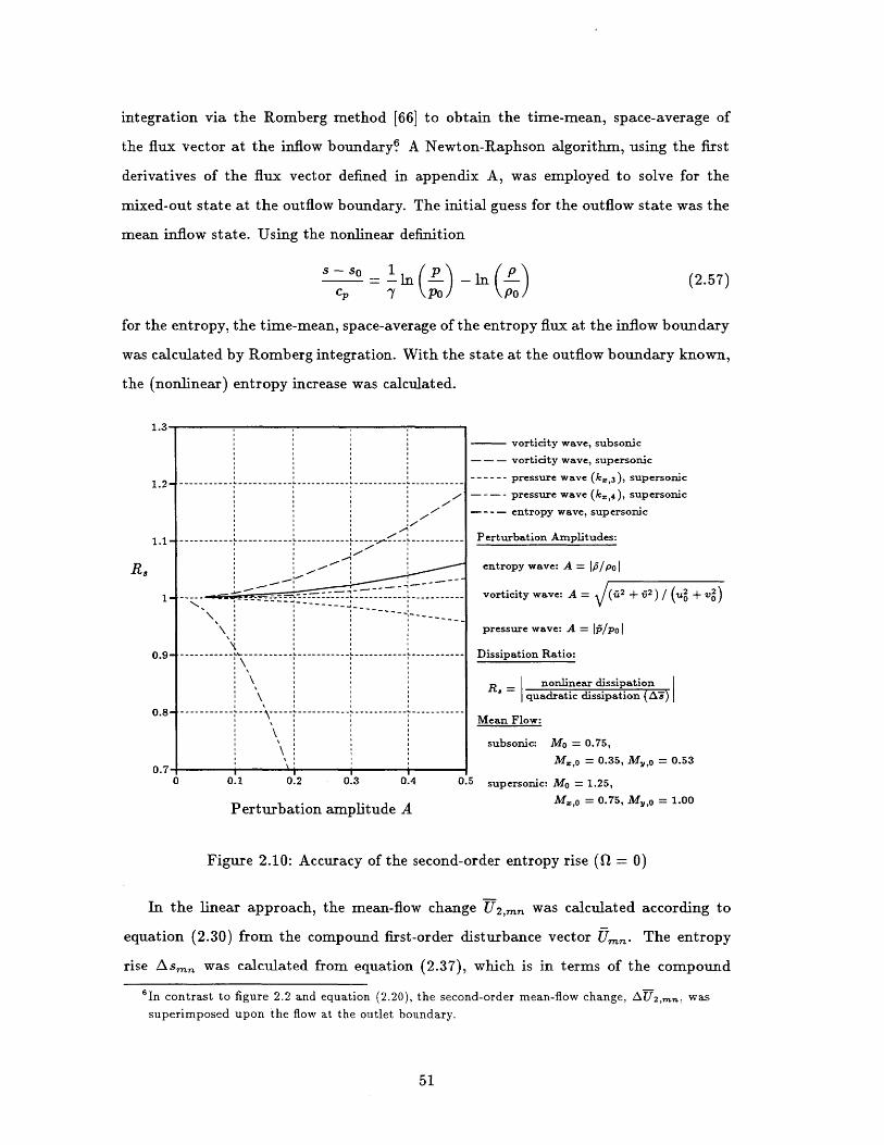
integration via the Romberg method [66] to obtain the time-mean, space-average of
the flux vector at the inflow boundary? A Newton-Raphson algorithm, using the first
derivatives of the flux vector defined in appendix A, was employed to solve for the
mixed-out state at the outflow boundary. The initial guess for the outflow state was the
mean inflow state. Using the nonlinear definition
s-so 1 p\ p= - -ln (- - n - (2.57)
CP 7 PO PO
for the entropy, the time-mean, space-average of the entropy flux at the inflow boundary
was calculated by Romberg integration. With the state at the outflow boundary known,
the (nonlinear) entropy increase was calculated.
1.3-vorticity wave, subsonic
--- vorticity wave, supersonic
1.2 ---------------------------------------------- pressure wave (ke,3 ), supersonic
- - - - pressure wave (k,, 4 ), supersonic
--- entropy wave, supersonic
- ------------------------------------- --------------- Perturbation Amplitudes:
R 8 entropy wave: A = p/POl1
- --- -------L ------- vorticity wave: A = +~ + 2 ( _ VO)
pressure wave: A = IppI
0.9 - ----------- % ----------- ------------- ----------- ---------- Dissipation Ratio:
nonlinear dissipation\ quadratic dissipation ('E)5
0.8 ------------ - -- ---- ----------- ----------- -----------Mean Flow:
subsonic: MO = 0.75,
M0,O = 0.35, MV,O = 0.530.7
0 0.1 0.2 0.3 0.4 0.5 supersonic: Mo = 1.25,
Perturbation amplitude A M.,o = 0.75, MV,O = 1.00
Figure 2.10: Accuracy of the second-order entropy rise (Q = 0)
In the linear approach, the mean-flow change U2,mn was calculated according to
equation (2.30) from the compound first-order disturbance vector Umn. The entropy
rise Asm was calculated from equation (2.37), which is in terms of the compound6 1n contrast to figure 2.2 and equation (2.20), the second-order mean-flow change, AU2,,m., was
superimposed upon the flow at the outlet boundary.
51

disturbance vector, and from equation (2.38), which is in terms of the individual waves
making up the disturbance vector.
1.3
vorticity wave, subsonic
-- vorticity wave, supersonic
1.2----------------------- -------------------- --------------- pressure wave (k., 3), supersonic---- -pressure wave (ke,, 4), supersonic
- - - - entropy wave, supersonic
1.1- -------------------- --------------------------------- Perturbation Amplitudes:
R, entropy wave: A = Ip/polI
1 -- vorticity wave: A f (i2
()!U2v
pressure wave: A = p/po
0.9- ----------- --------- ----------- ---------- ---- - Dissipation Ratio:
Rnonlinear dissipationR= =\ quadratic dissipation (aM)
0.8 - ----------- ----- - ----------- ----------- -----------Mean Flow:
subsonic: Mo = 0.75,
M,_ = 0.35, M,,0 = 0.53
0 0.1 0.2 0.3 0.4 0.5 supersonic: Mo = 1.25,
Perturbation amplitude A M1,o = 0.75, M,,0 = 1.00
Figure 2.11: Accuracy of the second-order entropy rise (Q = 4)
Comparing the results from both approaches, the result for the mean-flow change
(2.30) and the second-order entropy rise (2.37,2.38) were confirmed. For small wave
amplitudes, the results from both approaches were identical regardless of the mean flow
state and the composition of the disturbance vector. Since the mean flow-change is a
vector quantity, it is difficult to present in a diagram. The entropy rise, however, is a
scalar quantity and can easily be plotted. Figures 2.10 and 2.11 show the accuracy of
the second-order entropy rise calculated from equation (2.38) versus the perturbation
amplitudes of the disturbance for reduced frequencies of Q =0 and Q =4. The vari-
able R, is the ratio of the nonlinear entropy rise over the entropy rise calculated from
equation (2.38). Only one disturbance, i.e. a single entropy wave, a single vorticity
wave, or a single pressure wave, was entering (or leaving) the control volume in the
cases presented in figures 2.10 and 2.11. In the most general case, the model has ten
degrees of freedom. They are the mean Mach numbers M,o and M,,0 , the reduced
52

frequency D, four perturbation amplitudes, and three relative phases. The choice of a
single disturbance for figures 2.10 and 2.11 is (necessarily) arbitrary, but allows one to
judge the degree of nonlinearity of the Euler equations and the range of applicability of
the linear/quadratic analysis (if the accuracy requirement is known).
2.7 Mixing Loss at Steady Interfaces in CFD
The asymptotic analysis presented in section 2.3 can be used to investigate the mixing
loss at a steady interface in a (viscous or inviscid) simulation. A viscous simulation of
a highly loaded, transonic high-pressure turbine stage, called the ACE turbine stage,
which has been tested at MIT [50] and Oxford University [52, 541, was chosen to illustrate
the mixing loss. The simulation was performed with the CFD-code UNSFLO by Giles
[5, 6, 7, 67]. In the freestream, it uses an explicit Lax-Wendroff scheme to solve the two-
dimensional, unsteady (compressible) Euler equations on an unstructured grid composed
of triangular or quadrilateral cells. Around the blades, it uses the Thin-Shear-Layer
approximation of the Navier-Stokes equations to model viscous effects in boundary
layers. Its quasi-3D capability allows it to account for a varying streamtube thickness;
arbitrary pitch ratios can be handled with a time-inclined computational domain.
A detailed computational account of the (inviscid) stator/rotor interaction was pre-
sented by Giles [6]. Figure 2.12 shows the static pressure contours at a particular instant
during an unsteady viscous simulation. In the unsteady simulation, the stator and the
rotor row are separated by an axial gap of about 40% rotor axial chord. The outflow
of both the rotor and the stator row are supersonic, producing weak oblique shocks at
the trailing edges. An oblique shock wave, originating at the nozzle guide vane trailing
edge, first hits the downstream rotor around the crown of the suction surface and is re-
flected from there. Subsequently, it moves forward to the leading edge with the reflected
portion impinging on the adjacent pressure surface and being reflected to the suction
surface, once more. Upon lifting off the rotor blade, the primary shock wave grows
in length until the relative motion of the blade row causes it to strike the next rotor
blade. In the meantime, its reflection off the rotor leading edge has impinged on and
53

interface
I0 0.5 1.5 2
axial location z
Figure 2.12: Static pressure contours in an unsteady simulation of the ACE turbine
stage for (t/T) = 0.7
been reflected from the nozzle guide vane suction side. Comparatively large unsteady
amplitudes are expected and have been found for this turbine stage [6].
While the flows in turbomachinery are inherently unsteady, steady simulations are
often used for routine design purposes because they are easier to implement and less
CPU-intensive than unsteady simulations. Also, a steady simulations is often performed
to provide an initial condition from which to start an unsteady simulation. In a steady
simulation, the axial fluxes of mass, momentum, and energy, defined in equation (2.18),
are averaged at the stator outflow boundary to provide uniform and steady rotor inflow
conditions. Other approaches are possible and are used in practice, but they are non-
54
C7
VR
SR <0
R 0 >g 0
see chapter4

interface
0 0.5 1 1.5 2
axial location x
Figure 2.13: Static pressure contours in a steady simulation of the ACE turbine stage
conservative, (i.e. the fluxes are not conserved across the interface,) and defy physical
interpretation. Figure 2.13 shows the static pressure contours during a steady simula-
tion of the flow through the ACE turbine stage. The shock waves originating at the
stator trailing edge are seen to vanish at the interface. There, outflow boundary condi-
tions, based on a linearized model [55] as described in section 2.1, ensure that entropy
waves, vorticity waves, and pressure waves leave the stator computational domain (al-
most) without reflections. Between the stator outflow and the rotor inflow boundary,
the waves are mixed out to provide steady rotor inflow conditions. While the equations
describing the mixing at the interface are nonlinear, the associated mixing loss can be
analyzed and understood with the help of the linear model of section 2.3.
55
VR

0.5 1 1.5 2
unsteady
- - - steady
2.5
axial location x
Figure 2.14: Entropy rise in the simulations of the ACE turbine stage
Figure 2.14 compares the time-mean mass-average of the specific entropy rise, A9,
in a blade passage for a steady and an unsteady simulation of the flow through the ACE
turbine stage. It is defined analogous to equation (2.36) as
fc [fJ (pus) I d (y/P)] d (t/ T)S(X) = 1
cpf0 Lfj (pu) d (y/P) d (t/ T)
The axial coordinate x has been non-dimensionalized by the stator axial chord. The
stator leading edge is located at x=0, the trailing edge at x=1, as is shown in figures
2.12 and 2.13. The focus here is on the steady interface; other aspects of figure 2.14 are
brought up later. Of the total entropy rise in a steady simulation, about 20% (equivalent
to A2i=0.00417) are caused by (nonphysical) mixing at the stator/rotor interface. How-
ever, the entropy rise beyond the interface is slower in the steady simulation because all
waves that could cause unsteadiness and additional loss in the rotor frame have been
dissipated at the interface already. As a consequence, the entropy rise through the stage
remains only 8% higher in the steady simulation than in the unsteady simulation.
56
0n. r,
0.020-1
0.015-
0.010-
0.005-t
0
0.
mixing loss: Aso = 0.00417- -------I ---- - -------- -- ---- ---- -- -- -- -7 ---- ------ ----- - -------
rotor crownInterface
--- -- -------- ---------- -- ------ -- -------.- 'boundari
stator trailingedge
- ------ -------- --------- ----------------------- -------- - --- --------rotor trailing
edge
rotor leading-- - - - r - -- - - - - - -- - -- ---- --- --.. -------- --------- r---------
e ge
(258)

interface
0 0.5 1 1.5 2
axial location x
Figure 2.15: Stage geometry and computational grid of the ACE turbine stage for
(t/T) = 0.7
The computational grid, see figure 2.15, along the stator outlet boundary (as well as
the stator inlet, the rotor inlet, and the rotor outlet boundary) is equally-spaced. This
facilitates the implementation of boundary conditions in a steady simulation and the
transfer of information between the blade rows in an unsteady simulation. Due to the
constant spacing, the nonuniform flow in a steady simulation can easily be decomposed
into its spatial Fourier modes along the stator outflow boundary. With the Fourier
modes known, the individual waves contained in these modes can be determined with
the help of the left eigenvectors of the linearized Euler equations defined in appendix G.
From the individual waves, the entropy rise (the mixing loss) at the interface can be
57

determined using equation (2.38). Figure 2.16 shows the contributions to the entropy
rise of individual waves of different wavenumbers along the interface.
-2-
-3-
log A9m 0I
-6-
-7-
S6 A9 13 15
circumferential wave number (ky,m/kyi)
Figure 2.16: Decomposition of the entropy rise into the wave types
(fundamental wavenumber ky,1 corresponds to the stator pitch)
[ total
Z) entropy wave kz,lmO
Avorticity wave kr,2m,,O
pressure wave k,,3m0
pressure wave k.,4mO
and wavenumbers
While it was recognized previously that the interface treatment in steady simulations
results in an entropy rise, it was assumed to be negligible [68]. Clearly, this is not true
for stages with a high level of unsteadiness, like the ACE turbine stage. The presence of
oblique shock waves introduces a relatively strong perturbation into the stator outflow
and causes a considerable entropy rise upon mixing-out. The entropy rise is not without
physical implication, though. The same entropy rise would be seen if stator and rotor
were placed infinitely far apart and the flow allowed to mix out in between.
Many factors contribute to changes in the efficiency upon variation of the gap be-
tween blade rows. In experiments by Smith [22] and Mikolajczak [23], the efficiency
increased with decreasing axial gap. In experiments by Hetherington and Moritz [24]
58
p edicted e tropy rise: Aso =0.00436
-K --
------ ---- ---------- ---- -- - - -- ------- -------------- -------
~-)K-
4 - -

it decreased with decreasing axial gap. Mixing loss can give one explanation for an
increase in efficiency with decreasing axial gaps. The entropy rise at the stator/rotor
interface of a steady simulation is equivalent to the maximum entropy rise that can
result from mixing losses.
In a steady subsonic flow, all pressure waves are of evanescent nature, as can easily
be deduced from equation (2.15). They do not contribute to the entropy rise. In a steady
supersonic flow, all pressure waves are non-evanescent and do contribute. Weak shock
waves can be modeled as isentropic pressure waves with the vector sum of propagation
velocity (speed of sound) and convection velocity along the shock front. The flow at
the stator outlet boundary of the ACE turbine stage is supersonic. From figure 2.16
and table 2.1, shock waves (pressure waves propagating downstream with wavenumber
k3,mO) are seen to account for the major part of the mixing loss. Vorticity waves and
entropy waves, primarily a consequence of the stator boundary layer, contribute the
rest. There is also a minor (negative) contribution to the entropy rise from pressure
waves propagating upstream. The flow is axially subsonic and pressure waves can travel
upstream against the flow. Since disturbances in the rotor frame do not make them-
selves felt upstream beyond the interface of a steady simulation, these must be due to
reflections from the stator outlet boundary. While the stator outlet boundary conditions
are designed to pass through waves traveling downstream, their linear nature produces
weak reflections in the presence of nonlinear phenomena like shock waves.
Table 2.1: Contributions to the entropy rise at the interface - by wave type
The linear/quadratic model overpredicts the (nonlinear) mixing loss in the simula-
tion by only 4.5%. The discrepancy is explained by the nonlinearity of the averaging
process in the presence of (all but the weakest) shock waves. Note that this behavior is
59
predicted entropy riseAT J 0.00436
Entropy waves (kx,1m) 4.3%
Vorticity waves (kx, 2m) 15.6%
Pressure waves (kx,3m) 80.9%
Pressure waves (kx,4m) -0.8%

consistent with figure 2.10, which shows that the linear model overpredicts the entropy
rise due to dissipation of downstream propagating pressure waves of finite amplitudes.
The axial Mach number M:,o and the normal Mach number My,o used for the super-
sonic cases in figure 2.10 are very close to the Mach numbers found at the stator outlet
boundary in the steady simulation of the ACE turbine stage. Weak shock waves can
be modeled as isentropic pressure waves with the vector sum of local convection ve-
locity and local propagation velocity (speed of sound) pointing along the shock front.
From table 2.1, downstream propagating pressure waves are seen to be the dominating
perturbation at the stator outflow boundary. Given the large amplitude of the dis-
turbance at the stator outlet, the ACE turbine stage represents a difficult test for the
linear/quadratic model and it exhibits surprising accuracy.
Table 2.2 lists the contributions of different wavenumbers to the entropy rise, in-
dependent of the wave type. The fundamental wavenumber along the interface, ky,1 ,
corresponds to a wave with one period per (stator) blade pitch. The importance of
higher harmonics is due to the presence of oblique shock waves.
predicted entropy rise A- 0.00436
wavenumber k, 1 49.9%
ky,2 32.5%
ky,3 9.2%
ky,4 5.2%
ky'5 2.4%
all higher modes 0.8%
Table 2.2: Contributions to the entropy rise at the interface - by wavenumber
60

2.8 Summary - Unsteadiness and Loss
This chapter presented a rigorous mathematical argument relating the dissipation of
unsteady waves in a uniform mean flow to the resulting entropy rise. It is the first ap-
plication of an asymptotic analysis to this problem and represents the first work clearly
identifying the separate contributions to the entropy rise stemming from simultaneous
linear disturbances.
The accuracy of the linear/quadratic model was evaluated by comparison to a non-
linear approach. Also contained in this chapter is the first detailed analysis of the
mixing loss at the stator/rotor interface of a steady simulation. The magnitude of the
mixing loss predicted by the asymptotic analysis is in excellent agreement with the
(nonlinear) simulation.
This chapter also pointed out another fact that seems to have been generally over-
looked. As a consequence of the mixing loss at the stator/rotor interface, the steady
simulation of a stage can have a lower efficiency than the corresponding unsteady sim-
ulation. The mixing loss at the interface is the same as the one which would occur for
an infinite gap between the rotor row and the stator row, providing an explanation for
a loss increase in turbomachinery with increasing blade row gaps.
61
Chapter 3
Unsteady Circulation Loss
A turbomachine blade row moves through a flow field disturbed by inflow distortions,
potential interactions with adjacent blade rows, shock waves, wakes, vorticity shed at the
upstream blade rows, and propagating pressure waves. Furthermore, blade movement
(in flutter or forced-response problems) leads to periodic changes in the magnitude
and the direction of the incoming flow vector relative to the blade. As a consequence,
the blade circulation changes in a periodic manner and, in accordance with Kelvin's
Circulation Theorem, vorticity is shed at the trailing edges and convected downstream
with the mean flow. The transfer of energy from the mean flow into kinetic energy
associated with unsteady vortex sheets is regarded as a loss in accordance with chapter 2.
This loss mechanism was first considered by Keller [10], who calculated the average
kinetic energy in the vortex sheets trailing a single blade row in an incompressible flow as
a function of the unsteady c irculation amplitudes and the stage geometry. He estimated
the circulation amplitudes at 5% of the steady circulation and related the average rate at
which energy is transferred into the vorticity field to the steady power required to turn
the rotor. His results indicate that, on average, the specific secondary kinetic energy is
between 0.4% and 1% of the steady specific work absorbed or developed by the rotor,
with the exact value depending on the stage geometry.
Sears and Kemp [70] used thin-airfoil theory to calculate the unsteady lift acting
on a rotor row subject to the wakes of an upstream stator row. Fourier decomposition
of the velocity perturbation and subsequent application of results presented in earlier
papers [12, 13], allowed them to calculate a slowly converging series of unsteady lift co-
efficients. In [11], they used thin-airfoil -theory, as presented in earlier papers [15, 14], to
calculate the circulation amplitudes and extended the approach to an elementary stage
62

with potential interactions between blade rows. This approach, while enabling them
to calculate the circulation amplitudes, limited them to incompressible flow, blades of
zero thickness and camber with the mean flow nearly in the blade direction, i.e. lightly
loaded blades. Thus, the airfoils are more representative of compressor blades than tur-
bine blades. Furthermore, they had to specify the steady lift distribution on the blades.
They found that the unsteady circulation amplitudes are, in general, substantially less
than those assumed by Keller. As a consequence, the secondary kinetic energy is less
than what was found in [10]. Also, the circulation amplitudes were much larger for the
upstream blade row (in a single stage) than for the downstream blade row. This was
attributed to the importance of the velocity field at trailing edge to the blade circulation.
In another approach for incompressible flows, Hawthorne [16] used lifting-line theory
to calculate the rate of energy transfer. He found values which are essentially in line
with those of Keller.
Korakianitis [71] used a CFD-code (UNSFLO) to determine the unsteady forces act-
ing on rotor blades in subsonic flow. He systematically varied the geometric parameters
of rotor blade rows in an effort to provide design data that predicts the unsteady blade
forces in response to incoming viscous wakes and potential disturbances. In the cases
considered, he found average unsteady forces and moments which are typically between
90% and 100% of the mean values. Giles [6] reported a 40% peak-to-peak variation in
the rotor lift for a transonic high-pressure turbine stage under the influence of unsteady
shock wave/blade row interaction.
In this work, the circulation amplitudes are the results of numerical simulations,
which allows one to obtain unsteady circulation amplitudes for arbitrary blade and stage
geometries, steady lift distributions, and Mach numbers. Kelvin's Circulation Theorem
is valid even in compressible flows, provided the flow is homentropic. Eliminating the
need to estimate the circulation amplitudes or to deduce them from thin-airfoil the-
ory, results in a realistic measure for the importance of this loss mechanism in modern
turbomachines. The work proceeds along the lines of [10]; it considers a single blade
row, its circulation variation and the associated trailing vorticity only. Wake/rotor and
63

rotor/stator interaction cases are considered. In wake/rotor interaction cases, experi-
mental data is used to model the wake.
3.1 Analytical Theory
3.1.1 Single Airfoil
Figure 3.1 shows an airfoil experiencing an unsteady lift and circulation due to either
its own motion or the imposition of an external disturbance. The coordinate system
has been chosen such that the freestream velocity, U,, and the wake are aligned with
the x-axis.
y
U00
Figure 3.1: An isolated airfoil with an unsteady lift and circulation
Let the circulation on the airfoil be described by a steady component plus sinusoidally
varying, unsteady components.
00 00
F (t) = F + E Im (t) = Y + Z me~'"(WMt-'M) (3.1)m=1 m=1
The variable <Pm denotes the phase angle of the mth temporal mode. In the above
equation, and in the remainder of this chapter, it is the real part of any quantity, that
is implied by complex notation.
64

The strength of the unsteady vortex sheet shed at the trailing edge is determined
by the condition that the sum of bound and shed vorticity remain constant. This is
a consequence of Kelvin's Circulation Theorem which is valid in any compressible flow
that is inviscid, barotropic, and has only conservative body forces acting on it. In a
barotropic flow, the density is a function of the pressure only. The barotropic condition
can be replaced by the requirement of a homentropic flow because a homentropic flow
is also barotropic. If any of these conditions is violated, source terms appear in Kelvin's
Circulation Theorem, and the sum of shed and bound vorticity is no longer constant.
The strength of the vortex sheet (x, t), which is convected with the mean flow, is
related to the rate of change of the circulation by
S(X, t) = -' Id[(t - . (3.2)Uoo dt U01
There are, at this point, two principal objections to this model. First, a single vortex
sheet suffers from the Kelvin-Helmholtz instability to small perturbations and tends to
roll up into discrete vortices. Second, due to the circulation bound to the airfoil, a simple
convection of the vortex sheet is a poor model in the nearfield. The first problem is
solved by noting that the kinetic energy of an isolated vortex sheet undergoing inviscid
roll-up is invariant. The second problem exists in the nearfield only; in the farfield, the
influence of the steady circulation is limited to an axial and circumferential offset, which
is without consequence for the amount of secondary kinetic energy present.
A frame of reference convected with the mean flow, in which the flow appears steady, is
introduced by
X = X - U00t
and y=y. (3.3)
Equation (3.2) may now be written in the form
Sm=1
65

where the reduced frequency km is defined by
km W MC (3.5)U00
The variable c denotes the airfoil chord.
In the stationary frame, the linearized potential equation, i.e. the equation for
the perturbation potential describing the flow field induced by the vortex sheet far
downstream of the trailing edge, is
I a+ U(--+) + V2 = 0, (3.6)a2 (at ax
where a denotes the speed of sound. Unsteady and convective contributions in equa-
tion (3.6) are eliminated by the shift in the frame of reference; all that remains is
-2 + - = 0. (3.7)
In the convected frame, the flow perturbation satisfies the equations for steady, irrota-
tional, and incompressible flow, regardless of the freestream Mach number. Due to the
linear nature of equation (3.7), the principle of superposition can by applied. Far down-
stream of the trailing edge, where the influence of the bound circulation is negligible,
the perturbation potential &m associated with the mth mode is
b = exp ikm- exp {-km ', for y > 0,
and Om = A exp ikm- exp +km -I for < 0. (3.8)
The values of A+ and ka are determined from the matching conditions at y = 0. First,
the jump in the tangential velocity perturbation ii across the vortex sheet must equal
the strength of the vortex sheet.
um (i, 0+) - im (i, 0-) = jm (i) (3.9)
This leads to
im (0+) _ im (0~) m > i -km j m. (3.10)CP+-A
66

Second, for the problem under consideration, there must be no jump in the normal
velocity perturbation v.
Fm (,10+) - UM (i, 0~) 0 (3.11)
From equation (3.11) follows
&m (0+) - Vm (0) = 0 - - - = 0. (3.12)
Combining the two results above gives
= - - = 2 e . (3.13)2
The average rate at which kinetic energy is transferred from the mean flow to the
unsteady motion associated with the shed vorticity is keUm. Due to the orthogonality
properties of trigonometric functions, summarized in appendix B, the principle of su-
perposition can be used. The kinetic energy in the convected frame can be calculated
mode by mode and summed subsequently. The average specific kinetic energy per unit
wake length and depth of the mth mode, kem, is determined by integrating the kinetic
energy over one wavelength in the i-direction and from 0 to oo in the y-direction.
k + 27rc/km 1imem ]J" J f [3 (im)]2 + [g? (m)]2} di dp
27rc _. 2
km +00 2-7c/km, 2 + 2
= k j+ km 1 {[ ' d() dy (3.14)
The symbol R denotes the real part of a complex quantity. With the help of equation
(2.31) in subsection 2.3.1, the final result for the average kinetic energy associated with
the shed vorticity becomes
ke 8 km -m .)(3.15)M=1
It is the average specific kinetic energy, ke, which, in accordance with equation (2.38)
of subsection 2.3.2, is related to the entropy rise upon mixing. There, the entropy rise
was summed over all temporal and spatial modes, In the application here, the spatial
Fourier-decomposition of the convected unsteady velocity field is not known explicitly.
If the spatial Fourier-decomposition of the unsteady velocity field were carried out and
the secondary kinetic energy of one temporal mode summed up by spatial modes, the
67

result would be the same as in equation (3.15) by virtue of the orthogonality properties
of sines and cosines (appendix C). It is important to point out that the entropy rise
is independent of the frame of reference and, in particular, the Mach number of the
freestream. Thus, the approach taken in [10] can be extended to compressible flows.
3.1.2 Cascade
Figure 3.2 shows an analogous situation for a cascade in which every blade is experi-
encing an unsteady lift and circulation due to the imposition of an external disturbance
induced by the upstream blade row in an elementary stage.
VR
n=1
UO
"PO (/n =0
Figure 3.2: A cascade with an unsteady lift and circulation
The coordinate system has been chosen such that the mean downstream velocity,
Uo, is in the i-direction and the wake of the nth blade lies along y = nP. P is the
68
y P
Y
x
O

standard pitch, P the rotated pitch defined as P cos a, P* the standard pitch of the
neighboring blade row, and a the angle between the wake and the axial direction.
Suppose that the circulation of the nth blade is given by
00 00
P (t) = n + I"i (t) einl3" = 7 + E Pme4W"t-n/m- ", (3.16)m=1 m=1
with /3m being the inter-blade phase angle for the mth mode. The frequencies Wm
correspond to the blade passing frequency and its harmonics
VRWm = m wf = 27r m , (3.17)
where VR is the rotor speed. The inter-blade phase angle is obtained from the difference
in pitch of the blade rows as
3m = 27r m sign (VR). (3.18)
Thus, the unsteady vortex sheet strength along the nth wake is given by
1 d [ / x-nPsina'1( )= tn [ - . (3.19)
nZi) UO td t UO
With equation (3.16), this can be expressed in the form
00 {(320?n (i) = r km expt i km+ nm+ Pm .(3.20)
m=1
The inter-wake phase angle of the mth mode, #m, is defined by
-m= - 3 m kP sm a = - A. tan a, (3.21)2 2 2 c 2
with the reduced frequency Am given by
1 PAm = -km-. (3.22)
2 c
The convected coordinate ' and the reduced frequency km are defined as before, with
U0 0 replaced by UO, and the airfoil chord replaced by the blade axial chord. The spatial
periodicity condition for the perturbation potential of the mth temporal mode is
M PZ ) = m(' ) e'. (3.23)
69
The matching conditions at the zeroth wake are identical to the conditions used for a
single airfoil, equations (3.9) and (3.11). For 0 < y < P, the potential can be written as
rm (j, 9) [ [ cosh km -Am + B sinh km -A m ) exp ki (km )+ }.
Using the periodicity condition (3.23) to relate the velocities at (i, 0-) to those at
(X, P-), the matching conditions give the following equations:
(Am cosh Am - Bm sinh Am) e+im/2 - (Pm cosh Am -
(Am cosh Am + tm sinh Am) e +i4m/ 2 + (Am cosh Am -
These two equations can be written in matrix form as
Bm sinh Am) e-i4m/2 = Pmeiw'
Bm sinh Am) e-i3m/2 = 0 (3.25)
+i cosh Am sin kp-i s2[i isinhAmcos 4-
.A
F3
- sinh Am cos Z!2
+1i cosh Am sin - ) 20
and solved to yield
.- i cosh Am sin ptoAm = - 2 - r ce-
Asi2 2 0- + sinh2 Am
= sinh Am cos E2.and Bm I -- 2 mei~n2 sin2 3 + sinh2 Am2
Hence, the solution for 0 < < P is
~ Tm/2c Ly.nm-m = - Pm2C [cosh Am sin-
sin2 4- + sinh2 Am i ch 222
+ sinh Am cos - sinh2 (km- Am )
cosh (km- -C
exp
kml'm/2c
sin2 4- + sinh 2 Acosh Am sin -s
2cosh (k- -
+i sinh Am cos 2 sinh (km
and
kmrm/2c
sin2 P7 + sinh 2 Ami cosh Am sin
2sinh km-Y - Am)
C
+ sinh Am cos cosh2 (km exp i km
70
(3.24)
(3.26)
(3.27)
Am)
+ + Om , (3.28)
Am)
- Am ) exp { + + <pm) , (3.29)
+ + m . (3.30)
e
X
i k( C
i km
- Am ]
The corresponding average kinetic energy per unit mass is
I-. 1 kf 27rc/k,, 1k j j-rc/ 1 [-2 (am) + R2 (;m)] dy dX
2
kmm/4c 2/Om 23mcosh2 Am sin2 + sinh2 Am cos2 - X
sin2 4. + sinh2 A 2 2I
22
x - )cosh km - Am + sinh km- c Am dy
(kmrm /4c)2 P- cosh 2 km-y - Am dy
sin 2 J_ + sinh2 I fo
I r. 2 A sinh Am cosh Am (3.32)
()31
4 kpa sin2 L + sinh2 Am
which can be shown to coincide wit f sueto [.3.. Then this energy is dissipated
later, the resulting mass-average entropy increase is
_ y - 1 (m 2 Am sinh Am cosh Am4 (Pao sin2
!!4 + sinh 2 Am
2
in accordance with equation (2.38) of subsection 2.3.2. The corresponding total pres-
sure drop
_ y rm 2 A, sinh Am cosh AmA~em (3.33)
4 (Pao) sin2 0- + sinh2 Am
is obtained from equation (2.47).
3.1.3 Cross-Induced Kinetic Energies
The shedding of vorticity at the trailing edge in response to circulation variations is
ultimately caused by the presence of unsteady perturbations. Vorticity waves, in the
form of wakes being convected with the mean flow, and pressure waves, in the form of
weak shock waves, are found to be of equal importance in the following section. For
very small axial gaps, evanescent potential interactions can be significant, too.
If shedding of vorticity is being caused by the presence of weak shock waves or
the evanescent potential field of the upstream blade row in an elementary stage, the
entropy rise calculated with the kinetic energy (3.31) only is correct. As was shown
71

in subsection 2.3.2, propagating pressure waves and evanescent potential fields do not
couple with vorticity waves upon dissipation. A very weak shock wave can be thought
of as being composed of isentropic pressure waves with the vector sum of the local
convection velocity and the local speed of sound pointing along the shock front.
Vorticity waves (wakes), however, can be both cause and consequence of unsteady
voticity shedding at the trailing edge. The vorticity waves being convected through a
cascade and causing a periodic circulation variation are of the same frequency and axial
wavenumber as the vorticity shed at the trailing edge. In the calculation of the secondary
kinetic energy (3.31), the velocities induced by the vorticity convected through the blade
row and the kinetic energy associated with it, are not accounted for. There are three
reasons for the neglect of these cross-induced contributions.
First, it is difficult to account analytically for cross-induced contributions in the com-
plex geometries and flow fields that will be considered. The vorticity convected through
a cascade adds to, or subtract from, the self-induced secondary kinetic energy (3.31)
(depending on the phase relationship between convected and shed vorticity), giving
the self-induced kinetic energy the character of a mean value. The self-induced kinetic
energy is associated with velocities induced by a blade row's own trailing vortex sheets.
Second, for potential rotor/stator interaction in an elementary stage, the analysis by
Kemp and Sears in [70] suggests that the cross-induced contributions (from the vorticity
shed at the trailing edge of the upstream blade row) to the secondary kinetic energy
beyond the downstream blade are of the same size as the self-induced contributions.
For the upstream blade row, they were found to be negligible. The differing relative
magnitudes of self-induced and cross-induced contributions were explained by the cir-
culation amplitudes; the upstream blade rows showed unsteady circulation amplitudes
which were a factor of ten larger than those of the downstream blade rows. In the simu-
lations performed here, the circulation amplitudes were of the same order of magnitude,
suggesting a second rationale for neglecting cross-induced contributions.
72
Third, in wake/rotor interaction, most of the wake unsteadiness originating at the
trailing edge of the upstream blade row is in the lowest circumferential wavenumber.
As a consequence, most of the unsteadiness in the (frame of reference of the) down-
stream blade row is at the fundamental (blade passing) frequency. In the convected
frame beyond the trailing edge of the downstream blade row, most of the unsteadiness
associated with the convected vorticity is therefore found at the fundamental stream-
wise wavenumber. While the shed vorticity induces a velocity field continuous in the
streamwise (i-)direction, it introduces a discontinuity in the normal (y-)direction.
This implies that the shed vorticity has energy in discrete normal wavenumbers spread
over an infinite range, even if the incoming unsteadiness has its energy confined to the
blade passing frequency. Due to the orthogonalities of sines and cosines, summarized
in appendix C, there is no crosscoupling between the incoming convected vorticity and
the higher harmonics of the shed vorticity in the normal (y-)direction. It is therefore
legitimate to ask how much of the secondary kinetic energy is in the higher spatial
harmonics. To that end, the normal Fourier modes of the velocity field described by
equations (3.29) and (3.30) have to be found. For the mth temporal mode, the normal
wavenumbers downstream of the rotor are
kn = .+21r (3.34)
For simplicity, and without loss of insight, it will be assumed that 3r is an integer
multiple of 27r and that 'Pm = 0.
O3m = 2j 7r, j = 1, 2,... (3.35)
If the inter-wake phase angle were not taken to be zero, the determination of the Fourier
coefficients would involve a summation over a finite number of blades. This is because
the potential (3.28) is valid only over an interval of extent P, while the integration to
obtain the Fourier coefficients has to be carried out over an interval of periodicity. The
Fourier coefficients are:
Umn'S - 2 sin kn 1)d -2(-l) p k 2 sin (km) (3.36)(1~~~/c)~~ 1 sn cI \c= m n \C
73

mn 2 C (P/c Vmn,c = , Cos kn- )
(P/c c
1.4-
1.2-
1
0.8-
Amplitude
0.4-
0.2-
1 2 3 4 5 6
2 1/c # pUmn,c = , (Cos kJ u d )- = 0 (3.37)
2 P/C pVmns = ( P/) sin kn-') d - = 0 (3.38)
P / c) fo e c
d(- = -2(-1)ll (+) k2 cos km- (3.39)+ k C
6 8 9 10
-V-mn,c
ElA
Am= 10Am= 15
11
Harmonic #
Figure 3.3: Relative magnitude of the spatial harmonics in the shed vorticity wake (first
harmonic corresponds to the pitch of the upstream blade row)
Figure 3.3 shows the relative magnitude of the velocity harmonics um,, and vmn,c,
nondimensionalized by the respective first spatial harmonic, with the reduced frequency
Am as a parameter. Note that for higher harmonics (large wavenumbers) Umn,s 1/kn,
which is consistent with the discontinuity of the streamwise velocity perturbution U at
the vortex sheet. Since the normal velocity perturbation ii is continuous everywhere,
one finds Vmn,c ~ 1/k2 for large wavenumbers. The quadratic decay is mandated by
the discontinuity of its derivative at the vortex sheet. This is easily deduced from the
potential equation in the form (al/) = - (hi/d). From equations (3.36) and (3.39),
74
---- - - -- - - -- - - - - - - - - -- - ---'- - - - - - - - - - - -
- - ------------------------------------A
- --- -- ---- ---A
---- ------- -4-- - - -- - -
--- --- ------ -- --------- ---- ----T Z Q -- ----L ----
------- ~. -- --'-- ------7 ----- --- ----

one can calculate the spatial average of the secondary kinetic energy associated with a
wavenumber kn.
Ir 2 k 2kemn = - - 2
k +kn 1 + (7r/Am) 2 2
1"
0.8-
rTm
0.6-
0.4-
-1 -0.2 0.6 1.4 2.2
(3.40)
log (2Am)
Figure 3.4: Relative amount of kinetic energy in higher spatial harmonics
Figure 3.4 shows the ratio
Zn=2 kemnrm = __-. (3.41)E', kemn
versus the governing parameter Am. Even in the limit Am- 0, i.e. for zero reduced fre-
quency, there is a finite amount of secondary kinetic energy in higher spatial harmonics.
The limiting case for Am= 0 leads to a value of
1 _ 6rm = 1 - - 3 9.2%. (3.42)
E',= (1/n2) T2
In the cases considered in the next section, a typical value of Am is 5 and roughly 64%
of the secondary kinetic energy is found in higher spatial harmonics.
75
--- -- ---------- ---- --- ---- ------- --- --- --- -- --------
--- - - - - - ----------- ------ ---------- --------- -- ----- - -------- --------
.

3.2 Results - Unsteady Circulation Loss
The analytic model described in the previous section was applied to a number of blade
rows and stages. The amplitudes of the unsteady circulation were calculated with the
CFD-code UNSFLO by Giles [5, 6]. The simulations were run until the flow was periodic;
then 50 instantaneous flow solutions equally-spaced in time were stored, from which the
circulation amplitudes were determined. For a single blade row, unsteadiness due to
upstream blade rows, (i.e. viscous wakes and potential disturbances), was modeled
at the inflow boundary. Incoming wake models and potential disturbance models are
described in [67].
3.2.1 Single-Stage, Large-Scale Turbine No. 2 at Cambridge
Hodson [69] conducted measurements of wake-generated unsteadiness in the rotor of a
large-scale, low-speed, single-stage, air-driven turbine. As detailed in [69], the stage is a
free-vortex design with zero exit swirl and high reaction. The uniform axial velocity at
the stage inlet combined with radial equilibrium results in no curvature in the meridional
plane. The flow at midspan can thus be regarded as two-dimensional. The 51 rotor
blades are separated from 36 stator blades by an axial gap of about one rotor axial
chord. In [42], Hodson computed the two-dimensional wake/rotor interaction with the
data for the modeling of the incoming wake taken from [69].
Input Parameters Others
Inlet Flow Angle 2.10 Outlet Flow Angle a -66.80
Exit Static Pressure 0.8956 Inlet Mach Number 0.14
Isentropic Exponent 1.4 Outlet Mach Number Mo 0.40
Stator Pitch/Rotor Pitch 1.417 Rotor Pitch 0.982
Rotor Speed VR 0.3104 Reduced Frequency k1 3.45
Table 3.1: Input parameters for the simulation of the Cambridge No.2 turbine
76

The input parameters for the simulation are in table 3.1. Pressures have been
nondimensionalized by the inlet stagnation pressure, lengths by the rotor axial chord
and velocities by the inlet stagnation speed of sound. Outlet flow angles as well as
inlet and outlet Mach numbers are time-mean mass-averages in the frame of reference
moving with the corresponding blade row. The wake model was identical to the one
used by Hodson in [42]. The maximum velocity defect and the wake width were chosen
such as to replicate the maximum velocity and the momentum deficit in figure 4 of [69].
No effort was made to account for the viscous decay of the wake in the experiment. In
the absence of information about a potential disturbance acting on the rotor, it was not
modeled. Given the large axial gap, it can be expected to be insignificant.
Wake only
Wake Velocity Defect in [%] 4.6
Wake Width/Stator Pitch in [%] 30
Wake Angle (stator frame) 65.00
r,/r in [%] 0.67
Entropy Rise A-1 1.66 x 10⁻⁶
Total Pressure Drop' -Apt 5.80 x 10⁻⁶
Efficiency Drop -Ar7.,,E7s,E,D ~ 0.04%
Table 3.2: Unsteadiness parameters and results for the Cambridge No.2 turbine
The result of the simulation is summarized in table 3.2. With the harmonics of
the circulation known, the entropy rise and the total pressure loss are obtained from
equations (3.32) and (3.33), respectively. Section 2.5 relates the total pressure drop to
the drop in the isentropic efficiency. Higher harmonics of the circulation (P., m > 1) did
not contribute significantly and are not included in the above table. In the remainder
of this chapter, higher harmonics have been found to be insignificant, i.e. more than a
factor of 10 smaller than ]1, if they are not listed.
'Total pressure drop as defined here is not used in low speed flows. Instead, the total pressure dropis nondimensionalized by the dynamic head. It is used here to be in line with the chain ofreasoning in chapter 2. The important measure is the efficiency drop.
77

3.2.2 Large Scale Rotating Rig (LSRR) at UTRC
The second case is a simulation of the flow through the rotor of a large-scale, axial-flow
turbine model investigated experimentally by Joslyn, Dring, and Sharma [72]. It is a
one and one-half stage turbine model consisting of 22 first vanes, 28 first blades, and
28 second vanes, representing the first three blade rows of the high-pressure turbine
of a high bypass-ratio aircraft turbine. The Reynolds number of 5.6 x 10⁶ and the
absolute and relative flow angles are typical for current high-pressure turbine airfoils.
The important input parameters for the simulation of the flow through the rotor are
summarized in table 3.3.
Input Parameters Others
Inlet Flow Angle 48.90 Outlet Flow Angle a -65.50
Exit Static Pressure 0.975 Inlet Mach Number 0.124
Isentropic Exponent 1.4 Outlet Mach Number Mo 0.200
Stator Pitch/Rotor Pitch 1.2727 Rotor Pitch 0.9578
Rotor Speed VR 0.1137 Reduced Frequency k, 2.92
Table 3.3: Input parameters for the LSRR simulation
In a first simulation, the incoming unsteadiness consisted of wakes only. The wake
profile was Gaussian as described in [67]; the wake width and the maximum velocity
defect were chosen to match the maximum velocity defect and the momentum defect at
midspan downstream of the first vanes, which were documented in figure 6 of [72].
In a second simulation, a potential disturbance was superimposed upon the wake
disturbance. The unsteady pressure amplitude of the potential disturbance was cho-
sen such that it causes a potential velocity perturbation resembling the one shown in
figure 6 of [72]. However, while the measurement station in the experiment is ap-
proximately 0.52x (axial chord) upstream of the rotor leading edge, the location of the
potential disturbance was set at 0.15x(axial chord) in the simulation. Otherwise, the
influence of the incoming potential disturbance on the rotor would have been negligible
due to its strong exponential decay at low Mach numbers. Also, depending on the lo-
78

cation of the inflow boundary, where the potential disturbance is prescribed, it can add
to or subtract from the wake effect on the circulation. The results of both simulations
are in table 3.4.
Wake Wake+Potential
Wake Velocity Defect in [%1 15 Pressure Disturbance 3 x 10- 3
Wake Width/Stator Pitch in [%j 0.10 Disturbance Location -0.15
Wake Angle (stator frame) 68.50
P1 /J in [%] 0.57 r 1 /r in [%] 0.68
Entropy Rise A-91 1.23 x 10⁻⁵ A 1.72 x 10⁻⁵
Total Pressure Drop -A-p, 1 4.32 x 10⁻⁵ -Apt, 6.01 x 10⁻⁵
Efficiency Drop -ATs,E/77s,E,D 0.11% -A77s,E/?7s,E,D 0.15%
Table 3.4: Unsteadiness parameters and results for the LSRR
3.2.3 Cold Air Turbine Stage at the DFVLR
Binder [73] used the L2F technique to measure the flow in cold air turbine test facility.
The stage had 20 stator blades, 31 rotor blades, and an axial gap of 113% rotor axial
chord; it was a scaled version of the first stage of an helicopter gas turbine.
The flow in the low aspect ratio, high hub-to-tip ratio stage was weakly transonic
and showed a wake with a velocity defect of 6.5% and an angle of 700 at midspan,
50% rotor axial chord upstream of the rotor leading edge. Potential interactions at
this axial gap were found to be negligible. In the simulation, the unsteadiness at the
rotor inlet boundary consisted of wakes only. The input parameters for the simulation
are in table 3.5. Based on the velocity distribution at the rotor inlet measuring plane,
documented in figure 5.7 of [73], a sinusoidal wake model, as described in [67], with a
maximum velocity defect of 6.5% in the stator frame of reference was chosen.
79

Input Parameters Others
Inlet Flow Angle 46.70 Outlet Flow Angle a -620
Exit Static Pressure 0.699 Inlet Mach Number 0.43
Isentropic Exponent 1.27 Outlet Mach Number Mo 0.65
Stator Pitch/Rotor Pitch 1.55 Rotor Pitch 0.822
Rotor Speed VR 0.5765 Reduced Frequency k1 4.25
Table 3.5: Input parameters for the DFVLR turbine simulation
Note that this case does not strictly satisfy the condition of homentropic flow re-
quired by Kelvin's Circulation Theorem (in compressible flow). Since the flow is not
incompressible, as in the previous two cases, a viscous wake consists of a vorticity wave
accompanied by an entropy wave.
Wake only
Wake Velocity Defect in [%] 6.5
Wake Angle (stator frame) 700
rI1 / in [%] 2.83
Entropy Rise A31 3.56 x 10⁻⁴
Total Pressure Drop -A-pj 1.67 x 10⁻³
Efficiency Drop -Ar/s,E/tls,E,D 0.24%
Table 3.6: Unsteadiness parameters and results for the DFVLR turbine
80

3.2.4 ACE Turbine Stage
This subsection shows the results obtained for a highly, loaded transonic high-pressure
turbine stage, which has been investigated at MIT [50] and Oxford University [52, 54]. In
the experiments, the objective was to closely simulate all the important nondimensional
parameters of fluid mechanics and heat transfer in a modern high-pressure turbine
stage, while reducing the initial turbine metal temperature. A detailed computational
account of the inviscid stator/rotor interaction, dominated by weak shock waves, for
almost identical input parameters is presented in [6]; it was briefly recounted in section
2.7. Table 3.7 lists the input parameters used in the simulation.
Input Parameters Others
Stator Inflow Angle 0.00 Stator Outflow Angle 73.50
Exit Static Pressure 0.27 Rotor Inflow Angle 56.70
Isentropic Exponent 1.28 Rotor Outflow Angle -67.60
Stator Pitch/Rotor Pitch 0.8631 Rotor Pitch 1.399
Rotor Speed VR 0.55 Stator Inlet Mach Number 0.14
Reduced Frequency k1 2.38 (rotor) Stator Outlet Mach Number 1.13
Rotor Inlet Mach Number 0.59
Rotor Outlet Mach Number 1.11
Table 3.7: Input parameters for the ACE turbine stage simulation
In the simulation, wake/rotor interaction is not accounted for. The potential inter-
action and the interaction of weak shock waves with the blade rows are the result of
the simulation rather than being prescribed as boundary conditions. This case relies
on the fact that weak shock waves are almost isentropic with As~ (M - 1)' to sat-
isfy the requirement of homentropic flow in Kelvin's Circulation Theorem. Table 3.8
lists the results.
81

Stator Rotor
ri/P in [%] 0.61 r1 /I in [%] 2.19
Entropy Rise A31 7.01 x 10⁻⁴
Total Pressure Drop -Ap, 1 3.21 x 10⁻³
1 2 /P in [%] 0.27 J 2 /P in [%] 1.02
Entropy Rise A92 2.60 x 10⁻⁴
Total Pressure Drop -Apt, 2 1.19 x 10⁻³
r 3 /y in [%] 0.07 r 3 /P in [%] 0.20
Entropy Rise As3 1.55 x 10⁻⁵
Total Pressure Drop -Apt, 3 7.07 x 10⁻⁵
r 4 /P in [%] 0.07 I 4 /P in [%] 0.25
Entropy Rise A94 3.11 x 10⁻⁵
Total Pressure Drop -APt, 4 1.42 x 10- 4
r5 /Y in [%] r 5 / in [%1 0.13
Entropy Rise A 5 1.12 x 10⁻⁵
Total Pressure Drop -Apt, 5 5.12 x 10⁻⁵
P6 /T in[%] J'6 /r in [%] 0.10
Entropy Rise A- 6 8.15 x 10⁻⁶
Total Pressure Drop -Ap, 6 3.27 x 10- 5
Entropy Rise E =1A-mS 1.3 x 10⁻³
Total Pressure Drop = 4.7x10⁻³
Efficiency Drop -Ar/s,E/rs,E,D 0.30%
Table 3.8: Results for the ACE turbine stage
As a consequence of the shock wave/blade row interaction, comparatively large un-
steady lift amplitudes are expected; Giles [6] reported a 40% peak-to-peak variation
in the rotor lift for almost identical input parameters. Nevertheless, the circulation
amplitudes (r;/T) of the rotor remain small. At 5.5% of the mean, the peak-to peak
82

variation in the circulation is one order of magnitude less than the lift variation. The
increased importance of higher harmonics of the rotor unsteady circulation is the re-
sult of shock waves which represent localized disturbances with a significant content of
higher-order temporal modes. Since the stator is choked, the unsteady stator circulation
is substantially smaller.
3.2.5 NASA Stage 67 Compressor
The NASA Stage 67 is a low aspect ratio, single-stage, transonic, axial-flow compressor
designed and experimentally investigated at the NASA Lewis Research Center [74, 75,
76]. It consists of 22 rotor blades separated from 34 stator blades by an axial gap of
78% rotor axial chord. At a rotor tip Mach number of 1.38, strong shocks are present
in the rotor passage. Shang [77] used UNSFLO to calculate the flow through the stage
at midspan with the input parameters inferred from the experiments at NASA Lewis.
Input Parameters Others
Rotor Inflow Angle 59.90 Rotor Outflow Angle 39.70
Exit Static Pressure 0.8103 Stator Inflow Angle -44.70
Isentropic Exponent 1.4 Stator Outflow Angle 3.50
Rotor Pitch/Stator Pitch 1.55 Rotor Pitch 0.808
Rotor Speed VR 0.8335 Rotor Inlet Mach Number 1.106
Reduced Frequency k1 21.5 (stator) Rotor Outlet Mach Number 0.624
Stator Inlet Mach Number 0.668
Stator Outlet Mach Number 0.457
Table 3.9: Input parameters for the NASA stage 67 simulations
The case considered here is a stage with purely potential interaction between blade
rows. The strength of the potential interaction strongly depends on the size of the gap
separating the two blade rows. A wide range of gap sizes exist in compressors and the
gap itself varies from hub to tip. To be in line with modern compressor designs, the
83

axial gap had been set to 10% and 20%. The results are listed in table 3.10.
Gap in % rotor axial chord f 10 Gap 20
r,1/ in [%] (rotor) 2.08 P 1 /r in [%] (rotor) 0.69
F 1 /r in [%] (stator) 0.90 J 1 /r in [%] (stator) 0.44
Entropy Rise A-i 1 1.06 x 10⁻⁵ A31 2.54 x 10⁻⁶
Total Pressure Drop -A1t, 1 3.73 x 10⁻⁵ -Apt, 1 8.90 x 10⁻⁶
r 2 /y in [%] (stator) 0.80 P 2 /y in [%] (stator) 0.41
Entropy Rise As 2 1.68 x 10⁻⁵ A- 2 4.42 x 10⁻⁶
Total Pressure Drop -Apt, 2 5.89 x iO- -Abt,2 1.55 x 10⁻⁵
r3 /r in [%] (stator) 0.49 P 3 /y in [%] (stator) 0.24
Entropy Rise As3 9.47 x 10⁻⁶ AS 2.27 x 10⁻⁶
Total Pressure Drop - Ajt,3 3.31 x 10⁻⁵ -A~, 3 7.95 x 10⁻⁶
14 /T in [%] (stator) 0.14 r 4 /7 in [%] (stator) 0.07
Entropy Rise A- 4 1.03 x 10⁻⁶ A34 2.58 x 10⁻⁷
Total Pressure Drop -Apj, 4 3.61 x 10⁻⁶ -APt, 4 9.01 x 10⁻⁷
Ejm=1 Aim 4-0 x 10- >m=1 AgM 1.0 X 10⁻⁵
E4=1 AIt,m 1.4 X 10⁻⁴ E = Aptm 3.5 x 10⁻⁵
Efficiency Drop -A77,,C/7s,C,D 0.03% -A7s,C/I 3 ,C,D < 0.01%
Table 3.10: Results for the NASA stage 67 simulations
This case, aside from the compressible nature of the flow, comes closest to the
assumptions made by Sears and Kemp[11, 15]. Another simulation performed by Shang
and documented in [77] indicates that the unsteadiness induced by rotor wake/stator
interaction is of the same order of magnitude.
84

3.3 Summary - Unsteady Circulation Loss
The typical magnitude of the unsteady circulation amplitudes in incompressible flow was
estimated at 5% of the mean by Keller [10]. In their incompressible considerations within
the limits of thin-airfoil theory, Kemp and Sears [11] concluded that the amplitudes
are, generally, substantially less than 5%. The values found in this thesis for realistic
geometries in compressible flow suggest that 5% is an upper bound for the unsteady
circulation amplitude. Typical values were on the order of 1% with larger values for
highly loaded blade rows, small axial gaps, and high turning. Even the rotor of the
ACE turbine stage, for which a 40% peak-to-peak variation in the lift was reported [6],
shows only a 5.5% peak-to-peak variation in the circulation. In stator/rotor interaction
simulations, the circulation amplitudes of the upstream and the downstream blade rows
were of the same order of magnitude, which contrasts with the results of [11]; there the
unsteady circulation of the upstream blade row was found to be a factor of 10 larger. In
the ACE turbine stage it was only one fourth, and in the NASA stage 67 it was twice
the magnitude of the circulation amplitude of the downstream blade row.
Wake/rotor interaction and weak shock wave/blade row interaction are the most
important mechanisms leading to an unsteady circulation. Potential interaction is only
important for very small axial gaps between blade rows.
Keller [10] calculated the ratio K, of the kinetic energy in the trailing vorticity
to the steady power required to turn, or delivered by, the rotor; he found values of
0.04 < K,, < 0.01 for various configurations and circulation amplitudes of 5%. In line
with the smaller circulation amplitudes, the losses here are smaller than suggested by
Keller. In the turbine stages considered, the dissipation of the secondary kinetic energy
associated with trailing vorticity led to a drop in the isentropic stage efficiency of up to
0.24% through wake/rotor interaction. Dissipation of the secondary kinetic energy in
the vorticity trailing the rotor of the ACE turbine stage, where the unsteady interaction
is dominated by weak shock waves, led to a drop in the stage efficiency of 0.30%. In the
NASA stage 67 compressor, the efficiency drop was much less than in the ACE-turbine
85

case because it is missing the shock wave/blade row interaction. The smallest gap of
10% axial chord resulted in a 0.03% drop in the isentropic efficiency only.
With turbine efficiencies generally beyond 90%, these results imply that Unsteady
Circulation Loss represents a small unsteady loss mechanism. The profile loss typically
accounts for one half of the losses in a turbine [53]; unsteady operating conditions can
cause an increase of 50% or more [9] if the character of the boundary layer changes.
Thus, one expects efficiencies in unsteady flow to decrease by roughly 2% as a conse-
quence of this (strongly nonlinear) loss mechanism alone. Unsteady Circulation Loss is
comparably small; they only account for a small part of the steady loss or the unsteady
loss. Also, it are certainly small compared to the uncertainty in measured efficiencies.
No further work is suggested on the subject of Unsteady Circulation Loss because
its magnitude has been clearly established and was found to be small.
86

Chapter 4
Unsteady Viscous Loss
Unsteady Viscous Loss is loss with a non-zero time-mean due to viscous dissipation
of energy associated with the unsteady part of the flow field. Subsequently, it will be
shown that the primary locus of dissipation, in real turbomachinery flows, is in unsteady
boundary layers rather than in the freestream. Before comparing the relative importance
of unsteady loss in the freestream and the boundary layers, it is necessary to clarify the
concept of an unsteady boundary layer and to introduce the relevant length scales and
time scales. Figures 4.1 to 4.4 serve to illustrate the loss mechanism.
U
t > to
t:
t t
n
U *~-
'5
t > to
b~iJ'X1t--t
'5
Figure 4.1: Steady boundary layer subject to a discontinuous freestream velocity
Figure 4.1 shows a boundary layer on a flat plate translating to the left in an incom-
pressible fluid. The velocity profiles are given in a frame of reference fixed to the plate.
At t = t,, its velocity changes discontinuously. In the outer region far from the wall, the
initial response will be a shift of the velocity profile. Generation of vorticity is confined
87
I , r
--------------

to the wall and spreads out with a rate characterized by the viscous time constant T
62T = -, (4.1)
where J represents the boundary layer thickness. Ti, gives the time it takes viscous
effects to make themselves felt across the boundary layer. The normal distance to which
viscous effects have spread within a set time is characterized by the viscous length scale
(4.2)
An isentropic pressure (velocity) disturbance in the freestream will have a similar effect
on a stationary flat plate. Since an isentropic pressure disturbance does not change
the local vorticity in an incompressible flow, the initial response in the outer region
will again be a mere shift of the velocity profile, while viscous effects spread out from
the boundary. For compressible boundary layers with non-aligned static pressure and
density gradients, vorticity will also be created within the boundary layer, but this just
slightly modifies the above description.
-\
&f 6= X
\ I f\
- - exponential envelope a (n)
unsteady velocity Z(n) for wf t = 0- - - unsteady velocity Z(n) for wf t = ir/2
N'
S
axes fixed in the fluid U axes fixed to the wall
Figure 4.2: Unsteady boundary layer on an oscillating wall
88
n2
/
/
b,;s ~ V (t -to).
L

The unsteady velocity distribution induced by a wall oscillating harmonically with
forcing frequency wf, i.e. Stokes' second problem, is depicted in figure 4.2. In the left
half of figure 4.2, the velocity distribution, as seen in the stationary frame of reference,
has been sketched for two particular instants during a period Tf. Analogous to the
previous example, one can define a length scale to characterize the extent to which
unsteady viscous effects spread into the flow during a period.
6f= ~ (4.3)
The right half of the figure shows the unsteady velocity distribution in the frame of ref-
erence fixed to the plate. The same velocity distribution relative to a frame of reference
fixed to the plate can be obtained by allowing the freestream static pressure gradient
to vary harmonically with forcing frequency Wf, if the characteristic length If of the
pressure disturbance is much larger than the unsteady boundary layer thickness.
et
steady mean flow unsteady flow superposition
at f t = 0 at wtt = 0 at oft =ir
n
s
Figure 4.3: Unsteady boundary layer on a blade surface
In a turbomachine, figure 4.3, one will have both a steady and an unsteady boundary
layer together with a mean-flow pressure gradient, and a freestream which no longer
89

satisfies Me <1; the forcing frequency becomes the blade passing frequency or one of its
higher harmonics. The unsteady stator/rotor interaction can generate strong pressure
waves. In the immediate neighborhood of the wall, a harmonic pressure disturbance
will still induce an unsteady velocity distribution as found in Stokes' second problem of
figure 4.2 for sufficiently high reduced frequencies [79]1 Away from the wall, the unsteady
velocities will increasingly be influenced by the non-zero (and generally turbulent) mean
flow and, possibly, compressibility effects. In the outer region beyond the boundary
layer, the response to a harmonic pressure disturbance will be purely potential.
rotor blade
1.316 1.317 1.318 1.319 1.320 1.321 1.322
axial location x
Figure 4.4: Unsteady boundary layer on a blade - simulation of the ACE turbine stage
at (t/T) = 0.9
Unsteady boundary layers, including regions of reversed attached flow2 have been
observed in numerical simulations. Figure 4.4 shows instantaneous velocity vectors in
the boundary layer on the rotor of the ACE turbine stage introduced in section 2.7; the
location is near the leading edge of the rotor blade, marked by an arrow in figure 2.12.
1 see section 4.3
2 For a definition of unsteady separation and unsteady reversed, attached flows consult [78].
90

The locus and the mechanism of unsteady (viscous) dissipation are of pivotal im-
portance to this chapter. The energy associated with the unsteady part of the flow field
is dissipated either in the freestream or in unsteady boundary layers at the blades, the
hub and the tip. To compare the relative importance of these two loss mechanisms, the
following order-of-magnitude argument in laminar flow is instructive:
In the freestream, the velocity gradient is set by the unsteady velocity Ue = [e, el,
and the characteristic length If of the disturbance.
VUe ~ (4.4)
The subscript e denotes a quantity in the freestream (at the edge of the boundary layer).
If one assumes the presence of (linear) entropy waves, vorticity waves or pressure waves
(propagating approximately in or against the freestream direction), the characteristic
lengths become the wavelengths Af,i
Af 1 , 2 _ 27r
Ca ke
Af 3,4 27r (1 Me)and =-,(4.5)Ca ke Me
and Ue is replaced by U,. The reduced frequency ke is defined in terms of the blade
passing frequency wf, the local mean velocity in the freestream Ue, and the blade axial
chord ca as
ke = Wf Ca(46he = ".(4.6)Ue
Near the wall, a harmonic disturbance will give rise to an unsteady boundary layer of a
thickness characterized by bf and hence
-n ~ - . (4.7)On Sf
To obtain a meaningful measure of dissipation, one has to integrate (the time-means
of) the unsteady dissipation functions (which are proportional to the viscosity and the
squares of the above velocity gradients) to account for the different extents of boundary
layer and freestream. Assuming that a wave typically travels one axial chord between
91

reflections, one finds that viscous dissipation in the freestream is negligible if
2f <) ) «1. (4.8)
With the definition of the unsteady boundary layer thickness 6 f in (4.3) and equa-
tions (4.5), one can rewrite equation (4.8) as
1 kkeke -«1,I
4r.2 Re
and 1Lke M < 1 (4.9)4Zr2 Re( I Me)2
where the Reynolds number defined by Re = (peeca/,pe). For the Reynolds num-
bers encountered in turbomachinery applications, this inequality is easily satisfied.
Thus, the locus of unsteady viscous dissipation is in unsteady boundary layers, and
not in the freestream.
In turbulent flow, the argument is less straightforward, because it depends on the
relative level of the turbulent viscosity in the freestream and the boundary layer. How-
ever, unless the level of turbulent viscosity. in the freestream by far exceeds the one
characterizing the boundary layer, inequalities (4.9) still hold.
4.1 Analytical Approach
The initial step in the analytical approach taken in this section is to linearize the gov-
erning viscous equations about their time-mean. Taking the first-order perturbation
equations to their asymptotic high-reduced-frequency limit at the wall, the momen-
tum equation decouples. Driven by the unsteady pressure gradients, it yields the un-
steady streamwise velocity distribution near the wall. With the unsteady velocities
in the boundary layer known, the time-mean of the dominating term in the second-
order unsteady dissipation function can be calculated and related to a drop in the
time-mean isentropic efficiency.
92

4.1.1 Governing Equations
In the streamline-oriented Cartesian coordinate system (s, n) of figure 4.3, the problem
is described by the continuity equation
O+ dn+p ( ~ Op OpOs + n (4.10)
the streamwise momentum equation in conjunction with the stress/strain relations in a
Newtonian fluid
au Ou au 1 (Opat + us +On = p O as
Ov2 &ass-, = ( 2 a
+O-ass9s
n )' (4.11)
(4.12)(Ou
and rn =i +(On
the energy equation in conjunction with the definition of the dissipation function
/(OTatp
and
Jat\9 2J/Os\)
Op
+2 (OV)2
Op +8 (OT
a g n 2$ _F
+ + n
+ 4 (4.13)
dv \2+n '(4.14)
OT aT=s +On
= 1 2
and the equation of state
p= pRT. (4.15)
Because of the boundary layer character of the problem under consideration, the normal
momentum equation has been replaced by the assumption (Op/On) = 0.
4.1.2 Linearization
Linearizing the velocity components and the thermodynamic variables around their
time-mean, the first-order perturbation equations become
+- +as-- + aJ +--On) 0s Os
On = 0, (4.16)
at as asOin O_
+ -F n +O n
15 - + + (OOn~ )] , (4.17)
93
+ V8 (KOT)
+ On n
-2 (au3 as
+p T 6On
2 / Oi5 O5\, =2- 2---) and
3 O s an!(anlisn=b p
+ p O
as On5 + Os + O 0+
ak s ( a I
On )+ i, (4.19)
- OU Oii 19:F2pL 2 +
E1 Oi Oii) 2 (OUn Os+ On 3 s On) \s On) , (4.20)
= 1-pR
( 2NIp--p I (4.21)
The laminar viscosity p and the laminar thermal conductivity K have been assumed to
remain constant at their mean values in the freestream.
4.1.3 Nondimensionalization
All variables are normalized using time-mean quantities at the boundary layer edge and
the blade axial chord.
p
pel
s -+ --
Ca
UU -4
Ue
T -TTe
nn -+-
Ca
V
pPe
t -+ wft (4.22)
With this nondimensionalization, the linearized equations may be written as
075ke
ke--at
( OTP ke a
+%5 ( O++p0 + -
= s
10js
+ U + fa0as 0n (4.23)
+ --On
1 (0,,+ I
7i Os
1 2Re 3
at 8Tas F -s +
+ OnOn )
On)
_aT+U V-n
+ 0 7 3"ags Ss+ On)'
On )(4.24)
(4.25)
On)+p(+_
Tcp,as On
- (4.18)
aT+ UT-
and
(s
0as+Os +0 = 0,
p2
and Fsn = 5 ,
94
a5 n:)
+O-=an

( 1)M ke +E + ++ U +t as an (as anJ
+PrRe 9n +a + i, (4.26)
- 2 & aiai 0U{ v au \a: aiRe as 9ss 'an n T\s +dn as +6n1
2 ( u a - aii aV (4.27)
3 as an as an
and i = (M2ji - . (4.28)
To arrive at the nondimensional energy equation (4.26), the definition of the Prandtl
number,
Pr = Cp , (4.29)K
has been used.
4.1.4 High-Reduced-Frequency Limit
The high-reduced-frequency limit is characterized by a reduced frequency
ke > 1. (4.30)
The reduced frequencies of modern turbomachines typically are at the upper end of
the middle-frequency range (0.05 < k, < 5). The low-frequency limit clearly does not
apply. The high-reduced-frequency limit may only strictly apply for disturbances at
higher harmonics of the blade passing frequency. Here, the high-reduced-frequency
limit includes the inequalities
6f /6 < 1, (4.31)
Af /C' < 1, (4.32)
and 6 f /Af < 1. (4.33)
Inequality (4.31) states that normal derivatives of unsteady quantities dominate over
normal derivatives of steady quantities, because the unsteady boundary layer is much
thinner than its steady counterpart. Inequality (4.32) allows one to neglect streamwise
95

mean-flow derivatives because the wavelength of the disturbance is much less than the
blade axial chord. Inequality (4.33) states that the wavelength of the disturbance is
far greater than the unsteady boundary layer thickness. It allows for the neglect of
unsteady streamwise derivatives in the presence of unsteady normal derivatives and
for the assumption of (oj5/8n)=O. Together, inequalities (4.32) and (4.33) imply that
the length scale describing the evolution of the steady boundary layer (the blade axial
chord), as well as the wavelength, are much larger than the thickness of the unsteady
boundary layer. In other words, parallel mean flow can be assumed because both the
steady boundary layer and the driving disturbance appear constant on the length scale
of the unsteady boundary layer. The errors incurred by the application of the high-
reduced-frequency limit in turbomachinery flows are addressed in sections 4.2 and 4.3.
Inequalities (4.31) to (4.33) implicitly depend on the reduced frequency. For simplic-
ity, consider a laminar boundary layer on a flat plate with zero mean pressure gradient.
The mean boundary layer thickness is approximately
- /(4.34)
where Re, is the Reynolds number formed with the local distance from the leading edge.
Assuming that the unsteadiness consists of pressure waves (propagating approximately
in or against the freestream), inequalities (4.31) to (4.33) take on the form
~ << 1, (4.35)
Af 27r (1 Me)- < 1,(4.36)
Ca ke Me
a f 5 ke Meand - ~-- - < 1 (4.37)Af 27r Re (1+ me
in the high-frequency limit. To derive the last two relations, the definition of the wave-
length A 3,4 (4.5) has been used. Inequalities (4.35) and (4.36) hold for high reduced
frequencies and may only be strictly satisfied for higher harmonics of the blade pass-
ing frequency. Inequality (4.37) is least critical because it relies on the large Reynolds
number in turbomachinery. A typical value of the Reynolds number in modern turbo-
machinery is Re, ~0(106).
96

4.1.5 High-Frequency Limit of the Momentum Equation
Applying the inequalities of subsection 4.1.4 to the normalized momentum equation (4.24),
the following terms drop out:
(4.30,4.32)
ke ai+u + + + R-at as as +;/n an
(4.33) (4.32) (4.32) (4.31)
_ 1 8p 1 a;Fs +% in 3{ 8+ T2n7i as 7i (#s + n /a-os p g jn
(4.33)
1 au7sn - +Re On s
The numbers above the arrows refer to inequalities (4.30) to (4.33) and give the
reasoning for the neglect of individual terms. Inequalities (4.30) and (4.32) leave the un-
steady term and two convective terms dominant on the left-hand side. In the freestream,
only first of these convective terms remains; the second will be shown to be the domi-
nant convective term near the wall. On the right-hand side, only the driving unsteady
pressure term and the unsteady shear term remain.
4.1.6 Free-Stream and Near-Wall Approximation
In the high-frequency limit near the wall, the momentum equation simplifies further.
Due to inequality (4.31), the first of the remaining convective terms becomes small
compared to the unsteady term. While the unsteady shear (au/as) can be proportional
to the reduced frequency ke, as is the case for a propagating pressure wave, the mean
streamwise velocity U approaches zero. The second convective term approaches zero
because of inequality (4.30) and because the normal velocity perturbation ii vanishes at
the wall. The high-frequency limit of the momentum equation near the wall becomes
k e -- = ------. (4.38)Ot T, an T as
97
The subscript w denotes a quantity at the wall. With the definition of the unsteady
shear stress Fm, the streamwise momentum equation near the wall can be written as
Ui 1 1 a 2 ii I Oke - -(4.39)
at Re Tp, an2 T as
in laminar flow. Equation (4.39) describes a Stoke's layer driven by an unsteady pres-
sure gradient.
In the freestream, normal derivatives of steady quantities vanish and the streamwise
momentum equation takes the form
k- - = -- (4.40)at os as
in laminar flow. Note that the mean streamwise velocity U approaches unity in the
freestream.
4.1.7 Streamwise Velocities in the High-Frequency Limit
Since (4.39) and (4.40) are linear constant coefficient equations, the principle of super-
position can be used. Any disturbance can be decomposed into its individual (tempo-
ral) Fourier modes. After the solutions to the individual modes have been found, the
response to the original disturbance may be obtained by superposition. The driving
pressure disturbance, decomposed into its individual modes, is given by
00
= p m(s) eimt. (4.41)m=1
This is the form which will be used when the loss model is driven by unsteady pressure
gradients obtained from a simulation. To evaluate the accuracy of the analytic loss
model or the modeling accuracy of numerical simulations, a propagating (or convected)
disturbance of the form
00
= Pm exp {im (ks - t)} (4.42)m=1
will be used. The variable im denotes the complex amplitude of the mth time-harmonic
98

of the static pressure, and k, the streamwise wavenumber of the first harmonicd The
same functional forms, (4.41) or (4.42), are assumed for all linearized variables. For the
rnth harmonic, the solution in the viscous Stoke's sublayer near the wall is
1 1 i mk e n_ -imtUm = ._ k -exPj-(1-z) 2 Re n e (4.43)
-p, k, m (IF 2 09s
for a pressure disturbance of the form (4.41), and
UM = I - exp -_(_i) _k Re n pm exp {im (ks - t)} (4.44)
for a wave-type disturbance (4.42). The first exponent in equations (4.43) and (4.44)
can be rewritten as
Smk> m2(1 0 i) T Re n -(1 - i) n (4.45)2!2 2 6 f
in terms of the unsteady boundary layer thickness 6f.
Far from the wall, the unsteady velocity asymptotes to
kU = k pm exp {im (ks - t)} (4.46)
for a wave-type disturbance.
Figure 4.5 illustrates the above solutions for an upstream propagating wave over a
laminar (adiabatic) flat plate at zero pressure gradient. The 'exact' solution was ob-
tained by solving the linearized equations (4.70) to (4.75) discussed in the numerical
evaluation of modeling errors in section 4.3. In the viscous Stokes sublayer close to the
wall, the velocity distribution is well represented by equation (4.44). The agreement
increases with the ratio (6/6f) and decreases with the Mach number, because equa-
tion (4.39) assumes zero mean flow at the edge of the unsteady boundary layer and an
incompressible mean flow. Due to the neglect of the convection, which becomes impor-
tant away from the wall, it asymptotes to the wrong unsteady velocity. The correct
magnitude of the unsteady velocity in the freestream is given by equation (4.46).
3 In keeping with the high-frequency limit, inequality (4.33), and the boundary layer approximation,
(&p/8n) = (a;/on)= 0, the normal dependence of the unsteady pressure through a
wavenumber k, has been omitted.
99

poteitial region
20-
16 --------- --------- ---- -- -----------------
rotalional inviscid region
8 - ------- j- ------ -------- - - - - -- ---- - ------- ----- --------- ---------
viscdus Stokes sublayer
0.0 0.2 0.4 0.6 0.8 1 1.2 1.4 1.6 1.8 2
___._ 'exact' solution---- equation (4.44)
ke
Mf
Me
= 9
15
= 0.3
Figure 4.5: Unsteady streamwise velocity distribution as a function of the wall distance
4.1.8 Unsteady Dissipation
Note that the linearized dissipation function 41 (4.27) has a zero time-mean. The extra
unsteady dissipation with non-zero time-mean, 42, is of second order; it is obtained
from the definition of the dissipation function (4.14).
~ 1 5 ~2 g 2 /g g j2 22 U2'2 121)2 2I ii -2 (a + IRIe [ 2 + + +(4.47)Re as On (as an 3 as On
Applying inequalities (4.30) to (4.33) and remembering that «U< i in the unsteady
boundary layer, the following terms can be neglected in the high-frequency limit:
(4.33) - (4.33)
R2= e 2 + 2 n)22(is )2 -
The dominating contribution in the high-frequency limit
tive of the unsteady streamwise velocity.
S= I()2Re On
(4.33)2
(1+)3 s ni
2]
comes from the normal deriva-
(4.48)
100
n
6f
Taking the time mean of (4.48),
2 um)II2 dt = 9 (4.49)27 Re~ 1im2 / OnO
one obtains
2 = -nm 2 . (4.50)m=1 M=1
Due to the orthogonality of harmonic functions (appendix C), the time-mean of the
unsteady dissipation may be calculated mode by mode and summed subsequently. With
equation (4.43), the dissipation function (4.50) can be rewritten in the form
42,m = 1 O 2 exp -V2 (4.51)2mkeiiw as t5 J
for the mth harmonic; it gives the time-mean dissipation per unit volume induced by the
mth harmonic of the pressure disturbance. Since the major part of the dissipation occurs
in the region of high gradients near the wall, equation (4.51) is integrated from the wall
into the freestream to obtain the losses per unit surface area due to the mth harmonic.
1 2-M [f 00 1 0222im = - [j 2,m dn dt = _ _ (4.52)
o 2mkepw Re as
For a propagating-wave-type disturbance (4.42), equation (4.52) takes the form
1 2 oo1 (k 2 Ck2i,m f - [[ m dn] dt= --w (- -* |12 k(mk1 .(4.53) 27ro O 2 p, e 2 Re I (
Figure 4.6 compares the rate of dissipation per unit volume rate of the 'exact' so-
lution and the high-frequency-limit solution depicted in figure 4.5. The 'exact' solu-
tion was calculated from the full second-order dissipation function (4.47). The high-
frequency-limit solution includes only the dominant term. The difference in the inte-
grated dissipation rate 42 in figure 4.6 is about 10% of the 'exact' solution for this
choice of parameters.
In the high-frequency limit, the normal distribution of the unsteady velocity and
the dissipation rate depend only on local quantities. It is 42i,m, in conjunction with the
local mean flow state at the wall, that is necessary to calculate the total pressure loss
and the entropy rise per unit surface area. In order to evaluate the unsteady dissipation,
101

7Numerical solution
- Equation (4.53)6- ------------------------------------------- +------------------
4-------- --------------------- ------ -- -- ------- ------- ---------------n65f ke = 9
f 3 - ---- ---- ---- ------ --- -- ------------- ---- ----
15
Me = 0.3
0 r0 0.1 0.2 0.3 0.4 0.5 0.6 0.7 0.8 0.9 1
4 2/4 2,w
Figure 4.6: Dissipation rate for the 'exact' solution and the high-frequency limit
the Fourier modes of the driving static pressure or static pressure gradient along a blade
surface need to be known. These may be the result of an experiment or a numerical
simulation. In the latter case the algorithm does not have to include viscous effects.
Unless the unsteadiness is related to viscosity (or significantly affected by it), an inviscid
simulation will suffice!
4.1.9 Unsteady Viscous Loss and Efficiency
The results of section 2.5, relating the dissipation of unsteady waves to the efficiency via
an entropy rise and a total pressure loss, are not immediately applicable to the result
of subsection 4.1.8. First of all, the dissipation of (energy associated with) unsteady
(pressure) waves does not happen at a constant mean flow state. Instead of being
dissipated beyond the outlet of the stage, the energy is dissipated within the blade
passage. Secondly, due to the reheat effect, the total pressure loss and the entropy rise
are less than for a case in which the same amount of energy is dissipated beyond the
'Boundary layers at the trailing edge, for example, will likely alter the unsteady circulation response
to potential perturbations.
102

outlet. Part of the dissipation can be recovered because it was turned into heat at a
pressure level higher than the outlet pressure.
parameter: Pt16 8 4 2 Pt'?
37 74
7 7 .
1/24- -- - - - - - - - ----------- ------ - ---- --------- -- ----
h7
.1/8
1/16
.81.0 1.2 1.4 1.6
s/1/8
Figure 4.7: ht - s diagram for an ideal gas - revisited and magnified
The h-s diagram is slightly modified from figure 2.6. Figure 4.7 illustrates the
changes for a turbine; all quantities have to be interpreted as time-mean mass-averages.
The line connecting points 3 and 4 represents an expansion during which no unsteady
modes are dissipated within the blade passage. The dissipation happens beyond the
outlet at constant total temperature between points 3 and 4o. None of this dissipation
can be recovered. In the presence of Unsteady Viscous Loss in the blade boundary layers,
line 3-4', the entropy rise is slightly higher. Due to the reheat effect of dissipation at
a temperature above the outlet temperature, part of the dissipated energy, put into
the mean flow in the form of heat, can be recovered and turned into mechanical work.
Consequently, the difference in total enthalpy (total temperature) along path 3-4' must
be slightly larger than along path 3-4-4o; the total pressure loss Ap' is less than the
one which would have occurred if the same amount of energy had been dissipated at
the outlet pressure.
103

In equation (2.38) of subsection 2.3.2, the entropy rise is written in terms of the
primitive variables associated with individual unsteady waves. For the unsteady loss
mechanism considered here, the dissipated energy is known directly from the second-
order dissipation function (4.52) in the unsteady boundary layer. The time-mean of the
mass-average specific entropy rise is
_q dm 1 d4 2i,mAsm = - - 1 f , (4.54)
cPT P 7FcTTi
with the average mass-flux Ti through a blade passage defined as
=f pu) d d (). (4.55)
This is the entropy rise that results from the dissipation of energy associated with
unsteady waves in unsteady boundary layers. The reheat effect is captured by the mean
static temperature at the blade surface, Tw, in the denominator of equation (4.54). The
higher T,, the less the entropy rises per unit dissipated energy This entropy rise, or
the equivalent total pressure loss,
7 -1 d 1 fd 2 i~mAP',m = - = J (4.56)'M 7 cpTw - 1 P PU cpT w
are used to calculate the efficiency drop from equations (2.53) or (2.56).
4.2 Analytical Evaluation of Modeling Errors
A typical value for the reduced frequency in turbomachinery is ke~5. The high-frequency
limit cannot be applied without consideration of the errors involved. The analytic error
analysis in this section determines which of the neglected convective terms dominate the
errors in laminar flow and how they scale with dimensionless parameters. A numerical
error analysis in section 4.3 will quantify the effect of the high-frequency limit on the
accuracy of the predicted dissipation N2i in laminar and turbulent flow.
'The dissipation and the resulting frictional heating happen locally in the boundary layer. Therewill be an additional entropy rise when the associated temperature nonuniformities aresmoothed out, but this is a higher-order effect.
104

4.2.1 Convective Terms in the Momentum Equation - Global
The focus of the analytic error evaluation is the streamwise momentum equation which
has decoupled from the continuity equation and the energy equation in the near-wall
approximation of the high-frequency limit. In comparison to the retained unsteady
term, the neglected convective terms on the left-hand side of the streamwise momentum
equation (4.17) have the magnitudes
O/ ~ = -Fe (4.57)T's~ -1 LfCa ke'
OIL O Ue I Ca
Os/ Ot wf Af e Af (4.58)
iii au e _ 1 Ve Ca
On Ot Wf48f ke Ue 6f' (4.59)
au Ott Ue i 1 e Caand i--/- ~ -- (4.60)
On at Wf 6e keUe 8
These estimates describe the boundary layer as a whole rather than details near the
wall. Only the magnitude of the convective terms (4.57) and (4.60) can be estimated
easily and their neglect justified in the high-frequency limit. Note that Ue < Ue in (4.60).
Also, in incompressible flow, where (Ve lUe) (T/Ca), (4.59) can be rewritten as
i /- ~ .(4.61)an at V/k~e
For a pressure wave (propagating in or against the streamwise direction), (4.58) can be
written as
ii 8U Me-/ - ~ . (4.62)
s Ot 1 Me(
The above estimates suggest that the errors introduced by neglecting the convective
terms in the momentum equation are at least of magnitude Me and (1/9 Vk), stemming
from the neglect of the convective terms (4.58) and (4.59), respectively. In particular,
for a propagating pressure wave, the convective term (4.58) can be of the same order of
magnitude as the unsteady term, independent of the reduced frequency.
In a typical turbomachinery application, the flow will neither satisfy Me < 1, nor
will the square root of the reduced frequency satisfy V, > 1. It seems that there is no
105

merit in applying the proposed loss model in a turbomachinery environment. However,
(4.57) to (4.60) pose conditions across the boundary layer as a whole and do not focus
on details close to the wall.
4.2.2 Convective Terms in the Momentum Equation - Near the Wall
The emphasis is on the near-wall region because it is there that the unsteady gradients
and the unsteady loss are large. From the time-mean continuity equation (4.10) and its
first-order perturbation (4.16), one can derive that
-9 ~ n, ii~ n,
Y - n2 and 5~ n
hold for an adiabatic (or isothermal) wall. Also, one finds that the first-order perturba-
tion of the continuity equation near the wall is
--- ~ -k, 1 .9 (4.63)n P at,
All of the neglected convective terms in the linearized momentum equation (4.17) are
O(n2 ), except for the term U(8i/an) which is O(n). Its neglect will cause the largest
error in the near-wall region. Using a Taylor series expansion of the unsteady velocity
distribution (4.44) at the wall and the continuity equation (4.63), the ratio (4.60) can
be written asO-u Ou 7i k, E 26
;-/ ~ - U M --. f (4.64)fn t pe k, an e Ca
For a pressure wave propagating (in or against the freestream) over a laminar flat plate
boundary layer with (au/8n)~0.332%/Re/s, the argument can be made more precise:
/ ~ 0.332 me) (4.65)On Ot V/,
In the high-reduced-frequency limit, the dominant of the neglected convective terms,
iU(Oii/an) is of order 0 (M/V/k) relative to the unsteady term. Note that the validity
of this argument is restricted to the near-wall region; details are found in appendix H.
106

4.3 Numerical Evaluation of Modeling Errors
While the analytical error considerations in laminar flow provide insight into which of
the neglected convective terms dominate the error in the near-wall region and/or the
freestream, and how they scale with dimensionless parameters, it was desired to get
a quantitative measure of the error in the integrated dissipation 42i, in particular for
turbulent flows.
Due to the magnitude of the Reynolds number, inequality (4.33) is always satisfied
for turbomachinery flows encountered in practice. However, since the longest wavelength
in a turbomachine is typically on the order of a blade chord, inequality (4.32) may
only be valid for higher spatial harmonics. For finite reduced frequency, the unsteady
boundary layer starts spreading away from the wall and inequality (4.31) is not satisfied.
4.3.1 Model Problem
In order to quantify the effect of the high-reduced-frequency limit and the near-wall ap-
proximation, a FORTRAN-code was written to solve the linearized equations describing
a flat plate boundary layer subject to a harmonic pressure disturbance. The pressure
disturbance at the boundary layer edge is a pressure wave propagating at an arbitrary
non-zero angle 0 relative to the surface normal.
As was shown in section 4.2, the two main effects in laminar flow not captured in the
loss model proposed in section 4.1 are the unsteady compression of the boundary layer
near the wall, and convection in the freestream. In turbulent flow, the proposed loss
model can be accurate only if the unsteady boundary layer is confined to the laminar
sublayer. All three concerns are addressed by the model problem illustrated in figure 4.8.
As long as 6f< c, holds, however, the mean flow appears constant (and parallel)
on the length scales characterizing the steady and the unsteady boundary layer. This
assumption, together with a small steady and unsteady boundary layer thickness com-
pared to the wavelength, reduces the model problem to one dimension.
107 .

Me
- -- - - - amin
n 0
laminar - -. turbulent
Figure 4.8: Model problem for the numerical evaluation of modeling errors
The incoming and the reflected pressure wave of figure 4.8 are described by
pi = f exp {i (k,s - kan - iwf t)}
and 5,. = - exp {i (k,s + kn - iwf t)}. (4.66)
The unsteady pressure in the boundary layer is set by the freestream.
propagation of a pressure wave is governed by
( 1 2 S2 On2
Me=2 -
de
a2p
osOt+ 12i
j2 8t2e
which leads to the dispersion relation
- 2Mek, (-1( e
- (1- Me2)ks + k = 0, (4.68)
and to the nondimensional streamwise wavenumbers
-Me sinO+ i v 7k, = keMe sin6 .-MsinV
1 - M2 sin 20(4.69)
The signs '+' and '-' again correspond to downstream and upstream propagating pres-
sure waves.
108
ar sublayer
S
There, the
(4.67)
__) 2ae )2

Governing Linearized Equation
The linearized equations being solved are obtained from equations (4.16) to (4.21).
ke--+p -- +a : +i-+;--=0 (4.70)at 's +n as On
aii Oii _O8 1e9p 1 O7, 7.,fke-+Tt-+Vo-= --- + -(-1kOU Os OU a OP a~s -- a7 (4.71) 8t + 1 s + n _s + 7-8n 7i2 an
,n = p- (4.72)
7ic, (ke -+6- - UL- + k + (ka + 1 (4.73)ak t O s +O5- t Os Os O s On On
< = ai + O) (4.74)Re n as an
= yM ( 2P- (4.75)P \P/
As discussed in section 4.2, equations (4.70) to (4.74) assume parallel mean flow because
the (streamwise) evolution of the boundary layer is a higher order effect. In keeping with
the high-frequency limit, inequality (4.33), and the boundary layer approximation, the
unsteady pressure is assumed constant across the boundary layer. This is implemented
by setting the normal wavenumber k, to zero in equations (4.66).
Boundary Conditions
The boundary condition on the unsteady velocities at the wall is
UW = ;F = 0. (4.76)
At an adiabatic wall the condition on the unsteady temperature is
0aT 0 (4.77)On
from which follows
apw 0 (4.78)On
109
with the boundary layer assumption. For a wall at constant temperature, the boundary
condition are
T, = 0 and _ = 0. (4.79)Pw P
At infinity, the boundary conditions for a wave propagating in the freestream are
e - 3 and =9;. 0, (4.80)ka ke dn
Te and Pe = _ (4.81)7 P 7P
Mean Flow Profiles
All mean profiles were taken to be identical to the corresponding profiles in steady flow.
In experiments, for example [79, 80], the mean flow has generally been found to be
unaffected by the oscillations, even for finite disturbance amplitudes. Exceptions to
this behavior have been observed at high frequencies close to the turbulent bursting
frequency and for very large amplitudes [81].
In laminar flow, the mean velocity profile was obtained as the solution of the Falkner-
Skan equations. In turbulent flow, a three-layer nodel with the inner law in Spalding's
formulation [82] and a law of the wake in Coles' formulation [83] was used. Both the
laminar and the turbulent velocity profile are strictly valid for incompressible flow only,
but were used regardless of the freestream Mach number. The use of incompressible
velocity profiles in compressible flow was mandated by the unavailability of explicit for-
mulae or simple codes which could be used to calculate the velocity profiles for arbitrary
Mach numbers and Reynolds numbers. In laminar flow, considerable thickening of the
boundary layer occurs for Mach numbers larger than unity (at constant Reynolds num-
ber), resulting in a reduction of the velocity gradients[84]. In turbulent flow, there is the
additional complication that turbulent viscosity profiles corresponding to the velocity
profiles are also needed. The mean temperature and density profiles were obtained from
the mean velocity profiles with the assumption of an unity Prandtl number. However,
the Prandtl numbers Pr Prt = 0.72 were used for the unsteady flow field.
110

The laminar viscosity 1i and the conductivity K were fixed at their mean values;
their variation under the influence of the unsteady flow field is a higher-order effect. For
turbulent flow, a simple algebraic turbulence model and an intermittency factor defined
by Klebanoff [85] were used to prescribe the turbulent viscosity distribution. In the inner
region, the turbulent viscosity was given by the viscosity distribution corresponding to
Spalding's turbulent velocity profile [82]. In the outer region, the turbulent viscosity
had the constant value pt =0.0168pe17e6* Since the model problem for the numerical
evaluation of modeling errors is one-dimensional, there is no other choice than using
an algebraic model. One-equation models or two-equation models of turbulence would
require two dimensions to allow for streamwise transport equations. Investigators do
not agree whether a simple algebraic model can adequately represent the turbulence
structure in unsteady flow. While [86] reports fair agreement between experimentally
and numerically determined velocity profiles and finds an algebraic model superior to an
one-equation model, [87, 88] discount it as inadequate, in particular at high frequencies
and for large unsteady amplitudes. The mean turbulent viscosity acts on the mean flow
and the unsteady perturbations, i.e. the turbulent viscosity distribution is assumed
constant at its mean valueJ
4.3.2 Code Verification in Laminar Flow
For a laminar, incompressible flow over a flat plate at zero pressure gradient, where the
mean boundary layer thickness is
) ~ (4.82)
the ratio (3/ 6 ) is a function of the reduced frequency only.
5 1k (4.83)
The dependence on the Reynolds number drops out.
6Turbulent dissipation of kinetic energy first raises the turbulent kinetic energy KE=(U' 2 + v' 2),
which in turn increases the turbulent viscosity pt. Only then is it turned into heat and
causes an entropy rise. This effect is not captured in the model.
111

The laminar portion of the code was verified by comparison to Lighthill's analytical
work [89] on oscillatory boundary layers in an incompressible mean flow. Figure 4.9
illustrates a case with a reduced frequency ke=0.8, or equivalently a ratio (T/ I)=4.47;
the agreement is seen to be excellent. In the limit Me -- 0, the high-reduced-frequency
limit and the near-wall approximation are exact, regardless of the ratio (S/6f).
-2.8-Numerical solution
Real Part2.4 -------- --------------- ------------------ --------- a--------t------------------ - - I ag. Part
Analytical solution [89]2 - -------- -------- - ---- --------- ----------------- --------- --------- ------- ++alP r2 +++ Real Part
XXXX Imag. Part
1.2- -- ---- -------- --------- -------- 7 -------- --------- ------------------- 4 4
0 .8 - -- -- --- - -- - 0 .8-- - - - -- -- -- -- - - -- -- - - - - - - -
M - 0.01
0.4 - ----------- X-------- .-X------ ---------------------- --- -------- ---------
0--0.4 -0.2 0 0.2 0.4 0.6 0.8 1 1.2 1.4
Figure 4.9: Comparison to Lighthill's analytic solution in laminar flow
In the high-frequency limit, equation (4.44) is the exact solution to (4.17) for finite
(n/6f) regardless of the freestream Mach number. Figure 4.10 shows a comparison
between the 'exact', numerical solution and the analytical solution for a Mach number of
M = 0.3 and reduced frequencies of ke = 1, 4, 16, 64. The velocities have been normalized
by
|uel= k. ,w (4.84)kpw
that is, by the magnitude of the unsteady velocity at the edge of the unsteady boundary
layer in the high-frequency limit (4.44). The distance from the wall, n, has been normal-
ized by the unsteady boundary layer thickness 6f. On this normal scale, all solutions in
112

the high-frequency limit collapse one the solid lines. It is seen that the unsteady velocity
distribution approaches the on predicted by the high-frequency limit for high reduced
frequencies and finite values of (n/6f), regardless of the freestream Mach number. For
high reduced frequencies, the differences are located at large values of (n/6f), where
the 'exact' solution veers off to meet the boundary conditions in the freestream. The
differences are almost imperceptible for the imaginary part of the solutions.
28
24 -------- -------- --- ----------------- -- ------ --
20- -------- -------- --------- --------- ------- -- --- ---- --
I\1 6 - -- - - -- - - --- - -- -- -- - --- - - -- - -- - -- -- - --- - - -
I\increasing I ke, (8/Sf) inc es in k. (8/8)
12 - -------- --------
4 . ---- ...- .--- ..-- - ---- .- ------ ----- ----- __ __ _\\
-0.4 -u.2 u u.Z U.4
F 4 e,HFL
Figure 4.10: Comparison between
U.0 U.5 I 1.2
ue,HFL'exact' numerical solution
1.
anc
Numerical solution
Real Part---- Imag. Part
Analytical solution (4.39)
Real Part
- Imag- Part
'- = 5, 10,20,40
ke= 1,4,16,64
Me = 0.3
4
d high-frequency limit
4.3.3 Errors in the Integrated Dissipation for Laminar Flow
The result of the numerical evaluation of modeling errors in laminar flow is summarized
in figure 4.11, which quantifies the errors introduced by the near-wall approximation in
the high-reduced-frequency limit.
It shows the ratio of the integrated dissipation 4 .2i calculated in the high-frequency
limit (HFL) to the value calculated with the full linearized equations (4.70) to (4.75),
for a pressure wave propagating parallel to the wall (0 = 900). In the limit Me -+ 0,
113
n
8f

or ke, (/6f) -- oo, the HFL model yields the correct dissipation. The lower the reduced
frequency for a non-zero freestream Mach number, the greater is the deviation of the
integrated dissipation calculated in the high-frequency limit. This is a consequence of
the unsteady boundary layer spreading away from the wall into the steady boundary
layer with a non-zero streamwise velocity where convective terms in equation (4.71)
become significant. For the same reason, equation (4.39) does not yield the proper
asymptotic value of the unsteady velocity in the freestream, as was shown in figure 4.5.
With the velocity magnitude in the unsteady boundary layer off, the unsteady viscous
dissipation must behave accordingly. Depending on the orientation of the pressure wave
vector, the high-frequency limit yields an integrated dissipation greater than the value of
the full linearized model (upstream propagating waves) or less (downstream propagating
waves).
6/, = 2.5 6 /45 = 5
=.4.25 .5 k = 1increasing.k,, (6/6)
2.0 -------------------- ----------- ---------- ---- I------------ --------- L-----------
upstreatn propagating waves: 2
6= +900
__1.6 - ----------- ----------- -- - -1-- - - - -0- - - - - - - - - - - - - - - - - -
4 2i,HFL 8
2i 201.2- ----- 0----- .----- ------- 04 ---- 0 --0-.------ -----------
16
0.8 - ----------- --- -- - - ----- ------- ,-- ------ ------- ---------k - - ---
6,=20
increasing ke, (T/s /re n=gh0.4 - ----------- ----------- L----------- I-- -- - -L ---------- L------- ----------- - ----- -
downstaeam propa ating waVes 0.2 3/6f= 2.5o -900e
0 0 .1 0.2 0.3 0.4 0.5 0.6 0.7 0.8
me
Figure 4.11: High-frequency-limit model and 'exact' laminar model dissipation
A different angle 0 between the direction of wave propagation and the surface normal
increases the wavelength and the decreases the pressure gradient driving the unsteady
boundary layer. A non-zero mean pressure gradient influences the result primarily
through a change in the mean shear and an associated change in the ratio (T/6f).
114

4.3.4 Code Verification in Turbulent Flow
In turbulent flow over a flat plate at zero pressure gradient, the boundary layer thickness
is given by0.37s
1/~5 (4.85)Re.
The ratio (3/6f) now depends on the Reynolds number and the reduced frequency.
~ 0.37 k Re3 /10 (4.86)
The mean flow, however, reaches a major fraction of the freestream velocity in the
laminar sublayer already. Therefore, it is more instructive to consider the ratio (6i/6f),
where 5i is a measure of the laminar sublayer thickness. In turbulent flow, the laminar
sublayer extends no further than
31 ~~ 30 it, (4.87)
where it is the characteristic length scale of turbulence defined as
i = . (4.88)U,7.
The wall friction velocity u, is defined by
U, = .W (4.89)
The turbulent velocity fluctuations are characterized by u, and the eddy size by it.
Through its dependence on the wall shear, the above definition of the laminar sublayer
thickness in turbulent flow is valid in flows with pressure gradients, and is independent
of the Reynolds number as well. In experiments with flat plate boundary layers in
incompressible channel flows, Binder and Kueny [79] found that the unsteady laminar
wall shear calculated in the near-wall approximation of the high-frequency limit, is a
good approximation for (6'/6f) > 4.2. In the parameter range 4.2> (6i/6f)> 2.8, they
observed only slight deviations in the phase. In the range (1/6f) < 2.8, the unsteady
wall shear increased above the laminar value. Appendix I compares the turbulent length
scale and time scale to the length scale of the unsteady boundary layer and the forcing
time scale in incompressible flow.
115

1.4
1.2 --- -- --------- ------ ---------- ------ --- - - --------- ---------- -- - - - -
1- -------- -- ------- - - ---
0.68 - -- - -------- ---------- ------- ------- - - - - -------- --- ----- -- - - - -
0.26- -------- ----- ------- -- --------- ------- - -------- ------- - --- - -- ------- 7--- -----
0-0.3 0.4 0.5
Figure 4.12: Comparison
0.6 0.7 0.8 0.9 1 1.1 1.2 1.3
Numerical solution
+ + Experimentue
to Cousteix's experiment - unsteady streamwise
Verification of the turbulent portion of the code was complicated by the fact that
no experiments were found that used a propagating wave type disturbance in the
freestream. In a first test, it was verified that the code reproduced the laminar so-
lution for reduced frequencies high enough to confine the unsteady boundary layer to
the laminar sublayer of the mean flow; this test is not presented here. Cousteix, Des-
opper, and Houdeville [90 conducted experiments in which the freestream velocity in
a subsonic wind tunnel varied sinusoidally in response to a rotating vane at the exit.
For the wind tunnel's resonance frequency, they examined the unsteady boundary layer
at four axial locations. While the mean flow velocity was practically constant, the
freestream velocity perturbation was a strong function of the axial position; the phase
change along the axial direction was less than what would be seen for a propagating
pressure wave. However, as long as the reduced frequencies of experiment and numerical
solution match, the results can be compared. In the linear regime, the magnitude of
the driving unsteady pressure gradient does not influence the velocity distribution. To
allow a comparison, the experimental and the numerical unsteady velocity distributions
were normalized by their respective freestream values.
116
Th
Re, 954000
Me =0.1
k, = 3.44
velocity

1.4-
Re, = 954000
1.2 ---------- -- ------ --------- ------------------ -------- --------- --------- --------- L-------- M .1. -+ M" =0.1
k+ =3.441- ----------
0.8 ------- -- -- ---- ------- +------- ------- - - ----n
+0.4- ------- + ------- - --- -+ --------- +----- ------------ - --
++
0.2 - ------------ ----- -------- -------- +---- --------- --
0--40 -2* 00 20 40 6* 80 100 120 140 160
Numerical solution
+ + + Experiment
Figure 4.13: Comparison to Cousteix's experiment - unsteady velocity phase
Figures 4.12 and 4.13 show a comparison to the experiments of Cousteix [90]. The
agreement in the unsteady streamwise velocity is acceptable in the view of the modeling
shortcomings. The maximum velocity overshoot occurs roughly at the same distance
from the wall; its magnitude is only 3% instead of the experimentally observed 6%. In
addition, the unsteady velocity gradient outside the laminar sublayer is steeper in the
numerical solution?
The phase angles of the unsteady velocity are in qualitative agreement. The maxi-
mum overshoot (towards negative phase angles) is at the correct location but too small.
Closer to the wall, the computed values are offset towards lower (n/6) while the maxi-
mum phase angle is approximately correct.
Similar observations have been made in other comparisons to between numerical and
experimental results [80, 86]. In particular, [86] contains a numerical and experimental
study which also uses an algebraic turbulence model.
7This may be due to an increase in the turbulent viscosity from the turbulent kinetic energy
production (mean-flow kinetic energy dissipation).
117

4.3.5 Errors in the Integrated Dissipation for Turbulent Flow
Figure 4.11 is valid only in a laminar mean flow. The flows encountered in practice,
however, will almost always be (transitional or) turbulent, and the unsteady boundary
layer can extend well beyond the laminar sublayer. In figures 4.14 and 4.15 error due
to the assumption of a laminar mean flow in the high-frequency-limit model appears
superimposed upon the error due to a finite reduced frequency. These figures show
1.2
Re, = 106
Rea = 3500
1 k - 00 = 1.26
__ 0.8 - ----------- ----------- L----------- L----------- L------------ ----------- L----------- L-----------ke = 16
2,HFL increasing ke, V16 ), (k,6f42i
0.6 - -------- - ----------- -- ------ ----------- ------- --- ----------- ----------- -----------
4
* f= 5.55
1 /6f =2.77
0.2- ------- L----------- I------------- ----- - --------- -- - ----------- ---------- / = 1.39
k= . 0.69
/* b= 0.35
0 0.1 0.2 0.3 0.4 0.5 0.6 0.7 0.8
Me
Figure 4.14: High-frequency-limit model and 'exact' turbulent model dissipation -
downstream propagating pressure waves
the ratio of the integrated dissipation 42P calculated in the high-frequency limit (HFL)
to the 'exact' turbulent dissipation calculated numerically. Figure 4.14 is valid for
a downstream propagating wave, figure 4.15 for an upstream propagating wave. As
opposed to the case with a laminar mean flow, the high-frequency-limit solution is not
exact in the limit Me-O, any more. The turbulent nature of the mean flow introduces
additional errors into the high-frequency-limit model, which is an inherently laminar
model. For high reduced frequencies, the turbulent dissipation again approaches the
118

value predicted by the high-frequency-limit model, although this is not evident within
the range of reduced frequencies displayed. Except for upstream propagating waves at
high Mach numbers, its tendency is to underestimate the integrated dissipation.
Re, = 106
Re& = 3500
2.5 --- - - - - -- - - - - -- - - - - -- - - - - -- - - - - -- - - - - -- - - - - - - - - -y = 1.26
'2iHFL increasing ke I/6 Ii/6f
42i1.5 - ----------- - ------- ----------- ----------- -------------------- --- - --- -------
8
4-
0.5 - -- - ---- --- - --- -6 ----- _-- ----- ---- -- ------ L----------- I----------- I-----------
1.5
k,= 00
0 0.1 0.2 0.3 0.4 0.5 0.6 0.7 0.8
Me
Figure 4.15: High-frequency-limit model and 'exact' turbulent model dissipation -
upstream propagating pressure waves
Figure 4.16 illustrates this with plots of the unsteady streamwise velocity at a Mach
number of M,=0.8 for reduced frequencies ke = 0.25, 1, 4, 16, and 64. It can be expected
that the 'exact' turbulent solution in the near-wall region starts to approach the HFL
solution if the ratio (6 1/ 6 f) exceeds 0(1). At a Reynolds number of Re=106 , the afore-
mentioned reduced frequencies correspond to (W1/ 6 f) = 0.35, 0.69, 1.39,2.77, and 5.55.
For a ratio (i/6f) ~ 3, the shape of the unsteady velocity distribution in figure 4.16
changes from the fuller turbulent profile to the laminar profile of the HFL solution; it
takes an even higher ratio (Wl/Sf) to have quantitative agreement in the maximum of
the unsteady streamwise velocity. Figure 4.17 is identical to figure 4.16 except that the
scales have been changed to allow details at the wall to be examined more closely.
119
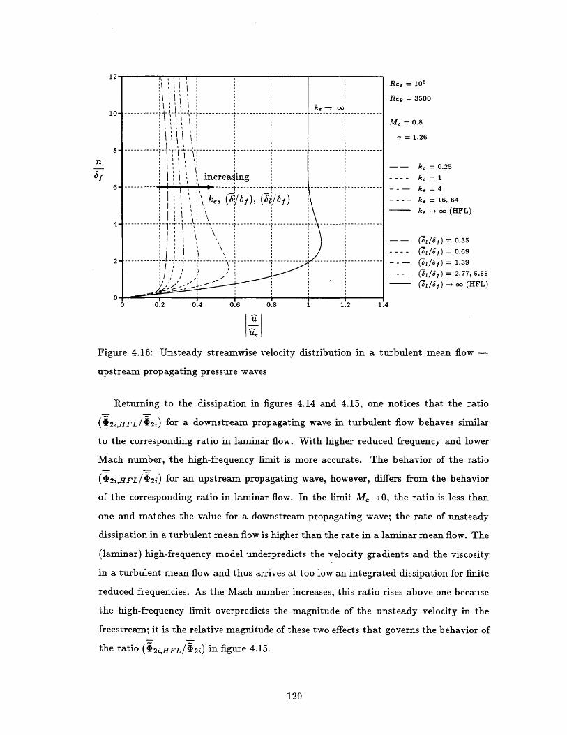
I
0
Ue
Figure 4.16: Unsteady streamwise velocity distribution in a turbulent mean flow -
upstream propagating pressure waves
Returning to the dissipation in figures 4.14 and 4.15, one notices that the ratio
(P2i,HFL/ 4 2i) for a downstream propagating wave in turbulent flow behaves similar
to the corresponding ratio in laminar flow. With higher reduced frequency and lower
Mach number, the high-frequency limit is more accurate. The behavior of the ratio
(42i,HFL/ 4 2i) for an upstream propagating wave, however, differs from the behavior
of the corresponding ratio in laminar flow. In the limit Me ->0, the ratio is less than
one and matches the value for a downstream propagating wave; the rate of unsteady
dissipation in a turbulent mean flow is higher than the rate in a laminar mean flow. The
(laminar) high-frequency model underpredicts the velocity gradients and the viscosity
in a turbulent mean flow and thus arrives at too low an integrated dissipation for finite
reduced frequencies. As the Mach number increases, this ratio rises above one because
the high-frequency limit overpredicts the magnitude of the unsteady velocity in the
freestream; it is the relative magnitude of these two effects that governs the behavior of
the ratio (4t2i,HFL/4 2) in figure 4.15.
120
Re, = 106
Ree = 3500
M, = 0.8
-y = 1.26
k, -- * 00I I
- ----------- - - -J ---------- I ----------- L----------------------- L-----------
increadingIL------I--- ----------- IL----------- ------------ L-----------
k,, (6/16f), (WI E6)
2 ------------ - -L -- -------- \-- ----------- ----------- ---------- -----------
8--
= 0.25
= 1
-4
=16, 64
-400 (HFL)
= 0.35
(it /f) = 0.69
(51/'f) = 1.39
(6;/6,) = 2.77, 5.55
(7L/vf) -+ oo (HFL)
I
n
6f
0.2 0.4 0.6 0.8 1 1.2 1.4
k,
ke
ke
ke

(/)= 0.35 0.69 1.39 2.77 5.55
Re. = 106
A Re = 3,500
0.5- ------- ----------- - ----------- - - --------------------
Me = 0.8
-y = . 2 6
0.4- ---------------------------- '- -------------- -------- ----------- -----------
0.41- ----------- --- - - ------- --------- --- -------- ------- -- ----------- -----------
7
k, -- + 0 (HFL) - ~020.3 ------------ - - - - - - - - - - - - - - - - - - - - - - - - - - , 0 2
k~4
16, 64
0 0.05 0.1 0.15 0.2 0.25 0.3 0.35 0.4
Ue
Figure 4.17: Unsteady streamwise velocity distribution near the wall in a turbulent
mean flow - upstream propagating pressure waves
It is puzzling, at first, that there is a (Mach-number dependent) range of reduced
frequencies in figure 4.15 for which the ratio (42i,HFL/2i) moves away from unity when
the reduced frequency is increased and moves back towards unity beyond that range.
This behavior can be explained with the help of figures 4.16 and 4.17. The major part
of the unsteady viscous dissipation occurs near the wall and is locally proportional to
the square of the velocity gradient and the viscosity. As a first approximation, the
integrated dissipation is set by the magnitude of the dissipation and the normal extent
over which it acts. On the normal scale (n/8f), the unsteady velocity gradient in figure
4.17 is steepest for low reduced frequencies, i.e for a laminar sublayer thickness much
less than the unsteady boundary layer thickness. It is steeper than the unsteady velocity
gradient in a laminar mean flow, the same way the steady velocity gradient is steeper
in a turbulent mean flow than in a laminar mean flow. As the reduced frequency is
increased, the ratio (Ti/5b) increases and the velocity gradient eventually equals the
one in the high-frequency limit and the turbulent viscosity approaches the laminar
121

viscosity. The high-frequency-limit solution is the same for all reduced frequencies on
the scales chosen for figure 4.17. This effect depends mainly on the ratio (6i/S) and
moves (42i,HFL/42i) towards higher values as the reduced frequency is increased; the
turbulent dissipation increases less rapidly than the dissipation predicted by the high-
reduced-frequency model. The change of behavior for higher reduced frequencies comes
about because of a second effect, seen in figure 4.16. When the reduced frequency is
sufficiently high, the maximum of the unsteady turbulent velocity approaches the value
predicted in the high-frequency limit before it veers off to match the boundary condition
in the freestream. Thus, the extent over which the gradient acts becomes larger and
(42i,HFL/ 2i) moves towards unity. This effect depends primarily on the Mach number
because it sets the freestream velocity disturbance via equation (4.46) and tends to
move the ratio of losses towards unity. For Me->O, this effect vanishes. Regardless of
the Mach number, the ratio (42i,HFL4 2i) always approaches unity for sufficiently high
reduced frequencies.
4.4 Unsteady Loss in the ACE Turbine Stage
The ACE turbine stage is a highly loaded, transonic high-pressure turbine stage, which
has been tested at MIT [50). A 2D-version of the rotor profile was investigated at
Oxford University [52, 54]. Its design is representative of modern high-pressure turbine
stages. A detailed computational account of the inviscid stator/rotor interaction is
presented in [6]; subsection 3.2.4 summarized the shock wave/blade row interaction. The
parameters in this simulation were similar to the parameters of subsection 3.2.4 except
that the code, UNSFLO, was run in the viscous mode [7], the rotor speed increased,
and the back pressure lowered slightly. The computational grid as well as the pressure
contours for the steady and the unsteady viscous simulation were shown in section 2.7.
Table 4.1 lists the input parameters. Lengths have been nondimensionalized by the
stator axial chord, the rotor speed by the inlet stagnation speed of sound, and the outlet
static pressure by the inlet stagnation pressure. The Reynolds number Re;,t is formed
with inlet stagnation quantities (upstream of the stator row) and the stator axial chord.
122

Rotor Axial Chord Ca,R 0.762
Stator Pitch PS 1.344
Rotor Pitch PR 0.778
Axial Gap 0.318
Inlet Flow Angle 00
Rotor Speed VR 0.737
Ratio of Specific Heats y 1.26
Outlet Static Pressure po 0.234
Stator suction surface x < 0.60 laminar
suction surface x > 0.65 turbulent
pressure surface x < 0.4 laminar
pressure surface x > 0.5 turbulent
Rotor Blades turbulent
Reynolds Number Rei,t = (pi,tai,tca,s/I;,t) 2.256 X 10⁶
Table 4.1: Input parameters for the ACE turbine stage simulation
The increased rotor speed in conjunction with the lower backpressure led to slightly
stronger trailing edge shock waves and reduced the mean rotor inflow angle from the
design inflow angle of 580 to 480, matching the experiments of Johnson et al. [54]. The
linear velocity analysis for this stage can be regarded as a viscous complement to the
investigation of Johnson et al., who studied the surface heat transfer fluctuations in
response to a passing shock wave.
In experiments by Ashworth et al. [52], the rotor boundary layer was found to be
laminar over most of the suction surface for low levels of freestream turbulence and in the
absence of wakes and shock waves. The pressure surface boundary layer was transitional.
Bar passing experiments, to simulate stator wakes and shock waves, showed that widely
spaced wakes and shock waves temporarily trip the boundary layer, which will relax
back to a laminar state after the disturbance has passed. For a bar spacing resembling
engine conditions, the boundary layer is transitional or turbulent. In the simulation,
the flow was prescribed to be turbulent from the rotor leading edge on. The turbulence
123

model was an algebraic model in the formulation of Cebeci and Smith [91]; all blades
were modeled as adiabatic blades.
4.4.1 Application of the Unsteady Viscous Loss Model
Predicted Loss
The loss model based on the near-wall approximation in the high-frequency limit, de-
scribed in section 4.1, was applied to the ACE turbine stage. The input required for the
model are the time-harmonics of the pressure gradient along the blade surfaces. These
may be the result of an inviscid or a viscous simulation, although the dominating effect
of the rotor passing through the oblique shock waves of the stator is captured inviscidly
10 AASR
12-
10- --- ---- ----------- ----------- ---------- ---------- ---------- ----------- -----------
leaiing edge: sR =
0.0
trailing edge: SR = 0.94 (pressure urface)
8------------------------------------ - ---- ------ ------ -----------sR =-1.6 (suction surface)
- ---------------- ---------- - ---------- --------- - ---------- ----------- -----------
rotor crown
4- ----------- ----------- ----------- -------- - -------- ---------- -----------
2------------------ ---------- ------ ------------- L---------- I----------- -----------
0 ---1.25 -1 -0.75 -0.5
rotor surface
-0.25 0
coordinate SR
0.25 0.5 0.75
Figure 4.18: Entropy rise per unit surface length on the ACE rotor
8In both cases, numerical smoothing will affect the unsteady pressure amplitudes.
See subsection 4.4.3 for details.
124

Figure 4.18 shows the distribution of the time-mean, mass-average entropy rise A9,
defined in equation (4.54), per unit surface length ASR along a rotor blade. A value
of SR=O corresponds to the rotor leading edge; positive and negative values correspond
to pressure and suction sides, respectively? The dissipation is concentrated on the suc-
tion surface between the rotor leading edge and the crown, where the pressure gradient
fluctuates in response to shock wave passing/reflection. Note that figure 2.14 shows
a pronounced rise of the (time-mean, mass-average) entropy in the rotor passage be-
tween the leading edge and the crown. The integrated entropy rise for a rotor blade is
A3= 2.8 x10⁻⁴, which is equivalent to a total pressure loss Ap = -1.3 x10- 3 . The above
numbers translate into an isentropic efficiency drop Az,,E/17s,E,D=-0.09%. Of the to-
tal, 70% is at the blade passing frequency and 16% in the second harmonic. Table 4.2
shows the contribution of individual harmonics to the entropy rise.
total entropy rise E Am'9 2.8 x 10- 4 1J100%
blade passing frequency 1.96 x 10- 4 70.1%
2 nd harmonic 0.45 x 10- 4 16.1%
3 rd harmonic 0.10 x 10⁻⁴ 3.6%
4 ,d harmonic 0.11 x 10⁻⁴ 4.0%
5 th harmonic 0.07 x 10⁻⁴ 2.5%
all higher harmonics 0.10 x 10⁻⁴ 3.7%
Table 4.2: Modal contributions to the Unsteady Viscous Loss of the ACE rotor
The Unsteady Viscous Loss on a stator was more than a factor of ten smaller than
the loss on a rotor; the stator passage is choked and the unsteady interaction between
shock waves and blade rows is much stronger in the rotor blade row.
Loss Model Errors
Figures 4.14 and 4.15 identified the parameters governing the error in the integrated
dissipation predicted by the high-frequency-limit model in turbulent flow. They are the
9 see figure 2.12
125

ratio of laminar sublayer thickness to unsteady boundary layer thickness, (6j/Sf), and
the freestream Mach number Me. These figures illustrated computations for a flow at
zero mean pressure gradient. Nevertheless, they can be used to estimate the error for the
ACE turbine stage, which has a strong favorable mean pressure gradient in the primary
region of Unsteady Viscous Loss. A mean pressure gradient enters through the wall
shear velocity u, in the definition of the laminar sublayer thickness (4.88). This defi-
nition is valid for arbitrary pressure gradients, Reynolds numbers, and Mach numbers.
Calculating the laminar sublayer thickness in the primary region of Unsteady Viscous
Loss from the wall shear of the steady simulation gives a thickness ratio of (6 l/65 )=1.2
for the unsteady boundary layer at the blade passing frequency. The freestream Mach
number in the primary loss region is Me~0.65 (in the rotor frame of reference). There-
fore, figure 4.14 suggests that the Unsteady Viscous Loss predicted for the ACE turbine
stage could be up to five times the nominal value of AT=2.8 x10- 4 . Figure 4.15 implies
that the loss model, when applied to the ACE turbine stage, overpredicts the actual
Unsteady Viscous Loss by no more than a factor of 1.5.
4.4.2 Efficiencies in the Numerical Simulation
The unsteady loss can also be inferred by comparing a steady and an unsteady viscous
simulation for the same profile. In a steady simulation, the stator outflow is averaged
at the interface to provide a spatially uniform and steady rotor inflow condition. The
efficiencies can be calculated from the time-mean, mass-average total pressures and
temperatures at the inlet boundary, the interface, and the outlet boundary. With the
total pressures and temperatures known, the isentropic efficiency may be calculated from
equation (2.49). Table 4.3 lists the isentropic efficiencies. Streamflux-average efficiencies
include the mixing loss from the dissipation of unsteady waves beyond the rotor outlet
boundary. The higher stage efficiency in the unsteady case is a direct consequence of
the mixing loss at the steady interface, as was discussed in section 2.7.
Detailed measurements of total temperature and total pressure with the spatial and
temporal resolution required to deduce the steady or the unsteady efficiency for this
126

stage are not available. Moreover, the experimental error bands would be of the same
order of magnitude as the numerical difference in efficiency between the steady and
the unsteady simulation. An indication that the calculated stage efficiency is realistic
can be obtained from a combined experimental and numerical study of a single stage
of comparable Reynolds number and total pressure ratio reported in [53]. While the
efficiencies are 2% to 3% less in [53], they include endwall loss, tip clearance loss, and
secondary flow loss, which are shown to add up to roughly one half of the total loss.
Table 4.3: Isent ropic efficiencies for the steady and the unsteady A( E simulation
The Unsteady Viscous Loss on the rotor blade surface is small compared to the total
loss in an unsteady viscous simulation. Nominally, i.e. at an isentropic efficiency drop of
(A77s,E/rs,E)=-0.9%, it accounts for only 1.43% of the total loss in the stage10 (or the
deviation of the stage efficiency from unity). Including the error bounds, it can account
for 1% to 7.1% of the total loss. The unsteady rotor efficiency is 1.25% less than the
steady rotor efficiency. The predicted Unsteady Viscous Loss could account for about
one third of this drop in the efficiency within the error bounds stated.
For an experiment that compared identical profiles in steady and in unsteady flow,
that is, in a linear cascade and in a stage, Hodson [9] reported an increase of 50% in
the rotor profile loss for the unsteady case. This was found to be due to the nature
of the boundary layer changing in sympathy with the passing of stator wakes. In the
simulation of the ACE turbine stage, the loss of the rotor blade row is 55% higher in
unsteady flow than in steady flow. Barring turbulence modeling, mechanisms that can
increase the loss in the unsteady simulation include unsteady shock waves [18], shock
t osee figure 2.14
127
[s,E steady unsteady
stage 93.58 % 94.06 %
stage (streamflux-averaged) 93.04 % 93.21 %
rotor 97.73 % 96.48 %
rotor (streamflux-averaged) 97.13 % 95.59 %

wave/boundary layer interaction, unsteady boundary layers, and numerical smoothing
in the freestream. In the steady as well as in the unsteady simulation, the boundary layer
was prescribed turbulent from the rotor leading edge on. Thus, there are no changes in
the transition point location or in the boundary layer character. The transition point on
the stator was also fixed. No separation, be it shock-induced or not, was found in either
simulation. While the magnitude of the loss increase in unsteady flow is in line with [9],the mechanism is different. Neither Unsteady Viscous Loss nor a change in the nature
of the boundary layer character can account for the loss increase in unsteady flow.
4.4.3 The Role of Numerical Smoothing
Questions remain about the exact magnitude of the Unsteady Viscous Loss. However,
they cannot explain the loss increase in unsteady flow, even if the errors of the loss model
are accounted for. The mechanisms behind the loss increase in the unsteady simulation
remain unclear, but there are indications that numerical smoothing in the freestream
plays an important role. Numerical smoothing, explicitly added to or implicit in a code,
is necessary to stabilize numerical simulations of the (inviscid) Euler equations. In
UNSFLO, the flow is governed by the Euler equations on the H-Grid through the blade
passages,' and by the Thin-Shear-Layer approximation of the Navier-Stokes equations in
the O-Grid around the blade surfaces. The H-grid roughly coincides with the freestream,
the core flow, while all blade boundary layers are contained within the O-grid. In the
O-grid, numerical smoothing is not necessary to stabilize the code; in fact, it would
corrupt the solution in the boundary layer.
Should numerical smoothing be an important player in the loss increase, there are
two implications. First, the simulation may not dissipate unsteady (pressure) waves pri-
marily in unsteady boundary layers, as happens in physical flowsl'but in the freestream.
Second, the unsteady pressure gradients acting on the blade surfaces, which are the in-
put to the loss model, may have been diminished prematurely, reducing the predicted
level of Unsteady Viscous Loss.
"Strictly speaking, it is not an H-grid because of the triangular cells at the inflow and outflow
boundaries. See figure 2.15.
1see introduction to chapter 4
128

The indications suggesting that numerical smoothing in the freestream plays an impor-
tant role in unsteady simulations are as follows:
First, it is difficult to detect more than three shock wave reflections in the visual-
ization of an unsteady simulation. To see whether such a small number is physically
realistic, the rate of amplitude attenuation due to dissipation in unsteady boundary lay-
ers and due to numerical smoothing in the freestream will be estimated and compared.
Second, in figure 2.14, the entropy rise between rotor crown and trailing edge is
steeper in the unsteady simulation. Neither the steady nor the unsteady simulation
showed any separation and the predicted Unsteady Viscous Loss is small in this region.
Third, the difference between the mass-average and the streamflux-average isentropic
rotor efficiency is about 0.6% in the steady case and 0.9% in the unsteady case. The
streamflux-average efficiency is less because it includes mixing losses downstream of the
rotor. The larger difference in the unsteady case is a consequence of the presence of
unsteadiness in the form of pressure waves, vorticity waves, and entropy waves at the
rotor exit. According to the inviscid simulations of subsection 3.2.4, the dissipation of
vorticity shed at the rotor trailing edge (Unsteady Circulation Loss) alone should have
accounted for a mixing loss of 0.3% in the isentropic efficiency.
The action of numerical smoothing in the freestream (the H-Grid) could explain these
observations. The following analytical and numerical considerations confirm that numer-
ical smoothing is the main mechanism leading to increased loss in unsteady simulations.
Attenuation of Pressure Waves at Boundaries
At the introduction to this chapter, it was shown that the energy associated with un-
steady waves is dissipated primarily in unsteady boundary layers. However, the rate at
which the wave amplitudes are attenuated remains to be determined. Based on the re-
sults of section 4.1, the attenuation of a pressure wave in laminar flow can be estimated.
Figure 4.19 illustrates the model problem graphically.
129

z
e 9 -
7 Z 7
Figure 4.19: Attenuation of an acoustic wave in an unsteady boundary layer
An incoming pressure wave at an angle of incidence 0 to the surface normal,
i; = 3 exp {i (k,s - kn - t)}, ( 4.90)
causes a reflected wave
i, = (1 - B) f exp {i (k,s + k.n - t) + i (} , (4.91)
where the amplitude attenuation factor , and the phase angle p depend on the complex
impedance R of the unsteady boundary layer which dissipates part of the wave energy.
R = Pr - (1 -3) e+ i ', (4.92)p
Recalling that bf < Af by (4.33), one can make the simplifying assumptions
kn6f < 1 (4.93)
and p < 1 (4.94)
at the edge of the unsteady boundary layer.
130
n
The incident as well as the reflected wave induce an unsteady streamwise velocity
distribution in the boundary layer. Due to inequalities (4.93) and (4.94), those are
nearly in phase. For an incompressible mean flow, the unsteady velocity gradient in the
boundary layer is approximately
--u~ (2 -,3) (1 - i) k,- R exp -1 - exp{i (k.s -t)} (4.95)n e) 2 I v/2- fI
from equation (4.44). The rate of dissipation per unit surface area in response to the
unsteady velocity gradient (4.95) is obtained from (4.53) as
(2 - 0)2 1 1 LP 242, = 2k s (4.96)
The average rate of acoustic energy incident per unit surface area is given by the acous-
tic intensity1 1
I; cosi ~ - ~- I2 Me C 056 , (4.97)
2 2
while the average rate of acoustic energy reflected per unit surface area is
1 1I, cos ~ (1 -3)2 |$, ~ - (1 - )2 I 2 Me cos G. (4.98)
2 2
The above acoustic intensities, strictly valid only for Me =0, are used for simplicity.
Since the objective is an order-of-magnitude argument, these simplification will not
compromise the subsequent conclusions; other consistent simplifications will be made.
Balancing incoming intensity, reflected intensity, and unsteady viscous dissipation, one
obtains
1 ~ ~ ~ k -- (e ) M o (2 -) (4.99)
Since 3 is small by definition, the solution of interest is found as
Me 2 tan0 sin0. (4.100)Re
The relation (k,/ke) 2 ~M2, obtained from equation (4.69) in the limit Me-0, has been
used in the above result. Alternatively, equation (4.100) can be expressed in the form
# = 2 tan 6 sin 0. (4.101)\ Re Af)
131
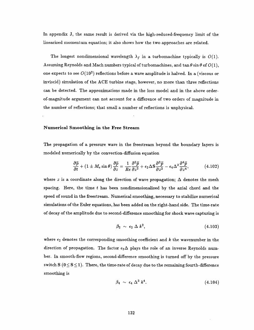
In appendix J, the same result is derived via the high-reduced-frequency limit of the
linearized momentum equation; it also shows how the two approaches are related.
The longest nondimensional wavelength A1 in a turbomachine typically is 0(1).
Assuming Reynolds and Mach numbers typical of turbomachines, and tan0 sin 0 of 0(1),
one expects to see 0(102) reflections before a wave amplitude is halved. In a (viscous or
inviscid) simulation of the ACE turbine stage, however, no more than three reflections
can be detected. The approximations made in the loss model and in the above order-
of-magnitude argument can not account for a difference of two orders of magnitude in
the number of reflections; that small a number of reflections is unphysical.
Numerical Smoothing in the Free Stream
The propagation of a pressure wave in the freestream beyond the boundary layers is
modeled numerically by the convection-diffusion equation
ap ap I a2- 192- 94-+ (1 Me sin6) - = --- +62AS -64A3 3(4.102)
t az Re i z 2 -z2 az (
where z is a coordinate along the direction of wave propagation; A denotes the mesh
spacing. Here, the time t has been nondimensionalized by the axial chord and the
speed of sound in the freestream. Numerical smoothing, necessary to stabilize numerical
simulations of the Euler equations, has been added on the right-hand side. The time-rate
of decay of the amplitude due to second-difference smoothing for shock wave capturing is
12 ~ 2 A k 2, (4.103)
where E2 denotes the corresponding smoothing coefficient and k the wavenumber in the
direction of propagation. The factor E2 A plays the role of an inverse Reynolds num-
ber. In smooth-flow regions, second-difference smoothing is turned off by the pressure
switch S (0 5 S <1). There, the time-rate of decay due to the remaining fourth-difference
smoothing is
#4 ~ E4 A3 k4 . (4.104)
132
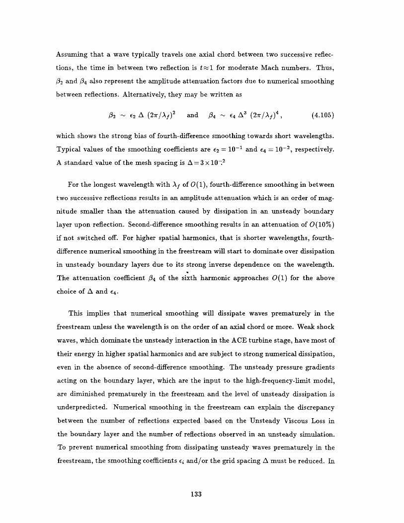
Assuming that a wave typically travels one axial chord between two successive reflec-
tions, the time in between two reflection is t~1 for moderate Mach numbers. Thus,
32 and 34 also represent the amplitude attenuation factors due to numerical smoothing
between reflections. Alternatively, they may be written as
32 ~ E 2 A (27r/Af) 2 and 84 ~ E4 A3 (27r/Af) 4 , (4.105)
which shows the strong bias of fourth-difference smoothing towards short wavelengths.
Typical values of the smoothing coefficients are E 2 = 10-1 and E4 = 10-2, respectively.
A standard value of the mesh spacing is A =3 x 10 2
For the longest wavelength with Af of 0(1), fourth-difference smoothing in between
two successive reflections results in an amplitude attenuation which is an order of mag-
nitude smaller than the attenuation caused by dissipation in an unsteady boundary
layer upon reflection. Second-difference smoothing results in an attenuation of 0(10%)
if not switched off. For higher spatial harmonics, that is shorter wavelengths, fourth-
difference numerical smoothing in the freestream will start to dominate over dissipation
in unsteady boundary layers due to its strong inverse dependence on the wavelength.
The attenuation coefficient 04 of the sixth harmonic approaches 0(1) for the above
choice of A and E4 .
This implies that numerical smoothing will dissipate waves prematurely in the
freestream unless the wavelength is on the order of an axial chord or more. Weak shock
waves, which dominate the unsteady interaction in the ACE turbine stage, have most of
their energy in higher spatial harmonics and are subject to strong numerical dissipation,
even in the absence of second-difference smoothing. The unsteady pressure gradients
acting on the boundary layer, which are the input to the high-frequency-limit model,
are diminished prematurely in the freestream and the level of unsteady dissipation is
underpredicted. Numerical smoothing in the freestream can explain the discrepancy
between the number of reflections expected based on the Unsteady Viscous Loss in
the boundary layer and the number of reflections observed in an unsteady simulation.
To prevent numerical smoothing from dissipating unsteady waves prematurely in the
freestream, the smoothing coefficients ei and/or the grid spacing A must be reduced. In
133

many CFD-codes, like the MacCormack method [64], numerical smoothing is implicit in
the formulation. Its level cannot be adjusted (other than increasing it by adding explicit
smoothing). In all formulations, a minimum level of smoothing is necessary to stabilize
the simulation. Thus, increasing the grid resolution, i.e reducing the grid spacing at the
expense of CPU-time, remains as the only viable solution in many applications.
4.4.4 Entropy Rise in the Simulation
Figure 4.20 shows the time-mean, mass-average entropy, defined in equation (2.58), in
the freestream of the rotor passage; both the steady and the unsteady viscous simulation
are shown. For simplicity, the freestream was assumed to coincide with the H-grid in the
rotor passage. While the freestream extends into the O-grid around the rotor blades, it
is only the flow on the H-grid that is subject to numerical smoothing.
0.0155-
0.0145-
0.0135-
H-gridentropy -9
0.0125
0.0115-
0.0105-
0.00951.
rotor crown:----------- ----------- ----------- -- -------- ----------- ----------- ----------- ------- --
-- ----- --- - -- -- --- ---- --- - --- -- --- --- -- -- -- -- -- - --- --- -- -- --- -- -- -- -- -- --- ---- -- --- -
rotor leading edge
----------- ----------- ----------- ----------- ---- ------ ----------- -------
----------------- ----------- ----------- ----------- ----------- ----------- ------- ----
rotor trailinig edge
3 1.4 1.5 1.6 1.7 1.8 1.9
- - - steadyaxial location z - - steady
unsteady
2 2.1
Figure 4.20: Average entropy in the rotor passage H-grid (the freestream)
134

The entropy rise between the rotor leading edge and the rotor trailing edge in the
unsteady simulation is about three times as large as in the steady simulation. Clearly,
the locus of loss increase in the unsteady simulation is in the freestream, with the
primary mechanism being numerical smoothing.
Both figure 2.14 and figure 4.20 show regions in which the average entropy is axially
decreasing. The decrease happens in the freestream (on the H-grid), as is seen from
figure 4.20. In figure 2.14, the decrease is masked by the monotonically rising average
entropy in the boundary layer contained in the O-grid. While it is not clear what
mechanism causes the decrease in average entropy, it is a numerical artifact most likely
linked to numerical smoothing. By its very nature, numerical smoothing mixes out the
flow. In uniform mean flow, a control-volume argument as presented in chapter 2 can
be used to calculate the associated entropy rise. Moreover, the entropy is guaranteed
to rise monotonically in the axial direction. Second-difference smoothing mimics the
action of the physical viscosity; fourth-difference smoothing has no physical counterpart
in real flows. The control-volume argument allows no conclusion about the path a fluid
particle's entropy takes in an unsteady nonuniform flow subject to fourth-difference
numerical smoothing.
The entropy rise in the freestream cannot be discounted as a numerical artifact
without physical implication. The argument was made in detail in section 2.4. While
the mechanisms and the locus of unsteady loss differ in numerical simulations and real
physical flows, the entropy rise in the freestream of a numerical simulation, and the
associated loss, are possibly indicative of the level of Unsteady Viscous Loss that would
be seen in the boundary layer in the absence of numerical smoothing. As was pointed
out in section 2.4, the entropy rise associated with the dissipation of unsteady waves
does not depend on the mechanism of dissipation. While numerical smoothing shifts
the locus of dissipation into the freestream, the associated entropy rise is expected to
be approximately correct. The statement is not an unqualified one because the entropy
rise still depends on the mean flow state at the locus of dissipation.
135

rotOr crown
0.032 ----------- ----------- ----------- -- ------- ----------- ----------- ----------- ---- ------
0.028- ----------- ----------- ----------- -- -------- -------- --------- ----------- --- ------
0-grid rotor leading edgeentropy s
0.024- - --------- ----------- ---------- -- ---------L ---------- ----------- -_ - ----- --------
0.016- ------------------------- -----
0.016 - ------ - ----------- ---------- ----------- ----------- ----------- ----------- ------- ----
rotor trailing edge
0.0121.3 1.4 1.5 1.6 1.7 1.8 1.9 2 2.1
- - - steadyaxial location x_ unsteady
Figure 4.21: Average entropy in the O-grid (boundary layers) around the rotor blades
Figure 4.21 shows the average entropy in the 0-grid. In the steady simulation,
the mass-average entropy at the leading edge only slightly exceeds the uniform entropy
level after mixing at the interface. Surprisingly, the time-mean mass-average entropy
at the leading edge is higher in the unsteady simulation, but rises more slowly. As a
consequence of the predicted Unsteady Viscous Loss, one would expect to see a steeper
rise between leading edge and rotor crown in the unsteady simulation. At their nominal
level, Unsteady Viscous Loss causes a rise of AT = 2.8 x 10- based on the time-mean
axial mass-flux through a rotor passage. The Unsteady Viscous Loss, however, happens
locally near the rotor blade surface. Based on the mass-flux in the O-grid, the average
entropy rise is O(10-3), nominally. On the entropy scale of figure 4.21, an entropy rise
of O(10-3) is still small. The major problem in interpreting figure 4.21 is the fact that
the boundary between 0-grid and H-grid is not a streamline. Thus, fluid is entrained in
or passes out of the O-grid. The associated change in the average entropy of the O-grid
masks any entropy rise due to Unsteady Viscous Loss. Without computing streamlines,
it is not possible to separate the effects of entrainment and Unsteady Viscous Loss.
136

The blade surface itself is a streamline. Thus, a surface entropy plot does not
suffer from entrainment effects. Figure 4.22 shows the time-mean entropy on the rotor
surface. In the unsteady case, the mean entropy rises faster along the front portion
of the suction surface, which could be attributed to Unsteady Viscous Loss. While
the Unsteady Viscous Loss occurs in the near-wall region, the exact magnitude of the
associated rise in the surface entropy is not known. It is not possible to determine
whether the difference between the steady and the unsteady entropy rise corresponds
to the generation of Unsteady Viscous Loss. On the pressure surface, there is an almost
constant offset between the entropy in the steady and the unsteady case. Its magnitude
roughly matches the entropy rise due to the mixing loss at the steady interface.
0.18rotor crown
0.15- ---------- - ---- -- - - -------- --------- - --- ---
rotor leading edgesurface
entropy s-0.09- ------ -- ----- - - ---------- ---------- - --------- --------- - --- --- -
suytion surfayepressure surface
0.03- -- - ----------- ----------- ----------- ----------- ----- --- ------ -------- --0.0 ~ --- -- -------
rotor trailing edge
1.3 1.4 1.5 1.6 1.7 1.8 1.9 2 2.1
- - - steadyaxial location x unsteady
Figure 4.22: Time-mean rotor surface entropy
While Unsteady Viscous Loss could be one explanation for the difference between
steady and unsteady surface entropy, it could also be due to the migration of stator
wake fluid to the suction surface. Due to its velocity defect in the stator frame, the
wake has a slip velocity perpendicular to the freestream in the rotor frame. Wake fluid
137

of higher entropy piles up on the suction side, while freestream fluid with lower entropy
drifts to the pressure side.
4.5 Summary - Unsteady Viscous Loss
Based on a near-wall approximation in the high-reduced-frequency limit, a model for the
Unsteady Viscous Loss with a non-zero time-mean has been formulated. The loss is due
to dissipation in unsteady boundary layers driven by unsteady pressure gradients. The
errors introduced into the loss model by a departure from the high-reduced frequency
limit have been examined in laminar and turbulent mean flows; at high freestream Mach
numbers in turbulent flow, they can be appreciable.
The loss model was applied to the ACE turbine stage, which exhibits strong inter-
action between oblique shock waves and the rotor blade row. The Unsteady Viscous
Loss was found to be small. Nominally, i.e. without taking the loss model errors into
consideration, they account for only 1.4% of the total loss in an unsteady simulation
of the flow through the stage. The error band for this case is significant, allowing for
an Unsteady Viscous Loss up to five times the nominal level. At that level, Unsteady
Viscous Loss would be of the same magnitude as the Unsteady Circulation Loss. While
still small compared to the total loss of an unsteady simulation, it could account for a
third of the unsteady loss increase in the rotor passage. The ACE turbine stage is repre-
sentative of current high-pressure turbine designs but its level of unsteadiness is at the
upper end of the range found in turbomachinery. Generally, the level of unsteadiness,
and the associated Unsteady Viscous Loss, are lower.
The loss in the rotor passage is 55% higher in the unsteady simulation than in the
steady simulation. Neither the Unsteady Viscous Loss nor a change in the boundary
layer character account for the magnitude of the loss increase. The dominant mecha-
nism of loss increase was found to be numerical smoothing in the freestream. Numerical
simulations damp unsteady waves by way of numerical smoothing in the freestream,
138

and not in unsteady boundary layers, as do real flows. As a consequence, the computed
pressure gradients, which drive the model for the Unsteady Viscous Loss, can be dimin-
ished prematurely, reducing the predicted loss. While the loss increase in unsteady flow
occurs in the wrong location, its level is possibly indicative of the Unsteady Viscous Loss
that would otherwise be seen in the boundary layer. To prevent numerical smoothing
from dominating, the level of numerical smoothing in simulations must be decreased. If
numerical smoothing is implicit to a code, its smoothing coefficients cannot be adjusted
and the grid spacing needs to be reduced.
In the simulation, it proved difficult to separate the effect of Unsteady Viscous
Loss from the effects of other phenomena, in particular in the presence of numerical
smoothing. At its small (nominal) magnitude, it is easily masked. The uncertainty
about its exact magnitude averaged over the blade passage or the boundary layer,
and lack of knowledge about its effect on the surface entropy further complicate the
identification of Unsteady Viscous Loss in the simulation.
139

Chapter 5
Concluding Remarks
This thesis reports an analytical and numerical investigation of the second-order effects
of unsteadiness on the efficiency of turbomachines, using linear, two-dimensional models.
The main themes of the thesis are the identification of the physical nature and the
location of unsteady loss mechanisms, the magnitude of the associated losses and their
effect on the time-mean efficiency, and the assessment of the modeling accuracy of
numerical simulations with respect to unsteady losses.
5.1 Summary
The thesis research consisted of three distinct parts, corresponding to chapters 2, 3,
and 4. The scope and the results for each chapter are briefly summarized below.
5.1.1 Chapter 2 - Unsteadiness and Loss
Chapter 2 established, for the first time in a rigorous mathematical manner, a link be-
tween the dissipation (mixing out) of unsteadiness in a compressible flow in two dimen-
sions and the efficiency of a turbomachine. A novel approach, involving an asymptotic
analysis and a control-volume argument for a flow governed by the linearized Euler
equations, related the dissipation of an arbitrary combination of unsteady waves in a
uniform mean flow to an entropy rise. The entropy rise was in turn related to a change
in the turbomachine performance through a linearization of the isentropic efficiency.
140

The unsteady waves permitted in an inviscid, compressible, linearized flow in two
dimensions are convected entropy and vorticity waves and propagating, or evanescent,
pressure waves. In an unsteady nonuniform flow, the time-mean of the flux-average
entropy is the only loss measure with a sound physical foundation. The separate con-
tributions to the second-order entropy rise (upon dissipation) from waves of different
frequency, wave number, and physical nature were explained. It was proved that contri-
butions from waves of different physical nature do not crosscouple and that evanescent
pressure waves do not contribute to the mixing loss.
The dependence of the accuracy of the predicted entropy rise on the wave amplitudes
was investigated by comparison to the numerically determined (nonlinear) entropy rise.
The loss model was employed for the first analysis of mixing loss at the stator/rotor
interface of a steady simulation. At the interface, the nonuniform stator outflow is
averaged to provide steady, uniform rotor inflow conditions. For the case examined, a
viscous simulation of a high-pressure turbine stage called the ACE turbine stage, the
mixing loss accounted for about 20% of the stage entropy rise in the steady simulation.
The linear model identified the contributions from pressure waves, vorticity waves, and
entropy waves to the mixing loss. The agreement between the predicted mixing loss and
the (nonlinear) mixing loss observed in the steady simulation was excellent, despite the
large magnitude of the perturbations in the stator outflow. It was pointed out that, as
a consequence of the averaging at the stator/rotor interface, the steady simulation of
a stage can have a lower efficiency than the corresponding unsteady simulation. This
aspect of steady simulations seems to have gone unrecognized, so far.
It is also relevant to note that Mathematica®, a software package for performing
symbolic mathematical manipulations by computer, proved to be an extremely useful
tool in carrying out the extensive manipulations required by the asymptotic analysis.
141

5.1.2 Chapters 3 and 4 - Unsteady Loss Mechanisms
The thesis treated two unsteady loss mechanisms in a 2D, linearized framework. They
are called Unsteady Circulation Loss and Unsteady Viscous Loss, respectively.
Chapter 3 - Unsteady Circulation Loss
Unsteady Circulation Loss results from the transfer of mean-flow energy to kinetic
energy associated with vorticity shed at the trailing edges of a blade row. In accordance
with Kelvin's Circulation Theorem, the vorticity is shed in response to a time-varying
blade circulation. The kinetic energy associated with the shed vorticity is unlikely to
be recovered and is thus related to an efficiency drop as detailed in chapter 2.
While Unsteady Circulation Loss has been considered previously, this thesis pre-
sented the first application of numerical simulations to the loss mechanism. The use
of circulation amplitudes determined from simulations allows one to obtain Unsteady
Circulation Losses for arbitrary blade and/or stage geometries and Mach numbers.
Eliminating the need to estimate the circulation amplitudes or to deduce them from
thin-airfoil theory results in a realistic loss measure for modern turbomachines.
The Unsteady Circulation Losses were found to be small. For the case with the
strongest unsteady interaction between blade rows, the ACE turbine stage, Unsteady
Circulation Loss led to a drop in the isentropic stage efficiency of only 0.3%.
The most important interaction mechanisms leading to an unsteady circulation were
found to be wake/blade row interaction and oblique shock wave/blade row interaction.
Potential interaction played a minor role only. In the so-called NASA-stage 67 com-
pressor, for example, Unsteady Circulation Loss led to a drop in the efficiency of only
0.03% for the smallest gap between blade rows.
The circulation amplitudes were found to be surprisingly small, i.e. 0(1%) of the
time-mean circulation. Even the ACE turbine stage with a 40% peak-to-peak variation
142

in the rotor lift, only showed a peak-to-peak variation in the rotor circulation of 5.5%.
No further work is required on the subject of Unsteady Circulation Loss because its
magnitude has been clearly established and was found to be small.
Chapter 4 - Unsteady Viscous Loss
The unsteady stator/rotor interaction can generate strong pressure waves. Unsteady
Viscous Loss is a consequence of dissipation in unsteady boundary layers driven by
these pressure waves. The proposed loss model represents the first attempt to model
Unsteady Viscous Loss.
A high-reduced-frequency limit was used to obtain the streamwise velocity distribu-
tion in the laminar Stokes sublayer driven by unsteady pressure gradients. The driving
pressure gradients were obtained from a simulation. In the high-frequency limit, the
dissipation in unsteady boundary layers depends only on the unsteady shear. The as-
sociated entropy rise was again related to a drop in the isentropic efficiency.
To check the errors introduced by a departure from the high-reduced-frequency
limit, a numerical study was performed on a flat plate boundary layer subject to a
pressure wave disturbance. The accuracy of the predicted dissipation was shown to
depend primarily on the freestream Mach number and the ratio of the laminar sublayer
thickness (of the turbulent mean flow) to the unsteady boundary layer thickness.
The loss model was applied to the ACE-turbine stage. Unsteady Viscous Loss was
predicted to cause a drop in the isentropic stage efficiency of 0.09%. Compared to
the total loss in an unsteady viscous simulation, this is a very small contribution; it
accounts for only 1.4% of the total loss. Taking into account errors due to modeling
approximations, the loss could be at most five times the predicted level. At that level, it
would be roughly of the same magnitude as the Unsteady Circulation Loss but remain
a small contribution, accounting for no more than 7.1% of the total loss.
143

Unsteady Viscous Loss could, however, account for about one third of the loss in-
crease in the rotor passage observed in the unsteady simulation over the level in the
corresponding steady simulation. Analytical considerations and detailed examination of
the simulations showed that the increase is induced primarily by numerical smoothing.
Numerical smoothing shifts the primary locus of unsteady loss from boundary layers into
the freestream. Pressure waves, which constitute the input to the loss model, are atten-
uated prematurely in the freestream, reducing the predicted level of Unsteady Viscous
Loss. The magnitude of the loss increase in the freestream of the unsteady simulation is
possibly indicative of the levels of Unsteady Viscous Loss that would otherwise appear
in unsteady boundary layers.
The thesis contains the first investigation on the origin of the increase in loss seen in-
the rotor passage of an unsteady viscous simulation. The finding that there can be differ-
ent unsteady loss mechanisms and loci in physical flows and simulations, is an important
one. Since unsteady simulations are used to assess the performance of turbomachinery,
the potential problems and the limitations of CFD-codes need to be understood.
In contrast to Unsteady Circulation Loss, Unsteady Viscous Loss requires future
work to address the problems identified in the course of this thesis.
Synopsis of Unsteady Loss
The contributions of the unsteady loss mechanisms considered to the overall loss in a
stage with a high level of unsteadiness are small, but not negligible if an accurate account
of the loss sources and the time-mean efficiency are required. This is particularly true as
long as the magnitude of Unsteady Viscous Loss cannot be established more accurately.
As discussed above, Unsteady Viscous Loss could be a significant contributor to
unsteady loss. A less conditional statement must await additional research into the
effect of numerical smoothing and modeling approximations on the predicted level of
Unsteady Viscous Loss.
144

5.2 Future Work Recommendations
5.2.1 Chapter 2 - Unsteadiness and Loss
Chapter 2 linked unsteady waves to the entropy rise upon their dissipation. While it was
concluded that little of the energy associated with unsteady waves can be recovered, a
closer analytical study of rectification mechanisms in turbomachines and a quantitative
measure of rectification would be highly desirable.
References on wave reflection and transmission through blade rows did not provide
a clear picture on reflection and transmission coefficients. The coefficients vary greatly,
depending on the exact choice of parameters like Mach number, incidence angle, and
stagger angle. None of the references treated geometries realistic for turbomachinery.
Therefore, it was difficult to make a general conclusion about the relative importance
of transmission versus reflection, and ultimately about the locus of dissipation.
If an unsteady wave is not dissipated 'in place', but only after transmission through
blade rows, it may extract additional energy from the mean flow. Also, if dissipation of
unsteady waves happens in a nonuniform mean flow, the associated loss is not known.
The asymptotic analysis for a control volume holds only in a uniform mean flow. Both
of the above issues should be addressed analytically.
An experiment, measuring the unsteady flow field of a turbine stage with the spatial
and temporal resolution required to identify the unsteady waves, could provide answers
to the above questions. Knowing the wave content at the stator/rotor interface and the
outflow boundary would allow one to draw a conclusion about the relative importance
of reflection versus transmission and the locus of dissipation.
145

5.2.2 Chapter 4 - Unsteady Viscous Loss
Chapter 4 treated Unsteady Viscous Loss and applied the loss model to the ACE turbine
stage. The predicted loss was small, but its magnitude was not well-defined due to
modeling approximations and the action of numerical smoothing.
Numerical smoothing was found to shift the primary locus of unsteady loss in nu-
merical simulations from boundary layers into the freestream. While loss mechanisms
and locations differ in physical flows and numerical simulations, the entropy rise in the
freestream is possibly indicative of the level of Unsteady Viscous Loss in physical flows.
Therefore, the first step in any future work should be an analytical assessment of the
consequences stemming from differing mechanisms and locations of unsteady loss if the
predicted level of unsteady loss is realistic.
Since numerical smoothing is necessary to stabilize CFD-codes, and in many cases
is implicit in the numerical method, the only way to reduce nonphysical losses in the
freestream is to increase the grid resolution at the expense of CPU-time. Careful bench-
mark calculations with high grid resolution are recommended to establish the resolution
required to have identical dissipation mechanism in simulated and real flows.
Experiments focusing on the unsteady pressure gradients on the blade surfaces are
suggested; these could be used for two purposes. First, they could be compared to
pressure gradients obtained in a numerical simulation to give some guidance as to when
the dissipation mechanism in a simulation is physically realistic. Second, the data could
be used as an alternate source of input to a loss model.
Once the input, i.e. the unsteady pressure gradients, can be trusted, an improved
loss model should be developed. In the present formulation, the errors in the predicted
dissipation are appreciable when the model is applied to turbomachinery flows of prac-
tical interest. A model like the one used for the numerical error evaluation could be
employed to account for turbulent mean flows and mean-flow convection.
146

Bibliography
[1] D.R. Lindquist. Computation of Unsteady Transonic Flowfields Using Shock Cap-turing and the Linear Perturbation Euler Equations. Ph.D. Thesis, MassachusettsInstitute of Technology, Dezember 1991.
[2] K.C. Hall. A Linearized Euler Analysis of Unsteady Flow in Turbomachinery.Ph.D. Thesis, Massachusetts Institute of Technology, 1987.
[3] J.J. Adamzcyk. Model Equations for Simulating Flows in Multistage Turbomachin-ery. ASME Paper 85-GT-226, 1985.
[4] M.B. Giles. A Framework for Multi-Stage Unsteady Flow Calculations. Confer-ence proceedings of the 6 th International Symposium on Unsteady Aerodynamics,Aeroacoustics, and Aeroelasticity of Turbomachines and Propellers, University ofNotre Dame, 1991.
[5] M.B. Giles. Calculations of Unsteady Wake/Rotor Interactions. Journal of Propul-sion and Power 4(4), 1988.
[6] M.B. Giles. Stator/Rotor Interaction in a Transonic Turbine. Journal of Propulsionand Power 6(5), 1990.
[7] M.B. Giles and R. Haimes. Validation of a Numerical Method for Unsteady FlowCalculations. ASME Paper 91-GT-271, 1991.
[8] M.B. Giles and R. Haimes. Advanced Interactive Visualization For CFD. Comput-ing Systems in Engineering 1(1), 1990.
[9] H.P. Hodson. Boundary Layer and Loss Measurements on the Rotor of an Axial-Flow Turbine. ASME Paper 83-GT-4, 1983.
[10] C. Keller. Energy Losses on High-Speed Turbomachines Resulting from IrregularFlow to the Runner Wheel. Escher-Wyss News, March/April 1935.
[11] N.H. Kemp and W.R. Sears. On the Wake Energy of Moving Cascades. Journal ofApplied Mechanics 23, June 1956.
[12] Th. von Karman and W.R. Sears. Airfoil Theory for Non- Uniform Motion. Journalof the Aeronautical Sciences 5, August 1938.
[13] W.R. Sears. Some Aspects of Non-Stationary Airfoil Theory and Its Practical Ap-plications. Journal of the Aeronautical Sciences 8, January 1941.
[14] N.H. Kemp and W.R. Sears. On the Lift and Circulation of Airfoils in SomeUnsteady-Flow Problems. Journal of Aeronautical Sciences 19, October 1952.
147

[15] N.H. Kemp and W.R. Sears. Aerodynamic Interference Between Moving BladeRows. Journal of the Aeronautical Sciences 20, September 1953.
[16] W.R. Hawthorne. Flow Through Moving Cascades of Lifting Lines with FluctuatingLift. Journal of Mechanical Engineering Science 15(1), 1973.
[17] J.L. Kerrebrock and A.A. Mikolajczak. Intra-Stator Transport of Rotor Wakes andIts Effect on Compressor Performance. Journal of Engineering for Power, 1970.
[18] W.F. Ng, A.H. Epstein. Unsteady Losses in Transonic Compressors. Journal ofEngineering for Power 107(2), 1985.
[19] A.J. Strazisar Investigation of Flow Phenomena in a Transonic Rotor Using a LaserAnemometer. Journal of Engineering for Power 107(2), 1985.
[20] M.D. Hathaway, J.Gertz, A. Epstein, and A.J. Strazisar. Rotor Wake Characteris-tics of a Transonic Axial Flow Fan. AIAA Paper 85-1133, 1985.
[21] P.R. Owen. Computational Simulation of Unsteady Flow in a Transonic Compres-sor Rotor. MIT S.M.-Thesis, 1986.
[22] L.H. Smith. Casing Boundary Layers in Multistage Axial Flow Compressors. FlowResearch in Blading, edited by L.S. Dzung, Elsevier Publishing Company, Amster-dam, 1970.
[23] A.A. Mikolajczak. The Practical Importance of Unsteady Flow. AGARD-CP 177.
[24] R. Hetherington and R.R. Moritz. The Influence of Unsteady Flow Phenomena onDesign and Operation of Aero Engines. AGARD-CP 177.
[25] A.O. Lopatitskii et al. Energy Losses in the Transient State of an Incident Flowon the Moving Blades of Turbine Stages. Energomashinostroenie 15, 1969.
[26] I.Y. Kirillov, A.S. Laskin and C.G. Shpenzer Influence of Unsteadiness of the Flowon Efficiency of Turbine Stages. Teploenergetika 17(10), 1970.
[27] V.Y. Yurinskiy and I. Shestachenko. Losses in an Impulse Turbine Cascade in anUnsteady Flow. Fluid Mechanics-Soviet Research 3(1), 1974.
[28] H.J. Obremski and A.A. Feier. Transition in Oscillatory Boundary Layer Flows.Journal of Fluid Mechanics 29(1), 1967.
[29] G.J. Walker. The Unsteady Nature of Boundary Layer Transition on an Axial-FlowCompressor Blade. ASME Paper 74-GT-135, 1974.
[30] H. Pfeil, R. Herbst. Transition Process of Instationary Boundary Layers. ASMEPaper 79-GT-128, 1979.
[31] H. Pfeil, R. Herbst and T. Schr6der. Investigation of the Laminar- Turbulent Tran-sition of Boundary Layers Disturbed by Wakes. ASME Paper 82-GT-124, 1982.
[32] R.L. Evans. Boundary Layer Development on an Axial-Flow Compressor StatorBlade. Journal of Engineering for Power 100, 1978.
148

[33] R.P. Dring, H.D. Joslyn, L.W. Hardin, J.H. Wayner. Turbine Rotor-Stator Inter-action. ASME Paper 82-GT-3, 1982.
[34] H.P. Hodson. Modeling Unsteady Transition and Its Effect on Profile Loss.AGARD-CP-468.
[35] J.D. Doorly and M.L.G. Oldfield. Simulation of the Effects of Shock-Wave Pass-ing on a Turbine Rotor Blade. Journal of Engineering for Gas Turbines andPower 107(4), 1985.
[36] D.S. Whitehead. The Calculation of Steady and Unsteady Transonic Flow in Cas-cades. University of Cambridge, Department of Engineering Report CUED/A-Turbo/TR 118, 1982.
[37] J.M. Verdon and J.R. Caspar. A Linearized Unsteady Aerodynamic Analysis forTransonic Cascades. Journal of Fluid Mechanics 149, 1984.
[38] R.H. Ni and F. Sisto. Numerical Computations of Non-Stationary Aerodynamics ofFlat Plate Cascades in Compressible Flow. ASME Paper 75-GT-5, 1975.
[39] R.H. Ni. A Multiple-Grid Scheme for Solving the Euler-Equations. AIAA Jour-nal 20(11).
[40] R.H. Ni and J.C. Bogoian. Prediction of 3D Multistage Turbine Flow Fields Usinga Multiple-Grid Euler Solver. AIAA Paper 89-0203, 1989.
[41] M.M. Rai. A Relaxation Approach to Patched-Grid Calculations with the EulerEquations. Journal of Computational Physics 66(1), 1986.
[42] H.P. Hodson. An Inviscid Blade-to-Blade Prediction of a Wake-Generated UnsteadyFlow. ASME Paper 84-GT-43, 1984.
[43] J.D. Denton. An Improved Time-Marching Method for Turbomachinery Flow Cal-
culations. ASME Paper 82-GT-239, 1982.
[44] M.M. Rai. Navier-Stokes Simulations of Rotor-Stator Interaction Using Patchedand Overlaid Grids. ASME Paper 85-1519, 1985.
[45] J.D. Doorly and M.L.G. Oldfield. Simulation of Wake-Passing in a StationaryTurbine Rotor Cascade. Journal of Propulsion and Power 1(4), 1985.
[46] T.L. Butler, O.P. Sharma, H.D. Joslyn and R.P. Dring. Inlet Temperature Distor-tion in an Axial Flow Turbine Stage. AIAA Paper 86-1468, 1986.
[47] B. Krouthen. Numerical Investigation of Hot Streaks in Turbines. MIT, Computa-tional Fluid Dynamics Lab, CFDL-TR-88-9, 1988.
[48] R.H. Ni and R. Takahashi. Hot Streak Migration Through a Turbine Stage - AnUnsteady Flow Simulation. NASA-MSFC CFD-workshop.
[49] M.M. Rai and R.P. Dring. Navier-Stokes Analysis of Redistribution of Inlet Tem-perature Profiles in a Turbine. AIAA Paper 87-2146, 1987.
149

[50] G.R. Guenette, A.H. Epstein, M.B. Giles, R. Haimes, and R.J.G. Norton. FullyScaled Transonic Turbine Rotor Heat Transfer Measurements.ASME Paper 88-GT-171, 1988.
[51] R.S. Abhari, G.R. Guenette, A.H. Epstein, and M.B. Giles. Comparison of Time-Resolved Turbine Rotor Blade Heat Transfer Measurements and Numerical Calcu-lations. ASME Paper 91-GT-268, 1991.
[52] D.A. Ashworth, J.E. LaGraff, D.L. Schultz, and K.J. Grindrot. Unsteady Aero-dynamic and Heat Transfer Processes in a Transonic Turbine Stage. Journal ofEngineering for Gas Turbine and Power 107, 1985.
[53] R.J. Boyle, J.E. Haas, and T. Katsanis. Predicted Turbine Stage Performance UsingQuasi- Three-Dimensional and Boundary-Layer A nalysis. Journal of Propulsion andPower 1(3), 1985. York, 1974.
[54] A.B. Johnson, M.J. Rigby, M.L.G. Oldfield, R.W. Ainsworth, and M.J. Oliver.Surface Heat Transfer Fluctuations on a Turbine Rotor Blade due to UpstreamShock Wave Passing. ASME Paper 88-GT-172, 1988.
[55] M.B. Giles. Non-Reflecting Boundary Conditions for the Euler Equations. MIT-CFDL-Report, CFDL-TR-88-1, February 1988.
[56] R.K. Amiet. Transmission and Reflection of Sound by Two Blade Rows. Journalof Sound and Vibrations 34(3), 1974.
[57] S. Kaji and T. Okazaki. Propagation of Sound Waves Through a Blade Row. Part I:Analysis Based on the Semi-Actuator Disk Theory. Journal of Sound and Vibra-tions 11(3), 1970.
[58] S. Kaji and T. Okazaki. Propagation of Sound Waves Through a Blade Row. Part II:Analysis Based on the Acceleration Potential Method. Journal of Sound and Vibra-tions 11(3), 1970.
[59] R.S. Muir. The Application of a Semi-Actuator Disk Model to Sound TransmissionCalculations in Turbomachinery, Part I:The Single Blade Row. Journal of Soundand Vibrations 54(3), 1977.
[60] P.J. Grooth Wave Reflection by a Flat Plate Cascade. Master's Thesis, Mas-sachusetts Institute of Technology, September 1990.
[61] P.E. Doak. Momentum Potential Theory of Energy Flux Carried by MomentumFluctuations. Journal of Sound and Vibrations 131(1), 1989.
[62] O.S. Ryshov and G.M. Shefter. On the Energy of Acoustic Waves Propagating ina Moving Media. Journal of Applied Mathematics and Mechanics 26, 1962.
[63] W. Eversman. Acoustic Energy in Ducts:Further Observations. Journal of Soundand Vibrations 62(4), 1979.
[64] R.W. McCormack A Numerical Method for Solving the Equations of CompressibleViscous Flow. AIAA Paper 81-0110, 1981.
150
[65] L. N. Cattafesta. An Experimental Investigation of the Effects of Inlet Radial Tem-perature Profiles on the Aerodynamic Performance of a Transonic Turbine Stage.Master's Thesis, Massachusetts Institute of Technology, August 1988.
[66] C.F. Gerald and P.O. Wheatley Applied Numerical Analysis, 3rd edition, chapter 4.Addison-Wesley Publishing Company, 1984.
[67] M.B. Giles. UNSFLO: A Numerical Method for Calculating Unsteady Stator/Rotor
Interaction. Technical Report TR-86-6, MIT Computational Fluid Dynamics Lab-
oratory, October 1988.
[68] J.D. Denton. The Calculation of Three-Dimensional Viscous Flow Through Multi-
stage Turbomachines ASME Paper 90-GT-19, 1990.
[69] H.P. Hodson. Measurements of Wake-Generated Unsteadiness in the Rotor Pas-
sages of Axial Flow Turbines. ASME Paper 84-GT-189, 1984.
[70] N.H. Kemp and W.R. Sears. The Unsteady Forces Due to Viscous Wakes in Tur-bomachines. Journal of the Aeronautical Sciences 22, July 1955.
[71] T.P. Korakianitis. A Design Method for the Prediction of Unsteady Forces on Sub-sonic, Axial Gas- Turbine Blades. Sc.D.-Thesis, Massachusetts Institute of Technol-
ogy, July 1987.
[72] H.D. Joslyn, R.P. Dring, and O.P. Sharma. Unsteady Three-Dimensional Turbine
Aerodynamics. Journal of Engineering for Power 105, April 1983.
[73] A. Binder. Instationire Str5mungsvorgdnge im Laufrad einer Turbine. DoctoralThesis, RWTH Aachen, December 1985.
[74] D.C. Urasec, W.T. Correll, and W.S. Cunnan. Performance of a Two-Stage Fan
Having Low-Aspect-Ratio First-Stage Rotor Blading. NASA TP-1493, August 1979.
[75] M.D. Hathaway, T.H. Okiishi, A.J. Strazisar, and J.J. Adamczyk. Measurements
of the Unsteady Flow Field within the Stator Row of a Transonic Axial Flow Fan.
ASME Papers 87-GT-226 and 87-GT-227, 1987.
[76] J.R. Wood, A.J. Strazisar, and P.S. Simonyi, and W.T. Correll. Shock Structure in
a Transonic Fan Using Laser Anemometry. AGARD CP-401, September 1986.
[77] T. Shang. Blade Row Interaction Effects on Compressor Measurements. Master'sThesis, Massachusetts Institute of Technology, August 1989.
[78] D.P. Telionis. Unsteady Viscous Flow, Chapter 7, Springer Verlag, 1981.
[79] G. Binder, S. Tardu, R.F. Blackwelder, and J.L. Kueny. Large Amplitude PeriodicOscilations in the Wall Region of a Turbulent Channel Flow. Proceedings of the5th Symposium on Turbulent Shear Flows, Cornell, 1985.
[80] S.K.F. Karlsson. An Unsteady Turbulent Boundary Layer. Journal of Fluid Me-chanics 5, 1959.
151
[81] P.G. Parikh, W.C. Reynolds, R. Jayaramon. Behavior of an Unsteady TurbulentBoundary Layer. AIAA Journal 20, 1982
[82] D. B. Spalding. A Single Formula for the "Law of the Wall". Journal of AppliedMechanics 28, 1961.
[83] D.E. Coles. The Law of the Wake in the Turbulent Boundary Layer. Journal ofFluid Mechanics 1, 1956.
[84] H. Schlichting. Boundary Layer Theory, 7th edition, chapter XIII. McGraw-HillBook Company, New York, 1978.
[85] P.S. Klebanoff. Characteristics of Turbulence in a Boundary Layer with Zero Pres-sure Gradient. NACA Report 1247, 1955.
186] W.J. Cook, J.D. Murphy, F.K. Owen. An Experimental and Computational Studyof Turbulent Boundary Layers in Oscillating Flows. Fifth Symposium on TurbulentShear Flows, Cornell University, Ithaca, N.Y., August 1985.
[87] J. Cousteix, R. Houdeville. Unsteady Boundary Layers. VKI Lecture Series onTurbulent Shear Flows, Von Kirmin Institute, Brussels.
[88] B.R. Ramaprian, S.W. Tu, A.N. Menedez. Periodic Turbulent Shear Flows. FourthSymposium on Turbulent Shear Flows, Universitiit Karlsruhe, F.R.G., Septem-ber 1983.
[89] M.J. Lighthill. The Response of Laminar Skin Friction and Heat Transfer to Fluc-tuations in the Stream Velocity. Proceedings of the Royal Society A, Volume 224,June 1954.
[90] J. Cousteix, A. Desopper, R. Houdeville. Structure and Development of a TurbulentBoundary Layer in an Oscillatory Outer Flow. Proceedings of the First Symposiumon Turbulent Shear Flows, Penn State University, 1977.
[91] T. Cebeci and A.M.O. Smith. Analysis of Turbulent Boundary Layers. AcademicPress, New York, 1974.
152

Appendix A
Derivatives of the Axial Flux Vector
U
dF
dU
d2F1dU2
0
V
U
0
0
-1TM-.
p
2pu
Ut,
j (u2 + v 2)
0
1
0
L0
V U 0
0 P 0
P 0 0
0 0 0-
-12M,
(zYl2 1)
0 0
0 2Y
1 0 0-
0 0 0
0 0 0
0 0 0_
d2F4
dU 2
0 0
0 2M
2.2! 02
0 0
PV
P+ (3U 2 + v 2)
d2F2
dU 2
0
2u
0
L0
0
(U2 + U2 +V2
Ut
0
0 1
Pu 0
P -yIU
2u 0 0
2p 0 0
0 0 0
0 0 0
(u2 + U2 +V2
3pu
pv
-Y-
0
1 (H2=M.0
0
2
0
-V2M,
0 0 -1 0~
0 0 -1 0
- 2mg, 0 0
0 0 0 0
~ 0
H4 = M2 2M,0
0
-12
1 0 02M,
1 0M. 2M,
0 2Y1 0
g 0 0_
153
d2 F3dU 2
Ut 01
0 0
0 0]
0 0'
0 -1y2M,
-l' 02
0 0
2

Appendix B
Derivatives of the Axial Entropy Flux
dSdUp
d2 S
dU,2
1D=1
cP) ps 0 M0,]
(s - c) 0 MOcP -pa
0 0 i
0 0 0
C- 0 M--Ca2 ap -
0 0 -1
- 1) 0 -Y-
0 (7-1) 0
0
154
= [u(s -
(s -cP)
0
pa
(7
1
0
0
-1 ly

Appendix C
Orthogonalities of Trigonometric Functions
2r j2
1 27r
27 o
cos (<p')sin(mix) sin(mjx + yp)dx = 6z3 2
2
cos(mix) cos(mx + <p)dx =
1 12-r
cos (<p)6;g 2
sin(mix) cos(mjx)dx = 0
Iml = 1, 2,3, ...
ml = 1,2,3,...
Iml = 1, 2,3,...
The.Kronecker delta 6ij is defined such that
'5i1 ={
0
1
if i 7
if i =
I
3
155

Appendix D
Separation Properties for Non-Evanescent
Pressure Waves
In accordance with equation (2.37), one has to show that the following three relations
hold in order to prove that there is no crosscoupling between the two propagating
pressure waves, and between vorticity waves and propagating pressure waves:
~3U4 + #4"3U3 4 + V3 4 + P3 p4 + =.,0 0
U3U2- +P3U 2 -0
U4 U2 +V 4 V2 + 0M[O
The right eigenvectors j,, = [,, j, ]T are defined by
0 - ( RMx,o - 1) ~
-MXO ( R - MXO)W2 = and W3,4 =
Q - My'O ( - R2 (-MY,O)
L 0 J - (iRMO - 1) -
The subscripts '2', '3', and '4' denote a vorticity wave, a downstream
propagating pressure wave, respectively. R and R are defined by
R= 1 - ' and -= .(9 - MU,0)2 aok,
and an upstream
Let a denote the phase angle between the complex pressure amplitudes h and p4 and
/3 the phase angle between the complex axial velocity i2 of the vorticity wave and the
complex pressure h of a downstream propagating pressure wave.
Looking at the individual pressure wave crosscoupling terms, one can derive the
156

following relations: 3 ~4 - + 2541 cos a
34 R + Mx,o P _ R + Mx,o 1P3P4op3P4 = -cos aMXo (1 + RM,o) Mx,o (1 + RMx,o) Mx,o 2
54U3 R - MXo R - Mx,o IP3 P4 1.= + P3 P4 =+- Cos Ce
M,o (1 - RMx,o) Mx,o (1 - RMx,o) Mx,o 2
R + Mx,o R - Mx,o -- R2 - MX,0 P3P41(1 + RMx,o) (1 - RMx,o ) '_6t 1 - R2 Mj0 2
(1 - R2) 2 ( 11 - My,o)2 (1- R2) (i - M I,0) 3 os aV3V4 = + - R2M0 P34 1 - R2 Mx,0 2
Thus, one obtains
S3U4 + P4U 3U 3 U 4 + V3V4 + P3P4 + M =,,
R2 - M +,o (1 - R2 ) (i - M, 0 ) _ R + M, oi - R 2 M 2 1 - R 2 MxQ (1 + RMx,o) M,o
R - Mx,o Cos a 0R-Ma,0 ~~~cosa= 0.+(1 - RMx,o) M,oI 2
An upstream and a downstream propagating pressure wave do not couple in the flux-
averaging procedure.
The individual crosscoupling terms between a downstream propagating pressure
wave and a vorticity wave can be rewritten to yield:
h"2 1IpAu21P3u2 = #U|cos/#M=,o Mx,o 2
_3 =+ R-MO T R - Mx,o I 21Cos
usu2 =+l R~,P32 =+lR aO 2 cos #31 - RMx,o 1 -- RMx,o 2
(1 - R 2 ) (Q - MY,o)2 - 1 - Mx, 0 p#3u 2 oV3V2 =-P3U2 = -Cos#
(1 - RMx,o) M,o (1 - RM,,o) M,o 2
Summing all terms, one obtains
32+ 32+P32 - 1 (R - Mx,o) M,o 1 - Mx, 0 + cos 3 0.M O M,o 1 - RMx,o 1 - RM2 ,o 2
Vorticity waves and pressure waves do not couple in the flux-averaging procedure. In
this very same manner, one can prove the third of the above conditions for crosscoupling
between an upstream propagating pressure wave and a vorticity wave.
157

Appendix E
Separation Properties for Evanescent Pressure
Waves
In accordance with equation (2.37), one would have to show that the following three
relations hold in order to prove that there is no crosscoupling between the evanescent
pressure waves, and between vorticity waves and evanescent pressure waves:
~ ~ ~3U4 + p41L3_L3Ui 4 + V3 V 4 + P3P4 + = 0
MXO
U 3 U2 +V 3V2 + =O
U4 U2 +V 4 V0U4U2 + F4:2 + = 0O
For evanescent pressure waves, the right eigenvectors 'j,., are defined by
0 -( iRMx,o - 1)
-MXO ( iR - MX,o)
W - My'O (1 + R2) (n - MY,o)
L 0 J - ( iRM,o - 1) j
The subscripts 2, 3, and 4 denote a vorticity wave and pressure waves decaying down-
stream and upstream, respectively. Note the complex nature of the pressure wave
eigenvectors; there are phase shifts other than 7r between the pressure or density per-
turbation and the velocity perturbations. R and Q are now defined by
R= I ' -1 and = .(Q - MYo) 2 aoky
Figure E.1 presents the elements of the eigenvectors corresponding to the evanescent
pressure waves in the complex plane. Without subscripts, the variable <W denotes the
phase shift between the complex pressure amplitudes J% and P4. <p, is the phase angle
158

t (1 - M2 0 ) RtanlSt= - (1 + R 2
) M.,o
(1 + R2) M.,0
(1 + R4) M.2o + (1 + M4,O) R2
(1 - M 0,) R
V/(1 + R4) M2,0 + (1+ M 4 0 ) R 2Opu Wp
P3
tan pp = RM.,o
COS (P,, =1 + R 2
M ,0
sin (p RM.,o1, + R 2
M ,0
Figure E.1: Eigenvectors for evanescent pressure waves in the complex plane
between the pressures P3,4 and the corresponding axial velocities , Correspondingly,
the variable <p, denotes the phase angles between the pressures and the corresponding
velocities %3 ,4 . The following relationships between the components of the eigenvectors
hold for evanescent pressure waves:
(1 + R4) M,o + 1 + Mo) R2
1 + R 2M2,0
(1 + R4 ) M2,0 + (1 + M4 R2
_(1 + R 2) (fl _ My~)-+o1 V + R2 M2O
(1 + R 2 ) (Q - MY,o)
0 + R2=M0,
Thus, the individual pressure crosscoupling terms can be written as
P~3 _1(1 + R 4 ) MxO + (1 + MJ,0 ) R2 _
MXO (I + R2MxO) MxO P4 (j +iWP)
159
P4sinl =
W4
pi74
i4 r
Cos W =
U3

(I + R4 ) MJ, 0 + 1 + M4,0 R2
(1 + R2Mx,0) M.,o
1P3A4 cos (p,, - p),2
V(1 + R4 ) M=,0 + (1 + M4, ) R2
(1 + R2M2,0) Mx,o
+ MxO) R2
(1 + R2M2,O) Mx,o
(1 + R4 ) MA4,Q + (i +
(1 + R2M2,0 )
i3 (j54e-i) =
M, 0 ) R 2
2 (,3e+ie,) ( 4e-is',)
(1 + R4) M2,0 + (1 + M4,0 ) R2
(1 + R2M2,O) 22 cos (2 pp - p),2
V3 V 4 = (1 + R 2 ) ( - M,o)(i + R2M,O)
(hse+C,,) (j 4e-io, ) =
(1 + R2) 2 (1 - M2,
1 + R 2 M2,0
and
~54 = 2 Cos <p.
This leads to
1 3 U4 + Vi3 4 + J23P4 +
2
4 4 _
1(1 + R4 ) Mx,O + (1 + M,) R2
(1 + R2M2,0 ) MxO
(1 + R4) M, 0 + (1 + M ) R2L2
(1 + R2 MX 0 )
(cos <p, cos <o + sin <p, sin <p)+
(2 cos2 <p, -1) cos sa + 2 sin <pu cos p sin <p +
(2cos2 _1)cospo+2sinvp cosop, sinp + cos sO2
160
3 U4
MxO
U3 U 4 -
3P42 cos (pP - P),
IP3P4 Cos2
(2 pp - p),
(1 + R4) Mx2,O + (1
(1+R 2) (1 _ MX2,0
1 + R2 MX, 0

After some algebraic manipulations involving the phase angles defined in figure E.1, the
final result is
~4+(I - M,) R 2 sin \ 3P41u3U4 + V3v4 + 3P4 + ,1+ + R2MP2U M ,7 + Cos 2
It is seen that there is, in general, crosscoupling between the two evanescent pres-
sure waves.
There is, however, no crosscoupling between an evanescent pressure wave and a
vorticity wave. To show this, let p now denote the phase shift between the pressure P3
of a pressure wave decaying downstream and the axial velocity i 2 of a vorticity wave.
Again, the individual crosscoupling terms are first rewritten as:
F3"2 _ 4Cos aMx,o 2Mx,o
1(1 + R4 ) M2,0 + 1 + M____ R213L 2 = 1 + R2 MR,2 (Pe+ipu) 2 =
U321 + R2 M2x 2(+R4) M2,0 + (1 + MX4o R2
1 + R2 MX2' 2 (CO o 9 cos o + sin pp, sin p)
(1 + R2 ) (Q - MY)2
V3V2 =-(Ps~e+iwv,) T2=1 + R2 Mx 0 MX, 0
S(1 + R 2 ) (i _M.2)_ (cos p, cos p + sin , sin so)1+ R2 Mjo2, 2
Summing the above terms and substituting the expressions of figure E.1 for p, and
(P into the above equation, one obtains
U3U 2 + vsv2 + = 0.MXO
In the very same manner, one can prove that there is no crosscoupling between an
evanescent pressure wave decaying upstream and a vorticity wave.
161

Appendix F
Single Evanescent Pressure Waves
In order to show that a single evanescent pressure wave does not lead to a rise in entropy
under the flux-averaging procedure, one has to show that
.~! + + i ! 2+2 pss=0
holds. The definitions of the phase angle ,pp, R, and 1 are the same as in appendix E.
The individual terms above can be rewritten in the following form:
P321
(1 + R 4 ) M2,0 + (1 + M ,0) R2 2
1+ R2M2,0 )2
(Q - My,o) 2 (1+ R2 )1 + R 2 MX,0 2
(1+ R4) MO + (1+ M,) R2
(1 + R2Mx,0) M.,O
1- M2,0) (1 + R2) 2 21
1+ R2 Mx , 2
IA3(Aei'=-
(1+ R4)M ,o+ (1+ M o) R2
(1 + R2M ,0) M.,oThis leads to
E +-I
P3U3
MXO
(1 + R 4 ) M2,0 + (1 + M 2 0) R2
(1 + R2M 20 )2
(1 - Mx, 0 ) (1+ R2)2
+ +R2M2 0
(1 + R4) M2,o + (12 _
+ M,O) R2cos <pu = 0.
2
Therefore, a single evanescent pressure wave does not lead to an entropy rise.
162
V 3 2
3U3
MXO
2 - +U 2 3 +23 + 2
Cos (pu2
J;ij-321U3 2
(1 + R2 M'2' ) MXO

Appendix G
Left Eigenvectors of the Linearized Euler
Equations
The left eigenvectors, corresponding to the right eigenvectors 1ir, of section 2.1, are
needed to determine the individual wave amplitudes contained in an arbitrary unsteady
perturbation superimposed upon a uniform mean flow. Note that the left and the
right eigenvectors are not normalized, i.e. wi,; * W,j $ 6 ij. The symbol 6;j denotes the
Kronecker delta function defined in appendix C.
I - T
0=,1
0
.- 1.
0 -T
-MXOWl,2 f
-1 J
0 T
=(f - MYO)W1,3/4
MO
.(O - My,o) Rj
163

Appendix H
Scaling Arguments in the Near-Wall
Approximation
Close to the wall, the inertial terms in the streamwise momentum equation (4.11) can
be neglected in the steady as well as the linearized unsteady equations. To first order,
the streamwise pressure gradients near the wall are balanced by the normal shear stress.
-r = TW + (~) n+ ..as
It follows that both the steady and the unsteady streamwise velocity, iX and U, vary
linearly with the normal coordinate n close to the wall. The mean flow continuity
equation is
i 8-+- I +8- + =.as an as On
Moving towards the wall, the 1st, 3rd, and 4th term clearly vanish because U and F
approach zero. The second term then also vanishes, which implies that, at a minimum,
T-n2 . This holds for an adiabatic wall, and for an isothermal wall as well.
The first-order perturbation of the continuity equation (4.16) is
+p -- + -- +- + i--+ _U + U-2+;-=0.at as +n) s an) as an 19s On
Moving towards the wall, all the above terms, except the time derivative and the un-
known term containing the normal derivative (a;U/an), vanish. The normal velocity at
the wall results from an adiabatic or isothermal compression in response to the unsteady
pressure acting on the boundary layer. At an adiabatic boundary, (aTn/n) =0 holds.
164

Together with the equation of state and (ar/On) =0 from the boundary layer approxi-
mation, this leads to the conclusion that 5is independent of the normal coordinate at the
wall. Therefore, iEn must hold to have 7(dU/an) balance the unsteady term (ap/t).
For a constant temperature boundary, the equation of state gives (Or/at) ~ (ay/at).
Together with (a,/On)=0, this again leads to the conclusion that F -n.
Coming back to the linearized streamwise momentum equation (4.17) above, one
concludes that all inertial terms on the left hand side are of 0(n2 ) near the wall except
for the unsteady term and the convective term ;F(O-u/9n) which are of O(n).^ Those
two terms are the first to play a role as one moves away from the wall. It is not the
convective term (4.58), but (4.60), whose neglect introduces the largest errors at the
wall. From (4.44) and (4.45) one obtains
Oi 1 k, nat 7iw ke 6 f
using a Taylor series expansion near the wall. From (4.23), one obtains the near-wall
approximation of the linearized continuity equation as
V_ 1 8-~ -ke _
an 7i at
which leads to
|;F|~- ke M,2 n |pij
for an adiabatic boundary. In the calculation of JiF, the relation (p/y.)=Mj2 has been
used; for a constant temperature boundary, the relation (p/-p) = (Me2p/i) has to be
used. The ratio (4.60) can now be written as
i .au 7w ke a" 2 6fan at peksn Ca
For a pressure wave propagating (approximately in or against the freestream) over a
laminar flat plate boundary layer with (ai/an) ~ 0.332 Re/s, the argument can be
made more precise:
E/ 0.332 Me (1 Me)an at Iks
165

Appendix I
Length and Time Scales in Turbulent Flow
Unsteadiness causes extra time-mean dissipation in an unsteady boundary layer. It is,
a priori, not obvious whether the dissipation mechanism is turbulent even if the mean
flow is turbulent. To address this issue, the forcing time scale Tf is compared to the
characteristic turbulent time scale T, and the unsteady boundary layer thickness 6f to
the turbulent length scale it. The time scale of turbulence is
T, = -
For an incompressible turbulent boundary layer along a flat plate at zero incidence, the
time-mean wall shear is approximately
rW V v 1/4-20.0225 Ue,
P UeW
with the steady boundary layer thickness defined by (4.85). Using the above equation
and equation (4.89), one can rewrite the ratio of time scales as
~ 5.52 ke, STf Res' 5
The ratio of length scales becomes
~ 5.88 ke s T6 2/5f1 Res FT
Except for the leading edge region, the time scale of the turbulent motion is much less
than the forcing time scale. This implies that turbulent eddies move much more than a
characteristic length it during a period. A period much larger than the turbulent time
scale also provides the rationale for the application of a steady turbulence model to an
unsteady flow. For Reynolds numbers and reduced frequencies typical of turbomachin-
ery (Re=106 and ke=5), the ratio of length scales is 0(0.1). Turbulent diffusion of
momentum takes place in the unsteady boundary layer.
166

Appendix J
Attenuation of Pressure Waves at Boundaries
The attenuation coefficient (4.101) can also be obtained from the high-reduced-frequency
limit of the linearized continuity equation (4.23).
- -keM2 ? (J.1)an a at as
The relation 5 = M2, valid in compressible isentropic mean flow, was used in (J.1).
Using the full viscous expressions for the unsteady pressure and streamwise velocity,
one may recast (J.1) as
& ikeM [(1 -/) exp {ikn} + exp {-ikan}] -exp {i (ks -t)}
(k,) 2 (ex { (i1)n})- ike -- ) (1- exp - [(1 -0) exp {ik.n}ke /2 45f)
+ exp {-ikan}] - exp {i (ks - t)}. (J.2)
For the inviscid case, i.e. for # -- 0 and Re -- oo, equation (J.2) simplifies to
linv = ike M -j (exp {ikan} + exp {-iknn}) P exp {i (ks - t)}, (J.3)
which corresponds to a standing wave with a norial velocity
iinv = M - (exp {ikn} - exp {-ikn}) P exp {i (ks - t)}. (J.4)
In the inviscid case, any normal derivative of iU is solely due to a phase shift governed
by the wave number kn of the standing wave. It is instructive to contrast this to the
viscous case. To this end, one takes the difference between the viscous and the inviscid
normal gradient.
vis /3k (i-1) n kM 2_ 2 expji(ks+kn-- Is- an in = #ike I1I- exp fM/2f k ) M exp{ (k kn - t)}
167

+ ike -) exp -(i-1)n [exp {ikan}+exp {-ikan}j] exp {i (ks - t)} (J.5)(ke v'2 6 f
The exponential factor in the first term on the right-hand side of equation (J.5) may
be neglected because it is multiplied by the small factor 3 and thus negligible when
compared to the second term. Equation (J.5) will be integrated to obtain the difference
in the unsteady normal velocities at the boundary layer edge. The limits of integration
are 0 and oo on a scale (n/Sf) or 0 and 0(0) on a scale kan. Upon integration, the
second term on the right hand side of (J.5) contributes the dominating term and one
obtains approximately
lhsirf Vinv ( Re (exp{ikan}+exp{-ikan}) j exp{i(k,s-t)}exp i}. (J.6)
In keeping with the arguments advanced above, the dependence of the second term
on the right-hand side of (J.5) on the phase angle kn has been neglected in the
integration. The result (J.6) cannot readily be compared to the solution of the energy
balance approach (4.100) because, due to its nature, it did not retain phase information.
Figure J.1 helps to clarify the issue.
4
Figure J.1: Normal velocity vectors in viscous and inviscid flow
Utilizing (4.69) and rewriting (J.6) in terms of magnitudes, one obtains
RevvisI - I:Uinu I -:: Me V2 taRse plMecs6= 1|~jM o6 J7
because the phase shift p between Y,;, and ii,, is small. Noting that Iul = ['MeI cos0,
it becomes obvious that the edge of the unsteady boundary layer exhibits an additional
normal velocity as if it were exited by an acoustic wave with an amplitude 31 Pe,, I.This is exactly what happens physically, because the amplitude of the reflected wave
has been diminished by a factor 1 due to unsteady dissipation; both approaches lead to
168

the same attenuation factor
/1 = Me 2 ke tan 0 sin 0. (J.8)Re
The unsteady pressure and the unsteady velocity at the edge of the unsteady bound-
ary layer can be related to the dissipated energy as follows:
The second-order time-mean dissipation function 4 2i (in dimensional form) can be trans-
formed to read
/duN2 r 8 8 ax 8' aU
f 0iL 2dn =y 0 I dn -f m U dn. (J.9)
In the high-reduced frequency limit, the first term on the right-hand side is zero at the
wall and at the edge of the unsteady boundary layer. Using (4.39) in dimensional form,
the right-hand side can be written in the form
00 / \ 2 00 / 5 pdn = U p + dn. (J.10)
For a harmonic disturbance, ii and (au/8t) are (7r/2) out of phase such that the time
mean of their product is identically zero. The right-hand side may be transformed
further by
-- W- i dn aiidn.dsa p. 1s1) 8
In the high-reduced-frequency limit, the first term on the right-hand side is again zero.
Due to the assumption of parallel mean flow, it is independent of the streamwise co-
ordinate. The high-reduced-frequency limit of the continuity equation in dimensional
form reads
+ + =o. (J. 12)
Substituting (J.10) and (ai/as) from (J.12) into (J.11), one obtains
/* ui2 dn = j dn=o + _ dn . (J.13)
o an p o t
The first term on the right-hand side represents the work transferred into the unsteady
boundary layer while the second term represents the potential energy stored in the
boundary layer.
169