Gas Phase Conformational Distributionsfor the 2-Alkylalcohols 2-Pentanol

and 2-Hexanolfrom Microwave Spectroscopy

M. J. Tubergen, A. R. Conrad, R. E. Chavez III, I. HwangDepartment of Chemistry, Kent State University

R. D. Suenram, J. J. Pajski, B. H. PateDepartment of Chemistry, University of Virginia

OC H 2 B a s eO

P O H H H HH5 ' OC H 2 B a s eOP O H H H HHP 1 '2 '3 'OO O

O O O --

-4 '

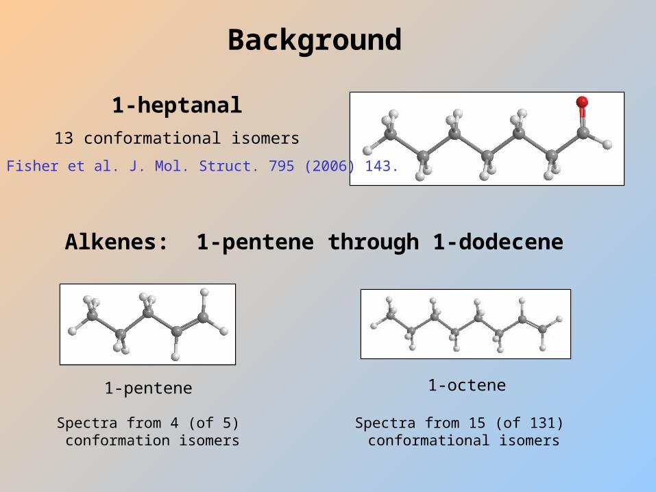
1-heptanal

13 conformational isomers

J. M. Fisher et al. J. Mol. Struct. 795 (2006) 143.

Alkenes: 1-pentene through 1-dodecene

Spectra from 4 (of 5) conformation isomers

Spectra from 15 (of 131) conformational isomers

1-pentene 1-octene

Background

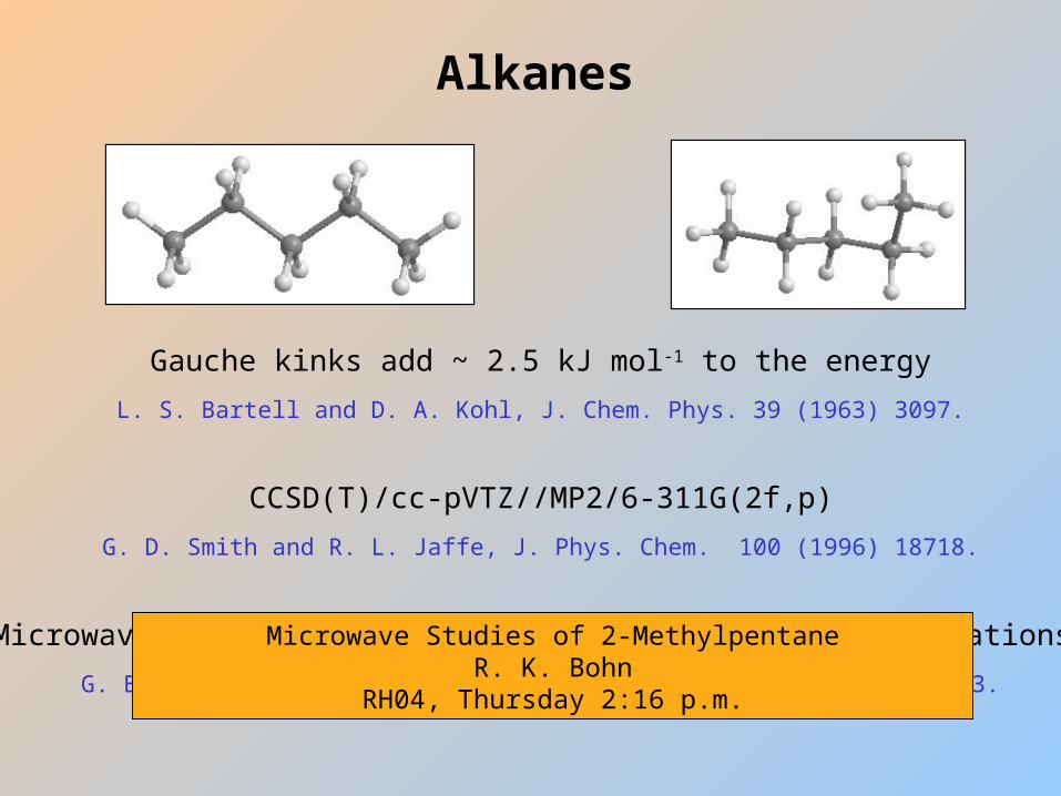
Gauche kinks add ~ 2.5 kJ mol-1 to the energy

L. S. Bartell and D. A. Kohl, J. Chem. Phys. 39 (1963) 3097.

G. D. Smith and R. L. Jaffe, J. Phys. Chem. 100 (1996) 18718.

CCSD(T)/cc-pVTZ//MP2/6-311G(2f,p)

Microwave spectra of anti-anti and anti-gauche configurations:

G. B. Churchill and R. K. Bohn, J. Phys. Chem. A 111 (2007) 3513.

Alkanes

Microwave Studies of 2-MethylpentaneR. K. Bohn

RH04, Thursday 2:16 p.m.

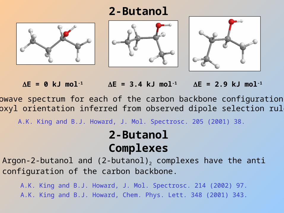
2-Butanol

Microwave spectrum for each of the carbon backbone configurations.Hydroxyl orientation inferred from observed dipole selection rules.

A.K. King and B.J. Howard, J. Mol. Spectrosc. 214 (2002) 97.

2-Butanol Complexes

Argon-2-butanol and (2-butanol)2 complexes have the anti configuration of the carbon backbone.

A.K. King and B.J. Howard, Chem. Phys. Lett. 348 (2001) 343.

A.K. King and B.J. Howard, J. Mol. Spectrosc. 205 (2001) 38.

E = 2.9 kJ mol-1E = 3.4 kJ mol-1E = 0 kJ mol-1

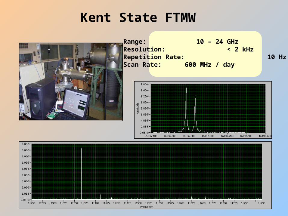
Kent State FTMW

Range: 10 – 24 GHzResolution: < 2 kHzRepetition Rate: 10 HzScan Rate: 600 MHz / day

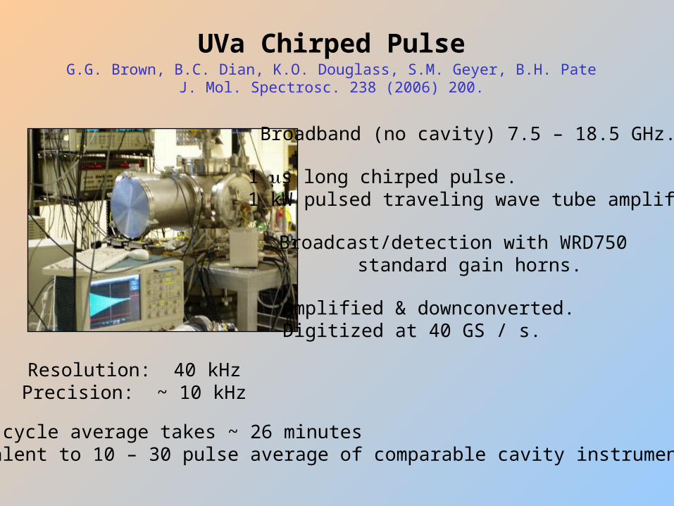
UVa Chirped PulseG.G. Brown, B.C. Dian, K.O. Douglass, S.M. Geyer, B.H. Pate

J. Mol. Spectrosc. 238 (2006) 200.

Broadband (no cavity) 7.5 – 18.5 GHz.

1 s long chirped pulse. 1 kW pulsed traveling wave tube amplifier.

Broadcast/detection with WRD750 standard gain horns.

Amplified & downconverted. Digitized at 40 GS / s.

Resolution: 40 kHzPrecision: ~ 10 kHz

10000 cycle average takes ~ 26 minutesEquivalent to 10 – 30 pulse average of comparable cavity instrument.

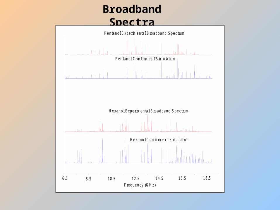
Broadband Spectra

6.5 8.5 10.5 12.5 14.5 16.5 18.5

Frequency (G H z)

H exanol Experim ental B roadband Spectrum

Pentanol Experim ental B roadband Spectrum

Pentanol C onform er I S im ulation

H exanol C onform er I S im ulation

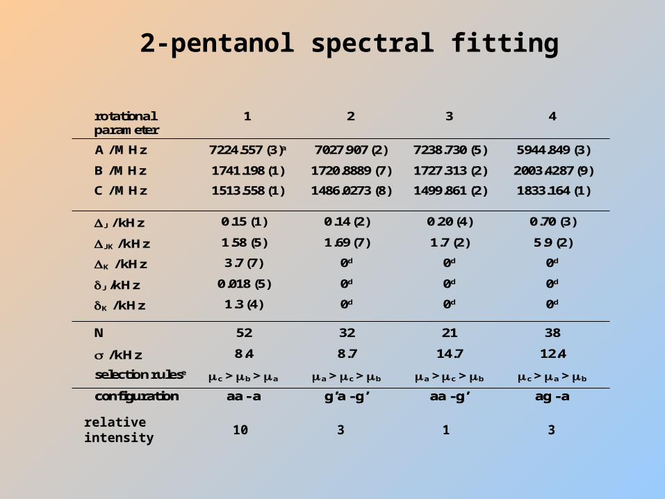
rotationalparameter

1 2 3 4

A / MHz 7224.557 (3)a 7027.907 (2) 7238.730 (5) 5944.849 (3)

B / MHz 1741.198 (1) 1720.8889 (7) 1727.313 (2) 2003.4287 (9)

C / MHz 1513.558 (1) 1486.0273 (8) 1499.861 (2) 1833.164 (1)

J / kHz 0.15 (1) 0.14 (2) 0.20 (4) 0.70 (3)

JK / kHz 1.58 (5) 1.69 (7) 1.7 (2) 5.9 (2)

K / kHz 3.7 (7) 0d 0d 0d

J /kHz 0.018 (5) 0d 0d 0d

K / kHz 1.3 (4) 0d 0d 0d

N 52 32 21 38

/ kHz 8.4 8.7 14.7 12.4

selection rulese c > b > a a > c > b a > c > b c > a > b

configuration aa - a g’a - g’ aa - g’ ag - aconfiguration aa - a g’a - g’ aa - g’ ag - a

2-pentanol spectral fitting

relativeintensity

10 33 1

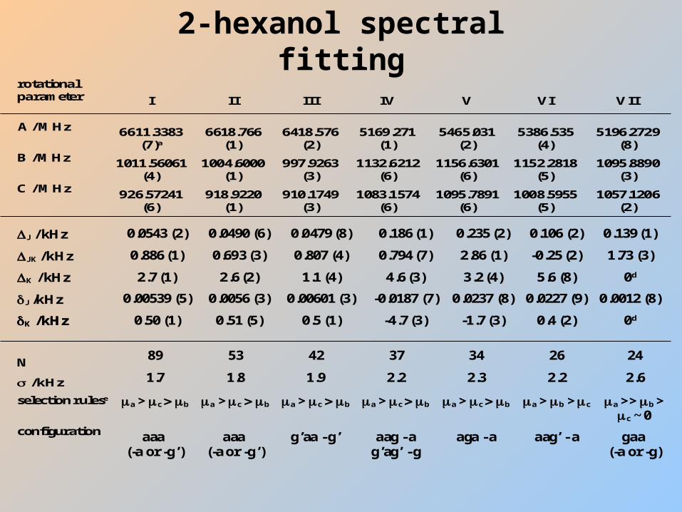
2-hexanol spectral fittingrotationalparameter

A / MHz

B / MHz

C / MHz

I II III IV V VI VII

6611.3383(7)a

6618.766(1)

6418.576(2)

5169.271(1)

5465.031(2)

5386.535(4)

5196.2729(8)

1011.56061(4)

1004.6000(1)

997.9263(3)

1132.6212(6)

1156.6301(6)

1152.2818(5)

1095.8890(3)

926.57241(6)

918.9220(1)

910.1749(3)

1083.1574(6)

1095.7891(6)

1008.5955(5)

1057.1206(2)

J / kHz

JK / kHz

K / kHz

J /kHz

K / kHzK / kHz

0.0543 (2) 0.0490 (6) 0.0479 (8) 0.186 (1) 0.235 (2) 0.106 (2) 0.139 (1)

0.886 (1) 0.693 (3) 0.807 (4) 0.794 (7) 2.86 (1) -0.25 (2) 1.73 (3)

2.7 (1) 2.6 (2) 1.1 (4) 4.6 (3) 3.2 (4) 5.6 (8) 0d

0.00539 (5) 0.0056 (3) 0.00601 (3) -0.0187 (7) 0.0237 (8) 0.0227 (9) 0.0012 (8)

0.50 (1) 0.51 (5) 0.5 (1) -4.7 (3) -1.7 (3) 0.4 (2) 0d

N

/ kHz

selection rulese

configuration

89 53 42 37 34 26 24

1.7 1.8 1.9 2.2 2.3 2.2 2.6

a > cb a > cb a > cb a > cb a > cb a > b > c a >> b >c ~ 0

aaa (-a or -g’)

aaa (-a or -g’)

g’aa - g’ aag - ag’ag’ - g

aga - a aag’ - a gaa (-a or -g)

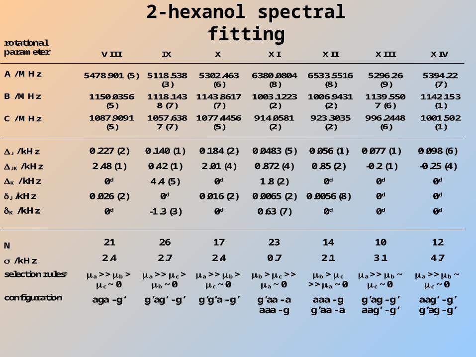
2-hexanol spectral fitting

VIII IX X XI XII XIII XIV

5478.901 (5) 5118.538(3)

5302.463(6)

6380.0804(8)

6533.5516(8)

5296.26(9)

5394.22(7)

1150.0356(5)

1118.1438 (7)

1143.8617(7)

1003.1223(2)

1006.9431(2)

1139.5507 (6)

1142.153(1)

1087.9091(5)

1057.6387 (7)

1077.4456(5)

914.0581(2)

923.3035(2)

996.2448(6)

1001.502(1)

0.227 (2) 0.140 (1) 0.184 (2) 0.0483 (5) 0.056 (1) 0.077 (1) 0.098 (6)

2.48 (1) 0.42 (1) 2.01 (4) 0.872 (4) 0.85 (2) -0.2 (1) -0.25 (4)

0d 4.4 (5) 0d 1.8 (2) 0d 0d 0d

0.026 (2) 0d 0.016 (2) 0.0065 (2) 0.0056 (8) 0d 0d

0d -1.3 (3) 0d 0.63 (7) 0d 0d 0d

rotationalparameter

A / MHz

B / MHz

C / MHz

J / kHz

JK / kHz

K / kHz

J /kHz

K / kHzK / kHz

N

/ kHz

selection rulese

configuration

21 26 17 23 14 10 12

2.4 2.7 2.4 0.7 2.1 3.1 4.7

a >> b >c ~ 0

a >> c >b ~ 0

a >> b >c ~ 0

b > c >>a ~ 0

b > c

>> a ~ 0a >> b ~

c ~ 0a >> b ~

c ~ 0

aga - g’ g’ag’ - g’ g’g’a - g’ g’aa - aaaa - g

aaa - gg’aa - a

g’ag - g’aag’ - g’

aag’ - g’g’ag - g’

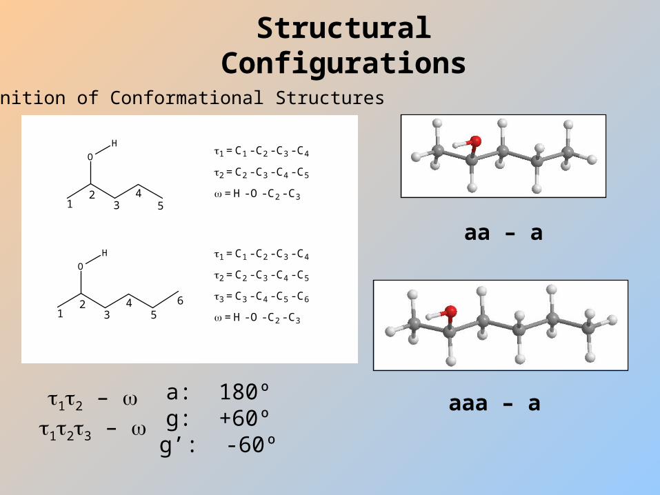
Structural Configurations

Definition of Conformational Structures

O

12

34 6

H

O

12

34

5

H

5

1 = C1 - C2 - C3 - C4

3 = C3 - C4 - C5 - C6

= H - O - C2 - C3

1 = C1 - C2 - C3 - C4

2 = C2 - C3 - C4 - C5

2 = C2 - C3 - C4 - C5

= H - O - C2 - C3

a: 180ºg: +60ºg’: -60º

12 – 123 –

aaa – a

aa – a

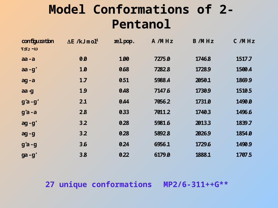
Model Conformations of 2-Pentanol

configuration1122 -

E / kJ mol-1-1 rel. pop. A / MHz B / MHz C / MHz

aa - a 0.0 1.00 7275.0 1746.8 1517.7

aa - g’ 1.0 0.68 7282.8 1728.9 1500.4

ag - a 1.7 0.51 5988.4 2050.1 1869.9

aa -g 1.9 0.48 7147.6 1730.9 1510.5

g’a - g’ 2.1 0.44 7056.2 1731.0 1490.0

g’a - a 2.8 0.33 7011.2 1740.3 1496.6

ag - g’ 3.2 0.28 5981.6 2013.3 1839.7

ag - g 3.2 0.28 5892.8 2026.9 1854.0

g’a - g 3.6 0.24 6956.1 1729.6 1490.9

ga - g’ 3.8 0.22 6179.0 1888.1 1707.5

MP2/6-311++G**27 unique conformations

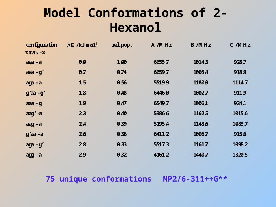
Model Conformations of 2-Hexanol

MP2/6-311++G**75 unique conformations

configuration112233 -

E / kJ mol-1-1 rel. pop. A / MHz B / MHz C / MHz

aaa - a 0.0 1.00 6655.7 1014.3 928.7

aaa - g’ 0.7 0.74 6659.7 1005.4 918.9

aga - a 1.5 0.56 5519.9 1180.0 1114.7

g’aa - g’ 1.8 0.48 6446.0 1002.7 911.9

aaa - g 1.9 0.47 6549.7 1006.1 924.1

aag’ -a 2.3 0.40 5386.6 1162.5 1015.6

aag - a 2.4 0.39 5195.4 1143.6 1083.7

g’aa - a 2.6 0.36 6411.2 1006.7 915.6

aga - g’ 2.8 0.33 5517.3 1161.7 1098.2

agg - a 2.9 0.32 4161.2 1440.7 1320.5

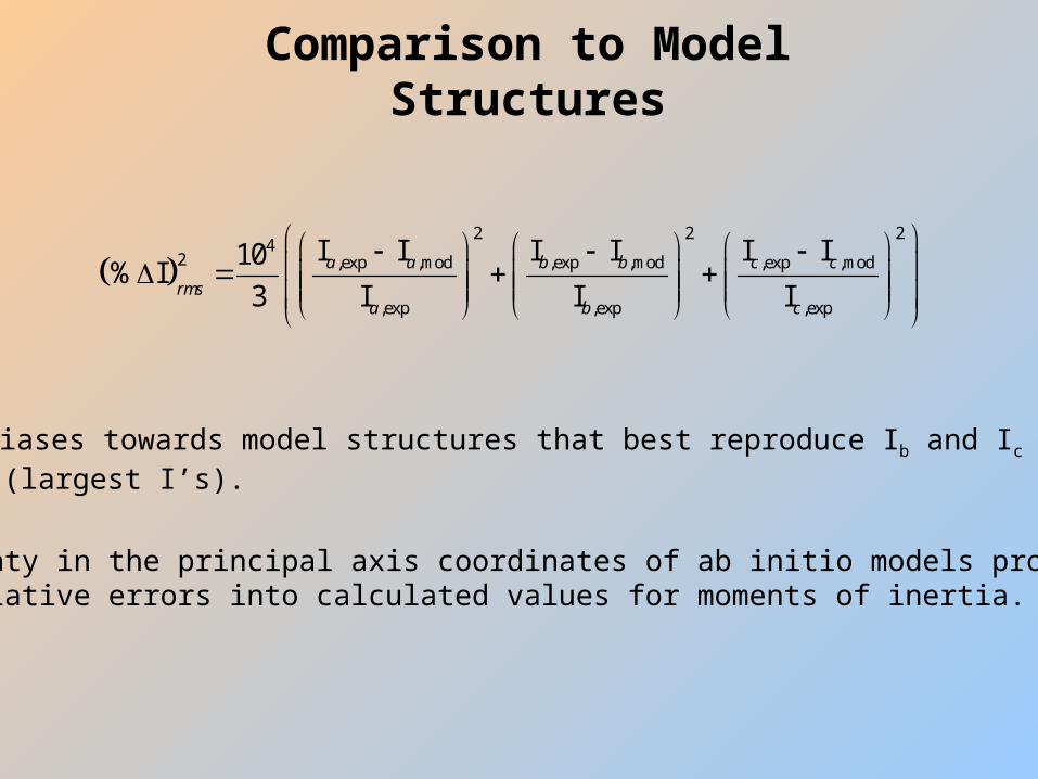
Comparison to Model Structures

2 2 2

42 ,exp ,mod ,exp ,mod ,exp ,mod

,exp ,exp ,exp

I I I I I I10% I

3 I I Ia a b b c c

rmsa b c

Irms biases towards model structures that best reproduce Ib and Ic (largest I’s).

Uncertainty in the principal axis coordinates of ab initio models propagates as relative errors into calculated values for moments of inertia.

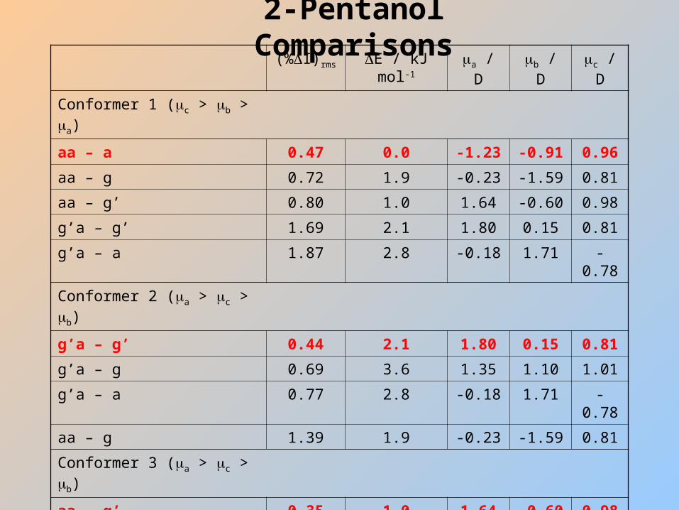
2-Pentanol Comparisons(%I)rms E / kJ mol-1 a / D b / D c / D

Conformer 1 (c > b > a)

aa – a 0.47 0.0 -1.23 -0.91 0.96

aa – g 0.72 1.9 -0.23 -1.59 0.81

aa – g’ 0.80 1.0 1.64 -0.60 0.98

g’a – g’ 1.69 2.1 1.80 0.15 0.81

g’a – a 1.87 2.8 -0.18 1.71 -0.78

Conformer 2 (a > c > b)

g’a – g’ 0.44 2.1 1.80 0.15 0.81

g’a – g 0.69 3.6 1.35 1.10 1.01

g’a – a 0.77 2.8 -0.18 1.71 -0.78

aa – g 1.39 1.9 -0.23 -1.59 0.81

Conformer 3 (a > c > b)

aa – g’ 0.35 1.0 1.64 -0.60 0.98

aa – g 0.85 1.9 -0.23 -1.59 0.81

aa – a 0.98 0.0 -1.23 -0.91 0.96

g’a – g’ 1.55 2.1 1.80 0.15 0.81

g’a – a 1.93 2.8 -0.18 1.71 -0.78

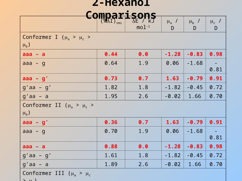
2-Hexanol Comparisons(%I)rms E / kJ mol-1 a / D b / D c / D

Conformer I (a > c > b)

aaa – a 0.44 0.0 -1.28 -0.83 0.98

aaa – g 0.64 1.9 0.06 -1.68 -0.81

aaa – g’ 0.73 0.7 1.63 -0.79 0.91

g’aa – g’ 1.82 1.8 -1.82 -0.45 0.72

g’aa – a 1.95 2.6 -0.02 1.66 0.70

Conformer II (a > c > b)

aaa – g’ 0.36 0.7 1.63 -0.79 0.91

aaa – g 0.70 1.9 0.06 -1.68 -0.81

aaa – a 0.88 0.0 -1.28 -0.83 0.98

g’aa – g’ 1.61 1.8 -1.82 -0.45 0.72

g’aa – a 1.89 2.6 -0.02 1.66 0.70

Conformer III (a > c > b)

g’aa – g’ 0.38 1.8 -1.82 -0.45 0.72

g’aa – g 0.52 3.3 1.44 0.87 1.12

g’aa – a 0.61 2.6 -0.02 1.66 0.70

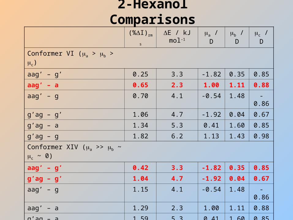
2-Hexanol Comparisons

(%I)rms E / kJ mol-1 a / D b / D c / D

Conformer VI (a > b > c)

aag’ – g’ 0.25 3.3 -1.82 0.35 0.85

aag’ – a 0.65 2.3 1.00 1.11 0.88

aag’ – g 0.70 4.1 -0.54 1.48 -0.86

g’ag – g’ 1.06 4.7 -1.92 0.04 0.67

g’ag – a 1.34 5.3 0.41 1.60 0.85

g’ag – g 1.82 6.2 1.13 1.43 0.98

Conformer XIV (a >> b ~ c ~ 0)

aag’ – g’ 0.42 3.3 -1.82 0.35 0.85

g’ag – g’ 1.04 4.7 -1.92 0.04 0.67

aag’ – g 1.15 4.1 -0.54 1.48 -0.86

aag’ – a 1.29 2.3 1.00 1.11 0.88

g’ag – a 1.59 5.3 0.41 1.60 0.85

g’ag – g 1.89 6.2 1.13 1.43 0.98

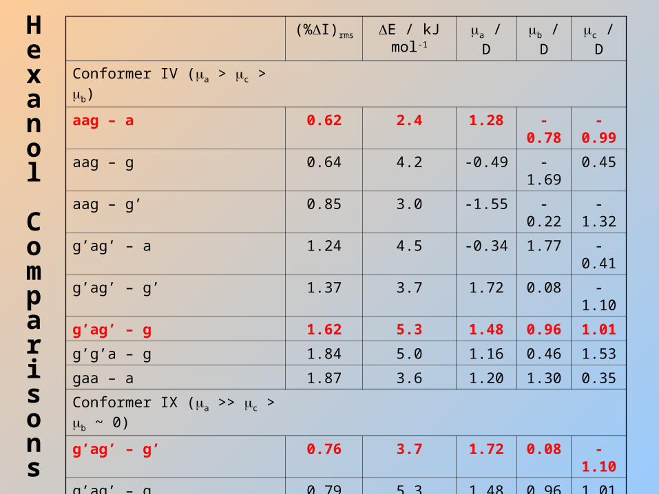
(%I)rms E / kJ mol-1 a / D b / D c / D

Conformer IV (a > c > b)

aag – a 0.62 2.4 1.28 -0.78 -0.99

aag – g 0.64 4.2 -0.49 -1.69 0.45

aag – g’ 0.85 3.0 -1.55 -0.22 -1.32

g’ag’ – a 1.24 4.5 -0.34 1.77 -0.41

g’ag’ – g’ 1.37 3.7 1.72 0.08 -1.10

g’ag’ – g 1.62 5.3 1.48 0.96 1.01

g’g’a – g 1.84 5.0 1.16 0.46 1.53

gaa – a 1.87 3.6 1.20 1.30 0.35

Conformer IX (a >> c > b ~ 0)

g’ag’ – g’ 0.76 3.7 1.72 0.08 -1.10

g’ag’ – g 0.79 5.3 1.48 0.96 1.01

g’ag’ – a 1.16 4.5 -0.34 1.77 -0.41

gaa – a 1.19 3.6 1.20 1.30 0.35

gaa – g’ 1.30 3.5 -0.62 -0.19 1.69

aag – g’ 1.41 3.0 -1.55 -0.22 -1.32

aag – g 1.59 4.2 -0.49 -1.69 0.45

gaa – g 1.88 5.7 -1.34 1.53 -0.03

Hexanol Comparisons

Conformational Assignment

1aa – a

2g’a – g’

3aa – g’

4ag – a

Iaaa – aaaa – g’

IIaaa – g’aaa – a

IIIg’aa – g’g’aa – g

IVaag – a

g’ag’ – g

Vaga – a

VIaag’ – a

VIIgaa – agaa – g

VIIIaga – g’

IXg’ag’ – g’

Xg’g’a – g’

XIg’aa – aaaa – g

XIIaaa – gg’aa – a

XIIIg’ag – g’aag’ – g’

XIVaag’ – g’g’ag – g’

2-Hexanol

2-Pentanol

Acknowledgments

National Science Foundation (CHE-0240168 and CHE-0616660)

Ohio Supercomputer Center

National Science Foundation Major Resource Instrumentation Program (0215957)