Embed Size (px)
Citation preview
The Americas Flow Measurement Conference
1-2 May 2013
Technical Paper
1
GAS CHROMATOGRAPHY MAINTENANCE USING
UNCERTAINTY BASED CBM
Anwar Sutan, i-Vigilant Technologies
Paul Daniel, i-Vigilant Technologies
1 INTRODUCTION
On-line gas chromatography is frequently used within Fiscal and Custody Transfer measurement systems. The uncertainty of the analysis from the gas chromatograph (GC) is of the utmost importance with the resultant analysis frequently at the core of economic transactions.
The modern gas chromatograph is an extremely repeatable device, however to ensure that the system remains both accurate and repeatable requires that suitable monitoring and maintenance are in place.
Even though a GC may be repeatable it does not preclude the possibility of systematic errors. A systematic error may ensue due to several different reasons. These may include such things as poor calibration gas handling resulting in a non-homogenous reference mixture, unsuitable selection of the reference gas mixture resulting in biases due to linearity or the assumed response functions, peak drifts, valve leakage etc. A recent study performed by the author identified a situation where a systematic error was observed, which if remained undetected, would have resulted in an on-going error in the calorific value of up to 1.4%. This error equated to a value of more than $200,000 per month.
Once reasonable steps have been taken to ensure that the system is free from systematic error then, under the assumption of suitable sampling and conditioning, the uncertainty of the GC measurement is generally driven by the repeatability of the GC and the quality of the (certified) reference gas mixture. There are various methods which may be used to obtain the GC repeatability. ISO 10723 describes a method of performance evaluation using multiple calibration gas compositions to obtain the linearity of the GC as well as its repeatability. ASTM D1945 provides a standard test method for the analysis of gas with a GC with stated levels for the expected repeatability and reproducibility. However, these methods are only valid as long as the GC maintains the performance characteristics measured on the day of the test. To ensure the GC remains repeatable over a prolonged period of operation on-going monitoring is required.
This paper presents a novel philosophy for determining both the initial health of the GC and for the continued monitoring and assessment of the GC performance. The result is an ability to provide an on-line estimate of the repeatability of each component allowing the overall uncertainty in the Calorific Value to be established (or any other parameter calculated from composition). The philosophy will be demonstrated using real data from several case studies to illustrate how an
‘expert system’ may be used to provide the uncertainty of the GC as well as an indication of when the GC needs to be serviced, thereby providing assurance that the GC is operating within specified limits and meeting contractual obligations.
The Americas Flow Measurement Conference
1-2 May 2013
Technical Paper
2
2 Gas Chromatograph Design and Operation
A multi-column separation technique is required to get the composition of a natural gas with inert components and hydrocarbon components ranging from C1 to C7+ in a practical time frame and without temperature ramping.
The three column GC design is consistent with ISO 6974-5:2000 [3]. It uses three columns, a restrictor and two detectors housed in a controlled temperature
chamber. The detectors are usually thermal conductivity detectors (thermistors), where the resistance is a function of the temperature. The reference and measurement detectors form a balanced Wheatstone-Bridge. Helium is the preferred carrier gas because it has a relatively high thermal conductivity. With only carrier gas flowing across the two detectors, the Wheatstone bridge is in balance. As the sample gases pass across the measuring detector the change in gas thermal conductivity results in a change in the rate of heat exchange between
the thermistor and the surrounding gas which results in a change in the thermistor temperature. The change of temperature causes a change of resistance in the measurement detector, thus unbalancing the Wheatstone-Bridge. The magnitude of the voltage created by the unbalanced bridge and the time taken for the gas to pass across the detector forms a response curve proportional to the amount of the component in the carrier gas stream. The area under the response curve is proportional to the mol percentage of component
being measured. The actual value of the component is determined by comparison of the measured response to the response obtained from a gas of known composition, usually referred to as the calibration gas.
On a single column GC where pressure, temperature, and flow rate is maintained at a constant rate, there is a very high correlation between the molecular weight of the saturated gas components and their response factors. With a three-column
GC, restrictor tubing has to be applied to regulate the carrier gas flow to maintain and achieve a close-to-constant flow rate during valve actuation operations. Even with the pressure and temperature maintained constant, and with a restrictor tubing in place, slight flow rate differences still occur, thereby changing the response of the thermal conductivity detector. These fluctuations in flow rate reduce the correlation between the molecular weight of each component and its corresponding response factor.
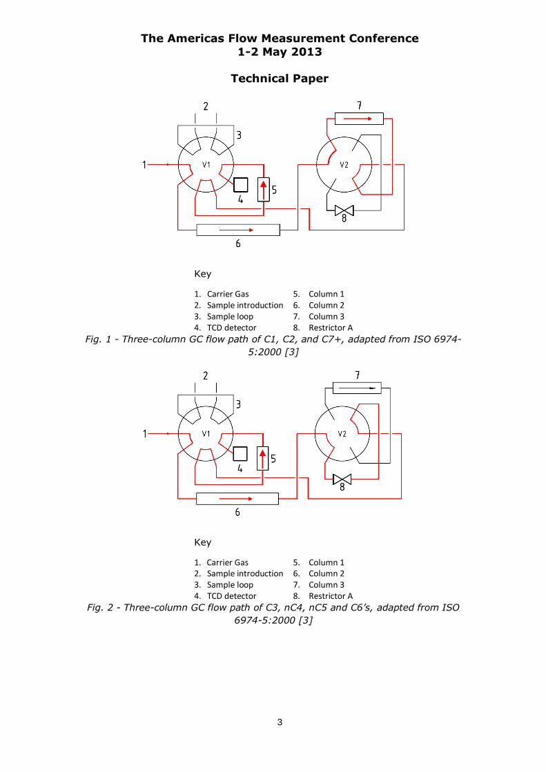
For a three column GC, Fig. 1 shows the GC flow tubing path configuration for C1, N2, CO2, C2 and C7+. Similarly Fig. 2 shows the flow tubing path of C3, iC4, nC4, neoC5, nC5, C6’s. Any difference in the effective restriction presented by the restrictor tubing and column 3 would result in a difference in the flow rate between the two path configurations.
The Americas Flow Measurement Conference
1-2 May 2013
Technical Paper
3
Key
1. Carrier Gas 2. Sample introduction 3. Sample loop 4. TCD detector
5. Column 1 6. Column 2 7. Column 3 8. Restrictor A
Fig. 1 - Three-column GC flow path of C1, C2, and C7+, adapted from ISO 6974-
5:2000 [3]
Key
1. Carrier Gas 2. Sample introduction 3. Sample loop 4. TCD detector
5. Column 1 6. Column 2 7. Column 3 8. Restrictor A
Fig. 2 - Three-column GC flow path of C3, nC4, nC5 and C6’s, adapted from ISO
6974-5:2000 [3]
The Americas Flow Measurement Conference
1-2 May 2013
Technical Paper
4
3 The Underlying Issues
Gas Chromatographs are, generally speaking, highly repeatable devices. In a number of situations, such a description can give a false sense of security, since repeatability may sometimes be incorrectly interpreted as accuracy. This is not the case. If configured incorrectly, the GC would give consistently and repeatedly the wrong result. This can happen for various reasons among which might be the incorrect handling of the calibration gas, poor quality of calibration gas, or valve
timing issues.
The systematic drift of the response factors can be indicative of a number of problems. However, the detection of this through automatic GC calibration is not always possible. This is because the usual method of detection is to compare the shift between successive automatic calibrations. However, a gradual change in the response factor can easily result in a shift that remains within the tolerance
limit set in the GC controller and hence continue without detection. Even with the incorrect calibration result, the GC can continue to give repeatable results. However, the results will not be accurate and the uncertainty of the measurement will invariably be increased.
The common industry practice in the UK is to have the GC audited / maintained by a specialist once a year. The GC is then expected to continue to perform within
the uncertainty limit observed during the maintenance procedure. However, the GC performance and its uncertainty limit will only be valid if the GC continues to maintain the same performance characteristics as measured and recorded on the day of the calibration. If there is any shift in the characteristics of the GC, or the operating conditions, then the uncertainty statement made on the day of the annual maintenance will no longer be valid.
The uncertainty of the CV from a healthy GC is normally within the range of ±0.1 MJ/m3. The results from one of the case studies performed has identified a scenario where an error of up to 1.4% or 0.63 MJ/m3 was present in the calculated CV due to incorrect calibration. This figure is 6 times greater than the nominal uncertainty level of the device and would have been very likely to remain undetected without the use of condition based monitoring tool.
Current Practice 3.1
Within the UK North Sea the following steps are generally taken to ensure that the performance of the GC is maintained at a satisfactory level:
1. Periodic health check by a GC specialist.
2. ISO 10723 multilevel calibration to determine the GC linearity and measurement bias.
3. Regular calibration using a certified working reference mixture.
4. Periodic repeatability check using the tolerances provided by ASTM 1945D.
It is common for all these activities to be performed by different parties. The result is a number of different reports that need to be combined and reviewed as a whole to obtain the full picture of the GC performance.
The following sections provide very brief overview of the available methods and standards presently in common use.
The Americas Flow Measurement Conference
1-2 May 2013
Technical Paper
5
3.1.1 ISO 10723
ISO 10723 [2] is a standard relating to the performance evaluation for online analytical systems. It has gained particular prevalence in Europe following the publication of the EUETS measurement and reporting guidelines [4] where annually repeated validation by an EN ISO 17025:2005 [6] accredited laboratory was specified.
A number of test gases are used to establish:
The ability of the GC to measure the components specified.
The repeatability of the measurement of each component over their specified ranges.
The relationship between response and concentration of each component over their specified ranges.
3.1.2 ASTM D 1945
This defines a standard test method for the analysis of natural gas by gas chromatography. Of particular interest to this paper are the sections that detail repeatability and reproducibility.
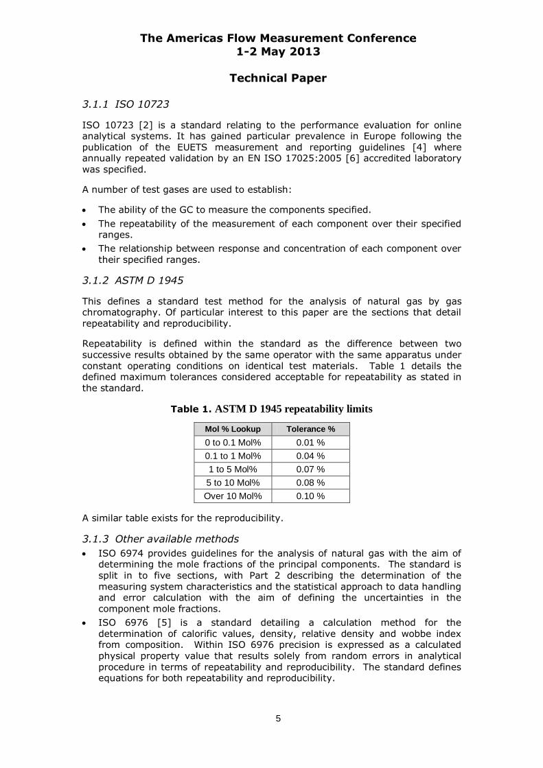
Repeatability is defined within the standard as the difference between two successive results obtained by the same operator with the same apparatus under constant operating conditions on identical test materials. Table 1 details the defined maximum tolerances considered acceptable for repeatability as stated in the standard.
Table 1. ASTM D 1945 repeatability limits
Mol % Lookup Tolerance %
0 to 0.1 Mol% 0.01 %
0.1 to 1 Mol% 0.04 %
1 to 5 Mol% 0.07 %
5 to 10 Mol% 0.08 %
Over 10 Mol% 0.10 %
A similar table exists for the reproducibility.
3.1.3 Other available methods
ISO 6974 provides guidelines for the analysis of natural gas with the aim of determining the mole fractions of the principal components. The standard is
split in to five sections, with Part 2 describing the determination of the measuring system characteristics and the statistical approach to data handling and error calculation with the aim of defining the uncertainties in the component mole fractions.
ISO 6976 [5] is a standard detailing a calculation method for the determination of calorific values, density, relative density and wobbe index from composition. Within ISO 6976 precision is expressed as a calculated
physical property value that results solely from random errors in analytical procedure in terms of repeatability and reproducibility. The standard defines equations for both repeatability and reproducibility.
The Americas Flow Measurement Conference
1-2 May 2013
Technical Paper
6
Application of some fundamental methodologies and utilization of Gas
Chromatography Analysis Software (GCAS®) can assist not only in identifying the for mentioned problems, but also in formulating an implementation plan to rectify or eliminate them. Collection of the required calibration data and utilization of all of the tools from GCAS® will allow the industry to achieve the advantages and be able to:
Maintain GC accuracy throughout the year
Eliminate unnecessary error
Predict future failure
Help support and increase technician’s competency level
Reduce unnecessary specialist cost
Provide guidelines as to the necessary course of action to rectify failures
Create a fully auditable database of GC performance
4 THE PROPOSED METHOD
The common practice of performing distinct tests by different vendors at different times has led to the realisation that there are distinct advantages associated with collating all the information from the GC maintenance activities in to one place, combining all the data and results and presenting it in a clear, concise and easily interpreted manner. This information, when used in conjunction with a number of additional novel techniques, results in a condition based monitoring system with an expert system capability providing early detection of potential GC failures coupled with the ability to assist with the determination of the required course of actions to rectify any identified problems.
The proposed method consists of the following:
1. Acquisition of GC analysis parameters.
2. Analysis of events timing.
3. Analysis of individual calibration data prior to use as a foot-print.
4. Analysis of each calibration and comparison with the foot-print data.
5. Analysis of historical data.
6. Acquisition of working reference mixture uncertainty.
7. Analysis of repeatability.
8. Extended reproducibility assessment providing the basis for a live uncertainty calculation.
9. Estimation of the bias based on the ISO 10723 performance evaluation method.
The result of this is an expert system which can provide a live estimate of the uncertainty incorporating the uncertainty of the working reference mixture used for routine calibration, the repeatability and the long term reproducibility. An estimate of the uncertainty of other calculated parameters such as density and calorific value may also be determined.
Knowledge of the live operating uncertainty not only provides assurance that the measurement is meeting the required specification, but may also be used to determine when maintenance of the GC needs to be performed.
The Americas Flow Measurement Conference
1-2 May 2013
Technical Paper
7
Steps one to five are covered by section 4.1. The remaining items are discussed
with a working example using live data from an operational GC.
Foot-printing and analysis of historical data 4.1
A previous publication in 2009 described a method to analyse three-column gas chromatographs using the correlation between the component’s molecular weights and their response factors [9].
This method lead to a condition based monitoring philosophy, GCAS®, which utilises the techniques described within the paper to ensure that the status of a GC is healthy prior to foot-printing.
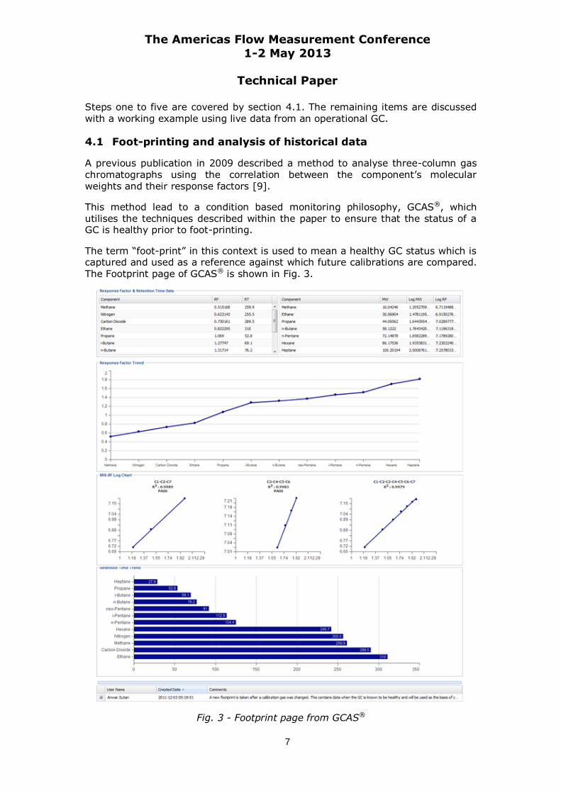
The term “foot-print” in this context is used to mean a healthy GC status which is captured and used as a reference against which future calibrations are compared.
The Footprint page of GCAS® is shown in Fig. 3.
Fig. 3 - Footprint page from GCAS®
The Americas Flow Measurement Conference
1-2 May 2013
Technical Paper
8
4.1.1 Response Factor (RF) and Retention Time (RT) Data
The Response Factor and Retention Time Data show the raw data of the response factor (RF) and retention time for each of the components, as well as the logarithm of the Molecular Weight (MW) and RF. This data is processed and presented through graphical trends for analysis. The Response factor and retention time data in the footprint page are shown in the first part of Fig. 3.
4.1.2 Response Factor Trend
The relationship between thermal conductivity and Molecular weight in hydrocarbon and inert gases is well known. The larger the molecular weight the lower the thermal conductivity.
The temperature of the thermistor changes whenever gas with a different thermal conductivity flows across it. The change in the temperature is dependent on the amount of the component (mole %) and the response of the thermistor to each component (Response Factor). The greater the difference in the thermal conductivity between the carrier gas and the component being measured, the greater the temperature change. Hence a gas with a much lower thermal conductivity than the carrier gas will result in larger response factor.
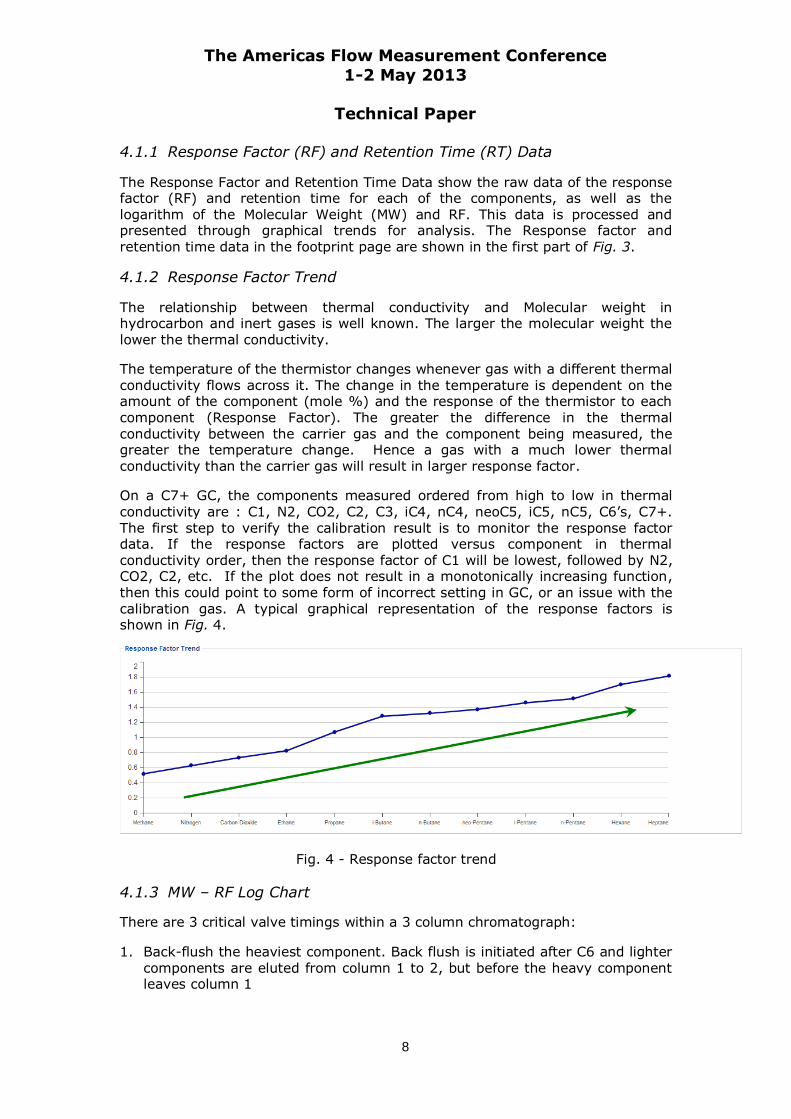
On a C7+ GC, the components measured ordered from high to low in thermal
conductivity are : C1, N2, CO2, C2, C3, iC4, nC4, neoC5, iC5, nC5, C6’s, C7+. The first step to verify the calibration result is to monitor the response factor data. If the response factors are plotted versus component in thermal conductivity order, then the response factor of C1 will be lowest, followed by N2, CO2, C2, etc. If the plot does not result in a monotonically increasing function, then this could point to some form of incorrect setting in GC, or an issue with the calibration gas. A typical graphical representation of the response factors is shown in Fig. 4.
Fig. 4 - Response factor trend
4.1.3 MW – RF Log Chart
There are 3 critical valve timings within a 3 column chromatograph:
1. Back-flush the heaviest component. Back flush is initiated after C6 and lighter components are eluted from column 1 to 2, but before the heavy component leaves column 1
The Americas Flow Measurement Conference
1-2 May 2013
Technical Paper
9
2. Trap the light components in column 3. The valve actuation has to be done
after all C2 is eluted into column 3, but before any C3 leaves column 2
3. Allow lights to leave column 3. Valve actuation has to be done after all the middle components clear the measurement detector
Valve-timing errors can result in the emergence of following situations:
Some of the heavy components leave column 1 and flow through column 2
Some of the middle components are back-flushed together with the heavy components
Some C2 is left in column 2 after the valve 3 actuation to trap the lights
Some C3 goes in to column 3 before valve 3 actuation to trap the lights
Splitting of the first and last components on the column resulting in extraneous peaks on the chromatogram
Extraneous peaks within the peak window of calibrated peaks may be recognized as the calibrated peaks
The impact of these valve timing issues will influence the correlation of the components. Any valve timing issues will reduce the correlation between components. The correlation between MW and RF is shown in Fig. 5.
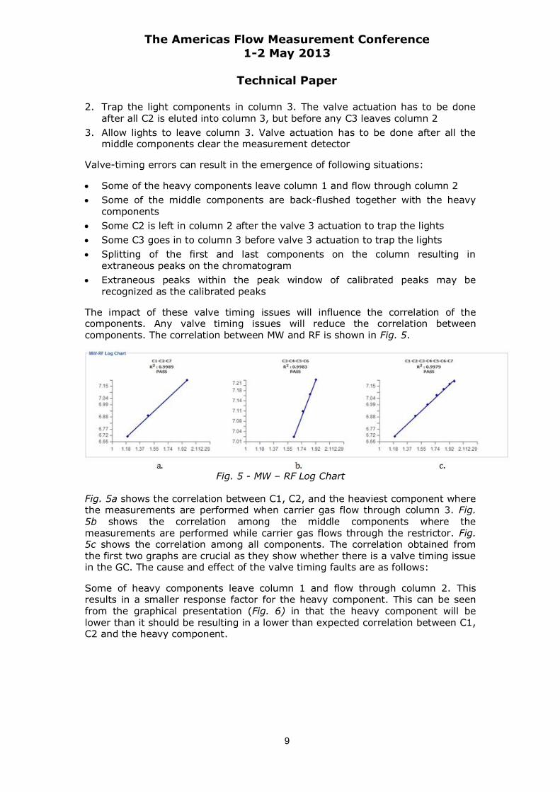
Fig. 5 - MW – RF Log Chart
Fig. 5a shows the correlation between C1, C2, and the heaviest component where the measurements are performed when carrier gas flow through column 3. Fig.
5b shows the correlation among the middle components where the measurements are performed while carrier gas flows through the restrictor. Fig. 5c shows the correlation among all components. The correlation obtained from the first two graphs are crucial as they show whether there is a valve timing issue in the GC. The cause and effect of the valve timing faults are as follows:
Some of heavy components leave column 1 and flow through column 2. This results in a smaller response factor for the heavy component. This can be seen from the graphical presentation (Fig. 6) in that the heavy component will be lower than it should be resulting in a lower than expected correlation between C1, C2 and the heavy component.
The Americas Flow Measurement Conference
1-2 May 2013
Technical Paper
10
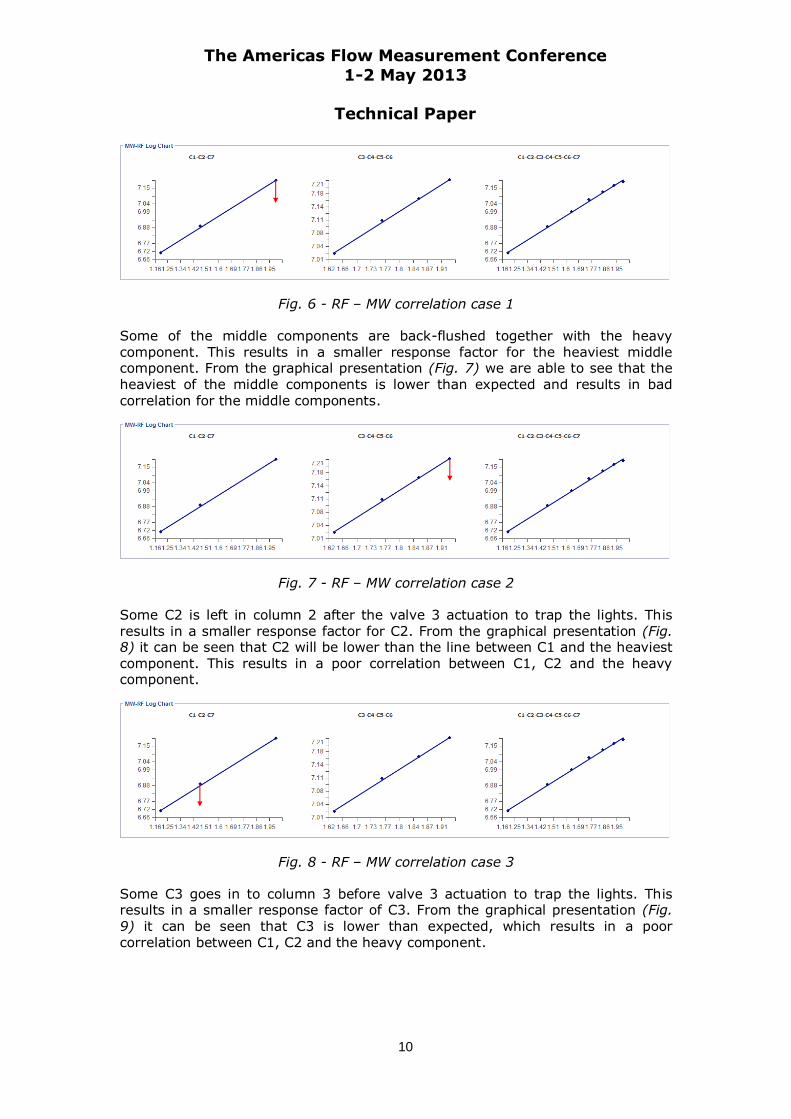
Fig. 6 - RF – MW correlation case 1
Some of the middle components are back-flushed together with the heavy component. This results in a smaller response factor for the heaviest middle component. From the graphical presentation (Fig. 7) we are able to see that the heaviest of the middle components is lower than expected and results in bad
correlation for the middle components.
Fig. 7 - RF – MW correlation case 2
Some C2 is left in column 2 after the valve 3 actuation to trap the lights. This results in a smaller response factor for C2. From the graphical presentation (Fig. 8) it can be seen that C2 will be lower than the line between C1 and the heaviest component. This results in a poor correlation between C1, C2 and the heavy component.
Fig. 8 - RF – MW correlation case 3
Some C3 goes in to column 3 before valve 3 actuation to trap the lights. This results in a smaller response factor of C3. From the graphical presentation (Fig. 9) it can be seen that C3 is lower than expected, which results in a poor correlation between C1, C2 and the heavy component.
The Americas Flow Measurement Conference
1-2 May 2013
Technical Paper
11
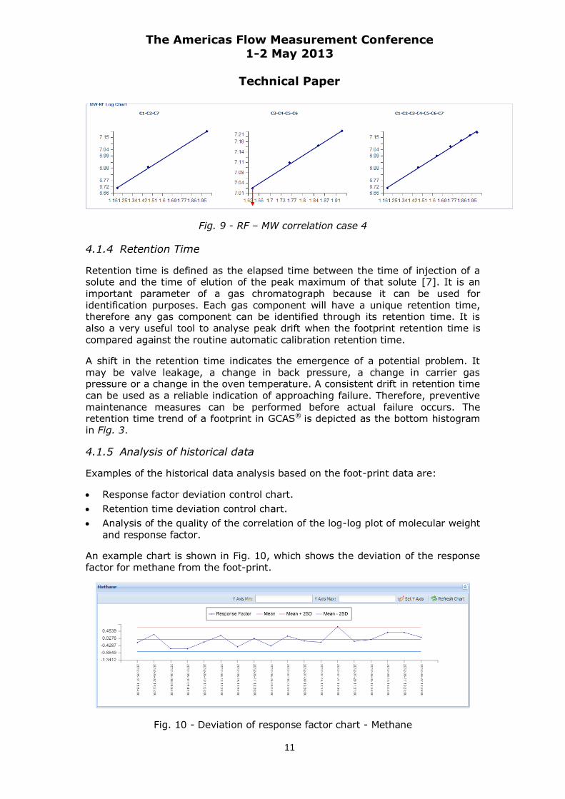
Fig. 9 - RF – MW correlation case 4
4.1.4 Retention Time
Retention time is defined as the elapsed time between the time of injection of a solute and the time of elution of the peak maximum of that solute [7]. It is an important parameter of a gas chromatograph because it can be used for identification purposes. Each gas component will have a unique retention time, therefore any gas component can be identified through its retention time. It is also a very useful tool to analyse peak drift when the footprint retention time is compared against the routine automatic calibration retention time.
A shift in the retention time indicates the emergence of a potential problem. It may be valve leakage, a change in back pressure, a change in carrier gas pressure or a change in the oven temperature. A consistent drift in retention time can be used as a reliable indication of approaching failure. Therefore, preventive maintenance measures can be performed before actual failure occurs. The retention time trend of a footprint in GCAS® is depicted as the bottom histogram in Fig. 3.
4.1.5 Analysis of historical data
Examples of the historical data analysis based on the foot-print data are:
Response factor deviation control chart.
Retention time deviation control chart.
Analysis of the quality of the correlation of the log-log plot of molecular weight and response factor.
An example chart is shown in Fig. 10, which shows the deviation of the response factor for methane from the foot-print.
Fig. 10 - Deviation of response factor chart - Methane
The Americas Flow Measurement Conference
1-2 May 2013
Technical Paper
12
Case Studies 4.2
Several case studies have been performed on different types of GC (C6+ and C7+). All the case studies have been performed remotely with the help of offshore metering technicians.
4.2.1 Calibration issue
The first case study was performed on a C6+ GC. The GC had been offline for some time and was to be brought back in to service. In order to bring the GC online, it was fitted with new calibration gas and a forced calibration was performed. By doing this, the GC accepted all calibration parameters (i.e. RF and RT). However, inspection of the Response Factor plot, Fig. 11, clearly indicated that the GC was not healthy.
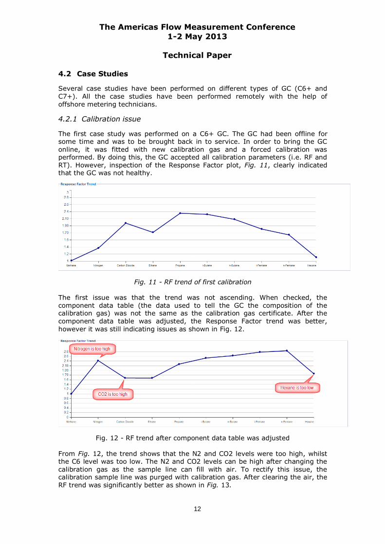
Fig. 11 - RF trend of first calibration
The first issue was that the trend was not ascending. When checked, the component data table (the data used to tell the GC the composition of the calibration gas) was not the same as the calibration gas certificate. After the component data table was adjusted, the Response Factor trend was better, however it was still indicating issues as shown in Fig. 12.
Fig. 12 - RF trend after component data table was adjusted
From Fig. 12, the trend shows that the N2 and CO2 levels were too high, whilst the C6 level was too low. The N2 and CO2 levels can be high after changing the calibration gas as the sample line can fill with air. To rectify this issue, the calibration sample line was purged with calibration gas. After clearing the air, the RF trend was significantly better as shown in Fig. 13.
The Americas Flow Measurement Conference
1-2 May 2013
Technical Paper
13
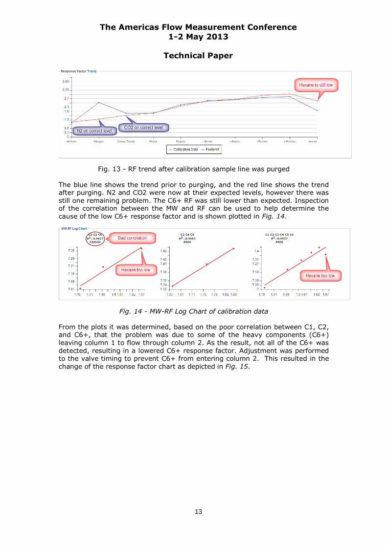
Fig. 13 - RF trend after calibration sample line was purged
The blue line shows the trend prior to purging, and the red line shows the trend after purging. N2 and CO2 were now at their expected levels, however there was still one remaining problem. The C6+ RF was still lower than expected. Inspection of the correlation between the MW and RF can be used to help determine the cause of the low C6+ response factor and is shown plotted in Fig. 14.
Fig. 14 - MW-RF Log Chart of calibration data
From the plots it was determined, based on the poor correlation between C1, C2, and C6+, that the problem was due to some of the heavy components (C6+) leaving column 1 to flow through column 2. As the result, not all of the C6+ was detected, resulting in a lowered C6+ response factor. Adjustment was performed to the valve timing to prevent C6+ from entering column 2. This resulted in the change of the response factor chart as depicted in Fig. 15.
The Americas Flow Measurement Conference
1-2 May 2013
Technical Paper
14
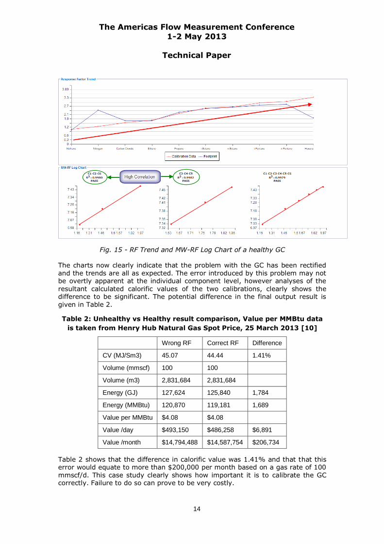
Fig. 15 - RF Trend and MW-RF Log Chart of a healthy GC
The charts now clearly indicate that the problem with the GC has been rectified and the trends are all as expected. The error introduced by this problem may not be overtly apparent at the individual component level, however analyses of the resultant calculated calorific values of the two calibrations, clearly shows the difference to be significant. The potential difference in the final output result is given in Table 2.
Table 2: Unhealthy vs Healthy result comparison, Value per MMBtu data
is taken from Henry Hub Natural Gas Spot Price, 25 March 2013 [10]
Wrong RF Correct RF Difference
CV (MJ/Sm3) 45.07 44.44 1.41%
Volume (mmscf) 100 100
Volume (m3) 2,831,684 2,831,684
Energy (GJ) 127,624 125,840 1,784
Energy (MMBtu) 120,870 119,181 1,689
Value per MMBtu $4.08 $4.08
Value /day $493,150 $486,258 $6,891
Value /month $14,794,488 $14,587,754 $206,734
Table 2 shows that the difference in calorific value was 1.41% and that that this error would equate to more than $200,000 per month based on a gas rate of 100 mmscf/d. This case study clearly shows how important it is to calibrate the GC correctly. Failure to do so can prove to be very costly.
The Americas Flow Measurement Conference
1-2 May 2013
Technical Paper
15
4.2.2 Calibration gas quality issue
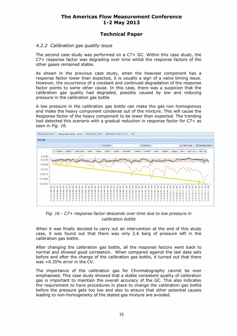
The second case study was performed on a C7+ GC. Within this case study, the C7+ response factor was degrading over time whilst the response factors of the other gases remained stable.
As shown in the previous case study, when the heaviest component has a response factor lower than expected, it is usually a sign of a valve timing issue. However, the occurrence of a constant and continued degradation of the response factor points to some other cause. In this case, there was a suspicion that the calibration gas quality had degraded, possibly caused by low and reducing pressure in the calibration gas bottle
A low pressure in the calibration gas bottle can make the gas non homogenous and make the heavy component condense out of the mixture. This will cause the
Response factor of the heavy component to be lower than expected. The trending tool detected this scenario with a gradual reduction in response factor for C7+ as seen in Fig. 16.
Fig. 16 - C7+ response factor descends over time due to low pressure in
calibration bottle
When it was finally decided to carry out an intervention at the end of this study case, it was found out that there was only 2.6 barg of pressure left in the calibration gas bottle.
After changing the calibration gas bottle, all the response factors went back to
normal and showed good correlation. When compared against the last data sets before and after the change of the calibration gas bottle, it turned out that there was +0.35% error in the CV.
The importance of the calibration gas for Chromatography cannot be over emphasised. This case study showed that a stable consistent quality of calibration gas is important to maintain the overall accuracy of the GC. This also indicates
the requirement to have procedures in place to change the calibration gas bottle before the pressure gets too low and also to ensure that other potential causes leading to non-homogeneity of the stated gas mixture are avoided.
The Americas Flow Measurement Conference
1-2 May 2013
Technical Paper
16
Uncertainty of Working Reference Mixture 4.3
The working reference mixture uncertainty is normally provided in the UKAS certification accompanying the mixture cylinder. In this example the working reference mixture, with its associated uncertainty, is given in Table 3.
Table 3. Working Reference Mixture relative uncertainty
Component WRM (%mol/mol) Absolute
Uncertainty (k=2)
Expanded Relative
Uncertainty (%)
Standard Relative
Uncertainty
Methane 75.605 0.05 0.0661 0.03305
Nitrogen 0.5 0.01 2.0000 1
carbon dioxide 1.784 0.011 0.6166 0.3083
Ethane 12.301 0.08 0.6504 0.3252
Propane 6.938 0.022 0.3171 0.15855
i-butane 0.8926 0.005 0.5602 0.2801
n-butane 1.6218 0.0094 0.5796 0.2898
neo-pentane 0.1026 0.0022 2.1442 1.0721
iso-pentane 0.2259 0.0021 0.9296 0.4648
n-pentane 0.1973 0.0024 1.2164 0.6082
n-hexane 0.0991 0.0017 1.7154 0.8577
Uncertainty from the GC repeatability 4.4
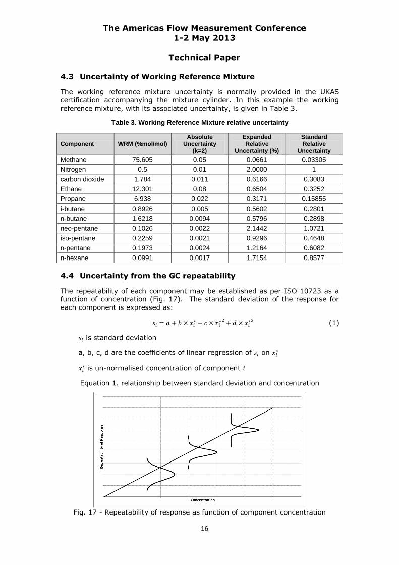
The repeatability of each component may be established as per ISO 10723 as a function of concentration (Fig. 17). The standard deviation of the response for each component is expressed as:
(1)
is standard deviation
a, b, c, d are the coefficients of linear regression of on
is un-normalised concentration of component
Equation 1. relationship between standard deviation and concentration
Fig. 17 - Repeatability of response as function of component concentration
The Americas Flow Measurement Conference
1-2 May 2013
Technical Paper
17
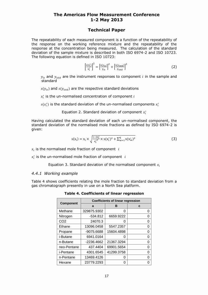
The repeatability of each measured component is a function of the repeatability of
the response on the working reference mixture and the repeatability of the response at the concentration being measured. The calculation of the standard deviation of the sample mixture is described in both ISO 6974-2 and ISO 10723. The following equation is defined in ISO 10723:
[
]
[
]
[
]
(2)
and are the instrument responses to component in the sample and standard
and are the respective standard deviations
is the un-normalised concentration of component
is the standard deviation of the un-normalised components
Equation 2. Standard deviation of component
Having calculated the standard deviation of each un-normalised component, the standard deviation of the normalised mole fractions as defined by ISO 6974-2 is given:
√
∑
(3)
is the normalised mole fraction of component
is the un-normalised mole fraction of component
Equation 3. Standard deviation of the normalised component
4.4.1 Working example
Table 4 shows coefficients relating the mole fraction to standard deviation from a gas chromatograph presently in use on a North Sea platform.
Table 4. Coefficients of linear regression
Component Coefficients of linear regression
a B c
Methane 329875.9302 0 0
Nitrogen -534.812 6659.9222 0
CO2 24070.3 0 0
Ethane 13096.0458 5547.2357 0
Propane -9075.6688 15604.4898 0
i-Butane 6941.0164 0 0
n-Butane -2236.4662 21367.3294 0
neo-Pentane 437.4404 69901.5654 0
i-Pentane 4301.6545 41299.3758 0
n-Pentane 13469.4126 0 0
Hexane 23779.2293 0 0
The Americas Flow Measurement Conference
1-2 May 2013
Technical Paper
18
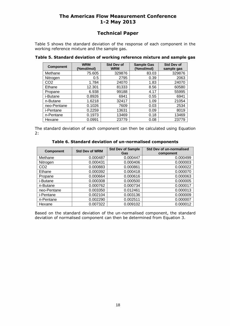
Table 5 shows the standard deviation of the response of each component in the
working reference mixture and the sample gas.
Table 5. Standard deviation of working reference mixture and sample gas
Component WRM
(%mol/mol) Std Dev of
WRM Sample Gas (%mol/mol)
Std Dev of sample gas
Methane 75.605 329876 83.03 329876
Nitrogen 0.5 2795 0.39 2063 CO2 1.784 24070 1.83 24070
Ethane 12.301 81333 8.56 60580
Propane 6.938 99188 4.17 55995
i-Butane 0.8926 6941 0.55 6941
n-Butane 1.6218 32417 1.09 21054
neo-Pentane 0.1026 7609 0.03 2534
i-Pentane 0.2259 13631 0.09 8019
n-Pentane 0.1973 13469 0.18 13469
Hexane 0.0991 23779 0.08 23779
The standard deviation of each component can then be calculated using Equation 2:
Table 6. Standard deviation of un-normalised components
Component Std Dev of WRM Std Dev of Sample
Gas Std Dev of un-normalised
component
Methane 0.000487 0.000447 0.000499
Nitrogen 0.000431 0.000406 0.000003
CO2 0.000883 0.000861 0.000022
Ethane 0.000392 0.000418 0.000070
Propane 0.000664 0.000616 0.000063
i-Butane 0.000308 0.000500 0.000005
n-Butane 0.000762 0.000734 0.000017
neo-Pentane 0.003350 0.012461 0.000013
i-Pentane 0.002104 0.003136 0.000009
n-Pentane 0.002290 0.002511 0.000007
Hexane 0.007322 0.009102 0.000012
Based on the standard deviation of the un-normalised component, the standard deviation of normalised component can then be determined from Equation 3.
The Americas Flow Measurement Conference
1-2 May 2013
Technical Paper
19
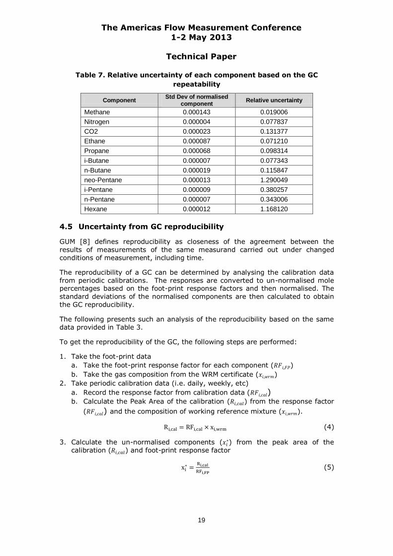
Table 7. Relative uncertainty of each component based on the GC
repeatability
Component Std Dev of normalised
component Relative uncertainty
Methane 0.000143 0.019006
Nitrogen 0.000004 0.077837
CO2 0.000023 0.131377
Ethane 0.000087 0.071210
Propane 0.000068 0.098314
i-Butane 0.000007 0.077343
n-Butane 0.000019 0.115847
neo-Pentane 0.000013 1.290049
i-Pentane 0.000009 0.380257
n-Pentane 0.000007 0.343006
Hexane 0.000012 1.168120
Uncertainty from GC reproducibility 4.5
GUM [8] defines reproducibility as closeness of the agreement between the
results of measurements of the same measurand carried out under changed conditions of measurement, including time.
The reproducibility of a GC can be determined by analysing the calibration data from periodic calibrations. The responses are converted to un-normalised mole percentages based on the foot-print response factors and then normalised. The standard deviations of the normalised components are then calculated to obtain
the GC reproducibility.
The following presents such an analysis of the reproducibility based on the same data provided in Table 3.
To get the reproducibility of the GC, the following steps are performed:
1. Take the foot-print data
a. Take the foot-print response factor for each component ( )
b. Take the gas composition from the WRM certificate ( )
2. Take periodic calibration data (i.e. daily, weekly, etc)
a. Record the response factor from calibration data ( ) b. Calculate the Peak Area of the calibration ( ) from the response factor
( ) and the composition of working reference mixture ( ).
(4)
3. Calculate the un-normalised components ( ) from the peak area of the
calibration ( ) and foot-print response factor
(5)
The Americas Flow Measurement Conference
1-2 May 2013
Technical Paper
20
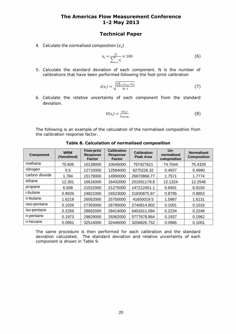
4. Calculate the normalised composition ( )
∑
(6)
5. Calculate the standard deviation of each component. N is the number of calibrations that have been performed following the foot-print calibration
√∑ ̅
(7)
6. Calculate the relative uncertainty of each component from the standard deviation.
(8)
The following is an example of the calculation of the normalised composition from the calibration response factor.
Table 8. Calculation of normalised composition
Component WRM
(%mol/mol)
Foot-print Response
Factor
Calibration Response
Factor
Calibration Peak Area
Un-normalised
composition
Normalised Composition
methane 75.605 10139000 10045000 757427621 74.7044 75.4329
nitrogen 0.5 12710000 12584000 6275226.32 0.4937 0.4990
carbon dioxide 1.784 15179000 14990000 26670868.77 1.7571 1.7774
ethane 12.301 16616000 16432000 201591178.8 12.1324 12.2548
propane 6.938 21522000 21275000 147212451.1 6.8401 6.9150
i-butane 0.8926 24821000 24523000 21830875.87 0.8795 0.8853
n-butane 1.6218 26052000 25750000 41650019.5 1.5987 1.6131
neo-pentane 0.1026 27393000 26785000 2740814.802 0.1001 0.1016
iso-pentane 0.2259 28652000 28414000 6401611.094 0.2234 0.2246
n-pentane 0.1973 29829000 29362000 5777678.864 0.1937 0.1962
n-hexane 0.0991 32514000 32446000 3206826.752 0.0986 0.1001
The same procedure is then performed for each calibration and the standard deviation calculated. The standard deviation and relative uncertainty of each component is shown in Table 9.
The Americas Flow Measurement Conference
1-2 May 2013
Technical Paper
21
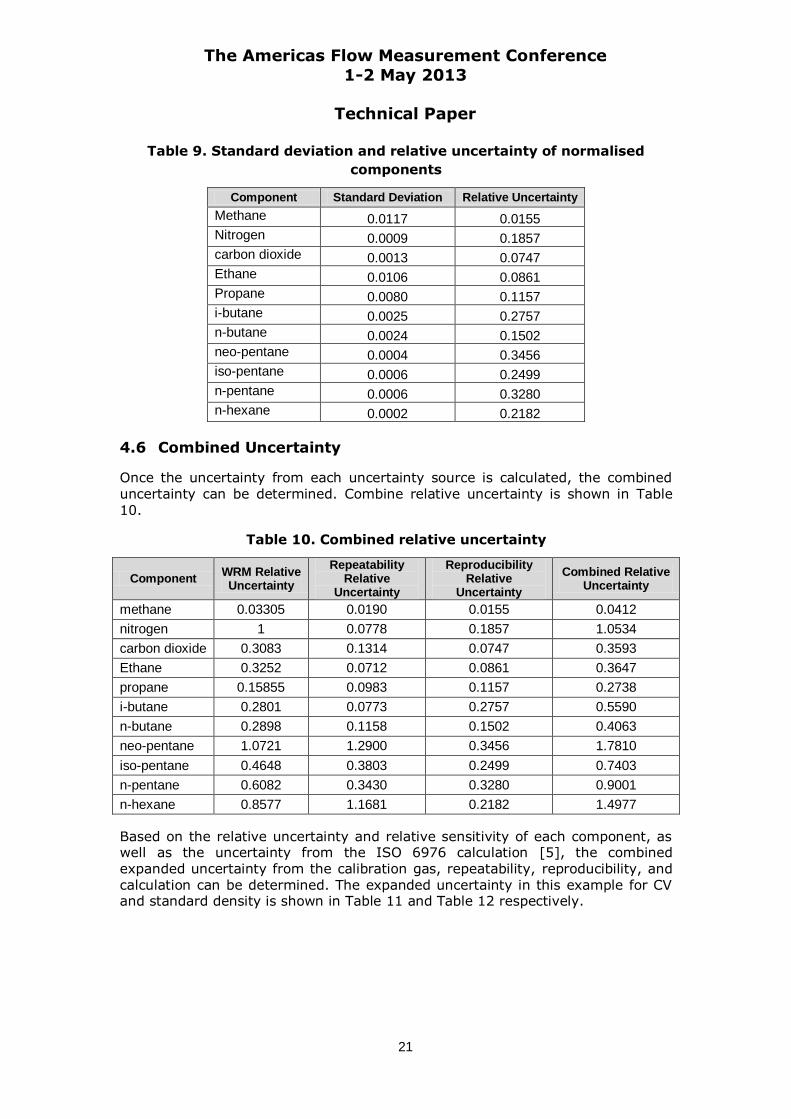
Table 9. Standard deviation and relative uncertainty of normalised
components
Component Standard Deviation Relative Uncertainty
Methane 0.0117 0.0155
Nitrogen 0.0009 0.1857
carbon dioxide 0.0013 0.0747
Ethane 0.0106 0.0861
Propane 0.0080 0.1157
i-butane 0.0025 0.2757
n-butane 0.0024 0.1502
neo-pentane 0.0004 0.3456
iso-pentane 0.0006 0.2499
n-pentane 0.0006 0.3280
n-hexane 0.0002 0.2182
Combined Uncertainty 4.6
Once the uncertainty from each uncertainty source is calculated, the combined uncertainty can be determined. Combine relative uncertainty is shown in Table
10.
Table 10. Combined relative uncertainty
Component WRM Relative Uncertainty
Repeatability Relative
Uncertainty
Reproducibility Relative
Uncertainty
Combined Relative Uncertainty
methane 0.03305 0.0190 0.0155 0.0412
nitrogen 1 0.0778 0.1857 1.0534
carbon dioxide 0.3083 0.1314 0.0747 0.3593
Ethane 0.3252 0.0712 0.0861 0.3647
propane 0.15855 0.0983 0.1157 0.2738
i-butane 0.2801 0.0773 0.2757 0.5590
n-butane 0.2898 0.1158 0.1502 0.4063
neo-pentane 1.0721 1.2900 0.3456 1.7810
iso-pentane 0.4648 0.3803 0.2499 0.7403
n-pentane 0.6082 0.3430 0.3280 0.9001
n-hexane 0.8577 1.1681 0.2182 1.4977
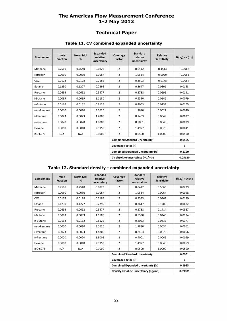
Based on the relative uncertainty and relative sensitivity of each component, as well as the uncertainty from the ISO 6976 calculation [5], the combined expanded uncertainty from the calibration gas, repeatability, reproducibility, and calculation can be determined. The expanded uncertainty in this example for CV and standard density is shown in Table 11 and Table 12 respectively.
The Americas Flow Measurement Conference
1-2 May 2013
Technical Paper
22
Table 11. CV combined expanded uncertainty
Component mole
Fraction Norm Mol
%
Expanded relative
uncertainty
Coverage factor
Standard relative
uncertainty
Relative Sensitivity
Methane 0.7561 0.7540 0.0823 2 0.0412 -0.1513 -0.0062
Nitrogen 0.0050 0.0050 2.1067 2 1.0534 -0.0050 -0.0053
CO2 0.0178 0.0178 0.7185 2 0.3593 -0.0178 -0.0064
Ethane 0.1230 0.1227 0.7295 2 0.3647 0.0501 0.0183
Propane 0.0694 0.0692 0.5477 2 0.2738 0.0696 0.0191
i-Butane 0.0089 0.0089 1.1180 2 0.5590 0.0142 0.0079
n-Butane 0.0162 0.0162 0.8125 2 0.4063 0.0259 0.0105
neo-Pentane 0.0010 0.0010 3.5620 2 1.7810 0.0022 0.0040
i-Pentane 0.0023 0.0023 1.4805 2 0.7403 0.0049 0.0037
n-Pentane 0.0020 0.0020 1.8003 2 0.9001 0.0043 0.0039
Hexane 0.0010 0.0010 2.9953 2 1.4977 0.0028 0.0041
ISO 6976 N/A N/A 0.1000 2 0.0500 1.0000 0.0500
Combined Standard Uncertainty 0.0595
Coverage Factor (k) 2
Combined Expanded Uncertainty (%) 0.1190
CV absolute uncertainty (MJ/m3) 0.05620
Table 12. Standard density - combined expanded uncertainty
Component mole
Fraction Norm Mol
%
Expanded relative
uncertainty
Coverage factor
Standard relative
uncertainty
Relative Sensitivity
Methane 0.7561 0.7540 0.0823 2 0.0412 0.5563 0.0229
Nitrogen 0.0050 0.0050 2.1067 2 1.0534 0.0064 0.0068
CO2 0.0178 0.0178 0.7185 2 0.3593 0.0361 0.0130
Ethane 0.1230 0.1227 0.7295 2 0.3647 0.1706 0.0622
Propane 0.0694 0.0692 0.5477 2 0.2738 0.1414 0.0387
i-Butane 0.0089 0.0089 1.1180 2 0.5590 0.0240 0.0134
n-Butane 0.0162 0.0162 0.8125 2 0.4063 0.0436 0.0177
neo-Pentane 0.0010 0.0010 3.5620 2 1.7810 0.0034 0.0061
i-Pentane 0.0023 0.0023 1.4805 2 0.7403 0.0075 0.0056
n-Pentane 0.0020 0.0020 1.8003 2 0.9001 0.0066 0.0059
Hexane 0.0010 0.0010 2.9953 2 1.4977 0.0040 0.0059
ISO 6976 N/A N/A 0.1000 2 0.0500 1.0000 0.0500
Combined Standard Uncertainty 0.0961
Coverage Factor (k) 2
Combined Expanded Uncertainty (%) 0.1923
Density absolute uncertainty (Kg/m3) 0.09081
The Americas Flow Measurement Conference
1-2 May 2013
Technical Paper
23
Systematic Error 4.7
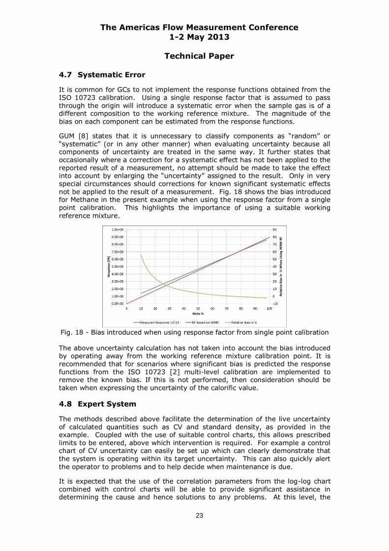
It is common for GCs to not implement the response functions obtained from the ISO 10723 calibration. Using a single response factor that is assumed to pass through the origin will introduce a systematic error when the sample gas is of a different composition to the working reference mixture. The magnitude of the bias on each component can be estimated from the response functions.
GUM [8] states that it is unnecessary to classify components as “random” or “systematic” (or in any other manner) when evaluating uncertainty because all components of uncertainty are treated in the same way. It further states that occasionally where a correction for a systematic effect has not been applied to the reported result of a measurement, no attempt should be made to take the effect into account by enlarging the “uncertainty” assigned to the result. Only in very special circumstances should corrections for known significant systematic effects
not be applied to the result of a measurement. Fig. 18 shows the bias introduced for Methane in the present example when using the response factor from a single point calibration. This highlights the importance of using a suitable working reference mixture.
Fig. 18 - Bias introduced when using response factor from single point calibration
The above uncertainty calculation has not taken into account the bias introduced by operating away from the working reference mixture calibration point. It is recommended that for scenarios where significant bias is predicted the response functions from the ISO 10723 [2] multi-level calibration are implemented to remove the known bias. If this is not performed, then consideration should be taken when expressing the uncertainty of the calorific value.
Expert System 4.8
The methods described above facilitate the determination of the live uncertainty of calculated quantities such as CV and standard density, as provided in the example. Coupled with the use of suitable control charts, this allows prescribed limits to be entered, above which intervention is required. For example a control chart of CV uncertainty can easily be set up which can clearly demonstrate that the system is operating within its target uncertainty. This can also quickly alert
the operator to problems and to help decide when maintenance is due.
It is expected that the use of the correlation parameters from the log-log chart combined with control charts will be able to provide significant assistance in determining the cause and hence solutions to any problems. At this level, the
The Americas Flow Measurement Conference
1-2 May 2013
Technical Paper
24
method is approaching that on an expert system, which may loosely be defined
as a computer system that emulates the decision-making ability of a human expert.
5 CONCLUSION
This paper has described methods that may be used for monitoring the performance of gas chromatographs. It is important to ensure the initial health of
the GC to avoid systematic error. Once it is determined that the GC is healthy, data commonly available from the WRM certificate, ISO 10723 multilevel calibrations, and long term reproducibility can be utilised to provide live uncertainty calculations giving assurance that GC performance is within prescribed limits throughout the year.
The principle is equally applicable to calculations such as line density based on compressibility from AGA 8 [1] and any other compositional based calculations. The application of the method is expected to help to maintain the GC within its specified requirements throughout the year.
6 NOTATION
GC Gas Chromatograph CBM Conditional Based Monitoring CV Calorific Value EUETS European Union Emission
Trading Scheme k Coverage factor Coefficients of linear
regression of on
standard deviation Un-normalised concentration of
component Normalised concentration of
component
Standard deviation of the un-
normalised components
Instrument responses to component in the sample
Instrument responses to component in the standard
Standard deviations of
component in the sample Standard deviations of
component in the standard Standard deviation of the
normalised mole fractions Number of components
analysed CRM Certified Reference Mixture.
Mixture which is used for the determination of the response curves of the measuring system.
WRM Working Reference Mixture.
Mixture which is used as a working standard for regular calibration of the measuring system
GUM Guide to the expression of uncertainty in measurement
Foot-print response factor for
component
Calibration data response
factor for component Mole fraction of component in
WRM
Peak Area from calibration of
component N Number of calibrations that
have been performed following the foot-print calibration
Relative sensitivity coefficient
of component mole fraction Relative uncertainty of
component mole fraction mmscfd Million standard cubic feet per
day MMBTU Million British Thermal Unit MJ Mega Joules GJ Giga Joules

The Americas Flow Measurement Conference
1-2 May 2013
Technical Paper
25
7 REFERENCES
[1] AGA 8. Compressibility and supercompressibility of natural gas and other related hydrocarbon gases (2nd printing july 1994). AGA, 1992.
[2] BS EN ISO 10723. Natural gas - performance evaluation for on-line analytical systems. BS EN ISO, 2002.
[3] BS EN ISO 6974-5. Natural gas - Determination of composition with defined uncertainty by gas chromatography - Part 5: Determination of nitrogen, carbon dioxide and C1 to C5 and C6+ hydrocarbons for a laboratory and on-line process application using three columns. BS EN ISO, 2001.
[4] Commission Decision 2007 589 EC. Commission decision. establishing guidelines for the monitoring and reporting of greenhouse gas emissions pursuant to directive 2003/87/ec of the european parliament and of the council. Official Journal of the European Union, May 2007.
[5] ISO 6976. Natural Gas - Calculation of calorific values, density, relative density and Wobbe index from composition. ISO, (Technical Corrigendum 3), 1996.
[6] ISO/IEC 17025. General requirements for the competence of testing and calibration laboratories. ISO, 2005.
[7] Library4Science.com. Retention time. [Online], 2008. Available: http://www.chromatography-online.org/topics/retention/time.html.
[8] OIML G 1-100. Evaluation of measurement data - guide to the expression of
uncertainty in measurement. OIML, 2010.
[9] Anwar Sutan, Charles Johnson, and Jason Laidlaw. Three columns gas chromatograph analysis using correlation between component’s molecular weight and its response factor. North Sea Flow Measurement Workshop, 2009.
[10] Ycharts. Henry hub natural gas spot price. [Online], 2013. Available:
http://ycharts.com/indicators/natural_gas_spot_price.