Embed Size (px)
Citation preview
RETIREMENT SECURITY
Income and Wealth Disparities Continue through Old Age
Report to Ranking Member, Committee on the Budget, U.S. Senate
August 2019
GAO-19-587
United States Government Accountability Office
______________________________________ United States Government Accountability Office
August 2019
RETIREMENT SECURITY Income and Wealth Disparities Continue through Old Age
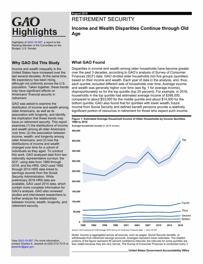
What GAO Found Disparities in income and wealth among older households have become greater over the past 3 decades, according to GAO’s analysis of Survey of Consumer Finances (SCF) data. GAO divided older households into five groups (quintiles) based on their income and wealth. Each year of data in the analysis, and, thus, each quintile, included different sets of households over time. Average income and wealth was generally higher over time (see fig. 1 for average income), disproportionately so for the top quintile (top 20 percent). For example, in 2016, households in the top quintile had estimated average income of $398,000, compared to about $53,000 for the middle quintile and about $14,000 for the bottom quintile. GAO also found that for quintiles with lower wealth, future income from Social Security and defined benefit pensions provide a relatively significant portion of resources in retirement for those who expect such income.
Figure 1: Estimated Average Household Income of Older Households by Income Quintiles, 1989 to 2016
Notes: Income is aggregated across all sources, such as wages, Social Security benefits, or withdrawals from retirement savings accounts. Averages represent mean estimates. The shaded portions of the figure represent 95 percent confidence intervals; the intervals for some quintiles are less visible because they are very narrow. The Survey of Consumer Finances is conducted every 3
Why GAO Did This Study Income and wealth inequality in the United States have increased over the last several decades. At the same time, life expectancy has been rising, although not uniformly across the U.S. population. Taken together, these trends may have significant effects on Americans’ financial security in retirement.
GAO was asked to examine the distribution of income and wealth among older Americans, as well as its association with longevity, and identify the implication that these trends may have on retirement security. This report examines (1) the distributions of income and wealth among all older Americans over time; (2) the association between income, wealth, and longevity among older Americans; and (3) how the distributions of income and wealth changed over time for a cohort of individuals as they aged. To conduct this work, GAO analyzed data from two nationally representative surveys: the SCF, using data from 1989 through 2016, and the HRS. GAO used 1992 through 2014 HRS data linked to earnings records from the Social Security Administration. While preliminary 2016 HRS data are available, GAO used 2014 data, which contain more complete information for GAO’s analysis. GAO also reviewed studies and interviewed researchers to further analyze the relationships between income, wealth, longevity, and retirement security.
View GAO-19-587. For more information, contact Charles A. Jeszeck at (202) 512-7215 or [email protected].
Highlights of GAO-19-587, a report to the Ranking Member of the Committee on the Budget, U.S. Senate
______________________________________ United States Government Accountability Office
years. Older households are those where the survey respondents or any spouses or partners were aged 55 or older in the year of the survey. GAO ranked these households by their income and broke them into five equally sized groups, or quintiles. Each year of data in our analysis, and, therefore, each quintile included different sets of households over time.
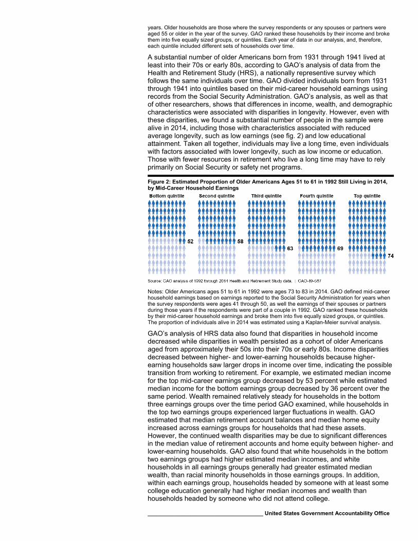
A substantial number of older Americans born from 1931 through 1941 lived at least into their 70s or early 80s, according to GAO’s analysis of data from the Health and Retirement Study (HRS), a nationally representive survey which follows the same individuals over time. GAO divided individuals born from 1931 through 1941 into quintiles based on their mid-career household earnings using records from the Social Security Administration. GAO’s analysis, as well as that of other researchers, shows that differences in income, wealth, and demographic characteristics were associated with disparities in longevity. However, even with these disparities, we found a substantial number of people in the sample were alive in 2014, including those with characteristics associated with reduced average longevity, such as low earnings (see fig. 2) and low educational attainment. Taken all together, individuals may live a long time, even individuals with factors associated with lower longevity, such as low income or education. Those with fewer resources in retirement who live a long time may have to rely primarily on Social Security or safety net programs.
Figure 2: Estimated Proportion of Older Americans Ages 51 to 61 in 1992 Still Living in 2014, by Mid-Career Household Earnings
Notes: Older Americans ages 51 to 61 in 1992 were ages 73 to 83 in 2014. GAO defined mid-career household earnings based on earnings reported to the Social Security Administration for years when the survey respondents were ages 41 through 50, as well the earnings of their spouses or partners during those years if the respondents were part of a couple in 1992. GAO ranked these households by their mid-career household earnings and broke them into five equally sized groups, or quintiles. The proportion of individuals alive in 2014 was estimated using a Kaplan-Meier survival analysis.
GAO’s analysis of HRS data also found that disparities in household income decreased while disparities in wealth persisted as a cohort of older Americans aged from approximately their 50s into their 70s or early 80s. Income disparities decreased between higher- and lower-earning households because higher-earning households saw larger drops in income over time, indicating the possible transition from working to retirement. For example, we estimated median income for the top mid-career earnings group decreased by 53 percent while estimated median income for the bottom earnings group decreased by 36 percent over the same period. Wealth remained relatively steady for households in the bottom three earnings groups over the time period GAO examined, while households in the top two earnings groups experienced larger fluctuations in wealth. GAO estimated that median retirement account balances and median home equity increased across earnings groups for households that had these assets. However, the continued wealth disparities may be due to significant differences in the median value of retirement accounts and home equity between higher- and lower-earning households. GAO also found that white households in the bottom two earnings groups had higher estimated median incomes, and white households in all earnings groups generally had greater estimated median wealth, than racial minority households in those earnings groups. In addition, within each earnings group, households headed by someone with at least some college education generally had higher median incomes and wealth than households headed by someone who did not attend college.
Page i GAO-19-587 Income and Wealth of Older Americans
Letter 1
Background 5 Disparities in Income and Wealth Increased Among Older
Households Even As More Households Had Retirement Accounts 9
A Substantial Number of Older Americans Are Living Into Their Seventies or Early Eighties, Which May Have Implications for Retirement Security 34
While Income Disparities Declined As a Cohort of Older Americans Aged and Worked Less, Disparities in Wealth Persisted 41
Agency Comments 54
Appendix I Objectives, Scope, and Methodology 55
Appendix II Financial and Demographic Characteristics across the Wealth Distribution 77
Appendix III Additional Data Tables 83
Appendix IV Additional Survival Analysis Results 103
Appendix V 2014 Population in the Health and Retirement Study (HRS) 112
Appendix VI Estimated Income and Wealth for War Babies Cohort 114
Appendix VII GAO Contact and Staff Acknowledgments 117
Contents
Page ii GAO-19-587 Income and Wealth of Older Americans
Bibliography 118
Related GAO Products 122
Tables
Table 1: Characteristics of Households in the Health and Retirement Study Interviewed in Both 1992 and 2014 42
Table 2: Number of Respondents Included in Survey of Consumer Finances Interviews Compared to Number of Respondents in Public Dataset 58
Table 3: Health and Retirement Study (HRS) Cohorts 67 Table 4: Confidence Intervals for Estimates Shown in Figure 5 83 Table 5: Confidence Intervals for Estimates Shown in Figure 6 86 Table 6: Confidence Intervals for Estimated Percentage of Older
Households with Retirement Account Balances by Amount in 2016, as shown in Figure 10 91
Table 7: Estimated Median Household Income for Individuals Born in 1931-1941 and Their Spouses or Partners, as They Aged, by Mid-Career Earnings Level and Race and Ethnicity 94
Table 8: Estimated Median Household Wealth for Individuals Born in 1931-1941 and Their Spouses or Partners, as They Aged, by Mid-Career Earnings Level and Race and Ethnicity 96
Table 9: Estimated Median Household Income for Individuals Born in 1931-1941 and Their Spouses or Partners, as They Aged, by Mid-Career Earnings Level and Education 98
Table 10: Estimated Median Household Wealth for Individuals Born in 1931-1941 and Their Spouses or Partners, as They Aged, by Mid-Career Earnings Level and Education 100
Table 11: Proportion of Those Ages 51 to 61 in 1992 Living to Ages 73 to 83 in 2014, By Mid-Career Household Earnings 103
Table 12: Proportion of Those Ages 51 to 61 in 1992 Living to Ages 73 to 83 in 2014, By Health and Earnings Categories 104
Table 13: Proportion of Those Ages 51 to 61 in 1992 Living to Ages 73 to 83 in 2014, By Race and Ethnicity 105
Page iii GAO-19-587 Income and Wealth of Older Americans
Table 14: Proportion of Those Ages 51 to 61 in 1992 Living to Ages 73 to 83 in 2014, By Household Wealth in 1992 105
Table 15: Proportion of Those Ages 51 to 61 in 1992 Living to Ages 73 to 83 in 2014, By Education Level 106
Table 16: Proportion of Those Ages 51 to 61 in 1992 Living to Ages 73 to 83 in 2014, By Gender 107
Table 17: Proportion of Those Ages 51 to 61 in 1992 Living to Ages 73 to 83 in 2014, By Self-Reported Health Status in 1992 108
Table 18: Estimated Hazard Ratios of Living to Ages 73 to 83 in 2014, for Those Ages 51 to 61 in 1992, By Mid-Career Household Earnings and Demographic Characteristics 109
Table 19: Estimated Hazard Ratios of Living to Ages 73 to 83 in 2014, for Those Ages 51 to 61 in 1992, By Household Wealth in 1992 and Demographic Characteristics 110
Table 20: Race and Ethnicity of Household Head by Mid-Career Earnings Quintile in 2014 112
Table 21: Education Level of Household Head by Mid-Career Earnings Quintile in 2014 112
Table 22: Household Type by Mid-Career Earnings Quintile in 2014 113
Figures
Figure 1: Estimated Average and Median Income of Older Households by Income Quintiles, 1989 to 2016 11
Figure 2: Estimated Average and Median Wealth of Older Households by Wealth Quintiles, 1989 to 2016 13
Figure 3: Estimated Average and Median Income of Older Households in the Top 1 Percent of the Income Distribution, 1989 to 2016 15
Figure 4: Estimated Average and Median Wealth of Older Households in the Top 1 Percent of the Wealth Distribution, 1989 to 2016 16
Figure 5: Estimated Average Wealth Plus Present Value of Future Income of Older Households Expecting Future Income from Social Security but Not a Pension, 1989 to 2016 19
Figure 6: Estimated Average Wealth Plus Present Value of Future Income of Older Households Expecting Future Income from Social Security and Pensions, 1989 to 2016 21
Page iv GAO-19-587 Income and Wealth of Older Americans
Figure 7: Estimated Wealth of Older Households in the Middle Quintile of the Wealth Distribution by Race and Ethnicity, Education, and Marital Status, 1989 to 2016 24
Figure 8: Estimated Wealth of Older Households in the Top 20 Percent of the Wealth Distribution by Race and Ethnicity, Education, and Marital Status, 1989 to 2016 26
Figure 9: Estimated Percentage of Older Households with Selected Retirement Resources by Wealth Quintiles, 1989 to 2016 29
Figure 10: Estimated Distribution of Average Retirement Account Balances among Older Households by Wealth Quintiles, 2016 30
Figure 11: Estimated Percentage of Older Households with Selected Assets by Wealth Quintiles, 1989 to 2016 31
Figure 12: Estimated Proportion of Older Americans Ages 51 to 61 in 1992 Still Living in 2014, by Mid-Career Household Earnings 36
Figure 13: Estimated Proportion of Those Ages 51 to 61 in 1992 Still Living in 2014, Across Earnings and Education Scenarios 40
Figure 14: Estimated Median Household Income for Individuals Born in 1931-1941 and Their Spouses or Partners, as They Aged, by Mid-Career Earnings Level 44
Figure 15: Estimated Median Household Wealth for Individuals Born in 1931-1941 and Their Spouses or Partners, as They Aged, by Mid-Career Earnings Level 47
Figure 16: Estimated Median Retirement Account Balances for Households with Retirement Accounts as Individuals Born in 1931-1941 and Their Spouses or Partners Aged, by Mid-Career Earnings Level 49
Figure 17: Estimated Median Value of Home Equity for Households with Home Equity, as Individuals Born in 1931-1941 and Their Spouses or Partners Aged, by Mid-Career Earnings Level 51
Figure 18: Estimated Median Household Income for Individuals Born in 1942-1947 and Their Spouses or Partners, As They Aged by Mid-Career Earnings Level 114
Figure 19: Estimated Median Household Wealth for Individuals Born in 1942-1947 and Their Spouses or Partners, As They Aged, by Mid-Career Earnings Level 115
Page v GAO-19-587 Income and Wealth of Older Americans
Abbreviations DB defined benefit DC defined contribution ERISA Employee Retirement Income Security Act of 1974 FA Financial Accounts of the United States Federal Reserve Board of Governors of the Federal Reserve System HRS Health and Retirement Study IRA individual retirement account IRC Internal Revenue Code SCF Survey of Consumer Finances SSA Social Security Administration
This is a work of the U.S. government and is not subject to copyright protection in the United States. The published product may be reproduced and distributed in its entirety without further permission from GAO. However, because this work may contain copyrighted images or other material, permission from the copyright holder may be necessary if you wish to reproduce this material separately.
Page 1 GAO-19-587 Income and Wealth of Older Americans
441 G St. N.W. Washington, DC 20548
August 9, 2019
The Honorable Bernard Sanders Ranking Member Committee on the Budget United States Senate
Dear Senator Sanders:
Income and wealth inequality in the United States have increased over several decades. While income inequality in the United States was relatively stable from the 1940s to the 1970s, since then wage growth at the top of the income distribution has outpaced the rest of the distribution, and inequality has risen. Wealth has become increasingly concentrated as well. By 2013, those families in the top 10 percent of the wealth distribution held 76 percent of the wealth held by all families in the United States.1 Inequality among older Americans, specifically, is an area of concern for some policy makers and researchers, particularly given trends related to the U.S. retirement system over this same time period. For example, average life expectancy has increased. This is a positive development, but it also requires more planning and saving to support more years in retirement. Further, income, wealth, and longevity are each interconnected with one another. For example, life expectancy has not increased uniformly across all income groups, and people who have lower incomes tend to have shorter lives than those with higher incomes. There is concern among some researchers and policy makers that disparities in income, wealth, and life expectancy may be indicative of potential problems for many Americans’ financial security in retirement.
You asked us to examine the distribution of income and wealth among older Americans and identify the implication of these trends, along with associations with longevity, on retirement security. This report examines (1) the distributions of income and wealth among all older Americans over time; (2) the association between income, wealth, and longevity among older Americans; and (3) how the distributions of income and wealth have changed over time for a cohort of individuals as they aged.
1Congressional Budget Office, Trends in Family Wealth, 1989 to 2013, Report 51846 (Washington, D.C.: August 2016).
Letter
Page 2 GAO-19-587 Income and Wealth of Older Americans
To examine the distribution of income and wealth among all older Americans over time, we used 1989 through 2016 data from the Survey of Consumer Finances, a triennial, cross-sectional survey produced by the Board of Governors of the Federal Reserve System (Federal Reserve). A different sample of households was used for each year in our analysis. These data allow for comparison of the experiences of same-age households at different points in time. We chose to look at household-level resources because couples may pool their economic resources and the SCF asks some of its questions about resources for households. For each survey year, we examined the distribution of income and wealth for older households as a whole and by household heads’ race and ethnicity, marital status and gender, and education level. We defined older households as those in which the household head or any spouses or partners were aged 55 or older. We also analyzed the percentage of households that held various sources of income and wealth and the amounts of such sources across the income and wealth distributions.
Lastly, we used these data, supplemented by data from the Financial Accounts of the United States–another data source published by the Federal Reserve–to estimate the present value of future income expected from defined benefit (DB) pension plans and Social Security. To do so, we followed methods developed by economists at the Federal Reserve, with some modifications to the Social Security methods, in particular, to meet the purposes of our analysis.2 Alternative methods of analyzing distributional disparities in retirement security exist. For example, one option would be to evaluate how future monthly income from Social Security and DB pensions would be expected to affect retirement security, perhaps by assessing how the standard of living for workers would be expected to change. Additionally, disparities in health in adulthood could contribute to subsequent disparities in income and wealth at older ages. However, for our analysis of how income and wealth are distributed across older Americans over time, it was useful to estimate the present value of Social Security and DB pensions so we could compare the value of these sources to retirement account balances. In
2The Federal Reserve economists continue to refine their methodology, and we relied on recently available papers as a starting point for our analysis. For more on the Federal Reserve economists methods, see Sebastian Devlin-Foltz, Alice Henriques, and John Sabelhaus, “Is the U.S. Retirement System Contributing to Rising Wealth Inequality?” The Russell Sage Foundation Journal of the Social Sciences, vol. 2 no. 6 (2016). For more on the modifications we made, see appendix I.
Page 3 GAO-19-587 Income and Wealth of Older Americans
addition, the SCF does not include sufficient data on health to consider its role in income and wealth disparities for this part of our analysis.
To examine the association between income, wealth, and longevity among a cohort of older Americans, we used 1992 through 2014 data from the Health and Retirement Study (HRS), a nationally representative, longitudinal survey that follows the same set of Americans from their 50s through the remainder of their lives. Use of a longitudinal survey allows us to follow changes for specific individuals as they age. We analyzed data for the cohort of individuals born from 1931 through 1941.3 We identified the distribution of income across these individuals by constructing a measure of mid-career earnings. This measure was constructed at the household level and was based on the household’s average annual reported earnings when the household head was aged 41 to 50. Household earnings data came from administrative records from the Social Security Administration linked to survey responses.4
We then analyzed how the longevity of these individuals varied across mid-career household earnings and demographic characteristics, such as race and education level, using a technique called survival analysis. We were able to measure deaths over a period of 22 years (1992 through 2014). Every 2 years, the HRS attempted to measure whether the original respondents were still alive, but these longevity data were incomplete because some of the original respondents declined to participate in later waves of the survey. Once these respondents left the survey, their actual longevity could not be followed. Survival analysis accounts for survey respondents with complete or incomplete longevity data and allowed us to estimate the chance of death by any given time in the observation period. Most importantly, our analysis assumed actual longevity from 1992 to 2014 of the individuals in our analysis did not have a systematic relationship with whether the original HRS respondents continued to participate in the study except that leaving the study implied a later death. We believe this assumption to be reasonable for the purpose of our analysis for two reasons. First, a small percentage (8 percent) of the original respondents dropped out of the survey, so that the impact of any longevity differences among the population who dropped out would likely 3The HRS program refers to those born from 1931 through 1941 as its core HRS cohort or its original cohort. 4This measure of earnings provides a relatively stable indicator of the household’s labor market experience, compared to using a single year of earnings, which could be unusually high or low. See appendix I for additional details.
Page 4 GAO-19-587 Income and Wealth of Older Americans
have been small. Second, while some baseline characteristics of respondents do appear correlated with non-response over time, the population that dropped out of the study does not appear to vary significantly from those completing each wave, except for race and ethnicity. We conducted this analysis, at the individual level, for HRS respondents in 1992, and any spouses or partners also born in 1931 through 1941.
We also used the HRS data and the mid-career household earnings measure to compare trends in the distributions of income and wealth, at the household level, as the cohort aged. We restricted this analysis to survey respondents (“household heads”), or any spouses or partners as of 1992, who were still alive in 2014 to ensure we followed the same group of people throughout our analysis. This analysis included an examination of trends by demographic characteristics and by specific sources of income and wealth.
For the purposes of our analysis, we defined wealth to be a household’s net worth—that is, total assets minus total debt. Net worth is a measure often used by researchers studying retirement security. As mentioned above in our summary of how we examined the distribution of income and wealth over time, older Americans may also have other future retirement resources, not included in net worth, such as the present value of future income expected from defined benefit (DB) pension plans and Social Security. For all three questions, we supplemented analyses with expert interviews and a literature review to provide greater insight. We specifically identified researchers’ explanations and theories about the relationships between inequality and longevity, health status, gender, race and ethnicity, or education.
For all of the datasets used in our study, we reviewed documentation, interviewed or obtained information from officials responsible for the data, and tested the data for anomalies. We determined that these data are sufficiently reliable for the purposes of this report. To provide additional context on the relationships among income, wealth, longevity, and retirement security, we reviewed 29 studies. The bibliography at the end of this report lists these studies, as well as other recent studies, that informed this report. We also reviewed relevant federal laws and regulations. See appendix I for more detailed information about our scope and methodology.
We conducted this performance audit from August 2017 to August 2019 in accordance with generally accepted government auditing standards.
Page 5 GAO-19-587 Income and Wealth of Older Americans
Those standards require that we plan and perform the audit to obtain sufficient, appropriate evidence to provide a reasonable basis for our findings and conclusions based on our audit objectives. We believe that the evidence obtained provides a reasonable basis for our findings and conclusions based on our audit objectives.
Many older Americans are retired and rely on different parts of the U.S. retirement system for their financial security. The U.S. retirement system is often described as being composed of Social Security, employer-sponsored pensions and retirement savings plans, and individual savings. In addition, older Americans may work past traditional retirement ages or phase into retirement.
Social Security’s Old-Age and Survivors Insurance program is the foundation of the U.S. retirement system and provides benefits to retired workers, their families, and survivors of deceased workers. In 2018, about 53 million retirees and their families received $844.9 billion in Social Security retirement benefits, according to the Social Security Administration.5 However, Social Security is facing financial difficulties that, if not addressed, will affect its long-term stability. If no changes are made, current projections indicate that by 2034, the retirement program Trust Fund will only be sufficient to pay 77 percent of scheduled benefits.6
Employer-sponsored pensions include DB plans, which generally promise to offer a monthly payment to retirees for life. Employers also sponsor defined contribution (DC) plans, such as 401(k)s, in which individuals accumulate tax-advantaged retirement savings in an individual account based on employee and/or employer contributions, and the investment returns (gains and losses) earned on the account. Participants in both DB and DC plans receive certain tax preferences provided the plans comply with requirements outlined in the Internal Revenue Code (IRC). For fiscal year 2018, estimated tax expenditures related to retirement plans and
5The Board of Trustees, The 2019 Annual Report of the Board of Trustees of the Federal Old-Age and Survivors Insurance and Federal Disability Insurance Trust Funds (Washington, D.C.: April 22, 2019). 6Ibid.
Background
Retirement Resources
Page 6 GAO-19-587 Income and Wealth of Older Americans
savings amounted to about $188 billion.7 The Employee Retirement Income Security Act of 1974 (ERISA) outlines minimum standards and requirements that must be met by most private sector employer-sponsored retirement plans; it does not, however, require any employer to establish, or continue to maintain, a retirement plan. Assets rolled over from employer-sponsored DC plans when individuals change jobs or retire are the primary source of funding for individual retirement accounts (IRAs). Over the past 40 years, private sector employers have increasingly moved from offering DB plans to offering DC plans. While DC plans offer more portability, some financial risks—such as poor investment returns, decreases in interest rates, and increases in longevity—have shifted from the employer to the employee, with important implications for individuals’ retirement planning and security.8
Individual savings are any other non-retirement plan savings and investments. Home equity is an important asset for many households. Other sources of savings or wealth may include amounts saved from income or wages, contributions to accounts outside of a retirement plan, non-retirement financial wealth that is inherited or accumulated over time, and equity from other tangible assets such as vehicles.
Defining Resources in Retirement • Wealth: For analyses in this report, we defined wealth as net worth, i.e., assets
minus debt. Assets could be financial (e.g., savings accounts, stocks, bonds, retirement accounts) or nonfinancial (e.g., the value of any houses or vehicles). Retirement accounts include defined contribution plans, such as a 401(k), or individual retirement account (IRA)s. Net worth is a measure often used by researchers studying retirement security.
7Office of Management and Budget, Analytical Perspectives, Budget of the U.S. Government, Fiscal Year 2020 (Washington, D.C.: 2019). This total includes estimates for deferrals for contributions to DB plans, DC plans, and other plans covering partners and sole proprietors, individual retirement accounts, and certain retirement saving tax credits. This estimated total, which is based on provisions of federal tax law enacted through July 1, 2018, is measured as the tax revenue that the government does not currently collect on contributions and investment earnings, offset by the taxes paid by those who are currently receiving retirement benefits. Summing tax expenditure estimates is useful for gauging the general magnitude of revenue forgone through provisions of the tax code, but does not take into account interactions among individual provisions. Revenue loss estimates do not necessarily represent the amount of revenue that would be gained from repealing a tax expenditure, because repeal would probably change taxpayer behavior in some way that would affect revenue. 8For more discussion about the key characteristics of DC and DB plans, see GAO, The Nation’s Retirement System: A Comprehensive Re-evaluation Is Needed to Better Promote Future Retirement Security, GAO-18-111SP (Washington, D.C.: Oct. 18, 2017).
Page 7 GAO-19-587 Income and Wealth of Older Americans
• Present value of future income from Social Security and defined benefit pensions: Older Americans may also have other future retirement resources, not included in net worth, such as the present value of benefits expected from defined benefit (DB) pension plans and Social Security. These present value estimates could be included in a broader definition of economic resources or wealth, and we were able to produce estimates of these additional retirement resources to supplement our analysis of the distribution of income and wealth among older Americans over time. While all estimates produced using survey data are subject to some uncertainty, our present value estimates for these additional retirement resources are also subject to additional uncertainty that arises from using another data source—the Financial Accounts of the United States—to create a measure of aggregate defined benefit entitlements; having limited information about lifetime earnings in the Survey of Consumer Finances; and making assumptions about life expectancy, real discount rates, and retirement ages, which are unlikely to hold for all households. Data limitations prevented us from producing this broader measure of retirement resources for our analysis examining the distributions of income and wealth as a cohort of older Americans aged.
• Income: For analyses in this report, we defined household income as the sum of income across all sources, including wages and salaries, Social Security benefits, traditional pension benefits from defined benefit plans, withdrawals from retirement accounts, and income from any other sources, such as interest on financial assets or benefits from social safety net programs such as the Supplemental Nutrition Assistance Program (SNAP).
See appendix I for more information on our definitions and the methods used to produce estimates of wealth, the present value of future income expected from Social Security and defined benefit plans, and income.
Source: GAO analysis. | GAO-19-587
Older Americans may also have wages or salaries from working longer as they transition to retirement. According to data from the Bureau of Labor Statistics, more older Americans are working. From 1989—the earliest starting year for our analyses—to 2018, the labor force participation rate for Americans aged 55 or older increased from 30 percent to 40 percent. In addition, some older Americans may receive income from financial assets, such as interest or dividends, and from other benefit programs, such as Social Security Disability Insurance.
The number of older Americans is increasing faster than the population as a whole. In 1990, about 52 million, or around 1 in 5, people in the United States were aged 55 or older. By 2030, that number is expected to be about 112 million, or around 1 in 3. The aging of the baby boomers—that is, people born between 1946 and 1964—as well as increasing longevity and lower fertility have contributed to this trend. The oldest baby boomers turned 55 in 2001 and the youngest are turning 55 this year. In addition, average life expectancy for those ages 65 or older has
Increases in the Number of Older Americans
Page 8 GAO-19-587 Income and Wealth of Older Americans
increased significantly over the past century and is projected to continue to increase.9 For example, a man turning 65 in 2030 is expected to live, on average, to age 85.0, an additional 5.3 years compared to a man who turned 65 in 1980, who was expected to live, on average, to age 79.7. A woman turning 65 in 2030 is expected to live, on average, to age 87.3, an additional 3.5 years compared to a woman who turned 65 in 1980, who was expected to live, on average to age 83.8. Since life expectancies are averages—some individuals will live well beyond their life expectancy—longer life expectancies, combined with the possibility of living well beyond life expectancy, mean that people must now prepare for the potential for more years in retirement with greater risk of outliving their savings.
9Life expectancy is the average estimated number of years of life for a particular demographic or group of people at a given age. It is closely related to longevity, which is commonly defined as “length of life.”
Page 9 GAO-19-587 Income and Wealth of Older Americans
Disparities in income and wealth among older households have become greater over the past 3 decades, according to our analysis of 1989 to 2016 data from the SCF. For our analysis, we divided older households in the data into five groups, or quintiles, based on income or wealth.10 Each year of data in our analysis used a different set of households. Therefore, each quintile includes different sets of households over time. In other words, the households in the top 20 percent in 1989 are not the same households as those in the top 20 percent in 2016. While the households included in the SCF are different for each year of data we used in our analysis, we were able to examine how the distribution of income and wealth across older households changed over time. We found mostly higher income and wealth across all quintiles over time, disproportionately so for the top quintile. For example, we estimated that average income of households in the top 20 percent in 1989 was about $242,000. In 2016, estimated average income of households in the top 20 percent was about $398,000, which is about 64 percent higher (see fig 1). In comparison, estimated average income of households in the bottom quintile—bottom 20 percent—was about $9,000 in 1989. In 2016, estimated average 10For this analysis, we identified “older households” as those where the survey respondents or any spouses or partners were aged 55 or older in the year of the survey. To create income distributions, we rank ordered these households by total household income and then broke them into five even groups, or quintiles. The “top” refers to the top 20 percent of households in this ranking while the “bottom” refers to the bottom 20 percent of households. Since the SCF is cross-sectional, and each year of data in our analysis used a different set of households, we created a new income distribution for each year of data. Therefore, each quintile includes different sets of households over time. We also created wealth distributions, using the same method, except we rank ordered households by net worth instead of income. To better understand increases in the top quintile, we also estimated the amount of income and wealth held among the top 10 percent, 5 percent, and 1 percent of households, when possible, for each survey year.
Disparities in Income and Wealth Increased Among Older Households Even As More Households Had Retirement Accounts
Disparities Increased from 1989 to 2016, with Households in the Top 20 Percent Generally Having Disproportionately Higher Income and Wealth in 2016
Page 10 GAO-19-587 Income and Wealth of Older Americans
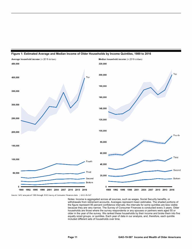
income of households in the bottom 20 percent was about $14,000, which is about 55 percent higher.11 We found similar results when we analyzed changes in median income.
11All amounts in this report are presented in 2016 dollars. As another example, households in the middle quintile in 2016 had estimated average income of about $53,000. In addition, we estimated that, in 2016, all households in the bottom quintile had less than $22,000 in income; households in the second quintile had incomes between $22,000 and $40,000; households in the middle quintile had incomes between $40,000 and $69,000; households in the fourth (second-from-the-top) quintile had incomes between $69,000 and $123,000; and households in the top quintile had incomes over $123,000.
Page 11 GAO-19-587 Income and Wealth of Older Americans
Figure 1: Estimated Average and Median Income of Older Households by Income Quintiles, 1989 to 2016
Notes: Income is aggregated across all sources, such as wages, Social Security benefits, or withdrawals from retirement accounts. Averages represent mean estimates. The shaded portions of the figure represent 95 percent confidence intervals; the intervals for some quintiles are less visible because they are very narrow. The Survey of Consumer Finances is conducted every 3 years. Older households are those where the survey respondents or any spouses or partners were aged 55 or older in the year of the survey. We ranked these households by their income and broke them into five equally sized groups, or quintiles. Each year of data in our analysis, and, therefore, each quintile included different sets of households over time.
Page 12 GAO-19-587 Income and Wealth of Older Americans
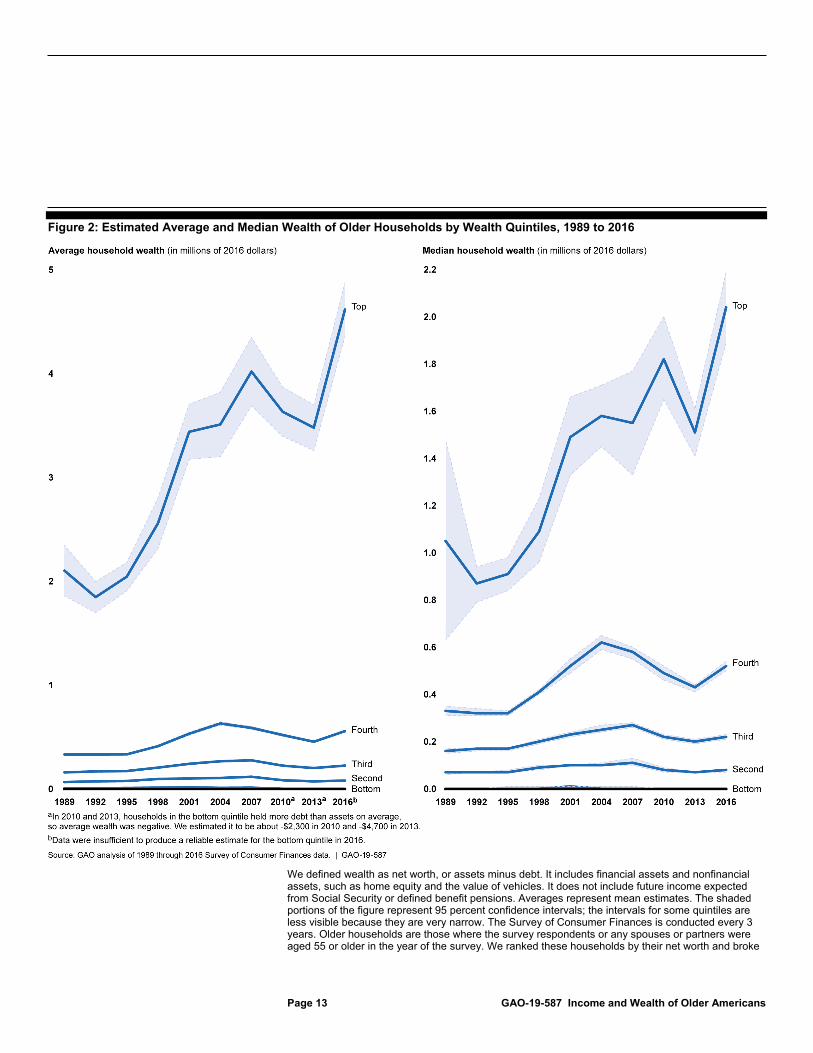
Our findings were similar when we analyzed changes in wealth (defined as net worth). Estimated average wealth of households in the top 20 percent was about $2.1 million in 1989. In 2016, estimated average wealth of households in the top 20 percent was about $4.6 million, which is more than twice as high. (See fig. 2.) In comparison, average wealth of households in the bottom 20 percent was similar over time from 1989 to 2013.12 In fact, in both 2010 and 2013, estimated average wealth of households that were in the bottom 20 percent in either of those years was negative, meaning that those households, on average, had more debt than assets.13 (See text box for discussion of how recessions during the time period of our analysis could affect retirement security.)
12There were insufficient data to produce a reliable estimate of average wealth for the bottom quintile in 2016. 13While the difference between estimates for 2016 and 1989 in the amount of average and median wealth held by the bottom 20 percent was relatively small compared to the differences for other quintiles, there were statistically significant differences among other particular years over the time period of our analysis. Also, there were insufficient data to produce a reliable estimate of average wealth for households in the bottom 20 percent in 2016. We estimate that average wealth for this group was about $4,500 in 1989. In 2010 and 2013, households in the bottom 20 percent, in either year, held more debt than assets, on average. As a result, estimated average wealth had negative values. In 2010, estimated average wealth was -$2,300. In 2013, estimated average wealth was -$4,700.
Page 13 GAO-19-587 Income and Wealth of Older Americans
Figure 2: Estimated Average and Median Wealth of Older Households by Wealth Quintiles, 1989 to 2016
We defined wealth as net worth, or assets minus debt. It includes financial assets and nonfinancial assets, such as home equity and the value of vehicles. It does not include future income expected from Social Security or defined benefit pensions. Averages represent mean estimates. The shaded portions of the figure represent 95 percent confidence intervals; the intervals for some quintiles are less visible because they are very narrow. The Survey of Consumer Finances is conducted every 3 years. Older households are those where the survey respondents or any spouses or partners were aged 55 or older in the year of the survey. We ranked these households by their net worth and broke
Page 14 GAO-19-587 Income and Wealth of Older Americans
them into five equally sized groups, or quintiles. Each year of data in our analysis, and, therefore, each quintile included different sets of households over time. When estimates were not available or had negative values, they were reset to zero for charting purposes.
Recessions and the Retirement Security of Older Americans Recessions can affect households’ resources in various ways. While there were three recessions during the period of our analysis (1990-1991, 2001, and 2007-2009), we were not able to disentangle the direct effects of the recessions on individual households’ income and wealth and, therefore, their retirement security. However, research on the 2007-2009 recession spotlights a few examples of how recessions could affect older Americans’ retirement security and suggests there could be varying effects across the income and wealth distributions. For example, others’ research shows the 2007-2009 recession affected high-income earners disproportionately because they were more likely to hold riskier assets, such as stocks, and the recession was rooted in a financial crisis. However, even though the effects on wealth may have been disproportionate, the effects may have been felt across the distribution. For example, many families saw their wealth decline during this recession. The decline in housing values surrounding this recession affected many low- and moderate-wealth families as home equity was a large share of their total assets. To the extent that home equity is an important source of wealth for older Americans, declines in housing values could create financial difficulties. In addition, our prior work has demonstrated that when older workers lose their job, like in a recession, it takes them longer to find another job and this could affect retirement security. In 2012, we found long-term unemployment can put older workers at risk of deferring needed medical care, losing their homes, and accumulating debt. Also, long-term unemployment can substantially diminish an older worker’s future retirement income in a couple of ways. First, it can force a worker to stop working and stop saving for retirement earlier than the worker had planned. Second, long-term unemployment can lead individuals to draw down their retirement accounts to cover living expenses while they are unemployed, which was a common life experience described by focus group participants with whom we spoke.
Source: GAO summary of Michael T. Owyang and Hannah G. Shell, “Taking Stock: Income Inequality and the Stock Market,” Economic Synopses, vol. 2016, no. 7 (St. Louis: Federal Reserve Bank of St. Louis, 2016); Sarah Bloom Raskin, “Downturns and Recoveries: What the Economies in Los Angeles and the United States Tell Us” (remarks at the Luncheon for Los Angeles Business and Community Leaders, Los Angeles Branch of the Federal Reserve Bank of San Francisco, April 12, 2012); GAO, Unemployed Older Workers: Many Experience Challenges Regaining Employment and Face Reduced Retirement Security, GAO-12-445 (Washington, D.C.: April 25, 2012); and documents from the Business Cycle Dating Committee of the National Bureau of Economic Research. | GAO-19-587
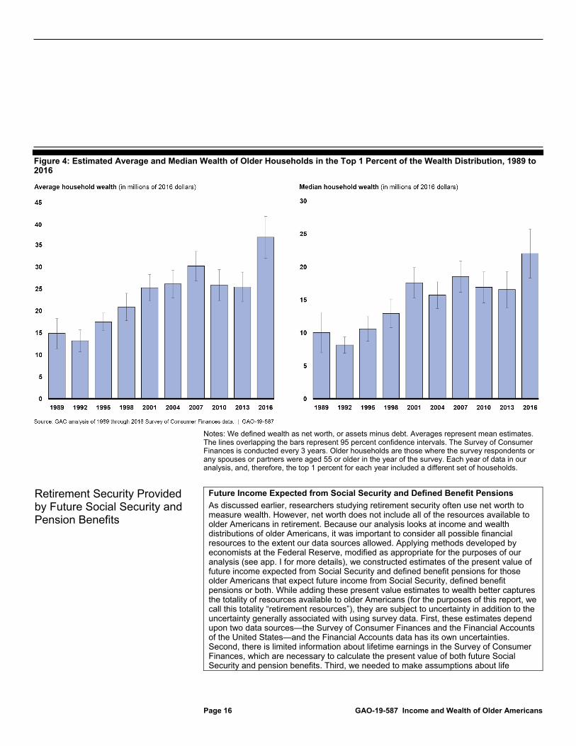
Within the top quintile, a disproportionate share of income and wealth is held by the top 1 percent compared to the next 19 percent.14 (See figs. 3 and 4 for average income and wealth of households in the top 1 percent.) For example, we found households in the top 1 percent in 1989 had estimated average wealth that was about $13 million more than estimated average wealth for households in the next 19 percent (about 10 times as much estimated average wealth). By 2016, households in the top 1 14For more details on the demographic and financial characteristics associated with the top 1 percent of households, see appendix II. This appendix also contains information on these characteristics for the next 19 percent, the top quintile, the bottom 80 percent, and the bottom quintile.
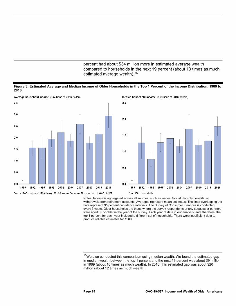
Page 15 GAO-19-587 Income and Wealth of Older Americans
percent had about $34 million more in estimated average wealth compared to households in the next 19 percent (about 13 times as much estimated average wealth).15
Figure 3: Estimated Average and Median Income of Older Households in the Top 1 Percent of the Income Distribution, 1989 to 2016
Notes: Income is aggregated across all sources, such as wages, Social Security benefits, or withdrawals from retirement accounts. Averages represent mean estimates. The lines overlapping the bars represent 95 percent confidence intervals. The Survey of Consumer Finances is conducted every 3 years. Older households are those where the survey respondents or any spouses or partners were aged 55 or older in the year of the survey. Each year of data in our analysis, and, therefore, the top 1 percent for each year included a different set of households. There were insufficient data to produce reliable estimates for 1989.
15We also conducted this comparison using median wealth. We found the estimated gap in median wealth between the top 1 percent and the next 19 percent was about $9 million in 1989 (about 10 times as much wealth). In 2016, this estimated gap was about $20 million (about 12 times as much wealth).
Page 16 GAO-19-587 Income and Wealth of Older Americans
Figure 4: Estimated Average and Median Wealth of Older Households in the Top 1 Percent of the Wealth Distribution, 1989 to 2016
Notes: We defined wealth as net worth, or assets minus debt. Averages represent mean estimates. The lines overlapping the bars represent 95 percent confidence intervals. The Survey of Consumer Finances is conducted every 3 years. Older households are those where the survey respondents or any spouses or partners were aged 55 or older in the year of the survey. Each year of data in our analysis, and, therefore, the top 1 percent for each year included a different set of households.
Future Income Expected from Social Security and Defined Benefit Pensions As discussed earlier, researchers studying retirement security often use net worth to measure wealth. However, net worth does not include all of the resources available to older Americans in retirement. Because our analysis looks at income and wealth distributions of older Americans, it was important to consider all possible financial resources to the extent our data sources allowed. Applying methods developed by economists at the Federal Reserve, modified as appropriate for the purposes of our analysis (see app. I for more details), we constructed estimates of the present value of future income expected from Social Security and defined benefit pensions for those older Americans that expect future income from Social Security, defined benefit pensions or both. While adding these present value estimates to wealth better captures the totality of resources available to older Americans (for the purposes of this report, we call this totality “retirement resources”), they are subject to uncertainty in addition to the uncertainty generally associated with using survey data. First, these estimates depend upon two data sources—the Survey of Consumer Finances and the Financial Accounts of the United States—and the Financial Accounts data has its own uncertainties. Second, there is limited information about lifetime earnings in the Survey of Consumer Finances, which are necessary to calculate the present value of both future Social Security and pension benefits. Third, we needed to make assumptions about life
Retirement Security Provided by Future Social Security and Pension Benefits
Page 17 GAO-19-587 Income and Wealth of Older Americans
expectancy, real discount rates, and retirement ages, which are unlikely to hold for all households, and which are themselves sources of uncertainty. As a result, we conducted some sensitivity analyses, particularly with respect to discount rates and retirement ages. For reporting purposes, we chose age 62 as the retirement age for the present value calculation of Social Security benefits, similar to the methods applied by economists at the Federal Reserve. It is possible that setting the retirement age at 62 may overstate the present value of future Social Security benefits, depending on various factors including interest rates and mortality. We considered using alternative retirement ages and do not believe that choosing a different retirement age for those not yet retired would substantively change our findings.
Source: GAO analysis. | GAO-19-587
Social Security is the foundation of retirement security in the United States, and along with income from traditional DB pensions, can be particularly important for older households with lower wealth. As discussed in the text box above, some older Americans will expect future income from Social Security, DB pensions or both.16 We analyzed the present value of these sources for two subsets of older Americans: 1) those who expect future income from Social Security but not DB pensions, and 2) those who expect future income from both Social Security and DB pensions.17
16We estimated the percentage of households in each quintile that expected no future income from Social Security or DB pensions, future income from Social Security only, future income from DB pensions only, or future income from both sources. For example, in 2016, about 73 percent of households in the bottom quintile expected future income from Social Security only while 23 percent expected future income from Social Security and DB pensions. The remaining 4 percent expected future income from DB pensions only or no future income from Social Security or DB pensions. For the top quintile, 54 percent of households expected future income from Social Security only while 46 percent expected future income from Social Security and DB pensions. 17We say “estimated present value” because our estimates are based on assumptions about the future, as well as the time value of money, and may not be the actual amount that will be received. For example, as previously discussed, unless changes are made, the Social Security Old Age and Survivors Insurance Trust Fund faces projected depletion in 2034, at which point this Trust Fund is estimated to be sufficient to pay only 77 percent of scheduled benefits. Further, our estimates rely on assumptions about life expectancy, discount rates, and retirement ages, which are unlikely to hold for all households. As a result, we conducted some sensitivity analyses, particularly with respect to discount rates and retirement ages. To produce these estimates, we applied methods developed by economists at the Federal Reserve, with modifications appropriate for the purposes of our analysis. The Federal Reserve economists continue to refine their methodology and we relied on recently available papers as a starting point for our analysis. For more on the Federal Reserve economists’ method, see Devlin-Foltz, Henriques, and Sabelhaus, “Is the U.S. Retirement System Contributing to Rising Wealth Inequality?” (2016). For more information on these methods, including sensitivity analyses we performed to better understand how certain assumptions affected our results, see appendix I.
Page 18 GAO-19-587 Income and Wealth of Older Americans
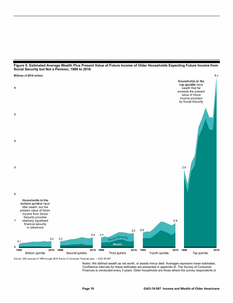
On average, households with lower wealth,18 and that expect future income from Social Security but not DB pensions, may receive a significant income stream from future Social Security benefits, according to our analysis of SCF data (see fig. 5). The bottom 20 percent have little in wealth, on average, but the estimated present value of future Social Security benefits provides them relatively significant financial security in retirement. On the other hand, for the top two quintiles, wealth was the most important retirement resource, as households in the top quintile have wealth that, on average, far exceeds the estimated present value of benefits provided by any future Social Security or pension benefits.
18We defined wealth as net worth (assets minus debt).
Page 19 GAO-19-587 Income and Wealth of Older Americans
Figure 5: Estimated Average Wealth Plus Present Value of Future Income of Older Households Expecting Future Income from Social Security but Not a Pension, 1989 to 2016
Notes: We defined wealth as net worth, or assets minus debt. Averages represent mean estimates. Confidence intervals for these estimates are presented in appendix III. The Survey of Consumer Finances is conducted every 3 years. Older households are those where the survey respondents or
Page 20 GAO-19-587 Income and Wealth of Older Americans
any spouses or partners were aged 55 or older in the year of the survey. We ranked these households by their wealth (net worth) and broke them into five equally sized groups, or quintiles. Each year of data in our analysis, and, therefore, each quintile included different sets of households over time. This figure includes only those households in each quintile that expected to receive future income from Social Security but not defined benefit pensions. For example, in 2016, 73 percent of households in the bottom quintile expected to receive future income from Social Security but not defined benefit pensions. Corresponding percentages for the second through fifth (or top) quintiles were 61, 50, 46, and 54 percent. Average wealth for the bottom quintile was negative (debt was greater than assets) in 2010 and 2013, with values of about -$4,000 and -$7,000, respectively. We estimated that, for the bottom quintile, retirement resources (the present value of future income expected from Social Security plus net worth) totaled about $219,000 in 2010 and $197,000 in 2013. There were insufficient data to produce an estimate of wealth for the bottom quintile in 2016. When estimates were not available or had negative values, they were reset to zero for charting purposes.
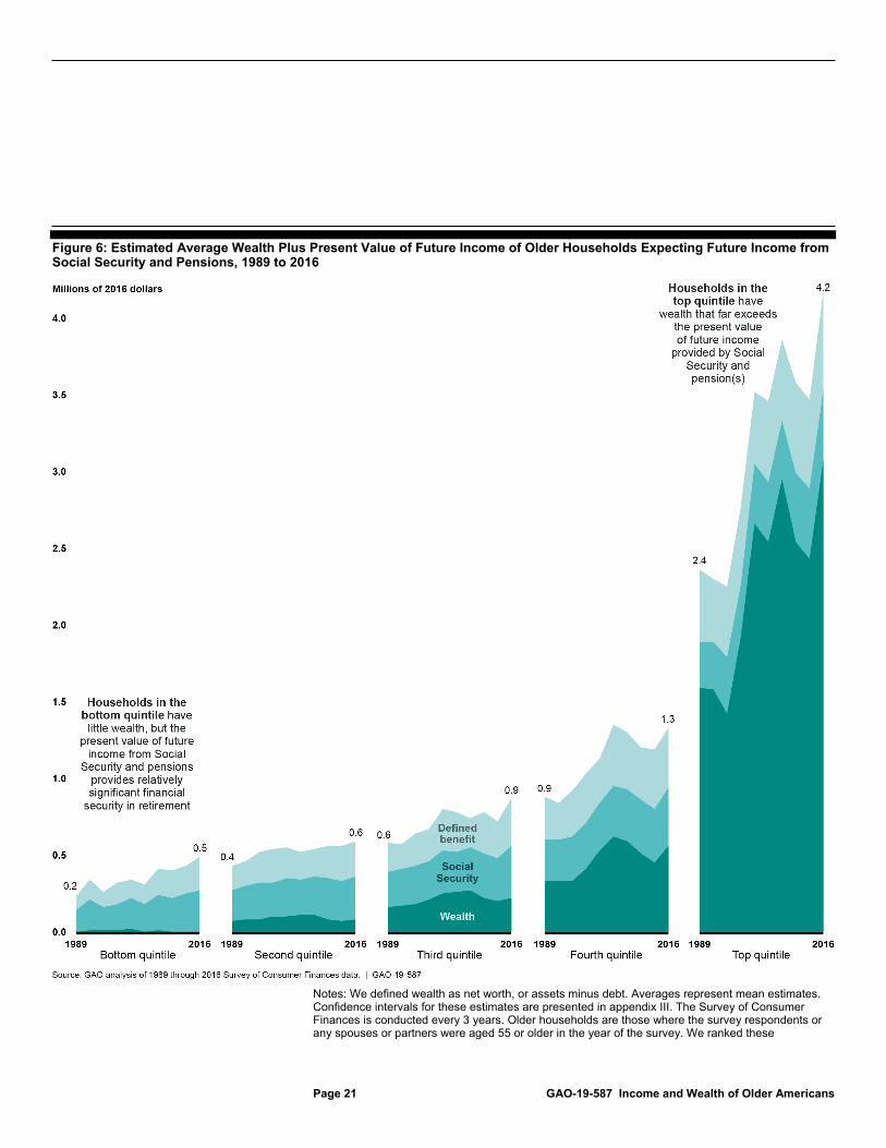
We found similar results for households with lower wealth and that expect future income from Social Security and DB pensions. While the lower quintiles may have little in wealth, on average, they may expect to receive a significant income stream from future Social Security and DB pension benefits (see fig. 6). Wealth was the most important financial retirement resource for the top two quintiles, on average.
Page 21 GAO-19-587 Income and Wealth of Older Americans
Figure 6: Estimated Average Wealth Plus Present Value of Future Income of Older Households Expecting Future Income from Social Security and Pensions, 1989 to 2016
Notes: We defined wealth as net worth, or assets minus debt. Averages represent mean estimates. Confidence intervals for these estimates are presented in appendix III. The Survey of Consumer Finances is conducted every 3 years. Older households are those where the survey respondents or any spouses or partners were aged 55 or older in the year of the survey. We ranked these
Page 22 GAO-19-587 Income and Wealth of Older Americans
households by their wealth (net worth) and broke them into five equally sized groups, or quintiles. Each year of data in our analysis, and, therefore, each quintile included different sets of households over time. This figure includes only those households in each quintile that expected to receive future income from Social Security and defined benefit pensions. For example, in 2016, 23 percent of households in the bottom quintile expected to receive future income from Social Security and defined benefit pensions. Corresponding percentages for the second through fifth (or top) quintiles were 38, 49, 54, and 46 percent. There were insufficient data to produce an estimate of wealth for the bottom quintile in 1989, 2004, 2010, 2013, and 2016. When estimates were not available, they were reset to zero for charting purposes.
While disparities remain, the present value of future income expected from Social Security and DB pensions mitigate these disparities to some extent for those households that expected such income, as illustrated by the examples below.
• Estimates for all older households in 2016 that expect future income from Social Security but not DB pensions: Households in the top quintile had, on average, about $6.1 million in assets, about 272 times as much as the bottom quintile, which had estimated assets of, on average, about $22,000.19 When looking at a broader definition of retirement resources (assets plus the present value of future income from Social Security), we estimated that the top quintile had, on average, $6.6 million in these resources, about 27 times as much as the bottom quintile, which had, on average, about $241,000.
• Estimates for all older households in 2016 that expect future income from Social Security and DB pensions: Households in the top quintile had, on average, about $3.2 million in assets, about 61 times as much in assets as the bottom quintile, which had estimated assets of, on average, about $52,000.20 When looking at a broader definition of retirement resources (assets plus the present value of future income from Social Security and DB pensions), we estimated that the top quintile had, on average, about $4.3 million in these resources, about
19We use assets in this example because there were insufficient data to estimate net worth for the bottom quintile of the wealth distribution in 2016. We estimated average net worth of $5.9 million for households in the top quintile that future income expected from Social Security but not DB pensions. We estimated that, for these households, the combined total of wealth (net worth) plus the present value of future income expected from Social Security was $6.4 million, on average. 20We use assets in this example because there were insufficient data to estimate net worth for the bottom quintile of the wealth distribution in 2016. We estimated average net worth of $3.1 million for households in the top quintile that expected future income from Social Security and DB pensions. We estimated that, for these households, the combined total of wealth (net worth) plus the present value of expected future income from Social Security and DB pensions was $4.2 million, on average.
Page 23 GAO-19-587 Income and Wealth of Older Americans
8 times as much as the bottom quintile, which had, on average, about $535,000.
Recent research has theorized that benefits expected from Social Security “[go] a long way” to explaining why having little in DC accounts and future income expected from pensions does not necessarily translate into dramatic changes to living standards as people retire.21 In particular, the progressivity of Social Security, meaning Social Security benefits replace a higher percentage of pre-retirement earnings for lower-earning households, could be helpful for these households, especially in the absence of other resources, such as retirement accounts.22
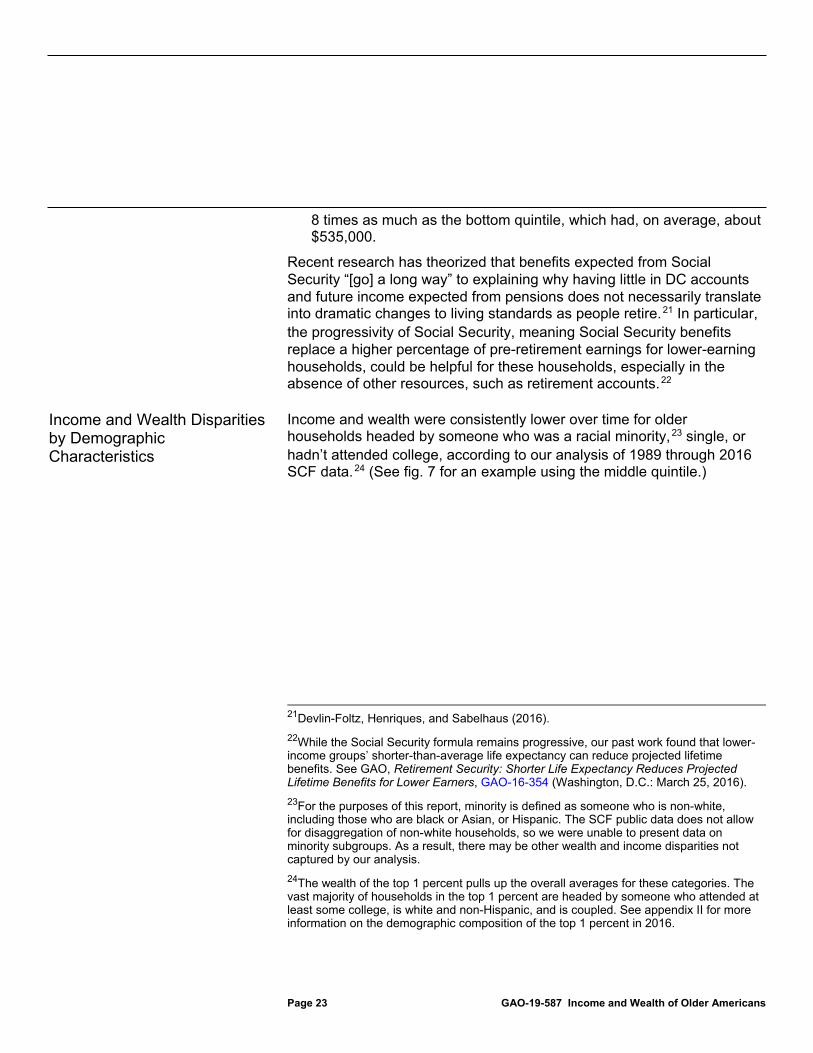
Income and wealth were consistently lower over time for older households headed by someone who was a racial minority,23 single, or hadn’t attended college, according to our analysis of 1989 through 2016 SCF data.24 (See fig. 7 for an example using the middle quintile.)
21Devlin-Foltz, Henriques, and Sabelhaus (2016). 22While the Social Security formula remains progressive, our past work found that lower-income groups’ shorter-than-average life expectancy can reduce projected lifetime benefits. See GAO, Retirement Security: Shorter Life Expectancy Reduces Projected Lifetime Benefits for Lower Earners, GAO-16-354 (Washington, D.C.: March 25, 2016). 23For the purposes of this report, minority is defined as someone who is non-white, including those who are black or Asian, or Hispanic. The SCF public data does not allow for disaggregation of non-white households, so we were unable to present data on minority subgroups. As a result, there may be other wealth and income disparities not captured by our analysis. 24The wealth of the top 1 percent pulls up the overall averages for these categories. The vast majority of households in the top 1 percent are headed by someone who attended at least some college, is white and non-Hispanic, and is coupled. See appendix II for more information on the demographic composition of the top 1 percent in 2016.
Income and Wealth Disparities by Demographic Characteristics
Page 24 GAO-19-587 Income and Wealth of Older Americans
Figure 7: Estimated Wealth of Older Households in the Middle Quintile of the Wealth Distribution by Race and Ethnicity, Education, and Marital Status, 1989 to 2016
Notes: We defined wealth as net worth, or assets minus debt. Averages represent mean estimates. The lines overlapping the bars represent 95 percent confidence intervals. The Survey of Consumer Finances is conducted every 3 years. Older households are those where the survey respondents or any spouses or partners were aged 55 or older in the year of the survey. We defined minority as someone who is non-white, including those who are black or Asian, or Hispanic. We ranked these
Page 25 GAO-19-587 Income and Wealth of Older Americans
households by their net worth and broke them into five equally sized groups, or quintiles. Each year of data in our analysis, and, therefore, each quintile included different sets of households over time.
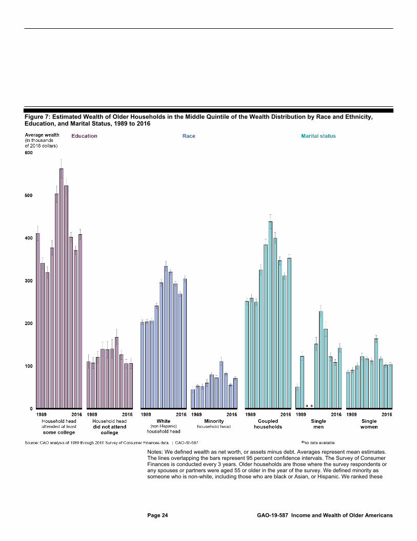
We found these disparities existed across all quintiles and all years (see fig. 8 for another example, this time using the top quintile).25 Generally, the largest disparities from 1989 to 2016 were between 1) households in which the head had not attended college and households in which they had and 2) coupled households and single women. These results are consistent with our prior work, which found that women age 65 and older had less retirement income, on average, and live in higher rates of poverty than men in that age group.26 Disparities were also sizeable for households headed by someone who was white and non-Hispanic compared to those headed by a minority.27
25Household heads who attended college did not necessarily earn a degree. 26GAO, Retirement Security: Women Still Face Challenges, GAO-12-699 (Washington, D.C.: July 19, 2012). GAO has forthcoming work with more analysis of women’s retirement income security. 27Preliminary research from researchers at the Center for Retirement Research at Boston College estimates that the value of expected future income from Social Security has a mitigating effect on racial and ethnic disparities in wealth. See Hou, Wenliang and Geoffrey T. Sanzenbacher, “Measuring Racial/Ethnic Inequality in Retirement Wealth” (paper presented at the 21st Annual Social Security Administration Research Consortium Meeting, Washington, D.C., Aug. 2019).
Page 26 GAO-19-587 Income and Wealth of Older Americans
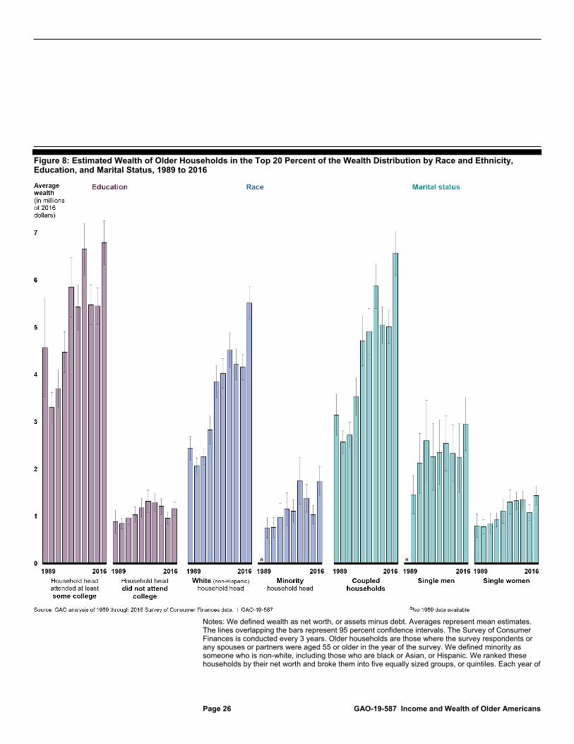
Figure 8: Estimated Wealth of Older Households in the Top 20 Percent of the Wealth Distribution by Race and Ethnicity, Education, and Marital Status, 1989 to 2016
Notes: We defined wealth as net worth, or assets minus debt. Averages represent mean estimates. The lines overlapping the bars represent 95 percent confidence intervals. The Survey of Consumer Finances is conducted every 3 years. Older households are those where the survey respondents or any spouses or partners were aged 55 or older in the year of the survey. We defined minority as someone who is non-white, including those who are black or Asian, or Hispanic. We ranked these households by their net worth and broke them into five equally sized groups, or quintiles. Each year of
Page 27 GAO-19-587 Income and Wealth of Older Americans
data in our analysis, and, therefore, each quintile included different sets of households over time. The wealth of the top 1 percent pulls up the overall averages for these categories. The vast majority of households in the top one percent are headed by someone who attended at least some college, are white and non-Hispanic, and are coupled.
There are multiple reasons why households headed by someone with at least some college education may have more wealth in retirement. Most notably, those with more education may have access to higher-paying jobs and be able to save more. Our review of the literature identified several other theories to explain this association. These include (1) education increases awareness about the need to save, (2) highly-educated individuals may have more financial education and achieve higher rates of return on savings, (3) those with more education may be willing to work longer, and (4) highly-educated individuals may have wealthier parents and thus may have received larger bequests.28 Our prior work has explored how recent trends in marital patterns and saving for retirement, among other factors, can negatively affect retirement security for minorities, women, or those who are single.29
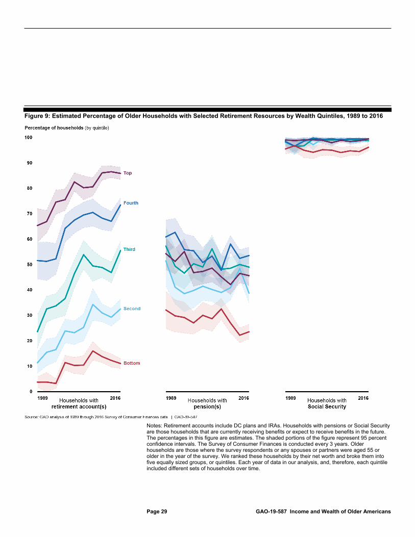
The percentage of households with retirement accounts was higher across all wealth quintiles in 2016 compared to 1989, and it was disproportionately higher for the top quintile, according to our analysis of SCF data. In 1989, the percentage of households with retirement accounts—amounts in DC plans and IRAs—ranged from 4 percent of the bottom quintile to 65 percent of the top quintile (see fig. 9). By 2016, 11 percent of households in the bottom quintile had retirement accounts compared to 86 percent of households in the top quintile. These increases reflect the transition to more employers offering DC plans, among other factors.30 Further, the percentage of households in the bottom quintile with retirement accounts had not returned to its pre-
28James Poterba, Steven Venti, and David A. Wise, “Longitudinal Determinants of End-of-Life Wealth Inequality,” Journal of Public Economics, vol. 162 (2018); Brookings Economic Studies Program, Later Retirement, Inequality in Old Age, and the Growing Gap in Longevity between Rich and Poor (Washington, D.C.: Brookings Institution, 2016). 29GAO-18-111SP; GAO, Retirement Security: Low Defined Contribution Savings May Pose Challenges, GAO-16-408 (Washington, D.C.: May 5, 2016); and Retirement Security: Trends in Marriage and Work Patterns May Increase Economic Vulnerability for Some Retirees, GAO-14-33 (Washington, D.C.: January 15, 2014). 30For more on the transition to more employers offering DC plans, and the rise in assets in DC plans and IRAs, see GAO-18-111SP.
Percentage of Older Households with Retirement Accounts Has Increased Since 1989, Although Non-Retirement Assets Remain Important
Page 28 GAO-19-587 Income and Wealth of Older Americans
recession rate.31 As discussed earlier, households with less wealth may be more reliant on income from Social Security and DB plans.
31In 2007, 16 percent of households in the bottom quintile had retirement accounts. This result is statistically significant at the 95 percent confidence level. The difference in the percentage of households with retirement accounts from 2007 to 2016 was not statistically significant for the second through fourth quintiles, although it was statistically significant for the top quintile.
Page 29 GAO-19-587 Income and Wealth of Older Americans
Figure 9: Estimated Percentage of Older Households with Selected Retirement Resources by Wealth Quintiles, 1989 to 2016
Notes: Retirement accounts include DC plans and IRAs. Households with pensions or Social Security are those households that are currently receiving benefits or expect to receive benefits in the future. The percentages in this figure are estimates. The shaded portions of the figure represent 95 percent confidence intervals. The Survey of Consumer Finances is conducted every 3 years. Older households are those where the survey respondents or any spouses or partners were aged 55 or older in the year of the survey. We ranked these households by their net worth and broke them into five equally sized groups, or quintiles. Each year of data in our analysis, and, therefore, each quintile included different sets of households over time.
Page 30 GAO-19-587 Income and Wealth of Older Americans
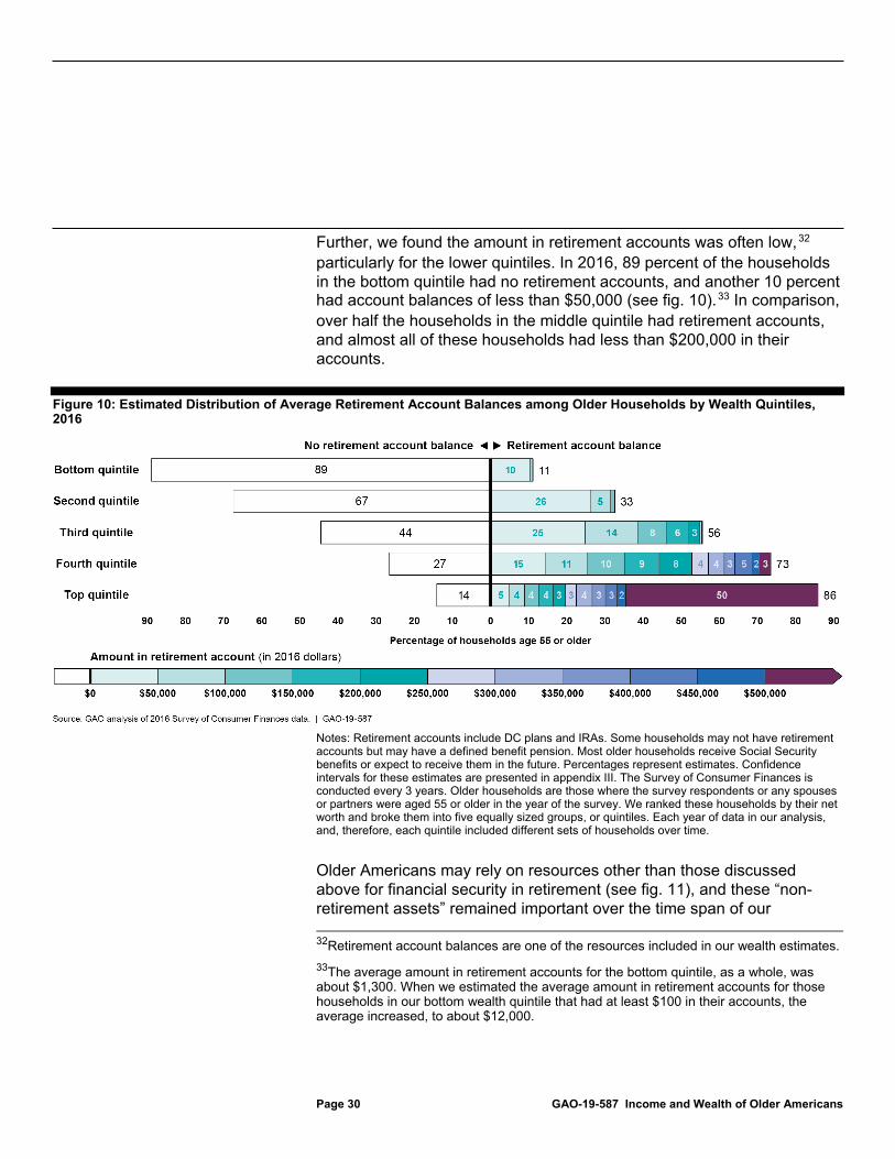
Further, we found the amount in retirement accounts was often low,32 particularly for the lower quintiles. In 2016, 89 percent of the households in the bottom quintile had no retirement accounts, and another 10 percent had account balances of less than $50,000 (see fig. 10).33 In comparison, over half the households in the middle quintile had retirement accounts, and almost all of these households had less than $200,000 in their accounts.
Figure 10: Estimated Distribution of Average Retirement Account Balances among Older Households by Wealth Quintiles, 2016
Notes: Retirement accounts include DC plans and IRAs. Some households may not have retirement accounts but may have a defined benefit pension. Most older households receive Social Security benefits or expect to receive them in the future. Percentages represent estimates. Confidence intervals for these estimates are presented in appendix III. The Survey of Consumer Finances is conducted every 3 years. Older households are those where the survey respondents or any spouses or partners were aged 55 or older in the year of the survey. We ranked these households by their net worth and broke them into five equally sized groups, or quintiles. Each year of data in our analysis, and, therefore, each quintile included different sets of households over time.
Older Americans may rely on resources other than those discussed above for financial security in retirement (see fig. 11), and these “non-retirement assets” remained important over the time span of our 32Retirement account balances are one of the resources included in our wealth estimates. 33The average amount in retirement accounts for the bottom quintile, as a whole, was about $1,300. When we estimated the average amount in retirement accounts for those households in our bottom wealth quintile that had at least $100 in their accounts, the average increased, to about $12,000.
Page 31 GAO-19-587 Income and Wealth of Older Americans
analysis,34 regardless of their value relative to retirement account balances or the present value of future income from Social Security or DB pensions.
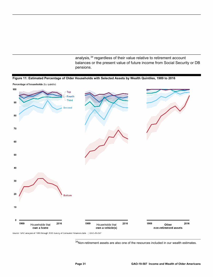
Figure 11: Estimated Percentage of Older Households with Selected Assets by Wealth Quintiles, 1989 to 2016
34Non-retirement assets are also one of the resources included in our wealth estimates.
Page 32 GAO-19-587 Income and Wealth of Older Americans
Notes: The percentages in this figure are estimates. The shaded portions of the figure represent 95 percent confidence intervals. The Survey of Consumer Finances is conducted every 3 years. Older households are those where the survey respondents or any spouses or partners were aged 55 or older in the year of the survey. We ranked these households by their net worth and broke them into five equally sized groups, or quintiles. Each year of data in our analysis, and, therefore, each quintile included different sets of households over time. For the bottom quintile, the higher percentage of households with all other non-retirement assets in 2016 relative to other years is partly due to the Survey of Consumer Finances including pre-paid debit cards in the survey for the first time in 2016. See Board of Governors of the Federal Reserve System, “Changes in U.S. Family Finances from 2013 to 2016: Evidence from the Survey of Consumer Finances,” Federal Reserve Bulletin, vol. 103, no. 3 (Washington, D.C.: September 2017).
• Home equity. We estimated that over 80 percent of households in each of the top four quintiles of the wealth distribution owned a home in each year of our analysis. However, the home ownership rate for households in the bottom quintile in each year of our analysis was consistently much lower than for the other quintiles–ranging between 18 and 32 percent. Further, the home ownership rate for households in the bottom 20 percent in 2016 (19 percent) was significantly lower than the home ownership rate for households in the bottom 20 percent in 2007 (28 percent), the starting year for the most recent recession.35 In 2016, the estimated average amount of home equity of households in the bottom quintile was about $2,000, and $50,000 for the second-from-the-bottom quintile, compared to about $118,000 for the middle quintile, about $208,000 for the fourth (or second-from-the-top) quintile, and about $559,000 for the top quintile. According to researchers, most households appear to treat a house as a source of reserve wealth that can be tapped in the event of a substantial expense, further pointing to the importance of home ownership for many older Americans.36
• Vehicles. A majority of households in each quintile of the wealth distribution owned a vehicle across all years in our analysis, although the bottom quintile had ownership rates that were disproportionately lower. However, despite this, we estimated that vehicles provided higher value, on average, relative to other non-retirement assets for households in the bottom quintile from 2010 onward. For example, in 2016, the estimated average value of vehicles among households in the bottom quintile was about $7,000 in 2016, compared to estimated
35Differences in the percentage of households that owned a home from 2007 to 2016 were statistically significant at the 95 percent confidence level for the bottom two quintiles. These differences were not statistically significant for the top three quintiles. 36Poterba et al., “The Composition and Drawdown of Wealth in Retirement,” Journal of Economic Perspectives, vol. 25, no. 4 (2011).
Page 33 GAO-19-587 Income and Wealth of Older Americans
average values of less than $2,000 in home equity and about $3,000 in all other non-retirement assets.
• All-other non-retirement assets. For the top quintile of households, the average value of these “other assets”—which included stocks, bonds, and other savings outside of retirement accounts,37 among other things—was more than average home equity or the average value of vehicles over the period of our analysis. Estimated average wealth in this other assets category was about $3.3 million in 2016 for the top quintile.38
Individual income sources and debt were also important factors in older households’ financial security. Researchers have examined the importance of income sources for households and found Social Security is more important for households with lower incomes, while older households with the most income tend to have a diverse range of income sources, such as earnings from financial assets and income from DB plans.39 We found that debt could have a substantial effect on households’ financial security, particularly for the bottom 20 percent. For example, in 2010 and 2013, average net worth for this group was negative because debt was greater than assets.
37Other savings outside retirement accounts includes assets such as savings accounts, checking accounts, money market accounts and, as of the 2016 survey, prepaid cards. 38We also estimated the average value of home equity, vehicles, and all-other non-retirement assets for households in each quintile that had at least $100 in the asset. The averages were similar to the estimated averages included in these bullet points. 39Anqi Chen, Alicia H. Munnell, and Geoffrey T. Sanzenbacher. “How Much Income Do Retirees Actually Have? Evaluating the Evidence from Five National Datasets,” Center for Retirement Research Working Paper, vol. 2018-14 (2018); and Adam Bee and Joshua Mitchell, “Do Older Americans Have More Income Than We Think?” SESHD Working Paper, vol. 2017-39 (2017).

Page 34 GAO-19-587 Income and Wealth of Older Americans
A substantial number of older Americans born from 1931 through 1941 lived into at least their 70s or early 80s, according to our analysis of data on a cohort of people born in these years.40 (See text box and app. I for more on how we analyzed Health and Retirement Study (HRS) data on this cohort.) However, this same cohort faced disparities in longevity.41 Further, our analysis, as well as that of other researchers, found income and wealth each have strong associations with longevity, as do certain demographic characteristics, such as gender and race.42 However, even among those with multiple factors associated with a shorter life, such as having lower mid-career earnings and not having attended college, a significant proportion from our cohort were alive in 2014, when they were in their 70s or early 80s. Taken all together, individuals may live a long time, even individuals with factors associated with lower longevity, such as low income or education. Those who live a long time and have little or nothing in DC account balances or pension benefits may have to rely primarily on Social Security or safety net programs.
Analyzing Income, Wealth and Longevity We examined the association of income and wealth with longevity in a nationally representative sample of Americans born from 1931 through 1941. Throughout this analysis, our references to “older Americans” and “households” apply to that specific subset of older Americans born from 1931 through 1941 and their households. The Health and Retirement Study (HRS) began in 1992 and first surveyed these individuals when they were 51 to 61 years old. The same individuals have been re-interviewed every 2 years since, provided they continued to participate in the survey, and the most recent complete data is from 2014, when those who were still alive were 73 to 83 years old. We were able to measure deaths over a period of 22 years (1992 through 2014). Every 2 years, the HRS attempted to measure whether the original respondents were still alive, but these longevity data were incomplete because some of the original respondents declined to participate in later waves of the survey. Once these respondents left the survey, their actual longevity could not be followed. Therefore, we used survival analysis to estimate the proportion of individuals in the1992 sample alive in 2014. Survival analysis accounts for survey respondents with complete
40Our analysis only covers the years up to when members of this cohort reached ages ranging from 73 to 83. Some of these individuals can be expected to live much longer. 41Since our data and analysis only covers the period when this cohort reached ages ranging from 73 to 83, it is only a partial longevity analysis in that it does not cover longevity beyond those ages. Therefore, our analysis of disparities in longevity within this cohort cannot address the extent to which such disparities might persist beyond these age ranges. While we could use the more technical term “survivorship” to refer to disparities over our observation period, we use the more familiar term “longevity” in this report. 42For details on our review of other researchers’ work and interviews with several of these researchers, see appendix I.
A Substantial Number of Older Americans Are Living Into Their Seventies or Early Eighties, Which May Have Implications for Retirement Security
Page 35 GAO-19-587 Income and Wealth of Older Americans
or incomplete longevity data and allowed us to estimate the chance of death by any given time in the observation period. Most importantly, our analysis assumed actual longevity from 1992 to 2014 of the individuals in our analysis did not have a systematic relationship with whether the original HRS respondents continued to participate in the study except that leaving the study implied a later death. We believe this assumption to be reasonable for the purpose of our analysis for two reasons. First, a small percentage (8 percent) of the original respondents dropped out of the survey, so that the impact of any longevity differences among the population who dropped out would likely have been small. Second, while some baseline characteristics of respondents do appear correlated with non-response over time, the population that dropped out of the study does not appear to vary significantly from those completing each wave, except for race and ethnicity. We conducted this analysis, at the individual level, for HRS respondents in 1992, and any spouses or partners also born in 1931 through 1941. Additional details and caveats to this analysis are available in appendix I. We broke the sample into quintiles based on their income or wealth. To determine an individual’s place in the income distribution, we measured mid-career household earnings using administrative records from the Social Security Administration that are linked to the HRS data. Specifically, we defined mid-career household earnings based on average annual earnings reported to the Social Security Administration for years when the survey respondent we identified as the household head was ages 41 to 50 as well as the earnings of their spouse or partner during those years if the respondent was part of a couple in 1992. This measure of earnings provides a relatively stable indicator of the household’s labor market experience, compared to using a single year of earnings, which could be unusually high or low. For wealth, we used the household’s initial net worth in 1992, including any balances in defined contribution accounts or individual retirement accounts, but excluding second homes, which HRS did not consistently capture in all years. In both instances, the sample was broken into quintiles. For additional details on our methodology, see appendix I.
Source: GAO analysis of 1992 through 2014 HRS data. | GAO-19-587
Overall, an estimated 63 percent of the individuals in our sample were alive in 2014 (ages 73 to 83), and greater levels of income and wealth were associated with greater longevity in our analysis of HRS data.43 For income, an estimated 52 percent of individuals from households in the bottom quintile of the mid-career earnings distribution were alive in 2014, compared to an estimated 74 percent of individuals from households in the top quintile. (See fig. 12.) The percentages by wealth quintile were similar.44 Other researchers have similarly found that greater levels of income and wealth are associated with greater longevity. For example, a researcher at the Social Security Administration has established that men
43We measured income using our mid-career earnings measure. We measured wealth (defined as net worth) as of 1992, the year the cohort was first interviewed for the HRS. 44See appendix IV for results from this analysis.
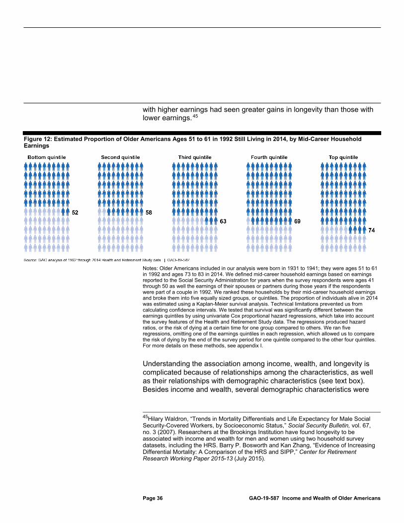
Page 36 GAO-19-587 Income and Wealth of Older Americans
with higher earnings had seen greater gains in longevity than those with lower earnings.45
Figure 12: Estimated Proportion of Older Americans Ages 51 to 61 in 1992 Still Living in 2014, by Mid-Career Household Earnings
Notes: Older Americans included in our analysis were born in 1931 to 1941; they were ages 51 to 61 in 1992 and ages 73 to 83 in 2014. We defined mid-career household earnings based on earnings reported to the Social Security Administration for years when the survey respondents were ages 41 through 50 as well the earnings of their spouses or partners during those years if the respondents were part of a couple in 1992. We ranked these households by their mid-career household earnings and broke them into five equally sized groups, or quintiles. The proportion of individuals alive in 2014 was estimated using a Kaplan-Meier survival analysis. Technical limitations prevented us from calculating confidence intervals. We tested that survival was significantly different between the earnings quintiles by using univariate Cox proportional hazard regressions, which take into account the survey features of the Health and Retirement Study data. The regressions produced hazard ratios, or the risk of dying at a certain time for one group compared to others. We ran five regressions, omitting one of the earnings quintiles in each regression, which allowed us to compare the risk of dying by the end of the survey period for one quintile compared to the other four quintiles. For more details on these methods, see appendix I.
Understanding the association among income, wealth, and longevity is complicated because of relationships among the characteristics, as well as their relationships with demographic characteristics (see text box). Besides income and wealth, several demographic characteristics were
45Hilary Waldron, “Trends in Mortality Differentials and Life Expectancy for Male Social Security-Covered Workers, by Socioeconomic Status,” Social Security Bulletin, vol. 67, no. 3 (2007). Researchers at the Brookings Institution have found longevity to be associated with income and wealth for men and women using two household survey datasets, including the HRS. Barry P. Bosworth and Kan Zhang, “Evidence of Increasing Differential Mortality: A Comparison of the HRS and SIPP,” Center for Retirement Research Working Paper 2015-13 (July 2015).
Page 37 GAO-19-587 Income and Wealth of Older Americans
also associated with longevity in our analysis of HRS data, and these relationships have also been noted in other researchers’ studies.46
• Women tended to live longer than men: Women had greater longevity through 2014, with an estimated 69 percent living to at least ages 73 to 83 compared to an estimated 58 percent of men.
• Non-Hispanic whites and Hispanics tended to live longer than blacks: For Hispanics, an estimated 68 percent lived to at least 2014, as did an estimated 65 percent of non-Hispanic whites, compared to an estimated 52 percent of non-Hispanic blacks.47
• More educated individuals tended to live longer than those with less education: An estimated 75 percent of college graduates lived to at least 2014, compared to an estimated 65 percent of those who graduated from high school and an estimated 50 percent of those with less than a high school diploma or GED.48
• Individuals who self-reported being in good health tended to live longer than those who reported being less healthy: Among those who self-reported being in excellent health in 1992, an estimated 78 percent lived to at least 2014, compared to an estimated 31 percent of those who reported being in poor health.
Income, Wealth, and Demographics Are Interrelated The relationships of income, wealth, and demographics with longevity are complex because of interactions among these characteristics themselves, which make it difficult to determine the direction or extent of causality. For example, there are many potential interactions among educational status, income, and wealth. Higher levels of education could provide access to better job opportunities, increasing income. Education could contribute to greater financial literacy and better financial decision making, increasing wealth. Having access to wealth could make it easier to attain additional education.
46See appendix IV for additional results across demographic categories. 47In the HRS, race and ethnicity are self-identified. For this analysis, sample sizes were sufficient to break out results by specific race and ethnicity categories. Our results regarding Hispanic longevity are similar to work by other researchers. See S. Jay Olshansky et al., “Differences in Life Expectancy Due to Race and Educational Differences Are Widening, and Many May Not Catch Up,” Health Affairs, vol. 31, no. 8 (2012) and John M. Ruiz, Patrick Steffen, and Timothy B. Smith, “Hispanic Mortality Paradox: A Systematic Review and Meta-Analysis of the Longitudinal Literature,” American Journal of Public Health, vol. 103, n0. 3 (February 2012). 48We relied on the head of household’s education level in 1992 for our measure of education.
Page 38 GAO-19-587 Income and Wealth of Older Americans
While income, wealth, and education all are associated with longevity, it is difficult to interpret their individual associations with longevity because of their possible interactions with each other.
Source: GAO analysis of studies included in our literature review. | GAO-19-587
We estimated that individuals whose households were in the top two quintiles (top 40 percent) of the mid-career earnings distribution were more likely than their counterparts in the bottom 60 percent to be alive in 2014 (ages 73 to 83) in an analysis controlling for race and ethnicity, gender, age, education level, and initial self-reported health status on entry into HRS in 1992.49 In a similar analysis, we found that individuals from households in the top quintile (top 20 percent) of wealth in 1992 were more likely to be alive than their counterparts in the bottom four quintiles. Our findings are consistent with the work of other researchers who also controlled for such factors. However, such observational studies are only able to demonstrate that a statistical association exists between two characteristics. For example, one study that found a strong association between income and life expectancy specifically notes that unmeasured factors likely affect the association.50 Similarly, we cannot determine from our analysis the extent to which income or wealth causes differences in longevity.
Even among individuals with characteristics associated with decreased longevity, a substantial proportion of older Americans lived at least into their 70s or early 80s, according to our analysis of 1992 to 2014 HRS data. For example, we constructed three scenarios to illustrate how longevity varies for those with different mid-career earnings and education.51 Among those in the “bottom” scenario–those individuals who had no college education and were from households in the bottom 20 percent of the earnings distribution–an estimated 50 percent were still alive in 2014 (see fig. 13).52 We estimated that the corresponding percentages for our “middle” scenario and “top” scenario were 65 percent 49See appendix IV for more detailed results. 50Raj Chetty et al., “The Association Between Income and Life Expectancy in the United States, 2001-2014,” JAMA, vol. 315, no. 16 (2016). 51These scenarios are three possible combinations of earnings and education out of many. They are intended to illustrate how income and demographic characteristics can interact and the potential effects they can have on longevity. In designing these scenarios, we considered the demographic factors discussed above as well as sample size constraints. 52We used the 1992 data to identify education levels.
Page 39 GAO-19-587 Income and Wealth of Older Americans
and 80 percent, respectively, of individuals still alive in 2014. Thus, even among those with education and earnings associated with lower longevity, a significant proportion, 50 percent, were still alive in 2014, and these individuals will need to provide for themselves through their remaining years.53 We also analyzed a subset of our bottom scenario that included those who had no college education and were from households in the bottom 20 percent of the earnings distribution and whose self-reported health status was fair or poor. While the percentage of the individuals who survived was lower, an estimated 39 percent were alive in 2014, which is a substantial proportion.54
53To illustrate remaining life expectancy, for the U.S. population as a whole, men aged 73 in 2014 were expected to live, on average, to age 85.9, and women were expected to live, on average, to age 87.8. For those aged 83 in 2014, men were expected to live, on average, to 90.0 and women were expected to live, on average, to 91.2. We used cohort life tables published by the Office of the Chief Actuary at the Social Security Administration to calculate these estimates. Life expectancies are averages, and a portion of the population can be expected to live well past life expectancy. Since these remaining life expectancies are for the U.S. population as a whole, they would not necessarily apply to the separate education and earnings subgroups just discussed, nor to the separate household earnings quintiles discussed earlier in this section. 54Using multivariate Cox proportional hazard regressions, we found that self-reported health status was the strongest predictor of mortality, although we recognize health is interrelated with earnings and wealth.
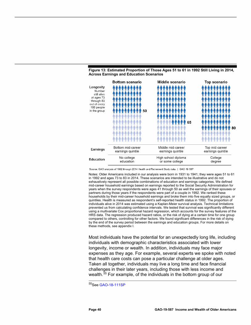
Page 40 GAO-19-587 Income and Wealth of Older Americans
Figure 13: Estimated Proportion of Those Ages 51 to 61 in 1992 Still Living in 2014, Across Earnings and Education Scenarios
Notes: Older Americans included in our analysis were born in 1931 to 1941; they were ages 51 to 61 in 1992 and ages 73 to 83 in 2014. These scenarios are intended to be illustrative and do not exhaustively represent all possible combinations of education and earnings categories. We defined mid-career household earnings based on earnings reported to the Social Security Administration for years when the survey respondents were ages 41 through 50 as well the earnings of their spouses or partners during those years if the respondents were part of a couple in 1992. We ranked these households by their mid-career household earnings and broke them into five equally sized groups, or quintiles. Health is measured as respondent’s self-reported health status in 1992. The proportion of individuals alive in 2014 was estimated using a Kaplan-Meier survival analysis. Technical limitations prevented us from calculating confidence intervals. We tested that survival was significantly different using a multivariate Cox proportional hazard regression, which accounts for the survey features of the HRS data. The regression produced hazard ratios, or the risk of dying at a certain time for one group compared to others, controlling for other factors. We found significant differences in the risk of dying by the end of the survey period between the earnings and education groups. For more details on these methods, see appendix I.
Most individuals have the potential for an unexpectedly long life, including individuals with demographic characteristics associated with lower longevity, income or wealth. In addition, individuals may face major expenses as they age. For example, several experts we spoke with noted that health care costs can pose a particular challenge at older ages. Taken all together, individuals may live a long time and face financial challenges in their later years, including those with less income and wealth.55 For example, of the individuals in the bottom group of our 55See GAO-18-111SP
Page 41 GAO-19-587 Income and Wealth of Older Americans
scenarios illustrating the effects of earnings and education on longevity, an estimated 50 percent were still alive in 2014. Should these individuals not have DC accounts or have little in them, or should they have little to no DB pension benefits, they may have to rely primarily on Social Security (which itself faces financing difficulties) or safety net programs.
Using HRS data and following the same households over time, we examined how income and wealth distributions changed and found that, in general, disparities in income decreased while disparities in wealth persisted among a cohort of older Americans as they aged (see text box for more information on our analysis).56 Households with the top 20 percent of mid-career earnings saw larger drops in income than households in other mid-career earnings groups, decreasing income disparities overall. During the same time period, the amount of wealth held by most households remained steady and wealth disparities persisted. We also found important differences in the distribution of income and wealth among households by race and ethnicity and education level.
Analyzing Income and Wealth for Households Over Time We analyzed Health and Retirement Study (HRS) data to estimate how income and wealth distributions changed as a particular cohort of older Americans aged over time. We analyzed income, wealth, and select financial resources for the same group of survey respondents (heads of households) or their spouses or partners who responded to the survey in 1992 and were still alive and responded in 2014, which is the most recent year for which the data are complete. We defined wealth as net worth. Data limitations prevented us from producing estimates of the present value of future income expected from Social Security or defined benefit pensions. The heads of households we analyzed were from the original HRS cohort and were born in 1931 to 1941. If neither the head of household or the spouse or partner interviewed in 1992 was still alive in 2014, their household was not included in our sample. As a nationally representative longitudinal survey, the HRS allows us to follow the same set of Americans from their 50s through the remainder of their lives; these household heads or their spouses or partners had reached their 70s or early 80s by 2014, allowing us to estimate how income and assets changed for the households as they progressed through retirement. We are reporting medians, as our analysis indicated that means were not consistently reliable. Appendix VI contains additional figures examining how assets and income changed for households headed by individuals in HRS’ “War Babies” cohort, who were born from 1942 through 1947. For our analysis, we divided older households in the data into five equally sized quintiles, or earnings groups, based on the number of households and their mid-career
56We followed households from 1992 to 2014, when heads of households were roughly in their 50s to when they or their spouses were in their 70s or early 80s. For the purposes of this analysis, we defined wealth as net worth.
While Income Disparities Declined As a Cohort of Older Americans Aged and Worked Less, Disparities in Wealth Persisted
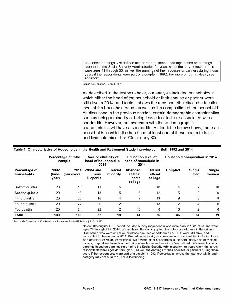
Page 42 GAO-19-587 Income and Wealth of Older Americans
household earnings. We defined mid-career household earnings based on earnings reported to the Social Security Administration for years when the survey respondents were ages 41 through 50, as well the earnings of their spouses or partners during those years if the respondents were part of a couple in 1992. For more on our analysis, see appendix I.
Source: GAO analysis. | GAO-19-587
As described in the textbox above, our analysis included households in which either the head of the household or their spouse or partner were still alive in 2014, and table 1 shows the race and ethnicity and education level of the household head, as well as the composition of the household. As discussed in the previous section, certain demographic characteristics, such as being a minority or being less educated, are associated with a shorter life. However, not everyone with these demographic characteristics will have a shorter life. As the table below shows, there are households in which the head had at least one of these characteristics and lived into his or her 70s or early 80s.
Table 1: Characteristics of Households in the Health and Retirement Study Interviewed in Both 1992 and 2014
Percentage of total sample
Race or ethnicity of head of household in
2014
Education level of head of household in
2014
Household composition in 2014
Percentage of households
1992 (base year)
2014 (survivors)
White and non-
Hispanic
Racial minority
Attended at least
some college
Did not attend
college
Coupled Single men
Single women
Bottom quintile 20 16 11 5 5 10 4 2 10 Second quintile 20 18 13 5 6 12 5 3 9 Third quintile 20 20 16 4 7 13 9 3 8 Fourth quintile 20 22 20 2 10 13 12 4 6 Top quintile 20 24 22 2 16 8 16 2 6 Total 100 100 82 18 44 56 46 14 39
Source: GAO analysis of 2014 Health and Retirement Study (HRS) data. | GAO-19-587
Notes: The original HRS cohort included survey respondents who were born in 1931-1941 and were ages 73 through 83 in 2014. We analyzed the demographic characteristics of those in the original HRS cohort who were still alive, or whose spouses or partners as of 1992 were still alive, and responded to the survey in 2014. We defined minority as someone who is non-white, including those who are black or Asian, or Hispanic. We divided older households in the data into five equally sized groups, or quintiles, based on their mid-career household earnings. We defined mid-career household earnings based on earnings reported to the Social Security Administration for years when the survey respondents were ages 41 through 50, as well the earnings of their spouses or partners during those years if the respondents were part of a couple in 1992. Percentages across the total row within each category may not sum to 100 due to rounding.
Page 43 GAO-19-587 Income and Wealth of Older Americans
We analyzed HRS data and found that household income declined as heads of households born from 1931 through 1941 and their spouses or partners aged, with decreased earnings from work contributing to the decline as people retired.57 Those households that had the highest mid-career earnings—those in the top earnings group—experienced the largest declines in income from 1992 when the heads of household were ages 51 to 61 to 2014 when the surviving heads of household or their spouses or partners were ages 73 to 83 (see fig. 14).58 For example, estimated median income for the top earnings group decreased by 53 percent, from about $121,000 in 1992 to about $57,000 in 2014. In comparison, for those with the lowest mid-career earnings—those in the bottom earnings group—estimated median income declined by 36 percent, from about $28,000 to about $18,000 over this same period.59
57 Appendix VI presents additional figures on how the estimated income and wealth of individuals born in 1942 through 1947, known as HRS’s “War Babies” cohort, changed as these individuals aged. 58As explained above, our sample included heads of households and their spouses or partners who responded to the HRS survey in 1992 and were still alive in 2014. Our sample included the spouse or partner who responded to the survey in 1992, even if the head of household was no longer alive in 2014. The age of spouses or partners may have been outside the age range of the heads of households. 59All values presented in this section of the report are in real 2016 dollars. Throughout this section, we present data on the change in the median value, not the median change.
Income Disparities Decreased Overall as Higher-Earning Households in Our Cohort saw Drops in Income
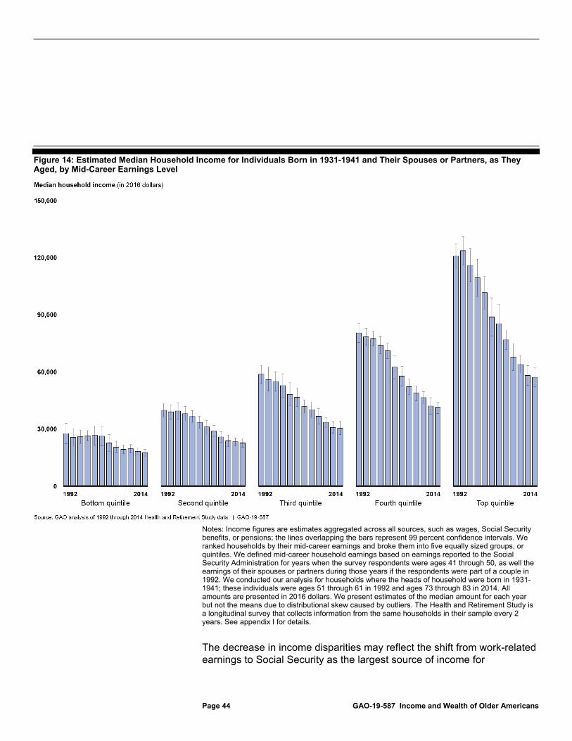
Page 44 GAO-19-587 Income and Wealth of Older Americans
Figure 14: Estimated Median Household Income for Individuals Born in 1931-1941 and Their Spouses or Partners, as They Aged, by Mid-Career Earnings Level
Notes: Income figures are estimates aggregated across all sources, such as wages, Social Security benefits, or pensions; the lines overlapping the bars represent 99 percent confidence intervals. We ranked households by their mid-career earnings and broke them into five equally sized groups, or quintiles. We defined mid-career household earnings based on earnings reported to the Social Security Administration for years when the survey respondents were ages 41 through 50, as well the earnings of their spouses or partners during those years if the respondents were part of a couple in 1992. We conducted our analysis for households where the heads of household were born in 1931-1941; these individuals were ages 51 through 61 in 1992 and ages 73 through 83 in 2014. All amounts are presented in 2016 dollars. We present estimates of the median amount for each year but not the means due to distributional skew caused by outliers. The Health and Retirement Study is a longitudinal survey that collects information from the same households in their sample every 2 years. See appendix I for details.
The decrease in income disparities may reflect the shift from work-related earnings to Social Security as the largest source of income for
Page 45 GAO-19-587 Income and Wealth of Older Americans
households in the top 20 percent, indicating the possible transition from working to retirement. More specifically, in 1992, 94 percent of households in the top mid-career earnings group had work-related earnings, which contributed the largest amount to their income. By 2014, only 25 percent of the top earnings group still had work-related earnings, and Social Security provided the highest median value of all income sources.60 Among households in the bottom mid-career earnings group, 68 percent had work-related earnings in 1992, and 15 percent continued to have work-related earnings in 2014. Similarly, work-related earnings provided the greatest source of income for these households in 1992, and Social Security provided the highest median value of all income sources for these households in 2014. However, concerns about retirement insecurity for those with lower earnings may remain. Social Security is progressive, meaning it replaces a higher percentage of income for those with lower earnings, but the formula for calculating Social Security benefits provides a higher benefit amount to those with higher lifetime earnings. In addition, those households with higher mid-career earnings maintained relatively higher income in retirement, perhaps due to their having higher levels of other types of non-wage income after retiring. For example, in 2014, a significantly greater percentage of households in the top two earnings groups had income from employer-sponsored retirement accounts compared to those in the bottom earnings groups, although households may not be consistent in how they spend down these funds.61
60While this analysis focused on changes in household income over time, our cross-sectional analysis of SCF data discussed previously found that, among all sources of income and wealth, assets excluding retirement accounts, a home, and the value of a household’s vehicle(s) provided the most value, on average, for households in the top quintile. These assets were also higher in amount, on average, than the present value of future income from Social Security and DB pensions. 61Unlike Social Security or DB pension income, individuals manage their withdrawals from defined contribution accounts and IRAs and determine how to spend down their account balances. For example, individuals may spend down their defined contribution account balances through lump sum payments, programmed withdrawals, annuities, or possibly some combination thereof. Or, they may choose to hold their account balances in reserve, withdrawing only what the law requires. As a result, some households may use their account balances in response to short-term spending needs rather than using their savings as an ongoing source of income.

Page 46 GAO-19-587 Income and Wealth of Older Americans
We analyzed HRS data from 1992 to 2014—when heads of households were in roughly their 50s to when they were in their 70s or early 80s—and found that for most households, the level of wealth was relatively consistent as they aged, and disparities in wealth persisted over time. As shown in figure 15, wealth remained relatively steady for households in the bottom three mid-career earnings groups over the time period we examined while households in the top two mid-career earnings groups experienced larger fluctuations in wealth. More specifically, households in the top two earnings groups saw their wealth increase overall from 1992 to 2014. However, while wealth increased from 1992 to 2006, this was followed by declines in wealth from 2006 to 2014.62 Looking at the overall time period of our analysis, wealth disparities persisted between households in the top earnings groups and households in the bottom earnings groups. For example, in 1992, households in the bottom 20 percent had estimated median wealth of about $93,000 while households in the top 20 percent had estimated median wealth of about $432,000, a difference of about $339,000 (or the top had about 4.6 times the median wealth of the bottom). In 2014, households in the bottom 20 percent had estimated median wealth of about $66,000 while households in the top 20 percent had estimated median wealth of about $539,000, a difference of about $473,000 (or the top had about 8.2 times the median wealth of the bottom). Other researchers have found that that some households may not spend down their wealth as much during retirement due to factors including a generally higher propensity to save, a desire to leave bequests, and the desire to self-insure against medical costs.63
62The overall increase in wealth from 1992 to 2014 was not statistically significant. The increase in wealth from 1992 to 2006 for households in the top 20 percent was statistically significant, and declines in wealth from 2006 to 2014 were not statistically significant. 63Poterba et al., “Longitudinal Determinants”; Sudipto Banerjee, “Asset Decumulation or Asset Preservation? What Guides Retirement Spending?,” Employee Benefit Research Institute Issue Brief No. 447 (2018); and Karen Smith, Mauricio Soto and Rudolph G. Penner, “How Seniors Change Their Asset Holdings During Retirement,” Center for Retirement Research at Boston College Working Paper, vol. 2009, no. 31 (2009).
Wealth Remained Steady for Most Households in Our Cohort, and Disparities Persisted
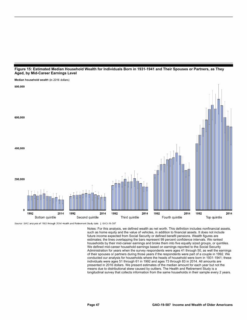
Page 47 GAO-19-587 Income and Wealth of Older Americans
Figure 15: Estimated Median Household Wealth for Individuals Born in 1931-1941 and Their Spouses or Partners, as They Aged, by Mid-Career Earnings Level
Notes: For this analysis, we defined wealth as net worth. This definition includes nonfinancial assets, such as home equity and the value of vehicles, in addition to financial assets. It does not include future income expected from Social Security or defined benefit pensions. Wealth figures are estimates; the lines overlapping the bars represent 99 percent confidence intervals. We ranked households by their mid-career earnings and broke them into five equally sized groups, or quintiles. We defined mid-career household earnings based on earnings reported to the Social Security Administration for years when the survey respondents were ages 41 through 50, as well the earnings of their spouses or partners during those years if the respondents were part of a couple in 1992. We conducted our analysis for households where the heads of household were born in 1931-1941; these individuals were ages 51 through 61 in 1992 and ages 73 through 83 in 2014. All amounts are presented in 2016 dollars. We present estimates of the median amount for each year but not the means due to distributional skew caused by outliers. The Health and Retirement Study is a longitudinal survey that collects information from the same households in their sample every 2 years.
Page 48 GAO-19-587 Income and Wealth of Older Americans
Households in the top 20 percent of mid-career earnings had greater participation in retirement accounts (see sidebar) and increased home equity relative to other households, which may have contributed to wealth disparities over the time period of our analysis.
• Retirement Accounts.64 Among households that had retirement accounts, the median value of retirement accounts increased for all of our income groups (see fig. 16); however, the continued wealth disparities between higher- and lower-earning households may be due to significant differences in the value of retirement accounts and in household participation. The value of retirement accounts for households in the top and bottom earnings groups increased substantially between 1992 and 2014 (a 93 percent and 138 percent increase, respectively). Some of the increase in retirement account balances over time may be due to contributions to DC plans and IRAs during years in which individuals worked, as well as waiting until age 70 ½, when many individuals are required to take minimum distributions from their IRAs.65 Despite this potential for gains in account balances across the distribution, disparities still exist. In 2014, among households that had retirement accounts, we estimated that households in the top 20 percent had about three times more in their retirement accounts compared to households in the bottom 20 percent (about $176,000 compared to about $54,000). Higher-earning households may not spend down their retirement account balances as much in retirement whereas lower-earning households may have spent down all or part of their account balances. In addition to having more in their retirement accounts, a greater percentage of households in the top earnings group had retirement accounts compared to households in the bottom earnings group. For example, in 2014, an estimated 69 percent of households in the top 20 percent had
64We included employer-sponsored defined contribution plans, individual retirement accounts (IRAs), and Keogh accounts when calculating retirement account balances. This measure does not include any future income streams from DB pension plans. 65James M. Poterba “Retirement Security in an Aging Population,” The American Economic Review, Vol. 104, No. 5 (2014) and Smith et al. (2009).
Shifts in the Type of Retirement Plans Over the past 40 years, there has been a significant shift in the type of retirement plans offered by private-sector employers, who have increasingly moved away from offering defined benefit plans to offering defined contribution plans (e.g., 401(k)s) as their primary retirement plan. In addition, there has been a significant increase in the amount of assets held in defined contribution plans and individual retirement accounts (IRAs). In the private sector, total assets in defined contribution plans and IRAs far exceed those in defined benefit plans. As a result, individuals have greater responsibility for making investment decisions. Given the shift away from defined benefit plans, our analysis on retirement accounts focused on defined contribution accounts and IRAs, and Keogh accounts (for self-employed individuals). In addition, we focused on those who had these retirement accounts rather than all households in order to better capture the experience of those who had these accounts. Source: GAO analysis. | GAO-19-587
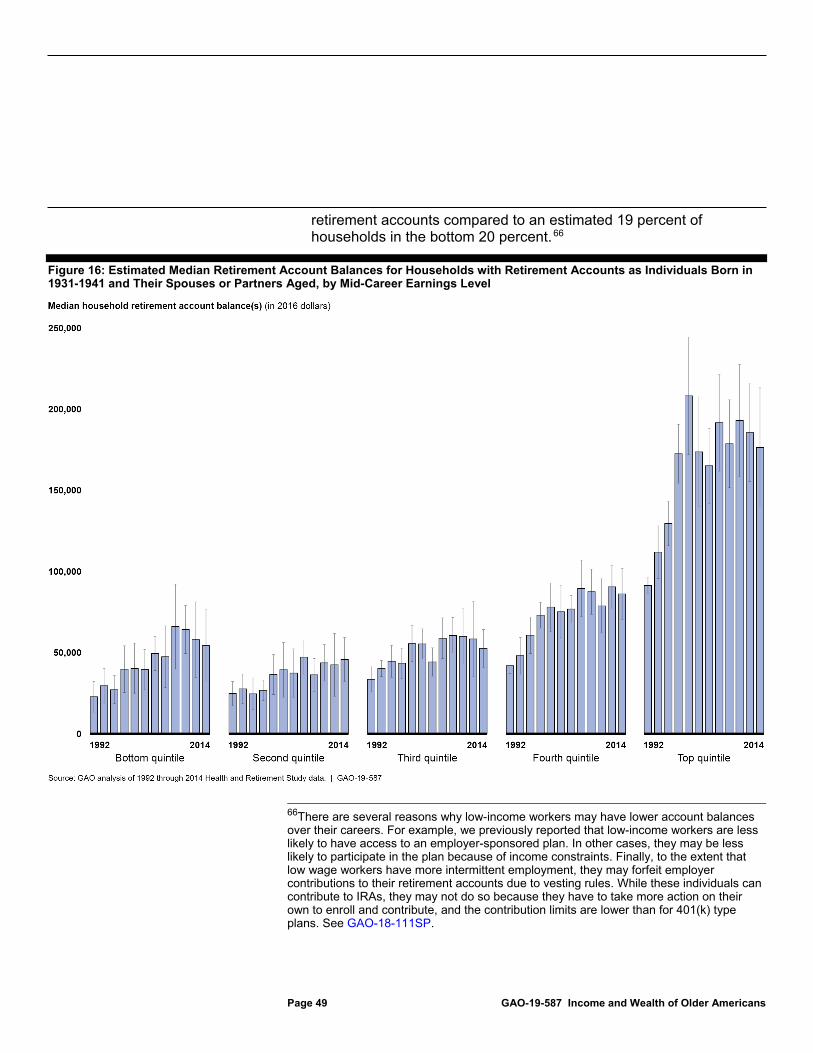
Page 49 GAO-19-587 Income and Wealth of Older Americans
retirement accounts compared to an estimated 19 percent of households in the bottom 20 percent.66
Figure 16: Estimated Median Retirement Account Balances for Households with Retirement Accounts as Individuals Born in 1931-1941 and Their Spouses or Partners Aged, by Mid-Career Earnings Level
66There are several reasons why low-income workers may have lower account balances over their careers. For example, we previously reported that low-income workers are less likely to have access to an employer-sponsored plan. In other cases, they may be less likely to participate in the plan because of income constraints. Finally, to the extent that low wage workers have more intermittent employment, they may forfeit employer contributions to their retirement accounts due to vesting rules. While these individuals can contribute to IRAs, they may not do so because they have to take more action on their own to enroll and contribute, and the contribution limits are lower than for 401(k) type plans. See GAO-18-111SP.
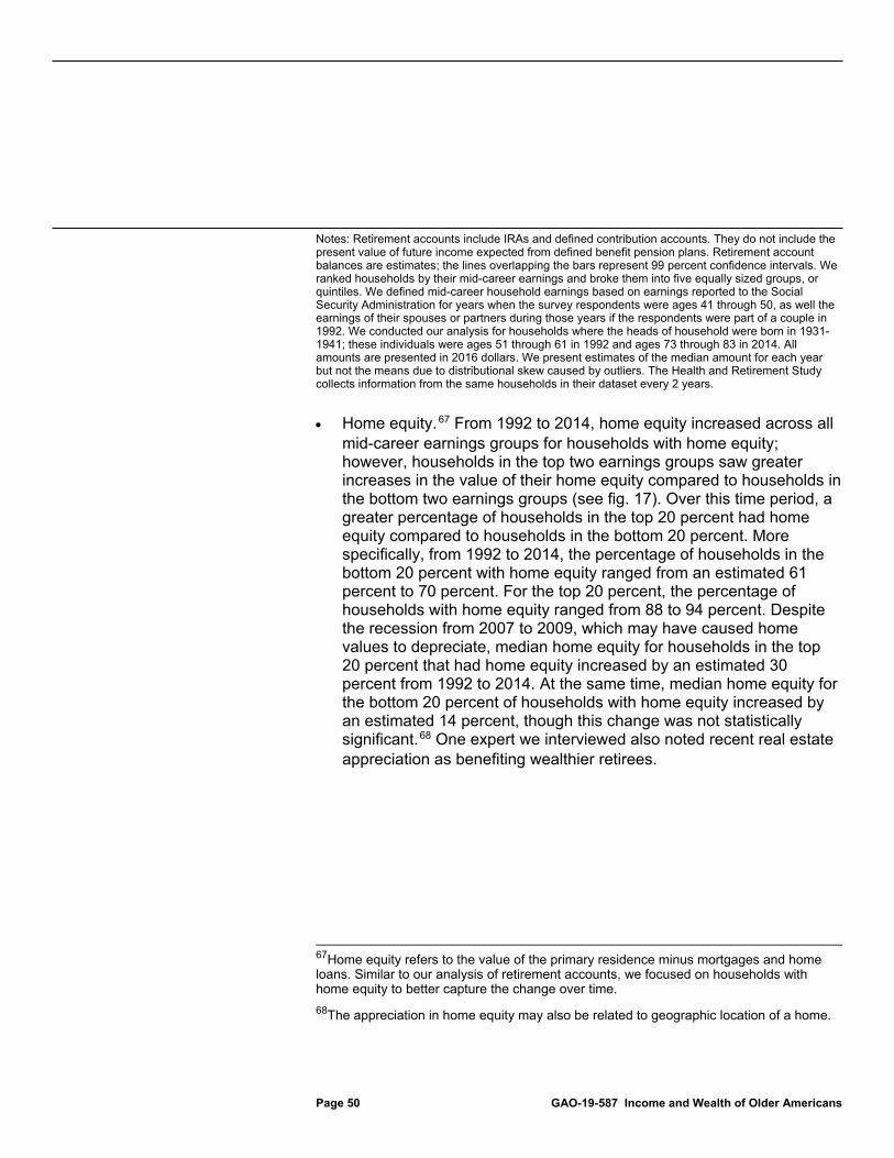
Page 50 GAO-19-587 Income and Wealth of Older Americans
Notes: Retirement accounts include IRAs and defined contribution accounts. They do not include the present value of future income expected from defined benefit pension plans. Retirement account balances are estimates; the lines overlapping the bars represent 99 percent confidence intervals. We ranked households by their mid-career earnings and broke them into five equally sized groups, or quintiles. We defined mid-career household earnings based on earnings reported to the Social Security Administration for years when the survey respondents were ages 41 through 50, as well the earnings of their spouses or partners during those years if the respondents were part of a couple in 1992. We conducted our analysis for households where the heads of household were born in 1931-1941; these individuals were ages 51 through 61 in 1992 and ages 73 through 83 in 2014. All amounts are presented in 2016 dollars. We present estimates of the median amount for each year but not the means due to distributional skew caused by outliers. The Health and Retirement Study collects information from the same households in their dataset every 2 years.
• Home equity.67 From 1992 to 2014, home equity increased across all mid-career earnings groups for households with home equity; however, households in the top two earnings groups saw greater increases in the value of their home equity compared to households in the bottom two earnings groups (see fig. 17). Over this time period, a greater percentage of households in the top 20 percent had home equity compared to households in the bottom 20 percent. More specifically, from 1992 to 2014, the percentage of households in the bottom 20 percent with home equity ranged from an estimated 61 percent to 70 percent. For the top 20 percent, the percentage of households with home equity ranged from 88 to 94 percent. Despite the recession from 2007 to 2009, which may have caused home values to depreciate, median home equity for households in the top 20 percent that had home equity increased by an estimated 30 percent from 1992 to 2014. At the same time, median home equity for the bottom 20 percent of households with home equity increased by an estimated 14 percent, though this change was not statistically significant.68 One expert we interviewed also noted recent real estate appreciation as benefiting wealthier retirees.
67Home equity refers to the value of the primary residence minus mortgages and home loans. Similar to our analysis of retirement accounts, we focused on households with home equity to better capture the change over time. 68The appreciation in home equity may also be related to geographic location of a home.
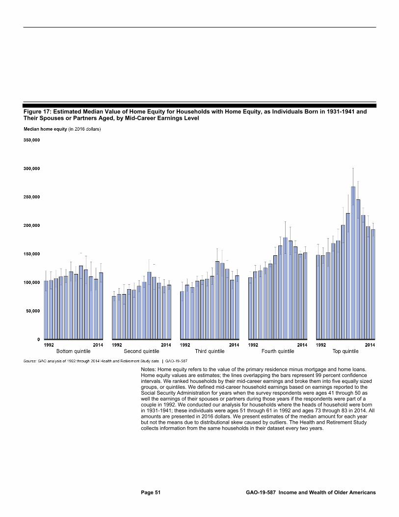
Page 51 GAO-19-587 Income and Wealth of Older Americans
Figure 17: Estimated Median Value of Home Equity for Households with Home Equity, as Individuals Born in 1931-1941 and Their Spouses or Partners Aged, by Mid-Career Earnings Level
Notes: Home equity refers to the value of the primary residence minus mortgage and home loans. Home equity values are estimates; the lines overlapping the bars represent 99 percent confidence intervals. We ranked households by their mid-career earnings and broke them into five equally sized groups, or quintiles. We defined mid-career household earnings based on earnings reported to the Social Security Administration for years when the survey respondents were ages 41 through 50 as well the earnings of their spouses or partners during those years if the respondents were part of a couple in 1992. We conducted our analysis for households where the heads of household were born in 1931-1941; these individuals were ages 51 through 61 in 1992 and ages 73 through 83 in 2014. All amounts are presented in 2016 dollars. We present estimates of the median amount for each year but not the means due to distributional skew caused by outliers. The Health and Retirement Study collects information from the same households in their dataset every two years.
Page 52 GAO-19-587 Income and Wealth of Older Americans
Significant differences in income and wealth associated with race and ethnicity, as well as education levels, continued as households aged, according to our analysis of heads of households and their spouses or partners as they aged from roughly their 50s to their 70s or early 80s using 1992 through 2014 HRS data.
Non-Hispanic, white households in the bottom 40 percent of mid-career earnings had higher estimated median incomes, and non-Hispanic, white households across the mid-career earnings distribution generally had greater wealth, than minority households.69
• In terms of income, the gap between non-minority and minority households in the bottom 40 percent persisted even as median income decreased overall for households as they aged. For example, we estimated that, in 1992, non-Hispanic, white households in the bottom 20 percent had about $20,000 more in income than minority households. The income disparity was smaller (about $9,700) in 2014, but still remained.70
• In terms of wealth, non-Hispanic, white households had persistently higher wealth compared to minority households across all levels of the mid-career earnings distribution. For example, among the bottom 20 percent of households, in 1992, non-Hispanic, white households had about $138,000 more in estimated median wealth than minority households. While this difference decreased to about $119,000 in 2014, the wealth difference remained. Similarly, for the top 20 percent of households, in 1992, non-Hispanic, white households had about $170,000 more in estimated median wealth than minority households, and, in 2014, the wealth disparity increased to about $294,000.
69We defined minority as someone who is non-white, including those who are black or Asian, or Hispanic. For the purposes of this analysis, the data were insufficient for breaking out results by specific race and ethnicity categories, so we were unable to present data on minority subgroups. As a result, there may be other wealth and income disparities not captured by our analysis. Additional estimates from this analysis are presented in appendix III. 70We did not find significant differences in income between minority and non-minority households at the higher end of the mid-career earnings distribution; for our analysis, the number of minority households in this group was too small to draw conclusions.
Race and Ethnicity and Education Were Factors in Persistent Income and Wealth Disparities As Households in Our Cohort Aged
Race and Ethnicity
Page 53 GAO-19-587 Income and Wealth of Older Americans
Households headed by someone with at least some college education generally had higher median incomes and more wealth than households headed by someone who did not attend college.
• Income disparities existed across the mid-career earnings distribution from 1992 to 2014. For example, we estimated that, in 1992, households in the top 20 percent with heads who attended college had about $44,000 more in income compared to households in the top 20 percent with heads who did not attend college. We estimated that, in 2014, households with heads in the top 20 percent who had attended college still had greater income, though the difference was smaller (about $25,000). Similarly, heads of households in the bottom 20 percent who had attended some college had more income than heads of household who had not. For example, in 1992, households with heads who had attended some college had about $31,000 more in income than households with heads who had not, and that difference decreased to $9,700 in 2014.71
• Wealth disparities generally existed across the mid-career earnings distribution over time. For example, in 1992, households in the top 20 percent with heads who had attended some college had about $166,000 more in estimated median wealth compared to households in the top 20 percent with heads who did not attend college. In 2014, the difference in estimated median wealth between these same groups was about $386,000. Similarly, households in the bottom 20 percent with heads who had attended some college had greater median wealth than households in the bottom 20 percent with heads who had not attended college. For example, we estimated that, in 1992, households in the bottom 20 percent with heads who attended college had about $176,000 more in wealth than heads who had not. In 2014, the difference in median wealth between these groups was about $120,000.72 Our findings are consistent with those of other researchers, who found that educational attainment was an important determinant of wealth at age 65, and that it was strongly correlated with wealth even after controlling for lifetime earnings.73
71The difference in median income in 2014 was not statistically significant. 72This difference was not statistically significant. 73Poterba et al., “Longitudinal Determinants.”
Education

Page 54 GAO-19-587 Income and Wealth of Older Americans
We provided a draft of this report to the Department of Labor, the Department of the Treasury, the Internal Revenue Service, and the Social Security Administration for review and comment. While none of the agencies provided official comments, the Department of Labor and Social Security Administration provided technical comments, which we incorporated as appropriate.
As agreed with your office, unless you publicly announce the contents of this report earlier, we plan no further distribution until 30 days from the report date. At that time, we will send copies to the Secretary of Labor, the Secretary of the Treasury, the Commissioner of the Internal Revenue Service, and the Commissioner of the Social Security Administration. In addition, the report will be available at no charge on the GAO website at http://www.gao.gov.
If you or your staff have any questions about this report, please contact me at (202) 512-7215 or [email protected]. Contact points for our Offices of Congressional Relations and Public Affairs may be found on the last page of this report. GAO staff who made key contributions to this report are listed in appendix VIII.
Sincerely yours,
Charles A. Jeszeck Director, Education, Workforce, and Income Security Issues
Agency Comments
Appendix I: Objectives, Scope, and Methodology
Page 55 GAO-19-587 Income and Wealth of Older Americans
To determine how growing disparities in the distributions of income and wealth affect older Americans, we examined (1) the distributions of income and wealth among all older Americans over time; (2) the association between income, wealth, and longevity among older Americans; and (3) how the distributions of income and wealth have changed over time for a cohort of individuals as they aged. This appendix provides a detailed account of the data sources used to answer these questions and the analyses we conducted.
The appendix is organized into three sections. Section I describes how we reviewed literature relevant to this report’s objectives and provides information on the interviews we conducted. Section II describes the information sources and methods we used to analyze the distributions of income and wealth among all older Americans over time. Section III describes the information sources and methods we used to analyze how income and wealth among older Americans are associated with longevity, and how the distributions of income and wealth changed as a cohort of individuals aged.
For the purposes of our analysis, we defined wealth to be a household’s net worth—that is, total assets minus total debt. Net worth is a measure often used by researchers studying retirement security. Older Americans may have other future retirement resources, such as the present value of future income expected from defined benefit (DB) pension plans and Social Security.
We supplemented our data analysis with a literature review and interviewed researchers to identify appropriate background information and context.
We had two primary methods for identifying literature to include in our literature review: a snowball technique and a database search. To apply the snowball technique, we first identified possible relevant literature by examining the studies cited in our 2016 report examining the relationship between Social Security benefits and longevity.1 Then we reviewed the citations included in those studies. Finally, we reviewed relevant literature
1GAO, Retirement Security: Shorter Life Expectancy Reduces Projected Lifetime Benefits for Lower Earners, GAO-16-354 (Washington, D.C.: Mar. 25, 2016).
Appendix I: Objectives, Scope, and Methodology
Overview
Section I: Literature Review and Interviews
Appendix I: Objectives, Scope, and Methodology
Page 56 GAO-19-587 Income and Wealth of Older Americans
included in a weekly report called “Current Awareness in Aging Report,” produced by the Center for Demography of Health and Aging at the University of Wisconsin-Madison, which includes a comprehensive list of recently issued materials relating to aging, including retirement security. We compiled relevant citations across these sources and analyzed abstracts to identify working papers, journal articles, and reports that required further review. We identified reports for inclusion based on whether they provided insight into the following relationships:
• As older Americans age, the relationship between
• income and expenses,
• wealth and expenses, and
• income and wealth.
• For older Americans, how income and/or wealth inequality are (1) related to the topics below and (2) how, if at all, these relationships have changed over time or generations:
• Longevity
• Health status
• Gender
• Race and ethnicity
• Education
• Rural vs urban locations
• Role of inequality (income, wealth, longevity) in reliance on federal income security programs among older Americans
To complement the snowball technique search, we also conducted a database search. We searched the Proquest database EconLit for scholarly journals and working papers for a 5-year span, from 2013 through 2018, that matched keywords related to our criteria for relevance.
We took additional steps to enhance the robustness of our results. We solicited recommendations for literature from GAO stakeholders, agency officials, and contacts at the Congressional Research Service and Congressional Budget Office and added these recommendations to our list for consideration. During interviews with experts, we discussed contrary opinions and findings in the research and requested full citations as needed. We also attended retirement security events and reviewed news clippings for references to contrary opinions or findings in breaking
Appendix I: Objectives, Scope, and Methodology
Page 57 GAO-19-587 Income and Wealth of Older Americans
research. Finally, an economist reviewed the methods and reliability of all studies.
We included 26 out of 34 articles from the snowball technique search and expert recommendations and an additional 3 out of 160 articles from the database search (the database search identified some of the same articles as the snowball technique search). These 29 articles that best matched our criteria for inclusion were the articles we reviewed.
We also identified and interviewed nine researchers whose work was relevant to our objectives and interviewed them in order to identify researchers’ explanations and theories about the relationships between inequality and longevity, health status, gender, education, and race and ethnicity. To select these researchers, we considered their areas of expertise; whether they worked for a federal agency, university, or other type of organization; and their ideological perspective, if known.
This section describes the two main data sources we used to analyze trends in the distribution of income and wealth among all older Americans: the Survey of Consumer Finances (SCF) and the Financial Accounts of the United States (FA).
To examine the distributions of income and wealth among all older Americans over time, we used 1989 through 2016 data from the SCF. The SCF is a triennial survey of household assets and income from the Board of Governors of the Federal Reserve System (Federal Reserve) and asks households detailed questions about their income—including pension benefits—and assets—including amounts in retirement accounts. The survey also asks about debt and demographic information, among other topics. A different sample of households was used for each year in our analysis. These data allow for comparison of the experiences of same-age households at different points in time.
Section II: Analyzing Trends over Time in the Distribution of Income and Wealth among All Older Americans
Data Sources
Survey of Consumer Finances
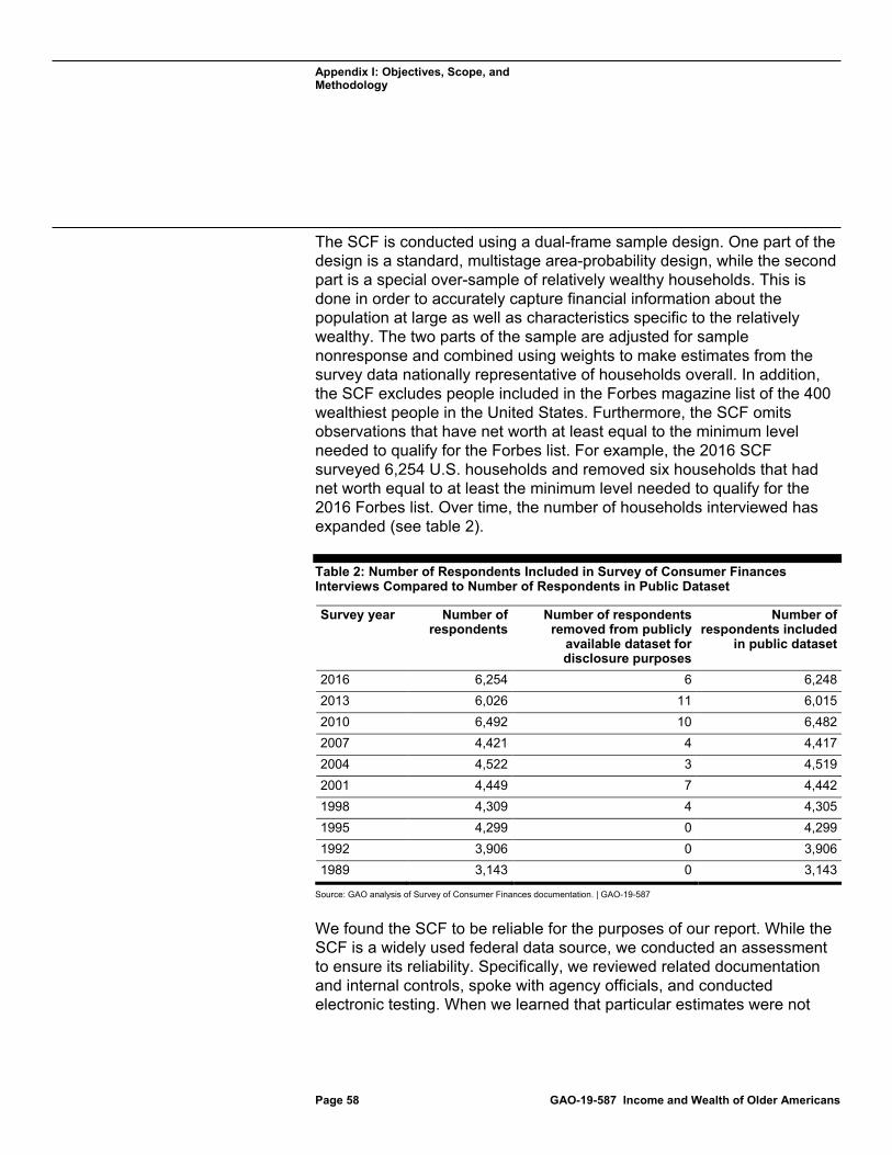
Appendix I: Objectives, Scope, and Methodology
Page 58 GAO-19-587 Income and Wealth of Older Americans
The SCF is conducted using a dual-frame sample design. One part of the design is a standard, multistage area-probability design, while the second part is a special over-sample of relatively wealthy households. This is done in order to accurately capture financial information about the population at large as well as characteristics specific to the relatively wealthy. The two parts of the sample are adjusted for sample nonresponse and combined using weights to make estimates from the survey data nationally representative of households overall. In addition, the SCF excludes people included in the Forbes magazine list of the 400 wealthiest people in the United States. Furthermore, the SCF omits observations that have net worth at least equal to the minimum level needed to qualify for the Forbes list. For example, the 2016 SCF surveyed 6,254 U.S. households and removed six households that had net worth equal to at least the minimum level needed to qualify for the 2016 Forbes list. Over time, the number of households interviewed has expanded (see table 2).
Table 2: Number of Respondents Included in Survey of Consumer Finances Interviews Compared to Number of Respondents in Public Dataset
Survey year Number of respondents
Number of respondents removed from publicly
available dataset for disclosure purposes
Number of respondents included
in public dataset
2016 6,254 6 6,248 2013 6,026 11 6,015 2010 6,492 10 6,482 2007 4,421 4 4,417 2004 4,522 3 4,519 2001 4,449 7 4,442 1998 4,309 4 4,305 1995 4,299 0 4,299 1992 3,906 0 3,906 1989 3,143 0 3,143
Source: GAO analysis of Survey of Consumer Finances documentation. | GAO-19-587
We found the SCF to be reliable for the purposes of our report. While the SCF is a widely used federal data source, we conducted an assessment to ensure its reliability. Specifically, we reviewed related documentation and internal controls, spoke with agency officials, and conducted electronic testing. When we learned that particular estimates were not
Appendix I: Objectives, Scope, and Methodology
Page 59 GAO-19-587 Income and Wealth of Older Americans
reliable for our purposes, or had sample sizes too small to produce reliable estimates, we did not use them.
Nonetheless, the SCF and other surveys that are based on self-reported data are subject to nonsampling error, including the ability to get information about all sample cases; difficulties of definition; differences in the interpretation of questions; and errors made in collecting, recording, coding, and processing data. These nonsampling errors can influence the accuracy of information presented in the report, although the magnitude of their effect is not known.
Estimates from the SCF are also subject to some sampling error since, for any given year, the sample is one of a large number of random samples that might have been drawn. Since each possible sample could have provided different estimates, we express our confidence in the precision of the sample results as 95 percent confidence intervals. These intervals would contain the actual population values for 95 percent of the samples that could have been drawn. In this report, we present 95 percent confidence intervals alongside the numerical estimates that were produced using SCF data. All financial figures using the SCF data are in 2016 dollars.
We supplemented the SCF data with data from the Financial Accounts of the United States (FA). The FA include data on transactions and levels of financial assets, and liabilities, by sector and financial instrument; balance sheets, including changes in net worth, for households and nonprofit organizations, nonfinancial corporate businesses, and nonfinancial noncorporate businesses; Integrated Macroeconomic Accounts; and additional supplemental detail. These data provide an aggregate estimate of DB pension entitlements (or liabilities, as the FA refer to them), which can be apportioned across SCF respondents (see detailed explanation below).
This section describes the analysis that we conducted using the SCF and FA to analyze trends in income and wealth over time for all older Americans.
We chose to look at household-level resources because couples may pool their economic resources and the SCF asks some of its questions about resources for households. The Federal Reserve provides the underlying programming code for creating the variables presented in its publications. Where possible, we relied on variable definitions used for
Financial Accounts of the United States
Cross-Sectional Analysis
Key Definitions and Assumptions
Appendix I: Objectives, Scope, and Methodology
Page 60 GAO-19-587 Income and Wealth of Older Americans
Federal Reserve publications using the SCF. For example, we used the race or ethnicity of the household head, defined as either 1) white, non-Hispanic or 2) non-white or Hispanic (which we renamed “minority” for ease of reporting).2 We also relied on the Federal Reserve’s definitions for
• net worth, which we refer to as “wealth” in this report;
• retirement account balances (DC plans and IRAs);
• income from withdrawals from retirement accounts; and
• income from Social Security, pension, or disability benefits or annuities.
In other cases, we developed our own variables, based on the raw variables described in the SCF codebooks. For example:
• Older households: households in which the survey respondent or any spouse or partner were aged 55 or older. 3
• Household income: estimated total income by adding up all of the individual income components created by the Federal Reserve.
• Other assets: any other assets that are not retirement accounts, the present value of future income from Social Security or DB pensions, or the value of the household’s primary residence (if one is owned) or vehicles.
• Other income: any other income coming from a source besides wages; withdrawals from retirement accounts; and Social Security, pension, or disability benefits or annuities.
The SCF is a cross-sectional survey, meaning it presents a nationally representative “snapshot” for each survey wave rather than following the same households over time. To create an income distribution, we rank ordered older households by household income and then broke them into five even groups, or quintiles. The “top” refers to the top 20 percent of households in this ranking while the “bottom” refers to the bottom 20 percent of households. We repeated this exercise for each year of the data. While the households included in the SCF are different every survey
2Non-white or Hispanic would include those respondents who responded to being black/African-American non-Hispanic, Hispanic or Latino, or Other or Multiple Race. 3For purposes of data organization, the Federal Reserve considers the household head to be the male within a mixed-sex couple and the older individual within a single-sex couple.
Analysis Goals
Appendix I: Objectives, Scope, and Methodology
Page 61 GAO-19-587 Income and Wealth of Older Americans
year, we were able to examine how the distribution of income and wealth across older households changed over time. We used the same method to create wealth distributions, except we rank ordered households by net worth, one measure of wealth, instead of income.
To better understand increases in the top quintile, we also estimated the amount of income and wealth held among the top 10 percent, 5 percent, and 1 percent of households, when possible, for each survey year. 4 We also created distributions of income and wealth for other subcategories of older households. As with the analysis for all older households, we broke the subcategory population into quintiles. We estimated distributions of income and wealth for the following subcategories for each survey year:
• Households in which the head was white and non-Hispanic
• Households in which the head was a minority
• Coupled households
• Single men
• Single women
• Households in which the head attended at least some college
• Households in which the head did not attend college
For all older households, we also estimated the percentage of households in each survey year that had 1) wage income, 2) income from retirement account withdrawals or 3) income from Social Security, pension, or disability benefits or annuities, as well as the amount of income provided by each source. Similarly, we estimated the percentage of older households that had a retirement account (DC or IRA), owned their home, or owned a vehicle, as well as the value of each of these assets. To better understand the importance of these asset types across the wealth distribution, we also estimated the percentage of households that had a retirement account (DC or IRA) with a balance of at least a $100; owned a vehicle worth at least $100; or had home equity of at least $100. We also analyzed the percentage of households with retirement account balances by bands of $50,000.
4Our early analyses examined the distribution of income and wealth by deciles—that is, we created 10 equally sized groups, with the first containing the first 10 percent of the distribution, the second containing the next 10 percent of the distribution and so on. However, there were insufficient data to produce all of the estimates required for our analysis.
Appendix I: Objectives, Scope, and Methodology
Page 62 GAO-19-587 Income and Wealth of Older Americans
Additional sensitivity analysis included comparing a household’s location in the income distribution to its location in the wealth distribution for each survey year. We found that the vast majority of households were in the same quintile of the income and wealth distributions or were only one quintile apart. Very few households were in the bottom quintile for income and top quintile for wealth or vice-versa. From 1989 through 2016, the percentage of households who fit these two scenarios was always under 1 percent.
The literature on retirement adequacy emphasizes the importance of including measures of the value of future DB and Social Security benefits in measures of the wealth distribution. However, the SCF does not provide estimates of the present value of expected future DB and Social Security benefits. As a result, we did a separate analysis to estimate the present value of future income from DB and Social Security benefits using the SCF and FA data from the Federal Reserve, as well as life expectancy data from the Social Security Administration (SSA). In general, our analysis was done for respondents and spouses/partners separately at the individual level, and estimates were combined to create household totals. We generally followed methods presented in an 2016 paper entitled “Is the U.S. Retirement System Contributing to Rising Wealth Inequality?” by Devlin-Foltz, Henriques, and Sabelhaus (see bibliography for the full citation), but made some changes in the assumptions given our specific focus on older Americans.5
In order to estimate the present value of income expected from DB plans at the household-level, we started with the aggregate value of accrued DB benefits by survey year from the FA. Following Devlin-Foltz et al. (2016), we calculated aggregate DB pension entitlements as the portion of total pension entitlements not found in DC assets and annuities held in IRAs at life insurance companies. Then, we allocated aggregate DB entitlements across households in a series of steps, ultimately splitting the aggregate DB entitlements between SCF respondents who were already receiving benefits and those who were covered by DB plans but were not yet receiving benefits.
In the first step of the allocation, we estimated the present value of promised DB benefits for current DB beneficiaries. The present value of
5The authors continue to refine their methodology and we relied on recently available papers as a starting point for our analysis.
Estimating the Present Value of Social Security and Defined Benefit Pension Benefits
Appendix I: Objectives, Scope, and Methodology
Page 63 GAO-19-587 Income and Wealth of Older Americans
promised DB benefits for those already receiving benefits was based on the reported values for DB benefits in the SCF, life tables from SSA, and an assumed 3 percent real discount rate. After solving for the present value of promised DB benefits for those currently receiving benefits, we subtracted the total amount of DB benefits promised to current DB beneficiaries from the aggregate DB assets to solve for the share to be distributed to future DB beneficiaries. By doing this, we effectively assumed that current DB beneficiaries had first claim to DB pension assets. We allocated the remaining DB assets to future DB recipients by assigning each future DB beneficiary a share of the amount of the residual of aggregate DB entitlements (left over after current beneficiaries claimed their share) based on their earnings, the number of years they participated in a DB plan, their expected retirement age as stated in the SCF, and a 3 percent real discount rate.
We also estimated the present value of expected future Social Security benefits for current and future Social Security beneficiaries, using information from the SCF on Social Security benefits for current Social Security beneficiaries and earnings information for future Social Security beneficiaries.
With respect to current Social Security beneficiaries, we solved for the present value of Social Security benefits using annual Social Security benefits as reported in the SCF, life tables from SSA, and an assumed 3 percent real discount rate, consistent with our DB analysis. For future Social Security beneficiaries, we used current earnings or earnings from the longest job held as reported in the SCF as the basis for the Social Security benefit. Given that our analysis focused on older Americans, we assumed that future Social Security beneficiaries were close enough to retirement that the earnings information in the SCF provided a reasonable proxy for lifetime earnings. We created a monthly average of these earnings, which we used as a simplified version of the average indexed monthly earnings (AIME). We used these thresholds to compute something similar to the primary insurance amount (PIA) by assigning 90 percent of earnings up to the first bend point, 32 percent of earnings between the first and second bend points, and 15 percent of earnings between the second bend point and the monthly taxable maximum.6 We assumed everyone who was not yet receiving benefits but would in the future started collecting benefits at 62 or at their current age if older than
6These thresholds match the “bend points” used by the Social Security program.
Appendix I: Objectives, Scope, and Methodology
Page 64 GAO-19-587 Income and Wealth of Older Americans
62. We applied benefit rules associated with each individual’s birth year to the PIA as set by the Social Security Administration and made adjustments for spousal benefits. We estimated the present value of Social Security benefits for future beneficiaries using the estimated PIA, a retirement age of 62 or their current age if older than 62 and not yet receiving benefits, life tables from SSA, and a 3 percent real discount rate.
While adding these present value estimates to wealth better captures the totality of resources available to older Americans, our estimates of the present value of income from future DB and Social Security benefits are subject to uncertainty and should be interpreted with caution. For example, our estimates of the present value of DB benefits for future beneficiaries are not based on SCF respondent-reported expected DB benefits. Instead, we used the aggregate DB entitlements in the FA data and allocated that amount across households with DB plans. We followed this method, in part, because it appears that workers do not have a good understanding of their pension plan parameters and confuse DB benefits with other types of payouts in the SCF data, according to Devlin-Foltz et al. (2016).
Moreover, our estimates of the present value of Social Security benefits for future beneficiaries are not based on lifetime earnings since the SCF does not collect all of the inputs needed to project Social Security benefits for respondent-families. However, it is possible to get a sense of the distributional impact of Social Security by focusing on those near retirement in certain points in time.
A general limitation of our analysis of the present value of future income from DB pensions and Social Security is that our estimates rely on assumptions about life expectancy, real discount rates, and retirement ages, which are unlikely to hold for all households. As a result, we conducted some sensitivity analyses, particularly with respect to real discount rates and retirement ages.
For both the DB and Social Security sensitivity analyses, we varied the real discount rate given the uncertainty about future interest rates. In general, higher discount rates result in lower estimated present values, so our estimates of the present value of future DB and Social Security benefits are sensitive to the assumptions about the discount rate. This is especially important in the DB analysis, as changing the assumed discount rate affects the allocation of aggregate DB assets between current and future DB beneficiaries. For example, using a 2 percent real
Appendix I: Objectives, Scope, and Methodology
Page 65 GAO-19-587 Income and Wealth of Older Americans
discount rate, as opposed to a 3 percent real discount rate, yielded a higher allocation of aggregate DB assets for current beneficiaries compared to our baseline estimates. Using a 4 percent real discount rate, as opposed to 3 percent, generated a higher allocation of aggregate DB assets for future DB beneficiaries relative to our baseline estimates.
For future beneficiaries, we had to make assumptions regarding the respondent and spouse/partner’s retirement age. For the DB analysis, we used the SCF-reported expected retirement age, given that our focus is older Americans, and older people not yet claiming benefits are relatively close to retirement. Given these assumptions, we also did the analysis assuming that all future DB beneficiaries retired at 62 and 65. Assuming different retirement ages can change the amount of the share of aggregate DB assets allocated to individual future DB beneficiaries in the SCF. For the Social Security analysis, we generally assumed that future Social Security beneficiaries retired at 62, in part because a sizeable proportion of people claim Social Security at 62, despite increases in the full retirement age. In addition, according to Devlin-Foltz et al. (2016), assuming a low retirement age decreases the present value of benefits directly if the reductions for early retirement are not actuarially fair, and indirectly if the individual were to keep working at a high enough income to increase their average indexed monthly earnings. Agency officials raised technical concerns about choosing age 62. It is possible that setting the retirement age at 62 may overstate the present value of future Social Security benefits, depending on various factors including interest rates and mortality. We considered using alternative retirement ages and do not believe that choosing a different retirement age for those not yet retired would substantively change our findings.
Alternative methods to using present value estimates of future income expected from Social Security and DB pensions for analyzing distributional disparities in retirement security exist. For example, one option would be to evaluate how future monthly income from Social Security and DB pensions would be expected to affect retirement security, perhaps by assessing how the standard of living for workers would be expected to change. Additionally, disparities in health in adulthood could contribute to subsequent disparities in income and wealth at older ages. However, for our analysis, it was useful to estimate the present value of Social Security and DB pensions so we could compare the value of these sources to retirement account balances. In addition, the SCF does not include sufficient data on health to consider its role in income and wealth disparities for this part of our analysis.
Appendix I: Objectives, Scope, and Methodology
Page 66 GAO-19-587 Income and Wealth of Older Americans
This section describes the analysis we conducted to determine how the income and wealth of a specific cohort of older Americans were associated with longevity, and how the distributions of income and wealth changed as this cohort aged. For these analyses, we used data from the Health and Retirement Study (HRS), described below.
We analyzed data collected through the HRS, a nationally representative survey of older Americans. The HRS is a longitudinal survey, meaning that it follows the same individuals and households over the course of the study, allowing us determine how households’ income and wealth changed over time. HRS is a project of the University of Michigan’s Institute for Social Research that is funded through a cooperative agreement with the National Institute on Aging (U01AG009740). It collects information on individuals over age 50 and, among other things, contains detailed data on their education, marital status, work history, health, assets, and income.
When the HRS began in 1992, it consisted of a representative sample of Americans then aged 51-61, which is called the original or core HRS cohort. Since then, several additional cohorts of individuals have been added to the data to maintain representation of the older population, beginning in 1993 with the Asset and Health Dynamics Among the Oldest Old (AHEAD) cohort. Currently, a new cohort of participants aged 51-56 is added to the study every 6 years (see table 3). Respondents are surveyed every 2 years. We analyzed the HRS original cohort for our examinations of the association between longevity, income, wealth, and other factors; and our analysis of how income and assets change as the original HRS cohort aged. We also analyzed how income and assets changed for the War Babies cohort, which includes individuals born from 1942 through 1947. Figures from this analysis are presented in Appendix VI.
Section III: Analyzing Income and Wealth: How it Changes as Older Americans Age and Associations with Longevity
Health and Retirement Study
Data Availability
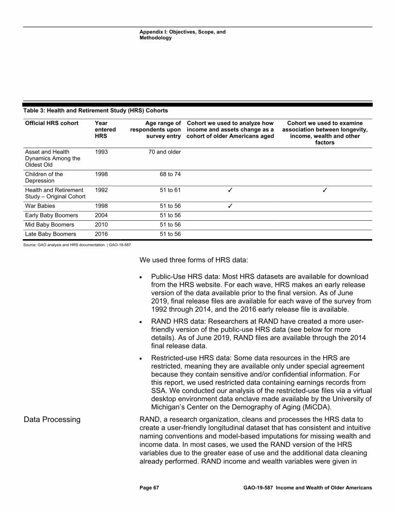
Appendix I: Objectives, Scope, and Methodology
Page 67 GAO-19-587 Income and Wealth of Older Americans
Table 3: Health and Retirement Study (HRS) Cohorts
Official HRS cohort Year entered HRS
Age range of respondents upon
survey entry
Cohort we used to analyze how income and assets change as a cohort of older Americans aged
Cohort we used to examine association between longevity,
income, wealth and other factors
Asset and Health Dynamics Among the Oldest Old
1993 70 and older
Children of the Depression
1998 68 to 74
Health and Retirement Study – Original Cohort
1992 51 to 61 ✓ ✓
War Babies 1998 51 to 56 ✓ Early Baby Boomers 2004 51 to 56 Mid Baby Boomers 2010 51 to 56 Late Baby Boomers 2016 51 to 56
Source: GAO analysis and HRS documentation. | GAO-19-587
We used three forms of HRS data:
• Public-Use HRS data: Most HRS datasets are available for download from the HRS website. For each wave, HRS makes an early release version of the data available prior to the final version. As of June 2019, final release files are available for each wave of the survey from 1992 through 2014, and the 2016 early release file is available.
• RAND HRS data: Researchers at RAND have created a more user-friendly version of the public-use HRS data (see below for more details). As of June 2019, RAND files are available through the 2014 final release data.
• Restricted-use HRS data: Some data resources in the HRS are restricted, meaning they are available only under special agreement because they contain sensitive and/or confidential information. For this report, we used restricted data containing earnings records from SSA. We conducted our analysis of the restricted-use files via a virtual desktop environment data enclave made available by the University of Michigan’s Center on the Demography of Aging (MiCDA).
RAND, a research organization, cleans and processes the HRS data to create a user-friendly longitudinal dataset that has consistent and intuitive naming conventions and model-based imputations for missing wealth and income data. In most cases, we used the RAND version of the HRS variables due to the greater ease of use and the additional data cleaning already performed. RAND income and wealth variables were given in
Data Processing
Appendix I: Objectives, Scope, and Methodology
Page 68 GAO-19-587 Income and Wealth of Older Americans
nominal dollars. We adjusted these variables to real 2016 dollars using the Consumer Price Index for All Urban Consumers. To calculate mortality, we supplemented the RAND files with information from the early release 2016 public use file to the extent that it provided additional information on mortality through 2014. See the data reliability section below for further discussion of the mortality data.
We found the HRS variables presented in this report to be sufficiently reliable. We conducted a data reliability assessment of selected variables by conducting electronic data tests, reviewing documentation on the dataset, and reviewing related internal controls. When we learned that particular variables were not sufficiently reliable, we did not use them in our analysis. We selected our analyses to ensure there was sufficient sample size to produce reliable estimates. We produced variance estimates using a statistical technique chosen to account for the sample design of the HRS and adjusted the sample weights to account for potential bias due to the linkage to SSA administrative data, as described below. We identified additional limitations due to the survey responses being self-reported. As such, they are subject to the respondent’s possible errors in reporting specific financial amounts.
We measured mortality from 1992 through 2014. Mortality data in the HRS, including an indicator for a respondent’s death in a given survey year and month and year of death, come from matches with the National Death Index or follow-up interviews with surviving family members. There is complete date of death (specifically month and year of death) information for nearly everyone who died prior to 2012. However, for deaths since 2012, the HRS data linked to the National Death Index was not available, which likely lead to more deaths without information on month and year of death. Since the 2012 and 2014 survey years, there has been time to gather death date information from follow up interviews with families, and less than 10 percent of those who died between the 2012 and 2014 survey years had incomplete data on month and year of death. However, in the 2016 survey year early release public use file, we found that a higher proportion of those who died did not have death dates, likely due to the lack of linkage with the National Death Index and a lack of time to follow up with families since the 2016 survey year to find out when survey participants died. As a result, we determined that we had reliable data on mortality through 2014.
HRS contains restricted data drawn from SSA administrative sources for participants who have provided explicit consent to link their responses to administrative data and subsequently were successfully linked with the
Data Reliability
Weight Adjustments
Appendix I: Objectives, Scope, and Methodology
Page 69 GAO-19-587 Income and Wealth of Older Americans
administrative data. It is possible that respondents who were linked may differ in systematic ways from respondents who were not linked, which would affect the generalizability of estimates derived solely from the subset of participants who were linked. The survey weights provided with HRS data account for the complexity of the survey design (e.g., oversamples of minorities and Floridians), nonresponse, and post-stratification adjustments for demographic distributions, but do not adjust for the administrative linkage. There is evidence that in at least some waves of the survey, there are modest but statistically significant differences in linkage rates on characteristics including race, income, and wealth.
One technique to address this potential source of bias is to adjust the sample weights used in variance estimation for observed differences between those with and without linked administrative data. Kapteyn et al. suggest a technique for computing inverse probability weights to account for these differences.7 Following this technique, HRS has computed a set of weights that account for consent to SSA administrative linkage, but only for the 1992, 1998, and 2004 survey waves. However, this report needed adjusted household weights for all 12 waves and adjusted respondent weights for wave 1. We opted to address the potential non-linkage bias using a logistic model-based propensity score adjustment, rather than a weighting class adjustment for several reasons. First, we had the benefit of many variables with which to model the propensity of non-linkage. Second, weighting class adjustments, which involve creating mutually exclusive classes based on the variables associated with non-linkage, were not feasible because of the large number of variables we included in the adjustment. The number of respondents per cell would be too small. Third, the propensity score adjustment allows us to consider many variables at the same time. Finally, the propensity score adjustment allows us to rank respondents, rather than assume that the characteristics used in a weighting class adjustment would perfectly predict non-linkage.
We compared estimates and standard errors obtained using the original weights to the non-linkage adjusted weights. The adjusted weights changed estimates and their standard errors in generally small amounts, but did not affect observed trends in this report. For instance, the median absolute value of the change was less than 1 percent for estimates of
7Arie Kapteyn et al., “Effects of Attrition and Non-Response in the Health and Retirement Study,” IZA Discussion Paper Series No. 2246 (August 2006).
Appendix I: Objectives, Scope, and Methodology
Page 70 GAO-19-587 Income and Wealth of Older Americans
median household income for individuals by mid-career earnings quintiles from 1992 to 2014. The median absolute value of the change was 5.7 percent for the standard errors of those estimates.
We used the balanced repeated replication method to estimate standard errors for the income and wealth statistics we reported using HRS because the income and wealth statistics were quantiles (i.e., medians). The standard Taylor series (Woodruff) variance estimation method assumes that quantiles can be expressed as a smooth function in the sample and population. However, quantile functions are not considered smooth. After ruling out Taylor series method, we explored replication methods such as jackknife, bootstrap, and balanced repeated replication. Of those, the balanced repeated replication is most suited for the two primary sampling units per stratum design of the HRS. The Fay adjustment stabilizes the estimates across strata when using the normal balanced repeated replication method. This adjustment is particularly relevant for smaller samples. The literature we reviewed suggested that the jackknife produces a poor estimate of the variance of quantiles (Lohr 2009 and Judkins 1990) and that the bootstrap requires more computations than balanced repeated replication.8
For our analyses, we wanted to classify HRS respondents into income groupings based on a relatively stable measure of income that uses multiple years of administrative data, to reduce measurement error in self-reported survey data and to reduce the chance of basing the income grouping on a single year of unusually low or high income. Several limitations prevent us from classifying households based on their full lifetime income from all sources. HRS does not contain administrative data on income sources besides earnings and Social Security benefits. Moreover, for years before 1978, the administrative earnings records are only available for earnings covered by Social Security and below the taxable maximum. Finally, not all sources of earnings are covered by Social Security. While around 96 percent of employment is currently covered by Social Security, this has not always been the case. In particular, successive expansions of coverage in the 1950s and 1960s greatly increased the proportion of the workforce covered by Social Security, such that relying on SSA earnings records going back to 1951
8Lohr, Sharon L. 2009. Sampling: Design and Analysis. 2nd ed. New York: Brooks/Cole and Judkins, David R. “Fay’s method for variance estimation.” Journal of Official Statistics, vol. 6, no. 3 (1990): 223-239.
Variance Estimation
Mid-Career Household Earnings Measure Construction
Appendix I: Objectives, Scope, and Methodology
Page 71 GAO-19-587 Income and Wealth of Older Americans
would underestimate the earnings of large numbers of older HRS participants.
Thus, for our analysis, we constructed earnings groupings based on a measure of “mid-career” earnings, based on a household’s average annual reported earnings when the household head was age 41 to age 50. Earnings tend to peak (and remain relatively stable) for workers in their mid-40s through their early 50s. We begin measuring earnings at age 41 to avoid using data prior to expansions of Social Security coverage and to minimize our reliance on imputed earnings above the taxable maximum. In the early years of the study, HRS sought retrospective consent for administrative data linkages. As a result, some participants who only provided consent for the administrative linkage during their initial interview and did not provide consent in subsequent interviews did not have earnings records after age 50. Therefore, we set age 50 as the upper bound for our measure of mid-career earnings.
Our goal was to determine how income, wealth, and other demographic and health-related factors are associated with the longevity of older Americans over age 50 in the original HRS cohort. We measured the proportion of original HRS participants still alive at the end of the survey to examine how longevity varied across the income and wealth distributions, as well as across different demographic and health-related variables, including race, educational attainment, gender, and self-reported health status at the beginning of the survey.
Overview
In order to examine these relationships, we used data from the original HRS cohort to measure deaths over a maximum of 22 years (1992 through 2014). Every 2 years, the HRS attempted to measure whether the original respondents were still alive, but these longevity data were incomplete because some of the original respondents declined to
Analyzing the Association Among Income, Wealth, Longevity, and Other Variables
Analysis Goals
Survival Analysis
Appendix I: Objectives, Scope, and Methodology
Page 72 GAO-19-587 Income and Wealth of Older Americans
participate in later waves of the survey. Once these respondents left the survey, their actual longevity could not be followed.9
This incomplete measurement of longevity is generally known as “censored data” in statistics.10 Special methods of “survival analysis” are required to avoid making inaccurate conclusions about actual longevity from this type of data, when the analyst can only measure longevity up to a certain time before death.11 Survival analysis accounts for survey respondents with complete or incomplete longevity data. Without making this distinction, ordinary statistical methods, such as linear regression models of the observed longevities, would not include the correct sample of respondents when estimating the chance that a respondent would die at any time within the observation period. In addition, ordinary methods would incorrectly treat the longevities observed in the observation period as actual longevities, when some of them are the shorter, censored longevities observed before the respondents dropped out of the study. Survival analysis methods correct for this problem, in order to reliably estimate the chance of death by any given time in the observation period.12
9Some of the original respondents continued participating in the survey through 2014, the final year used in our analysis, but had not yet died at the end of the observation period. The HRS could not measure the actual longevity of this second subgroup, because their deaths had not yet occurred. This form of censored data did not affect our analysis, because we do not make inferences about longevity after 2014. Moreover, the end of the observation period was fixed by the release schedule of the HRS public use data files, which should not be systematically related to mortality. 10J.D. Kalbfleisch and R.L. Prentice, The Statistical Analysis of Failure Time Data. New York: John Wiley and Sons, 1980. 39. 11Ibid, 39-41. 12For example, consider a study observes a group of 100 people in 1990, 2000, and 2010. Between 1990 and 2000, 15 people in the group die, and 20 drop out of the study. The likelihood that someone observed in 1990 is still alive in 2000 is 85/100, or 85 percent. Between 2000 and 2010, 10 more people die, and 5 leave the study. There are 65 people still in the study in 2000, so the likelihood that someone observed in 2000 is still alive in 2010 is 55/65, or 84.6 percent. Using only information on the number of people in the group in 1990 who did not die, a simple estimate of the fraction of people who survived until 2010 is (100 - 15 - 10)/100, or 75 percent. However, this estimate does not account for the people who left the study. Using survival analysis to account for people who left the study, the likelihood that someone observed in 1990 is still alive in 2010 is equal to the likelihood that someone lived from 1990 to 2000 and also lived from 2000 to 2010: (85/100)x(55/65), or 71.9 percent. Not accounting for people who leave the study may lead to biased estimates of survival rates.
Appendix I: Objectives, Scope, and Methodology
Page 73 GAO-19-587 Income and Wealth of Older Americans
Most importantly, our analysis assumed actual longevity during the observation period did not have a systematic relationship with whether the original HRS respondents continued to participate in the study except that leaving the study implied a later death (“noninformative censoring”). In other words, participants with censored and actual longevities did not systematically differ in ways that affected longevity or the variables associated with it. We believe this assumption to be reasonable for the purpose of our analysis for two reasons. First, a small percentage (8 percent) of the original respondents dropped out of the survey, so that the impact of any longevity differences among the population who dropped out would likely have been small. Second, while some baseline characteristics of respondents do appear correlated with non-response over time, the population that dropped out of the study does not appear to vary significantly from those completing each wave, except for race and ethnicity.13
Detailed Methods
In our survival analysis, the dependent variable was composed of two parts, including the time in months to death and whether death was observed during the survey period. In general, we used continuous time survival models, including Kaplan-Meier and Cox proportional hazards regression models to estimate survival functions, which estimate the probability of surviving (or dying) up to the end of the survey period, and hazard functions, which estimate the probability of death, per time unit, given that an individual has survived up to that point in time.
We used the Kaplan-Meier method to estimate survival probabilities as a function of time and to obtain univariate statistics on survival for different groups. For example, we estimated the percentage of survivors during the survey period across income and wealth quintiles. We also estimated survivorship across the demographic and health-related variables.
Moreover, using the Cox proportional hazards regression models, we analyzed the relationship between income and longevity and wealth and longevity, controlling for related demographic and health-related variables, as well as age at the beginning of the survey. These regressions allow the relationships between various characteristics and 13Arie Kapteyn, Pierre-Carl Michaud, James Smith, and Arthur van Soest, “Effects of Attrition and Non-Response in the Health and Retirement Study,” IZA Discussion Paper No. 2246 (2006).
Appendix I: Objectives, Scope, and Methodology
Page 74 GAO-19-587 Income and Wealth of Older Americans
death to be described as hazard ratios. For example, hazard ratios that are statistically significant and greater than 1.00 indicate that individuals with those characteristics are more likely to die during the survey period compared to a reference group. Hazard ratios that are statistically significant and less than 1.00 indicate that individuals with those characteristics are less likely to die in the study period compared to a reference group.
We estimated survivorship among individuals with the following characteristics in combination: bottom income (earnings) quintile and no college; middle of the income (earnings) distribution (third quintile) and high school diploma or some college (excluding GED); and top of the income (earnings) distribution and college diploma. We then ran a subset of these scenarios using different combinations of self-reported health status for each of the three main scenarios. For example, we estimated survivorship among individuals in the bottom income (earnings) quintile, who had not attended college, and reported being in fair or poor health in 1992.
Our results have limitations and should be interpreted with caution. Results from the survival analysis present correlations, not causal estimates. Moreover, while our main analysis includes self-reported health status at the beginning of the study period, we also excluded this variable as a sensitivity check given the interconnectedness of income, wealth, and health and the conclusions were similar. Furthermore, due to limitations with respect to the mortality data in later years of the HRS, we did not have specific months and years of death for 60 respondents we know died during the observation period due to death indicators in the interview status variables from HRS. As a result, we imputed their death dates based on the survey year they were indicated to have died in from the HRS interview status questions. While death is continuous in the sense that it can happen to any person at any time, we only observe death within a given month for those with death dates in the data, and only within a year for those whose death information we gathered for the interview status variables. As a sensitivity check, we redid the analysis using survival information at the person-year level and discrete survival analysis techniques and found similar results.
This section describes how we used the HRS to determine how the distributions of income and wealth change as older Americans in the original HRS cohort aged.
Analyzing How Income and Wealth Change as Older Americans Aged
Appendix I: Objectives, Scope, and Methodology
Page 75 GAO-19-587 Income and Wealth of Older Americans
We focused this analysis on the original HRS cohort (born 1931-1941). This cohort entered the study in 1992 at ages 51-61 and had reached their 70s or early 80s by 2014, allowing us to analyze how income and assets changed as these households progressed through retirement.
We conducted our analysis and reported results at the household level because couples may pool financial resources or co-own assets. Also, RAND HRS variables on income and wealth are presented at the household level. When necessary, we combined respondent and spouse or partner level variables we used from the public-use file in order to obtain household-level variables. We restricted this analysis to survey respondents (“household heads”), or any spouses or partners, who were still alive in 2014 to ensure we followed the same group of people throughout our analysis. We grouped households into five earnings groups based on their mid-career earnings, as described above.
Our primary goal was to examine how the distribution of income and wealth changed over time for households in the original HRS cohort, based on their mid-career earnings groups. We also examined how specific sources of income and wealth changed over time. We also wanted to determine how these trends varied based on household demographic characteristics, including race and ethnicity and education level, without attempting to ascribe causality. Our analysis included survey respondents (heads of households) or their spouses or partners who responded to the survey in 1992 and were still alive and responded in 2014, which is the most recent year for which the data are complete. The heads of households we analyzed were from the original HRS cohort and were born in 1931 to 1941. If neither the head of household or the spouse or partner interviewed in 1992 was still alive in 2014, their household was not included in our sample.
In order to do so, we estimated median levels of household wealth and income every 2 years for each earnings group, as well as median levels for specific sources of income and wealth. We estimated the percentage changes and absolute changes in median wealth and income for each earnings group from 1992 through 2014 in order to determine whether income or wealth levels increased or decreased over time. For specific sources of income and wealth, we estimated medians for all households in each earnings group as well as for only those households which reported having the specific source of income or wealth. For example, we determined the median home equity for all households in each earnings group as well as the median home equity for only those households with home equity for each earnings group. Finally, we calculated the percent
Key Definitions and Assumptions
Analysis Goals
Appendix I: Objectives, Scope, and Methodology
Page 76 GAO-19-587 Income and Wealth of Older Americans
of our sample having each type of wealth and income (e.g. home equity, Social Security benefits) for each year in the data. As a sensitivity check, we also analyzed how total assets and income changed for the HRS’s “War Babies” cohort (born 1942-1947). For this analysis, we report 99 percent confidence intervals alongside the percentage or other numerical estimates. We chose to use this level of confidence to account for the use of imputation in the RAND HRS data in addition to the sampling error that using survey data introduces. All financial figures using the HRS data are in 2016 dollars.

Appendix II: Financial and Demographic Characteristics across the Wealth Distribution
Page 77 GAO-19-587 Income and Wealth of Older Americans
This appendix compares the top 1 percent of the wealth distribution of older households to several other groups in this distribution: (1) the next 19 percent, (2) the top 20 percent, (3) the bottom 80 percent, and (4) the bottom 20 percent. These comparisons provide context for the financial security of the top 1 percent relative to other households at the top of the wealth distribution, the remainder of the wealth distribution, and households at the bottom of the distribution, respectively.
To draw these comparisons, we used 2016 data from the Survey of Consumer Finances, a triennial, cross-sectional survey produced by the Board of Governors of the Federal Reserve System. A different sample of households was used for each year in our analysis. These data allow for comparison of the experiences of same-age households at different points in time. We chose to look at household-level resources because couples may pool their economic resources, and the SCF asks some of its questions about resources for households. We conducted our analysis for older households, which were defined as those in which the household head or any spouse or partner were ages 55 or older. We defined wealth as net worth, or assets minus debt. Because the sample size for the top 1 percent is small, we presented dollar values rounded to thousands of 2016 dollars.
Appendix II: Financial and Demographic Characteristics across the Wealth Distribution
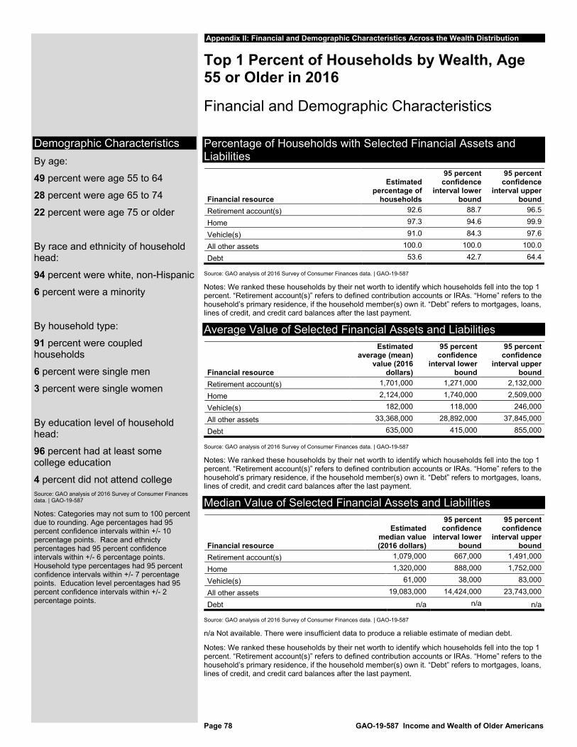
Page 78 GAO-19-587 Income and Wealth of Older Americans
Appendix II: Financial and Demographic Characteristics Across the Wealth Distribution
Top 1 Percent of Households by Wealth, Age 55 or Older in 2016
Financial and Demographic Characteristics
Percentage of Households with Selected Financial Assets and Liabilities
Financial resource
Estimated percentage of
households
95 percent confidence
interval lower bound
95 percent confidence
interval upper bound
Retirement account(s) 92.6 88.7 96.5
Home 97.3 94.6 99.9
Vehicle(s) 91.0 84.3 97.6
All other assets 100.0 100.0 100.0
Debt 53.6 42.7 64.4
Source: GAO analysis of 2016 Survey of Consumer Finances data. | GAO-19-587
Notes: We ranked these households by their net worth to identify which households fell into the top 1 percent. “Retirement account(s)” refers to defined contribution accounts or IRAs. “Home” refers to the household’s primary residence, if the household member(s) own it. “Debt” refers to mortgages, loans, lines of credit, and credit card balances after the last payment.
Average Value of Selected Financial Assets and Liabilities
Financial resource
Estimated average (mean)
value (2016 dollars)
95 percent confidence
interval lower bound
95 percent confidence
interval upper bound
Retirement account(s) 1,701,000 1,271,000 2,132,000
Home 2,124,000 1,740,000 2,509,000
Vehicle(s) 182,000 118,000 246,000
All other assets 33,368,000 28,892,000 37,845,000
Debt 635,000 415,000 855,000
Source: GAO analysis of 2016 Survey of Consumer Finances data. | GAO-19-587
Notes: We ranked these households by their net worth to identify which households fell into the top 1 percent. “Retirement account(s)” refers to defined contribution accounts or IRAs. “Home” refers to the household’s primary residence, if the household member(s) own it. “Debt” refers to mortgages, loans, lines of credit, and credit card balances after the last payment.
Median Value of Selected Financial Assets and Liabilities
Financial resource
Estimated median value (2016 dollars)
95 percent confidence
interval lower bound
95 percent confidence
interval upper bound
Retirement account(s) 1,079,000 667,000 1,491,000
Home 1,320,000 888,000 1,752,000
Vehicle(s) 61,000 38,000 83,000
All other assets 19,083,000 14,424,000 23,743,000
Debt n/a n/a n/a
Source: GAO analysis of 2016 Survey of Consumer Finances data. | GAO-19-587
n/a Not available. There were insufficient data to produce a reliable estimate of median debt.
Notes: We ranked these households by their net worth to identify which households fell into the top 1 percent. “Retirement account(s)” refers to defined contribution accounts or IRAs. “Home” refers to the household’s primary residence, if the household member(s) own it. “Debt” refers to mortgages, loans, lines of credit, and credit card balances after the last payment.
Demographic Characteristics By age:
49 percent were age 55 to 64
28 percent were age 65 to 74
22 percent were age 75 or older
By race and ethnicity of household head:
94 percent were white, non-Hispanic
6 percent were a minority
By household type:
91 percent were coupled households
6 percent were single men
3 percent were single women
By education level of household head:
96 percent had at least some college education
4 percent did not attend college Source: GAO analysis of 2016 Survey of Consumer Finances data. | GAO-19-587
Notes: Categories may not sum to 100 percent due to rounding. Age percentages had 95 percent confidence intervals within +/- 10 percentage points. Race and ethnicty percentages had 95 percent confidence intervals within +/- 6 percentage points. Household type percentages had 95 percent confidence intervals within +/- 7 percentage points. Education level percentages had 95 percent confidence intervals within +/- 2 percentage points.
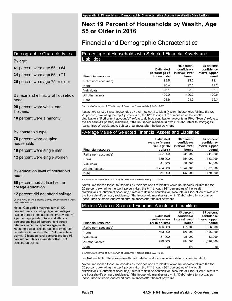
Page 79 GAO-19-587 Income and Wealth of Older Americans
Appendix II: Financial and Demographic Characteristics Across the Wealth Distribution
Next 19 Percent of Households by Wealth, Age 55 or Older in 2016
Financial and Demographic Characteristics
Percentage of Households with Selected Financial Assets and Liabilities
Financial resource
Estimated percentage of
households
95 percent confidence
interval lower bound
95 percent confidence
interval upper bound
Retirement account(s) 85.5 83.0 88.1
Home 95.4 93.5 97.2
Vehicle(s) 95.1 93.6 96.7
All other assets 100.0 100.0 100.0
Debt 64.8 61.3 68.3
Source: GAO analysis of 2016 Survey of Consumer Finances data. | GAO-19-587
Notes: We ranked these households by their net worth to identify which households fell into the top 20 percent, excluding the top 1 percent (i.e., the 81st through 99th percentiles of the wealth distribution). “Retirement account(s)” refers to defined contribution accounts or IRAs. “Home” refers to the household’s primary residence, if the household member(s) own it. “Debt” refers to mortgages, loans, lines of credit, and credit card balances after the last payment.
Average Value of Selected Financial Assets and Liabilities
Financial resource
Estimated average (mean)
value (2016 dollars)
95 percent confidence
interval lower bound
95 percent confidence
interval upper bound
Retirement account(s) 687,000 634,000 741,000
Home 589,000 554,000 623,000
Vehicle(s) 41,000 38,000 44,000
All other assets 1,754,000 1,642,000 1,867,000
Debt 151,000 132,000 170,000
Source: GAO analysis of 2016 Survey of Consumer Finances data. | GAO-19-587
Notes: We ranked these households by their net worth to identify which households fell into the top 20 percent, excluding the top 1 percent (i.e., the 81st through 99th percentiles of the wealth distribution). “Retirement account(s)” refers to defined contribution accounts or IRAs. “Home” refers to the household’s primary residence, if the household member(s) own it. “Debt” refers to mortgages, loans, lines of credit, and credit card balances after the last payment.
Median Value of Selected Financial Assets and Liabilities
Financial resource
Estimated median value (2016 dollars)
95 percent confidence
interval lower bound
95 percent confidence
interval upper bound
Retirement account(s) 486,000 415,000 556,000
Home 463,000 420,000 506,000
Vehicle(s) 31,000 28,000 33,000
All other assets 990,000 884,000 1,096,000
Debt n/a n/a n/a
Source: GAO analysis of 2016 Survey of Consumer Finances data. | GAO-19-587
n/a Not available. There were insufficient data to produce a reliable estimate of median debt.
Notes: We ranked these households by their net worth to identify which households fell into the top 20 percent, excluding the top 1 percent (i.e., the 81st through 99th percentiles of the wealth distribution). “Retirement account(s)” refers to defined contribution accounts or IRAs. “Home” refers to the household’s primary residence, if the household member(s) own it. “Debt” refers to mortgages, loans, lines of credit, and credit card balances after the last payment.
Demographic Characteristics By age:
41 percent were age 55 to 64
34 percent were age 65 to 74
26 percent were age 75 or older
By race and ethnicity of household head:
90 percent were white, non-Hispanic
10 percent were a minority
By household type:
78 percent were coupled households
10 percent were single men
12 percent were single women
By education level of household head:
88 percent had at least some college education
12 percent did not attend college Source: GAO analysis of 2016 Survey of Consumer Finances data.| GAO-19-587
Notes: Categories may not sum to 100 percent due to rounding. Age percentages had 95 percent confidence intervals within +/- 4 percentage points. Race and ethnicty percentages had 95 percent confidence intervals within +/- 3 percentage points. Household type percentages had 95 percent confidence intervals within +/- 4 percentage points. Education level percentages had 95 percent confidence intervals within +/- 3 percentage points.
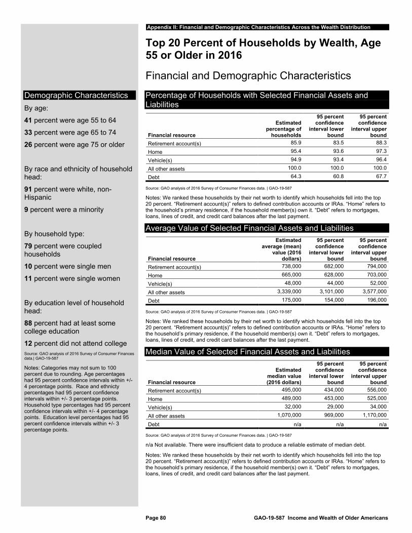
Page 80 GAO-19-587 Income and Wealth of Older Americans
Appendix II: Financial and Demographic Characteristics Across the Wealth Distribution
Top 20 Percent of Households by Wealth, Age 55 or Older in 2016
Financial and Demographic Characteristics
Percentage of Households with Selected Financial Assets and Liabilities
Financial resource
Estimated percentage of
households
95 percent confidence
interval lower bound
95 percent confidence
interval upper bound
Retirement account(s) 85.9 83.5 88.3
Home 95.4 93.6 97.3
Vehicle(s) 94.9 93.4 96.4
All other assets 100.0 100.0 100.0
Debt 64.3 60.8 67.7
Source: GAO analysis of 2016 Survey of Consumer Finances data. | GAO-19-587
Notes: We ranked these households by their net worth to identify which households fell into the top 20 percent. “Retirement account(s)” refers to defined contribution accounts or IRAs. “Home” refers to the household’s primary residence, if the household member(s) own it. “Debt” refers to mortgages, loans, lines of credit, and credit card balances after the last payment.
Average Value of Selected Financial Assets and Liabilities
Financial resource
Estimated average (mean)
value (2016 dollars)
95 percent confidence
interval lower bound
95 percent confidence
interval upper bound
Retirement account(s) 738,000 682,000 794,000
Home 665,000 628,000 703,000
Vehicle(s) 48,000 44,000 52,000
All other assets 3,339,000 3,101,000 3,577,000
Debt 175,000 154,000 196,000
Source: GAO analysis of 2016 Survey of Consumer Finances data. | GAO-19-587
Notes: We ranked these households by their net worth to identify which households fell into the top 20 percent. “Retirement account(s)” refers to defined contribution accounts or IRAs. “Home” refers to the household’s primary residence, if the household member(s) own it. “Debt” refers to mortgages, loans, lines of credit, and credit card balances after the last payment.
Median Value of Selected Financial Assets and Liabilities
Financial resource
Estimated median value (2016 dollars)
95 percent confidence
interval lower bound
95 percent confidence
interval upper bound
Retirement account(s) 495,000 434,000 556,000
Home 489,000 453,000 525,000
Vehicle(s) 32,000 29,000 34,000
All other assets 1,070,000 969,000 1,170,000
Debt n/a n/a n/a
Source: GAO analysis of 2016 Survey of Consumer Finances data. | GAO-19-587
n/a Not available. There were insufficient data to produce a reliable estimate of median debt.
Notes: We ranked these households by their net worth to identify which households fell into the top 20 percent. “Retirement account(s)” refers to defined contribution accounts or IRAs. “Home” refers to the household’s primary residence, if the household member(s) own it. “Debt” refers to mortgages, loans, lines of credit, and credit card balances after the last payment.
Demographic Characteristics By age:
41 percent were age 55 to 64
33 percent were age 65 to 74
26 percent were age 75 or older
By race and ethnicity of household head:
91 percent were white, non-Hispanic
9 percent were a minority
By household type:
79 percent were coupled households
10 percent were single men
11 percent were single women
By education level of household head:
88 percent had at least some college education
12 percent did not attend college Source: GAO analysis of 2016 Survey of Consumer Finances data.| GAO-19-587
Notes: Categories may not sum to 100 percent due to rounding. Age percentages had 95 percent confidence intervals within +/- 4 percentage points. Race and ethnicty percentages had 95 percent confidence intervals within +/- 3 percentage points. Household type percentages had 95 percent confidence intervals within +/- 4 percentage points. Education level percentages had 95 percent confidence intervals within +/- 3 percentage points.
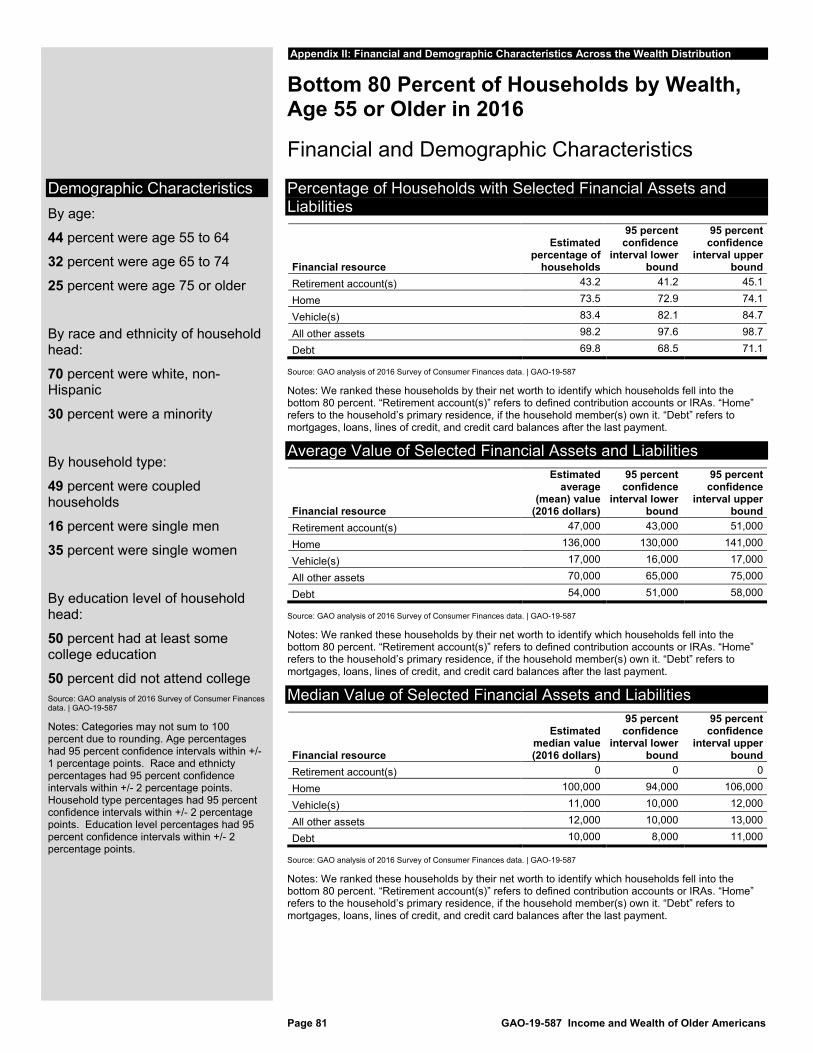
Page 81 GAO-19-587 Income and Wealth of Older Americans
Appendix II: Financial and Demographic Characteristics Across the Wealth Distribution
Bottom 80 Percent of Households by Wealth, Age 55 or Older in 2016
Financial and Demographic Characteristics
Percentage of Households with Selected Financial Assets and Liabilities
Financial resource
Estimated percentage of
households
95 percent confidence
interval lower bound
95 percent confidence
interval upper bound
Retirement account(s) 43.2 41.2 45.1
Home 73.5 72.9 74.1
Vehicle(s) 83.4 82.1 84.7
All other assets 98.2 97.6 98.7
Debt 69.8 68.5 71.1
Source: GAO analysis of 2016 Survey of Consumer Finances data. | GAO-19-587
Notes: We ranked these households by their net worth to identify which households fell into the bottom 80 percent. “Retirement account(s)” refers to defined contribution accounts or IRAs. “Home” refers to the household’s primary residence, if the household member(s) own it. “Debt” refers to mortgages, loans, lines of credit, and credit card balances after the last payment.
Average Value of Selected Financial Assets and Liabilities
Financial resource
Estimated average
(mean) value (2016 dollars)
95 percent confidence
interval lower bound
95 percent confidence
interval upper bound
Retirement account(s) 47,000 43,000 51,000
Home 136,000 130,000 141,000
Vehicle(s) 17,000 16,000 17,000
All other assets 70,000 65,000 75,000
Debt 54,000 51,000 58,000
Source: GAO analysis of 2016 Survey of Consumer Finances data. | GAO-19-587
Notes: We ranked these households by their net worth to identify which households fell into the bottom 80 percent. “Retirement account(s)” refers to defined contribution accounts or IRAs. “Home” refers to the household’s primary residence, if the household member(s) own it. “Debt” refers to mortgages, loans, lines of credit, and credit card balances after the last payment.
Median Value of Selected Financial Assets and Liabilities
Financial resource
Estimated median value (2016 dollars)
95 percent confidence
interval lower bound
95 percent confidence
interval upper bound
Retirement account(s) 0 0 0
Home 100,000 94,000 106,000
Vehicle(s) 11,000 10,000 12,000
All other assets 12,000 10,000 13,000
Debt 10,000 8,000 11,000
Source: GAO analysis of 2016 Survey of Consumer Finances data. | GAO-19-587
Notes: We ranked these households by their net worth to identify which households fell into the bottom 80 percent. “Retirement account(s)” refers to defined contribution accounts or IRAs. “Home” refers to the household’s primary residence, if the household member(s) own it. “Debt” refers to mortgages, loans, lines of credit, and credit card balances after the last payment.
Demographic Characteristics By age:
44 percent were age 55 to 64
32 percent were age 65 to 74
25 percent were age 75 or older
By race and ethnicity of household head:
70 percent were white, non-Hispanic
30 percent were a minority
By household type:
49 percent were coupled households
16 percent were single men
35 percent were single women
By education level of household head:
50 percent had at least some college education 50 percent did not attend college Source: GAO analysis of 2016 Survey of Consumer Finances data. | GAO-19-587
Notes: Categories may not sum to 100 percent due to rounding. Age percentages had 95 percent confidence intervals within +/- 1 percentage points. Race and ethnicty percentages had 95 percent confidence intervals within +/- 2 percentage points. Household type percentages had 95 percent confidence intervals within +/- 2 percentage points. Education level percentages had 95 percent confidence intervals within +/- 2 percentage points.
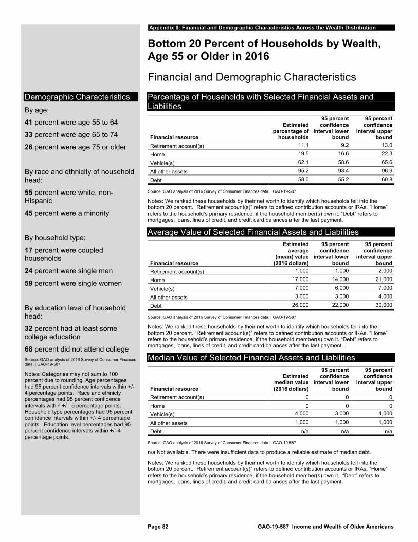
Page 82 GAO-19-587 Income and Wealth of Older Americans
Appendix II: Financial and Demographic Characteristics Across the Wealth Distribution
Bottom 20 Percent of Households by Wealth, Age 55 or Older in 2016
Financial and Demographic Characteristics
Percentage of Households with Selected Financial Assets and Liabilities
Financial resource
Estimated percentage of
households
95 percent confidence
interval lower bound
95 percent confidence
interval upper bound
Retirement account(s) 11.1 9.2 13.0
Home 19.5 16.6 22.3
Vehicle(s) 62.1 58.6 65.6
All other assets 95.2 93.4 96.9
Debt 58.0 55.2 60.8
Source: GAO analysis of 2016 Survey of Consumer Finances data. | GAO-19-587
Notes: We ranked these households by their net worth to identify which households fell into the bottom 20 percent. “Retirement account(s)” refers to defined contribution accounts or IRAs. “Home” refers to the household’s primary residence, if the household member(s) own it. “Debt” refers to mortgages, loans, lines of credit, and credit card balances after the last payment.
Average Value of Selected Financial Assets and Liabilities
Financial resource
Estimated average
(mean) value (2016 dollars)
95 percent confidence
interval lower bound
95 percent confidence
interval upper bound
Retirement account(s) 1,000 1,000 2,000
Home 17,000 14,000 21,000
Vehicle(s) 7,000 6,000 7,000
All other assets 3,000 3,000 4,000
Debt 26,000 22,000 30,000
Source: GAO analysis of 2016 Survey of Consumer Finances data. | GAO-19-587
Notes: We ranked these households by their net worth to identify which households fell into the bottom 20 percent. “Retirement account(s)” refers to defined contribution accounts or IRAs. “Home” refers to the household’s primary residence, if the household member(s) own it. “Debt” refers to mortgages, loans, lines of credit, and credit card balances after the last payment.
Median Value of Selected Financial Assets and Liabilities
Financial resource
Estimated median value (2016 dollars)
95 percent confidence
interval lower bound
95 percent confidence
interval upper bound
Retirement account(s) 0 0 0 Home 0 0 0 Vehicle(s) 4,000 3,000 4,000
All other assets 1,000 1,000 1,000
Debt n/a n/a n/a
Source: GAO analysis of 2016 Survey of Consumer Finances data. | GAO-19-587
n/a Not available. There were insufficient data to produce a reliable estimate of median debt.
Notes: We ranked these households by their net worth to identify which households fell into the bottom 20 percent. “Retirement account(s)” refers to defined contribution accounts or IRAs. “Home” refers to the household’s primary residence, if the household member(s) own it. “Debt” refers to mortgages, loans, lines of credit, and credit card balances after the last payment.
Demographic Characteristics By age:
41 percent were age 55 to 64
33 percent were age 65 to 74
26 percent were age 75 or older
By race and ethnicity of household head:
55 percent were white, non-Hispanic
45 percent were a minority
By household type:
17 percent were coupled households
24 percent were single men
59 percent were single women
By education level of household head:
32 percent had at least some college education 68 percent did not attend college Source: GAO analysis of 2016 Survey of Consumer Finances data. | GAO-19-587
Notes: Categories may not sum to 100 percent due to rounding. Age percentages had 95 percent confidence intervals within +/- 4 percentage points. Race and ethnicty percentages had 95 percent confidence intervals within +/- 5 percentage points. Household type percentages had 95 percent confidence intervals within +/- 4 percentage points. Education level percentages had 95 percent confidence intervals within +/- 4 percentage points.
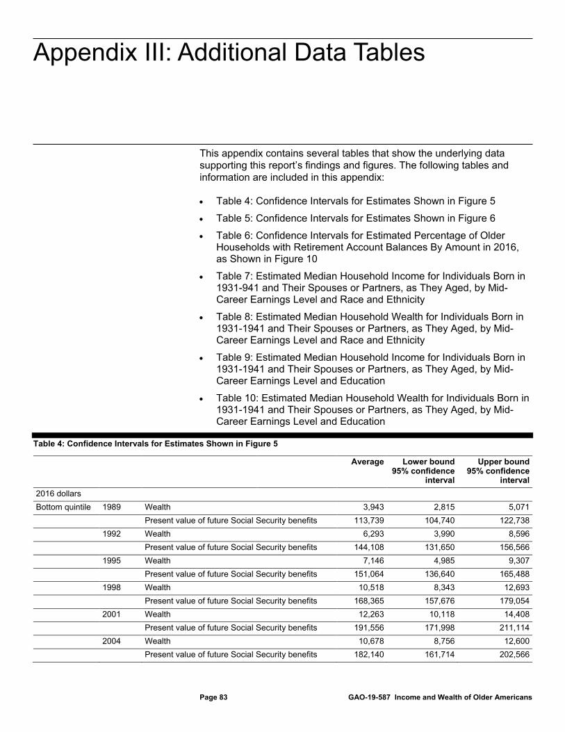
Appendix III: Additional Data Tables
Page 83 GAO-19-587 Income and Wealth of Older Americans
This appendix contains several tables that show the underlying data supporting this report’s findings and figures. The following tables and information are included in this appendix:
• Table 4: Confidence Intervals for Estimates Shown in Figure 5
• Table 5: Confidence Intervals for Estimates Shown in Figure 6
• Table 6: Confidence Intervals for Estimated Percentage of Older Households with Retirement Account Balances By Amount in 2016, as Shown in Figure 10
• Table 7: Estimated Median Household Income for Individuals Born in 1931-941 and Their Spouses or Partners, as They Aged, by Mid-Career Earnings Level and Race and Ethnicity
• Table 8: Estimated Median Household Wealth for Individuals Born in 1931-1941 and Their Spouses or Partners, as They Aged, by Mid-Career Earnings Level and Race and Ethnicity
• Table 9: Estimated Median Household Income for Individuals Born in 1931-1941 and Their Spouses or Partners, as They Aged, by Mid-Career Earnings Level and Education
• Table 10: Estimated Median Household Wealth for Individuals Born in 1931-1941 and Their Spouses or Partners, as They Aged, by Mid-Career Earnings Level and Education
Table 4: Confidence Intervals for Estimates Shown in Figure 5
Average Lower bound 95% confidence
interval
Upper bound 95% confidence
interval 2016 dollars Bottom quintile 1989 Wealth 3,943 2,815 5,071 Present value of future Social Security benefits 113,739 104,740 122,738 1992 Wealth 6,293 3,990 8,596 Present value of future Social Security benefits 144,108 131,650 156,566 1995 Wealth 7,146 4,985 9,307 Present value of future Social Security benefits 151,064 136,640 165,488 1998 Wealth 10,518 8,343 12,693 Present value of future Social Security benefits 168,365 157,676 179,054 2001 Wealth 12,263 10,118 14,408 Present value of future Social Security benefits 191,556 171,998 211,114 2004 Wealth 10,678 8,756 12,600 Present value of future Social Security benefits 182,140 161,714 202,566
Appendix III: Additional Data Tables
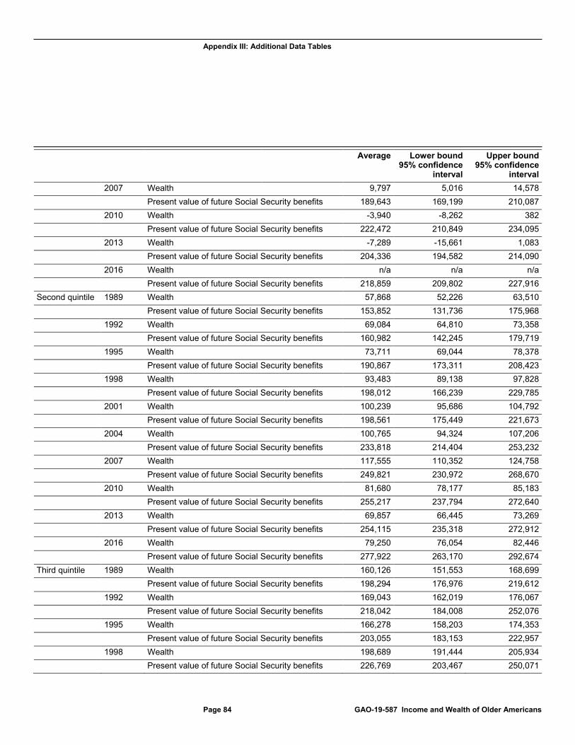
Appendix III: Additional Data Tables
Page 84 GAO-19-587 Income and Wealth of Older Americans
Average Lower bound 95% confidence
interval
Upper bound 95% confidence
interval 2007 Wealth 9,797 5,016 14,578 Present value of future Social Security benefits 189,643 169,199 210,087 2010 Wealth -3,940 -8,262 382 Present value of future Social Security benefits 222,472 210,849 234,095 2013 Wealth -7,289 -15,661 1,083 Present value of future Social Security benefits 204,336 194,582 214,090 2016 Wealth n/a n/a n/a Present value of future Social Security benefits 218,859 209,802 227,916 Second quintile 1989 Wealth 57,868 52,226 63,510 Present value of future Social Security benefits 153,852 131,736 175,968 1992 Wealth 69,084 64,810 73,358 Present value of future Social Security benefits 160,982 142,245 179,719 1995 Wealth 73,711 69,044 78,378 Present value of future Social Security benefits 190,867 173,311 208,423 1998 Wealth 93,483 89,138 97,828 Present value of future Social Security benefits 198,012 166,239 229,785 2001 Wealth 100,239 95,686 104,792 Present value of future Social Security benefits 198,561 175,449 221,673 2004 Wealth 100,765 94,324 107,206 Present value of future Social Security benefits 233,818 214,404 253,232 2007 Wealth 117,555 110,352 124,758 Present value of future Social Security benefits 249,821 230,972 268,670 2010 Wealth 81,680 78,177 85,183 Present value of future Social Security benefits 255,217 237,794 272,640 2013 Wealth 69,857 66,445 73,269 Present value of future Social Security benefits 254,115 235,318 272,912 2016 Wealth 79,250 76,054 82,446 Present value of future Social Security benefits 277,922 263,170 292,674 Third quintile 1989 Wealth 160,126 151,553 168,699 Present value of future Social Security benefits 198,294 176,976 219,612 1992 Wealth 169,043 162,019 176,067 Present value of future Social Security benefits 218,042 184,008 252,076 1995 Wealth 166,278 158,203 174,353 Present value of future Social Security benefits 203,055 183,153 222,957 1998 Wealth 198,689 191,444 205,934 Present value of future Social Security benefits 226,769 203,467 250,071
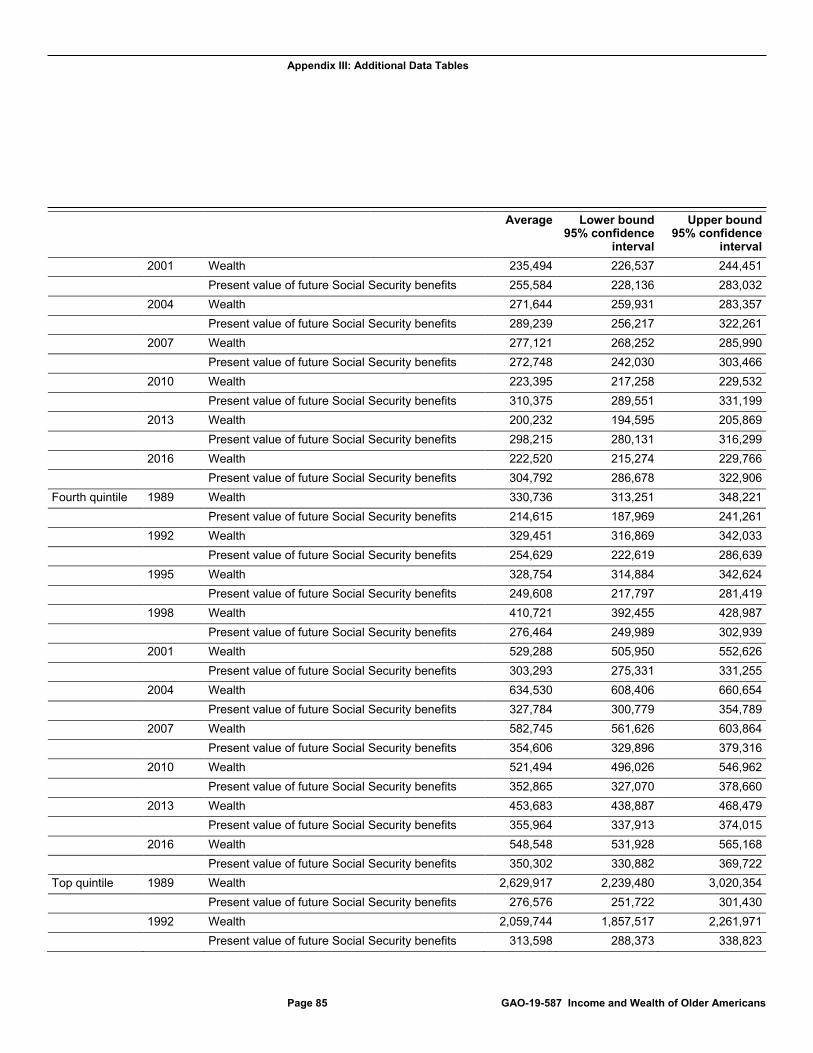
Appendix III: Additional Data Tables
Page 85 GAO-19-587 Income and Wealth of Older Americans
Average Lower bound 95% confidence
interval
Upper bound 95% confidence
interval 2001 Wealth 235,494 226,537 244,451 Present value of future Social Security benefits 255,584 228,136 283,032 2004 Wealth 271,644 259,931 283,357 Present value of future Social Security benefits 289,239 256,217 322,261 2007 Wealth 277,121 268,252 285,990 Present value of future Social Security benefits 272,748 242,030 303,466 2010 Wealth 223,395 217,258 229,532 Present value of future Social Security benefits 310,375 289,551 331,199 2013 Wealth 200,232 194,595 205,869 Present value of future Social Security benefits 298,215 280,131 316,299 2016 Wealth 222,520 215,274 229,766 Present value of future Social Security benefits 304,792 286,678 322,906 Fourth quintile 1989 Wealth 330,736 313,251 348,221 Present value of future Social Security benefits 214,615 187,969 241,261 1992 Wealth 329,451 316,869 342,033 Present value of future Social Security benefits 254,629 222,619 286,639 1995 Wealth 328,754 314,884 342,624 Present value of future Social Security benefits 249,608 217,797 281,419 1998 Wealth 410,721 392,455 428,987 Present value of future Social Security benefits 276,464 249,989 302,939 2001 Wealth 529,288 505,950 552,626 Present value of future Social Security benefits 303,293 275,331 331,255 2004 Wealth 634,530 608,406 660,654 Present value of future Social Security benefits 327,784 300,779 354,789 2007 Wealth 582,745 561,626 603,864 Present value of future Social Security benefits 354,606 329,896 379,316 2010 Wealth 521,494 496,026 546,962 Present value of future Social Security benefits 352,865 327,070 378,660 2013 Wealth 453,683 438,887 468,479 Present value of future Social Security benefits 355,964 337,913 374,015 2016 Wealth 548,548 531,928 565,168 Present value of future Social Security benefits 350,302 330,882 369,722 Top quintile 1989 Wealth 2,629,917 2,239,480 3,020,354 Present value of future Social Security benefits 276,576 251,722 301,430 1992 Wealth 2,059,744 1,857,517 2,261,971 Present value of future Social Security benefits 313,598 288,373 338,823
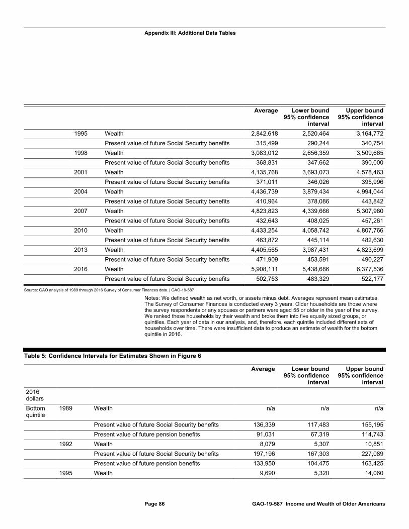
Appendix III: Additional Data Tables
Page 86 GAO-19-587 Income and Wealth of Older Americans
Average Lower bound 95% confidence
interval
Upper bound 95% confidence
interval 1995 Wealth 2,842,618 2,520,464 3,164,772 Present value of future Social Security benefits 315,499 290,244 340,754 1998 Wealth 3,083,012 2,656,359 3,509,665 Present value of future Social Security benefits 368,831 347,662 390,000 2001 Wealth 4,135,768 3,693,073 4,578,463 Present value of future Social Security benefits 371,011 346,026 395,996 2004 Wealth 4,436,739 3,879,434 4,994,044 Present value of future Social Security benefits 410,964 378,086 443,842 2007 Wealth 4,823,823 4,339,666 5,307,980 Present value of future Social Security benefits 432,643 408,025 457,261 2010 Wealth 4,433,254 4,058,742 4,807,766 Present value of future Social Security benefits 463,872 445,114 482,630 2013 Wealth 4,405,565 3,987,431 4,823,699 Present value of future Social Security benefits 471,909 453,591 490,227 2016 Wealth 5,908,111 5,438,686 6,377,536 Present value of future Social Security benefits 502,753 483,329 522,177
Source: GAO analysis of 1989 through 2016 Survey of Consumer Finances data. | GAO-19-587
Notes: We defined wealth as net worth, or assets minus debt. Averages represent mean estimates. The Survey of Consumer Finances is conducted every 3 years. Older households are those where the survey respondents or any spouses or partners were aged 55 or older in the year of the survey. We ranked these households by their wealth and broke them into five equally sized groups, or quintiles. Each year of data in our analysis, and, therefore, each quintile included different sets of households over time. There were insufficient data to produce an estimate of wealth for the bottom quintile in 2016.
Table 5: Confidence Intervals for Estimates Shown in Figure 6
Average Lower bound 95% confidence
interval
Upper bound 95% confidence
interval 2016 dollars
Bottom quintile
1989 Wealth n/a n/a n/a
Present value of future Social Security benefits 136,339 117,483 155,195 Present value of future pension benefits 91,031 67,319 114,743 1992 Wealth 8,079 5,307 10,851 Present value of future Social Security benefits 197,196 167,303 227,089 Present value of future pension benefits 133,950 104,475 163,425 1995 Wealth 9,690 5,320 14,060
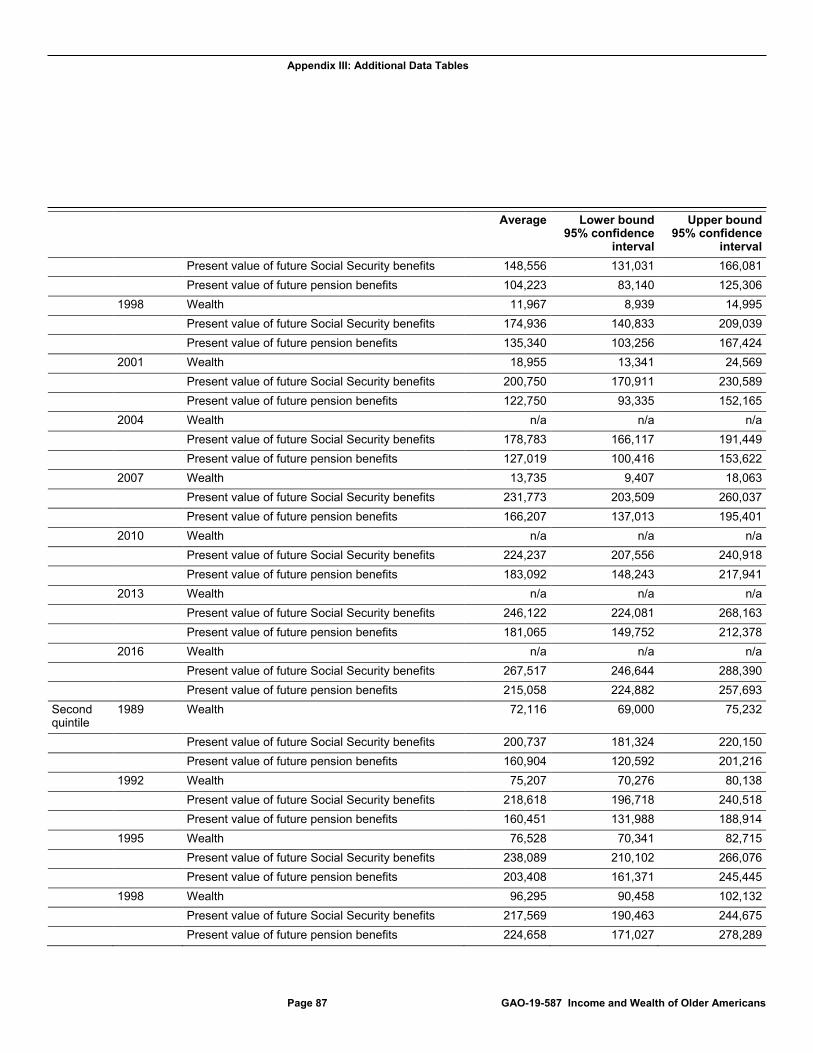
Appendix III: Additional Data Tables
Page 87 GAO-19-587 Income and Wealth of Older Americans
Average Lower bound 95% confidence
interval
Upper bound 95% confidence
interval Present value of future Social Security benefits 148,556 131,031 166,081 Present value of future pension benefits 104,223 83,140 125,306 1998 Wealth 11,967 8,939 14,995 Present value of future Social Security benefits 174,936 140,833 209,039 Present value of future pension benefits 135,340 103,256 167,424 2001 Wealth 18,955 13,341 24,569 Present value of future Social Security benefits 200,750 170,911 230,589 Present value of future pension benefits 122,750 93,335 152,165 2004 Wealth n/a n/a n/a Present value of future Social Security benefits 178,783 166,117 191,449 Present value of future pension benefits 127,019 100,416 153,622 2007 Wealth 13,735 9,407 18,063 Present value of future Social Security benefits 231,773 203,509 260,037 Present value of future pension benefits 166,207 137,013 195,401 2010 Wealth n/a n/a n/a Present value of future Social Security benefits 224,237 207,556 240,918 Present value of future pension benefits 183,092 148,243 217,941 2013 Wealth n/a n/a n/a Present value of future Social Security benefits 246,122 224,081 268,163 Present value of future pension benefits 181,065 149,752 212,378 2016 Wealth n/a n/a n/a Present value of future Social Security benefits 267,517 246,644 288,390 Present value of future pension benefits 215,058 224,882 257,693 Second quintile
1989 Wealth 72,116 69,000 75,232
Present value of future Social Security benefits 200,737 181,324 220,150 Present value of future pension benefits 160,904 120,592 201,216 1992 Wealth 75,207 70,276 80,138 Present value of future Social Security benefits 218,618 196,718 240,518 Present value of future pension benefits 160,451 131,988 188,914 1995 Wealth 76,528 70,341 82,715 Present value of future Social Security benefits 238,089 210,102 266,076 Present value of future pension benefits 203,408 161,371 245,445 1998 Wealth 96,295 90,458 102,132 Present value of future Social Security benefits 217,569 190,463 244,675 Present value of future pension benefits 224,658 171,027 278,289
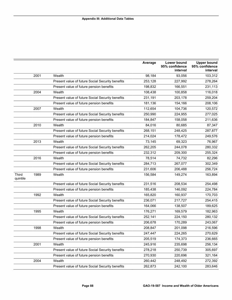
Appendix III: Additional Data Tables
Page 88 GAO-19-587 Income and Wealth of Older Americans
Average Lower bound 95% confidence
interval
Upper bound 95% confidence
interval 2001 Wealth 98,184 93,056 103,312 Present value of future Social Security benefits 253,128 227,992 278,264 Present value of future pension benefits 198,832 166,551 231,113 2004 Wealth 108,438 100,858 116,018 Present value of future Social Security benefits 231,191 203,178 259,204 Present value of future pension benefits 181,136 154,166 208,106 2007 Wealth 112,654 104,736 120,572 Present value of future Social Security benefits 250,990 224,955 277,025 Present value of future pension benefits 184,847 158,058 211,636 2010 Wealth 84,016 80,685 87,347 Present value of future Social Security benefits 268,151 248,425 287,877 Present value of future pension benefits 214,024 178,472 249,576 2013 Wealth 73,145 69,323 76,967 Present value of future Social Security benefits 262,205 244,078 280,332 Present value of future pension benefits 232,312 209,300 255,324 2016 Wealth 78,514 74,732 82,296 Present value of future Social Security benefits 284,713 267,077 302,349 Present value of future pension benefits 231,606 206,488 256,724 Third quintile
1989 Wealth 156,584 149,274 163,894
Present value of future Social Security benefits 231,516 208,534 254,498 Present value of future pension benefits 185,438 146,092 224,784 1992 Wealth 165,820 160,937 170,703 Present value of future Social Security benefits 236,071 217,727 254,415 Present value of future pension benefits 164,066 138,507 189,625 1995 Wealth 176,271 169,579 182,963 Present value of future Social Security benefits 252,141 224,150 280,132 Present value of future pension benefits 206,678 170,289 243,067 1998 Wealth 208,847 201,098 216,596 Present value of future Social Security benefits 247,447 224,265 270,629 Present value of future pension benefits 205,519 174,373 236,665 2001 Wealth 245,916 235,698 256,134 Present value of future Social Security benefits 278,218 250,739 305,697 Present value of future pension benefits 270,930 220,696 321,164 2004 Wealth 260,442 248,492 272,392 Present value of future Social Security benefits 262,873 242,100 283,646
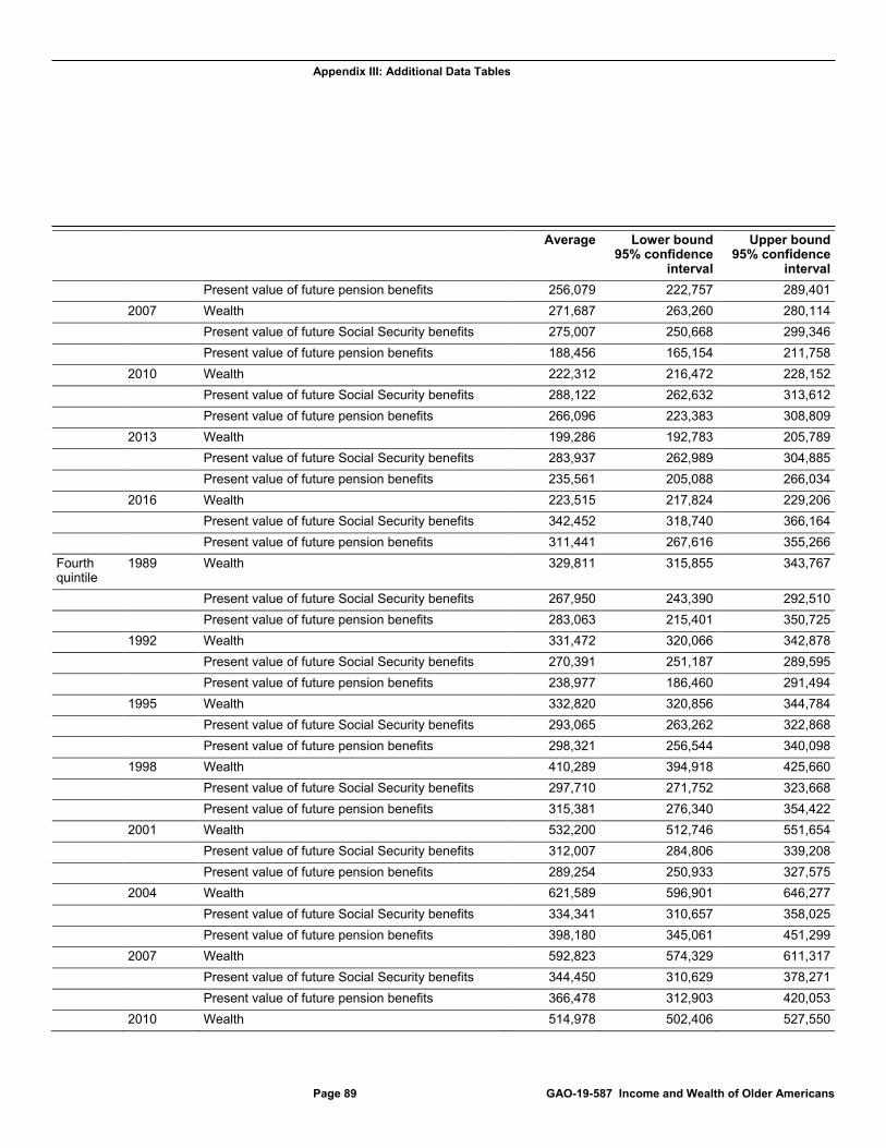
Appendix III: Additional Data Tables
Page 89 GAO-19-587 Income and Wealth of Older Americans
Average Lower bound 95% confidence
interval
Upper bound 95% confidence
interval Present value of future pension benefits 256,079 222,757 289,401 2007 Wealth 271,687 263,260 280,114 Present value of future Social Security benefits 275,007 250,668 299,346 Present value of future pension benefits 188,456 165,154 211,758 2010 Wealth 222,312 216,472 228,152 Present value of future Social Security benefits 288,122 262,632 313,612 Present value of future pension benefits 266,096 223,383 308,809 2013 Wealth 199,286 192,783 205,789 Present value of future Social Security benefits 283,937 262,989 304,885 Present value of future pension benefits 235,561 205,088 266,034 2016 Wealth 223,515 217,824 229,206 Present value of future Social Security benefits 342,452 318,740 366,164 Present value of future pension benefits 311,441 267,616 355,266 Fourth quintile
1989 Wealth 329,811 315,855 343,767
Present value of future Social Security benefits 267,950 243,390 292,510 Present value of future pension benefits 283,063 215,401 350,725 1992 Wealth 331,472 320,066 342,878 Present value of future Social Security benefits 270,391 251,187 289,595 Present value of future pension benefits 238,977 186,460 291,494 1995 Wealth 332,820 320,856 344,784 Present value of future Social Security benefits 293,065 263,262 322,868 Present value of future pension benefits 298,321 256,544 340,098 1998 Wealth 410,289 394,918 425,660 Present value of future Social Security benefits 297,710 271,752 323,668 Present value of future pension benefits 315,381 276,340 354,422 2001 Wealth 532,200 512,746 551,654 Present value of future Social Security benefits 312,007 284,806 339,208 Present value of future pension benefits 289,254 250,933 327,575 2004 Wealth 621,589 596,901 646,277 Present value of future Social Security benefits 334,341 310,657 358,025 Present value of future pension benefits 398,180 345,061 451,299 2007 Wealth 592,823 574,329 611,317 Present value of future Social Security benefits 344,450 310,629 378,271 Present value of future pension benefits 366,478 312,903 420,053 2010 Wealth 514,978 502,406 527,550
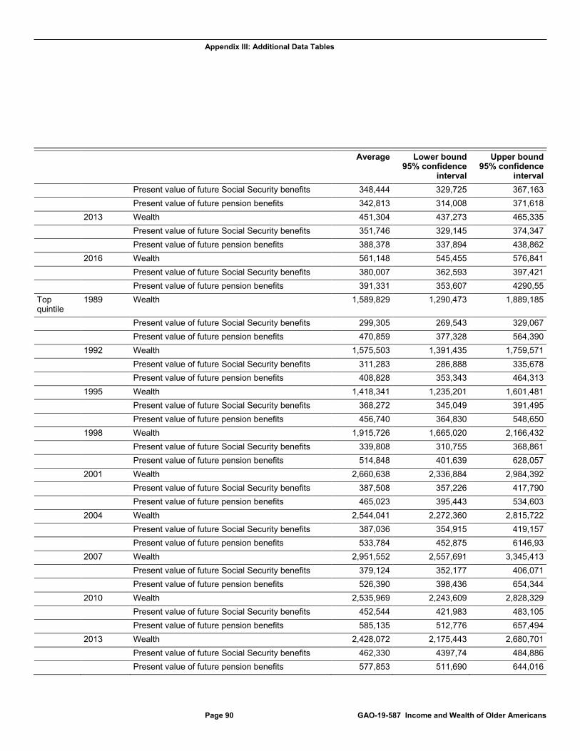
Appendix III: Additional Data Tables
Page 90 GAO-19-587 Income and Wealth of Older Americans
Average Lower bound 95% confidence
interval
Upper bound 95% confidence
interval Present value of future Social Security benefits 348,444 329,725 367,163 Present value of future pension benefits 342,813 314,008 371,618 2013 Wealth 451,304 437,273 465,335 Present value of future Social Security benefits 351,746 329,145 374,347 Present value of future pension benefits 388,378 337,894 438,862 2016 Wealth 561,148 545,455 576,841 Present value of future Social Security benefits 380,007 362,593 397,421 Present value of future pension benefits 391,331 353,607 4290,55 Top quintile
1989 Wealth 1,589,829 1,290,473 1,889,185
Present value of future Social Security benefits 299,305 269,543 329,067 Present value of future pension benefits 470,859 377,328 564,390 1992 Wealth 1,575,503 1,391,435 1,759,571 Present value of future Social Security benefits 311,283 286,888 335,678 Present value of future pension benefits 408,828 353,343 464,313 1995 Wealth 1,418,341 1,235,201 1,601,481 Present value of future Social Security benefits 368,272 345,049 391,495 Present value of future pension benefits 456,740 364,830 548,650 1998 Wealth 1,915,726 1,665,020 2,166,432 Present value of future Social Security benefits 339,808 310,755 368,861 Present value of future pension benefits 514,848 401,639 628,057 2001 Wealth 2,660,638 2,336,884 2,984,392 Present value of future Social Security benefits 387,508 357,226 417,790 Present value of future pension benefits 465,023 395,443 534,603 2004 Wealth 2,544,041 2,272,360 2,815,722 Present value of future Social Security benefits 387,036 354,915 419,157 Present value of future pension benefits 533,784 452,875 6146,93 2007 Wealth 2,951,552 2,557,691 3,345,413 Present value of future Social Security benefits 379,124 352,177 406,071 Present value of future pension benefits 526,390 398,436 654,344 2010 Wealth 2,535,969 2,243,609 2,828,329 Present value of future Social Security benefits 452,544 421,983 483,105 Present value of future pension benefits 585,135 512,776 657,494 2013 Wealth 2,428,072 2,175,443 2,680,701 Present value of future Social Security benefits 462,330 4397,74 484,886 Present value of future pension benefits 577,853 511,690 644,016
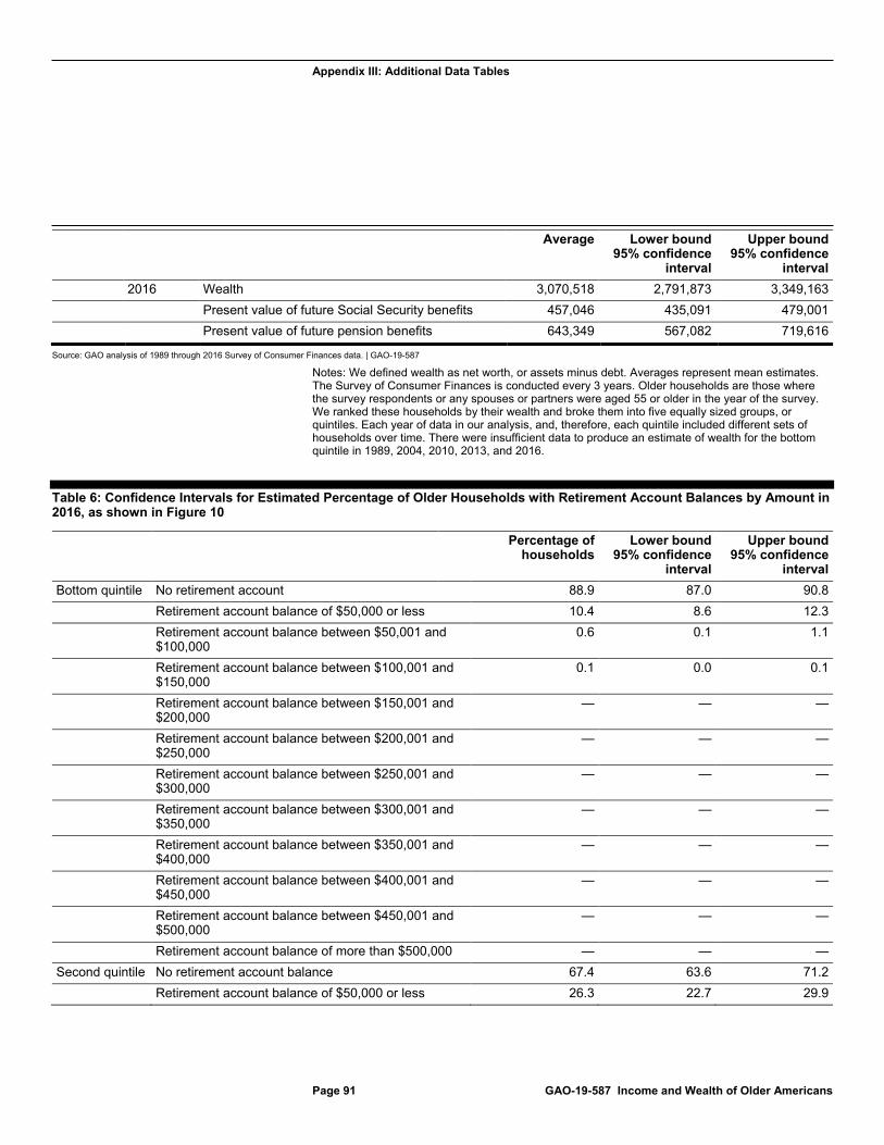
Appendix III: Additional Data Tables
Page 91 GAO-19-587 Income and Wealth of Older Americans
Average Lower bound 95% confidence
interval
Upper bound 95% confidence
interval 2016 Wealth 3,070,518 2,791,873 3,349,163 Present value of future Social Security benefits 457,046 435,091 479,001 Present value of future pension benefits 643,349 567,082 719,616
Source: GAO analysis of 1989 through 2016 Survey of Consumer Finances data. | GAO-19-587
Notes: We defined wealth as net worth, or assets minus debt. Averages represent mean estimates. The Survey of Consumer Finances is conducted every 3 years. Older households are those where the survey respondents or any spouses or partners were aged 55 or older in the year of the survey. We ranked these households by their wealth and broke them into five equally sized groups, or quintiles. Each year of data in our analysis, and, therefore, each quintile included different sets of households over time. There were insufficient data to produce an estimate of wealth for the bottom quintile in 1989, 2004, 2010, 2013, and 2016.
Table 6: Confidence Intervals for Estimated Percentage of Older Households with Retirement Account Balances by Amount in 2016, as shown in Figure 10
Percentage of households
Lower bound 95% confidence
interval
Upper bound 95% confidence
interval Bottom quintile No retirement account 88.9 87.0 90.8 Retirement account balance of $50,000 or less 10.4 8.6 12.3 Retirement account balance between $50,001 and
$100,000 0.6 0.1 1.1
Retirement account balance between $100,001 and $150,000
0.1 0.0 0.1
Retirement account balance between $150,001 and $200,000
— — —
Retirement account balance between $200,001 and $250,000
— — —
Retirement account balance between $250,001 and $300,000
— — —
Retirement account balance between $300,001 and $350,000
— — —
Retirement account balance between $350,001 and $400,000
— — —
Retirement account balance between $400,001 and $450,000
— — —
Retirement account balance between $450,001 and $500,000
— — —
Retirement account balance of more than $500,000 — — — Second quintile No retirement account balance 67.4 63.6 71.2 Retirement account balance of $50,000 or less 26.3 22.7 29.9
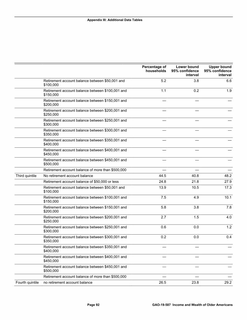
Appendix III: Additional Data Tables
Page 92 GAO-19-587 Income and Wealth of Older Americans
Percentage of households
Lower bound 95% confidence
interval
Upper bound 95% confidence
interval Retirement account balance between $50,001 and
$100,000 5.2 3.8 6.6
Retirement account balance between $100,001 and $150,000
1.1 0.2 1.9
Retirement account balance between $150,001 and $200,000
— — —
Retirement account balance between $200,001 and $250,000
— — —
Retirement account balance between $250,001 and $300,000
— — —
Retirement account balance between $300,001 and $350,000
— — —
Retirement account balance between $350,001 and $400,000
— — —
Retirement account balance between $400,001 and $450,000
— — —
Retirement account balance between $450,001 and $500,000
— — —
Retirement account balance of more than $500,000 — — — Third quintile No retirement account balance 44.5 40.8 48.2 Retirement account balance of $50,000 or less 24.8 21.8 27.9 Retirement account balance between $50,001 and
$100,000 13.9 10.5 17.3
Retirement account balance between $100,001 and $150,000
7.5 4.9 10.1
Retirement account balance between $150,001 and $200,000
5.8 3.8 7.8
Retirement account balance between $200,001 and $250,000
2.7 1.5 4.0
Retirement account balance between $250,001 and $300,000
0.6 0.0 1.2
Retirement account balance between $300,001 and $350,000
0.2 0.0 0.4
Retirement account balance between $350,001 and $400,000
— — —
Retirement account balance between $400,001 and $450,000
— — —
Retirement account balance between $450,001 and $500,000
— — —
Retirement account balance of more than $500,000 — — — Fourth quintile no retirement account balance 26.5 23.8 29.2
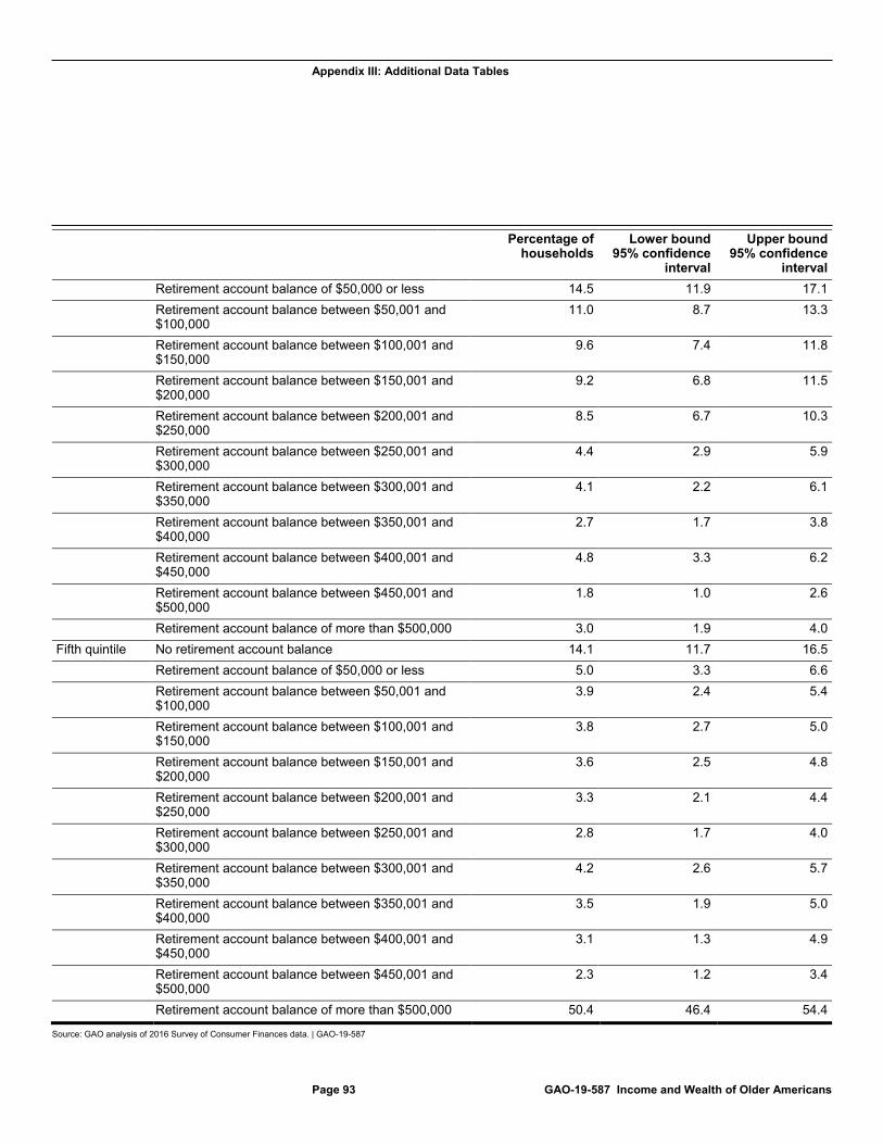
Appendix III: Additional Data Tables
Page 93 GAO-19-587 Income and Wealth of Older Americans
Percentage of households
Lower bound 95% confidence
interval
Upper bound 95% confidence
interval Retirement account balance of $50,000 or less 14.5 11.9 17.1 Retirement account balance between $50,001 and
$100,000 11.0 8.7 13.3
Retirement account balance between $100,001 and $150,000
9.6 7.4 11.8
Retirement account balance between $150,001 and $200,000
9.2 6.8 11.5
Retirement account balance between $200,001 and $250,000
8.5 6.7 10.3
Retirement account balance between $250,001 and $300,000
4.4 2.9 5.9
Retirement account balance between $300,001 and $350,000
4.1 2.2 6.1
Retirement account balance between $350,001 and $400,000
2.7 1.7 3.8
Retirement account balance between $400,001 and $450,000
4.8 3.3 6.2
Retirement account balance between $450,001 and $500,000
1.8 1.0 2.6
Retirement account balance of more than $500,000 3.0 1.9 4.0 Fifth quintile No retirement account balance 14.1 11.7 16.5 Retirement account balance of $50,000 or less 5.0 3.3 6.6 Retirement account balance between $50,001 and
$100,000 3.9 2.4 5.4
Retirement account balance between $100,001 and $150,000
3.8 2.7 5.0
Retirement account balance between $150,001 and $200,000
3.6 2.5 4.8
Retirement account balance between $200,001 and $250,000
3.3 2.1 4.4
Retirement account balance between $250,001 and $300,000
2.8 1.7 4.0
Retirement account balance between $300,001 and $350,000
4.2 2.6 5.7
Retirement account balance between $350,001 and $400,000
3.5 1.9 5.0
Retirement account balance between $400,001 and $450,000
3.1 1.3 4.9
Retirement account balance between $450,001 and $500,000
2.3 1.2 3.4
Retirement account balance of more than $500,000 50.4 46.4 54.4
Source: GAO analysis of 2016 Survey of Consumer Finances data. | GAO-19-587
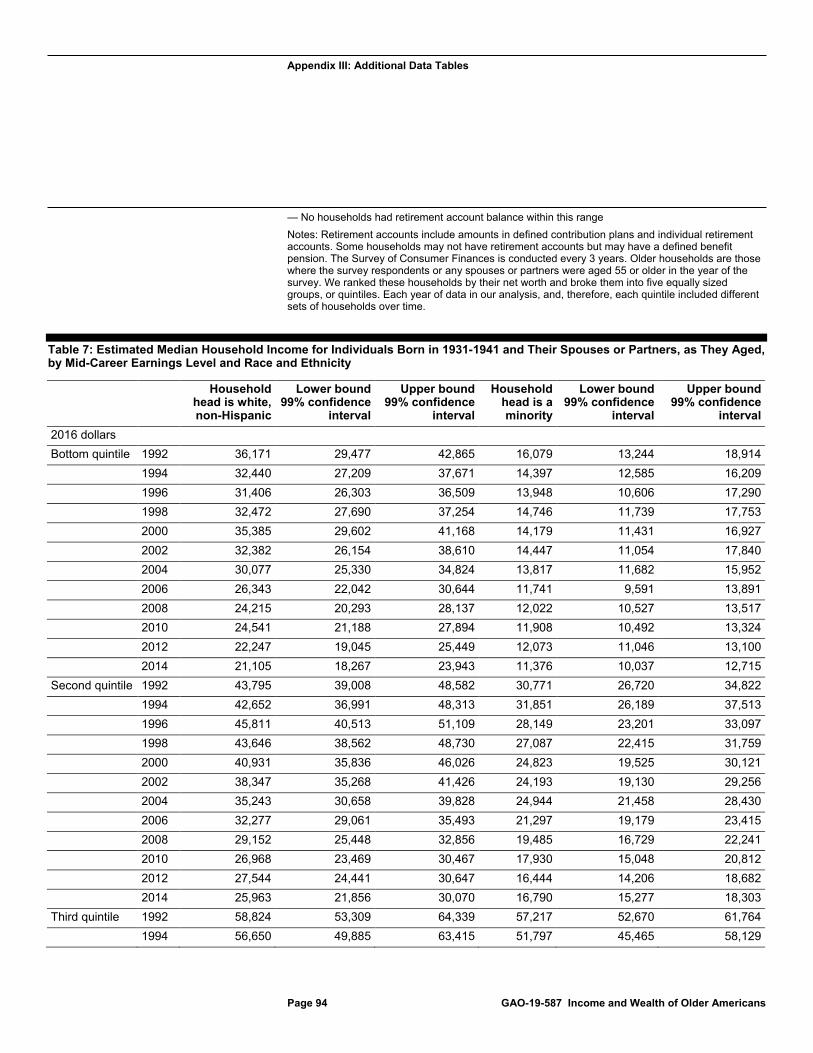
Appendix III: Additional Data Tables
Page 94 GAO-19-587 Income and Wealth of Older Americans
— No households had retirement account balance within this range Notes: Retirement accounts include amounts in defined contribution plans and individual retirement accounts. Some households may not have retirement accounts but may have a defined benefit pension. The Survey of Consumer Finances is conducted every 3 years. Older households are those where the survey respondents or any spouses or partners were aged 55 or older in the year of the survey. We ranked these households by their net worth and broke them into five equally sized groups, or quintiles. Each year of data in our analysis, and, therefore, each quintile included different sets of households over time.
Table 7: Estimated Median Household Income for Individuals Born in 1931-1941 and Their Spouses or Partners, as They Aged, by Mid-Career Earnings Level and Race and Ethnicity
Household head is white, non-Hispanic
Lower bound 99% confidence
interval
Upper bound 99% confidence
interval
Household head is a minority
Lower bound 99% confidence
interval
Upper bound 99% confidence
interval 2016 dollars Bottom quintile 1992 36,171 29,477 42,865 16,079 13,244 18,914 1994 32,440 27,209 37,671 14,397 12,585 16,209 1996 31,406 26,303 36,509 13,948 10,606 17,290 1998 32,472 27,690 37,254 14,746 11,739 17,753 2000 35,385 29,602 41,168 14,179 11,431 16,927 2002 32,382 26,154 38,610 14,447 11,054 17,840 2004 30,077 25,330 34,824 13,817 11,682 15,952 2006 26,343 22,042 30,644 11,741 9,591 13,891 2008 24,215 20,293 28,137 12,022 10,527 13,517 2010 24,541 21,188 27,894 11,908 10,492 13,324 2012 22,247 19,045 25,449 12,073 11,046 13,100 2014 21,105 18,267 23,943 11,376 10,037 12,715 Second quintile 1992 43,795 39,008 48,582 30,771 26,720 34,822 1994 42,652 36,991 48,313 31,851 26,189 37,513 1996 45,811 40,513 51,109 28,149 23,201 33,097 1998 43,646 38,562 48,730 27,087 22,415 31,759 2000 40,931 35,836 46,026 24,823 19,525 30,121 2002 38,347 35,268 41,426 24,193 19,130 29,256 2004 35,243 30,658 39,828 24,944 21,458 28,430 2006 32,277 29,061 35,493 21,297 19,179 23,415 2008 29,152 25,448 32,856 19,485 16,729 22,241 2010 26,968 23,469 30,467 17,930 15,048 20,812 2012 27,544 24,441 30,647 16,444 14,206 18,682 2014 25,963 21,856 30,070 16,790 15,277 18,303 Third quintile 1992 58,824 53,309 64,339 57,217 52,670 61,764 1994 56,650 49,885 63,415 51,797 45,465 58,129
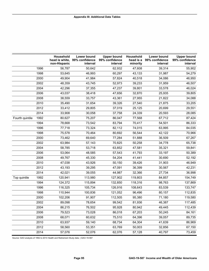
Appendix III: Additional Data Tables
Page 95 GAO-19-587 Income and Wealth of Older Americans
Household head is white, non-Hispanic
Lower bound 99% confidence
interval
Upper bound 99% confidence
interval
Household head is a minority
Lower bound 99% confidence
interval
Upper bound 99% confidence
interval 1996 56,787 50,642 62,932 47,608 39,314 55,902 1998 53,645 46,993 60,297 43,133 31,987 54,279 2000 49,904 41,984 57,824 40,518 34,086 46,950 2002 48,359 43,745 52,973 39,233 31,959 46,507 2004 42,296 37,355 47,237 39,801 33,578 46,024 2006 43,037 38,418 47,656 32,870 25,935 39,805 2008 38,559 33,757 43,361 27,955 21,822 34,088 2010 35,490 31,654 39,326 27,540 21,875 33,205 2012 33,412 29,805 37,019 25,125 20,699 29,551 2014 33,908 30,058 37,758 24,339 20,593 28,085 Fourth quintile 1992 80,627 75,207 86,047 77,568 67,712 87,424 1994 78,668 73,542 83,794 70,417 54,501 86,333 1996 77,718 73,324 82,112 74,015 63,995 84,035 1998 75,578 70,464 80,692 56,544 42,122 70,966 2000 73,462 69,640 77,284 51,888 36,509 67,267 2002 63,984 57,143 70,825 50,258 34,778 65,738 2004 58,785 53,718 63,852 47,581 35,321 59,841 2006 53,064 48,585 57,543 41,793 33,197 50,389 2008 49,767 45,330 54,204 41,441 30,690 52,192 2010 47,038 43,926 50,150 39,426 31,903 46,949 2012 43,193 39,295 47,091 36,399 30,567 42,231 2014 42,021 39,055 44,987 32,366 27,734 36,998 Top quintile 1992 120,941 113,980 127,902 119,803 84,857 154,749 1994 124,372 115,894 132,850 118,316 98,763 137,869 1996 116,325 105,734 126,916 108,643 83,539 133,747 1998 110,944 100,836 121,052 96,496 80,157 112,835 2000 102,206 91,907 112,505 95,380 71,180 119,580 2002 89,098 78,654 99,542 81,936 46,387 117,485 2004 86,215 76,502 95,928 80,942 49,445 112,439 2006 79,523 73,028 86,018 67,203 50,245 84,161 2008 68,071 60,632 75,510 64,396 39,057 89,735 2010 63,937 59,140 68,734 64,304 41,639 86,969 2012 58,560 53,351 63,769 50,003 32,856 67,150 2014 57,076 52,076 62,076 57,128 40,797 73,459
Source: GAO analysis of 1992 to 2014 Health and Retirement Study data. | GAO-19-587
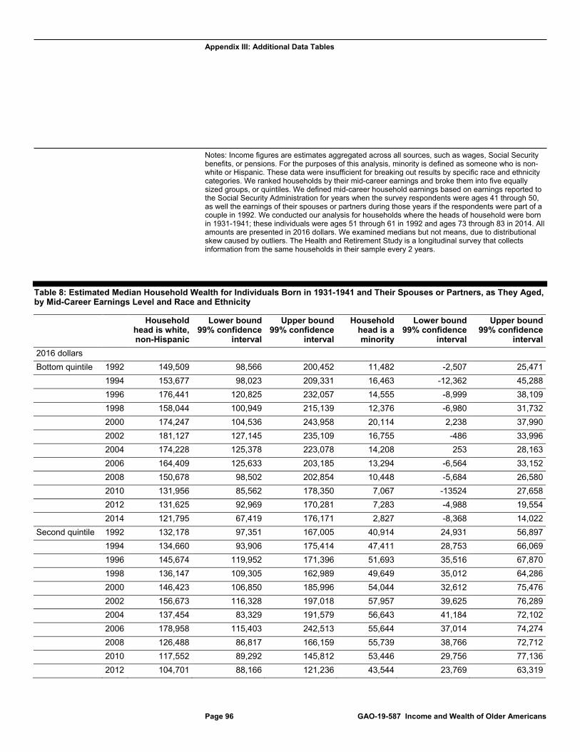
Appendix III: Additional Data Tables
Page 96 GAO-19-587 Income and Wealth of Older Americans
Notes: Income figures are estimates aggregated across all sources, such as wages, Social Security benefits, or pensions. For the purposes of this analysis, minority is defined as someone who is non-white or Hispanic. These data were insufficient for breaking out results by specific race and ethnicity categories. We ranked households by their mid-career earnings and broke them into five equally sized groups, or quintiles. We defined mid-career household earnings based on earnings reported to the Social Security Administration for years when the survey respondents were ages 41 through 50, as well the earnings of their spouses or partners during those years if the respondents were part of a couple in 1992. We conducted our analysis for households where the heads of household were born in 1931-1941; these individuals were ages 51 through 61 in 1992 and ages 73 through 83 in 2014. All amounts are presented in 2016 dollars. We examined medians but not means, due to distributional skew caused by outliers. The Health and Retirement Study is a longitudinal survey that collects information from the same households in their sample every 2 years.
Table 8: Estimated Median Household Wealth for Individuals Born in 1931-1941 and Their Spouses or Partners, as They Aged, by Mid-Career Earnings Level and Race and Ethnicity
Household head is white, non-Hispanic
Lower bound 99% confidence
interval
Upper bound 99% confidence
interval
Household head is a minority
Lower bound 99% confidence
interval
Upper bound 99% confidence
interval 2016 dollars Bottom quintile 1992 149,509 98,566 200,452 11,482 -2,507 25,471 1994 153,677 98,023 209,331 16,463 -12,362 45,288 1996 176,441 120,825 232,057 14,555 -8,999 38,109 1998 158,044 100,949 215,139 12,376 -6,980 31,732 2000 174,247 104,536 243,958 20,114 2,238 37,990 2002 181,127 127,145 235,109 16,755 -486 33,996 2004 174,228 125,378 223,078 14,208 253 28,163 2006 164,409 125,633 203,185 13,294 -6,564 33,152 2008 150,678 98,502 202,854 10,448 -5,684 26,580 2010 131,956 85,562 178,350 7,067 -13524 27,658 2012 131,625 92,969 170,281 7,283 -4,988 19,554 2014 121,795 67,419 176,171 2,827 -8,368 14,022 Second quintile 1992 132,178 97,351 167,005 40,914 24,931 56,897 1994 134,660 93,906 175,414 47,411 28,753 66,069 1996 145,674 119,952 171,396 51,693 35,516 67,870 1998 136,147 109,305 162,989 49,649 35,012 64,286 2000 146,423 106,850 185,996 54,044 32,612 75,476 2002 156,673 116,328 197,018 57,957 39,625 76,289 2004 137,454 83,329 191,579 56,643 41,184 72,102 2006 178,958 115,403 242,513 55,644 37,014 74,274 2008 126,488 86,817 166,159 55,739 38,766 72,712 2010 117,552 89,292 145,812 53,446 29,756 77,136 2012 104,701 88,166 121,236 43,544 23,769 63,319
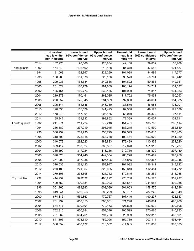
Appendix III: Additional Data Tables
Page 97 GAO-19-587 Income and Wealth of Older Americans
Household head is white, non-Hispanic
Lower bound 99% confidence
interval
Upper bound 99% confidence
interval
Household head is a minority
Lower bound 99% confidence
interval
Upper bound 99% confidence
interval 2014 107,975 90,066 125,884 42,160 29,052 55,268 Third quintile 1992 174,340 136,492 212,188 84,370 47,553 121,187 1994 191,068 152,867 229,269 101,038 84,699 117,377 1996 188,906 151,676 226,136 98,573 50,704 146,442 1998 209,035 168,534 249,536 104,602 59,853 149,351 2000 231,324 180,779 281,869 103,174 74,711 131,637 2002 195,454 160,773 230,135 101,900 71,817 131,983 2004 219,273 170,461 268,085 117,752 75,451 160,053 2006 230,352 175,845 284,859 97,838 40,691 154,985 2008 205,144 161,538 248,750 87,576 46,951 128.201 2010 198,536 155,579 241,493 89,358 49,177 129.539 2012 178,043 147,901 208,185 68,070 38,329 97.811 2014 165,342 131,832 198,852 72,359 43,007 101.711 Fourth quintile 1992 241.971 211,724 272,218 154,451 103,788 205,114 1994 266.582 237,219 295,945 183,215 113,590 252,840 1996 306.232 261,735 350,729 199,549 130,615 268,483 1998 318.693 273,618 363,768 199,451 153,922 244,980 2000 340.673 292,523 388,823 172,439 110,358 234,520 2002 339.417 293,027 385,807 212,078 151,919 272,237 2004 365.590 317,924 413,256 212,750 128,370 297,130 2006 378.525 314,746 442,304 266,220 138,482 393,958 2008 371.292 317,088 425,496 244,855 129,365 360,345 2010 310.035 261,123 358,947 191,032 136,342 245,722 2012 273.186 221,367 325,005 153,613 112,454 194,772 2014 279.105 233,898 324,312 170,645 126,252 215,038 Top quintile 1992 444,257 3922,22 496,292 273,760 194,523 352,997 1994 499,552 429,181 569,923 366,547 241,056 492,038 1996 551,466 493,843 609,089 301,603 158,570 444,636 1998 619,941 559,653 680,229 353,797 287,245 420,349 2000 674,815 569,863 779,767 307,440 190,237 424,643 2002 701,992 618,353 785,631 371,296 246,604 495,988 2004 684,677 599,191 770,163 321,820 153,032 490,608 2006 752,315 650,284 854,346 405,599 270,465 540,733 2008 701,262 604,761 797,763 323,909 182,317 465,501 2010 641,303 523,510 759,096 352,789 207,114 498,464 2012 586,852 460,172 713,532 214,865 121,857 307,873
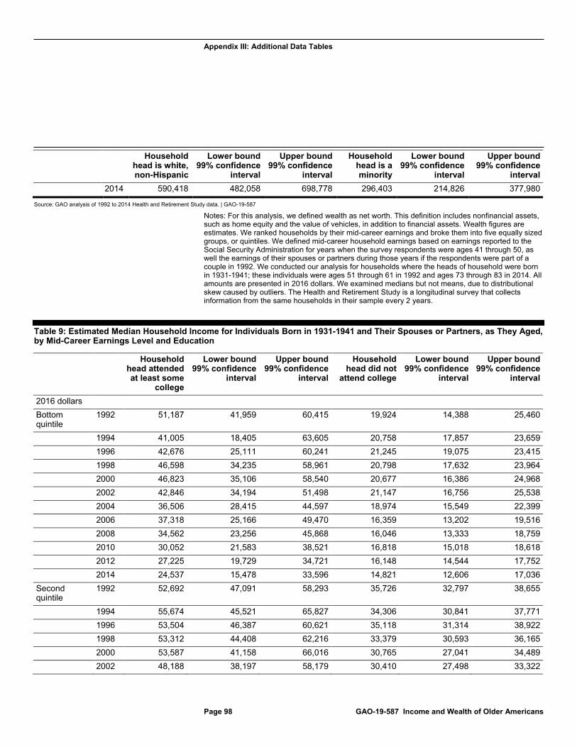
Appendix III: Additional Data Tables
Page 98 GAO-19-587 Income and Wealth of Older Americans
Household head is white, non-Hispanic
Lower bound 99% confidence
interval
Upper bound 99% confidence
interval
Household head is a minority
Lower bound 99% confidence
interval
Upper bound 99% confidence
interval 2014 590,418 482,058 698,778 296,403 214,826 377,980
Source: GAO analysis of 1992 to 2014 Health and Retirement Study data. | GAO-19-587
Notes: For this analysis, we defined wealth as net worth. This definition includes nonfinancial assets, such as home equity and the value of vehicles, in addition to financial assets. Wealth figures are estimates. We ranked households by their mid-career earnings and broke them into five equally sized groups, or quintiles. We defined mid-career household earnings based on earnings reported to the Social Security Administration for years when the survey respondents were ages 41 through 50, as well the earnings of their spouses or partners during those years if the respondents were part of a couple in 1992. We conducted our analysis for households where the heads of household were born in 1931-1941; these individuals were ages 51 through 61 in 1992 and ages 73 through 83 in 2014. All amounts are presented in 2016 dollars. We examined medians but not means, due to distributional skew caused by outliers. The Health and Retirement Study is a longitudinal survey that collects information from the same households in their sample every 2 years.
Table 9: Estimated Median Household Income for Individuals Born in 1931-1941 and Their Spouses or Partners, as They Aged, by Mid-Career Earnings Level and Education
Household head attended at least some
college
Lower bound 99% confidence
interval
Upper bound 99% confidence
interval
Household head did not
attend college
Lower bound 99% confidence
interval
Upper bound 99% confidence
interval
2016 dollars Bottom quintile
1992 51,187 41,959 60,415 19,924 14,388 25,460
1994 41,005 18,405 63,605 20,758 17,857 23,659 1996 42,676 25,111 60,241 21,245 19,075 23,415 1998 46,598 34,235 58,961 20,798 17,632 23,964 2000 46,823 35,106 58,540 20,677 16,386 24,968 2002 42,846 34,194 51,498 21,147 16,756 25,538 2004 36,506 28,415 44,597 18,974 15,549 22,399 2006 37,318 25,166 49,470 16,359 13,202 19,516 2008 34,562 23,256 45,868 16,046 13,333 18,759 2010 30,052 21,583 38,521 16,818 15,018 18,618 2012 27,225 19,729 34,721 16,148 14,544 17,752 2014 24,537 15,478 33,596 14,821 12,606 17,036 Second quintile
1992 52,692 47,091 58,293 35,726 32,797 38,655
1994 55,674 45,521 65,827 34,306 30,841 37,771 1996 53,504 46,387 60,621 35,118 31,314 38,922 1998 53,312 44,408 62,216 33,379 30,593 36,165 2000 53,587 41,158 66,016 30,765 27,041 34,489 2002 48,188 38,197 58,179 30,410 27,498 33,322
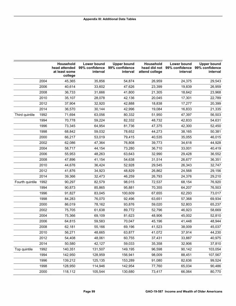
Appendix III: Additional Data Tables
Page 99 GAO-19-587 Income and Wealth of Older Americans
Household head attended at least some
college
Lower bound 99% confidence
interval
Upper bound 99% confidence
interval
Household head did not
attend college
Lower bound 99% confidence
interval
Upper bound 99% confidence
interval
2004 45,365 35,856 54,874 26,959 24,375 29,543 2006 40,614 33,602 47,626 23,399 19,839 26,959 2008 36,733 31,666 41,800 21,305 18,642 23,968 2010 35,107 28,078 42,136 20,045 17,301 22,789 2012 37,904 32,920 42,888 18,838 17,277 20,399 2014 36,570 30,144 42,996 19,084 16,833 21,335 Third quintile 1992 71,694 63,056 80,332 51,950 47,397 56,503 1994 70,778 59,224 82,332 48,732 42,833 54,631 1996 73,345 64,954 81,736 47,375 42,300 52,450 1998 68,842 59,032 78,652 44,273 38,165 50,381 2000 66,217 53,019 79,415 40,535 35,055 46,015 2002 62,086 47,364 76,808 39,773 34,618 44,928 2004 58,717 44,154 73,280 36,710 33,001 40,419 2006 55,953 48,263 63,643 32,990 29,428 36,552 2008 47,896 41,154 54,638 31,514 26,677 36,351 2010 44,676 36,424 52,928 29,545 26,343 32,747 2012 41,876 34,923 48,829 26,862 24,568 29,156 2014 39,366 32,473 46,259 26,793 24,376 29,210 Fourth quintile 1992 90,297 82,579 98,015 72,537 68,154 76,920 1994 90,873 85,865 95,881 70,355 64,207 76,503 1996 91,827 83,045 100,609 67,655 62,293 73,017 1998 84,283 76,070 92,496 63,651 57,368 69,934 2000 86,019 78,162 93,876 59,020 52,803 65,237 2002 75,705 61,638 89,772 52,796 46,923 58,669 2004 75,366 69,109 81,623 48,906 45,002 52,810 2006 64,815 59,583 70,047 45,196 41,448 48,944 2008 62,181 55,166 69,196 41,523 38,009 45,037 2010 56,271 48,665 63,877 41,072 37,914 44,230 2012 54,408 48,061 60,755 37,431 33,887 40,975 2014 50,580 42,127 59,033 35,358 32,906 37,810 Top quintile 1992 140,351 131,507 149,195 96,598 90,142 103,054 1994 142,950 128,959 156,941 98,009 88,451 107,567 1996 139,212 125,135 153,289 91,080 82,636 99,524 1998 128,950 114,946 142,954 77,760 65,034 90,486 2000 118,112 105,544 130,680 73,417 66,064 80,770
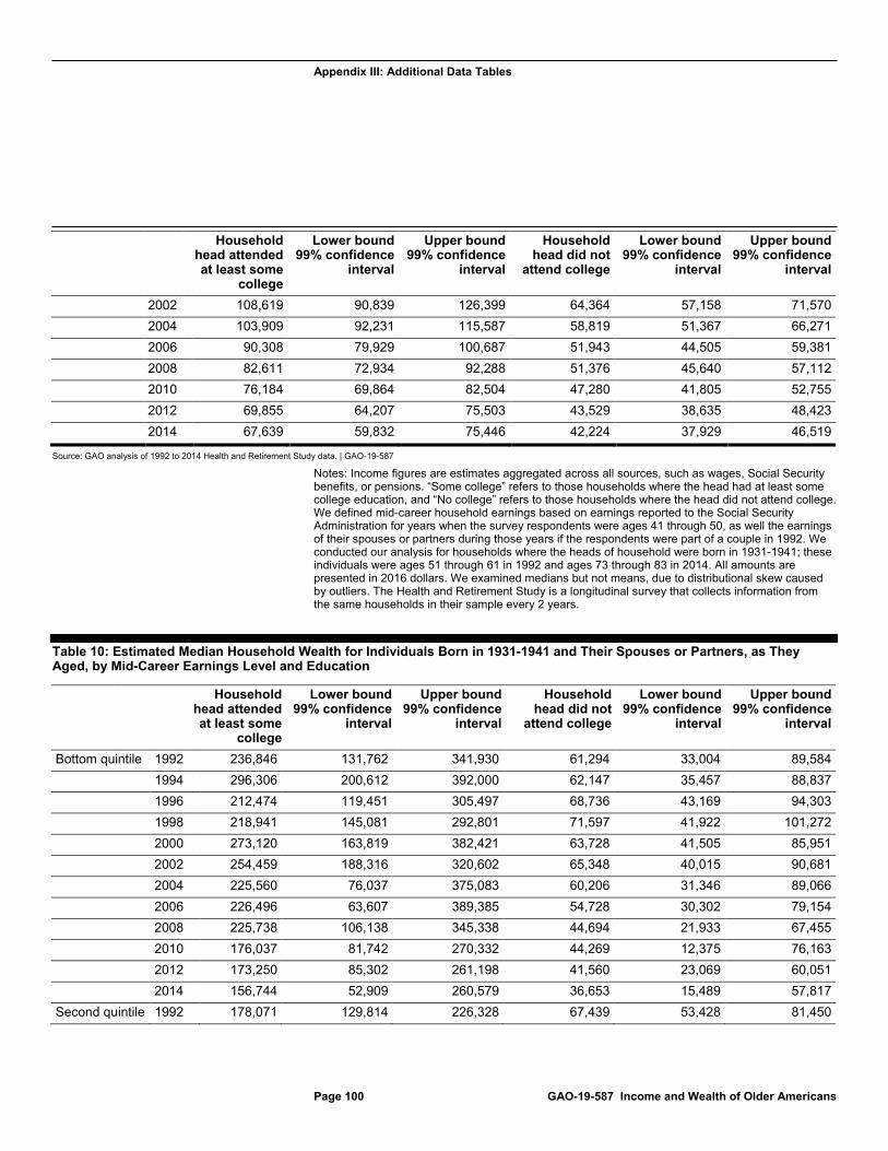
Appendix III: Additional Data Tables
Page 100 GAO-19-587 Income and Wealth of Older Americans
Household head attended at least some
college
Lower bound 99% confidence
interval
Upper bound 99% confidence
interval
Household head did not
attend college
Lower bound 99% confidence
interval
Upper bound 99% confidence
interval
2002 108,619 90,839 126,399 64,364 57,158 71,570 2004 103,909 92,231 115,587 58,819 51,367 66,271 2006 90,308 79,929 100,687 51,943 44,505 59,381 2008 82,611 72,934 92,288 51,376 45,640 57,112 2010 76,184 69,864 82,504 47,280 41,805 52,755 2012 69,855 64,207 75,503 43,529 38,635 48,423 2014 67,639 59,832 75,446 42,224 37,929 46,519
Source: GAO analysis of 1992 to 2014 Health and Retirement Study data. | GAO-19-587
Notes: Income figures are estimates aggregated across all sources, such as wages, Social Security benefits, or pensions. “Some college” refers to those households where the head had at least some college education, and “No college” refers to those households where the head did not attend college. We defined mid-career household earnings based on earnings reported to the Social Security Administration for years when the survey respondents were ages 41 through 50, as well the earnings of their spouses or partners during those years if the respondents were part of a couple in 1992. We conducted our analysis for households where the heads of household were born in 1931-1941; these individuals were ages 51 through 61 in 1992 and ages 73 through 83 in 2014. All amounts are presented in 2016 dollars. We examined medians but not means, due to distributional skew caused by outliers. The Health and Retirement Study is a longitudinal survey that collects information from the same households in their sample every 2 years.
Table 10: Estimated Median Household Wealth for Individuals Born in 1931-1941 and Their Spouses or Partners, as They Aged, by Mid-Career Earnings Level and Education
Household head attended at least some
college
Lower bound 99% confidence
interval
Upper bound 99% confidence
interval
Household head did not
attend college
Lower bound 99% confidence
interval
Upper bound 99% confidence
interval
Bottom quintile 1992 236,846 131,762 341,930 61,294 33,004 89,584 1994 296,306 200,612 392,000 62,147 35,457 88,837 1996 212,474 119,451 305,497 68,736 43,169 94,303 1998 218,941 145,081 292,801 71,597 41,922 101,272 2000 273,120 163,819 382,421 63,728 41,505 85,951 2002 254,459 188,316 320,602 65,348 40,015 90,681 2004 225,560 76,037 375,083 60,206 31,346 89,066 2006 226,496 63,607 389,385 54,728 30,302 79,154 2008 225,738 106,138 345,338 44,694 21,933 67,455 2010 176,037 81,742 270,332 44,269 12,375 76,163 2012 173,250 85,302 261,198 41,560 23,069 60,051 2014 156,744 52,909 260,579 36,653 15,489 57,817 Second quintile 1992 178,071 129,814 226,328 67,439 53,428 81,450
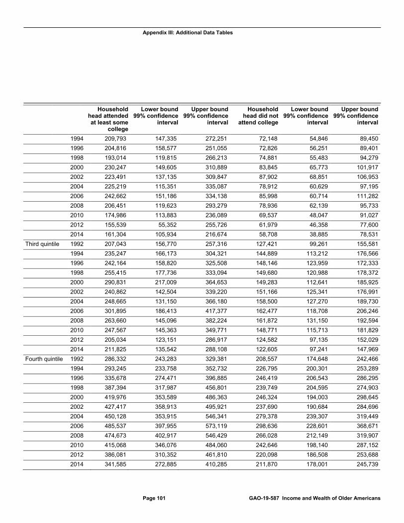
Appendix III: Additional Data Tables
Page 101 GAO-19-587 Income and Wealth of Older Americans
Household head attended at least some
college
Lower bound 99% confidence
interval
Upper bound 99% confidence
interval
Household head did not
attend college
Lower bound 99% confidence
interval
Upper bound 99% confidence
interval
1994 209,793 147,335 272,251 72,148 54,846 89,450 1996 204,816 158,577 251,055 72,826 56,251 89,401 1998 193,014 119,815 266,213 74,881 55,483 94,279 2000 230,247 149,605 310,889 83,845 65,773 101,917 2002 223,491 137,135 309,847 87,902 68,851 106,953 2004 225,219 115,351 335,087 78,912 60,629 97,195 2006 242,662 151,186 334,138 85,998 60,714 111,282 2008 206,451 119,623 293,279 78,936 62,139 95,733 2010 174,986 113,883 236,089 69,537 48,047 91,027 2012 155,539 55,352 255,726 61,979 46,358 77,600 2014 161,304 105,934 216,674 58,708 38,885 78,531 Third quintile 1992 207,043 156,770 257,316 127,421 99,261 155,581 1994 235,247 166,173 304,321 144,889 113,212 176,566 1996 242,164 158,820 325,508 148,146 123,959 172,333 1998 255,415 177,736 333,094 149,680 120,988 178,372 2000 290,831 217,009 364,653 149,283 112,641 185,925 2002 240,862 142,504 339,220 151,166 125,341 176,991 2004 248,665 131,150 366,180 158,500 127,270 189,730 2006 301,895 186,413 417,377 162,477 118,708 206,246 2008 263,660 145,096 382,224 161,872 131,150 192,594 2010 247,567 145,363 349,771 148,771 115,713 181,829 2012 205,034 123,151 286,917 124,582 97,135 152,029 2014 211,825 135,542 288,108 122,605 97,241 147,969 Fourth quintile 1992 286,332 243,283 329,381 208,557 174,648 242,466 1994 293,245 233,758 352,732 226,795 200,301 253,289 1996 335,678 274,471 396,885 246,419 206,543 286,295 1998 387,394 317,987 456,801 239,749 204,595 274,903 2000 419,976 353,589 486,363 246,324 194,003 298,645 2002 427,417 358,913 495,921 237,690 190,684 284,696 2004 450,128 353,915 546,341 279,378 239,307 319,449 2006 485,537 397,955 573,119 298,636 228,601 368,671 2008 474,673 402,917 546,429 266,028 212,149 319,907 2010 415,068 346,076 484,060 242,646 198,140 287,152 2012 386,081 310,352 461,810 220,098 186,508 253,688 2014 341,585 272,885 410,285 211,870 178,001 245,739
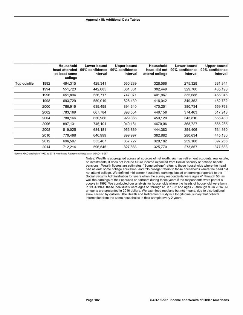
Appendix III: Additional Data Tables
Page 102 GAO-19-587 Income and Wealth of Older Americans
Household head attended at least some
college
Lower bound 99% confidence
interval
Upper bound 99% confidence
interval
Household head did not
attend college
Lower bound 99% confidence
interval
Upper bound 99% confidence
interval
Top quintile 1992 494,315 428,341 560,289 328,586 275,328 381,844 1994 551,723 442,085 661,361 382,449 329,700 435,198 1996 651,894 556,717 747,071 401,867 335,688 468,046 1998 693,729 559,019 828,439 416,042 349,352 482,732 2000 766,919 639,498 894,340 470,251 380,734 559,768 2002 783,169 667,784 898,554 446,158 374,403 517,913 2004 780,166 630,966 929,366 450,120 343,810 556,430 2006 897,131 745,101 1,049,161 4670,06 368,727 565,285 2008 819,025 684,181 953,869 444,383 354,406 534,360 2010 770,498 640,999 899,997 362,882 280,634 445,130 2012 696,597 555,467 837,727 328,182 259,108 397,256 2014 712,214 596,545 827,883 325,770 273,857 377,683
Source: GAO analysis of 1992 to 2014 Health and Retirement Study data. | GAO-19-587
Notes: Wealth is aggregated across all sources of net worth, such as retirement accounts, real estate, or investments. It does not include future income expected from Social Security or defined benefit pensions. Wealth figures are estimates. “Some college” refers to those households where the head had at least some college education, and “No college” refers to those households where the head did not attend college. We defined mid-career household earnings based on earnings reported to the Social Security Administration for years when the survey respondents were ages 41 through 50, as well the earnings of their spouses or partners during those years if the respondents were part of a couple in 1992. We conducted our analysis for households where the heads of household were born in 1931-1941; these individuals were ages 51 through 61 in 1992 and ages 73 through 83 in 2014. All amounts are presented in 2016 dollars. We examined medians but not means, due to distributional skew caused by outliers. The Health and Retirement Study is a longitudinal survey that collects information from the same households in their sample every 2 years.
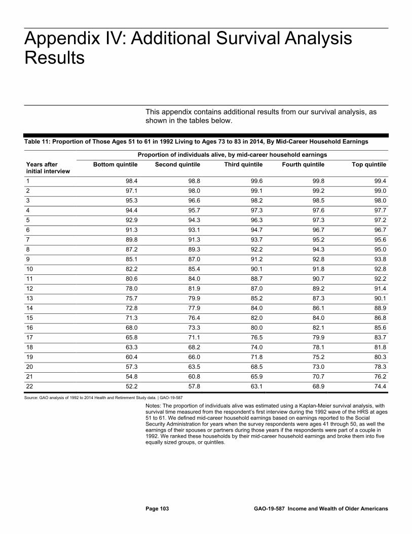
Appendix IV: Additional Survival Analysis Results
Page 103 GAO-19-587 Income and Wealth of Older Americans
This appendix contains additional results from our survival analysis, as shown in the tables below.
Table 11: Proportion of Those Ages 51 to 61 in 1992 Living to Ages 73 to 83 in 2014, By Mid-Career Household Earnings
Proportion of individuals alive, by mid-career household earnings Years after initial interview
Bottom quintile Second quintile Third quintile Fourth quintile Top quintile
1 98.4 98.8 99.6 99.8 99.4 2 97.1 98.0 99.1 99.2 99.0 3 95.3 96.6 98.2 98.5 98.0 4 94.4 95.7 97.3 97.6 97.7 5 92.9 94.3 96.3 97.3 97.2 6 91.3 93.1 94.7 96.7 96.7 7 89.8 91.3 93.7 95.2 95.6 8 87.2 89.3 92.2 94.3 95.0 9 85.1 87.0 91.2 92.8 93.8 10 82.2 85.4 90.1 91.8 92.8 11 80.6 84.0 88.7 90.7 92.2 12 78.0 81.9 87.0 89.2 91.4 13 75.7 79.9 85.2 87.3 90.1 14 72.8 77.9 84.0 86.1 88.9 15 71.3 76.4 82.0 84.0 86.8 16 68.0 73.3 80.0 82.1 85.6 17 65.8 71.1 76.5 79.9 83.7 18 63.3 68.2 74.0 78.1 81.8 19 60.4 66.0 71.8 75.2 80.3 20 57.3 63.5 68.5 73.0 78.3 21 54.8 60.8 65.9 70.7 76.2 22 52.2 57.8 63.1 68.9 74.4
Source: GAO analysis of 1992 to 2014 Health and Retirement Study data. | GAO-19-587
Notes: The proportion of individuals alive was estimated using a Kaplan-Meier survival analysis, with survival time measured from the respondent’s first interview during the 1992 wave of the HRS at ages 51 to 61. We defined mid-career household earnings based on earnings reported to the Social Security Administration for years when the survey respondents were ages 41 through 50, as well the earnings of their spouses or partners during those years if the respondents were part of a couple in 1992. We ranked these households by their mid-career household earnings and broke them into five equally sized groups, or quintiles.
Appendix IV: Additional Survival Analysis Results
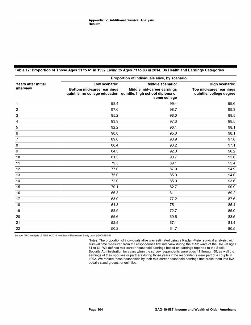
Appendix IV: Additional Survival Analysis Results
Page 104 GAO-19-587 Income and Wealth of Older Americans
Table 12: Proportion of Those Ages 51 to 61 in 1992 Living to Ages 73 to 83 in 2014, By Health and Earnings Categories
Proportion of individuals alive, by scenario Years after initial interview
Low scenario: Bottom mid-career earnings
quintile, no college education
Middle scenario: Middle mid-career earnings
quintile, high school diploma or some college
High scenario: Top mid-career earnings
quintile, college degree
1 98.4 99.4 99.6 2 97.0 98.7 99.3 3 95.2 98.0 98.5 4 93.9 97.3 98.5 5 92.2 96.1 98.1 6 90.8 95.0 98.1 7 89.0 93.9 97.8 8 86.4 93.2 97.1 9 84.3 92.0 96.2 10 81.3 90.7 95.6 11 79.3 89.1 95.4 12 77.0 87.9 94.9 13 75.0 85.9 94.0 14 72.0 85.0 93.6 15 70.1 82.7 90.9 16 66.3 81.1 89.2 17 63.9 77.2 87.6 18 61.8 75.1 85.4 19 58.9 72.7 85.0 20 55.6 69.6 83.5 21 52.5 67.1 81.4 22 50.2 64.7 80.5
Source: GAO analysis of 1992 to 2014 Health and Retirement Study data. | GAO-19-587
Notes: The proportion of individuals alive was estimated using a Kaplan-Meier survival analysis, with survival time measured from the respondent’s first interview during the 1992 wave of the HRS at ages 51 to 61. We defined mid-career household earnings based on earnings reported to the Social Security Administration for years when the survey respondents were ages 41 through 50, as well the earnings of their spouses or partners during those years if the respondents were part of a couple in 1992. We ranked these households by their mid-career household earnings and broke them into five equally sized groups, or quintiles.
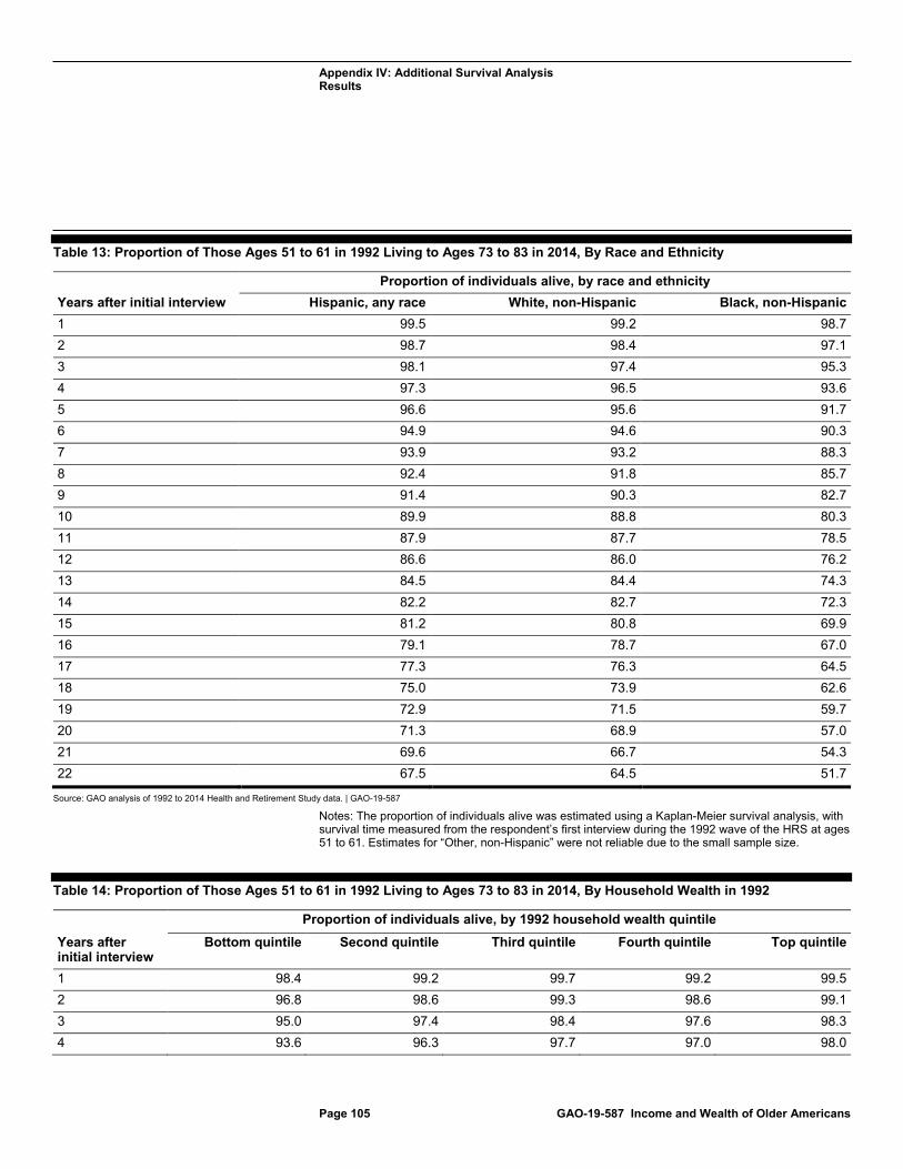
Appendix IV: Additional Survival Analysis Results
Page 105 GAO-19-587 Income and Wealth of Older Americans
Table 13: Proportion of Those Ages 51 to 61 in 1992 Living to Ages 73 to 83 in 2014, By Race and Ethnicity
Proportion of individuals alive, by race and ethnicity Years after initial interview Hispanic, any race White, non-Hispanic Black, non-Hispanic 1 99.5 99.2 98.7 2 98.7 98.4 97.1 3 98.1 97.4 95.3 4 97.3 96.5 93.6 5 96.6 95.6 91.7 6 94.9 94.6 90.3 7 93.9 93.2 88.3 8 92.4 91.8 85.7 9 91.4 90.3 82.7 10 89.9 88.8 80.3 11 87.9 87.7 78.5 12 86.6 86.0 76.2 13 84.5 84.4 74.3 14 82.2 82.7 72.3 15 81.2 80.8 69.9 16 79.1 78.7 67.0 17 77.3 76.3 64.5 18 75.0 73.9 62.6 19 72.9 71.5 59.7 20 71.3 68.9 57.0 21 69.6 66.7 54.3 22 67.5 64.5 51.7
Source: GAO analysis of 1992 to 2014 Health and Retirement Study data. | GAO-19-587
Notes: The proportion of individuals alive was estimated using a Kaplan-Meier survival analysis, with survival time measured from the respondent’s first interview during the 1992 wave of the HRS at ages 51 to 61. Estimates for “Other, non-Hispanic” were not reliable due to the small sample size.
Table 14: Proportion of Those Ages 51 to 61 in 1992 Living to Ages 73 to 83 in 2014, By Household Wealth in 1992
Proportion of individuals alive, by 1992 household wealth quintile Years after initial interview
Bottom quintile Second quintile Third quintile Fourth quintile Top quintile
1 98.4 99.2 99.7 99.2 99.5 2 96.8 98.6 99.3 98.6 99.1 3 95.0 97.4 98.4 97.6 98.3 4 93.6 96.3 97.7 97.0 98.0
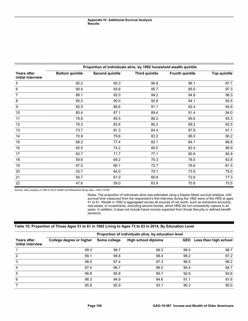
Appendix IV: Additional Survival Analysis Results
Page 106 GAO-19-587 Income and Wealth of Older Americans
Proportion of individuals alive, by 1992 household wealth quintile Years after initial interview
Bottom quintile Second quintile Third quintile Fourth quintile Top quintile
5 92.2 95.3 96.8 96.1 97.7 6 90.4 93.6 95.7 95.5 97.3 7 88.1 92.0 94.2 94.8 96.3 8 85.5 90.0 92.8 94.1 95.5 9 82.9 88.6 91.1 92.4 94.9 10 80.4 87.1 89.4 91.4 94.0 11 78.8 85.5 88.2 90.6 93.3 12 76.3 83.6 86.2 89.2 92.5 13 73.7 81.3 84.4 87.8 91.1 14 70.9 79.6 83.2 86.0 90.2 15 68.2 77.4 82.1 84.1 88.8 16 65.5 74.2 80.0 82.4 86.9 17 62.7 71.7 77.1 80.8 84.9 18 59.6 69.2 75.3 78.5 82.8 19 57.0 66.1 72.7 76.6 81.5 20 53.7 64.0 70.1 73.9 79.0 21 50.7 61.0 66.8 72.6 77.3 22 47.6 59.0 63.9 70.8 75.5
Source: GAO analysis of 1992 to 2014 Health and Retirement Study data. | GAO-19-587
Notes: The proportion of individuals alive was estimated using a Kaplan-Meier survival analysis, with survival time measured from the respondent’s first interview during the 1992 wave of the HRS at ages 51 to 61. Wealth in 1992 is aggregated across all sources of net worth, such as retirement accounts, real estate, or investments, excluding second homes, which HRS did not consistently capture in all years. In addition, it does not include future income expected from Social Security or defined benefit pensions.
Table 15: Proportion of Those Ages 51 to 61 in 1992 Living to Ages 73 to 83 in 2014, By Education Level
Proportion of individuals alive, by education level Years after initial interview
College degree or higher Some college High school diploma GED Less than high school
1 99.3 99.7 99.3 99.0 98.7 2 99.1 98.8 98.4 98.2 97.2 3 98.0 97.4 97.3 96.5 96.2 4 97.4 96.7 96.5 95.4 94.7 5 96.8 95.8 95.7 92.6 93.6 6 96.3 94.9 94.6 91.1 91.6 7 95.8 92.9 93.1 90.3 90.0
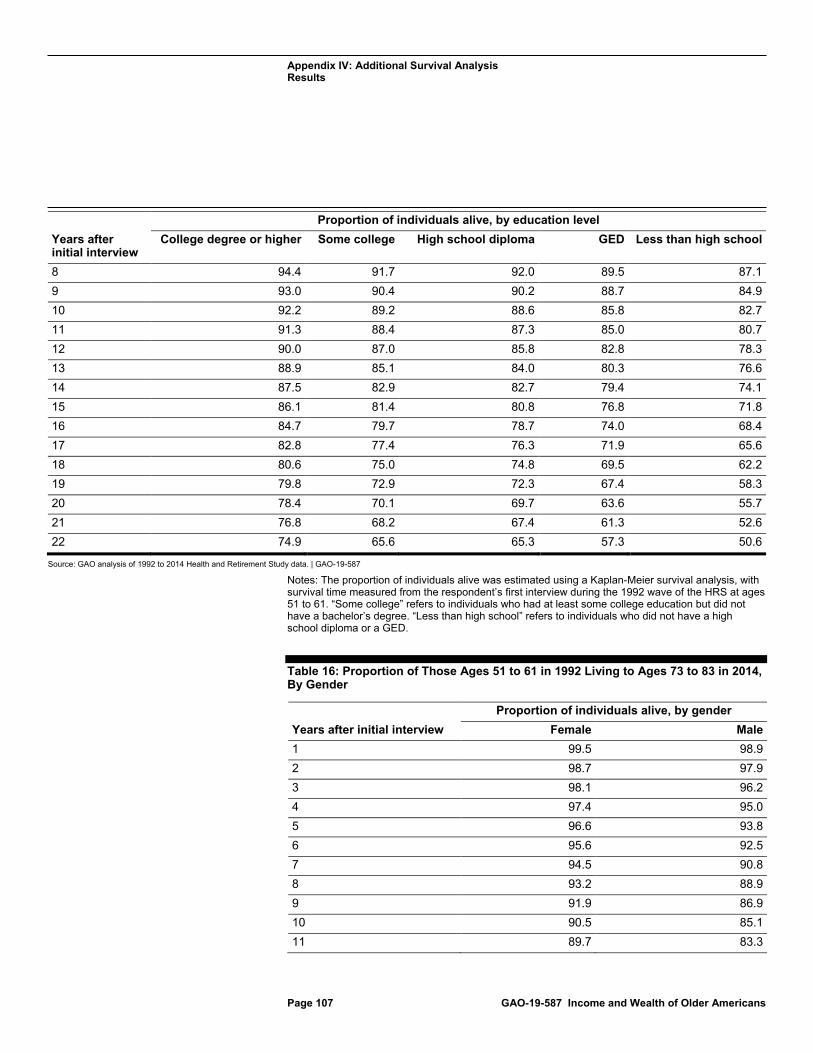
Appendix IV: Additional Survival Analysis Results
Page 107 GAO-19-587 Income and Wealth of Older Americans
Proportion of individuals alive, by education level Years after initial interview
College degree or higher Some college High school diploma GED Less than high school
8 94.4 91.7 92.0 89.5 87.1 9 93.0 90.4 90.2 88.7 84.9 10 92.2 89.2 88.6 85.8 82.7 11 91.3 88.4 87.3 85.0 80.7 12 90.0 87.0 85.8 82.8 78.3 13 88.9 85.1 84.0 80.3 76.6 14 87.5 82.9 82.7 79.4 74.1 15 86.1 81.4 80.8 76.8 71.8 16 84.7 79.7 78.7 74.0 68.4 17 82.8 77.4 76.3 71.9 65.6 18 80.6 75.0 74.8 69.5 62.2 19 79.8 72.9 72.3 67.4 58.3 20 78.4 70.1 69.7 63.6 55.7 21 76.8 68.2 67.4 61.3 52.6 22 74.9 65.6 65.3 57.3 50.6
Source: GAO analysis of 1992 to 2014 Health and Retirement Study data. | GAO-19-587
Notes: The proportion of individuals alive was estimated using a Kaplan-Meier survival analysis, with survival time measured from the respondent’s first interview during the 1992 wave of the HRS at ages 51 to 61. “Some college” refers to individuals who had at least some college education but did not have a bachelor’s degree. “Less than high school” refers to individuals who did not have a high school diploma or a GED.
Table 16: Proportion of Those Ages 51 to 61 in 1992 Living to Ages 73 to 83 in 2014, By Gender
Proportion of individuals alive, by gender Years after initial interview Female Male 1 99.5 98.9 2 98.7 97.9 3 98.1 96.2 4 97.4 95.0 5 96.6 93.8 6 95.6 92.5 7 94.5 90.8 8 93.2 88.9 9 91.9 86.9 10 90.5 85.1 11 89.7 83.3

Appendix IV: Additional Survival Analysis Results
Page 108 GAO-19-587 Income and Wealth of Older Americans
Proportion of individuals alive, by gender Years after initial interview Female Male 12 88.4 81.2 13 87.0 79.3 14 85.4 77.3 15 84.0 75.0 16 81.7 72.8 17 79.6 70.1 18 77.3 67.8 19 75.0 65.3 20 72.7 62.6 21 70.6 60.2 22 68.6 57.8
Source: GAO analysis of 1992 to 2014 Health and Retirement Study data. | GAO-19-587
Notes: The proportion of individuals alive was estimated using a Kaplan-Meier survival analysis, with survival time measured from the respondent’s first interview during the 1992 wave of the HRS at ages 51 to 61.
Table 17: Proportion of Those Ages 51 to 61 in 1992 Living to Ages 73 to 83 in 2014, By Self-Reported Health Status in 1992
Proportion of individuals alive, by self-reported health status in 1992 Years after initial interview
Excellent Very good Good Fair Poor
1 99.8 99.7 99.4 98.5 95.7 2 99.6 99.4 98.7 96.8 91.5 3 98.9 98.6 97.8 95.1 87.5 4 98.6 98.1 97.1 93.1 83.8 5 98.3 97.2 96.3 91.4 81.2 6 97.9 96.5 95.1 89.5 77.5 7 97.3 95.9 93.4 86.6 74.4 8 96.5 95.2 92.2 82.7 69.8 9 95.4 94.2 90.3 80.5 65.5 10 94.8 93.0 88.3 77.8 62.4 11 93.9 92.3 86.7 75.8 60.4 12 93.3 90.9 84.7 73.2 57.0 13 92.3 89.6 82.8 70.5 54.3 14 91.6 88.1 80.7 68.2 50.2 15 90.5 86.2 78.8 65.5 47.9 16 89.3 84.7 76.0 61.6 44.7 17 87.6 82.7 73.6 57.9 41.7
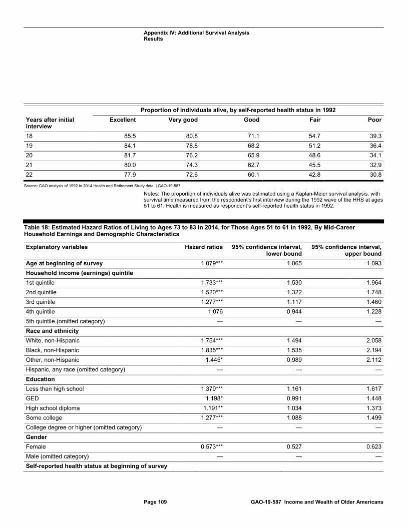
Appendix IV: Additional Survival Analysis Results
Page 109 GAO-19-587 Income and Wealth of Older Americans
Proportion of individuals alive, by self-reported health status in 1992 Years after initial interview
Excellent Very good Good Fair Poor
18 85.5 80.8 71.1 54.7 39.3 19 84.1 78.8 68.2 51.2 36.4 20 81.7 76.2 65.9 48.6 34.1 21 80.0 74.3 62.7 45.5 32.9 22 77.9 72.6 60.1 42.8 30.8
Source: GAO analysis of 1992 to 2014 Health and Retirement Study data. | GAO-19-587
Notes: The proportion of individuals alive was estimated using a Kaplan-Meier survival analysis, with survival time measured from the respondent’s first interview during the 1992 wave of the HRS at ages 51 to 61. Health is measured as respondent’s self-reported health status in 1992.
Table 18: Estimated Hazard Ratios of Living to Ages 73 to 83 in 2014, for Those Ages 51 to 61 in 1992, By Mid-Career Household Earnings and Demographic Characteristics
Explanatory variables Hazard ratios 95% confidence interval, lower bound
95% confidence interval, upper bound
Age at beginning of survey 1.079*** 1.065 1.093 Household income (earnings) quintile 1st quintile 1.733*** 1.530 1.964 2nd quintile 1.520*** 1.322 1.748 3rd quintile 1.277*** 1.117 1.460 4th quintile 1.076 0.944 1.228 5th quintile (omitted category) — — — Race and ethnicity White, non-Hispanic 1.754*** 1.494 2.058 Black, non-Hispanic 1.835*** 1.535 2.194 Other, non-Hispanic 1.445* 0.989 2.112 Hispanic, any race (omitted category) — — — Education Less than high school 1.370*** 1.161 1.617 GED 1.198* 0.991 1.448 High school diploma 1.191** 1.034 1.373 Some college 1.277*** 1.088 1.499 College degree or higher (omitted category) — — — Gender Female 0.573*** 0.527 0.623 Male (omitted category) — — — Self-reported health status at beginning of survey
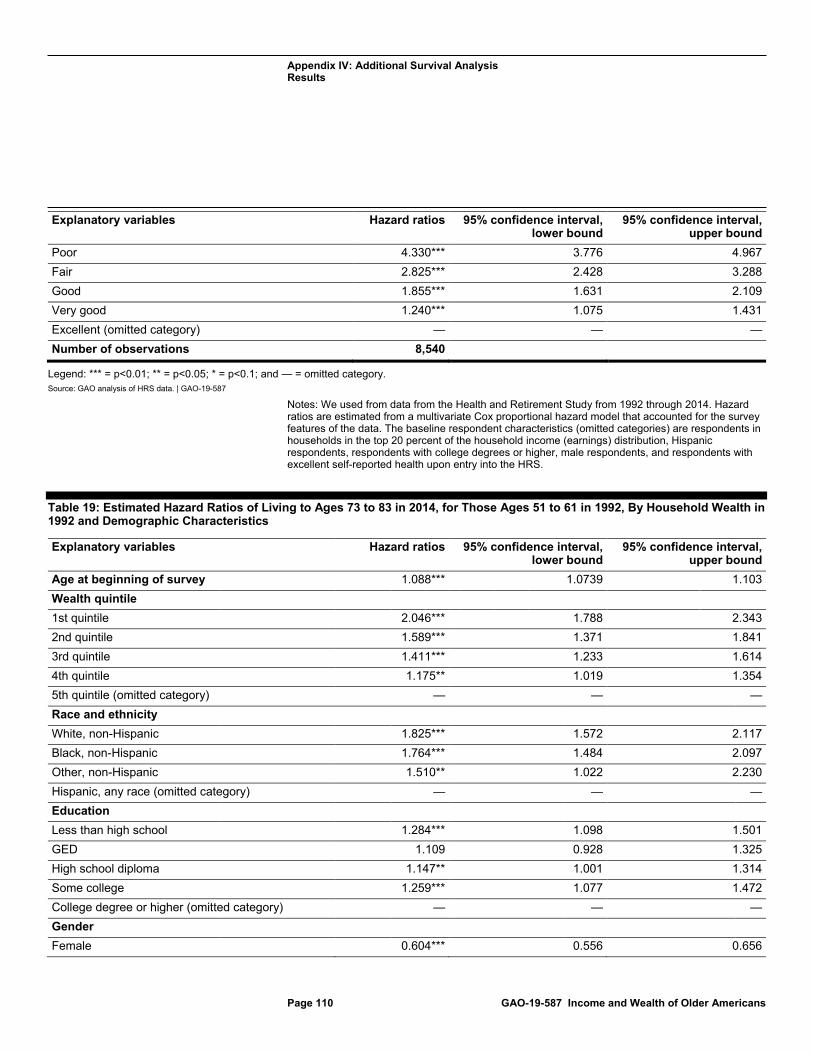
Appendix IV: Additional Survival Analysis Results
Page 110 GAO-19-587 Income and Wealth of Older Americans
Explanatory variables Hazard ratios 95% confidence interval, lower bound
95% confidence interval, upper bound
Poor 4.330*** 3.776 4.967 Fair 2.825*** 2.428 3.288 Good 1.855*** 1.631 2.109 Very good 1.240*** 1.075 1.431 Excellent (omitted category) — — — Number of observations 8,540
Legend: *** = p<0.01; ** = p<0.05; * = p<0.1; and — = omitted category. Source: GAO analysis of HRS data. | GAO-19-587
Notes: We used from data from the Health and Retirement Study from 1992 through 2014. Hazard ratios are estimated from a multivariate Cox proportional hazard model that accounted for the survey features of the data. The baseline respondent characteristics (omitted categories) are respondents in households in the top 20 percent of the household income (earnings) distribution, Hispanic respondents, respondents with college degrees or higher, male respondents, and respondents with excellent self-reported health upon entry into the HRS.
Table 19: Estimated Hazard Ratios of Living to Ages 73 to 83 in 2014, for Those Ages 51 to 61 in 1992, By Household Wealth in 1992 and Demographic Characteristics
Explanatory variables Hazard ratios 95% confidence interval, lower bound
95% confidence interval, upper bound
Age at beginning of survey 1.088*** 1.0739 1.103 Wealth quintile 1st quintile 2.046*** 1.788 2.343 2nd quintile 1.589*** 1.371 1.841 3rd quintile 1.411*** 1.233 1.614 4th quintile 1.175** 1.019 1.354 5th quintile (omitted category) — — — Race and ethnicity White, non-Hispanic 1.825*** 1.572 2.117 Black, non-Hispanic 1.764*** 1.484 2.097 Other, non-Hispanic 1.510** 1.022 2.230 Hispanic, any race (omitted category) — — — Education Less than high school 1.284*** 1.098 1.501 GED 1.109 0.928 1.325 High school diploma 1.147** 1.001 1.314 Some college 1.259*** 1.077 1.472 College degree or higher (omitted category) — — — Gender Female 0.604*** 0.556 0.656
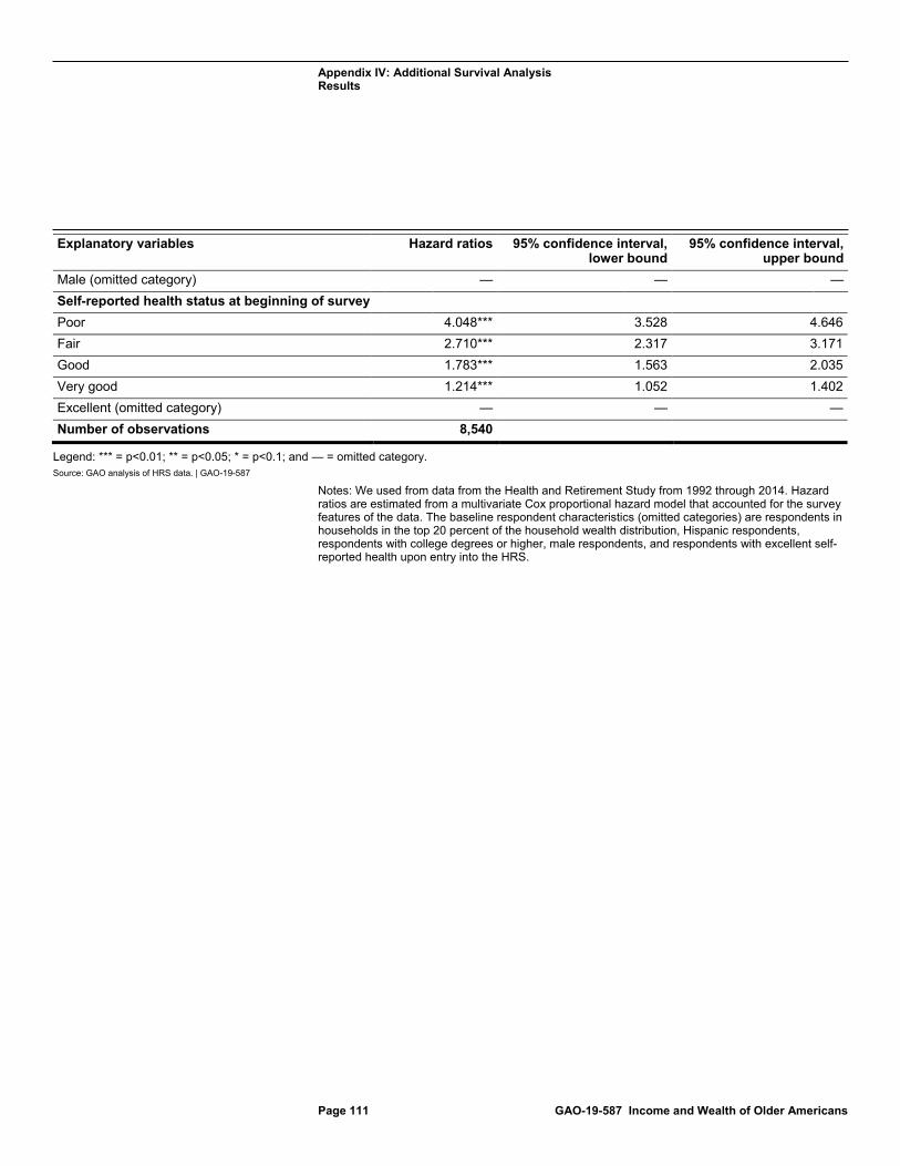
Appendix IV: Additional Survival Analysis Results
Page 111 GAO-19-587 Income and Wealth of Older Americans
Explanatory variables Hazard ratios 95% confidence interval, lower bound
95% confidence interval, upper bound
Male (omitted category) — — — Self-reported health status at beginning of survey Poor 4.048*** 3.528 4.646 Fair 2.710*** 2.317 3.171 Good 1.783*** 1.563 2.035 Very good 1.214*** 1.052 1.402 Excellent (omitted category) — — — Number of observations 8,540
Legend: *** = p<0.01; ** = p<0.05; * = p<0.1; and — = omitted category. Source: GAO analysis of HRS data. | GAO-19-587
Notes: We used from data from the Health and Retirement Study from 1992 through 2014. Hazard ratios are estimated from a multivariate Cox proportional hazard model that accounted for the survey features of the data. The baseline respondent characteristics (omitted categories) are respondents in households in the top 20 percent of the household wealth distribution, Hispanic respondents, respondents with college degrees or higher, male respondents, and respondents with excellent self-reported health upon entry into the HRS.
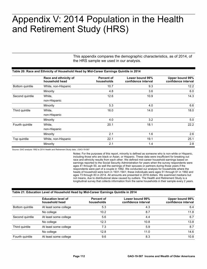
Appendix V: 2014 Population in the Health and Retirement Study (HRS)
Page 112 GAO-19-587 Income and Wealth of Older Americans
This appendix compares the demographic characteristics, as of 2014, of the HRS sample we used in our analysis.
Table 20: Race and Ethnicity of Household Head by Mid-Career Earnings Quintile in 2014
Race and ethnicity of household head
Percent of households
Lower bound 99% confidence interval
Upper bound 99% confidence interval
Bottom quintile White, non-Hispanic 10.7 9.3 12.2 Minority 4.8 3.6 6.0 Second quintile White,
non-Hispanic 12.6 10.9 14.3
Minority 5.3 4.0 6.6 Third quintile White,
non-Hispanic 16.0 14.0 18.0
Minority 4.0 3.2 5.0 Fourth quintile White,
non-Hispanic 20.1 18.1 22.2
Minority 2.1 1.6 2.6 Top quintile White, non-Hispanic 22.1 19.1 25.1 Minority 2.1 1.4 2.8
Source: GAO analysis 1992 to 2014 Health and Retirement Study data. | GAO-19-587
Notes: For the purposes of this report, minority is defined as someone who is non-white or Hispanic, including those who are black or Asian, or Hispanic. These data were insufficient for breaking out race and ethnicity results from each other. We defined mid-career household earnings based on earnings reported to the Social Security Administration for years when the survey respondents were ages 41 through 50, as well the earnings of their spouses or partners during those years if the respondents were part of a couple in 1992. We conducted our analysis for households where the heads of household were born in 1931-1941; these individuals were ages 51 through 61 in 1992 and ages 73 through 83 in 2014. All amounts are presented in 2016 dollars. We examined medians but not means, due to distributional skew caused by outliers. The Health and Retirement Study is a longitudinal survey that collects information from the same households in their sample every 2 years.
Table 21: Education Level of Household Head by Mid-Career Earnings Quintile in 2014
Education level of household head
Percent of households
Lower bound 99% confidence interval
Upper bound 99% confidence interval
Bottom quintile At least some college 5.3 4.3 6.4 No college 10.2 8.7 11.8 Second quintile At least some college 5.6 4.4 6.7 No college 12.3 10.8 13.8 Third quintile At least some college 7.3 5.9 8.7 No college 12.8 11.0 14.6 Fourth quintile At least some college 9.6 8.3 10.8
Appendix V: 2014 Population in the Health and Retirement Study (HRS)
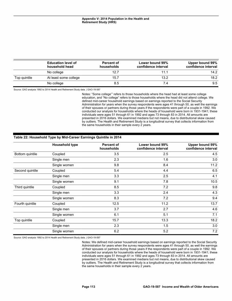
Appendix V: 2014 Population in the Health and Retirement Study (HRS)
Page 113 GAO-19-587 Income and Wealth of Older Americans
Education level of household head
Percent of households
Lower bound 99% confidence interval
Upper bound 99% confidence interval
No college 12.7 11.1 14.2 Top quintile At least some college 15.7 13.2 18.2 No college 8.5 7.4 9.5
Source: GAO analysis 1992 to 2014 Health and Retirement Study data. | GAO-19-587
Notes: “Some college’” refers to those households where the head had at least some college education, and “No college” refers to those households where the head did not attend college. We defined mid-career household earnings based on earnings reported to the Social Security Administration for years when the survey respondents were ages 41 through 50, as well the earnings of their spouses or partners during those years if the respondents were part of a couple in 1992. We conducted our analysis for households where the heads of household were born in 1931-1941; these individuals were ages 51 through 61 in 1992 and ages 73 through 83 in 2014. All amounts are presented in 2016 dollars. We examined medians but not means, due to distributional skew caused by outliers. The Health and Retirement Study is a longitudinal survey that collects information from the same households in their sample every 2 years.
Table 22: Household Type by Mid-Career Earnings Quintile in 2014
Household type Percent of households
Lower bound 99% confidence interval
Upper bound 99% confidence interval
Bottom quintile Coupled 3.5 2.5 4.5 Single men 2.3 1.6 3.0 Single women 9.8 8.4 11.2 Second quintile Coupled 5.4 4.4 6.5 Single men 3.3 2.5 4.1 Single women 9.1 7.8 10.5 Third quintile Coupled 8.5 7.2 9.8 Single men 3.3 2.4 4.3 Single women 8.3 7.2 9.4 Fourth quintile Coupled 12.5 11.2 13.7 Single men 3.7 2.7 4.6 Single women 6.1 5.1 7.1 Top quintile Coupled 15.7 13.3 18.2 Single men 2.3 1.5 3.0 Single women 6.2 5.2 7.2
Source: GAO analysis 1992 to 2014 Health and Retirement Study data. | GAO-19-587
Notes: We defined mid-career household earnings based on earnings reported to the Social Security Administration for years when the survey respondents were ages 41 through 50, as well the earnings of their spouses or partners during those years if the respondents were part of a couple in 1992. We conducted our analysis for households where the heads of household were born in 1931-1941; these individuals were ages 51 through 61 in 1992 and ages 73 through 83 in 2014. All amounts are presented in 2016 dollars. We examined medians but not means, due to distributional skew caused by outliers. The Health and Retirement Study is a longitudinal survey that collects information from the same households in their sample every 2 years.
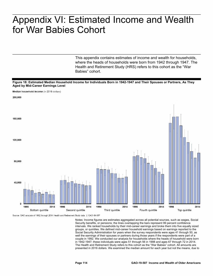
Appendix VI: Estimated Income and Wealth for War Babies Cohort
Page 114 GAO-19-587 Income and Wealth of Older Americans
This appendix contains estimates of income and wealth for households, where the heads of households were born from 1942 through 1947. The Health and Retirement Study (HRS) refers to this cohort as the “War Babies” cohort.
Figure 18: Estimated Median Household Income for Individuals Born in 1942-1947 and Their Spouses or Partners, As They Aged by Mid-Career Earnings Level
Notes: Income figures are estimates aggregated across all potential sources, such as wages, Social Security benefits, or pensions; the lines overlapping the bars represent 99 percent confidence intervals. We ranked households by their mid-career earnings and broke them into five equally sized groups, or quintiles. We defined mid-career household earnings based on earnings reported to the Social Security Administration for years when the survey respondents were ages 41 through 50, as well the earnings of their spouses or partners during those years if the respondents were part of a couple in 1992. We conducted our analysis for households where the heads of household were born in 1942-1947; these individuals were ages 51 through 56 in 1998 and ages 67 through 72 in 2014. The Health and Retirement Study refers to this cohort as the “War Babies” cohort. All amounts are presented in 2016 dollars. We examined the median amount for each year but not the means, due to
Appendix VI: Estimated Income and Wealth for War Babies Cohort
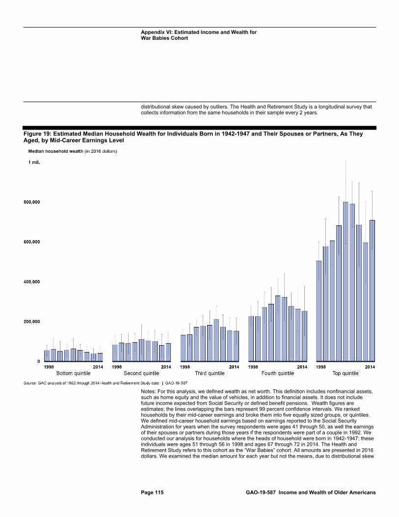
Appendix VI: Estimated Income and Wealth for War Babies Cohort
Page 115 GAO-19-587 Income and Wealth of Older Americans
distributional skew caused by outliers. The Health and Retirement Study is a longitudinal survey that collects information from the same households in their sample every 2 years.
Figure 19: Estimated Median Household Wealth for Individuals Born in 1942-1947 and Their Spouses or Partners, As They Aged, by Mid-Career Earnings Level
Notes: For this analysis, we defined wealth as net worth. This definition includes nonfinancial assets, such as home equity and the value of vehicles, in addition to financial assets. It does not include future income expected from Social Security or defined benefit pensions. Wealth figures are estimates; the lines overlapping the bars represent 99 percent confidence intervals. We ranked households by their mid-career earnings and broke them into five equally sized groups, or quintiles. We defined mid-career household earnings based on earnings reported to the Social Security Administration for years when the survey respondents were ages 41 through 50, as well the earnings of their spouses or partners during those years if the respondents were part of a couple in 1992. We conducted our analysis for households where the heads of household were born in 1942-1947; these individuals were ages 51 through 56 in 1998 and ages 67 through 72 in 2014. The Health and Retirement Study refers to this cohort as the “War Babies” cohort. All amounts are presented in 2016 dollars. We examined the median amount for each year but not the means, due to distributional skew

Appendix VI: Estimated Income and Wealth for War Babies Cohort
Page 116 GAO-19-587 Income and Wealth of Older Americans
caused by outliers. The Health and Retirement Study is a longitudinal survey that collects information from the same households in their sample every 2 years.
Appendix VII: GAO Contact and Staff Acknowledgments
Page 117 GAO-19-587 Income and Wealth of Older Americans
Charles A. Jeszeck, (202) 512-7215, [email protected]
In addition to the contact named above, Michael Collins (Assistant Director), Jennifer Gregory (Analyst-in-Charge), Garrick Donnelly, Kathleen McQueeney, Chris Wickham, and Christopher Zbrozek made key contributions to this report. Also contributing to this report were Susan Aschoff, James Bennett, Deborah Bland, Melinda Bowman, Nisha Hazra, Kirsten Lauber, Jeffrey Miller, Oliver Richard, Amrita Sen, Joseph Silvestri, Jeff Tessin, Frank Todisco, Adam Wendel, and Sirin Yaemsiri.
Appendix VII: GAO Contact and Staff Acknowledgments
GAO Contact
Staff Acknowledgments
Bibliography
Page 118 GAO-19-587 Income and Wealth of Older Americans
Auerbach, Alan J., Laurence J. Kotlikoff, and Darryl R. Koehler. “U.S. Inequality, Fiscal Progressivity, and Work Disincentives: An Intragenerational Accounting.” NBER Working Paper, no. 22032 (2016).
Banerjee, Sudipto. “Asset Decumulation or Asset Preservation? What Guides Retirement Spending?” EBRI Issue Brief, no. 447 (2018).
Banerjee, Sudipto. “Income Composition, Income Trends and Income Shortfalls of Older Households.” EBRI Issue Brief, no. 383 (2013).
Bee, Adam and Joshua Mitchell. “Do Older Americans Have More Income Than We Think?” SESHD Working Paper, vol. 2017, no. 39 (2017).
Board of Governors of the Federal Reserve System. “Changes in U.S. Family Finances from 2013 to 2016: Evidence from the Survey of Consumer Finances,” Federal Reserve Bulletin, vol. 103, no. 3 (Washington, D.C.: September 2017).
Bosworth, Barry P. and Kan Zhang. “Evidence of Increasing Differential Mortality: A Comparison of the HRS and SIPP.” Center for Retirement Research Working Paper, vol. 2015, no. 13 (2015).
Bricker, Jesse, Alice M. Henriques, Jake A. Krimmel, and John E. Sabelhaus. “Measuring Income and Wealth at the Top Using Administrative and Survey Data.” Finance and Economics Discussion Series, vol. 2015, no. 030 (2015).
Brookings Economic Studies Program. Later Retirement, Inequality in Old Age, and the Growing Gap in Longevity between Rich and Poor (Washington, D.C.: Brookings Institution, 2016).
Burtless, Gary. “What Do Stock Market Fluctuations Mean for the Economy?” Brookings Opinions, February 23, 2018. Accessed March 14, 2019, https://www.brookings.edu/opinions/what-do-stock-market-fluctuations-mean-for-the-economy?/
Chen, Anqi, Alicia H. Munnell, and Geoffrey T. Sanzenbacher. “How Much Income Do Retirees Actually Have? Evaluating the Evidence from Five National Datasets.” Center for Retirement Research Working Paper, vol. 2018, no. 14 (2018).
Chetty, Raj, Michael Stepner, Sarah Abraham, Shelby Lin, Benjamin Scuderi, Nicholas Turner, Augustin Bergeron, and David Cutler. “The
Bibliography
Bibliography
Page 119 GAO-19-587 Income and Wealth of Older Americans
Association Between Income and Life Expectancy in the United States, 2001-2014.” JAMA, vol. 315, no. 16 (2016).
Choi, HwaJung and Robert F. Schoeni. “Health of Americans Who Must Work Longer to Reach Social Security Retirement Age.” Health Affairs, vol. 36, no. 10 (2017).
Congressional Budget Office. Measuring the Adequacy of Retirement Income: A Primer. 53191. Washington, D.C.: October 2017.
Congressional Budget Office. Trends in Family Wealth, 1989 to 2013. 51846. Washington, D.C.: August 2016.
Congressional Research Service. The U.S. Income Distribution: Trends and Issues. R44705. Washington, D.C.: December 8, 2016.
Devlin-Foltz, Sebastian, Alice Henriques, and John Sabelhous. “Is the U.S. Retirement System Contributing to Rising Wealth Inequality?” The Russell Sage Foundation Journal of the Social Sciences, vol. 2, no. 6 (2016).
Federal Reserve Bank of St. Louis. “When the Stock Market Rises, Who Benefits?” On the Economy Blog, February 27, 2018. Accessed March 14, 2019, https://www.stlouisfed.org/on-the-economy/2018/february/when-stock-market-rises-who-benefits.
Ghilarducci, Teresa, Siavash Radpour, and Anthony Webb. “Employer Retirement Wealth Inequality: 1992 and 2010.” Paper presented at the annual meeting of the American Economics Association Meetings, Philadelphia, P.A.: January 6, 2018.
Goda, Gopi Shah, Shanthi Ramnath, John B. Shoven, and Sita Nataraj Slavov. “The Financial Feasibility of Delaying Social Security: Evidence from Administrative Tax Data.” Journal of Pension Economics and Finance, vol. 17, no. 4 (2018).
Gustman, Alan, Thomas Steinmeier, and Nahid Tabatabai. “Distributional Effects of Means Testing Social Security: Income Versus Wealth.” NBER Working Paper Series, no. 22424 (2016).
Johnson, Barry W. and Brian Raub. “How Much Longevity Can Money Buy? Estimating Mortality Rates for Wealthy Individuals.” Statistical Journal of the IAOS, vol. 34 (2018).
Bibliography
Page 120 GAO-19-587 Income and Wealth of Older Americans
Johnson, Richard W. Delayed Retirement and the Growth in Income Inequality at Older Ages (Washington, D.C.: Urban Institute, 2018).
Kindig, David A. and Erika R. Cheng. “Even As Mortality Fell in Most US Counties, Female Mortality Nonetheless Rose in 42.8 Percent of Counties From 1992 to 2006.” Health Affairs, vol. 32, no. 3 (2013).
Olshansky, S. Jay, Toni Antonucci, Lisa Berkman, Robert H. Binstock, Axel Boersch-Supan, John T. Cacioppo, Bruce A. Carnes, Laura L. Carstensen, Linda P. Fried, Dana P. Goldman, James Jackson, Martin Kohli, John Rother, Yuhui Zheng, and John Rowe. “Differences in Life Expectancy Due to Race and Educational Differences Are Widening, and Many May Not Catch Up.” Health Affairs, vol. 31, no. 8 (2012).
Owyang, Michael T. and Hannah G. Shell. “Taking Stock: Income Inequality and the Stock Market.” Economic Synopses, No. 7 (2016).
Pijoan-Mas, Josep and Jose-Victor Rios-Rull. “Heterogeneity in Expected Longevities.” Demography, vol. 51, no. 6 (2014).
Poterba, James M. “Retirement Security in an Aging Population.” The American Economic Review, vol. 104, no. 5 (2014).
Poterba, James, Steven Venti, and David A. Wise. “Longitudinal Determinants of End-of-Life Wealth Inequality.” Journal of Public Economics, vol. 162 (2018).
Poterba, James M., Steven F. Venti, and David A. Wise. “Were They Prepared for Retirement? Financial Status at Advanced Ages in the HRS and AHEAD Cohorts.” NBER Working Papers, no. 17824 (2012).
Poterba, James, Steven Venti, and David Wise. “The Composition and Drawdown of Wealth in Retirement.” Journal of Economic Perspectives, vol. 25, no. 4 (2011).
Raskin, Sarah Bloom. “Downturns and Recoveries: What the Economies in Los Angeles and the United States Tell Us.” Remarks at the luncheon for Los Angeles business and community leaders, Los Angeles Branch of the Federal Reserve Bank of San Francisco. April 12, 2012.
Ruiz, John M., Patrick Steffen, and Timothy B. Smith. “Hispanic Mortality Paradox: A Systematic Review and Meta-Analysis of the Longitudinal
Bibliography
Page 121 GAO-19-587 Income and Wealth of Older Americans
Literature.” American Journal of Public Health, vol. 103, no. 3 (February 2012).
Saez, Emmanuel and Gabriel Zucman. “Wealth Inequality in the United States Since 1913: Evidence from Capitalized Income Tax Data.” The Quarterly Journal of Economics, vol. 131, no. 2 (2016).
Waldron, Hilary. “Mortality Differentials by Lifetime Earnings Decile: Implications for Evaluations of Proposed Social Security Law Changes.” Social Security Bulletin, vol. 73, no. 1 (2013).
Waldron, Hilary. “Trends in Mortality Differentials and Life Expectancy for Male Social Security-Covered Workers, by Socioeconomic Status.” Social Security Bulletin, vol. 67, no. 3 (2007).
Wang, Haidong, Austin E Schumacher, Carly E Levitz, Ali H Mokdad, and Christopher JL Murray. “Left Behind: Widening Disparities for Males and Females in US County Life Expectancy, 1985-2010.” Population Health Metrics, vol. 11, no. 8 (2013).
Related GAO Products
Page 122 GAO-19-587 Income and Wealth of Older Americans
Retirement Security: Most Households Approaching Retirement Have Low Savings, an Update. GAO-19-442R. Washington, D.C.: Mar. 26, 2019.
The Nation’s Retirement System: A Comprehensive Re-evaluation Needed to Better Promote Future Retirement Security. GAO-19-342T. Washington, D.C.: Feb. 6, 2019.
The Nation’s Retirement System: A Comprehensive Re-evaluation Is Needed to Better Promote Future Retirement Security. GAO-18-111SP. Washington, D.C.: Oct.18, 2017.
Older Workers: Phased Retirement Programs, Although Uncommon, Provide Flexibility for Workers and Employers. GAO-17-536. Washington, D.C.: June 20, 2017.
Retirement Security: Low Defined Contribution Savings May Pose Challenges. GAO-16-408. Washington, D.C.: May 5, 2016.
Retirement Security: Shorter Life Expectancy Reduces Projected Lifetime Benefits for Lower Earners. GAO-16-354. Washington, D.C.: Mar. 25, 2016.
Retirement Security: Better Information on Income Replacement Rates Needed to Help Workers Plan for Retirement. GAO-16-242. Washington, D.C.: Mar. 1, 2016.
Retirement Security: Most Households Approaching Retirement Have Low Savings. GAO-15-419. Washington, D.C.: May 12, 2015.
Retirement Security: Trends in Marriage and Work Patterns May Increase Economic Vulnerability for Some Retirees. GAO-14-33. Washington, D.C.: Jan. 15, 2014.
Retirement Security: Women Still Face Challenges. GAO-12-699. Washington, D.C.: July 19, 2012.
Unemployed Older Workers: Many Experience Challenges Regaining Employment and Face Reduced Retirement Security. GAO-12-445. Washington, D.C.: Apr. 25, 2012.
Related GAO Products
(102142)
The Government Accountability Office, the audit, evaluation, and investigative arm of Congress, exists to support Congress in meeting its constitutional responsibilities and to help improve the performance and accountability of the federal government for the American people. GAO examines the use of public funds; evaluates federal programs and policies; and provides analyses, recommendations, and other assistance to help Congress make informed oversight, policy, and funding decisions. GAO’s commitment to good government is reflected in its core values of accountability, integrity, and reliability.
The fastest and easiest way to obtain copies of GAO documents at no cost is through GAO’s website (https://www.gao.gov). Each weekday afternoon, GAO posts on its website newly released reports, testimony, and correspondence. To have GAO e-mail you a list of newly posted products, go to https://www.gao.gov and select “E-mail Updates.”
The price of each GAO publication reflects GAO’s actual cost of production and distribution and depends on the number of pages in the publication and whether the publication is printed in color or black and white. Pricing and ordering information is posted on GAO’s website, https://www.gao.gov/ordering.htm.
Place orders by calling (202) 512-6000, toll free (866) 801-7077, or TDD (202) 512-2537.
Orders may be paid for using American Express, Discover Card, MasterCard, Visa, check, or money order. Call for additional information.
Connect with GAO on Facebook, Flickr, Twitter, and YouTube. Subscribe to our RSS Feeds or E-mail Updates. Listen to our Podcasts. Visit GAO on the web at https://www.gao.gov.
Contact FraudNet:
Website: https://www.gao.gov/fraudnet/fraudnet.htm
Automated answering system: (800) 424-5454 or (202) 512-7700
Orice Williams Brown, Managing Director, [email protected], (202) 512-4400, U.S. Government Accountability Office, 441 G Street NW, Room 7125, Washington, DC 20548
Chuck Young, Managing Director, [email protected], (202) 512-4800 U.S. Government Accountability Office, 441 G Street NW, Room 7149 Washington, DC 20548
James-Christian Blockwood, Managing Director, [email protected], (202) 512-4707 U.S. Government Accountability Office, 441 G Street NW, Room 7814, Washington, DC 20548
GAO’s Mission
Obtaining Copies of GAO Reports and Testimony Order by Phone
Connect with GAO
To Report Fraud, Waste, and Abuse in Federal Programs
Congressional Relations
Public Affairs
Strategic Planning and External Liaison
Please Print on Recycled Paper.