Embed Size (px)
Citation preview
AN ABSTRACT OF THE THESIS OF
Kenneth Malcolm Glibert for the Ph. D. in Physics (Name) (Degree) (Major)
Date thesis is presented °sove,mber 16, 196,
Title GAMMA- AND BETA -RAY SPECTROSCOPY STUDIES OF THE
RADIOACTIVE DECAY OF Mn -51 TO Cr -51
Abstract approved
The decay scheme of Mn51 has been investigated using gamma-
ray and beta -ray scintillation spectrometers and a fast coincidence
spectrometer. A half -life value of 46. 5 * O. 2 minutes was deter-
mined for Mn51 which decays predominantly to the ground state of
Cr51 by the emission of positons with an experimentally measured
end -point energy of 2.. 21 ± 0. 02 MeV. Weak branching to the 761-
keV and 1170 -keV levels of Cr51, however, has been inferred from
the measured 761 ± 11 -keV and 1170 ± 15 -keV gamma -ray energies
observed in the Mn51 gamma -ray spectrum. Relative intensities for
these weak gamma -rays have been determined experimentally as
O. 70 ± O. 10 and O. 48 f 0. 12 percent of the positons, respectively.
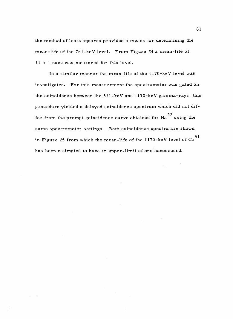
An 11 ± 1 nsec mean -life has been obtained for the 761 -keV level of
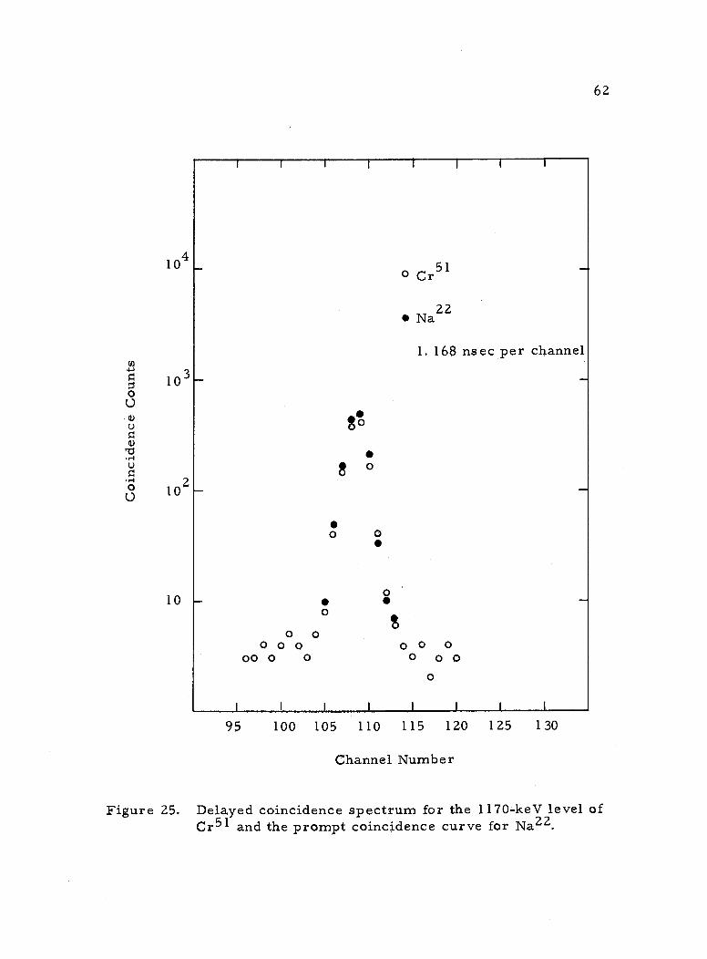
Cr51 while an upper -limit of 1 nsec has been given to the 1170 -keV
level. Using these experimental results coupled with theory, a spin
and parity assignment of 2
was given to the ground state of Mn51,
professor

a spin assignment which is not in agreement with the 7- value ex-
pected from the shell model prediction.
2
GAMMA- AND BETA -RAY SPECTROSCOPY STUDIES OF THE RADIOACTIVE DECAY OF Mn -51 TO Cr -51
by
KENNETH MALCOLM GLIBERT
A THESIS
submitted to
OREGON STATE UNIVERSITY
in partial fulfillment of the requirements for the
degree of
DOCTOR OF PHILOSOPHY
June 1966
APPROVED:
Associate professor of Physic
In Charge of Major
Act C .airm of the Department of Physics
Dean of the Graduate School
Date thesis is presented November 16, giF
Typed by Marion F. Palmateer
ACKNOWLEDGMENTS
This author wishes to take this opportunity to express his
gratitude to the following individuals whose kind and generous as-
sistance made this investigation possible: (1) Dr. H. T. Easterday,
research director and major professor, for proposing the problem
and for the many enlightening discussions pertaining to all aspects
of this investigation, (2) Dr. E. A. Yunker for his continued en-
couragement and support of the project, (3) Dr. R. W. Sommerfeldt
for his assistance in measuring the mean -life times of the first two
excited levels of Cr51, (4) Mr. Thomas L. Yates and the staff of the
Oregon State University Computing Laboratory and Mr. William
Anderson and the staff of Western Data Processing Center, Uni-
versity of California, Los Angeles, California, for their assistance
in the data analysis, (5) Mr. Jack McKenzie of the staff of the Oregon
State University cyclotron for his help in producing the Mn51 isotope,
and (6) Mr. Dale Weeden of the Oregon State University Physics
Electronics shop for designing and constructing the dwell advance
timer used in the half -life measurement and his conscientious atten-
tion to maintaining the electronic apparatus.
TABLE OF CONTENTS
INTRODUCTION
HALF -LIFE MEASUREMENT
Page
1
11
Source Production 11
Apparatus 11
Experimental Results 15
GAMMA -RAY ENERGY MEASUREMENT 18
Apparatus Experiment and Results
GAMMA -RAY RELATIVE INTENSITY MEASUREMENT
Apparatus Experiment and Results
END -POINT ENERGY MEASUREMENT
Apparatus Experiment and Results
18 18
26
26 26
40
40 43
MEAN -LIFE TIMES OF THE 761 -keV AND 1170 -keV LEVELS OF Cr -51 59
Apparatus 59
Experiment and Results 59
CONCLUSIONS 63
BIBLIOGRAPHY 84
APPENDICES 88
Appendix I Source Preparation 88 Appendix II Weighted Least Squares Fit Program 90 Appendix ITT Polynomial Curve Fitting 99 Appendix IV Backscatter Correction and Kurie Function
Calculation 108
-
LIST OF FIGURES
Figure Page
1
2
3
4
Decay scheme of Mn51 and the low -lying levels of Cr51 as summarized in the Nuclear Data Sheets. 9
Block diagram of a gamma -ray scintillation spectro- meter. 1 3
Source- detector geometry for half -life analysis and gamma -ray energy measurement. 14
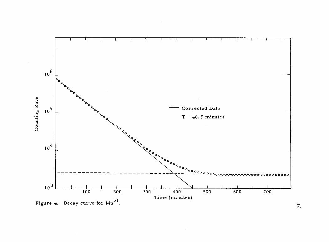
Decay curve for Mn51. 16
5 Gamma -ray pulse- height spectra for energy calibration sources. 19
Energy calibration for gamma -ray pulse- height spectra. 21
7 Gamma -ray pulse- height spectrum for Mn51 22
8 Gamma -ray spectrum for Cs l 37 28
9 Peak -to -total ratios for a 7. 6 x 7. 6 cm NaI(T1) crystal with a 10 cm source -to- detector distance. 29
10 Mn51 gamma -ray spectrum. 31
11 Y90 Bremsstrahlung distribution. 33
12 Gamma -ray spectra for Cs 1 37, Cr51, Mn54, and Zn65
sources. 34
1 3 Na22 gamma -ray spectrum. 35
14 Coincidence sum -spectrum for 511 -keV annihilation radiation. 37
15 Block diagram of a beta -gamma coincidence spectro- meter. 41
6
-
Figure Page
16 Beta -ray spectra for Cs 1 37 and Bi207 and energy
calibrat ion. 44
17 Beta -ray coincidence spectrum for Cs 1 37 K- conversion
electrons and the fit of the response function R(E, E') 45
18 Beta -ray coincidence spectrum for Bi207 -keV conversion electrons and the fit or the response function R(E, Et). 48
19 Beta -ray coincidence spectrum for Bi207 499 -keV conversion electrons and the fit of the response function R(E, Et). 49
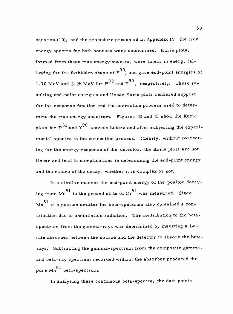
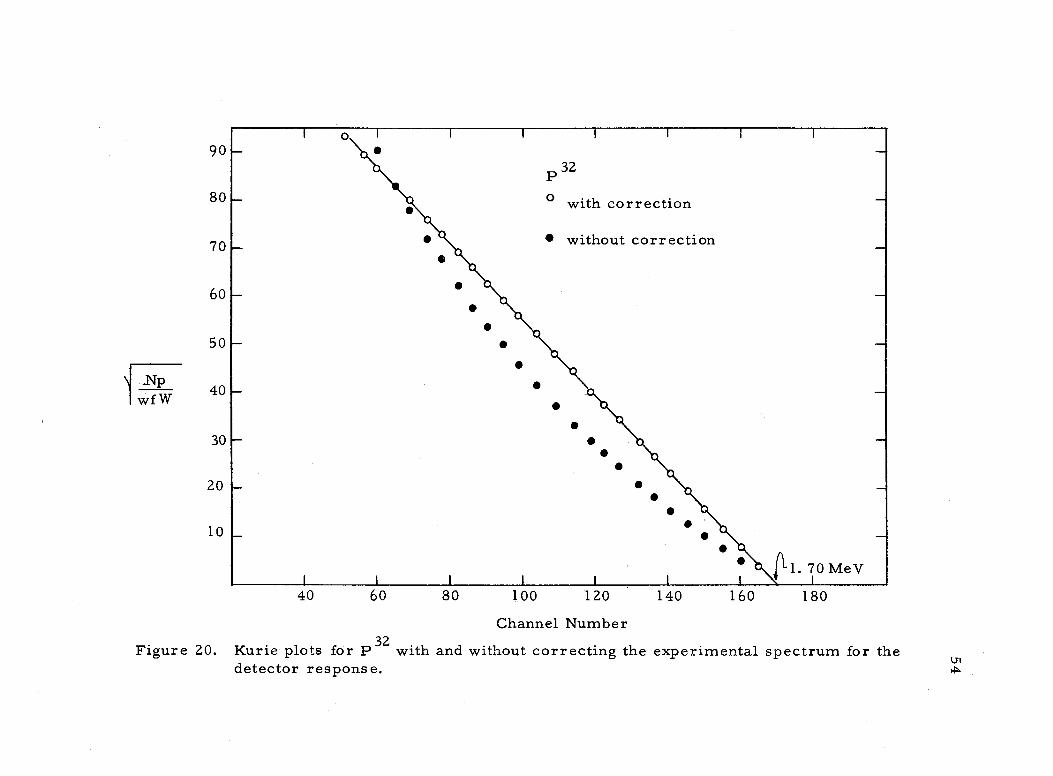
20 Kurie plots for P32 with and without correcting the experimental spectrum for the detector response. 54
21 Kurie plots for Y90 with and without correcting the experimental spectrum for the detector response. 55
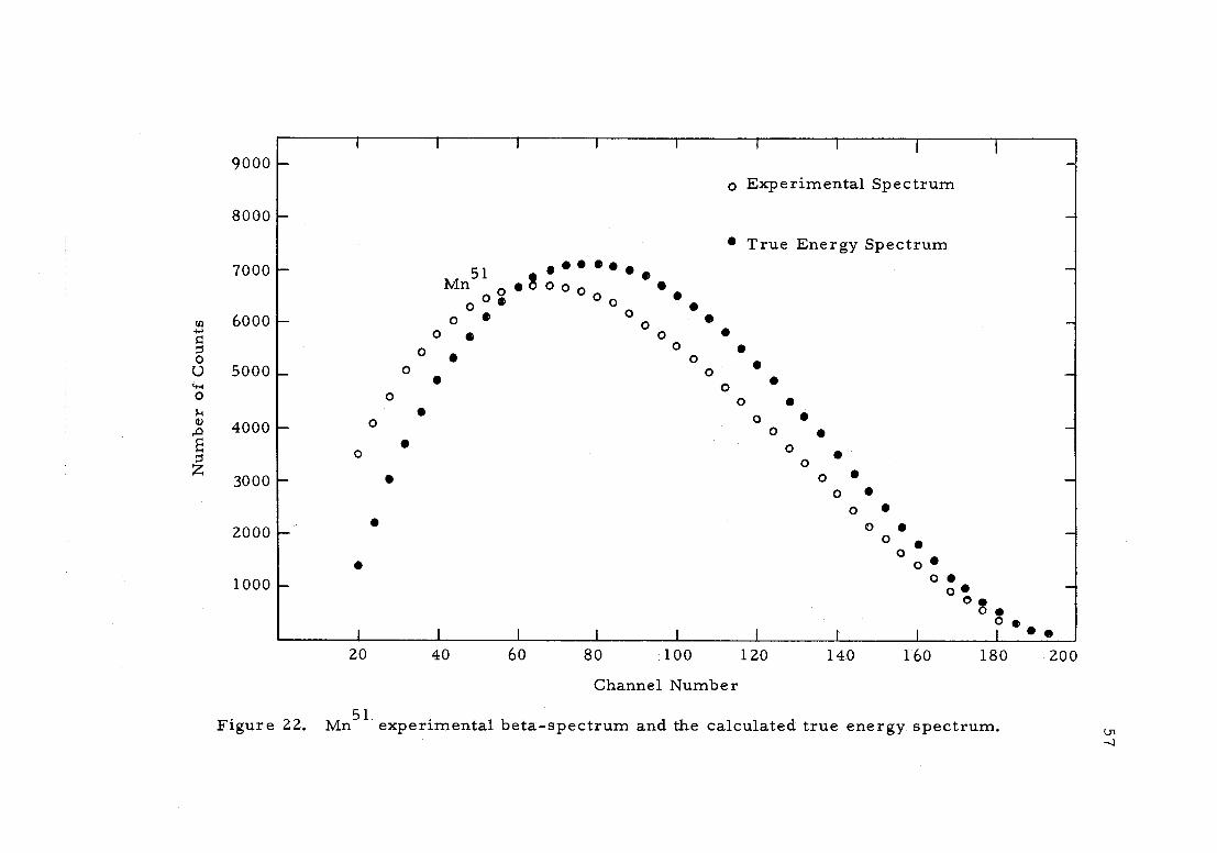
22 Mn51 experimental beta -spectrum and the calculated true energy spectrum. 57
23 Mn51 Kurie plot and energy calibration curve. 58
24 Delayed coincidence spectrum for the 761 -keV level of Cr51 and the prompt coincidence curve for Na22. 60
25 Delayed coincidence spectrum for the 1170 -key level of Cr51 and the prompt coincidence curve for Na22. 62
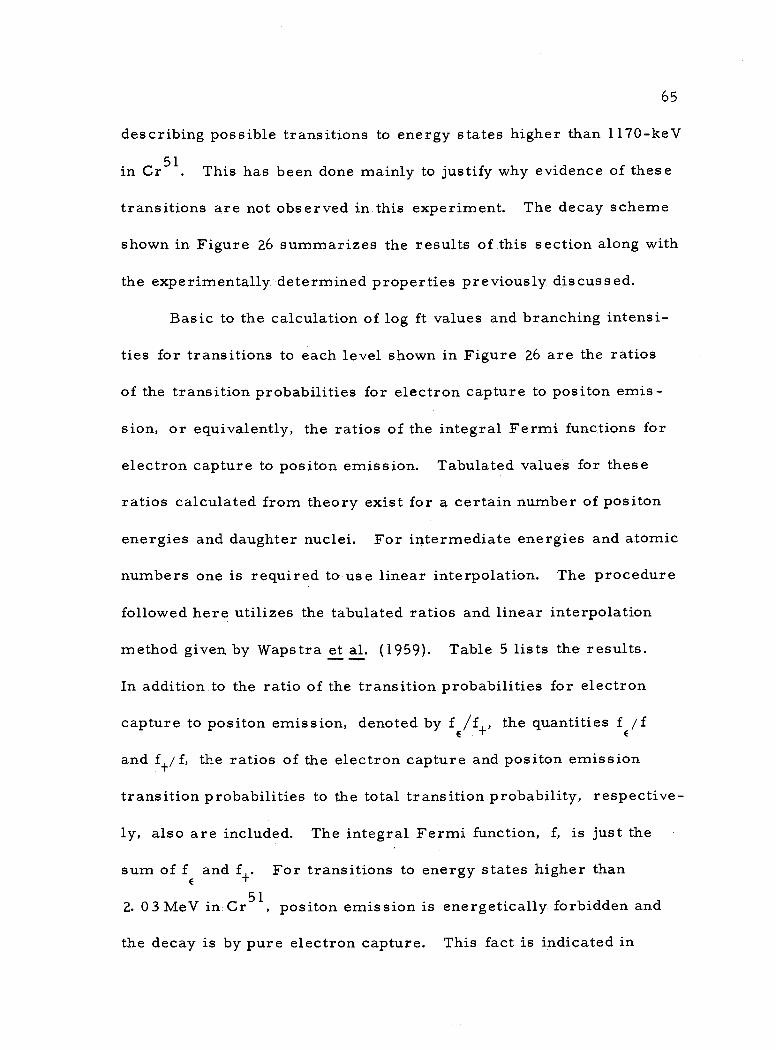
26 Decay scheme for Mn51 (present investigation). 66
27 Shell model nuclear level structure with spin -orbit coupling. 75
28 Comparison of experimentally determined half -lives for Mn51. 81
991
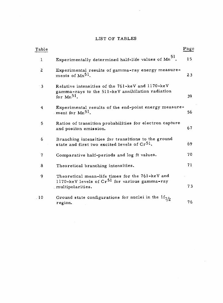
LIST OF TABLES
Table Page
1 Experimentally determined half -life values of Mn51. 15
2 Experimental results of gamma -ray energy measure- ments of Mn51. 23
3 Relative intensities of the 761 -keV and 1170 -keV gamma -rays to the 511 -keV annihilation radiation for Mn51. 39
4 Experimental results of the end -point energy measure- ment for Mn51. 56
5 Ratios of transition probabilities for electron capture and positon emission. 67
6 Branching intensities for transitions to the ground state and first two excited levels of Cr51. 69
7 Comparative half -periods and log ft values. 70
8 Theoretical branching intensities. 71
9 Theoretical mean -life times for the 761 -keV and 1170 -keV levels of Cr51 for various gamma -ray multipolarities. 73
10 Ground state configurations for nuclei in the 1f7/2 region. 76
GAMMA- AND BETA -RAY SPECTROSCOPY STUDIES OF THE RADIOACTIVE DECAY OF Mn -51 TO Cr -51
INTRODUCTION
As the theory of nuclear level structure becomes increasingly
refined, more precise and extensive knowledge concerning individual
nuclei becomes necessary. The recent improvements in the experi-
mental techniques used in low energy nuclear spectroscopy have pro-
vided means for examining nuclear properties with greater accuracy
and for extending the number of nuclei available for investigation.
In particular, the development of the multichannel analyzer has made
feasible the investigation of the level structure of short -lived iso-
topes, whereas previously, scanning experiments were restricted
to longer lived nuclei. As a result, a considerable amount of ex-
perimental information concerning the properties of low -lying nu-
clear levels has been accumulated in recent years. This informa-
tion of course is utilized by the theoretician in refining existing nu-
clear models or in formulating new theories.
The atomic nucleus which consists of various discrete energy
states is described by a set of nuclear properties. Some of these
which characterize the nucleus are the half -life, the angular mo-
mentum of the ground state and excited levels, the magnetic dipole
moment, the electric quadrupole moment, the relative parity, and
the energy and character of the nuclear transitions. Experimental
low energy nuclear physics concerns itself with investigating and
measuring these nuclear properties.
The vast amount of experimental information which has been
gathered in recent years has been subjected to the test of several
nuclear models. These models have been formulated in the absence
of a complete understanding of the exact nature of the nuclear force
existing between the nucleons within a nucleus. They are used to
correlate the experimentally determined properties and hopefully
can predict previously unknown nuclear parameters. One such
model is the nuclear shell model which was conceived independently
by Mayer, and by Haxel, Jensen, and Suess. This model is based
on the assumption that the nucleons move independently in an aver-
age central potential V(r) and furthermore are subjected to a strong a inverted spin -orbit interaction proportional to S L (Mayer and
Jensen, 1955). Strong means that this interaction is an order of
magnitude larger than that expected from the analogous spin -orbit
interaction calculation for an electron (Eisberg, 1961) where the
electron mass is replaced by the nucleon mass and the potential
energy function is the total nuclear potential V(r). Inverted spin -
orbit interaction means that the nuclear energy is decreased when
S L is positive and is increased when it is negative in contrast to
the opposite situation for the electron interaction energy. The shell
3
model was formulated originally to explain the magic numbers and
their consequences. In addition, however, it is able to explain the
spin angular momentum of the ground state of almost all odd A nuclei.
The investigation of the decay of Mn51 was performed as an addi-
tional test of the nuclear shell model in which hopefully the model
could explain the spin and parity of the ground state of Mn51 and
those of the low -lying levels of Cr51.
In the following paragraphs a chronological review is given of
the investigations on the decay of Mn51.
Livingood, Fairbrother, and Seaborg (19 37) as a result of
bombarding chromium oxides with 5. 5 -MeV deuterons were the first
to observe a manganese isotope which emitted positons with a 46
minute half -life. The isotope was positively identified as manga-
nese from chemical analysis, but the assignment of the 46 minute
activity to Mn51 was not made definite until the following year.
Livingood and Seaborg (1938) pursued the investigation still
farther by again bombarding chromium oxides or chrome plated
copper targets with a five microampere beam of 5. 5 -MeV deuterons.
Bombardment times were limited to three minutes. The activity of
the manganese which was precipitated from the irradiated target by
a radiochemical process was followed with a quartz fiber electro-
scope. An average half -life of 46 ± 2 minutes from several deter-
minations was reported.
4
In addition, the range of the positon emitted by the manganese
in aluminum was measured to be 0. 9 gram/cm2 of Al which corre-
sponds to a maximum energy of 2. 0 MeV. The gamma -ray present
was absorbed to half -value by 5. 0 grams /cm2 of Pb which is con-
sistent with the 511 -keV annihilation radiation expected in positon
decay. The presence of the 511 -keV gamma -rays strongly supported
the idea that the manganese isotope decayed by positon emission
rather than electron emission.
The assignment of the 46 minute half -life to Mn51 was estab-
lished from the following arguments given by Livingood and Seaborg.
The reaction Cr(d, n)Mn could produce the three isotopes Mn51,
Mn53, or Mn54 since natural chromium is composed of the Cr50,
Cr 52, Cr53, and Cr54 isotopes. If Mn54 is responsible for the
activity, then this same activity should be present following the deu-
teron bombardment of Fe56 through the Fe56 (d, a)Mn54 reaction.
However, the latter did not show a 46 minute activity following the
bombardment. Furthermore, the bombardment of natural manga-
nese with fast neutrons should produce the activity as a result of
the Mn55(n, 2n)Mn54 reaction, but this too failed to reveal the short-
lived activity. The Mn53 53 isotope can be eliminated on the basis of
the decay of Fe5 3. Radioactive Fe5 3 decays to Mn5 3 with a half-
life of nine minutes, and ultimately then, the 46 minute activity
would appear. However, this has been shown not to occur by
5
examining the Cr 50(a, n)Fe53 and Fe54(n, 2n)Fe53 reactions. The
possible assignment of the 46 minute activity to Mn50 which could be
produced by the Cr50(d, 2n)Mn50 reaction was rejected by studying
the excitation function for the proton reactions Cr50(p, y)Mn51 and
50 Cr (p, n)Mn . The latter of course has a sharp threshold and did
not yield the activity of 46 minutes. On the basis of these arguments,
Livingood and Seaborg concluded that the 46 minute activity must be
assigned to the Mn51 isotope.
An additional half -life measurement was performed on Mn51
by Miller, Thompson, and Cunningham (1948). They obtained a value
of 45 minutes from one bombardment only using a thin window
Geiger- Múller counter. No error was listed with their result.
Two years later, Burgus and Kennedy (1950) examined the de-
cay of Mn51 which also was produced from the Cr50(d, n) reaction by
bombarding metallic chromium with deuterons. The Mn51 was pre-
cipitated from the target which had been exposed for 1. 5 hours to a
beam current of 1 20 A. A half -life of 44. 3± 0. 5 minutes resulted
from a measurement which extended over eight half -lives using a
Geiger counter with a thin mica end -window.
The importance of the investigation of Burgus and Kennedy,
however, was not the measurement of the half -life, but was the
establishment of the genetic relationship between Mn51 and Cr 51.
Prior to this time it was known that Mn51 decayed by the emission
50
of a beta -ray and it was assumed on the basis of the observed 511 -
keV radiation that the decay was by positon emission. However, posi-
tive identification had not been made. In their experiment Burgus
and Kennedy prepared a sample of Mn51 which was initially freed of
its daughter Cr51 and allowed it to decay. Manganese -chromium
separations were then made at measured time intervals and the per-
centage of Cr51 activity found in each chromium daughter fraction
was compared with the percentage calculated to arise from the de-
cay of a parent with a half -life of Mn51 They found the agreement
to be extremely good, and on this basis they concluded that Mn51 de-
cayed by positon emission to Cr51 with a half -life of 44. 3 minutes.
The investigation of the end -point energy of the positon was
performed again by Von L. Koester (1954) with a methane flow pro-
portional counter and a set of aluminum absorbers. He obtained an
end -point energy of 2. 16 ± O. 15 MeV from one measurement along
with a half -life value of 45. 2 ± O. 4 minutes. The decay was ob-
served over a period of four half -lives to obtain the latter result.
Rudstam (National Research Council, 1955) reported a half-
life value of 45. 0 f 0. 6 minutes for Mn51 from his studies.
Prior to the investigation of Nozawa et al. (1960), the only
gamma radiation observed in the decay of Mn51 was the annihilation
radiation resulting from the positon emission. Examining the de-
cay of Mn51 with a NaI scintillation crystal and a multichannel
6
7
analyzer, they detected the presence of weak gamma -rays with
energies of 740 keV and 1170 keV in addition to the intense annihila-
tion radiation. These weak gamma -rays were identified as belong-
ing to the decay of Mn51 since they showed the characteristic half-
life of 44 ± 1 minutes. Their relative intensities were estimated by
Nozawa et al. as 0. 4 ± 0. 2 and 0. 2 ± 0. 1 percent of the positons,
respectively. From these, the log ft values for decay to the ground
state and the first two excited levels of Cr51 were calculated to be
5. 2, 7. 3, and 6. 9, respectively.
The most recent investigation of Mn51 was performed by
Baskova et al. (1962) with a thin -lens magnetic beta -spectrometer
and a gamma -ray scintillation spectrometer. They bombarded
chromium enriched targets (87. 7 percent Cr50) with deuterons and
examined the decay. The Fermi plot of the beta - spectrum in their
investigation produced an end -point energy of 2. 17 ± 0. 05 MeV for
the positon decay to the ground state of Cr51 in agreement with the
result previously given by Koester. In addition, however, a second
component with an end -point energy of 600 keV was inferred from
the Fermi plot.
The study of the gamma -ray spectrum revealed along with the
intense annihilation radiation two weak gamma -rays with energies of
1560 keV and 2030 keV whose intensity decreased with a half -life of
50 f 10 minutes. The relative intensities of these weak gamma -rays
8
were calculated to be one percent and one -half percent of the posi-
tons, respectively. Baskova et al. concluded that Mn51 decays pre-
dominantly to the ground state of Cr51 by the emission of a positon
with an end -point energy of 2. 17 MeV and that weak branching occurs
to the 1. 56 -MeV and 2. 03 -MeV levels of Cr51. They assigned the
positon with the 600 -keV end -point energy to the 1. 56 -MeV level and
assumed pure electron capture to the 2. 03 -MeV level. It is inter-
esting to note that in their investigation Baskova et al. make no men-
tion of the weak gamma -rays reported by Nozawa et al.
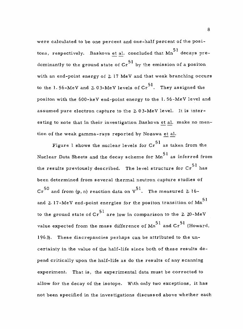
Figure 1 shows the nuclear levels for Cr51 as taken from the
Nuclear Data Sheets and the decay scheme for Mn51 as inferred from
the results previously described. The level structure for Cr51 has
been determined from several thermal neutron capture studies of
Cr50 and from (p, n) reaction data on V51. The measured 2. 16-
and 2. 17 -MeV end -point energies for the positon transition of Mn51
to the ground state of Cr51 are low in comparison to the 2. 20 -MeV
value expected from the mass difference of Mn51 and Cr51 (Howard,
1963). These discrepancies perhaps can be attributed to the un-
certainty in the value of the half -life since both of these results de-
pend critically upon the half -life as do the results of any scanning
experiment. That is, the experimental data must be corrected to
allow for the decay of the isotope. With only two exceptions, it has
not been specified in the investigations discussed above whether each
C2
7- 2
3. 13
2. 89
2. 42
2. 35
2. 03 1.92
1. 56 1. 50
1. 35
1. 17
0. 7;
9
n51 4S min
/
Cr51
/ / / / / (0.60) / /
(0. 99) / (0. 15% ß±0.05% E)
(log ft = 6. 9)
(1. 40) +
(0.36% (i , 0.04% E)
(log ft = 7. 3)
(2. 16)
(96.7%13+, 2.7% E)
(log ft = 5. 1)
Figure 1. Decay scheme of Mn51 and the low -lying levels of Cr51 5l
as summarized in the Nuclear Data Sheets.
()
5- 7-1
/
/
10 half -life value is the average of several determinations or the result
of a single measurement. Furthermore, no discussion has been
given concerning the error listed with each result. Baskova et al.
in their beta -analysis did not allow for the energy response of the
detector system, an omission of which can lead to an erroneous in-
terpretation of a beta- spectrum. The study to be described utilizes
a beta -ray scintillation spectrometer and a multichannel analyzer to
measure the end -point energy of the ground state positon transition.
This technique eliminates the need for correcting the data for the
decay of the isotope. Special consideration also is given to the beta -
spectrum to allow for the energy response of the detector system.
The log ft values calculated by Nozawa et al. for transitions to
the first two excited levels of Cr51 are large in comparison with the
value given for the ground state decay, particularly for allowed
transitions. These values of course were determined using the esti-
mated relative intensities of the 740 -keV and 1170 -keV gamma -rays.
In the investigation to be described the relative intensities of these
weak gamma -rays were experimentally measured and new log ft
values were calculated which are consisted with allowed transitions.
Prior to this investigation the spin and parity assignments for
the ground state of Mn51 and the low -lying levels of Cr51 were un-
certain. The experimental results of this study together with present
theories of nuclear models lead to unambiguous assignments of the
spin and parity of these states.
HALF -LIFE MEASUREMENT
Source Production
11
Sources of Mn51 were produced from the Cr50(d, n) reaction by
bombarding natural chromium which contains 4. 31 percent Cr50 with
7 -MeV deuterons provided by the Oregon State University cyclotron.
Chromium targets 10 mm square by 1 mm thick were exposed for 15
minutes to a 20 µA beam of deuterons. For the half -life measure-
ment and the gamma -ray analysis the Mn51 was not chemically
separated from the exposed target since no difference was observed
in either the gamma -ray spectrum or the half -life value for sepa-
rated or non -separated sources. Sources were placed on aluminum
holders which have a 1. 9 cm aperture and were mounted axially in
front of the detector.
Apparatus
Gamma rays were detected by a system consisting of a 7. 6 x
7. 6 cm NaI(T1) crystal with an "integral line" mounting on a Dumont-
6 36 3 photomultiplier, a Baird Atomic Model 31 2A Super Stable High -
Voltage power supply, a Hamner pre -amplifier and A -8 linear am-
plifier, and a Technical Measurement Corporation multichannel
analyzer operated in the multiscaler mode. The multichannel
___ _ _.... _..
12
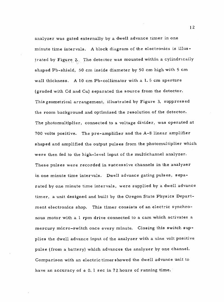
analyzer was gated externally by a dwell advance timer in one
minute time intervals. A block diagram of the electronics is illus-
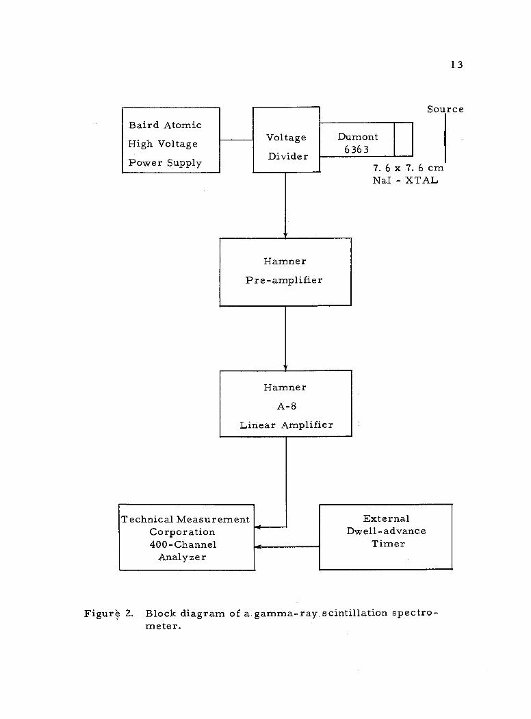
trated by Figure 2. The detector was mounted within a cylindrically
shaped Pb- shield, 50 cm inside diameter by 50 cm high with 5 cm
wall thickness. A 10 cm Pb- collimator with a 1. 5 cm aperture
(graded with Cd and Cu) separated the source from the detector.
This geometrical arrangement, illustrated by Figure 3, suppressed
the room background and optimized the resolution of the detector.
The photomultiplier, connected to a voltage divider, was operated at
700 volts positive. The pre -amplifier and the A -8 linear amplifier
shaped and amplified the output pulses from the photomultiplier which
were then fed to the high -level input of the multichannel analyzer.
These pulses were recorded in successive channels in the analyzer
in one minute time intervals. Dwell advance gating pulses, sepa-
rated by one minute time intervals, were supplied by a dwell advance
timer, a unit designed and built by the Oregon. State Physics Depart-
ment electronics shop. This timer consists of an electric synchro-
nous motor with a 1 rpm drive connected to a cam which activates a
mercury micro -switch once every minute. Closing this switch sup-
plies the dwell advance input of the analyzer with a nine volt positive
pulse (from a battery) which advances the analyzer by one channel.
Comparison with an electric timer showed the dwell advance unit to
have an accuracy of ± O. 1 sec in 72 hours of running time.
Baird Atomic
High Voltage
Power Supply
Voltage
Divider
Dumont 6363
Hamner
Pre -amplifier
Hamner
A -8
Linear Amplifier
Technical Measurement Corporation 400 - Channel
Analyzer
13
Source
7. 6 x 7. 6 cm Nat - XTAL
External Dwell- advance
Timer
Figuré 2. Block diagram of a gamma -ray scintillation spectro- meter.
Source
Pb- Shield
14
7.6x7.6 cm
NaI - XTAL
Dumont 6363
Voltage Divider
L__,,... To Pre -amp
r To Power Supply
Figure 3. Source- detector geometry for half -life analysis and gamma -ray energy measurement.
15
Experimental Results
In each half -life measurement the decay of Mn51 was followed
for 20 half- lives. Figure 4 shows a typical decay curve. After cor-
recting for background and Mn54 contamination (identified from the
gamma -ray spectrum) the natural logarithms of the counting rates
were weighted least squares fitted, as described in Appendix LE, to
determine the half -life. This calculation was performed on an IBM
1620 computer. The results of 15 measurements are listed in Table
1.
Table 1. Experimentally determined half -life values of Mn51.
Experiment Number Half -life (minutes)
1 46. 15
2 46.74
3 46.68
4 46.57
5 46. 53
6 46.63
7 46. 71
8 46.59
9 46.28
10 46. 50
11 46.50
12 46. 39
13 46.54
14 46.40
15 46. 55
Counting Rate
106
105
104
103 100 200
Figure 4. Decay curve for Mn51
300 400 Time (minutes)
500 600 700
- Corrected Data
T = 46. 5 minutes
17
An average half -life value, T, and standard deviation, 0", can be de-
termined from the following two equations,
N
(1)
(2)
where N is the number of observations, The result is T = 46. 5
± 0. 2 minutes.
- Ti) 2
= N
N
GAMMA -RAY ENERGY MEASUREMENT
Apparatus
18
Gamma -ray pulse -height spectra were recorded with the same
gamma -ray scintillation spectrometer and source -detector geometry
as described in the previous section and illustrated by Figures 2 and
3. However, the analyzer was operated in the PHA mode (pulse -
height- analyze mode) rather than the multiscaler mode, and there-
fore, the dwell advance timer was not required.
Experiment and Results
Energy calibration of the detector system was performed before
and after the recording of each Mn51 spectrum with sources of Co60,
Cs 1 37 22 54 207 Na , Mn , and Bi In order to account for any drift in
the electronics during the recording of the Mn51 spectra, the two
pulse- height spectra obtained in this procedure for each calibration
source were combined channel by channel before plotting. Figure 5
shows the result of one such energy calibration along with the tech-
nique used to determine the channel number corresponding to the
centroid of the photopeak for each calibration gamma -ray. Plotting
these channel numbers (or centroids) vs. the corresponding gamma -
ray energies provides the desired energy calibration. In this experi-
ment, however, rather than drawing a line through the calibration
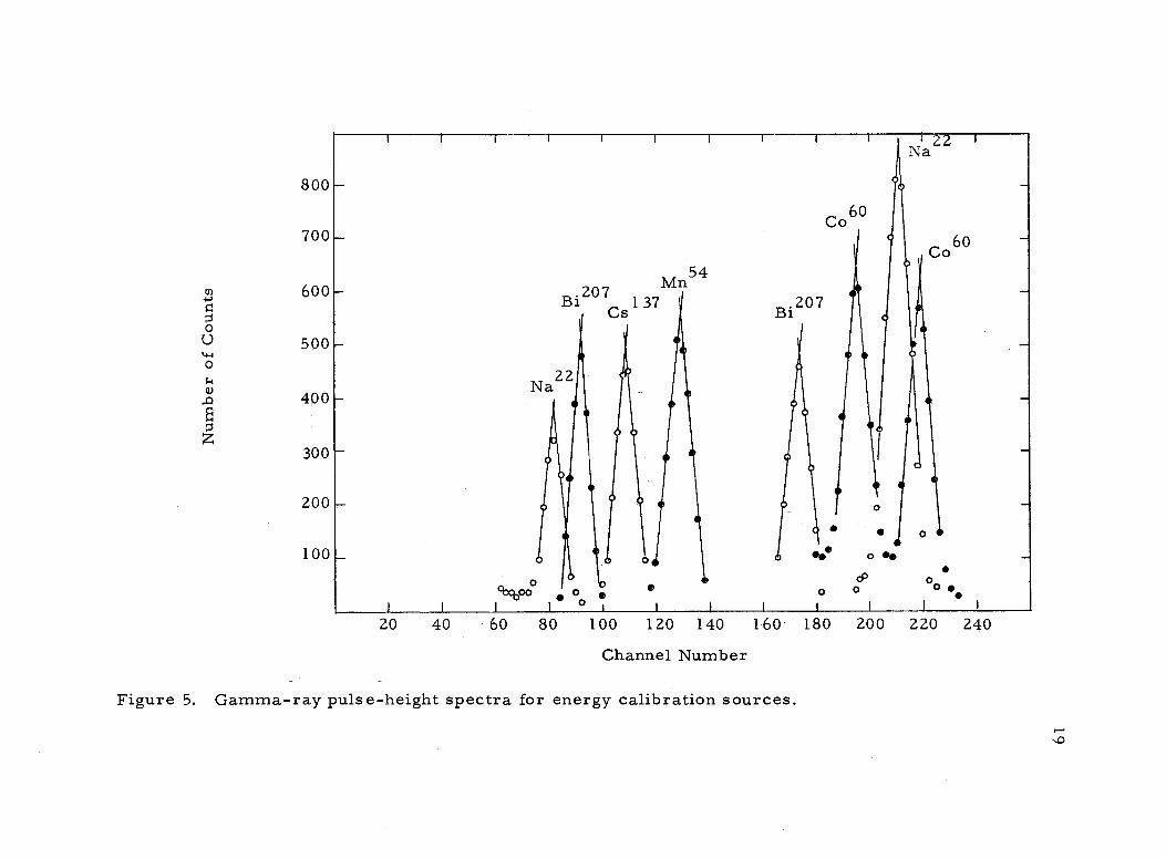
Number o
f Counts
800
700
600
500
400
300
Mn .207 137
54
4x000 o
20 40 60 80 100 120 140 160
Channel Number
Figure 5. Gamma -ray pulse- height spectra for energy calibration sources.
200 220 240
200
100
Na22
Bí207
o - cP o
0 o ° o to
I I I I ° i 1 I I i I I I
180
'-- ..o
o U
ÿ z
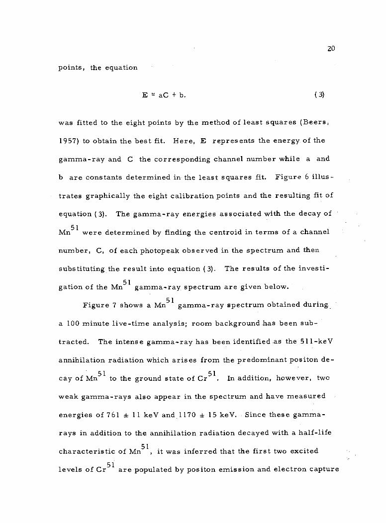
points, the equation
E=aC+b. (3)
20
was fitted to the eight points by the method of least squares (Beers,
1957) to obtain the best fit. Here, E represents the energy of the
gamma -ray and C the corresponding channel number while a and
b are constants determined in the least squares fit. Figure 6 illus-
trates graphically the eight calibration points and the resulting fit of
equation (3). The gamma -ray energies associated with the decay of
Mn51 were determined by finding the centroid in terms of a channel
number, C, of each photopeak observed in the spectrum and then
substituting the result into equation (3). The results of the investi-
gation of the Mn51 gamma -ray spectrum are given below.
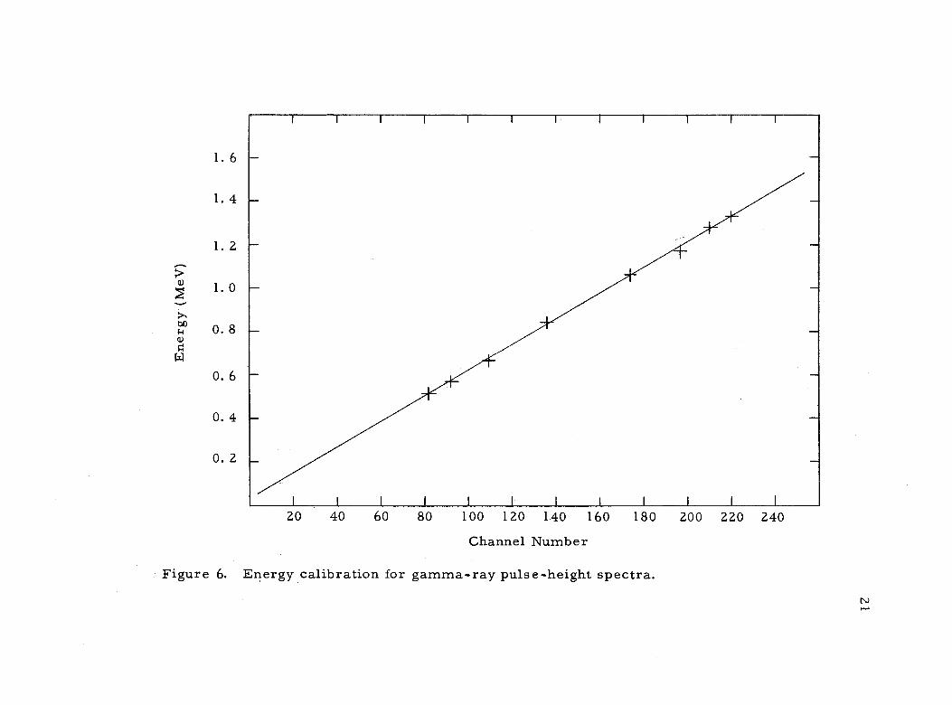
Figure 7 shows a Mn51 gamma -ray spectrum obtained during
a 100 minute live -time analysis; room background has been sub-
tracted. The intense gamma -ray has been identified as the 511 -keV
annihilation radiation which arises from the predominant positon de-
cay of Mn51 to the ground state of Cr51. In addition, however, two
weak gamma -rays also appear in the spectrum and have measured
energies of 761 * 11 keV and 1170 ± 15 keV. Since these gamma -
rays in addition to the annihilation radiation decayed with a half -life
characteristic of Mn51, it was inferred that the first two excited
levels of Cr51 are populated by positon emission and electron capture
Energy (MeV)
1. 6
1. 4
1. 2
1. 0
0. 8
0. 6
0. 4
0. 2
I I I I I I I I I I I I
20 40 60 80 100 120 140 160
Channel Number
180
Figure 6. Energy calibration for gamma -ray pulse- height spectra.
200 220 240
c)
or)
cv
W
I I I I I i i I i I i I
22
106
105
10
102
I I I I I I I I I
511-keV
o0 o
o
aoa0000axxooacbN
o 0 0
oaf)
o
o
o
o 761 -keV o
ooó 840-keV cbmo
ó°poo, 1170-keV
`00°o
I I I I I I I I I
25 50 75 100 125 150 175 200 225
Channel Number
Figure 7. Gamma -ray pulse- height spectrum for Mn51.
o
23
from the decay of Mn51. As yet, however, direct observation of the
positon -decay to these levels has not been observed. The 840 -keV
gamma -ray also present in the gamma -ray spectrum is due to Mn54
contamination.
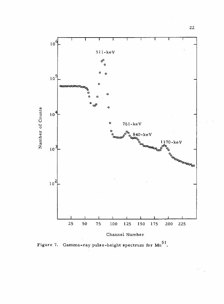
Twenty -two sources (obtained in optimizing the time and energy
of the bombardments) were analyzed in the energy measurement of
these weak gamma -rays. Table 2 lists the experimental results.
Table 2. Experimental results of gamma -ray energy measurements of Mn51.
Experiment Number Gamma -ray 1
(keV) Gamma -ray 2
(keV)
1 77 3± 10 1 177 ± 1 2
2 755 ± 10 1161±13 3 752± 9 1158±15 4 766±10 1188±13 5 768±13 1183±20 6 752 ± 11 1156 ± 17
7 769±12 1183±18 8 763 ± 14 1171 ± 21
9 766±12 1180±16 10 761 ± 14 1170 ± 21
11 767 ± 11 1181 ± 18 12 771 ± 11 1178 ± 18
13 766 * 16 1176 ± 18
14 764±13 1170 ± 20
15 769 ± 15 1181 ± 16 16 752 ± 15 1163 ± 17
17 756 ± 14 1165 ± 15
18 757± 7 1170±13 19 761 ± 8 1166 ± 14 20 760 ± 9 1161 ± 16
21 758 ± 14 1162±15 22 756± 9 1162±10
24
Associated with each energy measurement listed in Table 2 is an
error, Se, which is obtained as follows: The coefficients a and b
appearing in equation (3) have errors Sa and Sb, respectively, re-
sulting from the least squares fit. Furthermore, since the gamma -
rays were so weak, some difficulty arose in determining the cen-
troid of the photopeaks, and therefore, an error in the establishment
of C, denoted by Sc, was estimated. Including these errors, equa-
tion (3) becomes,
E fSe=(a tSa)(C fSc}+(b fSb) , (4)
from which Se evolves as,
Se = (CSa) 2 + (aSc) 2 Sb2 1
(5)
i z
Using the squared inverse of each of these errors, Se, as weighting
factors, an average energy value, r, and standard deviation, Q can
be determined from the following two equations for each of the two
weak gamma -rays,
1. Se2Wi
(32
W. i
(6)
(7)
+
e
I
('

25
where W. is the weighting factor defined previously.
The resulting values are 761 ± 11 keV and 1170 ± 15 keV.
i
26
GAMMA -RAY RELATIVE INTENSITY MEASUREMENT
Apparatus
Intensity measurements of the 761 -keV and 1170 -keV gamma -
rays relative to the positon emission were performed with the same
pulse- height gamma -ray scintillation spectrometer as described in
the previous section. However, in order to utilize the calculated
detector efficiencies given by Heath (1964) for a 7. 6 x 7. 6 cm NaI(T1)
crystal, a different source- detector geometry was required which
did not use the Pb- shield nor the collimation system previously
described. The detector was operated in a vertical position and
surrounded only by a framework to support the sources which were
mounted axially in front of the detector at a distance of 10 cm from
the face of the crystal. This particular geometry was chosen be-
cause it reproduced the system used by Heath in his gamma -ray
studies and calculation of detector efficiencies.
Experiment and Results
The relative intensity of two gamma -rays is defined simply as
the ratio of the absolute emission rate for each gamma -ray. Abso-
lute emission rates can be determined experimentally from a gamma -
ray pulse- height spectrum by using the following expression given by
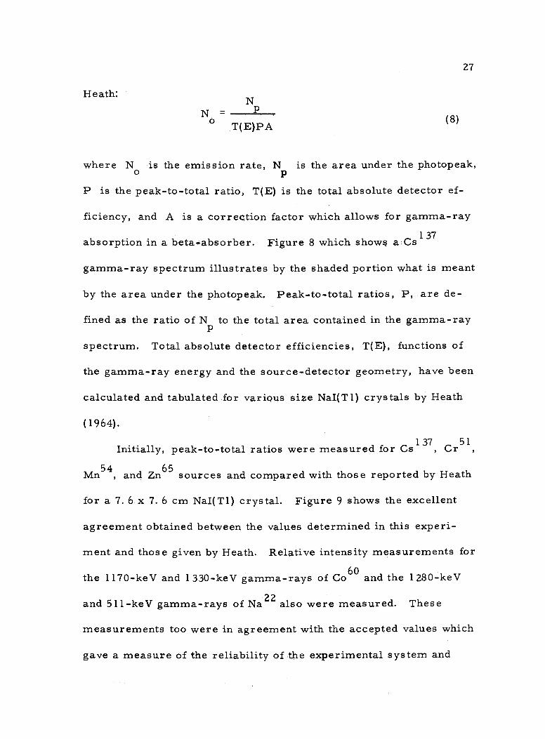
Heath: N
N = p
° T(E)PA (8)
27
where No is the emission rate, N is the area under the photopeak, p
P is the peak -to -total ratio, T(E) is the total absolute detector ef-
ficiency, and A is a correction factor which allows for gamma -ray
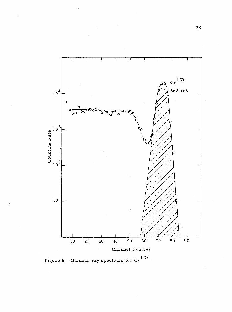
absorption in a beta- absorber. Figure 8 which shows a Cs 1 37
gamma -ray spectrum illustrates by the shaded portion what is meant
by the area under the photopeak. Peak -to -total ratios, P, are de-
fined as the ratio of N to the total area contained in the gamma -ray P
spectrum. Total absolute detector efficiencies, T(E), functions of
the gamma -ray energy and the source -detector geometry, have been
calculated and tabulated for various size NaI(T1) crystals by Heath
(1964).
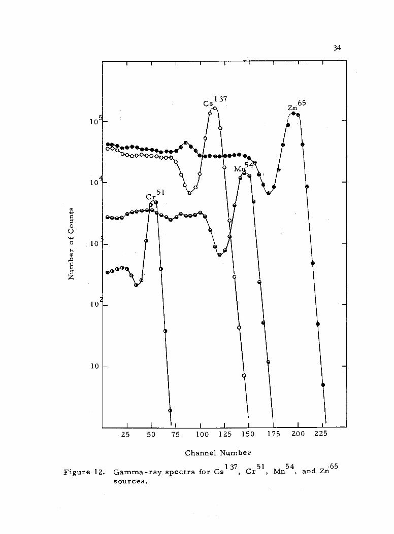
Initially, peak -to -total ratios were measured for Cs 1 37, Cr51
Mn54, and Zn65 sources and compared with those reported by Heath
for a 7. 6 x 7. 6 cm NaI(T1) crystal. Figure 9 shows the excellent
agreement obtained between the values determined in this experi-
ment and those given by Heath. Relative intensity measurements for
the 1170 -keV and 1330 -key gamma -rays of Co60 and the 1280 -keV
and 511 -keV gamma -rays of Na22 also were measured. These
measurements too were in agreement with the accepted values which
gave a measure of the reliability of the experimental system and
o
Counting Rate
104
103 4-a;
an
o U 102
10
28
10 20 30 40 50 60
Channel Number
Figure 8. Gamma -ray spectrum for Cs 1 37
70 80 90
rx
0
Peak -to -total Ratio
1. 0
0. 9
0. 8
0. 7
0. 6
0. 5
0. 4
0. 3
0. 2
0. 1
29
0. 2 0. 3 0.4 0.5
Energy (MeV)
1.0 1. 5
Figure 9. Peak -to -total ratios for a 7. 6 x 7. 6 cm NaI(T1) crystal with a 10 cm source -to- detector distance.
2
30
the techniques used in this experiment.
For the intensity measurement of the 761 -keV and 1170 -keV
gamma -rays relative to the 511 -keV gamma -ray of Mn51, the source
was placed between two Lucite absorbers with a 1.2 cm thickness.
This arrangement was designed to stop the 2. 2 MeV positons which
produced the annihilation radiation at a source -to- detector distance
of 10 cm. Since Lucite absorbers were used here, peak -to -total
ratio measurements which were described above were again made
for Csl 37, Cr51, Mn54 and Zn65 sources using a 1. 2 cm thick Lu-
cite absorber. Figure 9 shows the results which are slightly less
than the peak -to -total ratios obtained without the absorber. Corn -
paring the peak -to -total ratios obtained with and without the absorber
provides a means for determining the correction factor A listed in
equation (8).
Figure 10 illustrates a Mn51 gamma -ray spectrum obtained
with a geometry and source configuration described above during a
100 minute live -time analysis; room background has been subtracted.
Shown in this figure too are the components which contribute to the
composite Mn51 spectrum. Among these components are the 511 -keV
annihilation radiation, the 761 -keV and 1 170 -keV gamma -rays of
Mn51, an 840 -keV gamma -ray from Mn54, a bremsstrahlung distri-
bution produced by the energetic positon while passing through the
Lucite absorber, and a 1. 02 -MeV coincidence sum -spectrum due to
106
105
103
102
31
0o o 000000
o o
o 00
. 511
o
ò
o o
o
o 761
840 po0 0000
4
0 1.02 0000
ó 1. 17 0 00 00 o
o
I I I
25 50 75 100 125 150 175 200 225
Channel Number
Figure 10. Mn51 gamma -ray spectrum.
C 7
Ú 104
ó
P E
32
the intense annihilation radiation. The bremsstrahlung distribution
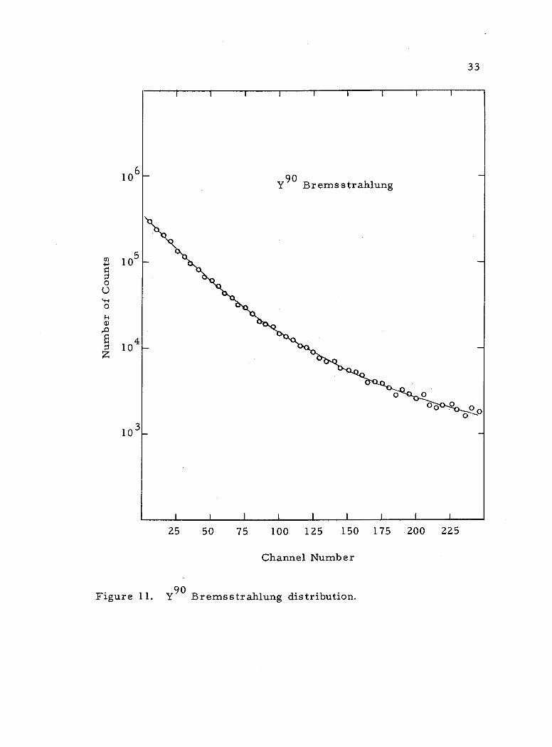
was determined experimentally with an Y90 source which emits a
beta -ray with an end -point energy of 2. 26 MeV, roughly the same as
that emitted by Mn51. Figure 11 shows the experimentally deter-
mined bremsstrahlung distribution. Gamma -ray spectra obtained
in the peak -to -total ratio measurements using a Lucite absorber are
shown in Figure 1 2 for Cs l 37, Cr51, Mn54 and Zn65 sources. The
1170 -keV component of Mn51 was approximated by the 1. 114 -MeV
spectrum of Zn65 while the 761 -keV line of Mn51 was constructed
from the 662 -keV line of Cs137 and the 840 -keV line from Mn54.
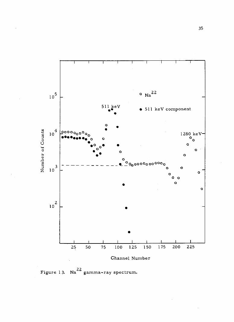
Using a Na22 gamma -ray spectrum which exhibits a 511 -keV and a
1 280 -keV gamma -ray, the 511 -keV component was obtained by ex-
tending the Compton distribution of the 1 280 -keV gamma -ray back to
zero energy and then subtracting from the composite distribution of
Na22. This procedure is illustrated in Figure 1 3 which shows a
Na22 spectrum and the resulting single 511 keV component. The
coincidence sum- spectrum, sometimes called pile -up, is produced
by two gamma -rays interacting with a crystal in a time interval
which is short compared with the resolving time of the detector.
Consequently, the detector cannot distinguish between the two gamma -
rays and the pulse -height produced is simply proportional to the sum
of the energy lost in the crystal by the two gamma -rays. In the re-
sulting spectrum one finds pulses of all sizes from the minimum
Number o
f Counts
33
25 50 75 100 125 150 175 200 225
Channel Number
Figure 11. Y90 Bremsstrahlung distribution.
Number o
f Counts
34
25 50 75 100 125 150
Channel Number
175 200 225
Figure 12. Gamma -ray . spectra for Csl 37, Cr51, Mn54, and Zn65 sources.
.
105
2 10
35
I I I I I I I I I
511 keV s
o s 000000000 00 0
0 o 0 o
o Na22
511 keV component
1280 keV- o0
o
o o °ó0000000p0000
o o o
0 0 o
o
o
o
25 50 75 100 125 150 175 200 225
Channel Number
Figure 13. Na22 gamma -ray spectrum.
Cl2 4 10
o U
o
E 3
z lo - - - -
I I I 1 I I I I I
36
detectable height to the sum of the maximum pulse -heights obtainable
from the individual gamma -rays. In the case of Mn51, the intense
51 1 -keV annihilation radiation produced the coincidence sum -
spectrum. Using the 511 -keV gamma -ray spectrum shown in Figure
13 and the techniques given by Heath (1964) the shape of the sum -
spectrum can be calculated. Let G1(a) denote the probability of de-
tecting a gamma -ray in channel a and G2(b) the probability of detect-
ing a second gamma -ray in channel b. The probabilities used here
are simply the counting rates in a particular channel number for the
given 511 -keV gamma -ray spectrum. Forming the product
G1(a)G2(b) gives the probability of detecting the sum of these two
gamma -rays in channel c for which a + b = c. The total contribution
to a particular channel c is determined by summing the product
G1(a)G2(b) over all possible pairs of a and b for which a + b = c,
that is,
S(c)
c
G1(n)G2(c - n) .
n=1
(9)
The resulting coincidence sum -spectrum obtained in this way for the
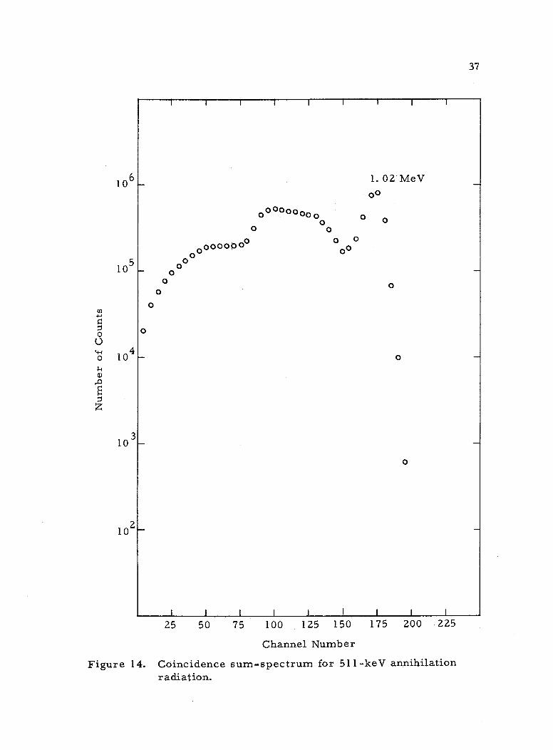
511-keV annihilation radiation is given in Figure 14.
To determine the intensity of the 761 -keV and 1170 -keV gamma-
rays of Mn51 relative to the annihilation radiation, one must unfold
the composite Mn51 spectrum, that is, determine the contribution of
=
106
105
37
103
102
o
o
o o
i I I I I I i I I
0 0 o
°0000000 o
o 0°°00000 0o
o o o o°
o
1. 02 MeV o0
o
o
o -
o
I I I I I I I I I
25 50 75 100 125 150
Channel Number
175 200 225
Figure 14. Coincidence sum -spectrum for 511 -keV annihilation radiation.
o
ó L04
-
38
each gamma -ray to the total spectrum. From the total spectrum
the bremsstrahlung distribution was subtracted after matching this
distribution with the high energy portion of the Mn51 spectrum.
Next, the 1170 -keV spectrum was subtracted after matching the
photopeak of the 1114 -keV gamma -ray of Zn65 with the 1170 -keV
photopeak appearing in the Mn51 gamma -ray spectrum minus the
bremsstrahlung distribution. In successive order, the contribution
of the coincidence sum -spectrum, the 840 -keV line, the 761 -keV
line, and the 511 -keV gamma -ray were subtracted. Figure 10 shows
the result of the unfolding process. For each of the 511 -keV, 761 -
keV, and 1170 -keV gamma -rays shown in Figure 10, the area under
the photopeak, N , was calculated. Using these values of N , the P P
peak -to -total ratios from Figure 9 for gamma -ray energies of 511
keV, 761 keV, and 1170 keV, and the tabulated values of the absolute
detector efficiencies, T(E), given by Heath (1964), the absolute
emission rate No for each of the gamma -rays listed above was de-
termined from equation (8). Once these values No were calculated,
the relative intensities of the 761 -keV and 1170 -keV gamma -rays to
the 511 -keV annihilation radiation were computed by taking the ratios
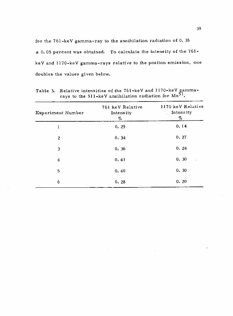
of No. Table 3 lists the experimental results of six measurements.
From these measurements an average value and error for the in-
tensity of the 1170 -keV gamma -ray relative to the 511 -keV annihila-
tion radiation of 0. 24 0. 06 percent was determined while the value t
39
for the 761 -keV gamma -ray to the annihilation radiation of 0. 35
± 0. 05 percent was obtained. To calculate the intensity of the 761 -
keV and 1170 -keV gamma -rays relative to the positon emission, one
doubles the values given below.
Table 3. Relative intensities of the 761 -keV and 1170 -keV gamma - rays to the 511 -keV annihilation radiation for Mn 1.
Experiment Number 761 keV Relative 1170 keV Relative
Intensity Intensity
1 0. 29 0. 14
2 0. 34 0. 27
3 0. 36 0. 24
4 0. 41 0. 30
5 0. 40 0. 30
6 0. 28 0. 20
END -POINT ENERGY MEASUREMENT
Apparatus
40
The investigation of the end -point energy of the positon which
decays to the ground state of Cr51 was performed with a beta -ray
scintillation spectrometer and a beta -gamma coincidence scintilla-
tion spectrometer. Figure 15 gives a block diagram of the elec-
tronics for the beta -gamma coincidence spectrometer which is easily
converted to a beta -ray spectrometer by removing the gating signal
supplied to the multichannel analyzer and the coincidence require-
ment on the analyzer. Beta -rays were detected with a 3. 8 x 2. 5 cm
Pilot -B plastic scintillator optically coupled to an RCA 6655A photo -
multiplier while gamma -rays were detected with a 3. 8 x 2. 5 cm
NaI(T1) crystal optically coupled to an RCA 6655A photomultiplier.
In order to avoid absorption in a crystal covering these detectors
which had an angular separation of 90° were mounted inside a light -
tight enclosure. Sources were prepared as described in Appendix I
and mounted 2 cm from the Pilot -B detector and 10 cm from the
NaI(T1) detector. The coincidence spectrometer was used only in
the study of line shapes for monoenergetic electrons supplied by con-
version electrons from sources of Cs 1 37 and Bi207 and operated in
the following manner: Voltage pulses from the photomultipliers,
resulting from the interaction of beta -rays and gamma -rays with the
a
High Voltage Power Supply
2
Voltage Divider
2
2
RCA 6655A
Hamner Pre -amplifier
2
Hamner A -8
Linear Amplifier
2
NaI
Source 1
{
High Voltage Power Supply
1
RCA 6655A
Pilot -B
= 300 nsec
Voltage Divider
1
Hamner Pre -amplifier
1
Coincidence
Hamner A -8
Linear Amplifier
1
Slow
Coincidence
Scaler Scaler
41
2 µsec Delay
Technical Measurement Corporation 400 - channel
Analyzer
Figure 15. Block diagram of a beta -gamma coincidence spectro- meter.
1
Fast
Hamner
Differential
Discriminator
Y
J (o°
42
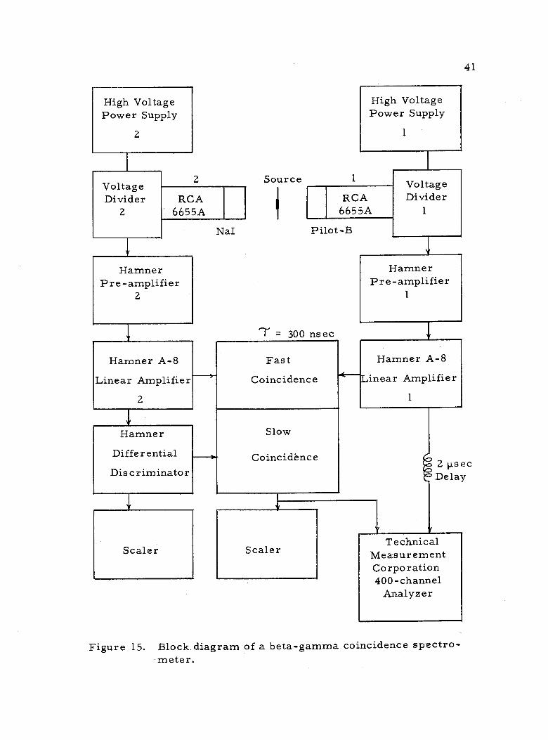
Pilot -B and NaI(T1) scintillators, respectively, were amplifed by
two Hamner pre -amplifiers and A -8 linear amplifiers. From these
signals, gating pulses were formed in each of the linear amplifiers
and fed into the fast coincidence unit where an output pulse resulted
if the two gating signals, one from each amplifier, arrived at the
fast coincidence unit within a resolving time of 300 nsec. In addition
to demanding fast coincidence, the system also required the pulses
from detector 2 to satisfy a certain energy requirement which was
provided by a differential energy discriminator whose baseline and
window width were adjusted to bracket just the photopeak of the
gamma -ray for which the beta -rays are in coincidence. The output
of the differential discriminator was split to feed the slow coinci-
dence circuit. Because the signal was divided in this manner, every
signal from the differential discriminator provided the coincidence
requirements necessary to trigger the slow coincidence unit. If the
coincidence requirements were satisfied in both the fast and slow
units by the occurrence of two events, one in detector 1 and the other
in detector 2, then a gating pulse was supplied to the multichannel
analyzer which turned the analyzer on for a duration of 4 µsec, a
period during which a pulse coming from linear amplifier 1 could be
recorded. As shown in Figure 15, the pulses coming from amplifier
1 were delayed by 2 µsec to allow for the inherent time required to
generate the gating pulse for the multichannel analyzer.
43
Experiment and Results
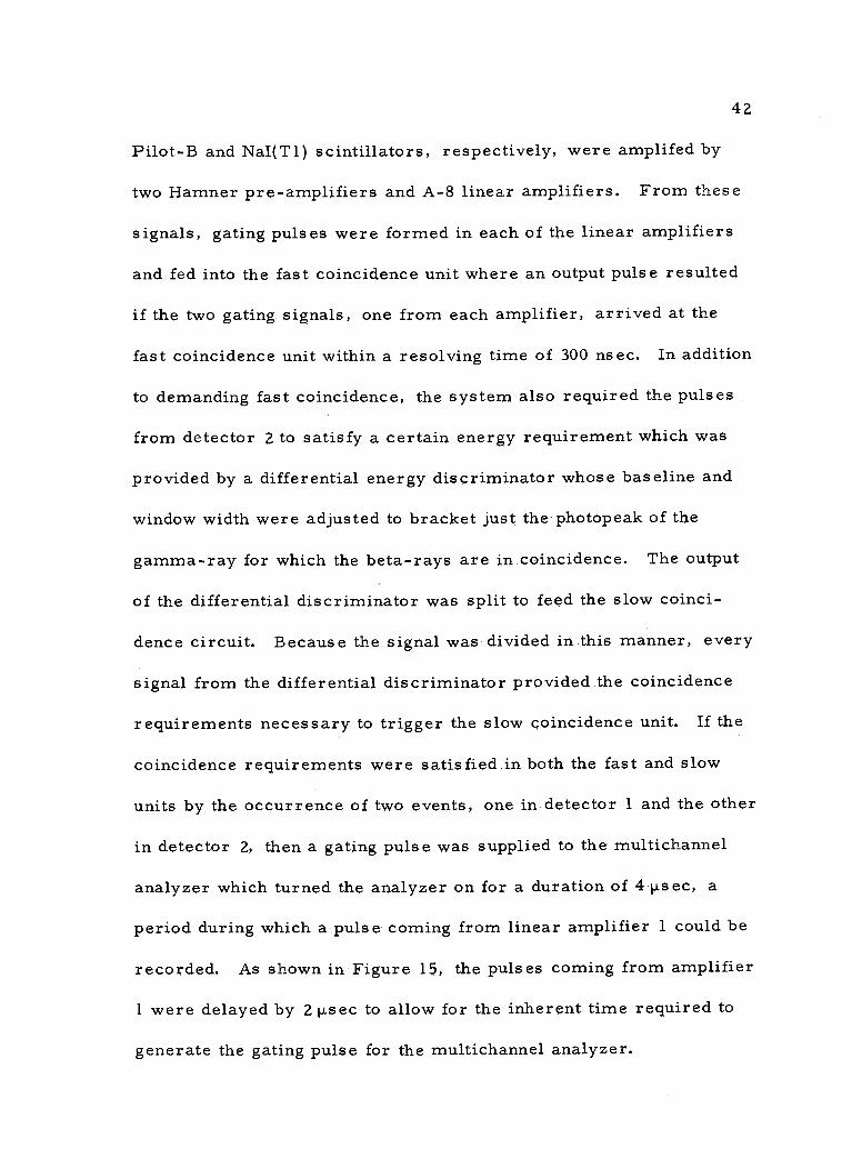
The beta -ray scintillation spectrometer was energy calibrated
with conversion electrons from sources of Cs 1 37 and Bi207; the
Pilot -B scintillator had an energy resolution of 15 percent for the
624 -keV K- conversion line from Cs137. Figure 16 shows typical
beta -ray spectra used for energy calibration. In addition to Cs137
and Bi207, calibration was also provided by sources of Y90 and P32
with end -point energies of 2. 26 MeV and 1. 704 MeV, respectively.
In the measurement of end -point energies of beta -rays and
positons a difficulty arises which cannot be neglected; the recorded
energy spectrum is not the true spectrum emitted by the source.
This difference is illustrated most easily by Figure 17 which shows
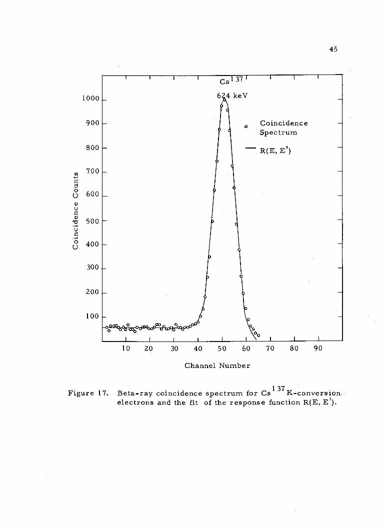
the energy response of a Pilot -B scintillator to a source of mono-
energetic electrons from Cs 1 37. Centered around the energy
624 keV, the energy of the conversion electrons, is the normal sta-
tistical broadening which is approximately gaussian in shape (Palmer
and Laslett, 1951). Along with this factor, however, is a low in-
tensity backscatter contribution extending to zero energy caused by
the electrons losing only part of their energy in the detector, the
remainder being scattered out. Because of this energy response, a
continuous beta -spectrum recorded in an experiment will exhibit a
greater number of counts in the low energy part of the spectrum than
Num
ber
of C
ount
s
(Aay
AI)
A
$aau
a
900
800
700
600
500
400
300
200
100
1. 8
1. 6
1. 4
1. 2
1. 0
0. 8
0. 6
0. 4
0. 2
20 40 60 80 100 Channel Number
Figure 16. Beta -ray spectra for Cs 1 37 and Bi207 and energy calibration.
Coincidence Counts
45
1000 -
900 -
800 -
700 -
600 _
500 -
400 -
300 -
200 -
100 -
Cs 37
624 keV
o
ó o
I I I I I I o I I I
Coincidence Spectrum
R(E, E')
10 20 30 40 50 60 70 80 90
Channel Number
Figure 17. Beta -ray coincidence spectrum for Cs 1 37 K- conversion.
electrons and the fit of the response function R(E, Et).
o
46
in the true energy spectrum while the high energy portion will be
lacking counts. This effect of course can lead to an erroneous in-
terpretation of the Kurie plot which will be discussed later. The
energy response to the 624 -keV conversion electron shown on Figure
17 actually represents the probability, R(E, E'), of recording the
energy of an electron of energy E' in an energy interval E to E +AE.
Thus, it is imperative in the investigation of continuous beta -spectra
to determine the energy response function R(E, E') for various ener-
gies E'. The response function, R(E, E'), the experimental spec-
trum, M(E) and the true energy spectrum, N(E'), are related by the
following expression:
e max M(E) = C R(E, E')N(E')dE'.
0
(10)
Using the numerical approximation technique suggested by Freedman
et al. (1956) and a high speed computer, the true energy spectrum
can be determined from equation (10). This process is described
completely in Appendix IV.
To determine the response function R(E, E') , line shapes from
monoenergetic electrons were examined using beta -gamma coinci-
dence techniques. The 624 -keV K- conversion electron from Cs 1 37
was isolated from the continuous beta -spectrum and the L- conversion
electron by demanding coincidence between the conversion electron
47
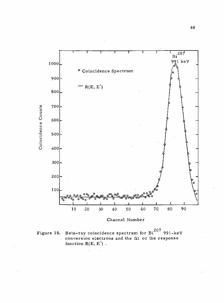
and the Bat 37 x -ray. In a similar study conversion electrons
from Bi207 two additional lines. The 991 -keV line of Bi207
(average energy of the K and L conversion electrons with K/L = 3. 5)
was observed in coincidence with the 570 -keV gamma -ray while the
499 -keV line (average energy of the K and L conversion electrons
with K/L = 3. 4) was separated by demanding coincidence with the
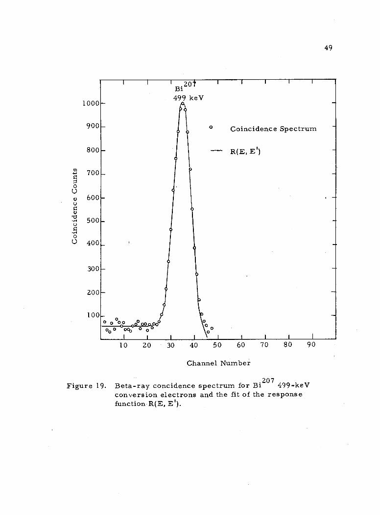
1064 -keV gamma -ray. Figures 17, 18 and 19 show the coincidence
spectra for these three energies, respectively. Note that the ratio
of the height of the backscatter tail to the height of the photopeak is
about the same for all three spectra.
Using these three experimentally determined line shapes and
the arguments of Palmer and Laslett (1951) that the photopeak is ap-
proximately gaussian shaped and the half- width, a, at 1/e of the
height of the photopeak varies as the square root of the electron
energy E', the following response function, R(E, E'), was con-
structed:
k.+(1 -rri)e-(E-E1)2¡a2 R(E'E) kE'+afTf - ? ma V
where E' = maximum kinetic energy of the conversion electron,
k = constant for 0 < E < E',
k 0 for all other E,
m = constant for E E',
provided
=
$
Coi
ncid
ence
Cou
nts
1000
900
800
700
600
500
400
300
200
100
o Coincidence Spectrum
0 0 000 0 0 OO 0n03 0° 00 i W O
O u 00 0000 0 O '(P0 O o
I I I I
10 20 30 40
Bi20/ 991 keV
os)
48
0po o
I I
50 60
Channel Number
o
1
7Q 80 1
90
Figure 18. Beta -ray coincidence spectrum for Bi207 991 -keV conversion electrons and the fit or the response function R(E, E') .
R(E, E')
I
C 7 0
o
Coi
ncid
ence
Cou
nts
1000
900
800
700
600
500
400
300
200
100 o 0 0 000
000 \ o 000 0 0 00 oo
I I I I I I I I I
I Bi20f 499 keV
o
49
Coincidence Spectrum
- R(E, Et)
10 20 30 40 50 60 70 80 90
Channel Number
Figure 19. Beta -ray concidence spectrum for Bi207 499 -keV conversion electrons and the fit of the response function R(E, E').
50
m = O for E >E',
a a +biE' ,
a = constant,
b = constant.
This response function which has been normalized to unity was con-
structed in the following manner: For electron energies in the en-
ergy spectrum greater than E', a pure gaussian function was fit,
while on the low- energy side of E', the response function consists of
a constant intensity backscatter component of height k, the frac-
tional height of the photopeak, extending from zero energy to the con-
version electron energy E', and a gaussian distribution. The gaus-
sian distribution on the low energy side is the same as that fit to
the high energy side of E', but is multiplied by a constant (1 m)
such that the sum of the gaussian component and the backscatter
component will match the fit of the high energy side at E'. A non-
zero value of 0. 055 was determined from Figures 17, 18 and 19 for
the parameters k and m which differ only in their range of definition.
Included in each of the Figures 17, 18 and 19 is the fit of the re-
sponse function R(E, E') to the given spectrum.
Even though the response function formulated above fits the
three line shapes in the energy region below 1000 keV quite well,
its use in equation (10) and its application to higher energy regions
was carefully checked. Its application to higher energy regions was
-
51
justified using sources of P32 and Y90 which have end -point energies
of 1. 704 MeV and 2. 26 MeV, respectively. Before discussing this
check, however, we must first consider the following.
From the theory of beta -decay the distribution of electron en-
ergies which arise from a continuous beta -emitter can be repre-
sented by (Howard, 1963):
N(W)dW = Kiw(W)F(Z, W)pW(Wo - W)2dW, (1 2)
where N(W)dW = the number of electrons with energy in the inter- val W to W + dW,
W = total energy of electron emitted including its mass energy,
w(W) = shape factor which is equal to unity for allowed transitions and equal to (W2 - 1) + (W
0 W) 2 for
first forbidden transitions,
p = electron momentum,
W 0
maximum electron energy,
F(Z, W) = "Fermi Function" which takes account of the coulomb field of the daughter nucleus of atomic number Z.
Transforming equation (1 2) gives the following;
N(W)dW = K(W - W)2dW . w(W)F( Z, W)p W o (1 3)
From equation (1 3) it is clear that a plot of N(W) vs. W w(W) F( Z, W)p W
2 or W - m 0
c yields a linear curve in W. By extending this curve to
-
=
i z
52
where N( W)
w( W) F( Z, W)pW becomes zero, that is, at W = Wo,
provides a means for determining the end -point energy, W -m c 2, o o
of the electron. This is the plot which is defined as the Kurie plot in
the analysis of continuous beta -spectra.
The Fermi functions, F(Z, W), appearing above, functions of
the atomic number, Z, of the daughter nucleus and the total energy
W of the electron have been tabulated for numerous nuclei and elec-
tron energies (Siegbahn, 1964). In some cases rather than tabulating
the Fermi function, F(Z, W), however, a "reduced Fermi function ",
f(Z, W), is listed which is related to the Fermi function F(Z, W) by
the following expression,
f( Z, W) = p 2F( Z, W). (14)
Thus, a plot of N(W)P vs. W gives the desired Kurie [w(W)W1 plot. The end -point energy is determined by substituting the true
energy spectrum into the expression above for N(W) and, using ap-
propriate tabulated reduced Fermi functions, making a Kurie plot.
As mentioned previously the experimental approach and pro-
cedure used in this investigation was justified with sources of P32
and Y90 which have end -point energies of 1. 704 MeV and 2. 26 MeV,
respectively. Calibrating the system with the conversion electrons
from Bi207 and Cs 1 37, the experimental beta -spectra for sources of
P32 and Y90 were recorded. Using the response function (11),
i
i
]
2
53
equation (10), and the procedure presented in Appendix IV, the true
energy spectra for both sources were determined. Kurie plots,
formed from these true energy spectra, were linear in energy (al-
lowing for the forbidden shape of Y90) and gave end -point energies of
1. 70 MeV and 2. 26 MeV for P32 and Y90, respectively. These re-
sulting end -point energies and linear Kurie plots rendered support
for the response function and the correction process used to deter-
mine the true energy spectrum, Figures 20 and 21 show the Kurie
plots for P32 and Y90 sources before and after subjecting the experi-
mental spectra to the correction process. Clearly, without correct-
ing for the energy response of the detector, the Kurie plots are not
linear and lead to complications in determining the end -point energy
and the nature of the decay, whether it is complex or not.
In a similar manner the end -point energy of the positon decay-
ing from Mn51 to the ground state of Cr51 was measured. Since
Mn51 is a positon emitter the beta -spectrum also contained a con-
tribution due to annihilation radiation. The contribution to the beta -
spectrum from the gamma -rays was determined by inserting a Lu-
cite absorber between the source and the detector to absorb the beta -
rays. Subtracting the gamma- spectrum from the composite gamma -
and beta -ray spectrum recorded without the absorber produced the
pure Mn51 beta -spectrum.
In analysing these continuous beta -spectra, the data points
.Np wfW
90
80
70
60
50
40
30
20
10
Figure 20.
40 60 80 100 120
Channel Number
140 160 180
Kurie plots for P32 with and without correcting the experimental spectrum for the detector response. Ui
4
1,32
O with correction
without correction
1. 70 Me V
90
80
70
60
Np 50 wfW
40
30
20
10
20 40 60 80 100 120 Channel Number
140 160 180 200
Figure 21. Kurie plots for Y90 with and without correcting the experimental spectrum for the detector response. u-
v1
56
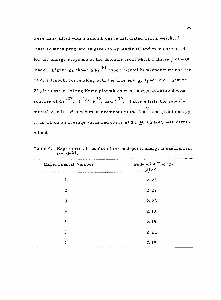
were first fitted with a smooth curve calculated with a weighted
least squares program as given in Appendix III and then corrected
for the energy response of the detector from which a Kurie plot was
made. Figure 22 shows a Mn51 experimental beta - spectrum and the
fit of a smooth curve along with the true energy spectrum. Figure
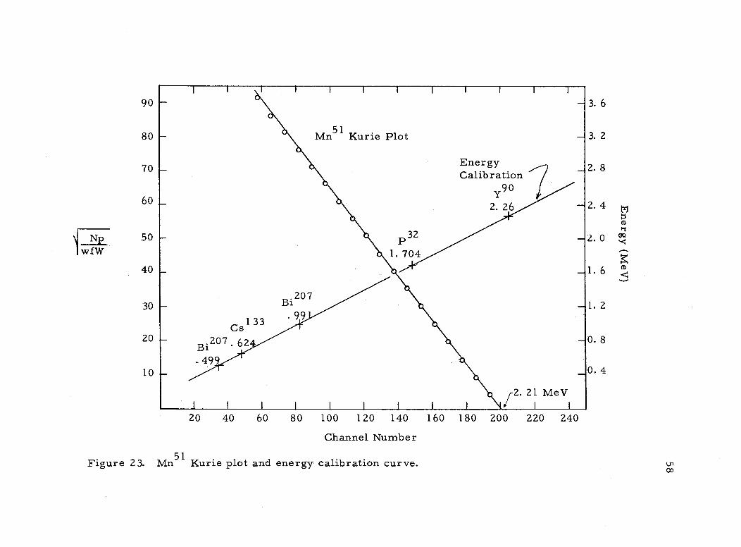
23 gives the resulting Kurie plot which was energy calibrated with
sources of Cs Bi207 P32, and Y90. Table 4 lists the experi-
mental results of seven measurements of the Mn51 end -point energy
from which an average value and error of 2.21 +0. 02 MeV was deter-
mined.
Table 4. Experimental results of the end -point energy measurement for Mn51.
Experimental Number End -point Energy (MeV)
1
2
3
4
5
7
2. 22
2. 22
2. 22
2. 18
2. 19
2. 22
2. 19
6
Number o
f Counts
9000
8000
7000
6000
5000
4000
3000
2000
1000
51 Mn S 00
O O O O O - o o
O
o o
o Experimental Spectrum
True Energy Spectrum
- o
o o
_ o o o
o
_ o
o
o o
o 0
o - o
o o - o -
o o
o o o o
I I
Figure 22.
20 40 60 80 100 120
Channel Number
140 160 180
Mn51 experimental beta -spectrum and the calculated true energy spectrum.
200
o _
i o
(AaN
I) a
aaua
90
80
70
60
Np 50 wfW
40
30
20
10
20 40 60 80 100 120 140
Channel Number
160 180 200 220 240
3. 6
3. 2
2. 8
2. 4
2. 0
1. 6
1. 2
0. 8
0. 4
Figure 23. Mn51 Kurie plot and energy calibration curve. u-i oo
59
MEAN -LIFE TIMES OF THE 761 -keV AND 1170 -keV LEVELS OF Cr -51
Apparatus
The mean -lives of the 761 -keV and 1170 -keV levels of Cr51
were investigated with a delayed coincidence spectrometer. A de-
tailed description of this spectrometer, the procedure for time cali-
bration, and the methods used in interpreting the experimental re-
sults are given by Sommerfeldt (1964).
Experiment and Results
Sources of Mn51 were first placed between two aluminum ab-
sorbers, each having a 2. 5 cm thickness which was sufficient to
stop the most energetic positons. The sources were then mounted
between two gamma -ray detectors which had an angular separation
of 180'.
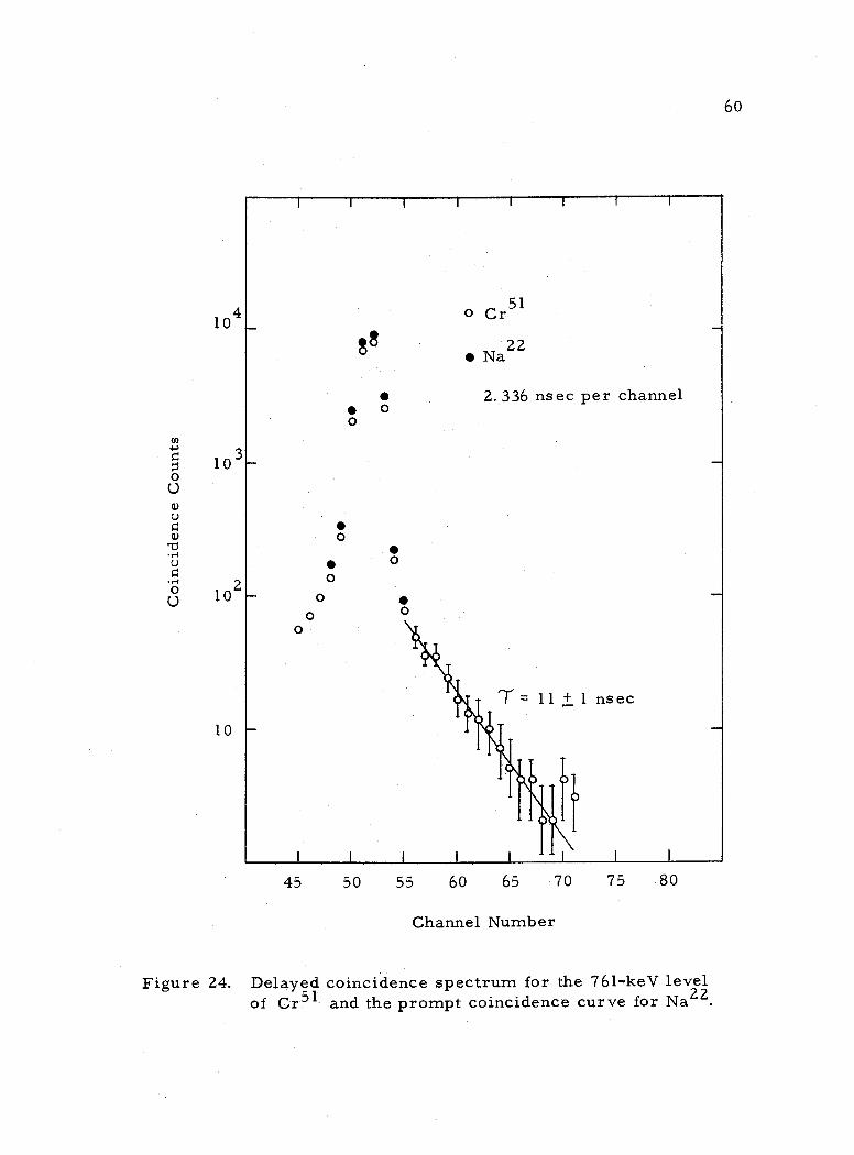
For the mean -life measurement of the 761 -keV level, the
spectrometer was gated on the coincidence between the 511 -keV an-
nihilation and the 761 -keV gamma -rays. The delayed coincidence
spectrum obtained for Cr51 is shown in Figure 24 along with a
prompt coincidence curve obtained for Na22 using the same spectro-
meter settings. Measuring the slope of the delayed coincidence
spectrum in the region beyond the prompt coincidence curve using
Coincidence Counts
60
104
103
102
10
45 50 55 60 65 70 75 80
Channel Number
Figure 24. Delayed coincidence spectrum for the 761 -keV level of Cr51 and the prompt coincidence curve for Na22.
61
the method of least squares provided a means for determining the
mean -life of the 761 -keV level. From Figure 24 a mean -life of
11 f 1 nsec was measured for this level.
In a similar manner the mean -life of the 1170 -keV level was
investigated. For this measurement the spectrometer was gated on
the coincidence between the 511 -keV and 1170 -keV gamma -rays; this
procedure yielded a delayed coincidence spectrum which did not dif-
fer from the prompt coincidence curve obtained for Na22 using the
same spectrometer settings. Both coincidence spectra are shown
in Figure 25 from which the mean -life of the 1170 -keV level of Cr51
has been estimated to have an upper -limit of one nanosecond.
Coi
ncid
ence
Cou
nts
104
103
102
10
i t
o
o o
Ir
Cr51
Na22
1. 168 nsec per channel
o -
0 0 0 0 0
00 0 0 0 0 0
0 0 0
o
I I I I I I I I
95 100 105 110 115 120 125 130
Channel Number
62
Figure 25. Delayed coincidence spectrum for the 1170 -keV level of Cr51 and the prompt coincidence curve for Na22.
I i i i
ó 0
o ó
°
63
CONCLUSIONS
The experimental results discussed in the previous sections
are combined with theory in this section in order to make spin and
parity assignments for the ground state of Mn51 and to the low -lying
levels of Cr51 inasmuch as spin and parity are the nuclear para-
meters which one compares with the predictions of the shell model.
To make these assignments, however, additional properties are
required which can be calculated from theory using the experimental
results as a basis. Among these properties are the log ft values,
transition probability ratios, branching intensities, mean -life times
of excited nuclear states, and the multipolarity of the gamma -radi-
ation. Log ft values, the common logarithm of the comparative
half- periods, ft, are fundamental in determining the character of
beta -decay, that is, the degree of forbiddeness of the transition.
Beta -transitions are classified as allowed for log ft values in the
region 3 to 6 and first -forbidden for values in the range 6 to 10.
According to Gamow- Teller selection rules, allowed transitions
have no parity change and spin changes limited to 0 or ± 1 units,
while first -forbidden transitions have a parity change and spin
changes restricted to 0, ± 1, or ± 2 units. The comparative half -
period, ft, appearing in log ft, is the product of the integral Fermi
function, f, and the partial half -period, t, of the transition.
64
Transition probability ratios which are necessary in determining the
branching intensities simply compare the probabilities for electron
capture and positon emission to a definite energy state. The branch-
ing intensity is defined as the fractional number of transitions going
to a particular energy level for a given number of decays. This
includes transitions by electron capture and positon emission if the
latter is energetically possible. The mean -life time of an excited
nuclear state is defined as the average time interval that a nucleus
remains in a specific energy level before decaying by gamma -
emission to a lower energy state. Gamma -radiation emitted in the
decay cay be either electric or magnetic multipole radiation with
different orders of multipolarity. The multipolarity and the mean -
life time are related; the longer the life -time, the higher the order
of the multipolarity. Associated 'with multipole radiation are defi-
nite rules governing changes of parity and spin. For this reason
one attempts to determine the multipolarity of the radiation emitted
and to distinguish between electric and magnetic radiation in order
that spin and parity assignments can be made. In the discussion
which follows, numerical values are determined and tabulated for
the parameters which characterize the strong transition to the
ground state of Cr51 and the weak population of the 761 -keV and
1170 -keV levels of Cr51 in the decay of Mn51. In some cases, how-
ever, numerical values have been calculated for the parameters
65
describing possible transitions to energy states higher than 1170 -keV
in Cr51. This has been done mainly to justify why evidence of these
transitions are not observed in this experiment. The decay scheme
shown in Figure 26 summarizes the results of this section along with
the experimentally determined properties previously discussed.
Basic to the calculation of log ft values and branching intensi-
ties for transitions to each level shown in Figure 26 are the ratios
of the transition probabilities for electron capture to positon emis-
sion, or equivalently, the ratios of the integral Fermi functions for
electron capture to positon emission. Tabulated values for these
ratios calculated from theory exist for a certain number of positon
energies and daughter nuclei. For intermediate energies and atomic
numbers one is required to use linear interpolation. The procedure
followed here utilizes the tabulated ratios and linear interpolation
method given by Wapstra et al. (1959). Table 5 lists the results.
In addition to the ratio of the transition probabilities for electron
capture to positon emission, denoted by f /f the quantities fE /f E
and f f, the ratios of the electron capture and positon emission
transition probabilities to the total transition probability, respective-
ly, also are included. The integral Fermi function, f, is just the
sum off and f For transitions to energy states higher than E
2. 03 MeV in Cr51, positon emission is energetically forbidden and
the decay is by pure electron capture. This fact is indicated in
3.13
2.89
2.42 2. 35
2.0 3
1.92
1.56 1.50
1.35
C5- 7-\ 1.170 2 ' 2 )
66
/ /
/ / / /
/ (< 1 ns ec) /
7- 2
Cr
(1.04 MeV) (0. 337% ß +, 0.124% e) (log ft =5.14)
(1.45 MeV) (0.594% .13+,0.079% E)
(log ft = 5.49)
(2.21 MeV) (95.2% ß +, 3.66% e) (log ft = 5. 07)
Figure 26. Decay scheme for Mn51 (present investigation).
n51 46.5 min
j /
(ll naPr) I
E2
(2 / n 961
5-
2 /
// // //
/ / /
67
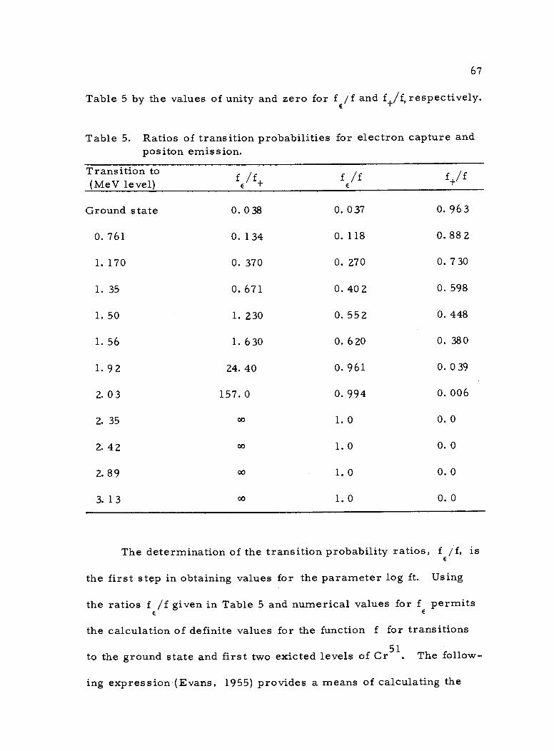
Table 5 by the values of unity and zero for f E /f and f /f
+ ' respectively.
Table 5. Ratios of transition probabilities for electron capture and positon emission.
Transition to (MeV level) fE/f+ fE/f f+/f
Ground state 0.038 0. 037 0. 963
0. 761 0. 1 34 0. 118 0. 88 2
1. 170 0. 370 0. 270 0. 7 30
1. 35 0. 67 1 0. 40 2 0. 598
1. 50 1. 230 0. 552 0. 448
1. 56 1. 630 0.620 0.380
1.92 24. 40 0. 961 0.039
2.03 157. 0 0. 994 0. 006
2. 35 00 1.0 0.0
2.42 00 1.0 0.0
2.89 00 1.0 0.0
3. 1 3 00 1.0 0.0
The determination of the transition probability ratios, f /f, is E
the first step in obtaining values for the parameter log ft. Using
the ratios f /f given in Table 5 and numerical values for f permits E E
the calculation of definite values for the function f for transitions
to the ground state and first two exicted levels of Cr51. The follow-
ing expression (Evans, 1955) provides a means of calculating the
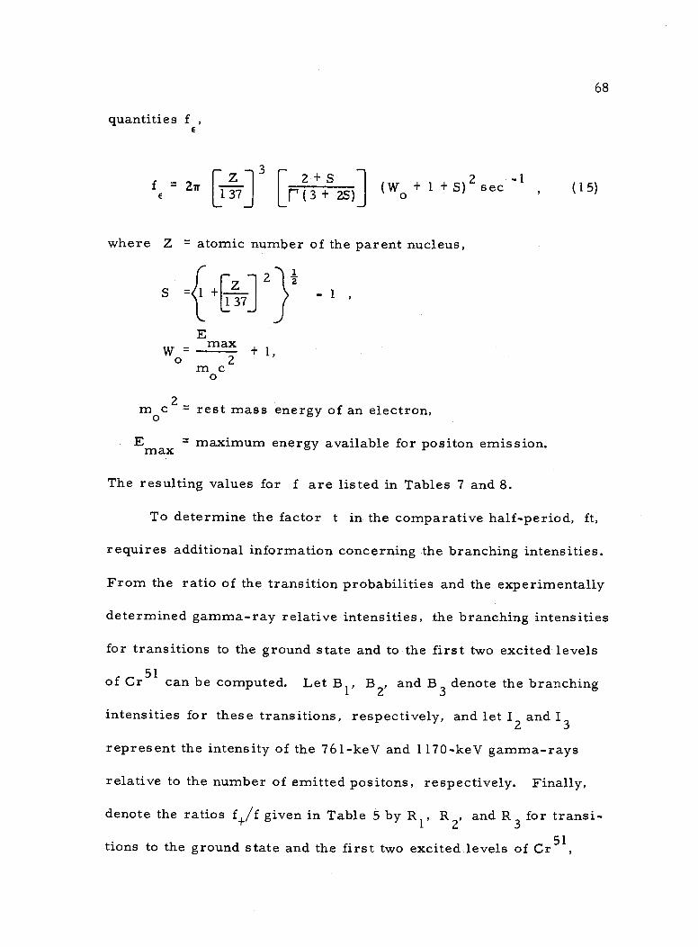
quantities f , E
3 +
fE = 27r 13 j,(3 S25) (Wo + 1+ S)2 sec -1
where Z = atomic number of the parent nucleus,
2 Z S = 1+137
E max
C o
+ 1,
- 1 ,
moc 0
2 = rest mass energy of an electron,
maximum energy available for positon emission. max
68
(15)
The resulting values for f are listed in Tables 7 and 8.
To determine the factor t in the comparative half- period, ft,
requires additional information concerning the branching intensities.
From the ratio of the transition probabilities and the experimentally
determined gamma -ray relative intensities, the branching intensities
for transitions to the ground state and to the first two excited levels
of Cr51 can be computed. Let B1, B2, and B3 denote the branching
intensities for these transitions, respectively, and let 12 and I3
represent the intensity of the 761 -keV and 1170 -keV gamma -rays
relative to the number of emitted positons, respectively. Finally,
denote the ratios f +/f given in Table 5 by RI, R2, and R3 for transi-
tions to the ground state and the first two excited levels of Cr51,
W - 0
m
=
69
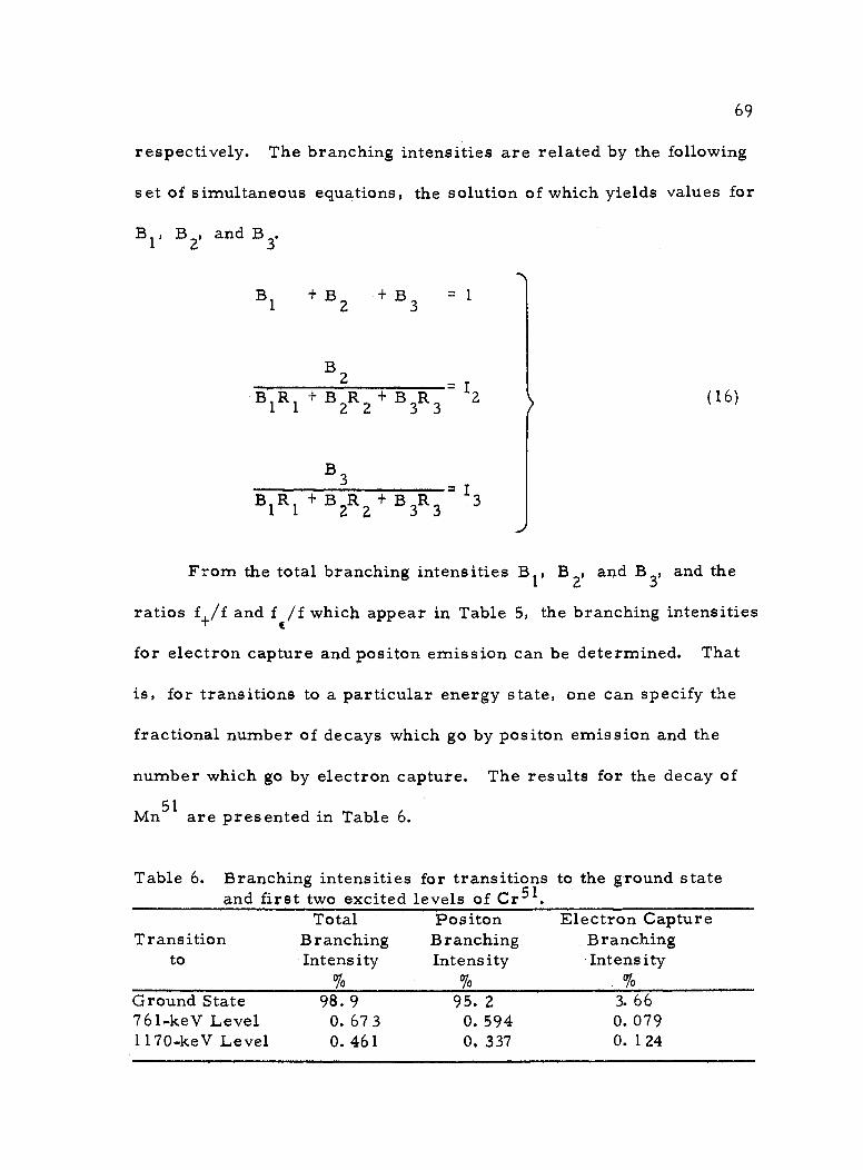
respectively. The branching intensities are related by the following
set of simultaneous equations, the solution of which yields values for
B1, B2, and B3.
B1 +B2 +B3 - 1
B2
+ B2R2+ B3R3 I2
B3
+ B2R2 + B3R3 - I3
(16)
From the total branching intensities B1, B2, and B3, and the
ratios f +/f and f /f which appear in Table 5, the branching intensities E
for electron capture and positon emission can be determined. That
is, for transitions to a particular energy state, one can specify the
fractional number of decays which go by positon emission and the
number which go by electron capture. The results for the decay of
Mn51 are presented in Table 6.
Table 6. Branching intensities for transitions to the ground state and first two excited levels of Cr51.
Total Positon Electron Capture Branching Branching Intensity Intensity
Transition to
Branching Intensity
Ground State 98. 9 95. 2 3. 66 761 -keV Level 0. 67 3 0. 594 0. 079 1170 -keV Level 0. 461 0. 337 0. 1 24
B1R1
% % %
B1R1
70
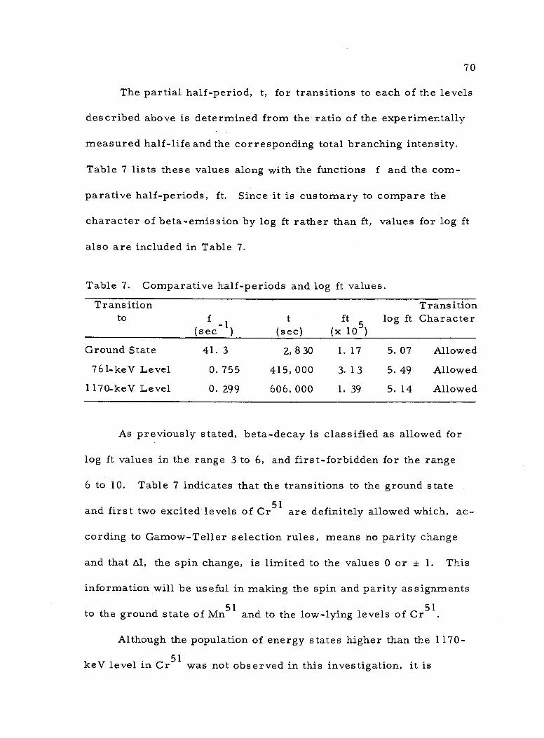
The partial half- period, t, for transitions to each of the levels
described above is determined from the ratio of the experimentally
measured half -life and the corresponding total branching intensity.
Table 7 lists these values along with the functions f and the com-
parative half- periods, ft. Since it is customary to compare the
character of beta -emission by log ft rather than ft, values for log ft
also are included in Table 7.
Table 7. Comparative half- periods and log ft values.
Transition Transition to f t ft log ft Character
(sec -1) (sec) (x 105)
Ground State 41.3 2, 8 30 1. 17 5. 07 Allowed
761 -keV Level 0. 755 415, 000 3. 1 3 5. 49 Allowed
1170 -keV Level 0. 299 606, 000 1. 39 5. 14 Allowed
As previously stated, beta -decay is classified as allowed for
log ft values in the range 3 to 6, and first -forbidden for the range
6 to 10. Table 7 indicates that the transitions to the ground state
and first two excited levels of Cr51 are definitely allowed which, ac-
cording to Gamow -Teller selection rules, means no parity change
and that AI, the spin change, is limited to the values 0 or f 1. This
information will be useful in making the spin and parity assignments
to the ground state of Mn51 and to the low -lying levels of Cr 51.
Although the population of energy states higher than the 1170-
keV level in Cr51 was not observed in this investigation, it is
71
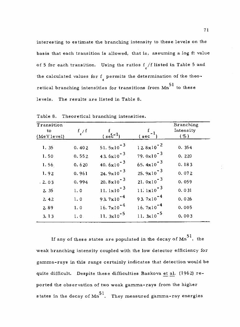
interesting to estimate the branching intensity to these levels on the
basis that each transition is allowed, that is, assuming a log ft value
of 5 for each transition. Using the ratios f /f listed in Table 5 and E
the calculated values for f permits the determination of the theo- E
retical branching intensities for transitions from Mn51 to these
levels. The results are listed in Table 8.
Table 8. Theoretical branching intensities.
Transition Branching to f f f f Intensity
(MeVlevel) E ( sec-1) ( sec'1) ( %)
1. 35 0.402 51.5x10 -3 12. 8x10 -2 O. 354
1.50 0.552 43.6x10⁻³ 79. 0x10- 3 O. 220
1.56 0.620 40.6x10⁻³ 65.4x10'3 0. 183
1.92 0.961 24.9x10'3 25.9x10 3 0. 07 2
2. 0 3 0 994 20. 8x10 -3 21. 0x10- 3
0. 059
2. 35 1. 0 11. 1x10- 3 11. 1x10- 0. 0 31
2.42 1.0 93.7x10 4 93.7x10 0.026
2.
3.
89
13
1.
1.
0
0
16.
11.
7x10⁻⁴
3x10⁻⁵
16.
11.
7x10⁻⁴
3x10⁻⁵
0.
0. 00 3
005
If any of these states are populated in the decay of Mn51, the
weak branching intensity coupled with the low detector efficiency for
gamma -rays in this range certainly indicates that detection would be
quite difficult. Despite these difficulties Baskova et al. (1962) re-
ported the observation of two weak gamma -rays from the higher
states in the decay of Mn51. They measured gamma -ray energies
72
of 1. 56 MeV and 2. 03 MeV which correspond to branching to the fifth
and seventh excited levels of Cr51, respectively. They also meas-
ured the relative intensities of these gamma -rays to be 1. 0 percent
and 0. 5 percent of the positons, respectively. Converting these
relative intensities to equivalent branching intensities and comparing
the results with the values in Table 8 indicates the intensity meas-
urements of Baskova et al. are an order of magnitude larger than
expected. In addition to this discrepancy, Baskova and co- workers
make no mention of observing the more intense 761 -keV and 1170 -
keV gamma -rays previously reported by Nozawa et al. (1960) and
also observed in this investigation.
Before establishing the spin and parity assignments for the de-
cay scheme of Mn51, the calculation of one additional parameter is
required, namely, the mean -life times of the 761 keV and 1170 -keV
levels of Cr51. These values of course depend upon knowing whether
the gamma- radiation is electric or magnetic multipole and the multi-
polarity of the emitted radiation which results from the decay of
these levels. Theoretical expressions for the mean -life times have
been formulated by Weisskopf (1951) and are written below. The
first expression gives the mean -life time for electric multipole radi-
ation while the second is for magnetic multipole radiation,
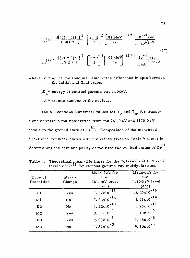
73
+
T() -.@(( 2.Q + 1) i 1 2 + 12[1:97 MeV at 1 10 -21 sec
e 4. 4(/ + 1) 3 E Y (1.`4Á/3.Q ) 2
(17)
2[(22 + 1)lt 2 .Q+3 2 197 MeV 2.Q + 1 sec
Tm(i) 1.9(.¢ + 1) 3 Ey 1/3 2.8-2 (1.4A )
where f = DI, is the absolute value of the difference in spin between the initial and final states,
E = energy of emitted gamma -ray in MeV, Y
A = atomic number of the nucleus.
Table 9 contains numerical values for Te e
and T m for transi-
tions of various multipolarities from the 761 -keV and 1170 -keV
levels to the ground state of Cr51. Comparison of the measured
life -times for these states with the values given in Table 9 assist in
determining the spin and parity of the first two excited states of Cr51.
Table 9. Theoretical mean -life times for the 761 -keV and 1170 -keV levels of Cr51 for various gamma -ray multipolarities.
Type of Transition
Parity Change
Mean -life for the
761 -keV level (sec)
Mean -life for the
1170 -keV level (sec)
El Yes 1. 17x10 -15 .3. 20x10 -16
M1 No 7. 33x10 -14 2. 01x10 -14
E2 No 1.52x10 -10 1.76x10 -11
M2 Yes 9. 50x10 -9 1. 10x10 -9
E3 Yes 2. 99x10 -5 1. 46x10 -6
M3 No 1. 87x10 -3 9.12x10 -5
L J L J `
=
L
74
The spin and parity of the ground state of Cr51 have been well
established as Z
in agreement with the shell model prediction for
the closed íf71 shell minus one configuration. Using atomic -beam 2
magnetic resonance techniques, Childs and co- workers (1959) meas-
ured the nuclear spin of Cr51 as 2
while Zeidman et al. (1960) de-
termined the parity from (d, t) reactions on Cr52. The latter investi-
gation determined the orbital angular momentum 2 of the odd neu- n
tron to be 3 with no mixture of .Q = 1, indicating the ground state to
be a pure 1f7, level.
For the purpose of comparing theory with experiment, the nu-
clear level structure with spin -orbit coupling, which is fundamental
in the description of the nuclear shell model, is illustrated in Figure
27 (Mayer and Jensen, 1955). The levels on the left, which do not
include the spin -orbit splitting, are intermediate between the levels
for a pure isotropic harmonic oscillator potential and those for an
infinite square well potential. Utilizing the concept of spin -orbit
coupling and the potential wells listed above, Maria Mayer was able
to formulate a nuclear model capable of explaining the "magic num-
bers". In addition to giving an adequate explanation of the magic
numbers, the nuclear shell model has been quite successful in pre-
dicting the spin and parity of the ground state of odd A nuclei, par-
ticularly for isotopes with nucleon numbers in the range 20 to 28.
Table 10 lists the proton and neutron configurations for odd A nuclei
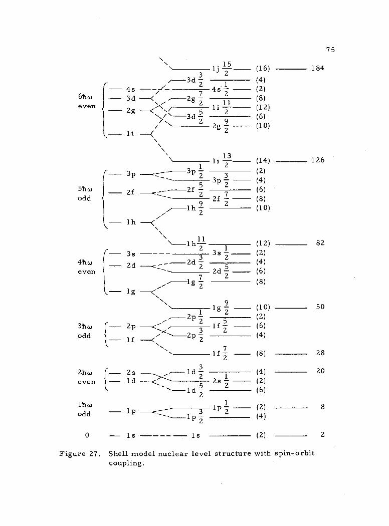
66i w
even
5Tico
odd
4t w
even
Thu) odd
2T-iou
even
1hw odd
0
Figure 27.
. \` 1 j Z (16)
i--3d 3 (4)
4s / 4s - (2) -2g 7 2
2g -- 5 li Zl (12)
3d 9
(6) 2g 2 (10)
1 i --- \
13 li 2 3p -_, p 2 3
3p 2f 5 2
1 h 9 2f
Z
2
2f
lh-{ \-1h2
3s 3s 2 2d 2d
5 - 2d 2 7
lg 2 1 g ---K
'N. N 9 lg
---/- 2p 2 5 (2) --<' / 1f - (6) _-2p 2 2 (4)
2p
lf
(- 2s
1
is
(14) (2) (4) (6) (8) (10)
(12) (2) (4) (6)
(8)
1 f 2 (8)
1 d 3 (4) 2 2s 1 (2)
1 d 5
2 (6)
3 lp (2) - 1p2 (4)
1 (2)
184
126
Shell model nuclear level structure with spin -orbit coupling.
82
50
28
20
8
2
75
3 -<\
N 2
2
1
\ i .
1
.. 1
1d -
(8)
(10)
- 2 -
- - - Í- - - -
- I - l
-
_ - -
--__-
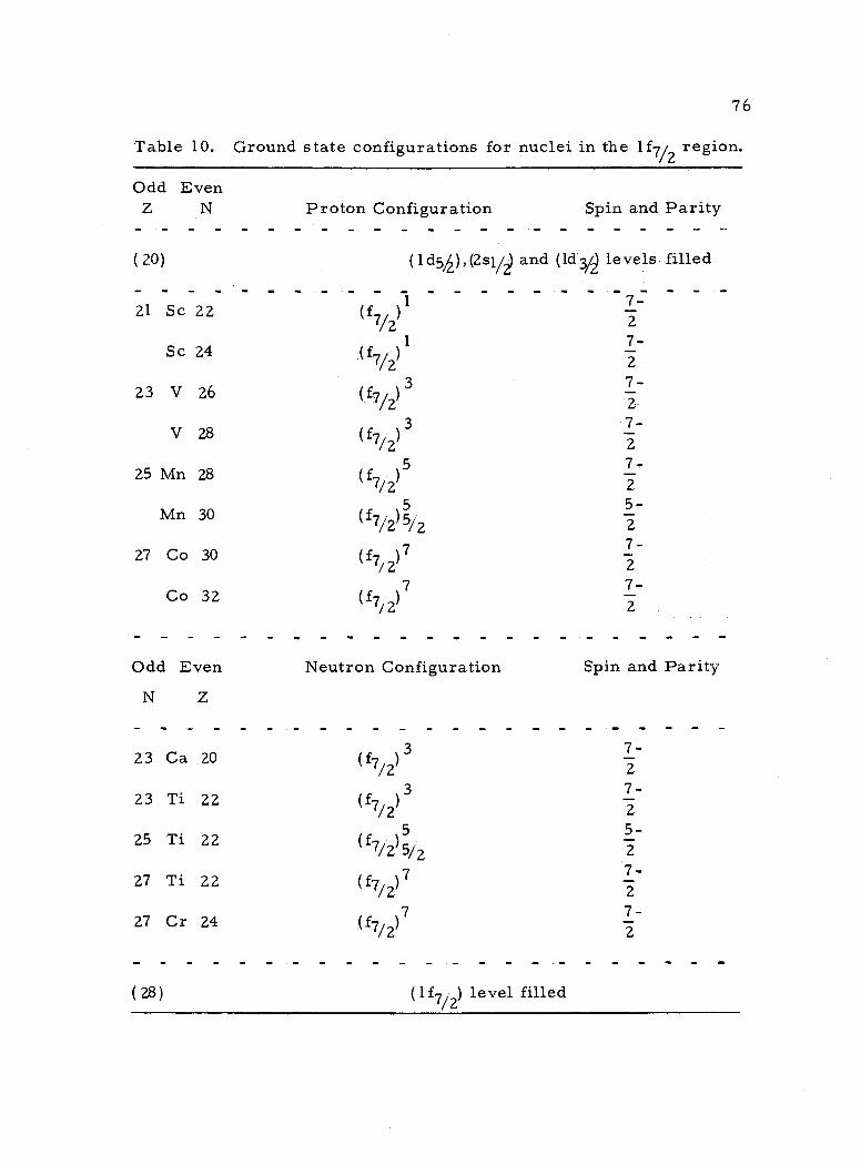
76
Table 10. Ground state configurations for nuclei in the 1f712 region.
Odd Even Z N
(20)
21 Sc 22
Sc 24
23 V 26
V 28
25 Mn 28
Mn 30
27 Co 30
Co 32
Proton Configuration Spin and Parity
(1 d51), (2s1,/ and (1d3/2 levels filled
- - - (f7/2)
- - -
1
(f72) 2
( fv2) 3 2 3 7-
(f7/2) 2 )5 7- 7/2 2
5 5- (f7/2)512 2
(f7/2)7 7- (f7/2)7
7 7- (f7/2) 2
Odd Even Neutron Configuration
N Z
23 Ca 20 (f712) 3
23
25
27
27
Ti 22
Ti 22
Ti 22
Cr 24
(f7/2) 3
(f7/2) /2 (f7/2)7
(f7/2) 7
( 28) (1f7/2) level filled
Spin and Parity
7- 2
7- 2
5- 2
7- 2
7- 2
7- 2
7-
7-
2
- - _ - - - - -
- _ _ _ - - - - - -
77
with proton and neutron numbers in the region 20 to 28 and the cor-
responding experimentally determined spin and parity assignments
for the ground states of these nuclei (Siegbahn, 1964). According to
Figure 27 the filling of the 1f7/2 level occurs in this region and one
expects, from the simple pairing shell model prediction, the ground
state spin and parity assignments for nuclei in this region to be 2'
With the exceptions of Mn55, Ti47, and perhaps Cr49, theory and
experiment agree. The latter isotopes, with 2
ground state con-
figurations, are classified as anomalies in the theory of the shell
model. An interesting observation is that all three isotopes have
either five protons or neutrons beyond the closed shell of 20 and that
the first two have two neutrons and protons, respectively, beyond
the closed shells of 28 and 20. The Cr49 isotope has four protons
beyond the closed shell of 20. However, Mn 53 with five protons be-
yond the closed shell of 20 and a closed neutron shell of 28 has a
measured 2-
ground state configuration which is consistent with the
shell model prediction. It appears that the coupling of the even nu-
cleon numbers beyond the closed shells destroys the expected 7- 2
single particle configuration in favor of the 2-
coupling for the odd
nucleon number five associated with the three anomalies listed above.
As yet, however, a satisfactory theoretical explanation of this phe-
nomenon does not exist.
On the basis of the simple pairing shell model one expects Mn51 51
.
78
to have a 2-
ground state spin and parity assignment, but on the
other hand, comparison with the three anomalies listed above, one
might predict a 2
ground state assignment since Mn51 has five pro-
tons beyond the closed shell of 20 and two neutron holes from the
closed shell of 28, a configuration similar to Ti47 assuming holes
and particles behave in the same manner. In the following discussion
5- arguments are given which support the assignment of 2
.
The log ft value for the decay of Mn51 to the ground state of
Cr51, calculated as 5. 07, certainly indicates this transition is al-
lowed. The 2 configuration for the Cr51 ground state and the
Gamow- Teller selection rules for allowed transitions restrict the
possible ground state assignment for Mn51 to the values
9- 2
5- 7- 2, 2, or
Kane and co- workers (1962) using thermal neutron capture in
Cr50 to study the level structure of Cr51 observed a strong 8. 499 -
MeV capture gamma -ray transition to the 761 -keV level of Cr51.
Using the following reasoning they concluded the capture gamma -ray
to have an El character:
From the systematics of capture -gamma -ray transition probabilities it is known that the great majority of strong, high -energy transitions have dipole character, chiefly El. Furthermore, in the region near A^-155 the energy of the 3s single -particle level is close to the neu- tron binding energy, so that strong El transitions are expected to occur between the state formed in neutron capture and low -lying p states of the residual nucleus. Experimentally, capture -gamma -ray spectra in this
2
79
region are characterized by exceptionally intense transi- tions to low -lying levels.
The Cr51 state formed by thermal neutron capture in the even -even
nucleus of Cr50 has the intrinsic spin and parity of the captured neu-
tron, that is, 2 + . Assuming the 8. 499 -MeV transition from this +
level to the 761 -keV level of Cr51 is El, the spin of the 761 -keV
level is either 2 or 3
2 since a spin change of one unit is associated
with El transitions. If the spin for the 761 -keV level is taken as 2 ,
then the 761 -keV transition to the Z
ground state must be either E3
or M3 since a spin change of three units is involved. The calculated
mean -life times for E3 and M3 transitions shown in Table 9 are ac-
curate within two orders of magnitude. Comparing the experimental-
ly determined 11 ± 1 nsec life -time for the 761 -keV level with the
calculated values reveals that both E3 and M3 transitions have mean-
life times that are much larger than the experimentally measured
value. For this reason, the 2 spin assignment to the 761 -keV level
is rejected. For a 2 spin assignment to the level, the 761 -keV
transition to the 2
ground state must be. either E2 or M2 since the
two levels differ by two units of spin. However, arguments given
below show that an M2 transition is parity forbidden and therefore
must be eliminated from consideration. Comparing the calculated
mean -life time for an E2 transition from this level with the experi-
mentally determined life -time shows good agreement and strongly
80
supports the 2
spin assignment to the 761 -keV level of Cr 51.
Since only f- and possibly p- orbitals are involved, the parity
for this level is odd and is in agreement with the assumption of the
El character of the 8. 499 -MeV capture gamma -ray. Additional
support is given by the log ft value of 5. 49 (Table 8) for the decay of
Mn51 to the 761 -keV level of Cr51, an allowed transition with no
parity change from the odd parity of the ground state of Mn51. It is
therefore concluded that the spin and parity assignment for the 761-
keV level of Cr51 is 3 .
2
On the basis that transitions from Mn51 to the 2
761 -keV
level and to the 2
ground state of Cr51 are both allowed, the spin
and parity assignment for the ground state of Mn51 can be only 2- ,
the result expected from the previous discussion.
The decay of Mn51 to the second excited state of Cr51 is al-
lowed with a log ft value of 5. 14 which means the 1170 -keV level of
Cr51 has a probable spin and parity of 2
, -2- , or 2
. Since cap-
ture gamma -rays from thermal neutron studies of Cr50 have not
been observed for the 1170 -keV level, the 2- assignment is re-
jected. The upper -limit for the mean -life of the 1170 -keV state is
consistent with the conclusion of a 2-
or spin and parity assign-
ment for this level.
In summary, the decay scheme of Mn51 has been studied ex-
perimentally yielding the following results:
2
2
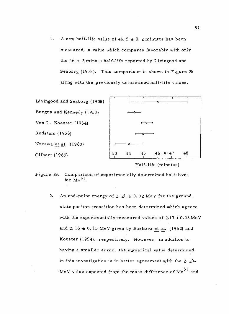
1. A new half -life value of 46. 5 f 0. 2 minutes has been
measured, a value which compares favorably with only
the 46 ± 2 minute half -life reported by Livingood and
Seaborg (1938). This comparison is shown in Figure 28
along with the previously determined half -life values.
Livingood and Seaborg (1938)
Burgus and Kennedy (1950)
Von L. Koester (1954)
Rudstam (1956)
Nozawa et al. (1960)
Glibert (1965)
81
o
43 44 45 46 F-o-+ 47 48
Half -life (minutes)
Figure 28. Comparison of experimentally determined half -lives for Mn51.
2. An end -point energy of 2. 21 ± 0. 02 MeV for the ground
state positon transition has been determined which agrees
with the experimentally measured values of 2.17 ± 0.05 MeV
and 2. 16 ± 0. 15 MeV given by Baskova et al. (1962) and
Koester (1954), respectively. However, in addition to
having a smaller error, the numerical value determined
in this investigation is in better agreement with the 2. 20-
MeV value expected from the mass difference of Mn51 and
82
Cr51 (Howard, 1963) than the two previously reported
end -point energies.
3. Gamma -ray energies of 761 ± 11 keV and 1170 ± 15 keV
and corresponding relative intensities of O. 70 ± O. 10 and
O. 48 ± O. 12 percent of the positons, respectively, have
been measured. The measured 1170 -keV gamma -ray
energy reported by Nozawa et al. (1960) agrees with the
value determined in this investigation. However, their
measured 740 -keV gamma -ray energy and the estimated
relative intensities of 0. 4 ± 0. 2 and 0. 2 ± 0. 1 do not
agree with the values determined here.
4. A mean -life time of 11 ± 1 nsec has been determined for
the 761 -keV level of Cr51 and an upper -limit of 1 nsec has
been given to the 1170 -keV level.
Combining these experimental results with theory, spin and
parity assignments were given to the low -lying levels of Cr51 and to
the ground state of Mn51. The ground state spin and parity as-
signment for Mn51 is not consistent with the 2
prediction of the
simple shell model theory and, therefore, Mn51 must be classified
as an anomaly along with the isotopes Mn55, Ti47 and Cr49.
Improvements are expected to be made in the measurements
reported in this investigation in the future with the advanced tech-
niques now being developed. First, enriched Cr50 targets
Z
83
(prohibitive cost for this investigation) should be used to reduce the
Mn54 contamination and any other impurities which might be present
as a result of bombarding natural chromium with deuterons. Second,
the gamma -ray energy measurements can be improved by using
high - resolution solid state detectors provided the detector efficiency
of the present models is increased. An attempt was made to use a
Li- drifted Ge- detector in this investigation to measure the gamma -
ray energies, but the extremely low detector efficiency did not re-
veal the low intensity 761 -keV and 1170 -keV gamma -rays. Similarly,
a solid state beta -ray detector could be used in the end -point energy
measurement provided it is capable of stopping high- energy positons
and its efficiency is increased. The presently available Li- drifted
Si- detectors have the undesirable effect of having a high- intensity
backscatter component in their response to monoenergetic electrons
a factor which cannot be tolerated in the investigation of continuous
beta -spectra. The limitations of the electronics in the measurement
of the mean -life time for the 1170 -keV level of Cr51 should be re-
moved in the future with the advances being made with fast solid state
circuitry.
84
BIBLIOGRAPHY
1. Bahn, E. L. et al. 1964. Decay of 20- minute Ag115. Physical Review 136:603 -617.
2. Baskova, K A. et al. 1962. Investigation of some radioactive nuclei in the region of the filled 1f712 shell. Soviet Physics, JETP 15:289-296.
3. Bauer, R. W. , J. D. Anderson and L. J. Christensen. 1963. Lifetimes of excited nuclear states using delayed- reaction gamma rays. Physical Review 130 :312 -319.
4. Beers, Yardley. 1957. Introduction to the theory of error. 2d ed. Reading, Massachusetts, Addison -Wesley. 66 p.
5. Berger, Martin J. and Stephan M. Seltzer. 1964. Tables of energy losses and ranges of electrons and positons. Washington, National Bureau of Standards. 1 27 p. (National Aeronautics and Space Administration, SP -3012)
6. Bertolini, G. , F. Cappellani and A. Rota. 1960. Corrections for backscattering and energy resolution in beta spectroscopy by scintillation detectors. Nuclear Instruments and Methods 9:107 -110.
7, Blatt, John M. and Victor F. Weisskopf. 1952. Theoretical nuclear physics. New York, Wiley. 864 p.
8. Bosch, H. E. and T. Urstein. 1963. Nuclear studies by means of beta spectroscopy with scintillation counters. Nuclear Instruments and Methods 24:109-1 21.
9. Bunker, M. E. and J. W. Starner. 1955. Decay of Ti51 and Cr51. Physical Review 97:1272 -1275.
10. Burgus, W. H. and J. W. Kennedy. 1950. Chemical effects accompanying the decay of Mn51. Journal of Chemical Physics 18:97 -105.
11. Childs, W. J. , L. S. Goudman and L. J. Kieffer. 1959. Nu- clear spin of Cr51. Bulletin of the American Physical_ Society 4:151.
85
1 2. Eisberg, Robert Martin. 1961. Fundamentals of modern physics. New York, Wiley, 729 p.
1 3. Evans, Robley D. 1955. The atomic nucleus. New York, McGraw -Hill. 97 2 p.
14. Everling, F. 1963. Mass and level systematics of 1f712 shell nuclei. Nuclear Physics 47:561 -583.
15. Feenberg, Eugene. 1955. Shell theory of the nucleus. Princeton, Princeton University Press. 211 p.
16. Freedman, M.S. et al. 1956. Correction for phosphor back - scattering in electron scintillation spectrometry. Review of Scientific Instruments 27 :716 -719.
17. Heath, R. L. 1964. Scintillation spectrometry gamma -ray spectrum catalogue. vol. 1. 2d ed. Washington. 264 p. (IDO- 16880 -1, AEC Research and Development Report, Physics, TID -4500 (31 st ed. ))
18. Hoel, Paul G. 1954. Introduction to mathematical statistics. 2d ed. New York, Wiley, 321 p.
19. Howard, Robert A. 1963. Nuclear physics. Belmont, Cali- fornia, Wadsworth. 578 p.
20. Johnson, R. G. , O. E. Johnson and L. M. Langer. 1956. Beta spectrum of C136. Physical Review 102:1142 -1148.
21. Kane, W. R. , N. F. Fiebiger and J. D. Fox. 1962. Coinci- dence studies of the thermal neutron capture gamma rays of chromium. Physical Review 125 :2037 -2048.
22. Kennett, T. J. and G. L. Keech. 1963. An anti -coincidence f3 -ray scintillation spectrometer. Nuclear Instruments and Methods 24 :142 -148.
23. Koester, Von L. 1954. Bestimmung der Zerfallsenergie einiger leichter Elemente mit Zählrohr- Absorptionsmethoden. Zeit- schrift für Naturforschung 9a:104-114.
24. Livingood, J. J. , F. Fairbrother and G. T. Seaborg. 19 37. Radioactive isotopes of manganese, iron, and cobalt. Physical Review 52:135.
86
25. Livingood, J. J. and G. T. Seaborg. 1938. Radioactive manga- nese isotopes. Physical Review 54:391-397.
26. Mayer, Maria Goeppert and J. Hans D. Jensen. 1955. Ele- mentary theory of nuclear shell structure. New York, Wiley. 269 p.
27. McCullen, J. D. , B. F. Bayman and Larry Zamick. 1964. Spectroscopy in the nuclear 1f7/2 shell. Physical Review 1 34 :515 -538.
28. Miller, D R. , R. C. Thompson and B. B. Cunningham. 1948. Products of high energy deuteron and helium ion bombardments of copper. Physical Review 74:347 -348.
29. National Research Council, Nuclear Data Group. 1955 et seq. Nuclear Data Sheets. Washington. various paging.
30. Nozawa, Masao, Hisashi Yamamoto and Yasukazu Yoshizawa. 1960. Search for weak gamma -rays in the positon decay of Mn51. Journal of the Physical Society of Japan 15:21 37-21 39.
31. Owen, G. E. and H. Primakoff. 1948. Relation between ap- parent shapes of monoenergetic conversion lines and of con- tinuous p - spectra in a magnetic spectrometer. Physical Review 74 :1406 -1412.
32. Owen, G. E. and H. Primakoff. 1950. Relation between ap- parent shapes of monoenergetic conversion lines and con- tinuous beta -spectra in a magnetic spectrometer. II. Review of Scientific Instruments 21 :447 -450.
33. Palmer, James P. and L. Jackson Laslett. 1950. Application of scintillation counters to beta -ray spectroscopy. Oak Ridge. 69 p. (United States Atomic Energy Commission, ISC -174)
34. Persson, B. 1964. An electron scintillation spectrometer. Nuclear Instruments and Methods 27 :1 -9.
35. Rose, M. E. 195 3. The analysis of angular correlation and angular distribution data. Physical Review 91 :610 -615.
36. Russell, H. T. 1960. Isolation of carrier -free Mn54 and I125
from cyclotron targets. Nuclear Science and Engineering 7 :323.
87
37. Schwarcz, Ervin H. 1963. Shell -model study of Mn55. Physical Review 129:727 -732.
38. Siegbahn, K. 1965. Alpha -, beta- and gamma -ray spectro- scopy. vol. 1. Amsterdam, North -Holland. 862 p.
39. Sommerfeldt, Raymond Walter. 1964. Perturbed directional correlation in Ta -181. Ph. D. thesis. Corvallis, Oregon State University. 110 numb. leaves.
40. U. S. Department of Commerce. 1952. Tables of the analysis of beta spectra. Washington. 61 p. (National Bureau of Standards, Applied Mathematics Series - 1 3)
41. Van_Patter, D. M. and S. M. Shafroth. 1964. Decay of 78. 4 h: Zr89 and 4. 18 min Zr89m. Nuclear Physics 50:11 3-1 35.
42. Wapstra, A. H. , G. J. Nijgh and R. Van Lieshout. 1959. Nu- clear spectroscopy tables. New York, Interscience. 135 p.
43. Weisskopf, V. F. 1951. Radiative transition probabilities in nuclei. Physical Review 8 3:107 3.
44. Zeidman, B. , J. L. Yntema and B. J. Raz. 1960. (d, t) reac- tions on nuclei with A 60. Physical Review 120:17 23 -17 30.
45. Zweifel, P. F. 1957. Allowed capture -positon branching ratios. Physical Review 107 :329 -330.

APPENDICES
88
APPENDIX I
SOURCE PREPARATION
Sources of Mn51 were produced from the Cr50(d, n) reaction by
bombarding natural chromium which contains 4. 31 percent Cr50
(Howard, 1963) with 7 -MeV deuterons provided by the Oregon State
University cyclotron. Chromium disks 10 mm diameter by 1 mm
thick were exposed for 15 minutes to a 20 µA beam of deuterons.
These disks were mounted on stainless steel backings which served
as water jackets for the cyclotron probe.
For the determination of the ground state positon end -point
51 energy, the Mn was removed from the target material after the
bombardment by a radiochemical process. The procedure followed
here was a carrier -free ion -exchange separation given by Russell
(1960) and is described in the following paragraph.
The exposed target material was first dissolved in a minimal
amount of 12N HC1 after which the solution was boiled to dryness.
To the resulting residue, 30 ml of five percent oxalic acid was
added and again the solution was boiled to dryness. This latter step
was repeated. After the evaporation process in the last step, 50 ml
of five percent oxalic acid was added to the residue and again was
heated to dissolve the solids. This solution was then filtered
89
through a 5 mm by 75 mm column of Dowex 50W -X4, 100 -200 mesh,
strongly acidic, cation exchange resin which had been activated with
five percent oxalic acid. In this process the manganese isotope re-
mains in the column of resin while the chromium and any other ele-
ments present pass through. The column was then washed with
100 ml of five percent oxalic acid to remove traces of chromium or
any additional elements. The oxalic acid was extracted from the
column by flushing with 100 ml of distilled water. To release the
manganese from the resin, 20 ml of O. 1N HC1 was passed through
the column. The solution was collected in a small beaker and was
heated if necessary to increase the specific activity. In most cases,
however, the specific activity was of sufficient strength that heating
was not necessary. The extraction of manganese by this method re-
quired approximately 60 minutes.
After this separation, the Mn51 was liquid- deposited on back-
ings of Au- mylar over an area of ,v0. 3 cm2 which previously
had been wetted with a dilute solution of insulin. Source thicknesses
of less than 100 µg /cm2 were obtained with this process.
90
APPENDIX II
WEIGHTED LEAST SQUARES FIT PROGRAM
It has been well established that the decay of a single radio-
active isotope follows the exponential decay law and that a graph of
the natural logarithm of the activity or the counting rate N(t) as a
function of time yields a linear curve which can be expressed by the
following equation.
ln N(t) = const. - X t (Al)
A measure of the slope of the decay curve gives the decay constant
A which is proportional to the half -life of the isotope.
The following discussion pertains to a description of the data
analysis in the half -life measurement of Mn51. In this analysis it
is desired to fit the relationship
1nN=a+bt (A2)
to a set of data points, in Ni, t., by the method of least squares in
which each data point is weighted inversely to the square of its stan-
dard deviation. The procedure followed here, developed by Rose
(1953), is to determine the parameters a and b which minimize the
expression
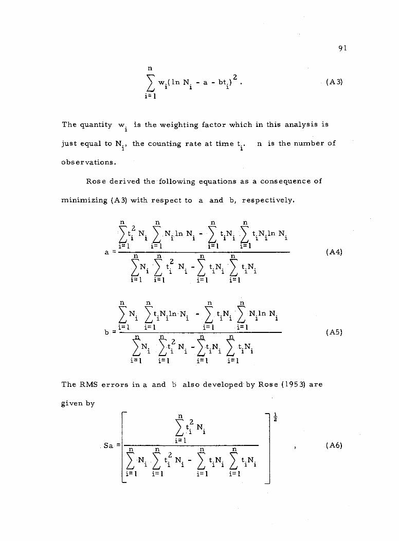
wi ( ln Ni - a - bt.) 2 .
i=1
91
(A3)
The quantity wi is the weighting factor which in this analysis is
just equal to N., the counting rate at time t.. n is the number of 1 1
observations.
Rose derived the following equations as a consequence of
minimizing (A3) with respect to a and b, respectively.
It? Ni N. ln Ni
i=1 i=1 a -
i=1 tiNi tiNiln
Ni i=1
n n n
N1 t? N1
t.N. 1
.i=1 i=1 i=1
t.N.1n N. i i 1
i=1 i=1
n
ti Ni. i=1
t.N. , N.ln N. 1 1 1 1
i=1
N n t2N-
n t.N. i i
n
tiNi i=1 i=1 i=1 l
The RMS errors in a and b also developed by Rose (195 3) are
given by
Sa -
n t? N. i 1
i=1
N. t. N. -
i=1 i=1
) t. N.
i=1
t.N.
i=1
i z
(A4)
(A5)
(A6)
n
- -
i i
Ni
b _i=1
-
i i i
r
)
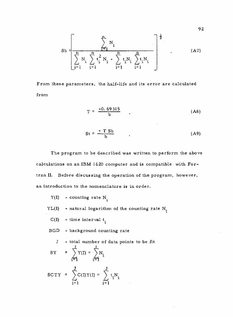
Sb -
i
92
(A7)
From these parameters, the half -life and its error are calculated
from
-0. 69 315 T
St - - T Sb b
(A8)
(A9)
The program to be described was written to perform the above
calculations on an IBM 1620 computer and is compatible with For-
tran II. Before discussing the operation of the program, however,
an introduction to the nomenclature is in order.
Y(I) - counting rate Ni
YL(I) - natural logarithm of the counting rate N, i
C(I) - time interval t.
BGD - background counting rate
J - total number of data points to be fit
SY -
i=
Y(I) =
SCTY = IC(I)Y(I) =
i=1 i=1
t.N. i i
i=1
n t. 2
N. - t. N. )'t.N. i=1 i=1
J
N
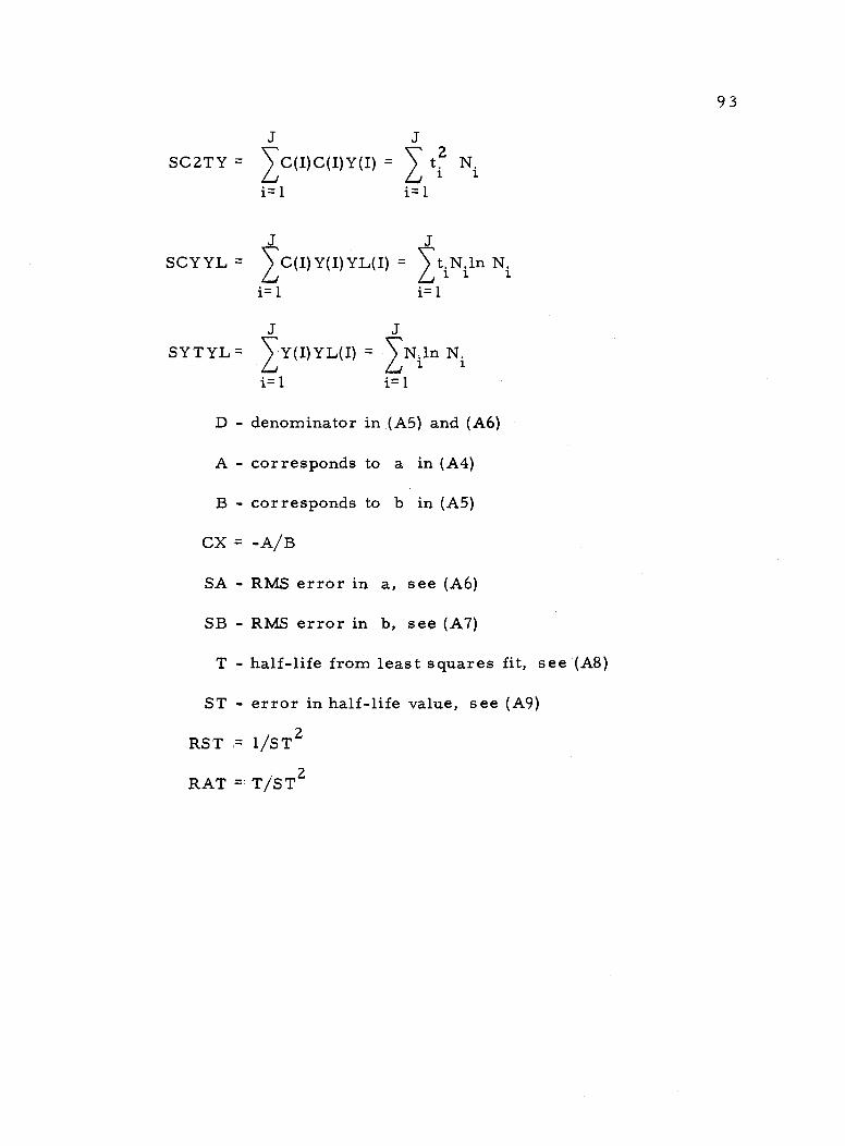
93
SC2TY =
SCYYL =
SYTYL=
J
IC(I)C(I)Y(I) = t2 Ni
i=1 i=1
IC(I) Y(I) YL(I) =
i=1
J Y(I)YL(I) =
i=1
J
i z 1
i=1
N.ln N. i 1
i=1
D - denominator in (A5) and (A6)
A - corresponds to a in (A4)
B - corresponds to b in (A5)
CX = -A /B
SA - RMS error in a, see (A6)
SB - RMS error in b, see (A7)
T - half -life from least squares fit, see (A8)
ST - error in half -life value, see (A9)
RST = 1 /ST2
RAT = T /ST2
J
J tiNiln Ni
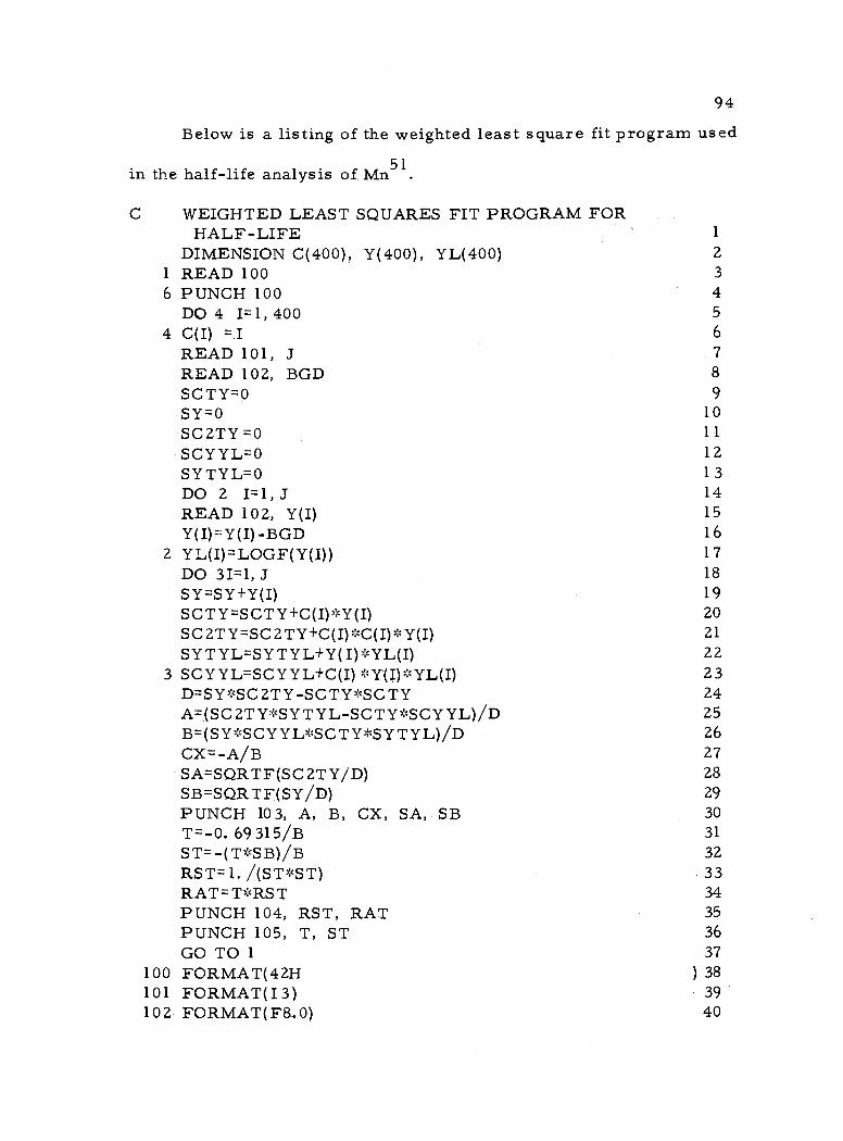
94
Below is a listing of the weighted least square fit program used
in the half -life analysis of Mn51.
C WEIGHTED LEAST SQUARES FIT PROGRAM FOR HALF -LIFE 1
DIMENSION C(400), Y(400), YL(400) 2
1 READ 100 3
6 PUNCH 100 4 DO 4 I =1, 400 5
4 C(I) =:I 6
READ 101, J 7
READ 102, BGD 8
SCTY =O 9
SY =O 10
SC2TY =0 11
SCYYL =O 12 SYTYL =O 13 DO 2 I =1, J 14 READ 102, Y(I) 15
Y(I)= Y(I) -BGD 16 2 YL(I)= LOGF(Y(I)) 17
DO 31=1, J 18
SY= SY +Y(I) 19
SCTY=SCTY+C(I)*Y(I) 20 SC2TY=SC2TY+C(I)*C(I)*Y(I) 21
SYTYL= SYTYL *YL(I) 22 3 SCYYL = SCYYL *YL(I) 23
D=SY'a°SC2TY-SCTY*SCTY 24 A= (SC2TY *SYTYL- SCTY *SCYYL) /D 25 B=(SYJ°SCYYL*SCTY'4SYTYL)/D 26 CX=-A/B 27 SA= SQRTF(SCZTY /D) 28 SB= SQRTF(SY /D) 29 PUNCH 103, A, B, CX, SA, SB 30 T = -0. 69 315/B 31
ST=- (T*SB) /B 32 RST =1. /(ST *ST) 33 RAT=T*RST 34 PUNCH 104, RST, RAT 35 PUNCH 105, T, ST 36 GO TO 1 37
100 FORMAT(42H ) 38 101 FORMAT(I3) 39 102 FORMAT(F8.0) 40
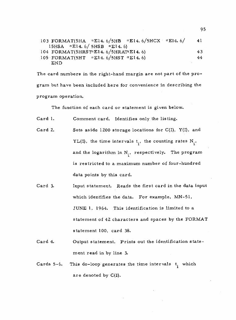
95
103 FORMAT(SHA = E14.6 /5HB = E14.6 /5HCX =E14.6/ 41 15HSA =E14. 6/ 5HSB =E14. 6)
104 FORMAT(5HRST=E14. 6/5HRAT=E14. 6) 43 105 FORMAT(5HT =E14. 6 /5HST =E14.6) 44
END
The card numbers in the right -hand margin are not part of the pro-
gram but have been included here for convenience in describing the
program operation.
The function of each card or statement is given below.
Card 1.
Card 2.
Card 3.
Card 4.
Cards 5 -6.
Comment card. Identifies only the listing.
Sets aside 1200 storage locations for C(I), Y(I), and
YL(I), the time intervals t., the counting rates N.,
and the logarithm in Ni, respectively. The program
is restricted to a maximum number of four -hundred
data points by this card.
Input statement. Reads the first card in the data input
which identifies the data. For example, MN -51,
JUNE 1, 1964. This identification is limited to a
statement of 42 characters and spaces by the FORMAT
statement 100, card 38.
Output statement. Prints out the identification state-
ment read in by line 3.
This do -loop generates the time intervals t, which
are denoted by C(I).
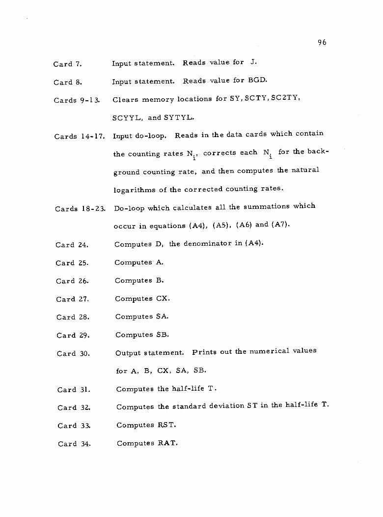
96
Card 7. Input statement. Reads value for J.
Card 8. Input statement. Reads value for BGD.
Cards 9 -1 3. Clears memory locations for SY, SCTY, SC2TY,
SCYYL, and SYTYL.
Cards 14 -17. Input do -loop. Reads in the data cards which contain
the counting rates ., corrects each N. for the back-
ground counting rate, and then computes the natural
logarithms of the corrected counting rates.
Cards 18 -23. Do -loop which calculates all the summations which
occur in equations (A4), (A5), (A6) and (A7).
Card 24. Computes D, the denominator in (A4).
Card 25. Computes A.
Card 26. Computes B.
Card 27. Computes CX.
Card 28. Computes SA.
Card 29. Computes SB.
Card 30. Output statement. Prints out the numerical values
for A, B, CX, SA, SB.
Card 31. Computes the half -life T.
Card 32. Computes the standard deviation ST in the half -life T.
Card 33. Computes RST.
Card 34. Computes RAT.
). i
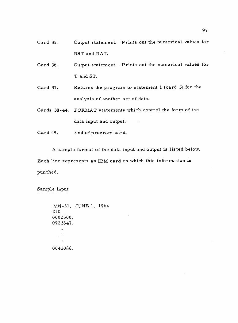
97
Card 35. Output statement. Prints out the numerical values for
RST and RAT.
Card 36. Output statement. Prints out the numerical values for
T and ST.
Card 37. Returns the program to statement 1 (card 3) for the
analysis of another set of data.
Cards 38 -44. FORMAT statements which control the form of the
data input and output.
Card 45. End of program card.
A sample format of the data input and output is listed below.
Each line represents an IBM card on which this information is
punched.
Sample Input
MN -51, JUNE 1, 1964 210 0002500. 0923547.
0043066.
98
Sample Output
JUNE 1, 1964 00
MN-51, A = 13.770985E B =-14.905720E-03 CX = 92. 387251E 01 SA = 19. 912163E-05 SB = 26. 283498E-07 RST = 14. 872743E 03 RAT = 69. 161648E 04 T = 46. 502282E 00 ST = 81.998226E-04
With the results provided by this program, the average values
of the half -life and the standard deviation were obtained from the
following relations (Beers, 1957).
J T./ST)
i-1 T = (A10)
J
J
/STi2 )
L(Ti -111(1/ST3. )
ST- i=1
(1 /ST2)
i=1
(All)
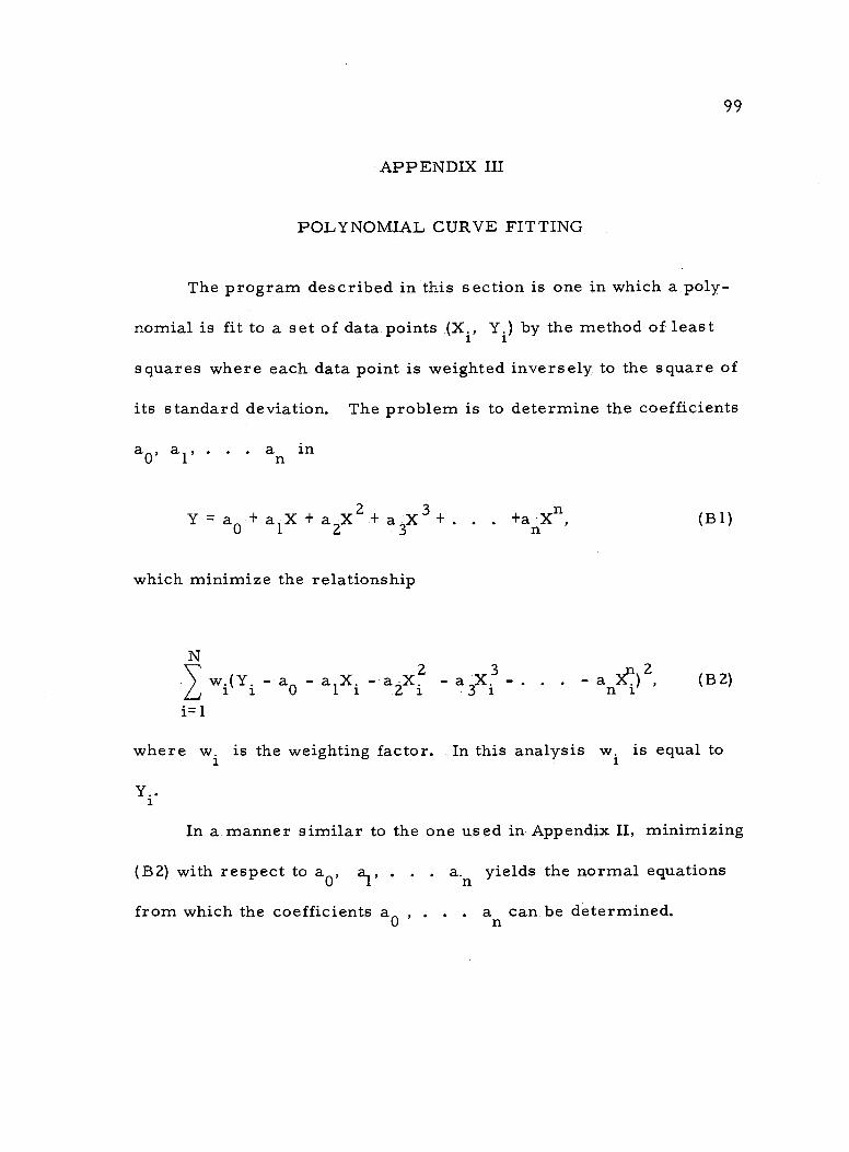
99
APPENDIX III
POLYNOMIAL CURVE FITTING
The program described in this section is one in which a poly-
nomial is fit to a set of data points (X., Y,) by the method of least
squares where each data point is weighted inversely to the square of
its standard deviation. The problem is to determine the coefficients
a0, al, . . . an in
Y = a0 +a1X +a2X2+a3X3+. . . +ariXn,
which minimize the relationship
(B1)
N
w.(Y. - a - a X. - a X? - a X3-. . . - a Xn)2, (B2) i 0 1 i 2 i 3 i n i=1
where wi is the weighting factor. In this analysis wi is equal to
Y.. i In a manner similar to the one used in Appendix II, minimizing
(B2) with respect to a0, al, a. n yields the normal equations
from which the coefficients a0 , . . . an can be determined.
1 1
1
.
i=1
N
+ a N N
w.X. + . . . + a ) w.Xn i i n
i=1 i=1
N
wiXi + a 1 wiX 2
+ . . + an
i=1 i=1
N
N
N w.Y.
i=1
w.X. + 1=
w1 Y1X1 (B3)
100
i=1 i=1
N N
wiXi + a wiXi + F. + 2n
= 1w. 3.
i=1 i=1 i=1 i=1
The function of this program written in Fortran II for an IBM
1620 computer is to solve the above set of simultaneous equations
for the coefficients a0, al, . . . an, and once these are deter-
mined, to calculate new values of Y. for each X. from (B1). The
data input for this polynomial curve fit is limited to a maximum of
250 points (X., Y.) to which a polynomial with a degree as high as
nine can be fit.
The program begins by finding the best straight line that fits
the data. It then fits successively higher order polynomials until
the order designated in the input by LAST is reached, or until the
value of the standard error of the polynomial fitted is less than TOL,
the allowable value of the standard error. When either of these
conditions is met, the coefficients a0, al, . . . an and the
¡ 1
N
1
1 1
wiX
1 1
N
a0
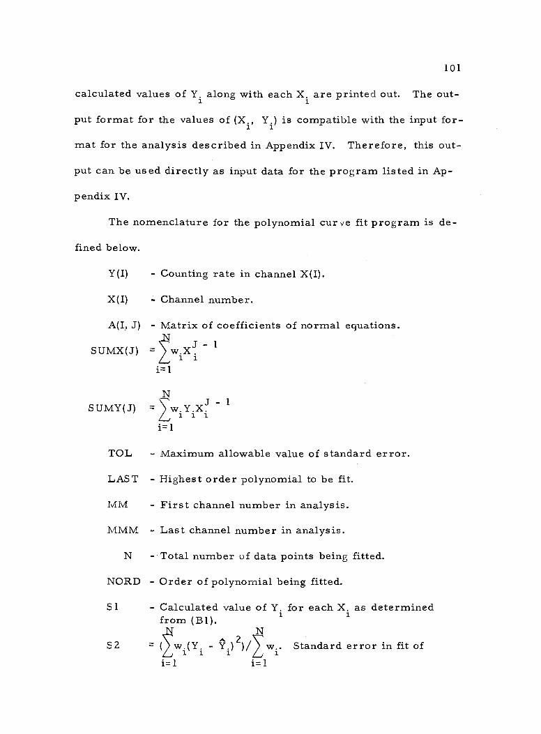
101
calculated values of Yi along with each Xi are printed out. The out-
put format for the values of (X., Y. is compatible with the input for- 1)
mat mat for the analysis described in Appendix IV. Therefore, this out-
put can be used directly as input data for the program listed in Ap-
pendix IV.
The nomenclature for the polynomial curve fit program is de-
fined below.
Y(I) - Counting rate in channel X(I).
X(I) - Channel number.
A(I, J) - Matrix of coefficients of normal equations.
SUMX(J) w.XJ - 1
i i i=1
SUMY(J) _ > w. Y.XJ - 1
i= 1
TOL - Maximum allowable value of standard error.
LAST - Highest order polynomial to be fit.
MM - First channel number in analysis.
MMM - Last channel number in analysis.
N - Total number of data points being fitted.
NORD - Order of polynomial being fitted.
S 1 Calculated value of Y. for each X. as determined from (B1).
N N S2 = (, wi(Y. - Y.)2)/ w Standard error in fit of
i=1 i=1
N
-
s
102
polynomial. Here Yi denotes the observed counting rate and Y, is the calculated value. i
S 3 = Y. - Y.. Difference between observed and calculated 3. counting rates.
Below is a listing of the polynomial curve fit program. Again,
as in Appendix II, each line or card has been given a number only
for convenience in describing the program operation.
C POLYNOMIAL CURVE FIT PROGRAM 1
DIMENSION X( 250), Y(250), A(10, 10), SUMX(19), SUMY(10) 2 1 READ 5 3
READ 2, TOL, LAST 4 2 FORMAT(E10. 4, 15) 5
PUNCH 5 6
5 FORMAT( 35H IDENTIFICATION OF CURVE ) 7
READ 22, MM, MMM 8
22 FORMAT(2I5) 9
N= MMM -MM +1 10 DO 40 I =1, N 11
20 READ 21, Y(I) 12 21 FORMAT(F8. 0) 1 3
X(I)= MM +I -1 14 40 CONTINUE 15
70 SUMX(1) =0. 16 SUMX(2) =0. 17 SUMX( 3) =0. 18 SUMY(1) =0. 19 SUMY(2) =0. 20 DO 90 I =1, N 21
SUMX(1)= SUMX(1) +1. /Y(I) 22 SUMX(2) =SUMX(2) +X(I) /Y(I) 23 SUMX( 3) =SUMX( 3) +X(I) *X(I) /Y(I) 24 SUMY(1) =SUMY(1) +1. 25
90 SUMY(2) =SUMY(2) +X(I) 26 NORD =1 27
9 3 L= NORD +1 28 KK =L +1 29 DO 101 I =1, L 30 DO 100 J =1, L 31
IK =3-1 +I 32 100 A(I, J) =SUMX(IK) 33
-
103
101 A(I, KK)=SUMY(I) 34 DO 140 I=1, L 35
A(KK, I)=-1. 36 KKK=I+1 37 DO 110 J=KKK, KK 38
110 A(KK, J)=0. 39
SS=1. /A(1, I) 40 DO 120 II= 2, KK 41 DO 120 J=KKK, KK 42
1 20 A(II, J)=A(II, J)-A(1, J)*A(II,,IPSS 43 DO 140 II41, L 44 DO 140 J=KKK, KK 45
140 A(II, J)=A(II+1, J) 46 S2=0. 47 DO 160 J=1, 1V' 48 51=0. 49 S1=S1+A(1, KK) 50 DO 150 I=1, NORD 51
150 S 1=S 1+A(I+1, KK)*X(J)**I 52 160 S2=S2+(S1-Y(J))*(S1-Y(J))/Y(J) 53
B=SUMX(1) 54 S2=(S2/B)**. 5 55
161 IF(NORD-LAST)162, 163, 162 56 162 IF(S2-TOL)163, 163. 171 57 163 PUNCH 41, NORD, TOL,.S2, N 58
41 FORMAT(I 3, 15H ORDER EQUATION/ 10HTOLERANCE =E14. 7/ 59
115HSTANDARD ERROR=E14. 7/2HN=15/) 60 DO 164 I=1, L 61 J=I-1 62
164 PUNCH 42, J, A(I, KK) 63 42 FORMAT(1HAI2 1H=E14. 7) 64
165 IF(NORD-LAST)166 167, 166 65 166 IF(S 2-TOL)167, 167, 171 66 167 DO 169 I=1, N 67
51=0. 68 S 1=A(1, KK) 69 DO 168 J=1, NORD 70
168 S 1=S 1+A(J+1, KK)*X(I)**J 71
S 3=Y(I)-S 1 72 169 PUNCH 43, X(I), Y(I), Si, S3 73 43 FORMAT(E10. 3, 3XE14. 7, 3XE14. 7, 3XE14. 7) 74
112 IF(NORD-LAST) 170, 173, 173 75 170 IF(S2-TOL)173, 173, 171 76 171 NORD=NORD+1 77
104
J= 2*NORD 78 SUMX(J)=0. 79 SUMX(J+1)=0. 80 SUMY(NORD+1)=0. 81 DO 172 I=1, N 82 SUMX(J)=SUMX(J)+(X(I)**(J-1))/Y(I) 83 SUMX(J+1)=SUMX(J+1)+(X(I)**J)/Y(I) 84
172 SUMY(NORD+1)=SUMY(NORD+1)+X(I) **NORD 85 GO TO 93 86
173 P=1. 87 GO TO 1 88 END 89
The function of each card or group of cards in the operation of
this program is discussed below.
Card 1. Comment card. Identifies only the program listing.
Card 2. Dimension statement. Provides memory locations
for X(I), Y(I), A(I, J), SUMX(I), and SUMY(I).
Card 3. Input statement. Reads in identification statement,
for example, MN -51, JUNE 1, 1964. This statement
is limited to 35 characters including spacing.
Card 4. Input statement. Reads in TOL and LAST.
Card 5. Format statement. Establishes the form of the input
for TOL and LAST.
Card 6. Output statement. Prints out statement read in by
card 3.
Card 7. Format statement for input and output from cards 3
and 5, respectively.
105
Card 8. Input statement. Reads in MM and MMM, the first
and last channel numbers in the analysis, respectively.
Card 9. Format statement for input of MM and MMM.
Card 10. Calculates the total number of data points using the
first and last channel numbers.
Cards 11 -15. Do -loop in which the counting rates Y(I) are read in
and the corresponding channel numbers X(I) are cal-
culated. The Format statement is for the Y(I) input.
Cards 21 -26. Calculate the summations present in the normal equa-
tions when a first order polynomial is fit. The addi-
tional summations which are required in the fit of
higher order polynomials are calculated by cards
82 -85.
Card 27. Establishes the order of the polynomial to be fit as
unity.
Cards 28 -29. Establishes values for the control parameters L and
KK.
Cards 30-34. Do -loop in which the matrix of coefficients of normal
equations is calculated.
Cards 35 -46. Do -loop in which the a0, al, a2 . . . an coefficients
in the normal equations are determined.
Card 47. Clears the memory location for S2.
Cards 48 -55. Do -loop which calculates the standard error S2.
106
Card 56. Compares NORD the order of the polynomial being
fitted with the highest order specified by LAST in the
input. If NORD is not equal to LAST, the program
continues to the next statement on card 57. If NORD
is equal to LAST, however, the program skips card
57 and proceeds to card 58.
Card 57. Compares the calculated standard error 52 with the
maximum allowable error TOL specified in the input.
If SZ is less than or equal to TOL, then the program
is directed to card 77, statement 171, where the
calculations for the fit of the next higher order poly-
nomial begins.
Cards 58 -74. Output statements. The values for NORD, TOL, S2,
N, the coefficients a0, al, a2, . . an in the normal
equations (B3), each channel number X(I) along with
the observed counting rate Y(I) and the calculated
counting rate SI, and S3 the difference between
Y(I) and S1 are printed out.
Cards 75 -76. Control statements. If the program passes through
cards 58 -74, then cards 75 and 76 transfer the pro-
gram to card 87. Otherwise, the program proceeds
to card 77.
.
107
Cards 77 -86. Calculate the additional summations required for the
fit of the next higher order polynomial and then trans-
fer the program back to card 28.
Cards 87 -88. Transfer program to card 3 where a new set of data
can be read in and analysed.
Card 89. End statement required for compiler control.
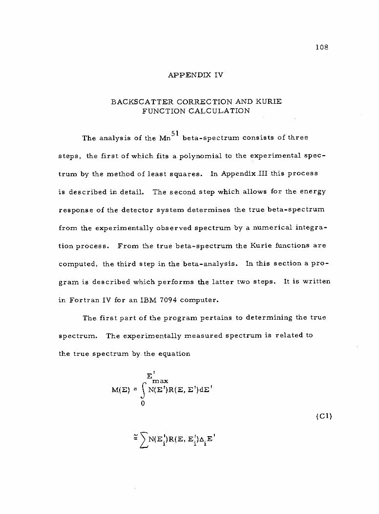
108
APPENDIX IV
BACKSCATTER CORRECTION AND KURIE FUNCTION CALCULATION
The analysis of the Mn51 beta -spectrum consists of three
steps, the first of which fits a polynomial to the experimental spec-
trum by the method of least squares. In Appendix III this process
is described in detail. The second step which allows for the energy
response of the detector system determines the true beta -spectrum
from the experimentally observed spectrum by a numerical integra-
tion process. From the true beta- spectrum the Kurie functions are
computed, the third step in the beta -analysis. In this section a pro-
gram is described which performs the latter two steps. It is written
in Fortran IV for an IBM 7094 computer.
The first part of the program pertains to determining the true
spectrum. The experimentally measured spectrum is related to
the true spectrum by the equation
E max M(E) SN(E')R(E,E')dE'
0
N(Ei)R(E,
(Cl)
Ei)oiEt
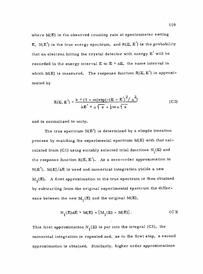
109
where M(E) is the observed counting rate at spectrometer setting
E, N(E') is the true energy spectrum, and R(E, E') is the probability
that an electron hitting the crystal detector with energy Et will be
recorded in the energy interval E to E + 6E, the same interval in
which M(E) is measured. The response function R(E, Et) is approxi-
mated by
R(E, E k + (1 - m)exp(-(E - E')2 a2)
kE + a, - im a fri- (C2)
and is normalized to unity.
The true spectrum N(E') is determined by a simple iteration
process by matching the experimental spectrum M(E) with that cal-
culated from (Cl) using suitably selected trial functions Ni (E) and
the response function R(E, E'). As a zero -order approximation to
N(E'), M(E) / ©E is used and numerical integration yields a new
M1(E). 1
A first approximation to the true spectrum is then obtained
by subtracting from the original experimental spectrum the differ-
ence between the new M1(E) and the original M(E),
N1(E)AE = M(E) - [M1(E) - M(E)] . (C3)
This first approximation N1(E) is put into the integral (Cl), the
numerical integration is repeated and, as in the first step, a second
approximation is obtained. Similarly, higher order approximations
- n
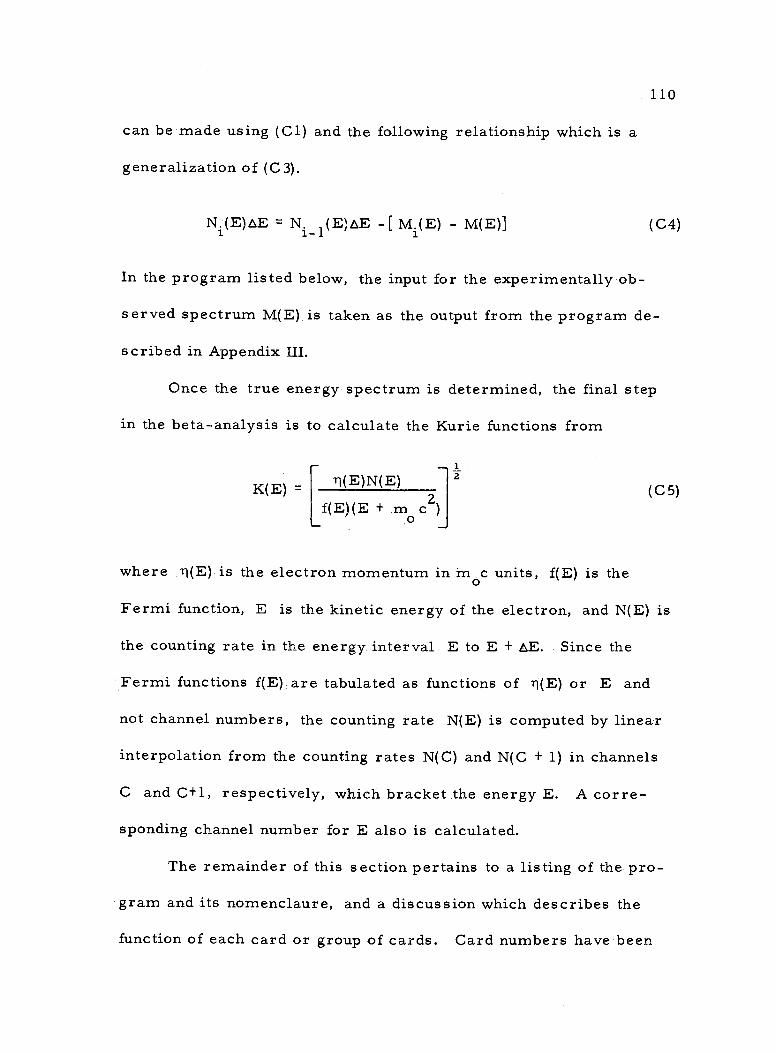
110
can be made using (C1) and the following relationship which is a
generalization of (C 3).
Ni(E)®E - Ni-1(E)AE -L Mi(E) - M(E)] (C4)
In the program listed below, the input for the experimentally ob-
served spectrum M(E) is taken as the output from the program de-
scribed in Appendix III.
Once the true energy spectrum is determined, the final step
in the beta -analysis is to calculate the Kurie functions from
K(E) r1(E)N(E)
f(E)(E + m c2) 0
(C5)
where (E) is the electron momentum in. in c units, f(E) is the 0
Fermi function, E is the kinetic energy of the electron, and N(E) is
the counting rate in the energy interval E to E + tE. Since the
Fermi functions f(E) are tabulated as functions of n(E) or E and
not channel numbers, the counting rate N(E) is computed by linear
interpolation from the counting rates N(C) and N(C + 1) in channels
C and C +1, respectively, which bracket the energy E. A corre-
sponding channel number for E also is calculated.
The remainder of this section pertains to a listing of the pro-
gram and its nomenclaure, and a discussion which describes the
function of each card or group of cards. Card numbers have been
_ I
_
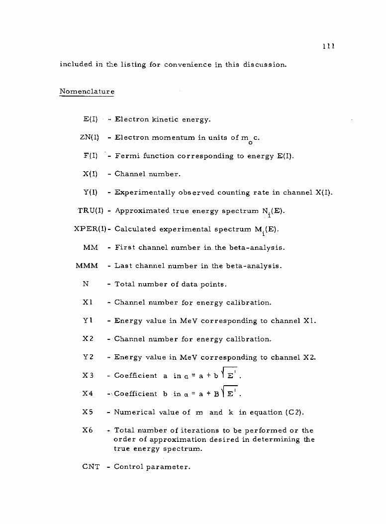
111
included in the listing for convenience in this discussion.
Nomenclature
E(I) Electron kinetic energy.
ZN(I) Electron momentum in units of m c. o
F(I) - Fermi function corresponding to energy E(I).
X(I) - Channel number.
Y(I) - Experimentally observed counting rate in channel X(I).
TRU(I) - Approximated true energy spectrum Ni(E).
XPER(I)- Calculated experimental spectrum Mi (E).
MM - First channel number in the beta -analysis.
MMM - Last channel number in the beta -analysis.
N - Total number of data points.
X1 - Channel number for energy calibration.
Y1 - Energy value in MeV corresponding to channel X1.
X2 - Channel number for energy calibration.
Y2 - Energy value in MeV corresponding to channel X2.
X 3 - Coefficient a in a= a + b I E .
X4 Coefficient b in a= a + B fET.
X5 - Numerical value of m and k in equation (C2).
X6 Total number of iterations to be performed or the order of approximation desired in determining the true energy spectrum.
CNT - Control parameter.
-
-
-
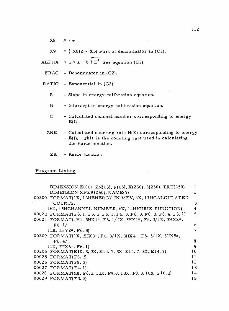
112
X8 = 1
X9 = 2 X8(2 of denominator in (C2). ; ALPHA = a = a + b 1 E See equation (C2).
FRAC - Denominator in (C2).
RATIO - Exponential in (C2).
R - Slope in energy calibration equation.
B - Intercept in energy calibration equation.
C - Calculated channel number corresponding to energy E(I).
ZNE - Calculated counting rate N(E) corresponding to energy E(I). This is the counting rate used in calculating the Kurie function.
ZK - Kurie function
Program Listing
DIMENSION E(66), ZN(66), F(66), X(250), 6(250), TRU(250) 1
DIMENSION XPER(250), NAME(7) 2
00200 FORMAT(1X, 1 3HENERGY IN MEV, 6X, 17HCALCULATED COUNTS, 3
16X, 15HCHANNEL NUMBER, 6X, 14HKURIE FUNCTION) 4 00023 FORMAT(F6. 1, F6. 3, F6. 1, F6. 3, F6. 3, F6. 3, F6. 4, F6. 1) 5
00024 FORMAT(1H1, 3HX1=, F6. 1/1X, 3HY1=, F6. 3/1X, 3HX2=, F6. 1/ 6
11X, 3HY2=, F6. 3) 7
00209 FORMAT(1X, 3HX3=, F6. 3/1X, 3HX4=, F6. 3/1X, 3HX5=, F6. 4/ 8
11X, 3HX6=, F6. 1) 9 00206 FORMAT(E10. 3, 3X, E14. 7, 3X, E14. 7, 3X, E14. 7) 10 00025 FORMAT(F6. 3) 11
00026 FORMAT(F8. 3) 12 00027 FORMAT(F4. 1) 13 00028 FORMAT(5X, F6.3, 13X, F9.0, 13X, F8.3, 10X, F10.3) 14 00029 FORMAT( F 3. 0) 15
X5) Part

113
00022 FORMAT( 2I5) 16
00043 FORMAT(E10. 3, 20X, E14. 7) 17 00502 FORMAT( 7A5) 18
00602 FORMAT( 1H , 7A5) 19 READ( 5, 27)(Z.N(I), I=1, 66) 20 READ(5, 25)(E(I), I=1, 66) 21
00500 READ(5, 26)(F(I), I=1, 66) 22 0050 3 READ( 5, 502)NAME 2 3
WRITE(6, 602)NAME 24 READ( 5, 22)MM, MMM 25 N=MMM-MM+1 26
00173 READ(5, 23)X1, Y1, X2, Y2, X3, X4, X5, X6 27 WRITE(6, 24)X1, Y1, X2, Y2 28
WRITE( 6, 209)X 3, X4, X5, X6 29 READ(5, 43)(X(I), Y(I), I=1, N) 30
READ(5, 29)CNT 31
PI= 3. 14159 32
X8=SQRT(PI) 33 X9=X8*(2. -X5)/2. 34 DO 2 I=1, N 35
00002 TRU(I)=Y(I) 36
LL=X6 37
DO 3 L=1, LL 38 00 304 DO 4 I 1, N 39
00004 XPER(I)=0. 40 DN=X(N) 41
ALPHA=X 3+X4*(SQRT(DN)) 42 XPER(N)=(X5,;,TRU(N))/(X5*DN+X9*ALPHA) 43 K=N-1 44 DO 20 I=1, K 45 J=N-1 46 DJ=X(J) 47 ALPHA=X 3+X4 *(SQRT(DJ)) 48
00201 XPER(J)-XPER(J+1)+(X5*TRU(J))/(X5*DJ+X9-,°ALPHA) 49 DO 400 I=1, N 50 DI=X(I) 51
ALPHA=X3+X4*(SQRT(DI)) 52 00400 XPER(I)=XPER(I)+(1. -X5)*(TRU(I))/(X59tiDI+X9*ALPHA) 53
DO 401 I=1, N 54 DI=X(I) 55 ALPHA=X 3+X4*(SQRT(DI)) 56 FRAC=1. /(X 5*DI+X9-,°ALPHA) 57 JJ= 3. *ALPHA 58 DO 401 J=1, JJ 59 DIFF=J 60
-
114
JJJ=I+J 61
RATIO=DIFF*DIFF/(ALPHA *ALPHA) 62 GAUSS=1. /(EXP(RATIO)) 6 3
J1=I-J 64 J2=I+J 65 IF(I-J)403, 403, 402 66
00402 XPER(J1)=XPER(J1)+FRAC*(1. -X5)*GAUSS*TRU(I) 67 00403 IF(JJJ. GT. MMM)GO TO 401 68 00404 XPER(J2)=XPER(J2)+FRAC*GAUSS *TRU(I) 69 00401 CONTINUE 70
DO 205 I=1, N 71
00205 TRU(I)=TRU(I)-XPER(I)+Y(I) 72 00202 WRITE(6, 206)(X(I), TRU(I), Y(I), XPER(I), I=1, N) 73
WRITE(6, 200) 74 R=(Y2-Y1)/(X2-X1) 75 B=Y2-R*X2 76 DO 3 I=1, 66 77 C=(E(I)-B)/R 78 FINAL= MMM 79 ZZ=MM 80 IF(ZZ. GT. C)GO TO 3 81
00008 IF(C. GT. FINAL)GO TO 3 82 00210 NLOW=C 83
GLO W=NLO W 84 NLO W=NLOW-MM+1 85 NUP=NLOW+1 86 ZNE=TRU(NLOW)+(C-GLOW)*(TRU(NUP)-TRU(NLOW)) 87 ZK=SQRT( ZN(I)*ZNE/(F(I) *(E(I)+ . 511E+00))) 88 WRITE(6, 28)E(I), ZNE, C, ZK 89
00003 CONTINUE 90 IF(CNT-2. )503, 500, 501 91
00501 STOP 92 END 93
The following specifies the function of each card or group of
cards in the program listed above.
Cards 1 -2. Dimension statements. Provide adequate memory
locations for E(I), ZN(I), F(1), X(I), Y(I), TRU(I),
XPER(I), and NAME.
-
115
Cards 3 -19. Format statements. Establish form of input and out-
put parameters, and provide captions for data output.
Card 20. Input statement. Reads in 66 tabulated values of the
electron momentum ZN(I).
Card 21. Input statement. Reads in 66 values of energy E(I)
which correspond to ZN(I).
Card 22. Input statement. Reads in 66 tabulated values of the
Fermi function F(I).
Card 23. Input statement. Reads in comment identifying data,
for example, MN -51.
Card 24. Output statement. Prints out comment read in by
card 23.
Card 25. Input statement. Reads in numerical values for MM
and MMM.
Card 26 Calculates the total number of data points to be con-
sidered from MM and MMM.
Card 27. Input statement. . Reads in numerical values for X1,
Yl, X2, Y2, X3, X4, X5, and X6.
Cards 28 -29. Output statements. Print out the numerical values
read in by card 27.
Card 30. Input statement. Reads in N numerical values for
X(I) and Y(I). In the beta -analysis of Mn51 these data
points were supplied from the output of the program
Card 31.
Card 32.
Card 33.
Card 34.
116
listed in Appendix III.
Input statement. . Reads in numerical value for CNT.
Assigns numerical value to PI.
Calculates square root of PI.
Calculates value for X9.
Cards 35 -36. Do -loop. Establishes as a zero -order approximation
that the true spectrum is equal to the experimentally
observed spectrum.
Card 37. Converts value of X6 from fixed, point form to integer
form.
Card 38. Beginning of the do -loop in which the true energy
spectrum is approximated and the Kurie functions
are calculated.
Cards 39 -40. Do -loop. Clears memory locations for XPER(I).
Cards 41 -70. Interation process in which one approximation to
XPER(I) is made.
Cards 71 -72. Do- loop. Calculation of approximation for true energy
spectrum using the results of the iteration process
indicated by cards 41 -70.
Card 73. Output statement. Prints out values for X(I), TRU(I),
Y(I), and XPER(I).
Card 74. Output statement. Prints out captions listed in For-
mat statement 200, cards 3 and 4.
117
Card 75. Calculates numerical value for R.
Card 76. Calculates numerical value for B.
Card 77. Beginning of do -loop in which the Kurie functions are
computed. Do -loop ends with card 90.
Card 78. Calculates channel number corresponding to a given
energy E(I).
Card 79. Converts MMM from integer form to fixed point form.
Card 80. Converts MM from integer form to fixed point form.
Cards 81 -82. Control statements.
Cards 83 -86. Determine the channel numbers X(I) and X(I 1) which
bracket the energy E(I).
Card 87. Calculates the counting rate used in (C5) by linear
interpolation..
Card 88. Calculates Kurie Function for a given, energy E(I).
Card 89. Output statement. Prints out numerical values for
E(I), ZNE, C, and ZK.
Card 90. Continue statement required for do -loop.
Card 91. Control statement. If CNT =1 the program is trans-
ferred to statement 503, card 23, where a new set of
data can be entered. However, this data must then
use the same set of Fermi functions from the previous
analysis. If CNT =2, the program is transferred to
statement 500 where a new set of Fermi functions
Card 92.
Card 9 3.
118
and data points can be entered. If CNT=3, the pro-
gram goes to statement 501 which stops the program.
Stop statement. Indicates tb the computer that no
more calculations are to be made.
End statement. Required for compiler control.