Swinburne University of Technology | CRICOS Provider 00111D | swinburne.edu.au

Swinburne Research Bank http://researchbank.swinburne.edu.au

Hill, D. T., et al. (2011). Galaxy and Mass Assembly: FUV, NUV, ugrizYJHK Petrosian, Kron and Sersic photometry.

Originally published in Monthly Notices of the Royal Astronomical Society, 412(2), 765–799.

Available from: http://dx.doi.org/10.1111/j.1365-2966.2010.17950.x

Copyright © 2010 The authors.

This is the author’s version of the work, posted here with the permission of the publisher for your personal use. No further distribution is permitted. You may also be able to access the published version from your library. The definitive version is available at www.interscience.wiley.com.

arX

iv:1

009.

0615

v1 [

astr

o-ph

.CO

] 3

Sep

201

0

Mon. Not. R. Astron. Soc. 000, 1–38 (2010) Printed 6 September 2010 (MN LATEX style file v2.2)

Galaxy and Mass Assembly (GAMA): FUV, NUV,ugrizY JHK Petrosian, Kron and Sersic photometry

David T. Hill1⋆, Lee S. Kelvin1, Simon P. Driver1, Aaron S.G. Robotham1,

Ewan Cameron1,2, Nicholas Cross3, Ellen Andrae4, Ivan K. Baldry5, Steven P. Bamford6,

Joss Bland-Hawthorn7, Sarah Brough8, Christopher J. Conselice6, Simon Dye9,

Andrew M. Hopkins8, Jochen Liske10, Jon Loveday11, Peder Norberg3, John A. Peacock3,

Scott M. Croom7, Carlos S. Frenk12, Alister W. Graham13, D. Heath Jones8,

Konrad Kuijken14, Barry F. Madore15, Robert C. Nichol16, Hannah R. Parkinson3,

Steven Phillipps17, Kevin A. Pimbblet18, Cristina C. Popescu19, Matthew Prescott5,

Mark Seibert15, Rob G. Sharp8, Will J. Sutherland20, Daniel Thomas16,

Richard J. Tuffs4, and Elco van Kampen10.1School of Physics & Astronomy, University of St Andrews, North Haugh, St Andrews, KY16 9SS, UK; SUPA2Department of Physics, Swiss Federal Institute of Technology (ETH-Zurich), 8093 Zurich, Switzerland3Institute for Astronomy, University of Edinburgh, Royal Observatory, Blackford Hill, Edinburgh EH9 3HJ, UK; SUPA4Max Planck Institute for Nuclear Physics (MPIK), Saupfercheckweg,1, 69117 Heidelberg, Germany5Astrophysics Research Institute, Liverpool John Moores University, Twelve Quays House, Egerton Wharf, Birkenhead, CH41 1LD, UK6Centre for Astronomy and Particle Theory, University of Nottingham, University Park, Nottingham NG7 2RD, UK7Sydney Institute for Astronomy, School of Physics, University of Sydney, NSW 2006, Australia8Anglo Australian Observatory, PO Box 296, Epping, NSW 1710, Australia9School of Physics and Astronomy, Cardiff University, The Parade, Cardiff CF24 3AA, UK10European Southern Observatory, Karl-Schwarzschild-Str. 2, 85748, Garching, Germany11Astronomy Centre, University of Sussex, Falmer, Brighton BN1 9QH, UK12Institute for Computational Cosmology, Department of Physics, Durham University, South Road, Durham DH1 3LE, UK13Centre for Astrophysics and Supercomputing, Swinburne University of Technology, Hawthorn, Victoria 3122, Australia14Leiden University, P.O. Box 9500, 2300 RA Leiden, The Netherlands15Observatories of the Carnegie Institution of Washington, 813 Santa Barbara Street, Pasadena, CA91101, USA16Institute of Cosmology and Gravitation (ICG), University of Portsmouth, Dennis Sciama Building, Burnaby Road, Portsmouth PO1 3FX, UK17Astrophysics Group, H.H. Wills Physics Laboratory, University of Bristol, Tyndall Avenue, Bristol, BS8 1TL, UK18School of Physics, Monash University, Clayton, VIC 3800, Australia19Jeremiah Horrocks Institute, University of Central Lancashire, Preston PR1 2HE, UK20Astronomy Unit, Queen Mary University London, Mile End Rd, London E1 4NS, UK

Received XXXX; Accepted XXXX

ABSTRACT

In order to generate credible 0.1-2µm SEDs, the GAMA project requires many Giga-bytes of imaging data from a number of instruments to be re-processed into a standardformat. In this paper we discuss the software infrastructure we use, and create self-consistent ugrizY JHK photometry for all sources within the GAMA sample. UsingUKIDSS and SDSS archive data, we outline the pre-processing necessary to standard-ise all images to a common zeropoint, the steps taken to correct for seeing bias acrossthe dataset, and the creation of Gigapixel-scale mosaics of the three 4x12 deg GAMAregions in each filter. From these mosaics, we extract source catalogues for the GAMAregions using elliptical Kron and Petrosian matched apertures. We also calculate Sersicmagnitudes for all galaxies within the GAMA sample using SIGMA, a galaxy componentmodelling wrapper for GALFIT 3. We compare the resultant photometry directly,and also calculate the r band galaxy LF for all photometric datasets to highlight theuncertainty introduced by the photometric method. We find that (1) Changing the ob-ject detection threshold has a minor effect on the best-fitting Schechter parameters ofthe overall population (M∗

±0.055mag, α±0.014, φ∗±0.0005h3Mpc−3). (2) An offset

between datasets that use Kron or Petrosian photometry regardless of the filter. (3)The decision to use circular or elliptical apertures causes an offset in M∗ of 0.20mag.(4) The best-fitting Schechter parameters from total-magnitude photometric systems

2 Hill et al.

1 INTRODUCTION

When calculating any statistic it is essential that the sampleused to generate it is both numerous and without systematicbias. For a number of fundamental parameters in cosmology,for example the galaxy stellar mass function or the total lu-minosity density, the dataset used will be made up of a largesample of galaxies, and contain a measure of the flux fromeach galaxy (e.g., Hill et al. 2010). Unfortunately, our abilityto accurately calculate the flux of any galaxy is imprecise; atsome distance from its centre the luminosity of the galaxywill drop into the background noise and the quantificationof the missing light beyond that point is problematic withno obviously correct procedure. Even using deep photome-try (µB > 29mag arcsec2), Caon et al. (1990) did not revealthe presence of an elliptical galaxy light profile truncation.A number of methods to calculate the flux from a galaxyhave been proposed. They tend to be either simple and im-practical, such as setting the aperture to be a fixed constantsize, or limit it using a detection threshold (ignoring themissing light issue completely), or complex and subject tobias, such as using the light distribution of the easily de-tected part of the object to calculate the size the apertureshould be set to (Petrosian 1976; Kron 1980), which will re-turn a different fraction of the total light emission depend-ing on whether the galaxy follows an exponential (Patterson1940; Freeman 1970) or de Vaucouleurs (1948) light profile.Cross & Driver (2002) discuss the use of different missing-light estimators and their inherent selection effects. A thirdoption is to attempt to fit a light profile, such as the afore-mentioned deVaucouleur and exponential profiles (i.e. SDSSmodel magnitudes, Stoughton et al. 2002), or the more gen-eral Sersic profile (Sersic 1963, Graham & Driver 2005), tothe available data, and integrate that profile to infinity tocalculate a total-magnitude for the galaxy. Graham et al.(2005) investigate the discrepancy between the Sersic andSDSS Petrosian magnitudes for different light profiles, pro-viding a simple correction for SDSS data.Unfortunately, no standard, efficacious photometric formulais used in all surveys. If one looks at 3 of the largest pho-tometric surveys, 2MASS, SDSS and UKIDSS, one findsa variety of methods. The 2MASS survey dataset containsIsophotal and Kron circularised, elliptical aperture magni-tudes (elliptical apertures with a fixed minimum semi-minoraxis), and an elliptical Sersic total magnitude. SDSS use twomethods for their extended source photometry: petromag,which fits a circular Petrosian aperture to an object, andmodelmag, which chooses whether an exponential or de-Vaucouleur profile is the more accurate fit and returns amagnitude determined by integrating the chosen profile toa specified number of effective radii (profiles are smoothlytruncated between 7 and 8 Re for a deVaucouleur profile,between 3 to 4 Re for an exponential profile). The mod-

elmags used within this paper specify the profile type inthe r band, and use that profile in each passband. UKIDSScatalogues were designed to have multiple methods: againa circular Petrosian magnitude and a 2D Sersic magnitude,calculated by fitting the best Sersic profile to the source.The 2D Sersic magnitude has not yet been implemented. Asthese surveys then form the basis for photometric calibra-tion of other studies it is important to understand any biasesthat may be introduced by the photometric method.

The GAMA survey (Driver et al. 2009) is a multi-wavelength (151.6 nm− ∼ 6m), spectroscopic survey ofgalaxies within three 4 x 12 deg regions of equatorial skycentred around 9h, 12h and 14.5h (with aspirations to es-tablish further blocks in the SGP). Amongst other legacygoals, the survey team will create a complete, magnitudelimited sample of galaxies with redshift and colour infor-mation from the FUV to Radio passbands, in order to accu-rately model the AGN, stellar, dust and gas contents of eachindividual galaxy. This requires the combination of obser-vations from many surveys, each with different instrumentresolutions, observational conditions and detection technolo-gies. As the luminous output of different stellar populationspeaks in different parts of the EM spectrum, it is not alwaysa simple task to match an extended source across surveys.SDSS, which covers only a relatively modest wavelengthrange (300 − 900 nm), detects objects using a combinationof all filters, defines apertures using the r band and thenapplies them to ugiz observations to negate this problem.This ensures a consistent deblending outcome and accuratecolours. The UKIDSS extraction pipeline generates indepen-dent detection lists separately in each frame (i.e., for everyfilter) and merges these lists together for frames that coverthe same region of sky (a frame set). Sources are then de-fined as detections within a certain tolerance. This processis detailed in Hambly et al. (2008). Unfortunately, it is sus-ceptible to differing deblending outcomes that may produceless reliable colours. As a key focus of GAMA is the pro-duction of optimal SEDs, it is necessary for us to internallystandardise the photometry so that is immune to aperturebias from u-K. The pipeline outlined in this paper is theresult of these efforts.Imaging data is taken from UKIDSS DR4/SDSS DR6 ob-servations. In section 2 we briefly outline the surveys thatacquired the data we use in this work. In section 3 wedescribe how we standardised our data and formed imagemosaics for each filter/region combination. Section 4 dis-cusses the photometric methods we use, and in sections 5and 6 we discuss the source catalogues produced followingsource extraction on these mosaics. We define the photom-etry we are using as the GAMA standard in section 7. Fi-nally, in order to quantify the systematic bias introducedby the choice of photometric method, we present r bandluminosity functions, calculated using a series of differentphotometric methods, in Section 8. Throughout we adoptan h = 1,ΩM = 0.3,ΩΛ = 0.7 cosmological model. All mag-nitudes are quoted in the AB system unless otherwise stated.Execution speeds provided are from a run of the pipeline ona 16 processor server built in 2009. As other processes wererunning simultaneously, processing speed will vary and theseparameters should only be taken as approximate timescales.

2 SURVEY DATA

2.1 GAMA

The GAMA project (Driver et al. 2009) aims to studygalaxy formation and evolution using a range of cutting-edgeinstruments (AAT, VST, VISTA, ASKAP, HERSCHELWISE, GALEX and GMRT), creating a database of ∼350thousand galaxies observed from UV to radio wavelengths.

GAMA: The photometric pipeline 3

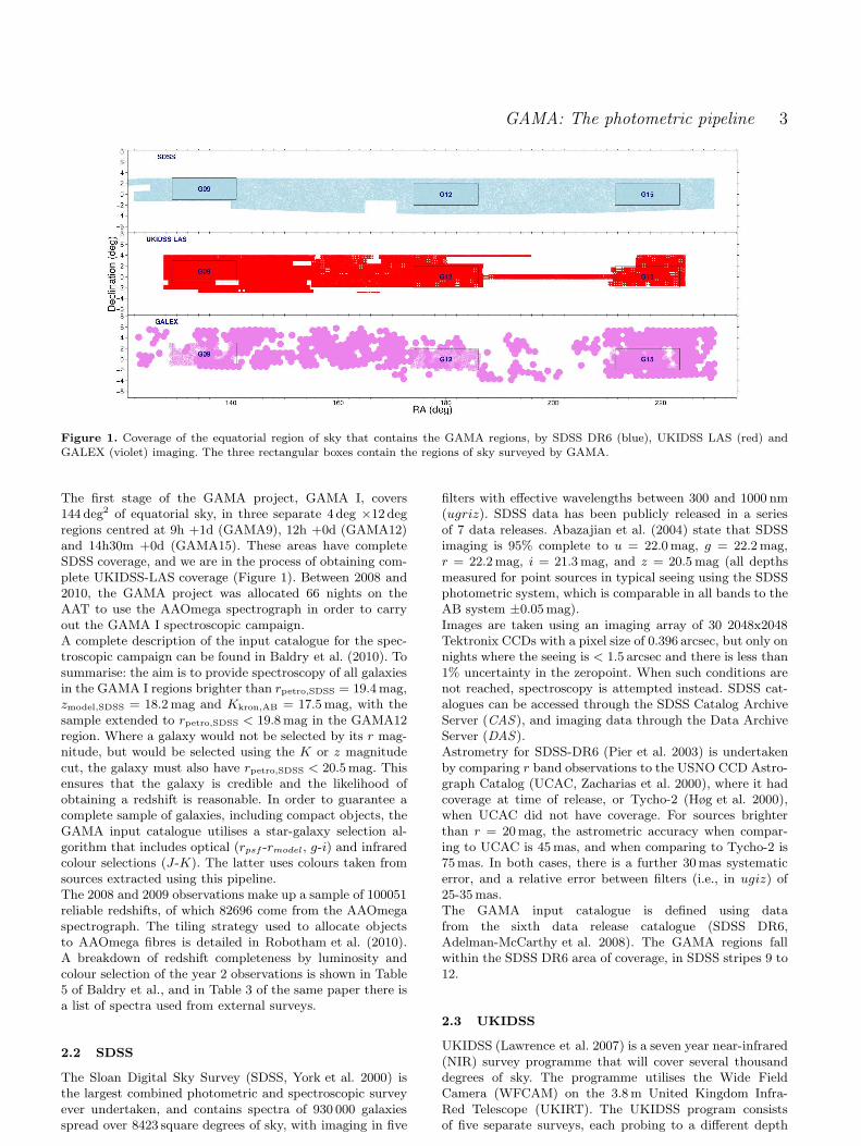
Figure 1. Coverage of the equatorial region of sky that contains the GAMA regions, by SDSS DR6 (blue), UKIDSS LAS (red) andGALEX (violet) imaging. The three rectangular boxes contain the regions of sky surveyed by GAMA.

The first stage of the GAMA project, GAMA I, covers144 deg2 of equatorial sky, in three separate 4 deg ×12 degregions centred at 9h +1d (GAMA9), 12h +0d (GAMA12)and 14h30m +0d (GAMA15). These areas have completeSDSS coverage, and we are in the process of obtaining com-plete UKIDSS-LAS coverage (Figure 1). Between 2008 and2010, the GAMA project was allocated 66 nights on theAAT to use the AAOmega spectrograph in order to carryout the GAMA I spectroscopic campaign.A complete description of the input catalogue for the spec-troscopic campaign can be found in Baldry et al. (2010). Tosummarise: the aim is to provide spectroscopy of all galaxiesin the GAMA I regions brighter than rpetro,SDSS = 19.4mag,zmodel,SDSS = 18.2mag and Kkron,AB = 17.5mag, with thesample extended to rpetro,SDSS < 19.8mag in the GAMA12region. Where a galaxy would not be selected by its r mag-nitude, but would be selected using the K or z magnitudecut, the galaxy must also have rpetro,SDSS < 20.5mag. Thisensures that the galaxy is credible and the likelihood ofobtaining a redshift is reasonable. In order to guarantee acomplete sample of galaxies, including compact objects, theGAMA input catalogue utilises a star-galaxy selection al-gorithm that includes optical (rpsf -rmodel, g-i) and infraredcolour selections (J-K). The latter uses colours taken fromsources extracted using this pipeline.The 2008 and 2009 observations make up a sample of 100051reliable redshifts, of which 82696 come from the AAOmegaspectrograph. The tiling strategy used to allocate objectsto AAOmega fibres is detailed in Robotham et al. (2010).A breakdown of redshift completeness by luminosity andcolour selection of the year 2 observations is shown in Table5 of Baldry et al., and in Table 3 of the same paper there isa list of spectra used from external surveys.

2.2 SDSS

The Sloan Digital Sky Survey (SDSS, York et al. 2000) isthe largest combined photometric and spectroscopic surveyever undertaken, and contains spectra of 930 000 galaxiesspread over 8423 square degrees of sky, with imaging in five

filters with effective wavelengths between 300 and 1000 nm(ugriz). SDSS data has been publicly released in a seriesof 7 data releases. Abazajian et al. (2004) state that SDSSimaging is 95% complete to u = 22.0mag, g = 22.2mag,r = 22.2mag, i = 21.3mag, and z = 20.5mag (all depthsmeasured for point sources in typical seeing using the SDSSphotometric system, which is comparable in all bands to theAB system ±0.05mag).Images are taken using an imaging array of 30 2048x2048Tektronix CCDs with a pixel size of 0.396 arcsec, but only onnights where the seeing is < 1.5 arcsec and there is less than1% uncertainty in the zeropoint. When such conditions arenot reached, spectroscopy is attempted instead. SDSS cat-alogues can be accessed through the SDSS Catalog ArchiveServer (CAS), and imaging data through the Data ArchiveServer (DAS).Astrometry for SDSS-DR6 (Pier et al. 2003) is undertakenby comparing r band observations to the USNO CCD Astro-graph Catalog (UCAC, Zacharias et al. 2000), where it hadcoverage at time of release, or Tycho-2 (Høg et al. 2000),when UCAC did not have coverage. For sources brighterthan r = 20mag, the astrometric accuracy when compar-ing to UCAC is 45mas, and when comparing to Tycho-2 is75mas. In both cases, there is a further 30mas systematicerror, and a relative error between filters (i.e., in ugiz) of25-35mas.The GAMA input catalogue is defined using datafrom the sixth data release catalogue (SDSS DR6,Adelman-McCarthy et al. 2008). The GAMA regions fallwithin the SDSS DR6 area of coverage, in SDSS stripes 9 to12.

2.3 UKIDSS

UKIDSS (Lawrence et al. 2007) is a seven year near-infrared(NIR) survey programme that will cover several thousanddegrees of sky. The programme utilises the Wide FieldCamera (WFCAM) on the 3.8m United Kingdom Infra-Red Telescope (UKIRT). The UKIDSS program consistsof five separate surveys, each probing to a different depth

4 Hill et al.

and for a different scientific purpose. One of these surveys,the UKIDSS Large Area Survey (LAS) will cover 4000 deg2

and will overlap with the SDSS stripes 9 to 16, 26 to 33and part of stripe 82. As the GAMA survey regions arewithin SDSS stripes 9 to 12, the LAS survey will providehigh density near-IR photometric coverage over the entireGAMA area. The UKIDSS-LAS survey observes to a fargreater depth (KLAS = 18.2mag using the Vega magni-tude system) than the previous Two-Micron All-Sky Survey(2MASS, K2MASS = 15.50mag using the Vega magnitudesystem).When complete, the LAS has target depths ofK = 18.2mag,H = 18.6mag, J = 19.9mag (after two passes; this paperuses only the first J pass which is complete to 19.5mag)and Y = 20.3mag (all depths measured use the Vega sys-tem for a point source with 5σ detection within a 2 arcsecaperture). Currently, observations have been conducted inthe equatorial regions, and will soon cover large swathes ofthe Northern Sky. It is designed to have a seeing FWHM of< 1.2 arcsec, photometric rms uncertainty of < ±0.02magand astrometric rms of < ±0.1 arcsec. Each position on thesky will be viewed for 40s per pass. All survey data for thispaper is taken from the fourth data release (DR4).The WFCAM Science Archive (WSA, Hambly et al. 2008)is the storage facility for post-pipeline, calibrated UKIDSSdata. It provides users with access to fits images and CASU-generated object catalogues for all five UKIDSS surveys. Wedo not use the CASU generated catalogues for a few rea-sons. Firstly, the CASU catalogues for early UKIDSS datareleases suffer from a fault where deblended objects are sig-nificantly brighter than their parent object, in some cases byseveral magnitudes (Smith et al. 2009; Hill et al. 2010). Sec-ondly, the CASU catalogues only contain circular aperturefluxes. Thirdly, CASU decisions (e.g., deblending and aper-ture sizes) are not consistent between filters. For instance,the aperture radius and centre used to calculate kpetro-

mag of a source is not necessarily the same as the apertureradius and centre used to calculate ypetromag or hpetro-mag. We require accurate extended-aperture colours; theCASU catalogues do not provide this.

3 CONSTRUCTION OF THE MOSAICS FROM

SDSS AND UKIDSS IMAGING

One of GAMA’s priorities is the accurate measurementof SEDs from as broad a wavelength range as possible.This is non-trivial when combining data from multiple sur-veys. While each survey may be internally consistent withdata collected contemporaneously, conditions between sur-veys can vary. In particular, seeing and zeropoint parametersmay greatly differ between frames. When matching betweensurveys one may find an object in the centre of the framein one survey is split across two frames in another survey.There may also be variation in the angular scale of a pixelbetween different instruments, and even when two instru-ments have the same pixel size, a shift of half of a pixelbetween two frames can cause significant difficulties in calcu-lating colours for small, low surface brightness objects. Fur-thermore, in order to use SExtractor in dual frame mode,the source-detection and the observation frame pixels mustbe calibrated to the same world coordinate system. In the

Zeropoint (AB mag) − u

Fre

quen

cy

26.0 27.0 28.0 29.0

01000200030004000500060007000

Zeropoint (AB mag) − g

Fre

quen

cy

26.0 27.0 28.0 29.0

01000200030004000500060007000

Zeropoint (AB mag) − rF

requ

ency

26.0 27.0 28.0 29.0

01000200030004000500060007000

Zeropoint (AB mag) − i

Fre

quen

cy

26.0 27.0 28.0 29.0

01000200030004000500060007000

Zeropoint (AB mag) − z

Fre

quen

cy

26.0 27.0 28.0 29.0

01000200030004000500060007000

Zeropoint (AB mag) − Y

Fre

quen

cy

26.0 27.0 28.0 29.00

500100015002000250030003500

Zeropoint (AB mag) − J

Fre

quen

cy

26.0 27.0 28.0 29.00

500100015002000250030003500

Zeropoint (AB mag) − H

Fre

quen

cy

26.0 27.0 28.0 29.00

500100015002000250030003500

Zeropoint (AB mag) − K

Fre

quen

cy

26.0 27.0 28.0 29.00

500100015002000250030003500

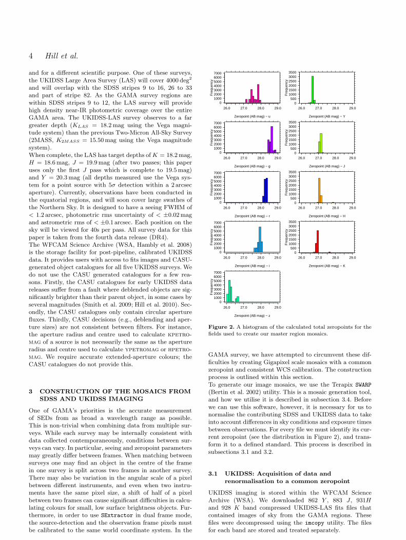
Figure 2. A histogram of the calculated total zeropoints for thefields used to create our master region mosaics.

GAMA survey, we have attempted to circumvent these dif-ficulties by creating Gigapixel scale mosaics with a commonzeropoint and consistent WCS calibration. The constructionprocess is outlined within this section.To generate our image mosaics, we use the Terapix SWARP

(Bertin et al. 2002) utility. This is a mosaic generation tool,and how we utilise it is described in subsection 3.4. Beforewe can use this software, however, it is necessary for us tonormalise the contributing SDSS and UKIDSS data to takeinto account differences in sky conditions and exposure timesbetween observations. For every file we must identify its cur-rent zeropoint (see the distribution in Figure 2), and trans-form it to a defined standard. This process is described insubsections 3.1 and 3.2.

3.1 UKIDSS: Acquisition of data and

renormalisation to a common zeropoint

UKIDSS imaging is stored within the WFCAM ScienceArchive (WSA). We downloaded 862 Y , 883 J , 931Hand 928 K band compressed UKIDSS-LAS fits files thatcontained images of sky from the GAMA regions. Thesefiles were decompressed using the imcopy utility. The filesfor each band are stored and treated separately.

GAMA: The photometric pipeline 5

Band AB offset (mag)

u -0.04g 0r 0i 0z +0.02Y 0.634J 0.938H 1.379K 1.900

Table 1. Conversion to AB magnitudes. The SDSS photometricsystem is roughly equivalent to the AB magnitude system, withonly small offsets in the u and z passbands. UKIDSS photometryis calculated on the Vega magnitude system, and our conversionsare from Hewett et al. (2006). Whilst we convert UKIDSS datausing a high precision parameter, it should be noted that the con-version uncertainty is only known to ∼ ±0.02mag (Cohen et al.2003).

A specially designed pipeline accesses each file, readsthe MAGZPT (ZPmag), EXP TIME (t), airmass(0.5 ∗ (AMSTART + AMEND) = secχmean) andEXTINCT (Ext) keywords from the fits header and createsa total AB magnitude zeropoint for the file using Equation 1.

ZPtotal = ZPmag−2.5log(1

t)−Ext× (secχmean−1)+ABVX

(1)where ABVX is the AB magnitude of Vega in the X band(Table 1).To correct each frame to a standard zeropoint (30), thevalue of each pixel is multiplied by a factor, calculatedusing Equation 2. Whilst we show the distribution of framezeropoints in Figure 2 in bins of 0.1mag, we use the actualzeropoint of each frame to calculate the total AB magnitudezeropoint. This has a far smaller variation (e.g., 0.02magin photometric conditions in the JHK filters; Warren et al.2007).

pixelmodifier = 10−0.4(ZPtotal−30) (2)

A new file is created to store the corrected pixel table,and the MAGZPT fits header parameter is updated. TheSKYLEVEL and SKYNOISE parameters are then scaledusing the same multiplying factor. This process takes 3 sec-onds per file.

3.2 SDSS: Acquisition of data and

renormalisation to a common zeropoint

The tsField and fpC files for the 12757 SDSS fields that coverthe GAMA regions were downloaded from the SDSS dataarchive server (das.sdss.org) for all five passbands. Again,the files for each passband are stored and treated separately.

We use a specially designed pipeline that brings in theaa (zeropoint), kk (extinction coefficient) and airmass key-words from a field’s tsField file, and the EXPTIME (t) key-word from the same field’s fpC file. Combining these usingEquation 3 we calculate the current total AB magnitude

Seeing (arcsec) − u

Fre

quen

cy

0.0 0.5 1.0 1.5 2.0 2.5 3.0

0500

100015002000250030003500

Seeing (arcsec) − g

Fre

quen

cy

0.0 0.5 1.0 1.5 2.0 2.5 3.0

0500

100015002000250030003500

Seeing (arcsec) − rF

requ

ency

0.0 0.5 1.0 1.5 2.0 2.5 3.0

0500

100015002000250030003500

Seeing (arcsec) − i

Fre

quen

cy

0.0 0.5 1.0 1.5 2.0 2.5 3.0

0500

100015002000250030003500

Seeing (arcsec) − z

Fre

quen

cy

0.0 0.5 1.0 1.5 2.0 2.5 3.0

0500

100015002000250030003500

Seeing (arcsec) − Y

Fre

quen

cy

0.0 0.5 1.0 1.5 2.0 2.5 3.0

0200400600800

10001200

Seeing (arcsec) − J

Fre

quen

cy

0.0 0.5 1.0 1.5 2.0 2.5 3.0

0200400600800

10001200

Seeing (arcsec) − H

Fre

quen

cy

0.0 0.5 1.0 1.5 2.0 2.5 3.0

0200400600800

10001200

Seeing (arcsec) − K

Fre

quen

cy

0.0 0.5 1.0 1.5 2.0 2.5 3.0

0200400600800

10001200

Figure 3. A histogram of the calculated seeing of the fields usedto create our master region mosaics.

zeropoint of the field (ZPtotal).

ZPtotal = −aa− 2.5log(1/t)− kk× airmass + sAo (3)

where sAo is the offset between the SDSS magnitude sys-tem and the actual AB magnitude system (−0.04mag for u,0.02mag for z, otherwise 0). The SDSS photometric zero-point uncertainty is estimated to be no larger than 0.03magin any band (Ivezic et al. 2004). We calculate the multiplierrequired to transform every pixel in the field (again usingEquation 2) to a standard zeropoint (30). As every pixelmust be modified by the same factor, we utilise the fcarithprogram (part of the Ftools package), to multiply the en-tire image by pixelmodifier. fcarith can normalise an SDSSimage every 1.25 seconds.

3.3 Correction of seeing bias

As observations were taken in different conditions thereis an intrinsic seeing bias between different input images,and between different filters (Figure 3). This could causeinaccuracies in photometric colour measurements that useapertures defined in one filter to derive magnitudes in asecond filter. To rectify this problem, it is necessary forus to degrade the better quality images to a lower seeing.

6 Hill et al.

However, if we degrade all images to our lowest qualityseeing (3.12 arcsec), we should lose the ability to resolvethe smallest galaxies in our sample. Therefore, we electto degrade our normalised images to 2 arcsec seeing. Thefraction of images with seeing worse than 2 arcsec is 4.4%,2.7%, 2.5%, 2.1%, 1.7%, 0%, 0%, 1.3% and 0.9% in u, g, r,i, z, Y , J , H and K, respectively. Images with worse seeingthan 2 arcsec are included in our degraded seeing mosaics.We do not attempt to modify their seeing. Although eachsurvey uses a different method of calculating the seeingwithin their data (SDSS use a double gaussian to modeltheir PSF, UKIDSS use the average FWHM of the stellarsources within the image), we assume that the seeingprovided for every frame is correct.To achieve a final PSF FWHM of 2 arcsec (σfinal) weassume that the seeing within an image follows a perfectGaussian distribution, σinitial. Theoretically, a Gaussiandistribution can be generated from the convolution of twoGaussian distributions. The fgauss utility (also part ofthe ftools package) can be used to convolve an inputimage with a circular Gaussian with a definable standarddeviation (σreq), calculated using Equation 4.

σreq =√

σ2final − σ2

initial (4)

As each UKIDSS frame has a different seeing value, itis necessary to break each fits file into its four constituentimages. This is not necessary for SDSS images (which arestored in separate files). However, it is necessary to retrievethe SDSS image seeing from the image’s tsField file. TheSDSS image seeing is stored in the psf width column of thetsField file. Where an image has a seeing better than ourspecified value, we use the fgauss utility to convolve ourimage down to our specified value. Where an image has aseeing worse than our specified value, we copy it withoutmodification using the imcopy utility. Both utilities producea set of UKIDSS files containing two HDUs: the originalinstrument header HDU and a single image HDUwith seeinggreater than or equal to our specified seeing. The outputSDSS files contain just a single image HDU. This processtakes approximated 2 seconds per frame.

3.4 Creation of master region images

The SWARP utility is a multi-thread capable co-addition andimage-warping tool that is part of the Terapix pipeline(Bertin et al. 2002). We use SWARP to generate complete im-ages of the GAMA regions from the normalised LAS/SDSSfits files. It is vital that the pixel size and area of coverage isthe same for each filter, as SExtractor’s dual-image moderequires perfectly matched frames. We define a pixel scaleof 0.4 × 0.4 arcsec, and generate 117000 × 45000 pixel filescentred around 09h00m00.0s, +01d00′00.0′′ (GAMA 9),12h00m00.0s, +00d00′00.0′′ (GAMA 12), and 14h30m00.0s,+00d00′00.0′′ (GAMA 15). SWARP is set to resample inputframes using the default LANCZOS3 algorithm, which theTerapix team found was the optimal option when workingwith images from the Megacam instrument (Bertin et al.2002).SWARP produces mosaics that use the TAN WCS projec-

tion system. As UKIDSS images are stored in the ZPNprojection system, SWARP internally converts the frames tothe TAN projection system. There is also an astrometricdistortion present in the UKIDSS images that SWARP

corrects using the pv2 3 and pv2 1 fits header parameters1.SWARP is set to subtract the background from the image, us-ing a background mesh of 256×256 pixels (102×102 arcsec)and a back filter size of 3 × 3 to calculate the back-ground map. The background calculation follows the samealgorithm as SExtractor (Bertin & Arnouts 1996). Tosummarise: it is a bicubic-spline interpolation between themeshes, with a median filter applied to remove bright starsand artifacts.Every mosaic contains pixels that are covered by multipleinput frames. SWARP is set to use the median pixel valuewhen a number of images overlap. The effects of outlyingpixel values, due to cosmic rays, bad pixels or CCD edges,should therefore be reduced. SWARP generates a weight map(Figure 4) that contains the flux variance in every pixel,calibrated using the background map described above.As the flux variance is affected by overlapping coverage,it is possible to see the survey footprint in the weightmap. The weight map can be used within SExtractor tocompensate for variations in noise. We do not use it whencalculating our photometry for two reasons. Firstly, there isoverlap between SDSS fpC frames. This overlap is not fromobservations, but from the method used to cut the longSDSS stripes into sections. SWARP would not account forthis, and the weighting of the overlap regions on the opticalmosaics would be calculated incorrectly. Secondly, usingthe weight maps would alter the effect of mosaic surfacebrightness limit variations upon our output catalogues. Aswe intend to model surface brightness effects later, we electto use an unweighted photometric catalogue.A small number of objects will be split between inputframes. SWARP can reconstruct them, with only small defectsdue to CCD edges. One such example is shown in Figure 5.We create both seeing-corrected and uncorrected mosaicsfor each passband and region combination. Each file is 20Gbin size. In total, the mosaics require just over 1 Terabyte ofstorage space. Each mosaic takes approximately 4 hours tocreate.

4 PHOTOMETRY

A major problem with constructing multi-wavelength cata-logues is that the definition of what constitutes an object canchange across the wavelength range (see Appendix A, par-ticularly Figure A1). This can be due to internal structuresuch as dust lanes or star forming regions becoming brighteror fainter in different passbands, causing the extraction soft-ware to deblend an object into a number of smaller parts inone filter but not in another. This can lead to large errors inthe resulting colours. We cannot be certain that the SDSSobject extraction process would produce the same results

1 An analysis of the astrometric distortion can be found in CASUdocument VDF-TRE-IOA-00009-0002 , currently available fromhttp://www.ast.cam.ac.uk/vdfs/docs/reports/astrom/index.html

GAMA: The photometric pipeline 7

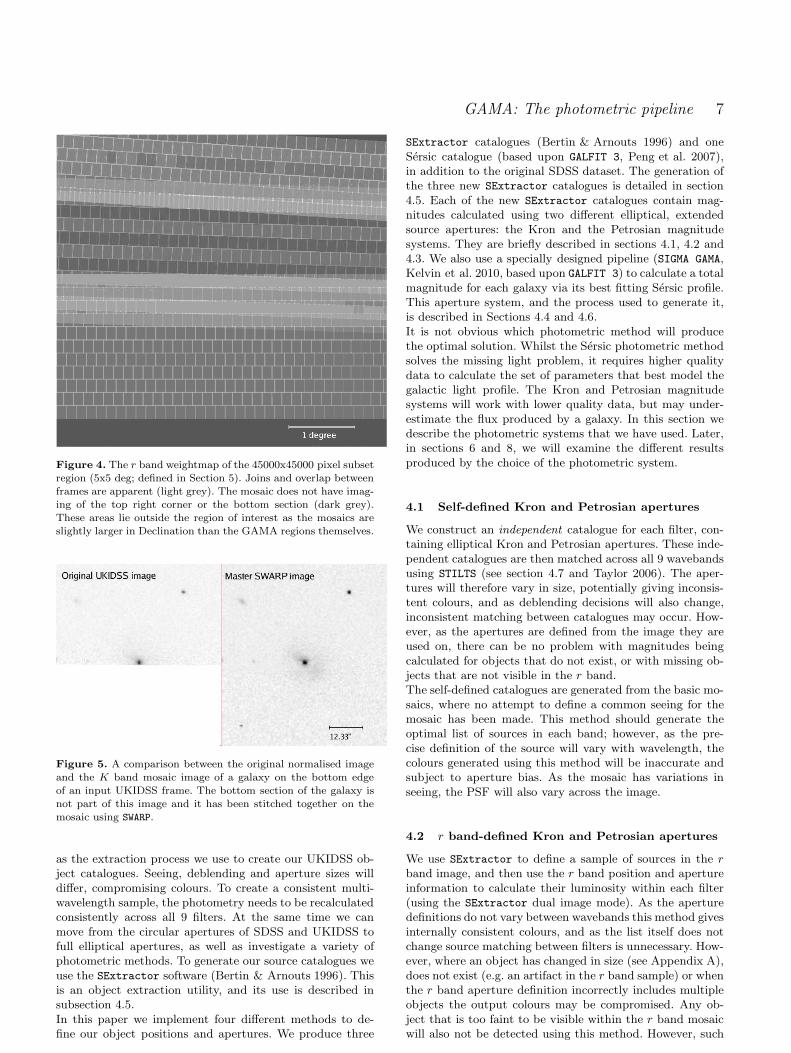
Figure 4. The r band weightmap of the 45000x45000 pixel subsetregion (5x5 deg; defined in Section 5). Joins and overlap betweenframes are apparent (light grey). The mosaic does not have imag-ing of the top right corner or the bottom section (dark grey).These areas lie outside the region of interest as the mosaics areslightly larger in Declination than the GAMA regions themselves.

Figure 5. A comparison between the original normalised imageand the K band mosaic image of a galaxy on the bottom edgeof an input UKIDSS frame. The bottom section of the galaxy isnot part of this image and it has been stitched together on themosaic using SWARP.

as the extraction process we use to create our UKIDSS ob-ject catalogues. Seeing, deblending and aperture sizes willdiffer, compromising colours. To create a consistent multi-wavelength sample, the photometry needs to be recalculatedconsistently across all 9 filters. At the same time we canmove from the circular apertures of SDSS and UKIDSS tofull elliptical apertures, as well as investigate a variety ofphotometric methods. To generate our source catalogues weuse the SExtractor software (Bertin & Arnouts 1996). Thisis an object extraction utility, and its use is described insubsection 4.5.In this paper we implement four different methods to de-fine our object positions and apertures. We produce three

SExtractor catalogues (Bertin & Arnouts 1996) and oneSersic catalogue (based upon GALFIT 3, Peng et al. 2007),in addition to the original SDSS dataset. The generation ofthe three new SExtractor catalogues is detailed in section4.5. Each of the new SExtractor catalogues contain mag-nitudes calculated using two different elliptical, extendedsource apertures: the Kron and the Petrosian magnitudesystems. They are briefly described in sections 4.1, 4.2 and4.3. We also use a specially designed pipeline (SIGMA GAMA,Kelvin et al. 2010, based upon GALFIT 3) to calculate a totalmagnitude for each galaxy via its best fitting Sersic profile.This aperture system, and the process used to generate it,is described in Sections 4.4 and 4.6.It is not obvious which photometric method will producethe optimal solution. Whilst the Sersic photometric methodsolves the missing light problem, it requires higher qualitydata to calculate the set of parameters that best model thegalactic light profile. The Kron and Petrosian magnitudesystems will work with lower quality data, but may under-estimate the flux produced by a galaxy. In this section wedescribe the photometric systems that we have used. Later,in sections 6 and 8, we will examine the different resultsproduced by the choice of the photometric system.

4.1 Self-defined Kron and Petrosian apertures

We construct an independent catalogue for each filter, con-taining elliptical Kron and Petrosian apertures. These inde-pendent catalogues are then matched across all 9 wavebandsusing STILTS (see section 4.7 and Taylor 2006). The aper-tures will therefore vary in size, potentially giving inconsis-tent colours, and as deblending decisions will also change,inconsistent matching between catalogues may occur. How-ever, as the apertures are defined from the image they areused on, there can be no problem with magnitudes beingcalculated for objects that do not exist, or with missing ob-jects that are not visible in the r band.The self-defined catalogues are generated from the basic mo-saics, where no attempt to define a common seeing for themosaic has been made. This method should generate theoptimal list of sources in each band; however, as the pre-cise definition of the source will vary with wavelength, thecolours generated using this method will be inaccurate andsubject to aperture bias. As the mosaic has variations inseeing, the PSF will also vary across the image.

4.2 r band-defined Kron and Petrosian apertures

We use SExtractor to define a sample of sources in the rband image, and then use the r band position and apertureinformation to calculate their luminosity within each filter(using the SExtractor dual image mode). As the aperturedefinitions do not vary between wavebands this method givesinternally consistent colours, and as the list itself does notchange source matching between filters is unnecessary. How-ever, where an object has changed in size (see Appendix A),does not exist (e.g. an artifact in the r band sample) or whenthe r band aperture definition incorrectly includes multipleobjects the output colours may be compromised. Any ob-ject that is too faint to be visible within the r band mosaicwill also not be detected using this method. However, such

8 Hill et al.

objects will be fainter than the GAMA sample’s selectioncriteria, and would not be included within our sample. Ther band-defined catalogues are generated from our seeing-degraded mosaics. They provide us with an optically-definedsource sample.This method is analogous to the SDSS source catalogues,which define their apertures using the r passband data (un-less the object is not detected in r, in which case a dif-ferent filter is chosen). However, the GAMA photometricpipeline has a broader wavelength range as it now includesNIR measurements from the same aperture definition. Fur-thermore, the SDSS Petrosian magnitudes have not beenseeing-standardised. While all data is taken at the sametime, the diffraction limit is wavelength dependent and dif-ferent fractions of light will be missed despite the use of afixed aperture. SDSS model magnitudes do account for theeffects of the PSF.

4.3 K band-defined Kron and Petrosian apertures

This method works in the same way as the previous method,but uses the K band image as the detection frame ratherthan the r band image. We are limited in the total area,as the K band coverage is currently incomplete. However,for samples that require complete colour coverage in all 9filters, this is not a problem. As with r band-defined cata-logues, the K band-defined catalogues are generated fromthe seeing-corrected mosaics. They provide us with a NIR-defined source sample. The K-band defined Kron magni-tudes were used in the GAMA input catalogue (Baldry et al.2010) to calculate the star-galaxy separation J − K colourand the K band target selection.

4.4 Sersic magnitudes

We use the SIGMA modelling wrapper (see section 4.6 andKelvin et al. 2010 for more details) which in turn uses thegalaxy fitting software GALFIT 3.0 (Peng et al. 2007) to fita single-Sersic component to each object independently in9 filters (ugrizY JHK), and recover their Sersic magni-tudes, indices, effective radii, position angles and elliptici-ties. Source positions are initially taken from the GAMA in-put catalogue, as defined in Baldry et al. (2010). All Sersicmagnitudes are self-defined; as each band is modelled inde-pendently of the others, the aperture definition will vary andcolour may therefore be compromised.Single-Sersic fitting is comparable to the SDSS model mag-nitudes. SIGMA therefore should recover total fluxes for ob-jects that have a Sersic index in the range 0.3 < n < 20,where model magnitudes force a fit to either an exponen-tial (n=1) or deVaucouleurs (n=4) profile. The systematicmagnitude errors that arise when model magnitudes are fitto galaxies that do not follow an exponential or deVau-couleurs profile (Graham 2001; Brown et al. 2003) do notoccur in SIGMA. The SDSS team developed a composite mag-nitude system, cmodel, that calculates a magnitude fromthe combination of the n=1 and n=4 systems, in order to cir-cumvent this issue (Abazajian et al. 2004). We compare ourSersic magnitudes to their results later. Sersic magnitudes donot suffer from the missing-flux issue that affects Kron andPetrosian apertures. Petrosian magnitudes may underesti-mate a galaxy’s luminosity by 0.2mag (Strauss et al. 2002),

while under certain conditions a Kron aperture may only re-cover half of a galaxy’s total luminosity (Andreon 2002). TheSersic catalogues are generated from the seeing-uncorrectedmosaics, as the seeing parameters are modelled within SIGMA

using the PSFEx software utility (E. Bertin, priv. comm).

4.5 Object Extraction of Kron and Petrosian

apertures

The SExtractor utility (Bertin & Arnouts 1996) is a pro-gram that generates catalogues of source positions and aper-ture fluxes from an input image. It has the capacity todefine the sources and apertures in one frame and calcu-late the corresponding fluxes in a second frame. This dualimage mode is computationally more intensive than thestandard SExtractor single image mode (in single imagemode, SExtractor can extract a catalogue from a mosaicwithin a few hours; dual image mode takes a few daysper mosaic). Using the u, g, r, i, z, Y , J , H and K im-ages created by the SWARP utility, we define our catalogueof sources independently (for the self-defined catalogues),using the r band mosaics (for the r band-defined cata-logue) or the K band mosaics (for the K band-defined cat-alogue) and calculate their flux in all nine bands. The nor-malisation and SWARP processes removed the image back-ground and standardised the zeropoint; we therefore usea constant MAG ZEROPOINT=30, and BACK VALUE=0.SExtractor generates both elliptical Petrosian (2.0 RPetro)and Kron-like apertures (2.5 RKron, called AUTO magni-tudes). SExtractor Petrosian magnitudes are computed us-ing 1

νRPetro= 0.2, the same parameter as SDSS. As the

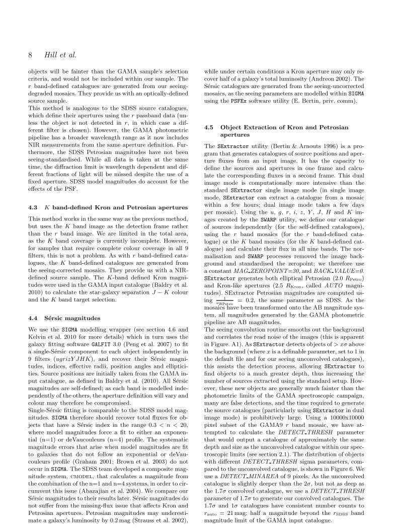
mosaics have been transformed onto the AB magnitude sys-tem, all magnitudes generated by the GAMA photometricpipeline are AB magnitudes.The seeing convolution routine smooths out the backgroundand correlates the read noise of the images (this is apparentin Figure. A1). As SExtractor detects objects of > xσ abovethe background (where x is a definable parameter, set to 1 inthe default file and for our seeing unconvolved catalogues),this assists the detection process, allowing SExtractor tofind objects to a much greater depth, thus increasing thenumber of sources extracted using the standard setup. How-ever, these new objects are generally much fainter than thephotometric limits of the GAMA spectroscopic campaign,many are false detections, and the time required to generatethe source catalogues (particularly using SExtractor in dualimage mode) is prohibitively large. Using a 10000x10000pixel subset of the GAMA9 r band mosaic, we have at-tempted to calculate the DETECT THRESH parameterthat would output a catalogue of approximately the samedepth and size as the unconvolved catalogue within our spec-troscopic limits (see section 2.1). The distribution of objectswith different DETECT THRESH sigma parameters, com-pared to the unconvolved catalogue, is shown in Figure 6. Weuse a DETECT MINAREA of 9 pixels. As the unconvolvedcatalogue is slightly deeper than the 2σ, but not as deep asthe 1.7σ convolved catalogue, we use a DETECT THRESH

parameter of 1.7σ to generate our convolved catalogues. The1.7σ and 1σ catalogues have consistent number counts torauto = 21mag; half a magnitude beyond the rSDSS bandmagnitude limit of the GAMA input catalogue.

GAMA: The photometric pipeline 9

rAUTO(mag)

N(m

) dm

50

100

500

10001000

5000

18 19 20 21 22 23 24 25

Detection threshold

1 sigma

1.2 sigma

1.5 sigma

1.7 sigma

Unconvolved 1 sigma

2 sigma

2.5 sigma

3 sigma

5 sigma

Figure 6. The effects of changing the SExtractor DE-TECT THRESH parameter on a subset of an r band mosaic.The dotted black line is the deepest r band sample limit of theGAMA survey (for those objects that are K or z selected).

4.6 Object extraction for Sersic magnitudes

Sersic magnitudes are obtained as an output from thegalaxy modelling program SIGMA (Structural Investigationof Galaxies via Model Analysis) written in the R program-ming language (Kelvin et al. 2010). In brief, SIGMA takesthe Right Ascension and Declination of an object that haspassed our star-galaxy separation criteria and calculates itspixel position within the appropriate mosaic. A square re-gion, centred on the object, is cut out from the mosaic con-taining a minimum of 20 guide stars with which to generatea PSF. SExtractor then provides a FITS-standard inputcatalogue to PSF Extractor (E. Bertin, priv. comm.) whichgenerates an empirical PSF for each image. Ellipticities andposition angles are obtained from the STSDAS Ellipse

routine within IRAF, and provides an input to Galfit. Thelarger cutout is again cut down to a region which contains90% of the target object’s flux plus a buffer of 10 pixels,and will only deviate from this size if a bright nearby objectcauses the fitting region to be expanded in order to modelany satellites the target may have.GALFIT 3 is then used to fit a single-Sersic component toeach target, and several runs may be attempted if, for exam-ple, the previous run crashed, the code reached its maximumnumber of iterations, the centre has migrated to fit a sep-arate object, the effective radius is too high or low or theSersic index is too large. SIGMA employs a complex eventhandler in order to run the code as many times as neces-sary to fix these problems, however not all problems can befixed, and so residual quality flags remain to reflect the qual-ity of the final fit. The SIGMA package takes approximately10 seconds per object. For full details of the SIGMA modellingprogram, see Kelvin et al. (2010).

4.7 Catalogue matching

The definition of the GAMA spectroscopic target selection(herein referred to as the tiling catalogue) is detailed inBaldry et al. (2010), and is based on original SDSS DR6data. We therefore need to relate our revised photometryback to this catalogue in order to connect it to our AAOmegaspectra. The tiling catalogue utilises a mask around brightstars that should remove most objects with bad photometryand erroneously bright magnitudes, as well as implement-ing a revised star-galaxy separation quantified against ourspectroscopic results. It has been extensively tested, withsources that are likely to be artifacts, bad deblends or sec-tions of larger galaxies viewed a number of times by differentpeople. By matching our catalogues to the tiling catalogue,we can access the results of this rigorous filtering process,and generate a full, self-consistent set of colours for all of theobjects that are within the GAMA sample (and are withinregions that have been observed in all nine passbands). Asthe tiling catalogue is also used when redshift targeting, wewill be able to calculate the completeness in all the pass-bands of the GAMA survey. The GAMA tiling catalogue isa subset of the GAMA master catalogue (herein referred toas the master catalogue). The master catalogue is createdusing the SDSS DR6 catalogue stored on the CAS2. Un-like the master catalogue, the tiling catalogue undertakesstar-galaxy separation, and applies surface brightness andmagnitude selection.STILTS (Taylor 2006) is a catalogue combination tool, witha number of different modes. We use it to join our regioncatalogues together to create r-defined, K-defined and self-defined aperture photometry catalogues that cover the entireGAMA area. We also use it to match these catalogues to theGAMA tiling catalogue.

4.8 Source catalogues

The catalogues that have been generated are listed inTable 2. The syntax of the Key column is as follows.X[u] means a u band magnitude from an X band-definedaperture, u means a self-defined u band magnitudeand + denotes a STILTS tskymatch2 5 arcsec, uniquenearest-object match between two catalogues (see Section4.7). Where two datasets are combined together withoutthe + notation (i.e., the final two lines), this denotesa STILTS tmatch2, matcher=“exact“ match using SDSSobjid as the primary key. Note that in a set of self-definedsamples (ugrizY JHK), each sample must be matchedseparately (as each contains a different set of sources),and then combined. This is not the case in the aperturedefined samples (where each sample contains the same setof sources). Subscripts denote the photometric method used

2 We use the query SELECT * FROM dr6.PhotoObj as pWHERE ( p.modelmag r - p.extinction r < 20.5 or p.petromag r- p.extinction r < 19.8 ) and ( (p.ra > 129.0 and p.ra < 141.0 andp.dec > -1.0 and p.dec < 3.0) or (p.ra > 174.0 and p.ra < 186.0and p.dec > -2.0 and p.dec < 2.0) or (p.ra > 211.5 and p.ra <

223.5 and p.dec > -2.0 and p.dec < 2.0) ) and ((p.mode = 1) or(p.mode = 2 and p.ra < 139.939 and p.dec < -0.5 and (p.status& dbo.fphotostatus(’OK SCANLINE’)) > 0))

10 Hill et al.

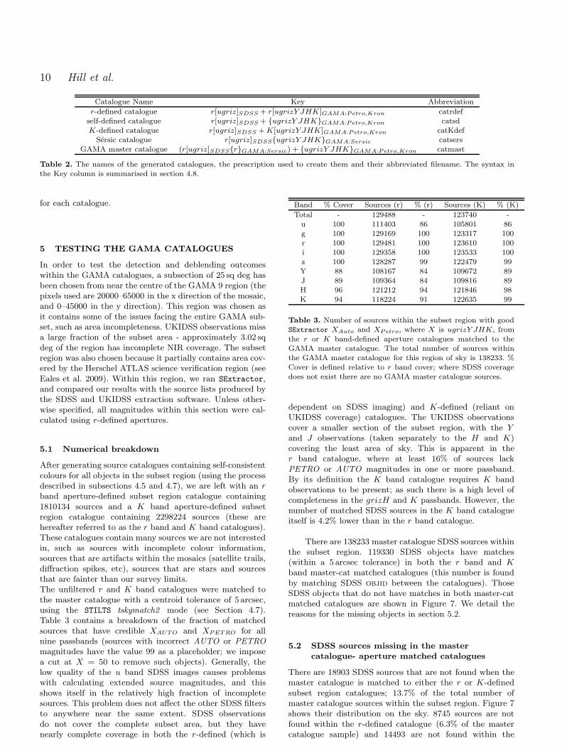
Catalogue Name Key Abbreviation

r-defined catalogue r[ugriz]SDSS + r[ugrizY JHK]GAMA:Petro,Kron catrdefself-defined catalogue r[ugriz]SDSS + ugrizY JHKGAMA:Petro,Kron catsdK-defined catalogue r[ugriz]SDSS +K[ugrizY JHK]GAMA:Petro,Kron catKdefSersic catalogue r[ugriz]SDSSugrizY JHKGAMA:Sersic catsers

GAMA master catalogue (r[ugriz]SDSSrGAMA:Sersic) + ugrizY JHKGAMA:Petro,Kron catmast

Table 2. The names of the generated catalogues, the prescription used to create them and their abbreviated filename. The syntax inthe Key column is summarised in section 4.8.

for each catalogue.

5 TESTING THE GAMA CATALOGUES

In order to test the detection and deblending outcomeswithin the GAMA catalogues, a subsection of 25 sq deg hasbeen chosen from near the centre of the GAMA 9 region (thepixels used are 20000–65000 in the x direction of the mosaic,and 0–45000 in the y direction). This region was chosen asit contains some of the issues facing the entire GAMA sub-set, such as area incompleteness. UKIDSS observations missa large fraction of the subset area - approximately 3.02 sqdeg of the region has incomplete NIR coverage. The subsetregion was also chosen because it partially contains area cov-ered by the Herschel ATLAS science verification region (seeEales et al. 2009). Within this region, we ran SExtractor,and compared our results with the source lists produced bythe SDSS and UKIDSS extraction software. Unless other-wise specified, all magnitudes within this section were cal-culated using r-defined apertures.

5.1 Numerical breakdown

After generating source catalogues containing self-consistentcolours for all objects in the subset region (using the processdescribed in subsections 4.5 and 4.7), we are left with an rband aperture-defined subset region catalogue containing1810134 sources and a K band aperture-defined subsetregion catalogue containing 2298224 sources (these arehereafter referred to as the r band and K band catalogues).These catalogues contain many sources we are not interestedin, such as sources with incomplete colour information,sources that are artifacts within the mosaics (satellite trails,diffraction spikes, etc), sources that are stars and sourcesthat are fainter than our survey limits.The unfiltered r and K band catalogues were matched tothe master catalogue with a centroid tolerance of 5 arcsec,using the STILTS tskymatch2 mode (see Section 4.7).Table 3 contains a breakdown of the fraction of matchedsources that have credible XAUTO and XPETRO for allnine passbands (sources with incorrect AUTO or PETRO

magnitudes have the value 99 as a placeholder; we imposea cut at X = 50 to remove such objects). Generally, thelow quality of the u band SDSS images causes problemswith calculating extended source magnitudes, and thisshows itself in the relatively high fraction of incompletesources. This problem does not affect the other SDSS filtersto anywhere near the same extent. SDSS observationsdo not cover the complete subset area, but they havenearly complete coverage in both the r-defined (which is

Band % Cover Sources (r) % (r) Sources (K) % (K)

Total - 129488 - 123740 -u 100 111403 86 105801 86g 100 129169 100 123317 100r 100 129481 100 123610 100i 100 129358 100 123533 100z 100 128287 99 122479 99Y 88 108167 84 109672 89J 89 109364 84 109816 89H 96 121212 94 121846 98K 94 118224 91 122635 99

Table 3. Number of sources within the subset region with goodSExtractor XAuto and XPetro, where X is ugrizY JHK, fromthe r or K band-defined aperture catalogues matched to theGAMA master catalogue. The total number of sources withinthe GAMA master catalogue for this region of sky is 138233. %Cover is defined relative to r band cover; where SDSS coveragedoes not exist there are no GAMA master catalogue sources.

dependent on SDSS imaging) and K-defined (reliant onUKIDSS coverage) catalogues. The UKIDSS observationscover a smaller section of the subset region, with the Yand J observations (taken separately to the H and K)covering the least area of sky. This is apparent in ther band catalogue, where at least 16% of sources lackPETRO or AUTO magnitudes in one or more passband.By its definition the K band catalogue requires K bandobservations to be present; as such there is a high level ofcompleteness in the grizH and K passbands. However, thenumber of matched SDSS sources in the K band catalogueitself is 4.2% lower than in the r band catalogue.

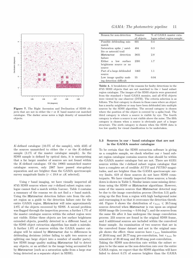
There are 138233 master catalogue SDSS sources withinthe subset region. 119330 SDSS objects have matches(within a 5 arcsec tolerance) in both the r band and Kband master-cat matched catalogues (this number is foundby matching SDSS objid between the catalogues). ThoseSDSS objects that do not have matches in both master-catmatched catalogues are shown in Figure 7. We detail thereasons for the missing objects in section 5.2.

5.2 SDSS sources missing in the master

catalogue- aperture matched catalogues

There are 18903 SDSS sources that are not found when themaster catalogue is matched to either the r or K-definedsubset region catalogues; 13.7% of the total number ofmaster catalogue sources within the subset region. Figure 7shows their distribution on the sky. 8745 sources are notfound within the r-defined catalogue (6.3% of the mastercatalogue sample) and 14493 are not found within the

GAMA: The photometric pipeline 11

135 136 137 138 139

−1

01

23

RA (degrees)

Dec

linat

ion

(deg

rees

)

Figure 7. The Right Ascension and Declination of SDSS ob-jects that are not in either the r or K band master-cat matchedcatalogue. The darker areas notes a high density of unmatchedobjects.

K-defined catalogue (10.5% of the sample), with 4335 ofthe sources unmatched to either the r or the K-definedsample (3.1% of the master catalogue sample). As theSDSS sample is defined by optical data, it is unsurprisingthat a far larger number of sources are not found withinthe K-defined catalogue. Of the 18903 unmatched mastercatalogue sources, only 2367 have passed star-galaxyseparation and are brighter than the GAMA spectroscopicsurvey magnitude limits (r < 19.8 or zK selected).

Using r band imaging, we have visually inspected all8745 SDSS sources where our r-defined subset region cata-logue cannot find a match within 5 arcsec. Table 4 containsa summary of the reasons we do not find a r band match.Using the SExtractor detection failure rate from the sub-set region as a guide to the detection failure rate for theentire GAMA region, SExtractor will miss approximately2.8% of the objects recovered by SDSS. A second problemwas flagged through the inspection process; a further 1.7% ofthe master catalogue sources within the subset region werenot visible. Either these objects are low surface brightnessextended objects, possibly detected in a different band, orthe SDSS object extraction algorithm has made a mistake.A further 1.8% of sources within the GAMA master cat-alogue will be missed by SExtractor due to differences indeblending decisions (either failing to split two sources orsplitting one large object into a number of smaller parts),low SDSS image quality making SExtractor fail to detectany objects, or an artifact in the image being accounted forby SExtractor (such as a saturation spike from a large starbeing detected as a separate object in SDSS).

Reason for non-detection Numberof objects

% of GAMA master cata-logue subset region sample

Possible deblending mis-match

601 0.4

Saturation spike / satel-lite or asteroid trail

404 0.3

SExtractor detectionfailure

3831 2.8

Either a low surfacebrightness source or nosource

2391 1.7

Part of a large deblendedsource

1463 1.1

Low image quality mak-ing detection difficult

55 0.04

Table 4. A breakdown of the reasons for faulty detections in the8745 SDSS objects that are not matched to the r band subsetregion catalogue. The images of the SDSS objects were generatedfrom the standard r band GAMA mosaics, and all 8745 objectswere viewed by one observer (DTH). The criteria selection is as

follows. The first category is chosen in those cases where an objecthas a nearby neighbour or may have been deblended into multiplesources by the SDSS algorithm. The second category is chosenwhere the position of the object is covered by a spike/trail. Thethird category is where a source is visible by eye. The fourthcategory is where a source is not visible above the noise. The fifthcategory is chosen when a source is obviously part of a largerstructure. The sixth category is chosen when the SDSS data istoo low quality for visual classification to be undertaken.

5.3 Sources in our r band catalogue that are not

in the GAMA master catalogue

To be certain that the SDSS extraction software is givingus a complete sample, we check whether our r band sub-set region catalogue contains sources that should be withinthe GAMA master catalogue but are not. There are 61351sources within the r-defined subset region catalogue thathave a complete set of credible AUTO and PETRO magni-tudes, and are brighter than the GAMA spectroscopic sur-vey limits. 619 of these sources do not have SDSS coun-terparts. We have visually inspected these sources; a break-down is shown in Table 5. Similar issues cause missing detec-tions using the SDSS or SExtractor algorithms. However,some of the unseen sources that SExtractor detected maybe due to the image convolution process (Section 3.3) gath-ering up the flux from a region with high background noiseand rearranging it so that it overcomes the detection thresh-old. Figure 8 shows the distribution of rAuto 6 20.5magsources detected when SExtractor is run upon an originalSDSS image file (covering ∼ 0.04 deg2), and the sources fromthe same file after it has undergone the image convolutionprocess. 233 sources are found in the original SDSS frame,and 3 additional sources are included within the convolvedframe sample. An examination of two sources that are inthe convolved frame dataset and not in the original sam-ple shows the effect: these sources have rAuto luminositiesof 20.64mag and 20.77mag pre-convolution, but rAuto lu-minosities of 20.40mag and 20.48mag post-convolution.Taking the SDSS non-detection rate within the subset re-gion to be the same as the non-detection rate over the entireGAMA region, we expect that the SDSS algorithm will havefailed to detect 0.1% of sources brighter than the GAMA

12 Hill et al.

Type of source Number of objects

Source 171No visible source 274

Section of bright star 163Possible deblend mismatch 10

Low image quality making detection difficult 1

Table 5. A breakdown of the 619 r-defined subset region cat-alogue objects brighter than the GAMA sample limits that arenot matched to the GAMA master catalogue.The images of thesubset region catalogue objects were generated from the standardr band GAMA mosaics, and all 619 objects were viewed by oneobserver (DTH).

Figure 8. A comparison between the objects detected whenSExtractor is run over an original SDSS image, and when it isrun over the convolved, mosaic imaging. Yellow circles are sourceswith r 6 20.5mag detected from the GAMA mosaic, red crossesare sources that are detected from the original SDSS data.

spectroscopic survey limits; approximately 1000 sources willnot have been included within the master catalogue.

5.4 Sources in our K band catalogue that are not

in the UKIDSS DR5PLUS database

We have also tested the UKIDSS DR5 catalogue. Wehave generated a catalogue from the WSA that selects allUKIDSS objects within the GAMA subset region3, and wehave matched this catalogue to the K band-defined subsetregion catalogue. From the 69537 K band-defined subsetregion catalogue sources, there are 4548 sources that havenot been matched to an UKIDSS object within a toleranceof 5 arcsec. We have visually inspected K band images ofthose objects that are brighter than the GAMA spectro-scopic survey K band limit (KAUTO 6 17.6mag). We findthat 29 of the 117 unmatched objects are real sources thatare missed by the UKIDSS extraction software; a negligi-ble fraction of the entire dataset. A large (but unquantified)fraction of the other 88 sources are suffering from the convo-lution flux-redistribution problem discussed in Section 5.3.The background fluctuations in K band data are greaterthan in the r band, making this a much greater problem.

3 We use the query ”SELECT las.ra, las.dec, las.kPetroMagFROM lasSource as las WHERE las.ra < 139.28 AND las.ra >

134.275 AND las.dec > −1 AND las.dec < 3”

6 PROPERTIES OF THE CATALOGUES

6.1 Constructing a clean sample

In order to investigate the photometric offsets betweendifferent photometric systems, we require a sample ofgalaxies with a complete set of credible photometry that areunaffected by deblending decisions. This has been createdvia the following prescription. We match the r-definedaperture catalogue to the GAMA master catalogue with atolerance of 5 arcsec. We remove any GAMA objects thathave not been matched, or have been matched to multipleobjects within that tolerance (when run in All match modeSTILTS produces a GroupSize column, where a NULL valuesignifies no group). We then match to the 9 self-definedobject catalogues, in each case removing all unmatchedand multiply matched GAMA objects. As our convolutionroutine will cause problems with those galaxies that containsaturated pixels, we also remove those galaxies that areflagged as saturated by SDSS. This sample is then linkedto the Sersic pipeline catalogue (using the SDSS objid asthe primary key). We remove all those Sersic magnitudeswhere the pipeline has flagged that the model is badlyfit or where the photometry has been compromised andmatch to the K band aperture-defined catalogue, againwith unmatched and multiple matched sources removed.This gives us a final population of 18065 galaxies thathave clean r-defined, K-defined, self-defined and Sersicmagnitudes, are not saturated and cannot have beenmismatched. Having constructed a clean, unambiguoussample of common objects, any photometric offset can onlybe due to differences between the photometric systemsused. As we remove objects that are badly fit by the Sersicpipeline, it should be noted that the resulting sample will,by its definition, only contain sources that have a lightprofile that can be fitted using the Sersic function.

6.2 Photometric offset between systems

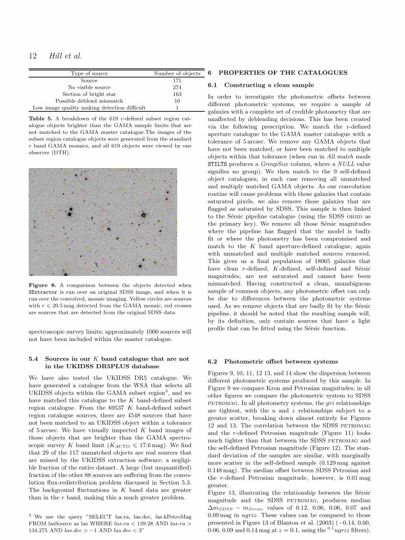
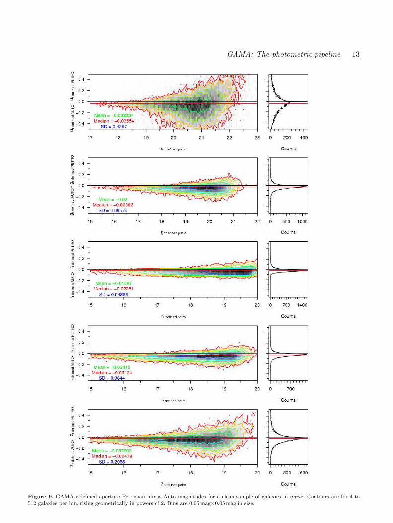
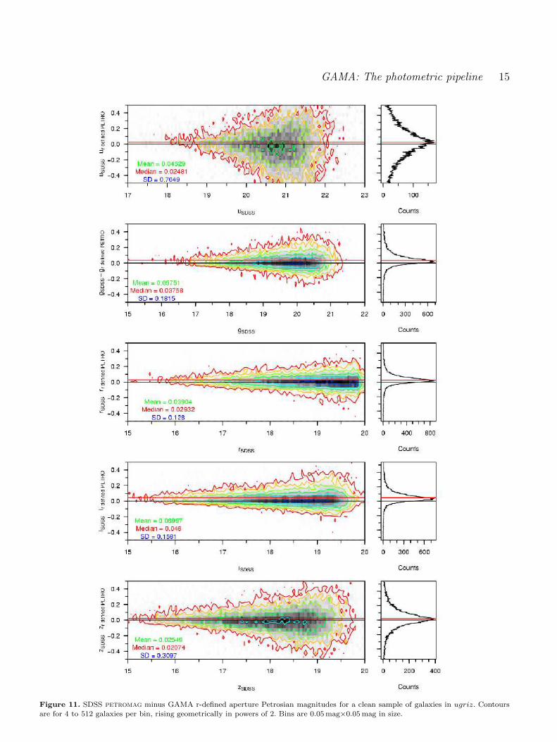
Figures 9, 10, 11, 12 13, and 14 show the dispersion betweendifferent photometric systems produced by this sample. InFigure 9 we compare Kron and Petrosian magnitudes; in allother figures we compare the photometric system to SDSSpetromag. In all photometry systems, the gri relationshipsare tightest, with the u and z relationships subject to agreater scatter, breaking down almost entirely for Figures12 and 13. The correlation between the SDSS petromag

and the r-defined Petrosian magnitude (Figure 11) looksmuch tighter than that between the SDSS petromag andthe self-defined Petrosian magnitude (Figure 12). The stan-dard deviation of the samples are similar, with marginallymore scatter in the self-defined sample (0.129mag against0.148mag). The median offset between SDSS Petrosian andthe r-defined Petrosian magnitude, however, is 0.01maggreater.Figure 13, illustrating the relationship between the Sersicmagnitude and the SDSS petromag, produces median∆mSDSS − mSersic values of 0.12, 0.06, 0.06, 0.07 and0.09mag in ugriz. These values can be compared to thosepresented in Figure 13 of Blanton et al. (2003) (−0.14, 0.00,0.06, 0.09 and 0.14mag at z = 0.1, using the 0.1ugriz filters),

GAMA: The photometric pipeline 13

Figure 9. GAMA r-defined aperture Petrosian minus Auto magnitudes for a clean sample of galaxies in ugriz. Contours are for 4 to512 galaxies per bin, rising geometrically in powers of 2. Bins are 0.05mag×0.05mag in size.

14 Hill et al.

Figure 10. SDSS petromag minus GAMA r-defined aperture Auto magnitudes for a clean sample of galaxies in ugriz. Contours arefor 4 to 512 galaxies per bin, rising geometrically in powers of 2. Bins are 0.05mag×0.05mag in size.

GAMA: The photometric pipeline 15

Figure 11. SDSS petromag minus GAMA r-defined aperture Petrosian magnitudes for a clean sample of galaxies in ugriz. Contoursare for 4 to 512 galaxies per bin, rising geometrically in powers of 2. Bins are 0.05mag×0.05mag in size.

16 Hill et al.

Figure 12. SDSS petromag minus GAMA self-defined aperture Petrosian magnitudes for a clean sample of galaxies in ugriz. Contoursare for 4 to 512 galaxies per bin, rising geometrically in powers of 2. Bins are 0.05mag×0.05mag in size.

GAMA: The photometric pipeline 17

Figure 13. SDSS petromag minus GAMA Sersic magnitudes for a clean sample of galaxies in ugriz. Contours are for 4 to 512 galaxiesper bin, rising geometrically in powers of 2. Bins are 0.05mag×0.05mag in size.

18 Hill et al.

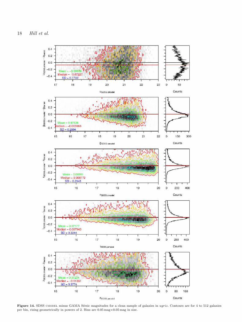
Figure 14. SDSS cmodel minus GAMA Sersic magnitudes for a clean sample of galaxies in ugriz. Contours are for 4 to 512 galaxiesper bin, rising geometrically in powers of 2. Bins are 0.05mag×0.05mag in size.

GAMA: The photometric pipeline 19

given the variance in the relationship (the standard devia-tion in our samples are 0.77, 0.28, 0.21, 0.22 and 0.40mag,respectively). A significant fraction (∼ 28%) of the sam-ple has rSDSS − rSersic¿0.5mag, and therefore lies beyondthe boundaries of this image. These offsets are significant,and will be discussed further in Section 7. We can say thatthe r-defined aperture photometry is the closest match toSDSS petromag photometry. Figure 14 shows the relation-ship between the GAMA Sersic magnitude, and the optimalmodel magnitude provided by SDSS (cmodel). The modelmagnitudes match closely, with negligible systematic offsetbetween the photometric systems in gri.

6.3 Colour distributions

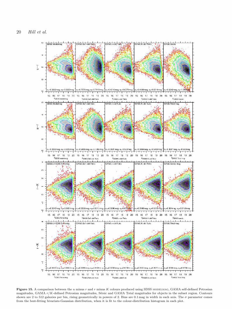
In order to identify the optimal photometric system, we as-sume that intrinsic colour distribution of a population ofgalaxies can be approximated by a double-Gaussian distri-bution (the superposition of a pair of Gaussian distributionswith different mean and standard deviation parameters).This distribution can model the bimodality of the galaxypopulation. The presence of noise will broaden the distri-bution; hence the narrowest colour distribution reveals theoptimal photometric system for calculating the colours ofgalaxies, and therefore deriving accurate SEDs. Figure 15shows the (u− r) and (r −K) colour distributions for eachphotometric system, for objects within our subset region.In order to calculate the dispersion in the colour distribu-tion, we generate colour-distribution histograms (with binsof 0.1mag), and find the double-Gaussian distribution pa-rameters that best fit each photometric system. The best-fitting standard deviation parameters for each sample areshown at the bottom of each plot, and are denoted σX,1 andσX,2 (where X is the photometric system fitted). The sam-ple with the smallest set of σ parameters should provide theoptimal photometric system.The SDSS, GAMA r-defined aperture and GAMA K-defined distributions (the first, third and fourth diagrams onthe top two rows) show a very similar pattern; a tight dis-tribution of objects with a small number of red outliers. Asexpected, when we use apertures that are defined separatelyin each filter (the second diagram on the top two rows),the colour distribution of the population is more scattered(σPetro,1 = 0.7576mag, σPetro,2 = 0.7919mag, σAuto,1 =0.5886mag, σAuto,2 = 0.7086mag) and does not show thebimodality visible in the matched aperture photometry (atthe bright end of the distribution there are two distinct sub-populations; one sub-population above u − r = 2mag, theother below). For the same reason, and probably becauseof the low quality of the observations, the (u − r) plot us-ing the Sersic magnitudes (the final diagram on the top row)has the broadest colour distribution (σSersic,1 = 0.6242mag,σSersic,2 = 1.098mag), although it is well behaved in (r-K).To generate a series of (r − K) colours using the UKIDSSsurvey (leftmost plot on the bottom two rows), we havetaken all galaxies within the UKIDSS catalogue4 and match

4 We run a query at the WSA on UKIDSSDR5PLUS looking forall objects within our subset region with lasSource.pGalaxy >

0.9 & lasSource.kPetroMag < 20 - equivalent to KAB <

21.9mag

them (with a maximum tolerance of 5 arcsec) to a copy ofthe tiling catalogue that had previously been matched withthe K band aperture-defined catalogue. The distribution of(r − K) colours taken from the SDSS and UKIDSS surveycatalogues is the first diagram on the bottom two rows ofthe image. As the apertures used to define the UKIDSS andSDSS sources are not consistent, we find that the tightest(r−K) distribution comes from the GAMA K-defined aper-ture sample (fourth from the left on the bottom row, withσAuto,1 = 0.3137 mag, σAuto,2 = 0.4921mag). The GAMAsample that relies on matching objects between self-definedobject catalogues (the second diagram on the bottom tworows) has the broadest distribution (σPetro,1 = 0.3359mag,σPetro,2 = 0.6015mag). The distribution of sources in theSersic (r − K) colour plot is much tighter than in the(u − r), though still not as tight as the distribution in thefixed aperture photometric systems (σSersic,1 = 0.364mag,σSersic,2 = 0.6159mag). Figure 15 confirms the utility ofthe GAMA method: by redoing the object extraction our-selves, we have generated self-consistent colour distribu-tions based on data taken by multiple instruments thathas a far smaller scatter than a match between the sur-vey source catalogues (σSDSS+UKIDSS,1 = 0.3342mag,σSDSS+UKIDSS,2 = 0.5807mag).We provide one more comparison between our colour dis-tribution and that provided by SDSS and UKIDSS surveydata. Figure 16 displays the X−H distribution produced bythe GAMA galaxies with complete ugrizY JHK photome-try and good quality redshifts within 0.033 < z < 0.6. Theeffective wavelengths of the filter set for each galaxy areshifted using the redshift of the galaxy. The colour distri-bution provided by the GAMA photometry produces feweroutliers than the SDSS/UKIDSS survey data sample, and iswell constrained by the Bruzual & Charlot (2003) models.

7 FINAL GAMA PHOTOMETRY

Sections 5 and 6 show that the optimal deblending out-come is produced by the original SDSS data, but the bestcolours come from our r-defined aperture photometry (Sec-tion 6.3). We see that our r-defined aperture photometryagrees with the SDSS petromag photometry. However, wehave also demonstrated that SDSS petromag misses fluxwhen compared to our Sersic total magnitude. Here we com-bine these datasets to arrive at our final photometry. Wecombine the SDSS deblending outcome with our r-definedaperture colours and the Sersic total-magnitude to produceour best photometric solution.

7.1 Sersic magnitudes

To check the reliability of the Sersic photometry pipeline,we must examine its distribution against a photometric sys-tem we consider reliable. We examine the distribution of theSersic photometry against our r-defined AUTO photometry.Figure 17 shows the distribution of Sersic - GAMA r-definedAUTO magnitude against r-defined AUTO magnitude forall objects in the GAMA sample that have passed our star-galaxy separation criteria and have credible AUTO mag-nitudes. Whilst there is generally a tight distribution, thescatter in the u band, in particular, is a cause for concern.

20 Hill et al.

Figure 15. A comparison between the u minus r and r minus K colours produced using SDSS modelmag, GAMA self-defined Petrosianmagnitudes, GAMA r/K-defined Petrosian magnitudes, Sersic and GAMA Total magnitudes for objects in the subset region. Contoursshown are 2 to 512 galaxies per bin, rising geometrically in powers of 2. Bins are 0.1mag in width in each axis. The σ parameter comesfrom the best-fitting bivariate-Gaussian distribution, when it is fit to the colour-distribution histogram in each plot.

GAMA: The photometric pipeline 21

Figure 16. A comparison between the X − H colours produced using SDSS magnitudes and GAMA Total magnitudes. Data comesfrom all GAMA galaxies with good quality redshifts (0.033 < z < 0.6) and complete ugrizY JHK photometry. Effective wavelengths arecalculated from the redshift of the galaxy and the filter effective wavelength, and the dataset is binned into a 50×50 bin matrix. TwoBruzual-Charlot 03 SSP instantaneous-burst models are also plotted. Both models use the Chabrier (2003) IMF, with mass cutoffs at0.1 and 100M⊙. Stellar evolution is undertaken using the Padova 1994 prescription. The dark grey line is a model evolved to 11Gyr ,with Z=0.05 and Y=0.352. The purple line is a model evolved to 0.25Gyr, using Z=0.02 (Z⊙) and Y=0.28.

Graham et al. (2005) analytically calculate how the ratio ofSersic flux to Petrosian flux changes with the Sersic indexof the object. The fraction of light missed by a Petrosianaperture is dependent upon the light profile of source. Fig-ure 19 shows the distribution of Sersic - GAMA r-definedPetrosian magnitude against Sersic index, redshift, absoluteand apparent magnitude for all r-band objects in the GAMAsample that have passed our star-galaxy separation criteria,and have credible r, u and K r-defined PETRO magnitudes.Graham et al. report a 0.20mag offset for an n = 4 pro-file, and a 0.50mag offset for an n = 8 profile. The medianrSersic − rPetrosian offset for objects with 3.9 < n < 4.1 inthis sample is −0.115mag, with rms scatter of 0.212mag,and −0.408mag, for objects with 7.9 < n < 8.1, with rmsscatter of 0.292mag. Both results agree with the reported

values. We have plotted the magnitude offset with Sersic in-dex function from Figure. 2 (their Panel a) of Graham et al.(2005) in the uppermost plot of Figure 19. The functionis an extremely good match to our photometry. Figure 18shows the distribution of Sersic - SDSS cmodel magnitudeagainst Sersic index, redshift, absolute and apparent magni-tude for all r-band objects in the GAMA sample that havepassed our star-galaxy separation criteria, and have credibler, u and K r-defined PETRO magnitudes. The distributionsare very similar to those produced by the Sersic-Petrosiancolours in Figure 19. An exception is the distribution withSersic index, where the Sersic - cmodel offset is distributedcloser to 0mag, until n=4, at which point the Sersic magni-tude detects more flux. As the cmodel magnitude is definedas a combination of n=1 and n=4 profiles, it is unsurpris-

22 Hill et al.

ing that it cannot model high n profile sources as well asthe GAMA Sersic magnitude, which allows the n parametergreater freedom.The r band Sersic magnitude shows no anomalous be-haviour. Sersic profiling is reliable when undertaken usingthe higher quality SDSS imaging (particularly gri), but notwhen using the noisier u band data. It is clear that theu band Sersic magnitude is not robust enough to supportdetailed scientific investigations. In order to access a Sersic-style total magnitude in the u band, we are therefore forcedto create one from existing, reliable data. We devise such anapproach in Section 7.2.

7.2 ‘Fixed aperture’ Sersic magnitudes

As mentioned in Section 4.4, the Sersic magnitude is takenfrom a different aperture in each band. We therefore cannotuse Sersic magnitudes to generate accurate colours (comparethe scatter in the Sersic colours and the AUTO colours inFigure 20). We also do not consider the u band Sersic mag-nitudes to be credible (see Section 7.1). However, we alsobelieve that the r band Sersic luminosity function may bemore desirable than the light-distribution defined aperturer band luminosity functions. The calculation of the totalluminosity density using a non-Sersic aperture system mayunderestimate the parameter. We require a system that ac-counts for the additional light found by the Sersic magni-tude, but also provides a credible set of colours.We derive a further magnitude Xtotal, using the equationXtotal = (Xauto − rauto) + rSersic, where auto is the r-defined AUTO magnitude. In effect, this creates a measurethat combines the total r band flux with optimal colours, us-ing SDSS deblending to give us the most accurate catalogueof sources (by matching to the GAMA master catalogue);the best of all possibilities. We accept that this assumes thatthe colour from the r-defined AUTO aperture would be thesame as the colour from a r-defined Sersic aperture, how-ever, this is the closest estimation to a fixed Sersic aperturewe can make at this time.

7.3 Uncertainties within the photometry

The gain value in SDSS data is constant within each stripebut varies between stripes. The SDSS mosaic creationprocess that is detailed in sections 3.2 and 3.4 combinesimages from a number of different stripes to generatethe master mosaic. As the mosaics are transformed fromdifferent zeropoints, the relationship between electronsand pixel counts will be different for each image. Thismosaic must suffer from variations in gain. The SExtractorutility can be set up to deal with this anomaly, by usingthe weightmaps generated by SWARP. However, this mayintroduce a level of surface brightness bias into the resultingcatalogue that would be difficult to quantify. We calculatethe SExtractor magnitude error via the first quartile value,taken from the distribution of gain parameters used tocreate the mosaic. The Gain used in the SDSS calculation isthe average for the strip. The SExtractor error is calculatedusing Equation 5, where A as is the area of the aperture, σis the standard deviation in noise and F is the total fluxwithin the aperture. By using the first quartile gain value,

we may be slightly overestimating the Fgain

component ofthe magnitude uncertainty calculation. However, given theamount of background noise in the mosaic, this componentwill constitute only a small fraction towards the error in thefainter galaxies, and in the brighter galaxies the uncertaintyin magnitude due to the aperture definition will be muchgreater than the SExtractor magnitude error itself. TheSExtractor magnitude error is calculated separately foreach aperture type, and is available within the GAMAphotometric catalogues.

∆m =1.0857

√

Aσ2 + Fgain

F(5)

We have attempted to quantify the uncertainty due to theaperture definition, in order to calculate its extent relative tothe SExtractor magnitude error. We use the cleaned sam-ple defined in section 6.1. The dispersion in calculated mag-nitude between our different photometric methods for thissample are shown in Figures 9, 10, 11, 12 and 13. Figure 21shows the relative scales of the uncertainty due to a galaxy’saperture definition (calculated from the standard deviationin AUTO/PETRO luminosities from the SDSS survey andour r/K/self-defined catalogues) and the error generated bySExtractor in the r band. The aperture definition uncer-tainty is generally much greater than that due to backgroundvariation and S

Nthat SExtractor derives. Figure 22 shows

how this standard deviation in a galaxy’s r band magnitudechanges with apparent magnitude. Whilst this uncertaintyis larger than the SExtractor magnitude error, it is fun-damentally a more consistent judgement of the uncertaintyin a given galaxy’s brightness as it does not assume thatany particular extended-source aperture definition is correct.Whilst the dispersion of the relationship increases with ap-parent magnitude (along with the number of galaxies), themodal standard deviation is approximately constant. Takingthis to be a good estimate of the average uncertainty in theapparent magnitude of a galaxy within our sample, we haveconfidence in our published apparent magnitudes to within±0.03mag in gri, ±0.06mag in z, and ±0.20mag in u. Wecalculate the same statistics in the NIR passbands (thoughwithout SDSS Petromag). We have confidence in our pub-lished apparent magnitudes within ±0.05mag in Y JHK;approximately two and a half times the size of the photo-metric rms error UKIDSS was designed to have (±0.02mag,Lawrence et al. 2007).

7.4 Number counts

In order to construct a unbiased dataset, it is necessary forus to calculate the apparent magnitude where the GAMAsample ceases to be complete.

7.4.1 Definition of GAMA galaxy sample used in this

section

The GAMA sample used in this section is defined as thoseSDSS objects that are within the area that has completeugrizY JHK colour coverage, and have passed the star-galaxy separation criteria. Of the 908022 objects in theGAMAmaster catalogue, only 124622 fulfil this criteria. The

GAMA: The photometric pipeline 23

Figure 17. Sersic minus GAMA r-defined Auto magnitude against r-defined Auto magnitude, in all nine bands, for all objects inthe GAMA sample that pass our star-galaxy separation criteria, and have credible ugrizY JHK r-defined Auto magnitudes. Contoursincrease geometrically in powers of 2, from 4 to 512. Bins are 0.1mag (x axis) × 0.05mag (y axis) in size.

area of sky that has complete GAMA ugrizY JHK cover-age is 129.1232 ± 0.0008 sq deg; 89.7% of the entire GAMAregion. All magnitudes in this section are r-defined AUTO

magnitudes, unless otherwise defined.

7.4.2 Determination of apparent magnitude limits

Figure 23 shows how the sky density of GAMA galaxies inthe nine passbands varies with apparent magnitude. Thedistributions peak in the 0.1 magnitude bins centred atu = 21.25, g = 20.55, r = 19.75, i = 19.25, z = 18.75,Y = 18.65, J = 18.45, H = 18.05 and K = 17.75mag. Ta-bles 7, 8 and 9 contain the number counts of GAMA galaxiesin ugrizY JHK, this time using 0.25 magnitude bins. Pois-sonian uncertainties are also included. Both sets of data havebeen converted to deg−2 mag−1 units.

The r band number count drop off, despite hitting thepetromag r= 19.8mag GAMA main sample magnitudelimit, is not absolute because the SDSS limit was extendedto petromag r= 20.5mag in the GAMA 12 region sothat useful filler objects could be selected, and becauseradio/K/z band selected objects in G9 and G15 will alsobe included within the catalogue. Objects that are fainterthan rmodel = 20.5mag (722 sources; 0.5% of the sample)will be due to differences in object extraction between SDSSand SExtractor, as mentioned in previous sections.The turnovers in Figure 23 will occur where the r = 19.8maglimit is reached for galaxies with the median passband − rcolour. We are within the domain where the number ofgalaxies within a magnitude bin increases linearly with in-creasing apparent magnitude, but a deviation from this re-lationship is visible in the figure approximately 3 magnitude

24 Hill et al.

Figure 18. Sersic r - SDSS cmodel r magnitude against Sersic index, SDSS r cmodel magnitude, z, Mr,Sersic for all objects in theGAMA sample that have passed our star-galaxy separation criteria, and have credible urK r-defined Petrosian magnitudes. Contoursincrease geometrically in powers of 2, from 4 to 512.

GAMA: The photometric pipeline 25

Figure 19. Sersic r - GAMA r-defined Petrosian r against Sersic index, r-defined r band Petrosian magnitude, z, Mr,Sersic for allobjects in the GAMA sample that have passed our star-galaxy separation criteria, and have credible urK r-defined Petrosian magnitudes.Contours increase geometrically in powers of 2, from 4 to 512. The brown function plotted in the Sersic r - GAMA r-defined Petrosianr against Sersic index plot is taken from Figure. 2 (upper panel) of Graham et al. (2005).

26 Hill et al.

−1012345 uAUTO − rAUTO

u−

r

−1

0

1

2 gAUTO − rAUTO

g−

r

−1

0

1

2 rAUTO − iAUTO

r−i

−1

0

1

2

3rAUTO − zAUTO

r−z

−1

0

1

2

3rAUTO − YAUTO

r−Y

−1

0

1

2

3 rAUTO − JAUTO

r−J

−1

0

1

2

3 rAUTO − HAUTO

r−H

−1

0

1

2

3

16 17 18 19 20

rAUTO − KAUTO

rAUTO

r−K

uSersic − rSersic

gSersic − rSersic

rSersic − iSersic

rSersic − zSersic

rSersic − YSersic

rSersic − JSersic

rSersic − HSersic

16 17 18 19 20

rSersic − KSersic

rSersic

uSDSS − rSDSS

gSDSS − rSDSS

rSDSS − iSDSS

16 17 18 19 20

rSDSS − zSDSS

rSDSS

Figure 20. X-r distributions from GAMA r-defined Auto magnitudes, GAMA Sersic magnitudes and SDSS petromags (left to right),against r, for all X = u,g,i,z,Y ,J ,H and K. Sources used are those within the subset region with credible Auto and Sersic magnitudes,and without the SDSS saturated object bit set. Contours increase geometrically in powers of 2, from 2 to 512 galaxies bin−1. Bins are0.1mag × 0.1mag in size

GAMA: The photometric pipeline 27

0.01 0.02 0.03 0.04 0.05 0.06 0.07

1

2

3

4

5

6

7

8

9

10

11

12

13

14

15

σSDSS and all AUTO+PETRO r band magnitudes (mag)

r de

fined

SE

xtra

ctor

MA

GE

RR

_AU

TO

_r (x

10−3

mag

)

Figure 21. The distribution of standard deviation in r bandapparent magnitude against SExtractor’s calculated magnitudeerror (using the first quartile gain from the gain distribution ofthe mosaic’s input images) for our clean sample of galaxies, usingSDSS, r-defined, K-defined and self-defined AUTO and PETROmagnitudes to calculate the standard deviation. Contours rise lin-early by 16 galaxies bin−1, ranging from 8 to 120 galaxies bin−1.Bins are 0.004mag (x axis) × 0.001mag (y axis) in size.

rSDSS Petro

σ SD

SS

, all

Aut

o an

d al

l Pet

ro m

agni

tude

s

17.0 17.5 18.0 18.5 19.0 19.5

0

0.01

0.02

0.03

0.04

0.05

0.06

0.07

0.08

0.09

0.1

0.11

rSDSS Petro

σ SD

SS

, r d

efin

ed A

uto

and

Pet

ro m

agni

tude

s

17.0 17.5 18.0 18.5 19.0 19.5

0

0.01

0.02

0.03

0.04

0.05

0.06

0.07

0.08

0.09

0.1

0.11

rSDSS Petro

σ SD

SS

, sel

f def

ined

Aut

o an

d P

etro

mag

nitu

des

17.0 17.5 18.0 18.5 19.0 19.5

0

0.01

0.02

0.03

0.04

0.05

0.06

0.07

0.08

0.09

0.1

0.11

rSDSS Petro

σ SD

SS

, K d

efin

ed A

uto

and

Pet

ro m

agni

tude

s

17.0 17.5 18.0 18.5 19.0 19.5

0

0.01

0.02

0.03

0.04

0.05

0.06

0.07

0.08

0.09

0.1

0.11

Figure 22. The distribution of standard deviation in r band ap-parent magnitude against apparent magnitude for our clean sam-ple of galaxies, using four different sets of magnitudes to calculatethe standard deviation in each case. Contours rise linearly by 20galaxies bin−1, ranging from 10 to 170 galaxies bin−1. Bins are0.1mag (x axis) × 0.01mag (y axis) in size.

Band Sources Redshifts % Redshifts

Star-galaxy separa-tion criteria only

124622 82926 66.5

u621.0 46006 39767 86.4g620.3 67913 58956 86.8r619.8 106032 79672 75.1i619.0 74885 66981 89.4z618.5 59470 55202 92.8Y618.4 57739 53339 92.4J618.2 60213 54264 90.1H617.8 55734 51033 91.6K617.5 46424 43252 93.2

Table 6. The number of sources within the star-galaxy separa-tion and apparent magnitude limited GAMA samples that havea complete set of good ugrizY JHK r-defined magnitudes, thenumber of those sources that have redshifts from first and secondyear data and the percentage redshift completeness. Apparentmagnitudes are r-defined magnitudes, using the AB magnitudesystem.

bins before the turnover occurs in all bands except r. Thiseffect is due to colour incompleteness becoming a factor. Un-fortunately, despite our radio/K/z selection, there will be apopulation of objects that are bright in other passbands, buttoo faint in r to be included within our sample. Assuming thepassband−r colour distribution is approximately Gaussian,this population will feature predominantly in the apparentmagnitude bins near the turnover, causing the characteristicflattening we see. Accounting for this effect, we define theapparent magnitude sample limits of our sample to be a fewbins brighter than this turnover, where the linear relation-ship still holds. Our apparent magnitude limits are set tou = 21.0, g = 20.3, r = 19.8, i = 19.0, z = 18.5, Y = 18.4,J = 18.2, H = 17.8 and K = 17.6mag.

7.4.3 GAMA apparent-magnitude limited catalogues

Table 6 contains the sizes of the apparent magnitude lim-ited samples, and their current redshift completeness. Ourmagnitude limited optical samples contain approximatelyforty thousand less galaxies than the equivalent samples inBlanton et al. (2003), which covers the SDSS DR2 region,but extend two magnitudes deeper. When we compare ournumber counts to 6dFGS (Jones et al. 2009); our samplesare also smaller in area coverage, but similar in size andmuch deeper in magnitude completeness. Hill et al. (2010),our previous attempt at defining a sample across the opticaland NIR (combining MGC, SDSS and UKIDSS data to forma B band selected ugrizY JHK catalogue), was just onetenth of the size and was 0.2−1.8mag shallower. Currently,a large fraction of our samples have not been spectroscop-ically sampled. After the completion of the 2008-2009 allo-cations of AAOmega spectroscopy, our apparent magnitudesamples have > 75% completeness. It is anticipated that thisstatistic will have raised to > 95% after the completion ofthe 2010 allocation.

7.5 Incorporating GALEX data

We have also combined the GAMA sample with UV data.The GAMA master catalogue has been matched to GALEXphotometry (Wyder et al. 2005). As GALEX observations

28 Hill et al.

1

5

10

50

100

500

1000

mr defined AUTO

N d

m (

mag

−1de

g−2)

13 14 15 16 17 18 19 20 21

u

g

r

i

z

Y

J

H

K

Figure 23. Number counts of GAMA galaxies (sources that have passed our star-galaxy separation criteria) with good ugrizY JHK

colours, split into 0.1 magnitude bins and divided by the total area they cover. Error bars shown are for Poissonian number counts.

are low resolution (typical imaging FWHM ∼ 10 arcsec), thematching is complex compared to the simple UKIDSS/SDSSmatching described within this paper as a number of sepa-rate SDSS objects may be matched to one larger GALEX ob-ject. The precise method of generating the GALEX matchesis described in Robotham et al (in prep). In summary, allSDSS objects within the 90% Petrosian radius of a GALEXsource are considered to be contributing flux to that source.The flux of the GALEX object is then apportioned to theSDSS objects, with the alloted fraction calculated via thedistance between the SDSS and GALEX object. If no othernearby source is within 2.5mag (in g) of the closest match,all flux is assigned to the closest match. GALEX has twodistinct filters NUV and FUV . The generated magnitudesare stored within columns labelled MAG AUTO FUV andMAG AUTO NUV.

7.6 SED fits using GAMA data

The SEDs of 10 galaxies selected at random from the GAMAsample are shown in Figure 24. We show the GAMA-GalexUV luminosities, GAMA Total luminosities, Petrosian lu-minosities taken from the UKIDSS and SDSS surveys, and2 Bruzual-Charlot (Bruzual & Charlot 2003) galaxy modelswith different ages and metallicities. The models are nor-malised via least squares best-fitting to the 9 GAMA data-points. For image clarity, we do not show the uncertaintieson SDSS and UKIDSS datapoints. GAMA UV uncertain-ties are taken from SExtractor magnitude errors. GAMAoptical and NIR uncertainties are calculated using the stan-dard deviation in the luminosity when different photometricmethods are used (following the method described in Section7.3). In some cases, the photometry provided by Survey-catalogues and the GAMA photometry are near identical,and match the galaxy models well (see 216774 and 137440

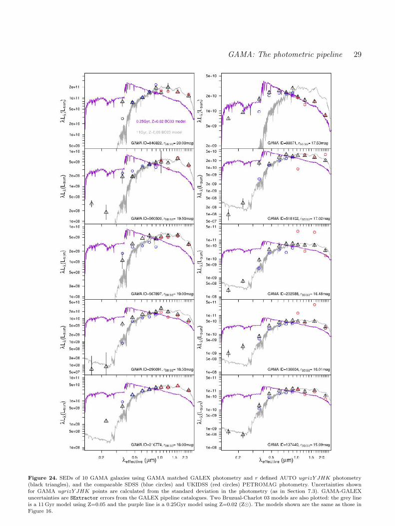
GAMA: The photometric pipeline 29

Figure 24. SEDs of 10 GAMA galaxies using GAMA matched GALEX photometry and r defined AUTO ugrizY JHK photometry(black triangles), and the comparable SDSS (blue circles) and UKIDSS (red circles) PETROMAG photometry. Uncertainties shownfor GAMA ugrizY JHK points are calculated from the standard deviation in the photometry (as in Section 7.3). GAMA-GALEXuncertainties are SExtractor errors from the GALEX pipeline catalogues. Two Bruzual-Charlot 03 models are also plotted: the grey lineis a 11Gyr model using Z=0.05 and the purple line is a 0.25Gyr model using Z=0.02 (Z⊙). The models shown are the same as those inFigure 16.

30 Hill et al.

u(mag)

Nu(m)±σNu(m)

(deg−2 (mag)−1)g(mag)

Ng(m)±σNg(m)

(deg−2 (mag)−1)

r(mag)

Nr(m)±σNr (m)

(deg−2 (mag)−1)

12.125 0.031 ± 0.015 10.125 0 ± 0 10.125 0.031 ± 0.01512.375 0 ± 0 10.375 0 ± 0 10.375 0 ± 012.625 0 ± 0 10.625 0 ± 0 10.625 0 ± 012.875 0 ± 0 10.875 0.031 ± 0.015 10.875 0.031 ± 0.01513.125 0 ± 0 11.125 0 ± 0 11.125 0 ± 013.375 0.031 ± 0.015 11.375 0 ± 0 11.375 0.124 ± 0.03113.625 0.093 ± 0.027 11.625 0.031 ± 0.015 11.625 0.062 ± 0.02213.875 0.062 ± 0.022 11.875 0 ± 0 11.875 0 ± 014.125 0.093 ± 0.027 12.125 0.062 ± 0.022 12.125 0.031 ± 0.01514.375 0.062 ± 0.022 12.375 0.124 ± 0.031 12.375 0.031 ± 0.01514.625 0.062 ± 0.022 12.625 0.031 ± 0.015 12.625 0.062 ± 0.02214.875 0.062 ± 0.022 12.875 0.031 ± 0.015 12.875 0.155 ± 0.03515.125 0.124 ± 0.031 13.125 0.031 ± 0.015 13.125 0.217 ± 0.04115.375 0.248 ± 0.044 13.375 0.062 ± 0.022 13.375 0.186 ± 0.03815.625 0.279 ± 0.046 13.625 0.062 ± 0.022 13.625 0.558 ± 0.06615.875 0.527 ± 0.064 13.875 0.248 ± 0.044 13.875 0.589 ± 0.06816.125 0.929 ± 0.085 14.125 0.248 ± 0.044 14.125 0.712 ± 0.07416.375 1.735 ± 0.116 14.375 0.712 ± 0.074 14.375 1.425 ± 0.10516.625 1.828 ± 0.119 14.625 0.62 ± 0.069 14.625 1.611 ± 0.11216.875 2.478 ± 0.139 14.875 0.836 ± 0.08 14.875 3.16 ± 0.15617.125 3.098 ± 0.155 15.125 1.27 ± 0.099 15.125 3.253 ± 0.15917.375 4.616 ± 0.189 15.375 2.478 ± 0.139 15.375 4.771 ± 0.19217.625 6.01 ± 0.216 15.625 2.447 ± 0.138 15.625 6.536 ± 0.22517.875 8.457 ± 0.256 15.875 4.089 ± 0.178 15.875 8.333 ± 0.25418.125 11.772 ± 0.302 16.125 4.213 ± 0.181 16.125 13.352 ± 0.32218.375 17.1 ± 0.364 16.375 6.32 ± 0.221 16.375 17.286 ± 0.36618.625 22.273 ± 0.415 16.625 9.139 ± 0.266 16.625 24.783 ± 0.43818.875 31.815 ± 0.496 16.875 13.166 ± 0.319 16.875 34.2 ± 0.51519.125 44.763 ± 0.589 17.125 16.728 ± 0.36 17.125 46.808 ± 0.60219.375 58.58 ± 0.674 17.375 24.225 ± 0.433 17.375 64.28 ± 0.70619.625 84.973 ± 0.811 17.625 31.722 ± 0.496 17.625 85.933 ± 0.81619.875 117.159 ± 0.953 17.875 42.719 ± 0.575 17.875 118.491 ± 0.95820.125 159.754 ± 1.112 18.125 58.673 ± 0.674 18.125 151.452 ± 1.08320.375 211.736 ± 1.281 18.375 74.502 ± 0.76 18.375 200.955 ± 1.24820.625 282.831 ± 1.48 18.625 101.299 ± 0.886 18.625 271.524 ± 1.4520.875 351.602 ± 1.65 18.875 132.122 ± 1.012 18.875 347.885 ± 1.64121.125 396.304 ± 1.752 19.125 170.256 ± 1.148 19.125 454.357 ± 1.87621.375 386.731 ± 1.731 19.375 222.175 ± 1.312 19.375 575.729 ± 2.112

19.625 282.428 ± 1.479 19.625 695.832 ± 2.32119.875 356.559 ± 1.662 19.875 540.445 ± 2.04620.125 446.148 ± 1.85920.375 505.471 ± 1.97920.625 492.894 ± 1.954

Table 7. Number counts for the ugr filters, using r-defined AUTO photometry, with Poissonian uncertainties.

on Figure 24). In other cases, where there is a discrepancybetween our derived luminosities and the Survey-catalogueparameters, the GAMA photometry is a better fit to themodels (e.g., 202588, 518102 on Figure 24). We thereforejudge our r-defined AUTO colours to be a significant im-provement.

7.7 Released GAMA photometry

The GAMA photometry described in this paper providesthe GamaPhotom catalogue. This catalogue is filtered andcombined with the other GAMA catalogues to produce thefirst GAMA data release, defined in Driver et al, 2010.

8 THE IMPACT OF THE PHOTOMETRIC

METHOD ON THE OBSERVED

LUMINOSITY DISTRIBUTION

8.1 Comparison between r band luminosity

functions

In order to illustrate the effect that photometric methodshave on statistical measurements of the galaxy population,we derive the r band luminosity function using 9 differentphotometric methods. We use all our photometric systemsand the original SDSS photometry, and derive luminosityfunctions from the same population of galaxies. This shouldprovide a consistent analysis for each method, removing allsystematic effects except for that produced by the photo-metric method.

GAMA: The photometric pipeline 31

i(mag)

Ni(m)±σNi(m)

(deg−2 (mag)−1)z(mag)

Nz(m)±σNz (m)

(deg−2 (mag)−1)Y(mag)

NY (m) ±σNY (m)

(deg−2 (mag)−1)

9.375 0 ± 0 9.375 0 ± 0 9.375 0.031 ± 0.0159.625 0 ± 0 9.625 0.031 ± 0.015 9.625 0 ± 09.875 0.031 ± 0.015 9.875 0 ± 0 9.875 0.031 ± 0.01510.125 0 ± 0 10.125 0.031 ± 0.015 10.125 0 ± 010.375 0.031 ± 0.015 10.375 0 ± 0 10.375 0 ± 010.625 0 ± 0 10.625 0.124 ± 0.031 10.625 0.124 ± 0.03110.875 0.124 ± 0.031 10.875 0.031 ± 0.015 10.875 0.031 ± 0.01511.125 0.031 ± 0.015 11.125 0.031 ± 0.015 11.125 0.031 ± 0.01511.375 0.031 ± 0.015 11.375 0 ± 0 11.375 0 ± 011.625 0 ± 0 11.625 0.031 ± 0.015 11.625 0.062 ± 0.02211.875 0.031 ± 0.015 11.875 0.031 ± 0.015 11.875 0.062 ± 0.02212.125 0.031 ± 0.015 12.125 0.093 ± 0.027 12.125 0.093 ± 0.02712.375 0.186 ± 0.038 12.375 0.217 ± 0.041 12.375 0.186 ± 0.03812.625 0.186 ± 0.038 12.625 0.248 ± 0.044 12.625 0.217 ± 0.04112.875 0.124 ± 0.031 12.875 0.31 ± 0.049 12.875 0.403 ± 0.05613.125 0.372 ± 0.054 13.125 0.558 ± 0.066 13.125 0.651 ± 0.07113.375 0.682 ± 0.073 13.375 0.62 ± 0.069 13.375 0.743 ± 0.07613.625 0.62 ± 0.069 13.625 1.022 ± 0.089 13.625 1.022 ± 0.08913.875 0.96 ± 0.086 13.875 1.611 ± 0.112 13.875 1.673 ± 0.11414.125 1.704 ± 0.115 14.125 1.983 ± 0.124 14.125 2.478 ± 0.13914.375 2.168 ± 0.13 14.375 3.501 ± 0.165 14.375 3.779 ± 0.17114.625 3.748 ± 0.17 14.625 4.554 ± 0.188 14.625 4.585 ± 0.18814.875 3.965 ± 0.175 14.875 5.545 ± 0.207 14.875 6.289 ± 0.22115.125 5.917 ± 0.214 15.125 8.116 ± 0.251 15.125 9.015 ± 0.26415.375 8.302 ± 0.254 15.375 11.555 ± 0.299 15.375 13.506 ± 0.32315.625 10.749 ± 0.289 15.625 16.697 ± 0.36 15.625 17.689 ± 0.3715.875 16.635 ± 0.359 15.875 21.994 ± 0.413 15.875 25.774 ± 0.44716.125 22.211 ± 0.415 16.125 32.031 ± 0.498 16.125 34.727 ± 0.51916.375 31.598 ± 0.495 16.375 43.4 ± 0.58 16.375 49.937 ± 0.62216.625 40.984 ± 0.563 16.625 61.43 ± 0.69 16.625 69.484 ± 0.73416.875 60.872 ± 0.687 16.875 83.703 ± 0.805 16.875 93.802 ± 0.852

17.125 82.464 ± 0.799 17.125 113.318 ± 0.937 17.125 124.873 ± 0.98317.375 111.367 ± 0.929 17.375 151.266 ± 1.082 17.375 161.83 ± 1.1217.625 142.995 ± 1.052 17.625 198.849 ± 1.241 17.625 221.277 ± 1.30917.875 193.397 ± 1.224 17.875 264.213 ± 1.43 17.875 292.124 ± 1.50418.125 253.432 ± 1.401 18.125 356.156 ± 1.661 18.125 375.424 ± 1.70518.375 336.423 ± 1.614 18.375 458.973 ± 1.885 18.375 480.285 ± 1.92918.625 438.093 ± 1.842 18.625 561.2 ± 2.085 18.625 549.831 ± 2.06418.875 549.336 ± 2.063 18.875 582.39 ± 2.12419.125 649.457 ± 2.24319.375 564.205 ± 2.09

Table 8. Number counts for the izY filters, using r-defined AUTO photometry, with Poissonian uncertainties.

8.2 Luminosity distribution and function

measurement

A number of techniques exist for measuring the galaxyluminosity distribution (see Willmer 1997), and functionsto parameterise it. We follow the methodology describedin Hill et al. (2010). This utilises the stepwise maximum-likelihood method (SWML), originally described in detailin Efstathiou et al. (1988), and the standard functionalform, the Schechter luminosity function (Schechter 1976).In Hill et al. (2010), we developed a unique flux limit foreach object based upon the spectroscopic limit and a colourlimit. As we are working only in the r band, the colour limitis now used to calculate the change in the magnitude limitbetween the studied photometric method and SDSS petro-

mag. We now set the apparent magnitude threshold for eachobject using raperture,limit = 19.4mag. An unfortunate sideeffect of the SWML method is that it requires normalisa-tion to calculate the luminosity density. We use the methodof luminosity density scaling described in sections 3.1.2 and

3.1.4 of Hill et al. (2010). This involves calculating the num-ber density of galaxies within a 1 magnitude range contain-ing the M∗mag galaxies, and using this to work out therequired scaling multiplier. We also account for the cosmicvariance within the GAMA regions. We calculate the sourcedensity of galaxies within a 5150 sq deg section of the SDSSsurvey (large enough for cosmic variance to be negligible)with dereddened −21.09 < Mr − 5log10h < −20.09 (i.e.M∗ − 5log10h ± 0.5mag, taking M∗ − 5log10h from the r-defined rAUTO photometry) and 0.023 < z < 0.1, and com-pare this with the source density calculated (using the samecatalogue) from the GAMA regions of sky. We find that theGAMA regions are 95.2% as dense as the SDSS superpop-ulation5, and therefore scale our φ∗ parameters upwards by

5 In essence, the GAMA survey is a post-stratified sampling ofthe SDSS, with the GAMA regions a stratum of the entire SDSSarea. The SDSS source density is a universal parameter of oursuperpopulation, and can be used to improve the accuracy of the

32 Hill et al.

J(mag)

NJ (m)±σNJ (m)

(deg−2 (mag)−1)H(mag)

NH(m)±σNH (m)

(deg−2 (mag)−1)K(mag)

NK(m)±σNK (m)

(deg−2 (mag)−1)

9.125 0 ± 0 9.125 0.031 ± 0.015 9.125 0 ± 09.375 0 ± 0 9.375 0 ± 0 9.375 0.031 ± 0.0159.625 0.031 ± 0.015 9.625 0.031 ± 0.015 9.625 0 ± 09.875 0.031 ± 0.015 9.875 0 ± 0 9.875 0.031 ± 0.01510.125 0 ± 0 10.125 0.093 ± 0.027 10.125 0.031 ± 0.01510.375 0.062 ± 0.022 10.375 0.062 ± 0.022 10.375 0.062 ± 0.02210.625 0.062 ± 0.022 10.625 0.031 ± 0.015 10.625 0.031 ± 0.01510.875 0.062 ± 0.022 10.875 0 ± 0 10.875 0.062 ± 0.02211.125 0 ± 0 11.125 0 ± 0 11.125 0 ± 011.375 0 ± 0 11.375 0.031 ± 0.015 11.375 0 ± 011.625 0.031 ± 0.015 11.625 0.124 ± 0.031 11.625 0.062 ± 0.02211.875 0.124 ± 0.031 11.875 0.155 ± 0.035 11.875 0.062 ± 0.02212.125 0.155 ± 0.035 12.125 0.248 ± 0.044 12.125 0.186 ± 0.03812.375 0.217 ± 0.041 12.375 0.372 ± 0.054 12.375 0.217 ± 0.04112.625 0.31 ± 0.049 12.625 0.527 ± 0.064 12.625 0.31 ± 0.04912.875 0.527 ± 0.064 12.875 0.774 ± 0.077 12.875 0.682 ± 0.07313.125 0.712 ± 0.074 13.125 0.867 ± 0.082 13.125 0.867 ± 0.08213.375 0.898 ± 0.083 13.375 1.518 ± 0.108 13.375 1.022 ± 0.08913.625 1.549 ± 0.11 13.625 2.23 ± 0.131 13.625 1.735 ± 0.11613.875 2.076 ± 0.127 13.875 3.098 ± 0.155 13.875 2.478 ± 0.13914.125 3.191 ± 0.157 14.125 4.492 ± 0.187 14.125 3.903 ± 0.17414.375 4.43 ± 0.185 14.375 6.041 ± 0.216 14.375 5.545 ± 0.20714.625 5.7 ± 0.21 14.625 7.806 ± 0.246 14.625 7.621 ± 0.24314.875 8.147 ± 0.251 14.875 12.763 ± 0.314 14.875 10.192 ± 0.28115.125 12.639 ± 0.313 15.125 17.72 ± 0.37 15.125 17.689 ± 0.3715.375 17.224 ± 0.365 15.375 24.194 ± 0.433 15.375 23.915 ± 0.4315.625 24.163 ± 0.433 15.625 35.036 ± 0.521 15.625 35.966 ± 0.52815.875 33.425 ± 0.509 15.875 49.379 ± 0.618 15.875 49.999 ± 0.62216.125 46.715 ± 0.601 16.125 70.413 ± 0.738 16.125 77.879 ± 0.77716.375 66.448 ± 0.717 16.375 94.298 ± 0.855 16.375 109.198 ± 0.9216.625 92.222 ± 0.845 16.625 133.237 ± 1.016 16.625 158.422 ± 1.108

16.875 121.434 ± 0.97 16.875 176.792 ± 1.17 16.875 218.272 ± 1.317.125 162.976 ± 1.123 17.125 245.781 ± 1.38 17.125 305.631 ± 1.53817.375 220.348 ± 1.306 17.375 319.602 ± 1.573 17.375 406.031 ± 1.77317.625 288.159 ± 1.494 17.625 420.931 ± 1.806 17.625 488.99 ± 1.94617.875 384.191 ± 1.725 17.875 504.448 ± 1.977 17.875 491.716 ± 1.95118.125 464.796 ± 1.897 18.125 515.229 ± 1.99818.375 521.394 ± 2.009

Table 9. Number counts for the JHK filters, using r-defined AUTO photometry, with Poissonian uncertainties.

a factor of 10.952

. The area incompleteness of the K band-defined sample is accounted for by calculating the normali-sation volume with Area=133.5 sq deg (the total coverage ofthe GAMA regions by K band UKIDSS data), rather thanthe Area=143.9 sq deg used for the other samples.

8.3 Sample selection

We limit our sample using our star-galaxy separation cri-teria and an apparent magnitude limit of r 6 19.4mag(imposed on the dereddened magnitude system used to cal-culate the luminosity function). We use a brighter appar-ent magnitude cut than that defined in Section 7.4 because19.4mag is the GAMA sample’s target completeness limitover all three regions. Brighter than this limit our sam-ples are 91.3% spectroscopically complete (using rAUTO).Our samples suffer greatly from spectroscopic incomplete-ness fainter than this magnitude limit. We impose a limit

total luminosity density estimation we make from the GAMAdataset.

based on the spectroscopic limit and a colour limit (i.e.19.4− (rSDSS−raperture)). To remove the necessity of mod-elling the K or E corrections for each galaxy, we also imposea redshift limit of 0.0033 < z 6 0.1. We adopt an evolutionβ = 0 (where E(z) = 2.5β log10(1 + z), setting β = 0 de-notes no evolution in this redshift range), and K(z) = 0.95z(following the r band in Hill et al. 2010). We use the SDSSEXTINCTION R parameter to deredden all our photomet-ric methods. We combine the data from the three GAMAregions, and treat them as one sample. Column 2 of Table10 contains our sample sizes.

8.4 The effects of surface brightness bias on the

presented luminosity distributions

Aperture selection can systematically bias the calculationof the luminosity distribution, particularly where a samplehas a high surface brightness constraint (see Cross & Driver2002, particularly their Figure 5, and Cameron & Driver2007). The SDSS photometric pipeline unfortunately is in-complete for µr,50 > 23mag arcsec−2 (see Section 3.4 ofBaldry et al. 2010 and references therein). It follows that

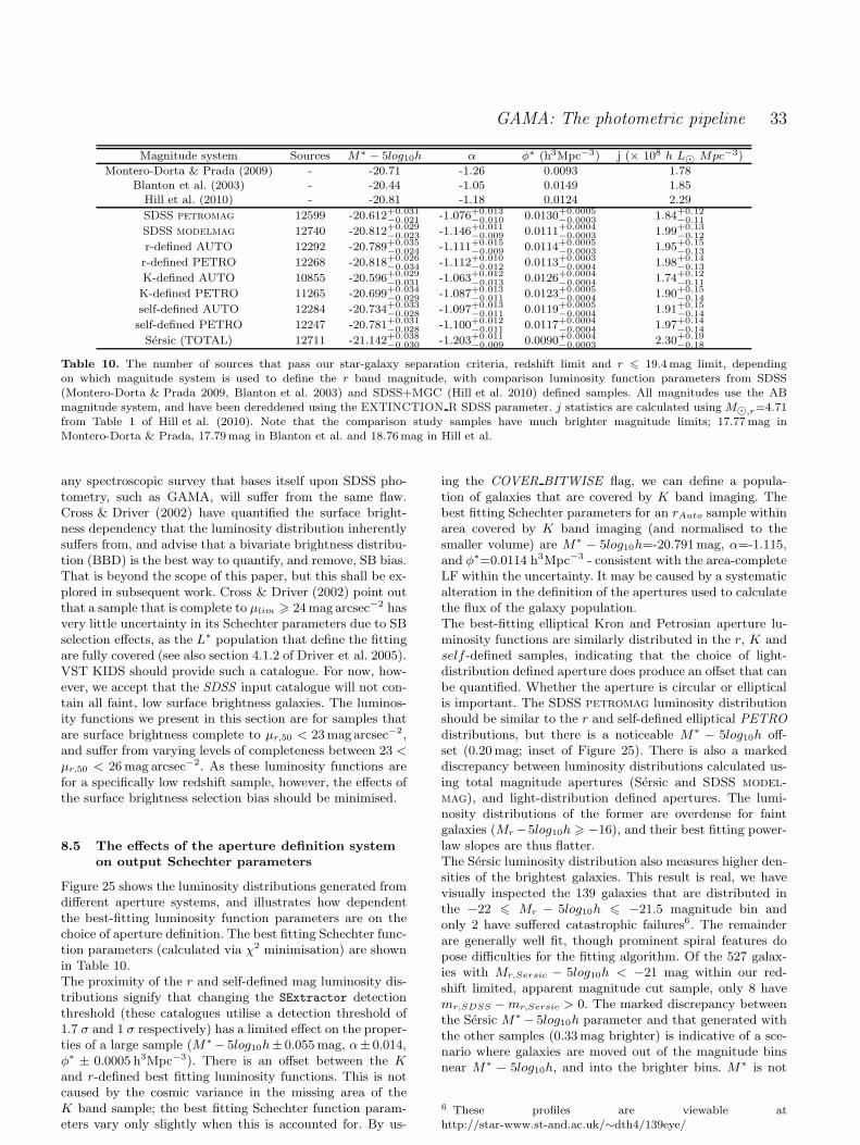
GAMA: The photometric pipeline 33

Magnitude system Sources M∗ − 5log10h α φ∗ (h3Mpc−3) j (× 108 h L⊙ Mpc−3)

Montero-Dorta & Prada (2009) - -20.71 -1.26 0.0093 1.78Blanton et al. (2003) - -20.44 -1.05 0.0149 1.85Hill et al. (2010) - -20.81 -1.18 0.0124 2.29

SDSS petromag 12599 -20.612+0.031−0.021 -1.076+0.013

−0.010 0.0130+0.0005−0.0003 1.84+0.12

−0.11

SDSS modelmag 12740 -20.812+0.029−0.023 -1.146+0.011

−0.009 0.0111+0.0004−0.0003 1.99+0.13

−0.12

r-defined AUTO 12292 -20.789+0.035−0.024 -1.111+0.015

−0.009 0.0114+0.0005−0.0003 1.95+0.15

−0.13

r-defined PETRO 12268 -20.818+0.026−0.034 -1.112+0.010

−0.012 0.0113+0.0003−0.0004 1.98+0.14

−0.13

K-defined AUTO 10855 -20.596+0.029−0.031 -1.063+0.012

−0.013 0.0126+0.0004−0.0004 1.74+0.12

−0.11

K-defined PETRO 11265 -20.699+0.034−0.029 -1.087+0.013

−0.011 0.0123+0.0005−0.0004 1.90+0.15

−0.14

self-defined AUTO 12284 -20.734+0.033−0.028 -1.097+0.013

−0.011 0.0119+0.0005−0.0004 1.91+0.15

−0.14

self-defined PETRO 12247 -20.781+0.031−0.028 -1.100+0.012

−0.011 0.0117+0.0004−0.0004 1.97+0.14

−0.14

Sersic (TOTAL) 12711 -21.142+0.038−0.030 -1.203+0.011

−0.009 0.0090+0.0004−0.0003 2.30+0.19

−0.18

Table 10. The number of sources that pass our star-galaxy separation criteria, redshift limit and r 6 19.4mag limit, dependingon which magnitude system is used to define the r band magnitude, with comparison luminosity function parameters from SDSS(Montero-Dorta & Prada 2009, Blanton et al. 2003) and SDSS+MGC (Hill et al. 2010) defined samples. All magnitudes use the ABmagnitude system, and have been dereddened using the EXTINCTION R SDSS parameter. j statistics are calculated using M⊙,r=4.71from Table 1 of Hill et al. (2010). Note that the comparison study samples have much brighter magnitude limits; 17.77mag inMontero-Dorta & Prada, 17.79mag in Blanton et al. and 18.76mag in Hill et al.

any spectroscopic survey that bases itself upon SDSS pho-tometry, such as GAMA, will suffer from the same flaw.Cross & Driver (2002) have quantified the surface bright-ness dependency that the luminosity distribution inherentlysuffers from, and advise that a bivariate brightness distribu-tion (BBD) is the best way to quantify, and remove, SB bias.That is beyond the scope of this paper, but this shall be ex-plored in subsequent work. Cross & Driver (2002) point outthat a sample that is complete to µlim > 24mag arcsec−2 hasvery little uncertainty in its Schechter parameters due to SBselection effects, as the L∗ population that define the fittingare fully covered (see also section 4.1.2 of Driver et al. 2005).VST KIDS should provide such a catalogue. For now, how-ever, we accept that the SDSS input catalogue will not con-tain all faint, low surface brightness galaxies. The luminos-ity functions we present in this section are for samples thatare surface brightness complete to µr,50 < 23mag arcsec−2,and suffer from varying levels of completeness between 23 <µr,50 < 26mag arcsec−2. As these luminosity functions arefor a specifically low redshift sample, however, the effects ofthe surface brightness selection bias should be minimised.

8.5 The effects of the aperture definition system

on output Schechter parameters

Figure 25 shows the luminosity distributions generated fromdifferent aperture systems, and illustrates how dependentthe best-fitting luminosity function parameters are on thechoice of aperture definition. The best fitting Schechter func-tion parameters (calculated via χ2 minimisation) are shownin Table 10.The proximity of the r and self-defined mag luminosity dis-tributions signify that changing the SExtractor detectionthreshold (these catalogues utilise a detection threshold of1.7 σ and 1 σ respectively) has a limited effect on the proper-ties of a large sample (M∗ − 5log10h± 0.055mag, α± 0.014,φ∗ ± 0.0005 h3Mpc−3). There is an offset between the Kand r-defined best fitting luminosity functions. This is notcaused by the cosmic variance in the missing area of theK band sample; the best fitting Schechter function param-eters vary only slightly when this is accounted for. By us-

ing the COVER BITWISE flag, we can define a popula-tion of galaxies that are covered by K band imaging. Thebest fitting Schechter parameters for an rAuto sample withinarea covered by K band imaging (and normalised to thesmaller volume) are M∗ − 5log10h=-20.791mag, α=-1.115,and φ∗=0.0114 h3Mpc−3 - consistent with the area-completeLF within the uncertainty. It may be caused by a systematicalteration in the definition of the apertures used to calculatethe flux of the galaxy population.The best-fitting elliptical Kron and Petrosian aperture lu-minosity functions are similarly distributed in the r, K andself -defined samples, indicating that the choice of light-distribution defined aperture does produce an offset that canbe quantified. Whether the aperture is circular or ellipticalis important. The SDSS petromag luminosity distributionshould be similar to the r and self-defined elliptical PETROdistributions, but there is a noticeable M∗ − 5log10h off-set (0.20mag; inset of Figure 25). There is also a markeddiscrepancy between luminosity distributions calculated us-ing total magnitude apertures (Sersic and SDSS model-

mag), and light-distribution defined apertures. The lumi-nosity distributions of the former are overdense for faintgalaxies (Mr−5log10h > −16), and their best fitting power-law slopes are thus flatter.The Sersic luminosity distribution also measures higher den-sities of the brightest galaxies. This result is real, we havevisually inspected the 139 galaxies that are distributed inthe −22 6 Mr − 5log10h 6 −21.5 magnitude bin andonly 2 have suffered catastrophic failures6. The remainderare generally well fit, though prominent spiral features dopose difficulties for the fitting algorithm. Of the 527 galax-ies with Mr,Sersic − 5log10h < −21 mag within our red-shift limited, apparent magnitude cut sample, only 8 havemr,SDSS −mr,Sersic > 0. The marked discrepancy betweenthe Sersic M∗ − 5log10h parameter and that generated withthe other samples (0.33mag brighter) is indicative of a sce-nario where galaxies are moved out of the magnitude binsnear M∗ − 5log10h, and into the brighter bins. M∗ is not

6 These profiles are viewable athttp://star-www.st-and.ac.uk/∼dth4/139eye/

34 Hill et al.

-22 -20 -18 -16 -14-5

-4

-3

-2

Figure 25. Luminosity distributions, and the best fitting Schechter functions, calculated using different aperture definitions. Inset: 1sigma chi-squared best-fit contours in the M∗-α plane. Errors on luminosity distribution points are Poissonian errors.

an independent parameter, it is correlated with the otherSchechter parameters, and accordingly the φ∗ parameter hasdeclined. The total luminosity density (j in Table 10), whilst15% higher, is consistent with that generated by the SDSSmodel magnitude within uncertainties. As our Sersic mag-nitudes are not truncated, and the SDSS model magnitudesare truncated at 7Re for a de Vaucolouers profile / 3Re foran elliptical profile, theM∗ offset between these photometricsystems is expected. We note that the residuals generated bythis Sersic-fitting process expose the requirement of multi-component galaxy decomposition; many galaxies have somestructure within their central bulges that the Sersic pipelinecannot model. A multi-component extension to this pipelineis detailed in Kelvin et al. (2010), and that paper also ex-amines any discrepancies between the Sersic and multiple-component fitting results. No matter which aperture sys-tem we use, the luminosity distribution is overdense in the

Mr − 5log10h > −16 magnitude bins when compared to thebest fitting luminosity function. This indicates an upturn inthe space density of galaxies at the dwarf-giant boundary,and the limitations of the single Schechter function fit.As noted in the introduction, the Schechter parameters gen-erated are for a sample that will suffer surface brightness in-completeness fainter than µ = 23mag arcsec−2. In a futurepaper, we intend to account for this effect by undertakinga complete bivariate brightness analysis of the sample. Thetotal luminosity densities we show here may therefore besystematically underdense due to surface brightness limita-tions (c.f. Cross & Driver 2002). It is also apparent that thesimple Schechter function parameterisation is no longer agood fit for the luminosity distribution of galaxies at faintermagnitudes; there is an obvious upturn in each sample thatis not being modelled. As the Sersic photometric system is

GAMA: The photometric pipeline 35

the only system that accounts for missing light, it is the mosteffective way of calculating the luminosity distribution.

9 SUMMARY

The GAMA photometric pipeline has been designed to com-bine photometric data from a number of sources in a scien-tific and consistent manner. We have generated a series oflarge mosaics from imaging data taken from the SDSS andUKIDSS instruments using the SWARP utility, and under-taken optical and NIR photometry on an r and K band-defined sample of sources using SExtractor. We have alsoused a Galfit based pipeline (SIGMA) to generate SersicugrizY JHK magnitudes for all sources within the GAMAsample that pass our star-galaxy separation criteria.We have created a set of r-defined source catalogues inthe ugrizY JHK passbands, calculated the apparent mag-nitude limits at which these samples are complete, and es-timated their current redshift completeness. Whilst thesesamples do not contain as many sources as those usedto calculate the SDSS luminosity functions (Blanton et al.2003, Montero-Dorta & Prada 2009), they are complete toa greater depth. Our NIR apparent magnitude limited cat-alogues are of comparable size to those produced by the6dFGS (Jones et al. 2009), with the decrease in coveragearea matched by increasing depth. Our source catalogueshave the advantage that they can be used to accurately com-pare the optical and NIR luminosity of any source withinour sample. As the aperture definition is constant we cancalculate exact colours. We have attempted to quantify thelevel of uncertainty in source flux due to the definition of theaperture. We find that the uncertainty is generally ∼ 400%of the SExtractor output uncertainty (produced by back-ground noise variations and S

N).

We have attempted to quantify the percentage of mis-matches between our catalogues and the SDSS catalogues.We have taken a subset region of our images and testedtheir results against the SDSS detection software. We havedetailed reasons for mismatches between these catalogues.They are generally an issue of different deblending decisions,artifacts, background noise or proximity to saturated stars.We find that there do seem to be some low surface bright-ness, compact objects that are missed by the SDSS detectionsoftware that are found by SExtractor, and some false SDSSdetections. These faulty sources would be removed from thespectroscopic observing list by the extensive visual classifi-cation process undertaken by the GAMA team.As our Sersic magnitudes are generated from the images thatthe profile is calculated on, the colours produced from theSersic magnitudes are liable to be inaccurate and suffer frombias due to the aperture definition. We have defined a set of’Fixed aperture’ Sersic magnitudes using the Sersic r bandmagnitude and colours from the r-defined AUTO catalogue.We recommend the use of these magnitudes, called Xtotal.These magnitudes will provide both an accurate estimate ofthe luminosity of each galaxy, and optimal colours.The GAMA photometric pipeline catalogue does not havethe breadth of focus that the existing products from theSDSS and UKIDSS surveys have. As both the instrumentgain (in SDSS only) and seeing change from frame to frame,our mosaics have variations within them that would cause

errors in the calculation of stellar photometry. We have notattempted to deal with saturated objects, which causes un-certainty at the bright end of our catalogue, or masking ofartifacts. These problems primarily affect stars, or are re-moved following the extensive visual classification programwe have undertaken. For the task our catalogues were devel-oped for, the accurate calculation of extended source aper-tures across instruments for a specific sample of extendedsources, they are more adept than the existing tools.Finally, we have generated r band luminosity distributionsand best-fitting luminosity functions from our populationof galaxies using 9 different aperture definitions: SDSS cir-cular Petrosian and Model magnitudes, r-defined ellipticalPetrosian and Auto magnitudes, K-defined elliptical Pet-rosian and Auto magnitudes, self -defined elliptical Pet-rosian and Auto magnitudes, and an elliptical Sersic totalmagnitude. We find that the r and self -defined elliptical,light-distribution defined apertures produce similar results,indicating that the choice of detection threshold is unimpor-tant. We find that there is a similar AUTO-PETRO offsetin the r, self and K-defined samples. We find that the useof circular apertures does have an effect on the best-fittingSchechter fit, with the SDSS petromag having a fainterM∗ parameter than the SExtractor samples. We also findthat the use of total magnitude systems affects the slopeof the luminosity function, with both the Sersic and SDSSmodelmag luminosity functions having a steeper α parame-ter. When we calculate the total luminosity density for eachsample we find that using the Sersic magnitude system givesus a higher value, approximately 15% higher than samplesthat use other aperture definition systems. Following visualclassification of a subsection of our sample, it is clear thatthis is not due to errors within our Sersic magnitude calcu-lation. We also note that the Schechter luminosity functiondoes not provide a good fit at the faint end of the luminositydistribution, and a clear upturn at the dwarf-giant boundaryis seen.

10 ACKNOWLEDGEMENTS

DTH and LSK are funded by STFC studentships. ASGRis funded by a STFC grant. AMH acknowledges supportprovided by the Australian Research Council through aQEII Fellowship (DP0557850).

Funding for the SDSS and SDSS-II has been providedby the Alfred P. Sloan Foundation, the ParticipatingInstitutions, the National Science Foundation, the U.S.Department of Energy, the National Aeronautics and SpaceAdministration, the Japanese Monbukagakusho, the MaxPlanck Society, and the Higher Education Funding Councilfor England. The SDSS Web Site is http://www.sdss.org/.The SDSS is managed by the Astrophysical ResearchConsortium for the Participating Institutions. The Partici-pating Institutions are the American Museum of NaturalHistory, Astrophysical Institute Potsdam, University ofBasel, University of Cambridge, Case Western ReserveUniversity, University of Chicago, Drexel University,Fermilab, the Institute for Advanced Study, the JapanParticipation Group, Johns Hopkins University, the JointInstitute for Nuclear Astrophysics, the Kavli Institute for

36 Hill et al.

Particle Astrophysics and Cosmology, the Korean ScientistGroup, the Chinese Academy of Sciences (LAMOST), LosAlamos National Laboratory, the Max-Planck-Institutefor Astronomy (MPIA), the Max-Planck-Institute forAstrophysics (MPA), New Mexico State University, OhioState University, University of Pittsburgh, University ofPortsmouth, Princeton University, the United States NavalObservatory, and the University of Washington.

The UKIDSS project is defined in Lawrence et al. 2007.UKIDSS uses the UKIRT Wide Field Camera (WFCAM;Casali et al. 2007) and a photometric system described inHewett et al. 2006. The pipeline processing and sciencearchive are described in Irwin et al (2010, in preparation)and Hambly et al. 2008.

STILTS is a set of command-line based cataloguematching tools, based upon the STIL library. It is currentlybeing supported by its author (Mark Taylor), and can bedownloaded from http://www.star.bris.ac.uk/∼mbt/stilts/.

We thank Robert Lupton for his useful comments andsuggestions when refereeing this paper.

REFERENCES

Abazajian K., et al., 2004, AJ, 128, 502Adelman-McCarthy J. K., et al., 2008, ApJS, 175, 297Andreon S., 2002, A&A, 382, 495Baldry I. K., Robotham A. S. G., Hill D. T., et al., 2010,MNRAS, 404, 86

Bertin E., Arnouts S., 1996, A&AS, 117, 393Bertin E., Mellier Y., Radovich M., Missonnier G., Dide-lon P., Morin B., 2002, in D. A. Bohlender, D. Durand,& T. H. Handley ed., Astronomical Data Analysis Soft-ware and Systems XI Vol. 281 of Astronomical Society ofthe Pacific Conference Series, The TERAPIX Pipeline. pp228–+

Blanton M. R., Hogg D. W., et al., 2003, ApJ, 592, 819Brown R. J. N., Forbes D. A., Silva D., Helsdon S. F.,Ponman T. J., Hau G. K. T., Brodie J. P., Goudfrooij P.,Bothun G., 2003, MNRAS, 341, 747

Bruzual G., Charlot S., 2003, MNRAS, 344, 1000Cameron E., Driver S. P., 2007, MNRAS, 377, 523Caon N., Capaccioli M., Rampazzo R., 1990, A&AS, 86,429

Casali M., et al., 2007, A&A, 467, 777Chabrier G., 2003, PASP, 115, 763Cohen M., Wheaton W. A., Megeath S. T., 2003, AJ, 126,1090

Cross N., Driver S. P., 2002, MNRAS, 329, 579de Vaucouleurs G., 1948, Annales d’Astrophysique, 11, 247Driver S. P., Liske J., Cross N. J. G., De Propris R., AllenP. D., 2005, MNRAS, 360, 81

Driver S. P., Norberg P., Baldry I. K., Bamford S. P., Hop-kins A. M., Liske J., Loveday J., Peacock J. A., et al.,2009, Astronomy and Geophysics, 50, 050000

Eales S., Dunne L., et al., 2009, ArXiv e-printsEfstathiou G., Ellis R. S., Peterson B. A., 1988, MNRAS,232, 431

Freeman K. C., 1970, ApJ, 160, 811

Graham A. W., 2001, AJ, 121, 820

Graham A. W., Driver S. P., 2005, Publications of the As-tronomical Society of Australia, 22, 118

Graham A. W., Driver S. P., Petrosian V., Conselice C. J.,Bershady M. A., Crawford S. M., Goto T., 2005, AJ, 130,1535

Hambly N. C., et al., 2008, MNRAS, 384, 637

Hewett P. C., Warren S. J., Leggett S. K., Hodgkin S. T.,2006, MNRAS, 367, 454

Hill D. T., Driver S. P., Cameron E., Cross N., Liske J.,Robotham A., 2010, MNRAS, pp 295–+

Høg E., Fabricius C., Makarov V. V., et al., 2000, A&A,355, L27

Ivezic Z., Lupton R. H., Schlegel D., et al., 2004, As-tronomische Nachrichten, 325, 583

Jones D. H., Read M. A., Saunders W., Colless M., JarrettT., Parker Q. A., Fairall A. P., Mauch T., Sadler E. M.,Watson F. G., et al., 2009, MNRAS, 399, 683

Kelvin L. S., Driver S. P., Robotham A. S. G., 2010, MN-RAS

Kron R. G., 1980, ApJS, 43, 305

Lawrence A., Warren S. J., et al., 2007, MNRAS, 379, 1599

Montero-Dorta A. D., Prada F., 2009, MNRAS, 399, 1106

Patterson F. S., 1940, Harvard College Observatory Bul-letin, 914, 9

Peng C. Y., Ho L. C., Impey C. D., Rix H. W., 2007, inBulletin of the American Astronomical Society Vol. 38 ofBulletin of the American Astronomical Society, DetailedDecomposition of Galaxy Images II: Fitting Spiral Arms,Bars, and Non-axisymmetric Structures in GALFIT 3.0.pp 804–+

Petrosian V., 1976, ApJ, 209, L1

Pier J. R., Munn J. A., et al., 2003, AJ, 125, 1559

Robotham A., Driver S. P., Norberg P., et al., 2010, Pub-lications of the Astronomical Society of Australia, 27, 76

Schechter P., 1976, ApJ, 203, 297

Sersic J. L., 1963, Boletin de la Asociacion Argentina deAstronomia La Plata Argentina, 6, 41

Smith A. J., Loveday J., Cross N. J. G., 2009, MNRAS,397, 868

Stoughton C., Lupton R. H., et al., 2002, AJ, 123, 485

Strauss M. A., Weinberg D. H., Lupton R. H., NarayananV. K., et al., 2002, AJ, 124, 1810

Taylor M. B., 2006, in Gabriel C., Arviset C., Ponz D.,Enrique S., eds, Astronomical Data Analysis Softwareand Systems XV Vol. 351 of Astronomical Society ofthe Pacific Conference Series, STILTS - A Package forCommand-Line Processing of Tabular Data. pp 666–+

Warren S. J., Hambly N. C., Dye S., et al., 2007, MNRAS,375, 213

Willmer C. N. A., 1997, AJ, 114, 898

Wyder T. K., Treyer M. A., Milliard B., Schiminovich D.,Arnouts S., et al., 2005, APJL, 619, L15

York D. G., et al., 2000, AJ, 120, 1579

Zacharias N., Urban S. E., Zacharias M. I., et al., 2000, AJ,120, 2131

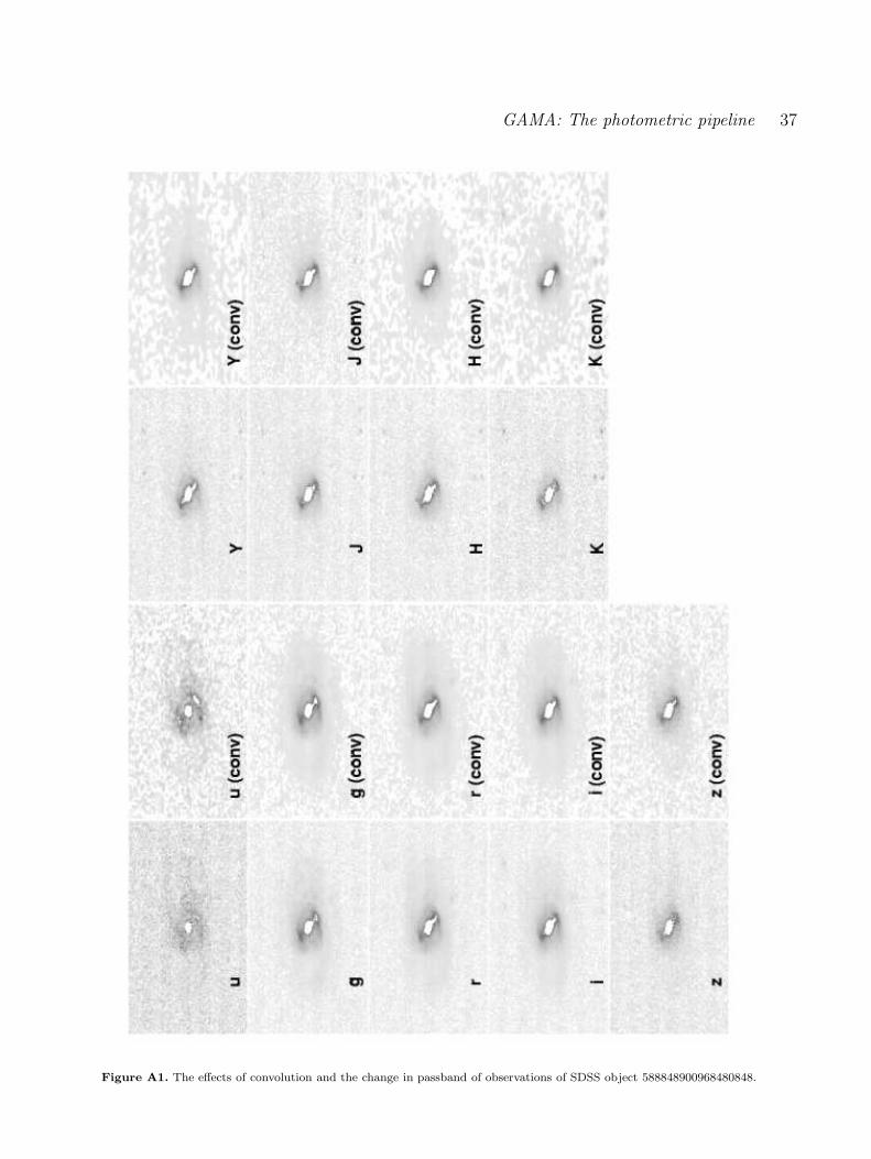
GAMA: The photometric pipeline 37

Figure A1. The effects of convolution and the change in passband of observations of SDSS object 588848900968480848.

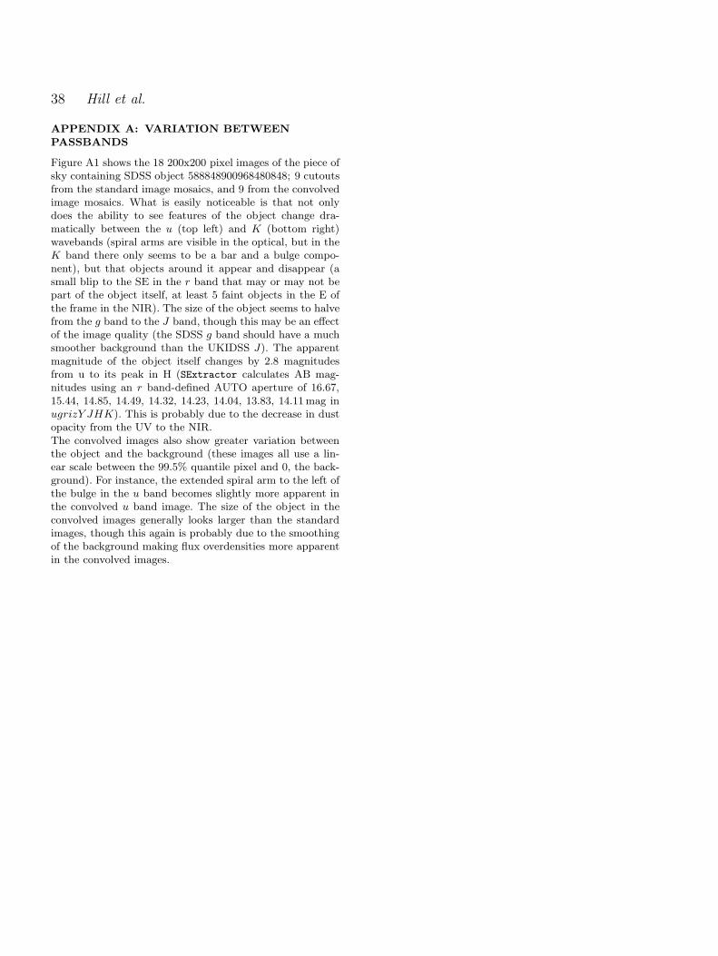
38 Hill et al.

APPENDIX A: VARIATION BETWEEN

PASSBANDS

Figure A1 shows the 18 200x200 pixel images of the piece ofsky containing SDSS object 588848900968480848; 9 cutoutsfrom the standard image mosaics, and 9 from the convolvedimage mosaics. What is easily noticeable is that not onlydoes the ability to see features of the object change dra-matically between the u (top left) and K (bottom right)wavebands (spiral arms are visible in the optical, but in theK band there only seems to be a bar and a bulge compo-nent), but that objects around it appear and disappear (asmall blip to the SE in the r band that may or may not bepart of the object itself, at least 5 faint objects in the E ofthe frame in the NIR). The size of the object seems to halvefrom the g band to the J band, though this may be an effectof the image quality (the SDSS g band should have a muchsmoother background than the UKIDSS J). The apparentmagnitude of the object itself changes by 2.8 magnitudesfrom u to its peak in H (SExtractor calculates AB mag-nitudes using an r band-defined AUTO aperture of 16.67,15.44, 14.85, 14.49, 14.32, 14.23, 14.04, 13.83, 14.11mag inugrizY JHK). This is probably due to the decrease in dustopacity from the UV to the NIR.The convolved images also show greater variation betweenthe object and the background (these images all use a lin-ear scale between the 99.5% quantile pixel and 0, the back-ground). For instance, the extended spiral arm to the left ofthe bulge in the u band becomes slightly more apparent inthe convolved u band image. The size of the object in theconvolved images generally looks larger than the standardimages, though this again is probably due to the smoothingof the background making flux overdensities more apparentin the convolved images.